Realization of an atomic quantum Hall system in four dimensions

Topological states of matter lie at the heart of our modern understanding of condensed matter systems. In two-dimensional (2D) quantum Hall insulators, the non-trivial topology, defined by the first Chern number, manifests as a quantized Hall conductance [1, 2] and protected ballistic edge modes [3]. Besides topological insulators [4] and Weyl semi-metals [5, 6] experimentally realized in 3D materials, a large variety of topological systems, theoretically predicted in dimensions $D>3$, remains unexplored [7] – among them a generalization of the quantum Hall effect in 4D [8, 9]. So far, topological properties linked with the 4D Hall effect have been revealed via geometrical charge pump experiments in 2D systems [10, 11]. A truly 4D Hall system has also been realized using electronic circuits – however, no direct evidence of topological quantization has been reported [12]. Here, we engineer an atomic quantum Hall system evolving in 4D, by coupling with light fields two spatial dimensions and two synthetic ones encoded in the electronic spin $J=8$ of dysprosium atoms [13, 14, 15]. We measure the characteristic properties of a 4D quantum Hall system, namely the quantization of its electromagnetic non-linear response by a second Chern number, and the special nature of its 3D hyperedge modes, which combine ballistic motion along one orientation and insulating behaviour in the two remaining directions. We also probe low-lying excitations, revealing non-planar cyclotron orbits in contrast with their circular equivalents in $D\leq 3$. Our findings pave the way to the exploration of interacting quantum Hall systems in 4D, from the investigation of strongly-correlated liquids [9, 16] to the simulation of high-energy models in link with quantum gravity [9] and Yang-Mills field theory [17, 18].

Dimensionality plays a prominent role in the classification of topological physical systems [7]. While different topological classes have been explored in condensed matter systems [19] – effectively described in one, two or three dimensions – higher dimensional systems can potentially be accessed with engineered materials, based on the concept of synthetic dimensions [13, 20]. In particular, different protocols have been proposed to realize a generalization of a quantum Hall insulator to 4D [21, 22, 23], both for time-reversal invariant systems (classes AI and AII, as realized with electronic circuits [12]) and in the absence of discrete symmetry (class A). In 4D, a non-trivial topology leads to specific behaviour, such as the quantization of the non-linear response to both electric and magnetic perturbations, characterized by the second Chern number $\mathcal{C}_{2}$ [9, 24, 22] – a topological invariant also relevant for tensor monopoles in high dimensions [25, 26, 27, 28]. The topology of a 4D quantum Hall insulator (class A) also gives rise to anisotropic motion at the edge of the system, ballistic along a given orientation, and still prohibited along the two remaining directions of the 3D hyperedge [29].

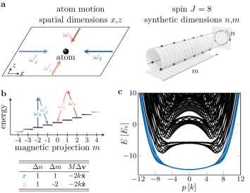
Figure 1: Scheme of the 4D atomic system. a. The atomic motion in the $xz$ plane is coupled to the internal spin $J=8$ using two-photon optical transitions along $x$ and $z$ (blue and red arrows, respectively). The spin encodes two synthetic dimensions given by the magnetic projection $m$ and its remainder $n=m\ (\mathrm{mod}\ 3)$ of its Euclidian division by 3, leading to a synthetic space of cylindrical geometry [30]. b. Scheme of the light-induced spin transitions, of first- and second-order along $x$ and $z$, respectively. They induce correlated spin-orbit dynamics, with distinct hopping along $n$ and $m$ according to the rules given in the table. c. Dispersion relation plotted as a function of the momentum $p$, for 6 values of the quasi-momentum $q$ uniformly spanning the Brillouin zone. The ground band is pictured as blue lines.

In this article, we realize an effectively 4D quantum Hall system using an ultracold sample of dysprosium atoms, whose motion along two spatial dimensions $x$ and $z$ is coupled to two synthetic dimensions encoded in the electronic spin $J=8$ (Fig. 1a). The spin-orbit coupling is generated by two-photon optical transitions [31] (Fig. 1b), such that it produces an effective magnetic field leading to the band structure of a class A Hall insulator in 4D. We reveal the quantization of the non-linear response to both electric and magnetic perturbations, except on the system edges where we observe anisotropic dispersion. We also probe cyclotron excitations of the center of mass, whose non-planar trajectories contrast with cyclotron motion in dimensions $D\leq 3$.

The coupling between motion and spin degrees of freedom is generated by a pair of lasers counter-propagating along $x$ (resp. $z$) and resonantly driving spin transitions $m\rightarrow m+1$ (resp. $m\rightarrow m-2$), while imparting a momentum kick $-2k\hat{\textbf{x}}$ (resp. $-2k\hat{\textbf{z}}$). Here, $m$ is the spin projection along $z$ ($-J\leq m\leq J$, $m$ integer), $k=2\pi/\lambda$ is the light momentum for a wavelength $\lambda=$626.1\text{\,}\mathrm{nm}$$, and we assume a unit reduced Planck constant $\hbar=1$. The atom dynamics is described by the Hamiltonian

$$H =\frac{Mv^{2}}{2}-\bigg{(}t_{x}\text{e}^{\text{i}\phi_{x}}\frac{J_{+}}{J}+t_{z}\text{e}^{\text{i}\phi_{z}}\frac{J_{-}^{2}}{J^{2}}+\text{hc}\bigg{)}+\beta\frac{J_{z}^{2}}{J^{2}},$$ (1)

where v is the atom velocity and $\phi_{\alpha}=-2k\alpha$ is the relative phase of the two laser beams involved in each Raman process $\alpha=x,z$. The laser intensities and polarisations control the amplitudes $t_{\alpha}$ and the quadratic Zeeman shift $\beta=-2t_{z}$ (see Methods).

The laser-induced spin transitions can be interpreted as hopping processes in a two-dimensional synthetic space $(m,n)$ involving the spin projection $m$ and the remainder $n=m\ (\mathrm{mod}\ 3)$ of its Euclidian division by 3 (with $n=0,1,2$) [30]. While the first-order spin coupling $J_{+}$ acts on these two dimensions in a similar manner (hopping $\Delta n^{(x)}=\Delta m^{(x)}=1$), the second-order coupling $J_{-}^{2}$ induces hoppings $\Delta n^{(z)}=1$ and $\Delta m^{(z)}=-2$ leading to differential dynamics along $m$ and $n$. The complex phases $\phi_{\alpha}$ (with $\alpha=x,z$) can be interpreted as Peierls phases upon the hopping of a charged particle on a lattice subjected to a magnetic field. Assuming unit charge, we write $\phi_{\alpha}=\int A_{\beta}\text{d}r^{\beta}=A_{n}\Delta n^{(\alpha)}+A_{m}\Delta m^{(\alpha)}$, leading to the explicit expression for the vector potential

$$\textbf{A}=\frac{1}{3}(0,0,2\phi_{x}+\phi_{z},\phi_{x}-\phi_{z})_{x,z,n,m}.$$ (2)

The magnetic field is then defined by the anti-symmetric tensor $B_{\alpha\beta}=\partial_{\alpha}A_{\beta}-\partial_{\beta}A_{\alpha}$, as

$$\textbf{B}=\frac{2k}{3}\begin{pmatrix}0&0&-2&-1\\ 0&0&-1&1\\ 2&1&0&0\\ 1&-1&0&0\end{pmatrix}.$$ (3)

Similarly to the 2D quantum Hall effect, this magnetic field gives rise to an energy separation between quasi-flat magnetic Bloch bands. Within each band, motion becomes effectively two-dimensional, with the guiding center coordinate along $n$ canonically conjugated to the position along $\hat{\bm{\nu}}=(2\hat{\textbf{x}}+\hat{\textbf{z}})/\sqrt{5}$, while $m$ is conjugated to the projection on $\hat{\bm{\mu}}=(\hat{\textbf{x}}-\hat{\textbf{z}})/\sqrt{2}$. The energy levels are indexed by the canonical momentum $\textbf{p}=M\textbf{v}+2km\hat{\textbf{x}}\ (\mathrm{mod}\ \textbf{K})$, which is conserved in the absence of external force. Here, the reciprocal lattice vector $\textbf{K}=2k(2\hat{\textbf{x}}+\hat{\textbf{z}})\parallel\hat{\bm{\nu}}$ corresponds to the momentum kick imparted on a non-trivial cycle $m\overset{z}{\rightarrow}m+2\overset{x}{\rightarrow}m+1\overset{x}{\rightarrow}m$ involving one transition along $z$ and two along $x$. In the following, we decompose the momentum as $\textbf{p}=p\hat{\bm{\xi}}+q\hat{\bm{\nu}}$, with $\hat{\bm{\xi}}=(\hat{\textbf{x}}-2\hat{\textbf{z}})/\sqrt{5}\perp\hat{\bm{\nu}}$, such that the first Brillouin zone is defined for $|q|<K/2$ and arbitrary $p$. The energy levels of the Hamiltonian (1) organize in Bloch bands shown in Fig. 1d. We focus here on the ground band, which is quasi-flat in the bulk mode region $|p|\lesssim 7k$ (see Methods).

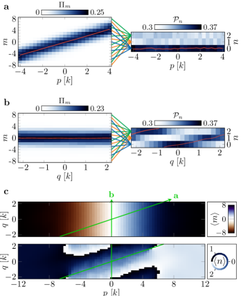
Figure 2: Hall drift along the synthetic dimensions. a. Evolution of the measured spin projections $\Pi_{m}$ and $\mathcal{P}_{n}$ as a function of $p$ upon adiabatic driving along $\hat{\bm{\mu}}$ – the spatial direction conjugated with $m$. The mean values $\langle m\rangle$ and $\langle n\rangle$ (computed as $\tfrac{3}{2\pi}\arg\langle\text{e}^{\text{i}2\pi m/3}\rangle)$ are shown as red lines. b. Same quantities plotted for a driving along $\hat{\bm{\nu}}$ – the spatial direction conjugated with $n$. c. Measurements of the mean values $\langle m\rangle$ and $\langle n\rangle$ in the Brillouin zone. The green arrows represent the driving directions considered in a and b.

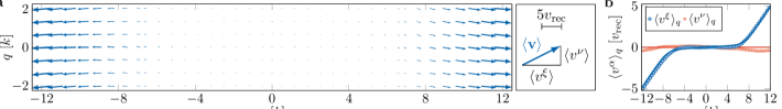
Figure 3: Frustration of motion in the bulk and anisotropic ballistic edge modes. a. Evolution of the mean velocity $\langle\textbf{v}\rangle$ versus momentum. The arrow is scaled according the mean velocity modulus. b. Measurements of the $q$-average velocity components versus $p$. The solid lines are the expected variations for the ground band of the Hamiltonian (1).

Our experiments use ultracold dilute samples of $\simeq 3.0(3)\times 10^{4}$ atoms of ¹⁶²Dy, prepared in an optical dipole trap at a temperature $T=$260(10)\text{\,}\mathrm{nK}$$. The atoms are subjected to a magnetic field $B=$221(1)\text{\,}\mathrm{m}\mathrm{G}$$ along $z$, and initially spin-polarized in the magnetic sub-level $m=-J$. We adiabatically ramp up the laser intensities to generate the spin couplings described in (1) with $t_{x}=5.69(6)\,E_{\text{rec}}$ and $t_{z}=5.1(1)\,E_{\text{rec}}$, where $E_{\text{rec}}=k^{2}/(2M)$ is the recoil energy. Starting in the $m=-J$ edge mode region with $p<7k$, we prepare arbitrary momentum states of the ground energy band by applying a weak force on a typical $1\text{\,}\mathrm{ms}$ timescale (see Methods). At the end of the experiments, we probe the velocity distribution by imaging the atomic sample after free expansion in the presence of a magnetic field gradient, such that the different $m$ states are spatially separated.

We first investigate the anomalous Hall drift in spin space upon the application of a weak force in the $xz$ plane. For a force oriented along $\hat{\bm{\mu}}$ (spatial direction conjugated to $m$), the spin projection probabilities $\Pi_{m}$ reveal a drift of the mean spin projection $\langle m\rangle$, while the mean remainder $\langle n\rangle$ remain approximately constant (Fig. 2a). An opposite behavior is observed when applying a force along $\hat{\bm{\nu}}$ (direction conjugated to $n$), with a quasi-linear variation of $\langle n\rangle$ while $\langle m\rangle$ remains constant (Fig. 2b). More generally, in the bulk of the system, where the band dispersion can be neglected, the variation with momentum of the mean values $\langle n\rangle$ and $\langle m\rangle$ can be expressed as an anomalous Hall drift governed by the antisymmetric Berry curvature tensor $\bm{\Omega}_{\text{bulk}}$, as

$$\text{d}\langle r^{\alpha}\rangle =\Omega_{\text{bulk}}^{\alpha\beta}\text{d}p_{\beta},$$ (4)

$$\bm{\Omega}_{\text{bulk}} =\textbf{B}^{-1}=\frac{1}{2k}\begin{pmatrix}0&0&1&1\\ 0&0&1&-2\\ -1&-1&0&0\\ -1&2&0&0\end{pmatrix},$$ (5)

where r is the position vector and dp is the momentum variation due to the external force. We confront this prediction to our measurements of the mean positions $\langle m\rangle$ and $\langle n\rangle$ as a function of p (Fig. 2c). In the center of the Brillouin zone $|p|\leq 4k$ (bulk mode region), we fit the measured Hall drift with the linear function (4), yielding $\{\Omega^{nx},\Omega^{nz},\Omega^{mx},\Omega^{mz}\}=\{-1.00(2),-0.98(2),-0.98(2),1.96(2)\}/(2k)$, consistent with (5). We do not measure any significant spatial drift upon the application of a force in the $xz$ plane, consistent with $\Omega^{xz}=0$. Similarly, no Hall current along $n$ is measured when applying a force along $m$ (corresponding to a perturbative Zeeman field), compatible with $\Omega^{nm}=0$ (see Methods).

Further insight on the ground band properties is provided by the mean velocity $\langle\textbf{v}\rangle$ (Fig. 3), which reveals distinct behaviours between bulk and the edge modes.

In the bulk $|p|\lesssim 7k$, the mean velocity remains much smaller than the recoil velocity $v_{\text{rec}}=k/M$ (Fig. 3b). Since $\langle\textbf{v}\rangle=\nabla_{\textbf{p}}E_{0}$, it confirms that the ground band energy $E_{0}$ is quasi-flat in the bulk (Fig. 1d). This measurement illustrates the frustration of motion induced by the magnetic field, similarly to flat Landau levels in 2D electron gases.

For $p\gtrsim 7k$, the atoms mostly occupy the edge $\textbf{r}^{\text{edge}}=J\hat{\textbf{m}}$ of the synthetic dimension $m$. We measure a non-zero mean velocity, whose $\xi$ component increases with $p$, while the $\nu$ projection remains small (Fig. 3b). This observation is characteristic of an anisotropic edge mode of a 4D quantum Hall system, which corresponds to a collection of 1D conduction channels oriented along the direction $\textbf{w}_{\text{motion}}$, with $w_{\text{motion}}^{\alpha}\propto\Omega_{\text{bulk}}^{\alpha\beta}r_{\beta}^{\text{edge}},$ here corresponding to the direction $\hat{\bm{\xi}}$ [29]. Within the edge, the motion in the plane orthogonal to $\textbf{w}_{\text{motion}}$ remains inhibited, in agreement with the measured $\nu$ velocity. A similar behaviour is found on the edge $-J\hat{\textbf{m}}$, albeit with opposite orientation of velocity.

A hallmark of 4D quantum Hall physics is the peculiar nature of excitations above the ground band, which can be linked to classical cyclotron trajectories. While cyclotron motion in 2D and 3D always corresponds to planar circular orbits, we expect more complex trajectories in 4D, involving two planar rotations occurring at different rates. In our system, each of these two elementary excitations is generated by the Raman coupling along $x$ or $z$, of corresponding frequencies $\omega_{x}$ and $\omega_{z}$ independently set by the amplitudes $t_{x}$ and $t_{z}$. We excite the atoms by applying a diabatic velocity kick, and measure the subsequent time evolution of the center of mass. We show in Fig. 4a the orbit measured for $\omega_{z}/\omega_{x}\simeq 2$, revealing a non-planar trajectory. For this integer frequency ratio, the orbit is almost closed, and is reminiscent of a Lissajous orbit (Fig. 4b). We also studied the case of degenerate frequencies $\omega_{z}\simeq\omega_{x}$, which correspond to the coupling amplitudes used for our study of the ground band. In this ‘isoclinic’ case, we recover a planar cyclotron motion akin to lower-dimensional cyclotron orbits (Fig. 4c,d).

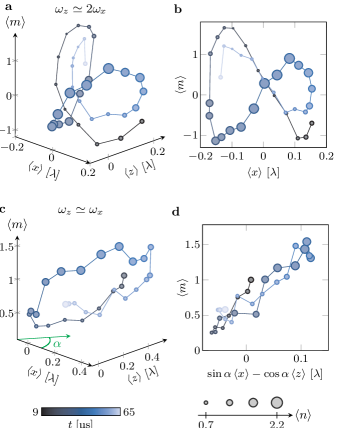
Figure 4: Cyclotron dynamics. a. Evolution of the center-of-mass position following a velocity kick, for $\omega_{z}\simeq 2\omega_{x}$. The cartesian coordinates correspond to $(x,z,m)$, while $n$ is given by the mark size. The mark color indicates the evolution time subsequent to the kick. b. Projection in the $xm$ plane corresponding to a quasi-closed Lissajouss curve. c. Cyclotron orbit measured for $\omega_{z}\simeq\omega_{x}$. The green arrow shows the viewpoint for the planar projection shown in d. d. Two-dimensional projection revealing the planar nature of the orbit viewed from the side.

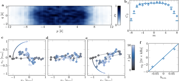
Figure 5: Topological structure of the ground band. a. Second Chern character $\rho_{2}$ computed from the product of measured Berry curvatures. b. Local second Chern marker inferred from a. c, d, e. Velocity dynamics in the $xz$ plane for three different values of the magnetic perturbation $b_{nm}=-0.066,0,0.066$, respectively. f. Precession rate $\omega_{\text{p}}$ as a function of the $b_{nm}$ field. The solid line is the prediction of (6) for the bulk second Chern character $\rho_{2}^{\text{bulk}}=3/(4k^{2})$.

The non-trivial topology of a quantum Hall system manifests in the quantization of its electromagnetic response. While involving the linear Hall conductance in 2D, it requires in 4D considering the non-linear response to both an electric force f and a magnetic field b. These two perturbations induce a current

$$j^{\alpha}_{\text{non-linear}}=\frac{\mathcal{C}_{2}}{4\pi^{2}}\epsilon^{\alpha\beta\gamma\delta}f_{\delta}b_{\beta\gamma},$$

where $\epsilon^{\alpha\beta\gamma\delta}$ is the 4D Levi-Civita symbol and $\mathcal{C}_{2}$ is the integer second Chern number [22]. In other words, the magnetic field $b_{\beta\gamma}$ induces a Hall effect in the perpendicular plane.

We first demonstrate the quantization of the non-linear response by reconstructing the second Chern number in terms of a non-linear combination of Berry curvatures. For an infinite lattice system, it can be expressed as an integral over the Brillouin zone $\mathcal{C}_{2}=\int\rho_{2}\,\text{d}^{4}q/(8\pi^{2})$, where $\rho_{2}=\tfrac{1}{8}\epsilon_{\alpha\beta\gamma\delta}\Omega^{\alpha\beta}\Omega^{\gamma\delta}$ is the second Chern character (see Fig. 5a and Methods). Since our system exhibits edges along $m$, the full band spectrum is gapless (Fig. 1d), preventing a truly topological character for the system as a whole. To recover quantization, we compute from our data the local second Chern marker, which quantifies the non-linear response resolved in $m$, as (see Methods)

$$C_{2}(m)=\frac{1}{3}\int_{|p|<p^{\star}}\rho_{2}(p,q)\Pi_{m}(p,q)\text{d}p\,\text{d}q,$$

where $p^{\star}=7k$ is a momentum cutoff delimiting the bulk mode region (Fig. 5b). In the central region $-5\leq m\leq 5$, we measure an almost constant marker $C_{2}(m)=0.97(6)$, compatible with the second Chern number $\mathcal{C}_{2}=1$, demonstrating topological quantization.

In order to directly probe the non-linear response, we implement a magnetic perturbation $b_{nm}$, expecting the appearance of a Hall effect in the $xz$ plane. For this, we modified the polarization of the laser beam propagating along $x$, such that the spin transition amplitude becomes (see Methods)

$$J_{+}\rightarrow J_{+}+\text{i}\epsilon\frac{\{J_{+},J_{z}\}}{2},$$

with $\epsilon\simeq 0.1$, leading to a complex phase amplitude $\phi_{x}^{\prime}\simeq\epsilon m$. According to (2), this phase corresponds to an additional vector potential $\textbf{A}^{\prime}=(0,0,2\epsilon m,\epsilon m)/3$, hence the magnetic field component $b_{nm}=-\partial_{m}A_{n}=-2\epsilon/3$. We investigate its effect on the $xz$ dynamics subsequent to a kick along $x$, using laser couplings such that $\omega_{x}\simeq\omega_{z}\equiv\omega$ in the absence of magnetic perturbation. The $xz$ dynamics shown in Fig. 5c,d,e are reminiscent of those of a Foucault pendulum, namely a harmonic oscillation at $\omega$, with a slower precession governed by the $b_{nm}$ field. We show in Methods that, in the bulk, the precession rate

$$\omega_{\text{p}}=\frac{1}{2}M\omega^{2}\rho_{2}^{\text{bulk}}b_{nm}$$ (6)

gives access to the second Chern character $\rho_{2}^{\text{bulk}}$. Our measurements yield $\rho_{2}^{\text{bulk}}\simeq 0.65(2)/k^{2}$, close to the theoretical expectation $\rho_{2}^{\text{bulk}}=\tfrac{1}{8}\epsilon_{\alpha\beta\gamma\delta}\Omega_{\text{bulk}}^{\alpha\beta}\Omega_{\text{bulk}}^{\gamma\delta}=3/(4k^{2})$ and to the value $0.75(7)/k^{2}$ computed from the Berry curvature measurements.

In conclusion, we realized a 4D quantum Hall system, and revealed its non-trivial topological character. Other specific properties of the 4D quantum Hall effect could be addressed in future work, such as the complex edge mode trajectories expected for compact boundaries [32]. Our protocol could also be generalized to engineer other classes of topological systems, such as 5D Weyl semimetals [33] and 6D quantum Hall systems [34, 35]. Furthermore, our work opens a door towards the study of interacting quantum many-body physics in high-dimensional topological structures, where one expects generalized fractional quantum Hall states [9, 36, 16]. Interacting quantum Hall states in high dimensions could also be used to simulate high-energy physics models, such as quantum gravity [9] and Yang-Mills field theory [17, 18].

Methods

All error bars are the $1-\sigma$ statistical uncertainty computed from a bootstrap random sampling of experimental data.

Algebra of light-induced spin transitions
The Raman beams are produced by a laser whose frequency is close to the $626.1\text{\,}\mathrm{nm}$ optical transition of atomic ¹⁶²Dy (line width $\Gamma\simeq$0.85\text{\,}\mathrm{\SIUnitSymbolMicro}\mathrm{s}^{-1}$$). The detuning from resonance $\Delta=-2\pi\times$7.0(1)\text{\,}\mathrm{GHz}$$ is large enough for incoherent Rayleigh scattering to be negligible on the experiment timescale.

For most experiments except those reported in Fig. 5c-f, (those with no magnetic perturbation $b_{nm}=0$), the $x$-Raman beams are linearly polarized along $\cos\theta\hat{\textbf{y}}\pm\sin\theta\hat{\textbf{z}}$, with $\theta\simeq\operatorname{acos}(1/\sqrt{3})$ thus cancelling the rank-2 tensor light shift $J_{z}^{2}$. Denoting $\omega_{\text{Z}}+\delta_{x}$ the frequency difference between both beams, the spin-dependent light shift produced by the $x$-Raman beams writes, within the rotating wave approximation,

$$V_{x} =-t_{x}\left(\text{e}^{\text{i}(-2kx+\delta_{x}t)}\frac{J_{+}}{J}+\text{hc}\right),$$

$$t_{x} =\frac{4\sqrt{2}(2J+3)}{3(J+1)(2J+1)}\frac{3\pi c^{2}}{2\omega_{0}^{3}}\frac{\Gamma}{\Delta}I_{x},$$

where $I_{x}$ is the intensity of each Raman laser beam and $\omega_{0}$ is the optical resonance frequency. The $z$-Raman beams are circularly polarized $\sigma_{\pm}$, and differ in frequency by $2\omega_{\text{Z}}+\delta_{z}$, leading to the light shift

$$V_{z} =-t_{z}\left(\text{e}^{\text{i}(-2kz+\delta_{z}t)}\frac{J_{-}^{2}}{J^{2}}+\text{hc}\right)+\beta\frac{J_{z}^{2}}{J^{2}},$$

$$t_{z} =-\frac{J^{2}}{2(J+1)(2J+1)}\frac{3\pi c^{2}}{2\omega_{0}^{3}}\frac{\Gamma}{\Delta}I_{z},$$

$$\beta =-2t_{z},$$

where $I_{z}$ is the intensity of each beam. The time-dependency associated to the detunings $\delta_{x}$ and $\delta_{z}$ can be suppressed by considering the system in the reference frame moving at velocity $\textbf{v}_{\text{frame}}=(\delta_{x}\hat{\textbf{x}}+\delta_{z}\hat{\textbf{z}})/(2k)$, leading to the static Hamiltonian given by eq. (1). We interpret all our experiments in this moving frame, and use time-dependent frequency detunings $\delta_{x}(t)$ and $\delta_{z}(t)$ to exert an inertial force to the atoms, as described in the next section.

The laser beam waists $w\simeq$40\text{\,}\mathrm{\SIUnitSymbolMicro m}$$ for each Raman beam give rise to a confinement transverse to the beam propagation axis. We measured confinement frequencies $\omega_{x}^{\text{trap}}=2\pi\times$78(3)\text{\,}\mathrm{Hz}$$ and $\omega_{z}^{\text{trap}}=2\pi\times$122(2)\text{\,}\mathrm{Hz}$$ for atoms polarized in $m=-J$. The corresponding oscillations periods being much longer than the experiment timescale of $1\text{\,}\mathrm{ms}$, we neglect the effect of this confinement in our analysis.

The magnetic perturbation $b_{nm}$ is produced by changing the polarization of one Raman laser propagating along $x$ to a circular polarization $\sigma_{\pm}$, leading to a spin-dependent light shift (written in the moving frame)

$$V_{x}^{\prime} =-t_{x}^{\prime}\text{e}^{-\text{i}2kx}\frac{J_{+}+(\gamma+\text{i}\epsilon)\{J_{+},J_{z}\}/2}{J}+\text{hc}+\beta^{\prime}\frac{J_{z}^{2}}{J^{2}},$$

where $t_{x}^{\prime}=3t_{x}/4$, $\beta^{\prime}=J^{2}t_{x}^{\prime}/4\sqrt{2}(2J+3)$, $\epsilon=\pm 4\sqrt{2}/3(2J+3)$ and $\gamma=|\epsilon|/\sqrt{8}$. The parameter $\epsilon$ is directly linked to the magnetic perturbation

$$b_{nm}=-\frac{2\epsilon}{3}=\mp\frac{8\sqrt{2}}{9(2J+3)}\simeq\mp 0.0661.$$

We compensate the decrease of $t_{x}$ by increasing the intensities of the $x$-Raman beams by a factor $4/3$ compared to the case $b_{nm}=0$. The parameters $\beta^{\prime}$ and $\gamma$ induce a small deformation of the band structure, without significantly modifying the non-linear transverse response of the system, which is globally topologically protected.

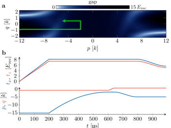
Figure 6: Momentum state preparation. a. Theoretical variation of the energy gap with momentum, and sketch of the momentum ramp used to prepare an arbitrary state (green arrow). It avoids crossing the lines of small energy gaps (in white) occurring in the edge mode region. b. Time evolution of the light couplings $t_{x}$, $t_{z}$ and momentum components $p$, $q$ for the adiabatic preparation of a given momentum state.

Preparation of arbitrary momentum states
The atomic gas is initially prepared in a crossed optical dipole trap (oscillation frequencies $\omega_{x}=2\pi\times$263(5)\text{\,}\mathrm{Hz}$$ and $\omega_{z}=2\pi\times$140(6)\text{\,}\mathrm{Hz}$$), at a sub-recoil temperature $T=$260(10)\text{\,}\mathrm{nK}$$ using standard cooling techniques. The atoms are subjected to a magnetic field $B=$221(1)\text{\,}\mathrm{m}\mathrm{G}$$ along $z$, producing a linear Zeeman splitting between the magnetic sub-levels $m$ of frequency $\omega_{\text{Z}}=2\pi\times$385(3)\text{\,}\mathrm{kHz}$$. At this stage, the atoms are fully-polarized in the ground state $m=-J$.

The preparation of a given momentum state dressed by the Raman lasers proceeds as follows. We switch off the optical dipole trap, and increase the Raman laser intensities to $t_{x}=8.2(1)\,E_{\text{rec}}$ and $t_{z}=7.4(1)\,E_{\text{rec}}$ in $200\text{\,}\mathrm{\SIUnitSymbolMicro s}$. During this process, the Raman lasers are off-resonant, with frequency detunings $\delta_{x}=-\delta_{z}/2=14.9(2)\,E_{\text{rec}}$ corresponding to momentum components $p=-15.5(1)\,k$ and $q=-2k/\sqrt{5}\simeq-0.89\,k$. For this momentum, the ground state matches the initial spin polarization in $m=-J$. We then ramp the detunings towards resonance, leading to an inertial force when considering the atoms in the moving frame as discussed above. The preparation of given p states is based on momentum trajectories as pictured in Fig. 6a. We first increase the momentum to $p=-2\,k$ in the bulk mode region, then ramp the quasi-momentum $q$, followed by a variation of $p$ to the final value. We finally decrease the spin coupling amplitudes to $t_{x}=5.69(6)\,E_{\text{rec}}$ and $t_{z}=5.1(1)\,E_{\text{rec}}$. This protocol minimizes the crossing of small energy gaps separating the ground and first excited bands in the edge mode region. The duration of detuning ramps, displayed in Fig. 6b, is chosen as a compromise between the adiabaticity requirement and the effect of dipolar relaxation, which leads to heating of the sample and atom loss on a $10\text{\,}\mathrm{ms}$ timescale.

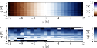
Figure 7: Momentum projections. Measurement of the mean momentum components $\langle p\rangle$ (a) and $\langle q\rangle$ (b) of a thermal gas as a function of the targeted momentum.

We show in Fig. 7 a comparison between measured and targeted momenta across the Brillouin zone. The small discrepancy between theory and experiment can be attributed to the confinement induced by the Raman lasers and gravity, which provide an additional small contribution to the momentum dynamics. This effect does not play a role in our data analysis, as explained in the next section.

Atom imaging and data analysis
At the end of the experimental sequence, the light beams are switched off and the atoms are let to expand for a duration of $2.4\text{\,}\mathrm{ms}$ before an absorption image is taken. During expansion, a magnetic field gradient is applied, leading to a spatial separation of the different magnetic sub-levels $m$ along $z$. The measured atom density thus gives access to the velocity distribution $\mathcal{D}_{\textbf{p}}(m,\textbf{v})$, resolved in magnetic projection $m$, for the prepared momentum state p. An example of an absorption image is shown in Fig. 8.

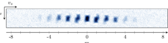
Figure 8: Typical absorption image. Absorption image of an atomic sample of mean momentum $\langle\textbf{p}\rangle\simeq 0$ and thermal width $\sigma_{p}=1.4(1)k$. The sample is split between the $2J+1$ magnetic sub-levels by a magnetic field gradient. For each magnetic projection, the density profile, taken after time-of-flight, provides the velocity distribution in the $xz$ plane.

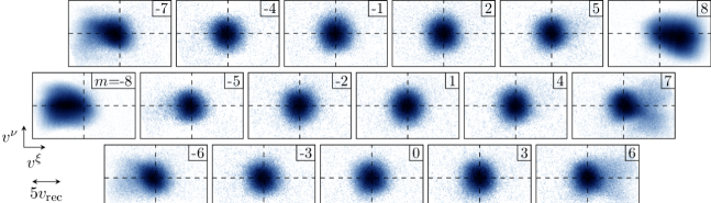
Figure 9: Density of states. Density of states $\mathcal{D}(m,\textbf{v})$ of the ground band as a function of the magnetic projection $m$ and the velocity v. Each panel corresponds to a given $m$ component. The density of states is obtained by integrating the spin-resolved velocity distributions over the momentum interval $|p|\leq 12k$. The dashed lines indicate $v^{\xi}=0$ and $v^{\nu}=0$. This data is used for the generation of Fig. 2 and 3.

The thermal momentum width $\sigma_{p}=1.4(1)k$ after loading in the ground band ($\sigma_{p}=0.9(1)k$ prior to loading) leads to an averaging of the measured spin-resolved velocity distribution around a mean value $\langle\textbf{p}\rangle$. However, a given momentum state expands on a discrete set of velocities as $M\textbf{v}=\textbf{p}-2km\hat{\textbf{x}}+\ell\textbf{K}$, with $\ell$ integer. Different momentum states thus contribute to separate components of the velocity distribution, which allows us to deconvolve the thermal broadening and reconstruct the velocity distribution for each momentum value. In order to treat all momenta on equal footing, we sum the spin-resolved velocity distributions measured for a dense sample of momenta $\langle\textbf{p}\rangle$ within the Brillouin zone, before performing the momentum deconvolution. Averaging all momenta before deconvolution also suppresses the effect of residual forces, such as gravity and laser beam confinement, occurring during the state preparation. The integrated distribution $\mathcal{D}(m,\textbf{v})=\int\text{d}\textbf{p}\,\mathcal{D}_{\textbf{p}}(m,\textbf{v})$, plotted in Fig. 9, physically corresponds to the spin-velocity density of states of the ground band.

The spin-resolved velocity distributions $\mathcal{D}_{\textbf{p}}(m,\textbf{v})$ give direct access to the spin projection probabilities $\Pi_{m}$ and mean velocities $\langle\textbf{v}\rangle$, plotted in Fig. 2. The mean spin projection is then given by

$$\langle m\rangle\equiv\sum_{m}\Pi_{m}m.$$

The mean value of the cyclic variable $n$ is a priori ill-defined [37]. However, since we observe a peaked probability distribution in $n$, we track the dynamics along $n$ from the following estimate of the mean position

$$\langle n\rangle\equiv\frac{2}{3\pi}\arg\left<\exp\left(\text{i}\frac{2\pi}{3}m\right)\right>.$$

Response to a force along $m$
The measurement of the bulk Berry curvature presented in the main text relies on the application of a force in the $xy$ plane, leading to a Hall drift along $n$ and $m$. In order to access the Berry curvature component $\Omega^{\text{bulk}}_{nm}$, we consider a force applied along $m$, which is equivalent to a perturbative Zeeman field $\hbar\Delta J_{z}$. This field can be produced by additional detunings of the Raman transitions $\delta_{x}=-\Delta$ and $\delta_{z}=2\Delta$. The gauge transform $U=\exp(\text{i}\Delta tJ_{z})$ suppresses the time-dependency while adding the desired Zeeman field $\hbar\Delta J_{z}$. As explained earlier, shifts in detuning can also be interpreted as a shift in momentum p. A perturbative Zeeman energy is thus equivalent to a variation of momentum within the ground band. Since all momentum states of the ground band are characterized by static spin distributions, we conclude the absence of velocity along $n$ induced by the force along $m$, hence $\Omega^{\text{bulk}}_{nm}=0$.

Berry curvature measurements
The second Chern character plotted in Fig. 5a is obtained as a non-linear combination of Berry curvatures. In this section we show that the latter can be expressed in terms of p-variations of the measured mean velocity $\langle\textbf{v}\rangle(\textbf{p})$ (Fig. 2d).

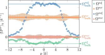
Figure 10: Berry curvature. Berry curvature components $\Omega^{\alpha\beta}$ computed from the measurements of the mean velocity. The measured values are independent on the quasi-momentum $q$ within error bars, and we show the $q$-averaged value $\langle\Omega^{\alpha\beta}\rangle_{q}$ as a function of the momentum $p$. The solid line are the components of the bulk Berry curvature $\bm{\Omega}_{\text{bulk}}$ given by (5).

We consider an atom initially occupying a momentum state p. The Berry curvature $\Omega^{\alpha\beta}(\textbf{p})$ quantifies its linear response in velocity $\delta v^{\alpha}$ following a perturbative variation of an external gauge field $\delta\dot{A}_{\beta}$, as

$$\Omega^{\alpha\beta}=-\frac{\delta\langle v^{\alpha}\rangle}{\delta\dot{A}_{\beta}}.$$

We assume a time-dependent gauge field $\dot{\delta A_{n}}$ along $n$ and $\dot{\delta A_{m}}$ along $m$, corresponding to Peierls phases

$$\phi_{x} =-2kx+(\delta\dot{A}_{n}+\delta\dot{A}_{m})t,$$

$$\phi_{z} =-2kz+(\delta\dot{A}_{n}-2\delta\dot{A}_{m})t.$$

The time dependency can be eliminated by considering the atom in a reference frame moving at velocity

$$\delta\textbf{u} =\frac{\delta\dot{A}_{n}(\hat{\textbf{x}}+\hat{\textbf{z}})+\dot{\delta A_{m}}(\hat{\textbf{x}}-2\hat{\textbf{z}})}{2k}$$

$$=\frac{\delta\dot{A}_{n}}{2\sqrt{5}k}(-\hat{\bm{\xi}}+3\hat{\bm{\nu}})+\frac{\sqrt{5}\dot{\delta A_{m}}}{2k}\hat{\bm{\xi}}.$$

In that frame, the atom occupies the state of momentum $\textbf{p}-M\delta\textbf{u}$ and velocity $\langle\textbf{v}\rangle(\textbf{p}-M\delta\textbf{u})$. Coming back to the original reference frame, the change of mean velocity due to the gauge field variation writes

$$\delta\langle\textbf{v}\rangle =\langle\textbf{v}\rangle(\textbf{p}-M\delta\textbf{u})+\delta\textbf{u}$$

$$=\frac{\delta\dot{A}_{n}}{2\sqrt{5}k}\left(-\hat{\bm{\xi}}+3\hat{\bm{\nu}}+M\frac{\partial\langle\textbf{v}\rangle}{\partial p}-3M\frac{\partial\langle\textbf{v}\rangle}{\partial q}\right)$$

$$\;\;\;\;+\frac{\sqrt{5}\dot{\delta A_{m}}}{2k}\left(\hat{\bm{\xi}}-M\frac{\partial\langle\textbf{v}\rangle}{\partial p}\right).$$

Taking the $\xi$- and $\nu$-projections of this expansion yields the Berry curvature components

$$\Omega^{\xi n} =\frac{1}{2\sqrt{5}k}\left(1-M\frac{\partial\langle v^{\xi}\rangle}{\partial p}+3M\frac{\partial\langle v^{\xi}\rangle}{\partial q}\right),$$

$$\Omega^{\nu n} =\frac{1}{2\sqrt{5}k}\left(-3-M\frac{\partial\langle v^{\nu}\rangle}{\partial p}+3M\frac{\partial\langle v^{\nu}\rangle}{\partial q}\right),$$

$$\Omega^{\xi m} =\frac{\sqrt{5}}{2k}\left(-1+M\frac{\partial\langle v^{\xi}\rangle}{\partial p}\right),$$

$$\Omega^{\nu m} =\frac{\sqrt{5}}{2k}M\frac{\partial\langle v^{\nu}\rangle}{\partial p}.$$

We use these expressions to compute the Berry curvature tensor from the measurements of the mean velocity $\langle\textbf{v}\rangle(\textbf{p})$. Our data, shown in Fig. 10, is consistent with the expected Berry curvature $\Omega_{\text{bulk}}$ in the bulk mode region of the Brillouin zone.

Effective continuous model in the bulk
Derivation of the continuous model
The cyclotron dynamics in the bulk of our system can be modeled using a simple effective model of a charged particles evolving in 4D and subjected to a magnetic field. In the Hamiltonian (1), we replace spin ladder operators by translation operators along $m$ and $n$, expressed in terms of momentum operators $p_{m}$ and $p_{n}$ as

$$J_{+} =\exp[-\text{i}(p_{m}+p_{n})]\sqrt{J(J+1)-m(m+1)}$$

$$\simeq(J-m^{2}/2J)\exp[-\text{i}(p_{n}+p_{m})],$$

where we assume $|m|\ll J$, and only kept the lowest order in $1/J$. Similarly, we obtain for the second-order spin transition

$$J_{-}^{2}\simeq(J^{2}-m^{2})\exp[-\text{i}(p_{n}-2p_{m})].$$

The Hamiltonian then writes

$$H= \frac{Mv^{2}}{2}-\bigg{(}t_{x}\text{e}^{\text{i}\phi_{x}}\frac{J_{+}}{J}+t_{z}\text{e}^{\text{i}\phi_{z}}\frac{J_{-}^{2}}{J^{2}}+\text{hc}\bigg{)}+\beta\frac{J_{z}^{2}}{J^{2}}$$

$$\simeq \,\frac{p_{x}^{2}+p_{z}^{2}}{2M}-\bigg{[}t_{x}\left(1-\frac{1}{2}\left(\frac{m}{J}\right)^{2}\right)\text{e}^{-\text{i}(p_{n}+p_{m}-2kx)}$$

$$+t_{z}\left(1-\left(\frac{m}{J}\right)^{2}\right)\text{e}^{-\text{i}(p_{n}-2p_{m}-2kz)}+\text{hc}\bigg{]}+\beta\left(\frac{m}{J}\right)^{2}.$$

Expanding it up to quadratic order in all dynamical variables, we obtain

$$H \simeq\epsilon_{0}+H_{\text{kin}}+\beta^{\prime}\left(\frac{m}{J}\right)^{2},$$

$$\epsilon_{0} =-2t_{x}-2t_{z},$$

$$H_{\text{kin}} =\frac{p_{x}^{2}+p_{z}^{2}}{2M}+t_{x}(p_{n}+p_{m}-2kx)^{2}$$

$$\phantom{=\;}+t_{z}(p_{n}-2p_{m}-2kz)^{2},$$ (7)

$$\beta^{\prime} =\beta+t_{x}+2t_{z}.$$

The energy $\epsilon_{0}$ is a mere energy shift playing no role in the atom dynamics. Reminding that $\beta=-2t_{z}$, we are left with a residual Zeeman shift $\beta^{\prime}=t_{x}$ that explains the residual positive energy curvature in the bulk of the dispersion relation (Fig. 1d).

Generalized Landau levels
The kinetic energy can be recast as

$$H_{\text{kin}}=\frac{1}{2}\left(\frac{1}{M}\right)^{\alpha\beta}(p_{\alpha}-A_{\alpha})(p_{\beta}-A_{\beta}),$$ (8)

where the vector potential

$$\textbf{A}=\frac{-2k}{3}(0,0,2x+z,x-z)$$

and its associated magnetic field

$$\textbf{B}=\frac{2k}{3}\begin{pmatrix}0&0&-2&-1\\ 0&0&-1&1\\ 2&1&0&0\\ 1&-1&0&0\end{pmatrix}$$

were already introduced in the main text. The inverse mass tensor is given by

$$\frac{1}{\textbf{M}}=\begin{pmatrix}1/M&0&0&0\\ 0&1/M&0&0\\ 0&0&2t_{x}+2t_{z}&2t_{x}-4t_{z}\\ 0&0&2t_{x}-4t_{z}&2t_{x}+8t_{z}\end{pmatrix}.$$

Considered alone, the kinetic Hamiltonian $H_{\text{kin}}$ describes the motion of a charged particle of anisotropic mass and subjected to a magnetic field in 4D. The momenta $p_{m}$ and $p_{n}$ are conserved quantities and the $x$ and $z$ motions map to independent harmonic oscillators of frequencies

$$\omega_{x}=4\sqrt{E_{\text{rec}}t_{x}},\quad\omega_{z}=4\sqrt{E_{\text{rec}}t_{z}}.$$ (9)

The harmonic energy spectrum $E_{n_{x},n_{z}}=\omega_{x}(n_{x}+\tfrac{1}{2})+\omega_{z}(n_{z}+\tfrac{1}{2})$ corresponds to the direct sum of Landau levels with macroscopic degeneracy indexed by $p_{m}$ and $p_{n}$. For the couplings $t_{x}=5.69(6)\,E_{\text{rec}}$ and $t_{z}=5.1(1)\,E_{\text{rec}}$ used in our experiments, the expressions (9) yield $\omega_{x}=2\pi\times$30.2(2)\text{\,}\mathrm{kHz}$$ and $\omega_{z}=2\pi\times$28.4(3)\text{\,}\mathrm{kHz}$$, close to the frequencies computed from the actual Hamiltonian (1), namely $\omega_{x}=2\pi\times$27.4(2)\text{\,}\mathrm{kHz}$$ and $\omega_{z}=2\pi\times$26.5(3)\text{\,}\mathrm{kHz}$$.

Band dispersion due to the quadratic Zeeman shift
When including the quadratic Zeeman shift $\beta^{\prime}(m/J)^{2}$, the momentum $p_{m}$ is no longer conserved. To retrieve the energy spectrum in a simple manner, we perform a gauge transform of unitary

$$U=\exp\left(\frac{2k}{3}\left[(2x+z)n+(x-z)m\right]\right),$$

leading to a new Hamiltonian

$$H =\epsilon_{0}+\;\frac{1}{2M}\left(p_{x}-\frac{2k}{3}(2n+m)\right)^{2}$$

$$+\frac{1}{2M}\left(p_{z}-\frac{2k}{3}(n-m)\right)^{2}$$

$$+t_{x}(p_{n}+p_{m})^{2}+t_{z}(p_{n}-2p_{m})^{2}+\beta^{\prime}\left(\frac{m}{J}\right)^{2}.$$ (10)

This Hamiltonian conserves the momenta $p_{x}$ and $p_{z}$. The $m$ and $n$ dynamics is quadratic, such as it is straightforward to compute the energy spectrum, as

$$E_{n_{x},n_{z}}(p)=\epsilon_{0}+\omega_{x}(n_{x}+\tfrac{1}{2})+\omega_{z}(n_{z}+\tfrac{1}{2})+\frac{5\beta^{\prime}}{4J^{2}}\left(\frac{p}{k}\right)^{2}.$$

where $p$ is the momentum component along $\hat{\bm{\xi}}$ and we assumed $\beta^{\prime}\ll J^{2}E_{\text{rec}}$ for simplicity. This expression explains the $p$ curvature of the ground band shown in Fig. 1d, while the bulk spectrum is essentially flat along $q$.

Equations of motion
The continuous model can also be used to compute the cyclotron dynamics. For simplicity, we restrict the dynamics to the kinetic Hamiltonian (10), and obtain the equations of motion

$$\partial_{t}v^{\alpha}=\left(\frac{1}{M}\right)^{\alpha\beta}B_{\beta\gamma}v^{\gamma},$$

explicitely given by

$$\partial_{t}\begin{pmatrix}v_{x}\\ v_{z}\\ v_{n}\\ v_{m}\end{pmatrix}\!=\!\begin{pmatrix}0&0&-4v_{\text{rec}}/3&-2v_{\text{rec}}/3\\ 0&0&-2v_{\text{rec}}/3&2v_{\text{rec}}/3\\ 4kt_{x}&4kt_{z}&0&0\\ 4kt_{x}&-8kt_{z}&0&0\\ \end{pmatrix}\!\begin{pmatrix}v_{x}\\ v_{z}\\ v_{n}\\ v_{m}\end{pmatrix}\!.$$

The dynamics in the $xz$ plane can be expressed in a closed manner as

$$\partial_{t}^{2}\begin{pmatrix}v_{x}\\ v_{z}\end{pmatrix} =\begin{pmatrix}-4v_{\text{rec}}/3&-2v_{\text{rec}}/3\\ -2v_{\text{rec}}/3&2v_{\text{rec}}/3\end{pmatrix}\begin{pmatrix}4kt_{x}&4kt_{z}\\ 4kt_{x}&-8kt_{z}\end{pmatrix}\begin{pmatrix}v_{x}\\ v_{z}\end{pmatrix}$$

$$=-\begin{pmatrix}\omega_{x}^{2}&0\\ 0&\omega_{z}^{2}\end{pmatrix}\begin{pmatrix}v_{x}\\ v_{z}\end{pmatrix},$$

describing harmonic motion along $x$ and $z$ of frequencies $\omega_{x}$ and $\omega_{z}$ given by (9).

Foucault pendulum precession from a $b_{nm}$ field
We investigate the effect of a magnetic perturbation $b_{nm}$ in the $nm$ plane within the frame of the continuous model described above. The $b_{nm}$ field is induced by an additional phase factor in the $x$-Raman transitions $\phi_{x}^{\prime}=-\tfrac{3}{2}b_{nm}m$, such that the vector potential becomes

$$\textbf{A}=\left(\!0,0,\frac{-2k}{3}(2x+z)-b_{nm}m,\frac{-2k}{3}(x-z)-\frac{1}{2}b_{nm}m\!\right)\!,$$

yielding a magnetic field

$$\textbf{B}=\begin{pmatrix}0&0&-\frac{4k}{3}&-\frac{2k}{3}\\ 0&0&-\frac{2k}{3}&\frac{2k}{3}\\ \frac{4k}{3}&\frac{2k}{3}&0&b_{nm}\\ \frac{2k}{3}&-\frac{2k}{3}&-b_{nm}&0\end{pmatrix}$$

and equations of motion

$$\partial_{t}\begin{pmatrix}v_{x}\\ v_{z}\\ v_{n}\\ v_{m}\end{pmatrix}=$$

$$\!\begin{pmatrix}0&0&-4v_{\text{rec}}/3&-2v_{\text{rec}}/3\\ 0&0&-2v_{\text{rec}}/3&2v_{\text{rec}}/3\\ 4kt_{x}&4kt_{z}&-2b_{nm}(t_{x}-2t_{z})&-2b_{nm}(t_{x}+t_{z})\\ 4kt_{x}&-8kt_{z}&2b_{nm}(t_{x}+4t_{z})&2b_{nm}(t_{x}-2t_{z})\\ \end{pmatrix}\!\!\!\begin{pmatrix}v_{x}\\ v_{z}\\ v_{n}\\ v_{m}\end{pmatrix}\!\!.$$

In order to obtain a closed equation for the dynamics in the $xz$ plane, we invert the relation

$$\partial_{t}\begin{pmatrix}v_{x}\\ v_{z}\end{pmatrix}=\frac{2v_{\text{rec}}}{3}\begin{pmatrix}-2&-1\\ -1&1\end{pmatrix}\begin{pmatrix}v_{n}\\ v_{m}\end{pmatrix}$$

as

$$\begin{pmatrix}v_{n}\\ v_{m}\end{pmatrix}=\frac{1}{2v_{\text{rec}}}\begin{pmatrix}-1&-1\\ -1&2\end{pmatrix}\partial_{t}\begin{pmatrix}v_{x}\\ v_{z}\end{pmatrix}.$$

This allows us to eliminate the $m$ and $n$ velocities and obtain closed dynamics equations along $x$ and $z$, as

$$\partial_{t}^{2}v_{x} =-\omega_{x}^{2}(v_{x}+M\rho_{2}^{\text{bulk}}\partial_{t}v_{z}),$$

$$\partial_{t}^{2}v_{z} =-\omega_{z}^{2}(v_{z}-M\rho_{2}^{\text{bulk}}\partial_{t}v_{x}),$$

involving the bulk second Chern character $\rho_{2}^{\text{bulk}}=3/4k^{2}$.

The Foucault pendulum precession occurs for equal frequencies $\omega_{x}=\omega_{z}=\omega$, leading to an $xz$ dynamics

$$\partial_{t}^{2}\textbf{v}=-\omega^{2}\textbf{v}+2\omega_{\text{p}}\hat{\textbf{n}}\times\textbf{v},$$

$\hat{\textbf{n}}=\hat{\textbf{x}}\times\hat{\textbf{z}}$ is normal to the $xz$ plane. We recognize the equation of motion of a Foucault pendulum of harmonic frequency $\omega$ and precession rate $\omega_{\text{p}}$ given by (6) in the main text.

This connection between the precession rate $\omega_{\text{p}}$ and the second Chern character $\rho_{2}^{\text{bulk}}$ is not specific to the precise algebra of our setting, and would apply for arbitrary implementations of a 4D quantum Hall system using an artificial magnetic field.

The non-linear electromagnetic response could in principle be measured more directly, from the geometrical drift induced by both a force $f_{x}$ along $x$ and a magnetic perturbation $b_{nm}$, as

$$\langle z\rangle_{\text{non-linear}}(t)=-\rho_{2}b_{nm}f_{x}t.$$ (11)

For the $b_{nm}$ field accessible in our setting, we expect a displacement $\delta z\simeq$5\text{\,}\mathrm{nm}$$ for an experiment duration $t=k/f_{x}$ such that the force $f_{x}$ changes the momentum by $k$. This displacement is too small to be accessible in our setting. We note that the $b_{nm}$ field used in our experiments is already at the limit of validity of the linear response given by (11).

Local second Chern marker
The occurrence of edge states in our system implies the absence of a gap in the energy spectrum, such that the system as a whole is not topological (Fig. 1d). Nevertheless, the lowest band features a weak dispersion and a bulk energy gap, such that non-trivial topological properties are expected when probing the bulk only. To access it, we consider the local second Chern marker, defined as [38, 39]

$$C_{2}(\textbf{r})=2\pi^{2}\epsilon_{\alpha\beta\delta\gamma}\langle\textbf{r}|Pr^{\alpha}Pr^{\beta}Pr^{\delta}Pr^{\gamma}P|\textbf{r}\rangle,$$

where $P$ projects on the lowest Bloch band. For an infinite and homogeneous system, it coincides with the integer second Chern number $\mathcal{C}_{2}$. In a finite system with open boundaries, we expect $C_{2}(\textbf{r})$ to match $\mathcal{C}_{2}$ for positions r within the bulk only [38].

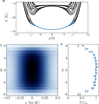
Figure 11: Local second Chern marker. a. Dispersion relation computed for the parameters used in the experiment. The calculation of $C_{2}(\nu,m)$ involves all states of the ground band in the interval $(-p^{\star},p^{\star})$, with $p^{\star}=7k$, discarding strongly dispersive edge modes. b. Local second Chern marker $C_{2}$ plotted as a function of $\nu$ and $m$. c. $\nu$-average of $C_{2}$ as a function of $m$, compared to the experimental data (dots).

For our system, this marker can be rewritten in terms of accessible observables as follows [40]. We decompose the band projector $P=\int\text{d}p\,\text{d}q\left|\psi_{pq}\right>\left<\psi_{pq}\right|$ on magnetic Bloch states $\left|\psi_{pq}\right>$, such that the Chern marker writes

$$C_{2}(\textbf{r}) =2\pi^{2}\epsilon_{\alpha\beta\delta\gamma}\int\text{d}p_{1}\,\text{d}q_{1}\,\text{d}p_{2}\,\text{d}q_{2}\,\text{d}p_{3}\,\text{d}q_{3}$$

$$\;\;\;\;\;\;\;\;\;\;\psi_{p_{1}q_{1}}^{*}(\textbf{r})\psi_{p_{2}q_{2}}(\textbf{r})c^{\alpha\beta}_{p_{1}q_{1}p_{3}q_{3}}c^{\delta\gamma}_{p_{3}q_{3}p_{2}q_{2}},$$ (12)

$$c^{\alpha\beta}_{p_{1}q_{1}p_{2}q_{2}} \equiv\langle\psi_{p_{1},q_{1}}|r^{\alpha}Pr^{\beta}|\psi_{p_{2},q_{2}}\rangle.$$

The coefficient involving $\xi$ and $m$ directions reads

$$c^{\xi m}_{p_{1}q_{1}p_{2}q_{2}}=\text{i}\langle m\rangle_{p_{2}q_{2}}\langle\psi_{p_{1}q_{1}}|\psi_{p_{2}q_{2}}\rangle\delta^{\prime}(p_{1}-p_{2})\delta(q_{1}-q_{2}),$$

and similar expressions can be written for other coefficients $c^{\alpha\beta}_{p_{1}q_{1}p_{2}q_{2}}$. Injecting these expressions in (12), we obtain

$$C_{2}(\textbf{r})=4\pi^{2}\!\!\int\!\text{d}p\,\text{d}q\,|\psi_{pq}(\textbf{r})|^{2}(\partial_{p}\langle m\rangle\partial_{q}\langle n\rangle-\partial_{q}\langle m\rangle\partial_{p}\langle n\rangle).$$

We recognize the Berry curvature components, e.g. $\Omega^{m\xi}=\partial_{p}\langle m\rangle$, such that their non-linear combination matches the second Chern character $\rho_{2}$, leading to

$$C_{2}(\textbf{r})=4\pi^{2}\int\text{d}p\,\text{d}q\,|\psi_{pq}(\textbf{r})|^{2}\rho_{2}(p,q).$$

The system is transitionally invariant along $\xi$, and exhibits a discrete translation symmetry along $\nu$ of reciprocal lattice vector K. We thus expect the local second Chern character to depend on $\nu$ and $m$ only. Since the $\nu$ modulation occurs on a small length scale $1/K$ only, we define the $\nu$ coarse average $\langle C_{2}\rangle_{\nu}(m)$, involving the $m$-projection probability $\Pi_{m}$ only, as

$$\langle C_{2}\rangle_{\nu}(m)=\frac{1}{3}\int\text{d}p\,\text{d}q\,\Pi_{m}(p,q)\rho_{2}(p,q).$$

The integration should be performed on bulk modes only, defined by the interval $|p|<p^{*}$. The momentum cutoff $p^{*}=7k$ is chosen such that the ground band energy approximately reaches at $p^{*}$ the middle of the bulk gap between the ground and first excited bands (Fig. 11a). The precise choice of $p^{\star}$ does not significantly influence the values of $\langle C_{2}\rangle_{\nu}(m)$ in the bulk of the system.

We show in Fig. 11b the local second Chern marker $C_{2}(\nu,m)$, numerically computed for the coupling parameters used in the experiment. Its $\nu$-average $\langle C_{2}\rangle_{\nu}(m)$ is very close to the second Chern number $\mathcal{C}_{2}=1$ in the bulk $|m|\lesssim 5$, and agrees well with our measurements (Fig. 11c).

Acknowledgements
We thank Jean Dalibard for insightful discussions and careful reading of the manuscript. This work is supported by European Union (grant TOPODY 756722 from the European Research Council) and Institut Universitaire de France.

Author contributions
All authors contributed to the set-up of the experiment, data acquisition, data analysis and the writing of the manuscript.

Competing interests
The authors declare no competing interests.

Data availability
Source data, as well as other datasets generated and analysed during the current study, are available from the corresponding author upon request.

References

v. Klitzing et al. [1980]K. v. Klitzing, G. Dorda, and M. Pepper, New Method for High-Accuracy
Determination of the Fine-Structure Constant Based on Quantized Hall
Resistance, Phys. Rev. Lett. 45, 494 (1980).
Thouless et al. [1982]D. J. Thouless, M. Kohmoto,
M. P. Nightingale, and M. den Nijs, Quantized Hall Conductance in a
Two-Dimensional Periodic Potential, Phys. Rev. Lett. 49, 405 (1982).
Halperin [1982]B. I. Halperin, Quantized Hall
conductance, current-carrying edge states, and the existence of extended
states in a two-dimensional disordered potential, Phys. Rev. B 25, 2185 (1982).
Hsieh et al. [2008]D. Hsieh, D. Qian,
L. Wray, Y. Xia, Y. S. Hor, R. J. Cava, and M. Z. Hasan, A topological
Dirac insulator in a quantum spin Hall phase, Nature 452, 970 (2008).
Lu et al. [2015]L. Lu, Z. Wang, D. Ye, L. Ran, L. Fu, J. D. Joannopoulos, and M. Soljačić, Experimental observation of Weyl points, Science 349, 622 (2015).
Xu et al. [2015]S.-Y. Xu, I. Belopolski,
N. Alidoust, M. Neupane, G. Bian, C. Zhang, R. Sankar, G. Chang, Z. Yuan, C.-C. Lee, S.-M. Huang, H. Zheng,
J. Ma, D. S. Sanchez, B. Wang, A. Bansil, F. Chou, P. P. Shibayev, H. Lin, S. Jia, and M. Z. Hasan, Discovery of a Weyl fermion semimetal and
topological Fermi arcs, Science 349, 613 (2015).
Ryu et al. [2010]S. Ryu, A. P. Schnyder,
A. Furusaki, and A. W. W. Ludwig, Topological insulators and
superconductors: Tenfold way and dimensional hierarchy, New J. Phys. 12, 065010 (2010).
Fröhlich and Pedrini [2000]J. Fröhlich and B. Pedrini, New applications of the
chiral anomaly, in Mathematical Physics 2000 (World
Scientific, 2000) pp. 9–47.
Zhang and Hu [2001]S.-C. Zhang and J. Hu, A Four-Dimensional Generalization
of the Quantum Hall Effect, Science 294, 823 (2001).
Lohse et al. [2018]M. Lohse, C. Schweizer,
H. M. Price, O. Zilberberg, and I. Bloch, Exploring 4D quantum Hall physics with a 2D
topological charge pump, Nature 553, 55 (2018).
Zilberberg et al. [2018]O. Zilberberg, S. Huang,
J. Guglielmon, M. Wang, K. P. Chen, Y. E. Kraus, and M. C. Rechtsman, Photonic topological boundary pumping as a probe of 4D
quantum Hall physics, Nature 553, 59 (2018).
Wang et al. [2020]Y. Wang, H. M. Price,
B. Zhang, and Y. D. Chong, Circuit implementation of a four-dimensional topological
insulator, Nat
Commun 11, 2356
(2020).
Celi et al. [2014]A. Celi, P. Massignan,
J. Ruseckas, N. Goldman, I. B. Spielman, G. Juzeliūnas, and M. Lewenstein, Synthetic Gauge Fields in Synthetic Dimensions, Phys. Rev. Lett. 112 (2014).
Mancini et al. [2015]M. Mancini, G. Pagano,
G. Cappellini, L. Livi, M. Rider, J. Catani, C. Sias, P. Zoller, M. Inguscio,
M. Dalmonte, and L. Fallani, Observation of chiral edge states with neutral
fermions in synthetic Hall ribbons, Science 349, 1510 (2015).
Stuhl et al. [2015]B. K. Stuhl, H.-I. Lu,
L. M. Aycock, D. Genkina, and I. B. Spielman, Visualizing edge states with an atomic Bose gas in the
quantum Hall regime, Science 349, 1514 (2015).
Bernevig et al. [2002]B. A. Bernevig, C.-H. Chern,
J.-P. Hu, N. Toumbas, and S.-C. Zhang, Effective Field Theory Description of the Higher Dimensional
Quantum Hall Liquid, Annals of Physics 300, 185 (2002).
Yang and Mills [1954]C. N. Yang and R. L. Mills, Conservation of Isotopic
Spin and Isotopic Gauge Invariance, Phys. Rev. 96, 191 (1954).
Barns-Graham et al. [2018]A. Barns-Graham, N. Dorey, N. Lohitsiri,
D. Tong, and C. Turner, ADHM and the 4d quantum Hall effect, J. High Energ. Phys. 2018, 40.
Bansil et al. [2016]A. Bansil, H. Lin, and T. Das, Colloquium : Topological band
theory, Rev.
Mod. Phys. 88 (2016).
Ozawa and Price [2019]T. Ozawa and H. M. Price, Topological quantum matter
in synthetic dimensions, Nat. Rev. Phys. 1, 349 (2019).
Kraus et al. [2013]Y. E. Kraus, Z. Ringel, and O. Zilberberg, Four-Dimensional Quantum Hall Effect in a
Two-Dimensional Quasicrystal, Phys. Rev. Lett. 111, 226401 (2013).
Price et al. [2015]H. M. Price, O. Zilberberg,
T. Ozawa, I. Carusotto, and N. Goldman, Four-Dimensional Quantum Hall Effect with Ultracold
Atoms, Phys.
Rev. Lett. 115, 195303
(2015).
Ozawa et al. [2016]T. Ozawa, H. M. Price,
N. Goldman, O. Zilberberg, and I. Carusotto, Synthetic dimensions in integrated photonics: From
optical isolation to four-dimensional quantum Hall physics, Phys. Rev. A 93, 043827 (2016).
Qi et al. [2008]X.-L. Qi, T. L. Hughes, and S.-C. Zhang, Topological field theory of
time-reversal invariant insulators, Phys. Rev. B 78, 195424 (2008).
Yang [1978]C. N. Yang, Generalization of
Dirac’s monopole to SU2 gauge fields, J. Math. Phys. 19, 320 (1978).
Sugawa et al. [2018]S. Sugawa, F. Salces-Carcoba, A. R. Perry, Y. Yue, and I. B. Spielman, Second Chern number of a
quantum-simulated non-Abelian Yang monopole, Science 360, 1429 (2018).
Tan et al. [2021]X. Tan, D.-W. Zhang,
W. Zheng, X. Yang, S. Song, Z. Han, Y. Dong, Z. Wang, D. Lan, H. Yan, S.-L. Zhu, and Y. Yu, Experimental
Observation of Tensor Monopoles with a Superconducting Qudit, Phys. Rev. Lett. 126, 017702 (2021).
Chen et al. [2022]M. Chen, C. Li, G. Palumbo, Y.-Q. Zhu, N. Goldman, and P. Cappellaro, A
synthetic monopole source of Kalb-Ramond field in diamond, Science 375, 1017 (2022).
Elvang and Polchinski [2003]H. Elvang and J. Polchinski, The quantum Hall
effect on R4, Comptes Rendus Physique 4, 405 (2003).
Fabre et al. [2022]A. Fabre, J.-B. Bouhiron,
T. Satoor, R. Lopes, and S. Nascimbene, Simulating two-dimensional dynamics within a large-size
atomic spin, Phys. Rev. A 105, 013301 (2022).
Lin et al. [2009]Y.-J. Lin, R. L. Compton,
K. Jiménez-García, J. V. Porto, and I. B. Spielman, Synthetic
magnetic fields for ultracold neutral atoms, Nature 462, 628 (2009).
Estienne et al. [2021]B. Estienne, B. Oblak, and J.-M. Stéphan, Ergodic edge modes in the 4D
quantum Hall effect, SciPost Phys. 11, 016 (2021).
Lian and Zhang [2016]B. Lian and S.-C. Zhang, Five-dimensional
generalization of the topological Weyl semimetal, Phys. Rev. B 94, 041105 (2016).
Lee et al. [2018]C. H. Lee, Y. Wang, Y. Chen, and X. Zhang, Electromagnetic response of quantum Hall systems in dimensions
five and six and beyond, Phys. Rev. B 98, 094434 (2018).
Petrides et al. [2018]I. Petrides, H. M. Price, and O. Zilberberg, Six-dimensional
quantum Hall effect and three-dimensional topological pumps, Phys. Rev. B 98, 125431 (2018).
Nayak et al. [2008]C. Nayak, S. H. Simon,
A. Stern, M. Freedman, and S. Das Sarma, Non-Abelian anyons and topological quantum
computation, Rev. Mod. Phys. 80, 1083 (2008).
Lynch [1995]R. Lynch, The quantum phase problem:
A critical review, Physics Reports 256, 367 (1995).
Bianco and Resta [2011]R. Bianco and R. Resta, Mapping topological order in
coordinate space, Phys. Rev. B 84, 241106
(2011).
Sykes and Barnett [2021]J. Sykes and R. Barnett, Local topological markers
in odd dimensions, Phys. Rev. B 103, 155134 (2021).
Chalopin et al. [2020]T. Chalopin, T. Satoor,
A. Evrard, V. Makhalov, J. Dalibard, R. Lopes, and S. Nascimbene, Probing chiral edge dynamics and bulk topology of a
synthetic Hall system, Nat. Phys. 16, 1017 (2020).