Cosmic evolution and thermal stability of Barrow holographic dark energy in nonflat Friedmann-Robertson-Walker Universe

Abstract

We study the cosmological evolution of a nonflat Friedmann-Robertson-Walker Universe filled by pressureless dark matter and Barrow Holographic Dark Energy (BHDE). The latter is a dark energy model based on the holographic principle with Barrow entropy instead of the standard Bekenstein-Hawking one. By assuming the apparent horizon of the Universe as IR cutoff, we explore both the cases where a mutual interaction between the dark components of the cosmos is absent/present. We analyze the behavior of various model parameters, such as the BHDE density parameter, the equation of state parameter, the deceleration parameter, the jerk parameter and the square of sound speed. We also comment on the observational consistency of our predictions, showing that the interacting model turns out to be favored by recent experimental constraints from Planck+WP+BAO, SNIa+CMB+LSS and Union2 SNIa joint analysis over the non-interacting one. The thermal stability of our framework is finally discussed by demanding the positivity of the heat capacities and compressibilities of the cosmic fluid.

I Introduction

Despite the recent progress at both theoretical and experimental level, there are still several open problems in modern Cosmology Open . Among these, the issue of the observed accelerating expansion of the Universe has been getting greater attention in the last decades Supern ; Supernbis ; Supernter ; Supernquar ; Supernquin , providing one of the most exciting challenges to the Standard Model of particle physics and Cosmology. A widely accepted paradigm to explain this phenomenon is the existence of a mysterious form of energy with negative pressure - the Dark Energy (DE) - which would dominate the energy-matter budget of the present Universe.

An interesting scenario for the quantitative description of DE is Holographic Dark Energy (HDE) Cohen:1998zx ; Horava:2000tb ; Thomas:2002pq ; Li:2004rb ; Hsu:2004ri ; Huang:2004ai ; Wang:2005ph ; Setare:2006sv ; Granda ; Sheykhi:2011cn ; Bamba:2012cp ; Ghaffari:2014pxa ; Wang:2016och ; Moradpour:2020dfm , which proves to be in good agreement with observations Zhang ; Li ; Zhang2 ; Lu . A crucial ingredient of this framework is the application of the holographic principle at cosmological scales. According to this recipe, the total entropy content of the Universe should be proportional to the area of its two-dimensional boundary, similarly to the Bekenstein-Hawking entropy-area law for black holes. Recently, however, it has been argued that quantum-gravitational effects may induce nontrivial fractal features on the black hole structure, leading to a deformed horizon entropy in the form BarrowBH

$$S_{\Delta}\,\propto\,A^{1+\Delta/2}\,,$$ (1)

where $A$ is the area enclosed by the horizon surface. Corrections to the standard entropy-area law are parameterized by the exponent $0\leq\Delta\leq 1$, where $\Delta=0$ recovers the Bekenstein-Hawking limit, while $\Delta=1$ corresponds to the maximal entropy deformation. It is worth noting that upper bounds on $\Delta$ have been derived in different contexts in Anagnostopoulos:2020ctz ; Leon:2021wyx ; Barrow:2020kug ; Jusufi:2021fek ; Dabrowski:2020atl ; Saridakis:2020cqq ; Luciano:2022pzg ; Vagnozzi:2022moj .

Based on the gravity-thermodynamic conjecture GTC , Eq. (1) is commonly adopted also in Cosmology BarSar ; Sheykhi:2021fwh ; Adhikary:2021xym ; Nojiri:2021jxf ; LucLiu ; GhafLuc to derive modified Friedmann equations from the first law of thermodynamics on the apparent horizon of a Friedmann-Robertson-Walker (FRW) Universe. The ensuing framework is referred to as Barrow Holographic Dark Energy (BHDE) and exhibits a richer phenomenology compared to HDE, allowing us to predict effects beyond the domain of the Standard Model of Cosmology for certain values of $\Delta$ (see, for instance, Luciano:2022pzg ).

In line with the above studies, the properties of some DE models have been largely investigated in Radicella ; Mimoso ; MoradInt ; Santos ; Barboza ; Bhandari at thermodynamic level. Specifically, in Barboza the limits imposed by thermodynamics on a DE fluid have been analyzed by considering the heat capacities and compressibilities. On the other hand, in Bhandari the thermal stability criteria have been explored for interacting DE. A similar analysis has been carried out in Abdollah for the case of Tsallis Holographic Dark Energy Tavayef:2018xwx ; Saridakis:2018unr ; Nojiri:2019skr ; DAgostino ; LucGine , which is a generalization of HDE based on the use of nonextensive Tsallis entropy for the horizon degrees of freedom of Universe Cirto . All these studies suggest the existence of an intimate relation between the cosmic expansion of the Universe, the thermodynamic stability conditions and DE candidates, which deserves careful attention.

Starting from the above premises, in this work we examine the cosmic evolution of a nonflat FRW Universe filled by pressureless dark matter and BHDE. By considering the apparent horizon as IR cutoff and assuming a mutual interaction between the dark sectors of the cosmos, we analyze the behavior of various model parameters, such as the BHDE density parameter, the equation of state parameter, the deceleration parameter, the jerk parameter and the square of sound speed. We then discuss the thermal stability of our model by demanding the positivity of the heat capacities and compressibilities of the cosmic fluid.

Some comments are in order here to motivate our study: first, we emphasize that in the absence of a fully consistent theory of quantum gravity, BHDE represents a first, naive approach to accommodate quantum-gravity corrections within the HDE framework based on simple physical principles BarSar . Furthermore, the usage of the apparent horizon as IR cutoff is substantiated by the fact that, unlike the event horizon, this boundary is consistent with the generalized second law of thermodynamics She1 ; She2 . Last but not least, although it is commonly believed that inflation washed out curvature inhomogeneities in the early Universe, observational evidences suggest that there is still room for a small but non-negligible spatial curvature Chernin ; Ellis ; PLB ; Divale . This is why we consider a nonflat FRW Universe as background for our analysis.

The remainder of the work is organized as follows: in the next section we briefly review the theoretical framework of BHDE. The evolution of the characteristic model parameters is studied in Sec. III for both the noninteracting and interacting cases. In Sec. IV we discuss the thermal stability of BHDE, while conclusions and outlook are finally summarized in Sec. V. Throughout the work, we use natural units $\hbar=c=k_{B}=G=1$.

II Barrow Holographic Dark Energy: a review

Let us start by briefly reviewing the main features of BHDE. It is well-known that the standard HDE is given by the inequality Wang:2016och

$$\rho_{D}L^{4}\leq S\,,$$ (2)

with the further assumption $S\propto A\propto L^{2}$, where $\rho_{D}$ denotes the dark energy density, while $L$ and $S$ are the horizon length and entropy, respectively.

On the other hand, the usage of Barrow entropy (1) leads to BarSar

$$\rho_{D}=CL^{\Delta-2}\,,$$ (3)

where $C$ is an unknown parameter with dimensions $[L]^{-2-\Delta}$. Notice that, for $\Delta=0$, the above relation reduces to the usual HDE, provided that $C=3c^{2}m_{p}^{2}$, where $m_{p}$ is the reduced Planck mass and $c$ the model parameter.

Now, in a nonflat FRW Universe containing pressureless dark matter and BHDE, the first Friedmann equation takes the form

$$H^{2}+\frac{k}{a^{2}}=\frac{8\pi}{3}\left(\rho_{M}+\rho_{D}\right),$$ (4)

where $a$ is the scale factor, $H\equiv\dot{a}/a$ is the Hubble parameter and the dot denotes derivative with respect to the cosmic time $t$.

We also assume that the apparent horizon of radius

$$\tilde{r}_{A}=\frac{1}{\sqrt{H^{2}+k/a^{2}}}$$ (5)

acts as IR cutoff IRCUT ; IRCUTbis , so that Eq. (3) can be cast as

$$\rho_{D}=C\tilde{r}_{A}^{\Delta-2}\,.$$ (6)

The spatial curvature $k$ takes value $+1,0$ or $-1$, depending on whether the shape of the Universe is a closed $3$-sphere, flat space or an open $3$-hyperboloid, respectively. Consistently with recent observations Chernin ; Ellis ; PLB ; Divale , henceforth we consider a closed Universe with a small positive curvature.

By introducing the fractional energy densities

$$\Omega_{D}=\frac{8\pi\rho_{D}}{3H^{2}}\,,$$ (7a)

$$\Omega_{M}=\frac{8\pi\rho_{M}}{3H^{2}}\,,$$ (7b)

$$\Omega_{k}=\frac{k}{H^{2}a^{2}}\,,$$ (7c)

for BHDE, DM and curvature terms, respectively, Eq. (4) can be rearranged as

$$1=\Omega_{D}+\Omega_{M}-\Omega_{k}\,,$$ (8)

which can be further manipulated with the definition of the parameter $r=\rho_{M}/\rho_{D}=\Omega_{M}/\Omega_{D}$ to give

$$r=-1+\frac{1}{\Omega_{D}}\left(1+\Omega_{k}\right).$$ (9)

If now assume the existence of a mutual interaction $Q$ between the dark sectors of the cosmos, the conservation equations for BHDE and DM can be coupled as

$$\dot{\rho}_{D}+3H\rho_{D}\left(1+\omega_{D}\right)=-Q\,,$$ (10)

$$\dot{\rho}_{M}+3H\rho_{M}=Q\,,$$ (11)

where $\omega_{D}\equiv p_{D}/\rho_{D}$ is the equation of state (EoS) parameter of BHDE and $p_{D}$ its pressure.

Following He , we consider the rate $Q$ of energy exchange between BHDE and DM in the form

$$Q=3b^{2}H\left(\rho_{D}+\rho_{M}\right),$$ (12)

where $b^{2}$ is a dimensionless constant that quantifies the coupling between the dark sectors. Hence, we have $Q>0$, which implies that a net flux of energy flows from BHDE to DM. This is consistent with the second law of thermodynamics and Le Chatelier-Braun principle Q2 .

III Cosmological evolution of Barrow Holographic Dark Energy in nonflat Universe

Let us now examine the time evolution of the above model. To this aim, we insert the time derivative of Friedmann equation (4) into Eq. (10) and combine the resulting expression with Eqs. (8) and (11). After some algebra, we get

$$\frac{\dot{H}}{H^{2}}=\Omega_{k}-\frac{3\Omega_{D}}{2}\left(1+r+\omega_{D}\right).$$ (13)

From this equation, we can straightforwardly derive the deceleration parameter as

$$q = -\frac{\ddot{a}}{aH^{2}}=-1-\frac{\dot{H}}{H^{2}}$$ (14)

$$= -1-\Omega_{k}+\frac{3\Omega_{D}}{2}\left(1+r+\omega_{D}\right).$$

It is easy to see that positive values of $q$ indicate a decelerated expansion of the Universe ($\ddot{a}<0$), while negative values correspond to an accelerated phase ($\ddot{a}>0$).

In a similar fashion, by combining the time derivative of Eq. (6) with (5) and (13), we obtain

$$\dot{\rho}_{D}=\left(2-\Delta\right)\rho_{D}\,H\left[\Omega_{k}-\frac{3\Omega_{D}}{2}\left(1+r+\omega_{D}\right)\right],$$ (15)

while the use of Eqs. (7) and (13) leads to

$$\Omega_{D}^{\prime} = -\Omega_{D}\left[\frac{1}{2}\left(2-\Delta\right)\left(3+\Omega_{k}+3\Omega_{D}\,\omega_{D}\right)\right.$$ (16)

$$+\,2\Omega_{k}-3\Omega_{D}\left(1+r+\omega_{D}\right)\bigg{]}.$$

Here we have used the standard notation $\Omega^{\prime}_{D}\equiv\frac{d\Omega_{D}}{d(\log a)}$.

A relevant quantity to establish whether the model is classically stable against small perturbations is the square of sound speed, which is defined by

$$v_{s}^{2}=\frac{dp_{D}}{d\rho_{D}}=\omega_{D}+\dot{\omega}_{D}\frac{\rho_{D}}{\dot{\rho}_{D}}\,.$$ (17)

We remark that classical stability requirement is satisfied, provided that $v_{s}^{2}>0$. Indeed, for a density perturbation, positive values of the squared sound speed correspond to a regular propagation mode. Vice versa, negative values imply that the perturbation equation becomes an irregular wave equation Pert1 ; Pert2 . As a consequence, with a density perturbation, the negative squared speed indicates an escalating mode. In other terms, when the density perturbation increases, the pressure decreases, favoring the development of an instability Pert1 ; Pert2 .

In what follows we study the evolution trajectories of the model parameters introduced above. We analyze the noninteracting ($b^{2}=0$) and interacting ($b^{2}\neq 0$) cases separately, discussing their consistency with observations.

III.1 Noninteracting model

In the case where there is no interaction between the dark sectors of the cosmos, insertion of Eq. (15) into (10) allows us to infer the following expression for the BHDE EoS parameter

$$\omega_{D}=-\frac{3+\left(\frac{\Delta}{2}-1\right)\left(\Omega_{k}+3\right)}{3\left[1+\left(\frac{\Delta}{2}-1\right)\Omega_{D}\right]}\,.$$ (18)

In turn, from Eq. (16) we get

$$\Omega_{D}^{\prime}=\frac{\Omega_{D}\,\Delta}{2}\,\frac{3+\Omega_{k}-3\Omega_{D}}{1+\left(\frac{\Delta}{2}-1\right)\Omega_{D}}\,.$$ (19)

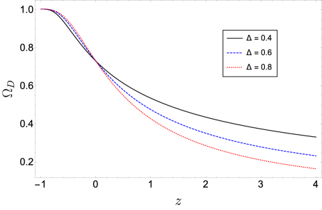
Figure 1: The evolution of $\Omega_{D}$ versus $z$ for different values of $\Delta$. We have set $\Omega_{k}=0.01$ and $\Omega_{D}^{0}=0.73$ as initial condition.

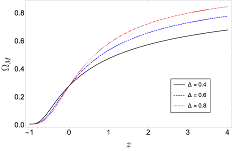
Figure 2: The evolution of $\Omega_{M}$ versus $z$ for different values of $\Delta$. We have set $\Omega_{k}=0.01$ and $\Omega_{D}^{0}=0.73$ as initial condition.

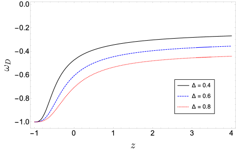
Figure 3: The evolution of $\omega_{D}$ versus $z$ for different values of $\Delta$. We have set $\Omega_{k}=0.01$ and $\Omega_{D}^{0}=0.73$ as initial condition.

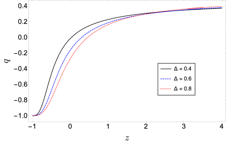
Figure 4: The evolution of $q$ versus $z$ for different values of $\Delta$. We have set $\Omega_{k}=0.01$ and $\Omega_{D}^{0}=0.73$ as initial condition.

To determine the behavior of BHDE, we solve this equation numerically. The evolution of $\Omega_{D}$ and $\Omega_{M}$ versus the redshift $z=\left(1-a\right)/a$ is plotted in Fig. 1 and Fig. 2 for different values of $\Delta$, respectively. From Fig. 1 it is evident that $\Omega_{D}$ increases monotonically going from early times to the far future. This indicates the evolution of the present model from an initial dark matter dominated phase toward a completely dark energy dominated epoch. The complementary behavior is exhibited by $\Omega_{M}$ (see Fig. 2).

The dynamics of EoS parameter is shown in Fig. 3. As we can see, $\omega_{D}$ lies in the quintessence regime ($-1<\omega_{D}<-1/3$) at present (i.e. $z=0$) and tends to the cosmological constant behavior $\omega_{D}=-1$ in the far future ($z\rightarrow-1$), regardless of $\Delta$. Specifically, for the current value of the EoS parameter the present model predicts $\omega_{D}^{0}\in[-0.72,-0.47]$ for the considered values of $\Delta$. Notice that this range is consistent with neither the recent observational constraints obtained from Planck+WP+Union 2.1 ($-1.26<\omega_{0}<-0.92$) and Planck+WP+BAO ($-1.38<\omega_{0}<-0.89$) data, nor with WMAP+eCMB+BAO+H0 ($-1.162<\omega_{0}<-0.983$) measurements Planck , thus requiring some proper amendment to this model.

For completeness, let us analyze the evolution of the deceleration parameter. By plugging Eqs. (18) and (19) into (14), this takes the form

$$q=\frac{1+\Omega_{k}-\left(1+\Delta\right)\Omega_{D}}{2+\left(\Delta-2\right)\Omega_{D}}\,.$$ (20)

The behavior of $q$ is plotted in Fig. 4 for different values of $\Delta$. As explained above, our model predicts the successive sequence of an early matter dominated era with a decelerated expansion ($q>0$), followed by a late time DE dominated epoch with an accelerated phase ($q<0$), In particular, the present framework is capable of explaining the observed accelerated phase of the Universe today ($z=0$), in contrast to the standard Holographic Dark Energy model. However, quantitatively speaking the redshift $z_{t}$ at which the transition from the decelerated to accelerated Universe occurs, i.e. $q(z_{t})=0$, lies within the interval $z_{t}\in[0.02,0.46]$ for the considered values of the model parameters. This range does not overlap with the observational constraint obtained via SNIa+BAO/CMB ($z_{t}=0.72\pm 0.05$) MamonEPJC2 , SNIa+CMB ($z_{t}=0.57\pm 0.07$) Alam and SNIa+CMB+LSS joint analysis ($z_{t}=0.61$) MamonMPA . Also, the value of the deceleration parameter for the current epoch is estimated as $q_{0}\in[-0.26,-0.01]$, to be compared with the experimental outcome $q_{0}=-0.64\pm 0.22$ from Union2 SNIa data WuHu . These results provide further evidence of the observational inconsistency of the non-interacting model.

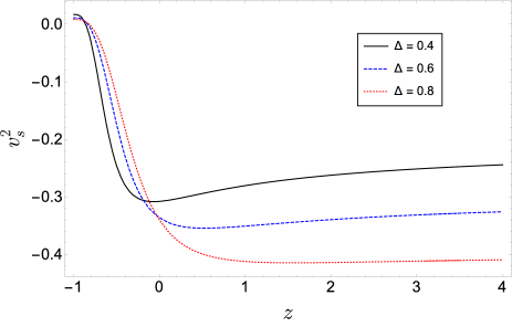
Figure 5: The evolution of $v_{s}^{2}$ versus $z$ for different values of $\Delta$. We have set $\Omega_{k}=0.01$ and $\Omega_{D}^{0}=0.73$ as initial condition.

From Eq. (17), we can finally derive the square of sound speed as

$$v_{s}^{2}=\frac{\left[\frac{3\Delta}{2}+\left(\frac{\Delta}{2}-1\right)\Omega_{k}\right]\left(\Omega_{D}-1\right)}{3\left[1-\left(1-\frac{\Delta}{2}\right)\Omega_{D}\right]^{2}}\,.$$ (21)

This is plotted as a function of the redshift $z$ in Fig. 5. Interestingly enough, we see that $v_{s}^{2}$ takes negative values at early and present times, while it tends to positive values in the far future. In other terms, the present model evolves towards a classically stable configuration. A similar result has been exhibited in hybrid for the case of BHDE with hybrid expansion law.

Figure 6 finally shows the behavior of the jerk parameter, which is given by the third derivative of the scale factor respect to the cosmic time, i.e. Rapetti

$$j\,=\,\frac{1}{aH^{3}}\frac{d^{3}a}{dt^{3}}=q\left(2q+1\right)+\left(1+z\right)\frac{dq}{dz}\,.$$ (22)

This quantity allows us to quantify departures from $\Lambda$CDM model, which is characterized by $j=1$. From Fig. 6, we find that $j>0$ for any redshift and approaches unity in the far future (i.e. $z\rightarrow-1$), where our model fits with $\Lambda$CDM. Also, we have $j_{0}\in[0.36,0.62]$ in the present epoch for the considered values of model parameters. Notice that deviations of $j_{0}$ from the $\Lambda$CDM value need attention as the real cause behind the cosmic acceleration is still unknown Bambabis .

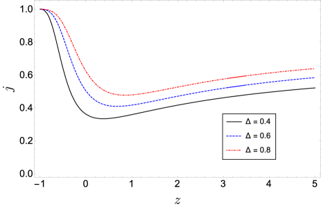
Figure 6: The evolution of $j$ versus $z$ for different values of $\Delta$. We have set $\Omega_{k}=0.01$ and $\Omega_{D}^{0}=0.73$ as initial condition.

III.2 Interacting model

We now extend the above analysis to the case where the interaction (12) between the dark sectors of the cosmos is taken into account. By repeating the same computations as above, we derive the following generalized expression for the EoS parameter

$$\omega_{D}=-\frac{3+\left(\frac{\Delta}{2}-1\right)\left(\Omega_{k}+3\right)+3b^{2}\left(1+r\right)}{3\left[1+\left(\frac{\Delta}{2}-1\right)\Omega_{D}\right]}\,.$$ (23)

Similarly, we get

$$\Omega_{D}^{\prime} = \frac{\Omega_{D}\,\Delta}{2}\,\frac{3+\Omega_{k}-3\Omega_{D}-3b^{2}\left(1+\Omega_{k}\right)}{1+\left(\frac{\Delta}{2}-1\right)\Omega_{D}}\,,$$ (24)

$$q = \frac{1+\Omega_{k}-\left(1+\Delta\right)\Omega_{D}-3b^{2}\left(1+\Omega_{k}\right)}{2+\left(\Delta-2\right)\Omega_{D}}\,,$$ (25)

$$v_{s}^{2} = \frac{\left[\frac{3\Delta}{2}+\left(\frac{\Delta}{2}-1\right)\Omega_{k}\right]\left(\Omega_{D}-1\right)}{3\left[1-\left(1-\frac{\Delta}{2}\right)\Omega_{D}\right]^{2}}$$ (26)

$$+\frac{b^{2}\left(1+\Omega_{k}\right)\left[1+\frac{\Delta}{2}+\frac{2}{\left(\Delta-2\right)\Omega_{D}}\right]}{\left[1-\left(1-\frac{\Delta}{2}\right)\Omega_{D}\right]^{2}}\,,$$

for the BHDE density, the deceleration parameter and the squared sound speed, respectively. It is straightforward to check that these relations correctly reduce to Eqs. (18), (19), (20) and (21) for $b^{2}=0$.

Fig. 7 shows the evolution of $\Omega_{D}$ versus $z$ for different values of $b^{2}$ (upper panel) and $\Delta$ (lower panel). On the other hand, in Fig. 8 we plot the behavior of $\Omega_{M}$. We can see that both these two densities exhibit the same profile as for the noninteracting case (see Fig. 1 and 2 for comparison). Remarkable differences can instead be highlighted from the analysis of the EoS parameter in Fig. 9. Indeed, in the present study the phantom line $\omega_{D}=-1$ is crossed in the far future. In particular, the higher the coupling, the more evident such a behavior (see upper panel of Fig. 9). This feature is peculiar to this model and has no correspondence in the noninteracting description (see Fig. 3). To check the observational consistency of the present model, let us compute the current value of the EoS parameter. From the lower panel of Fig. 9, we find $\omega_{D}^{0}\in[-0.96,-0.74]$, which is in agreement with constraints from Planck+WP+BAO and Planck+WP+Union 2.1 measurements (see the discussion above Eq. (20)).

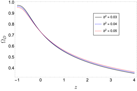
Figure 7: The evolution of $\Omega_{D}$ versus $z$ for different values of $b^{2}$ (upper panel) and $\Delta$ (lower panel). We have set $\Omega_{k}=0.01$ and $\Omega_{D}^{0}=0.73$ as initial condition. For the upper plot, we have considered $\Delta=0.4$, while for the lower one $b^{2}=0.01$.

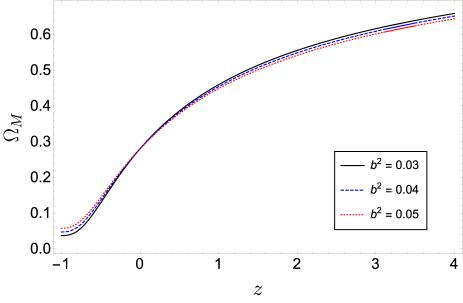
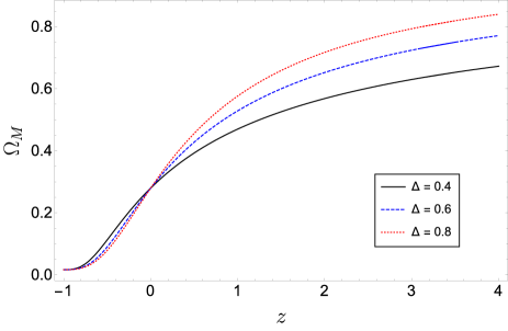
Figure 8: The evolution of $\Omega_{M}$ versus $z$ for different values of $b^{2}$ (upper panel) and $\Delta$ (lower panel). We have set $\Omega_{k}=0.01$ and $\Omega_{D}^{0}=0.73$ as initial condition. For the upper plot, we have considered $\Delta=0.4$, while for the lower one $b^{2}=0.01$.

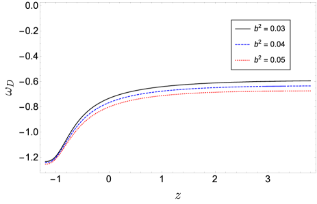
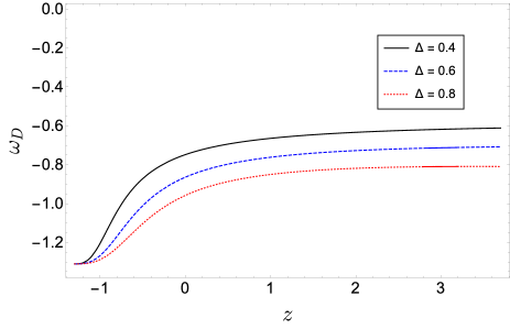
Figure 9: The evolution of $\omega_{D}$ versus $z$ for different values of $b^{2}$ (upper panel) and $\Delta$ (lower panel). We have set $\Omega_{k}=0.01$ and $\Omega_{D}^{0}=0.73$ as initial condition. For the upper plot, we have considered $\Delta=0.4$, while for the lower one $b^{2}=0.01$.

In Fig. 10 we show the evolution of the deceleration parameter $q$. We see that the interacting BHDE model still predicts a smooth transition of the Universe from an initial decelerated phase to a late-time accelerated expansion. However, the advantage of this framework over the non-interacting one is that the transition redshift is now estimated as $z_{t}\in[0.30,0.64]$, which is in good agreement with SNIa+CMB+LSS joint analysis. Also, the deceleration parameter for the current epoch is found to lie in the range $q_{0}\in[-0.33,-0.03]$ (see the lower panel in Fig. 10), the lower bound of which is closer to the experimental value exhibited in WuHu . Thus, the present model turns out to be favored by observations.

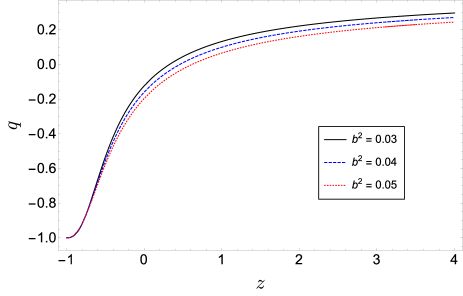
Figure 10: The evolution of $q$ versus $z$ for different values of $b^{2}$ (upper panel) and $\Delta$ (lower panel). We have set $\Omega_{k}=0.01$ and $\Omega_{D}^{0}=0.73$ as initial condition. For the upper plot, we have considered $\Delta=0.4$, while for the lower one $b^{2}=0.01$.

The behavior of the squared sound speed is plotted in Fig. 11. By comparison with Fig. 5, we see that $v_{s}^{2}$ is now always negative, which implies that interacting BHDE is unstable at classical level against small perturbations.

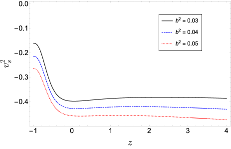
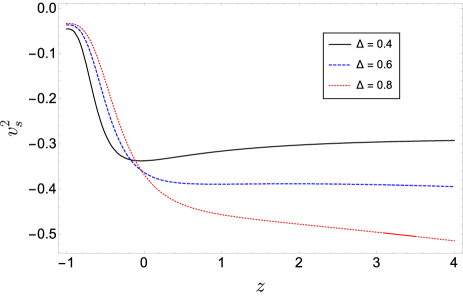
Figure 11: The evolution of $v_{s}^{2}$ versus $z$ for different values of $b^{2}$ (upper panel) and $\Delta$ (lower panel). We have set $\Omega_{k}=0.01$ and $\Omega_{D}^{0}=0.73$ as initial condition. For the upper plot, we have considered $\Delta=0.4$, while for the lower one $b^{2}=0.01$.

Figure 12 shows the jerk parameter (22) versus the redshift. As in the absence of interactions, we find that $j>0$ for any redshift, $j_{0}\in[0.35,0.64]$ (see the lower panel in Fig. 12) and $j\rightarrow 1$ in the far future (i.e. $z\rightarrow-1$), thus reproducing $\Lambda$CDM in this limit.

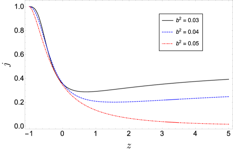
Figure 12: The evolution of $j$ versus $z$ for different values of $b^{2}$ (upper panel) and $\Delta$ (lower panel). We have set $\Omega_{k}=0.01$ and $\Omega_{D}^{0}=0.73$ as initial condition. For the upper plot, we have considered $\Delta=0.4$, while for the lower one $b^{2}=0.01$.

To further investigate the experimental relevance of the present model and constrain the free parameters $\Delta$, $b$ and $H_{0}$, let us consider the evolution of $H(z)$ from Eqs. (14) and (25) for fixed $\Omega_{k}=0.01$ and $\Omega_{D}^{0}=0.73$, and compare it with the data points obtained from the latest compilation of 57 Hubble’s parameter measurements in the range $0.07\leq z\leq 2.36$. Such points have been derived via Differential Age (31 points), BAO and other methods (the remaining 26 points) and are listed in Table 1 (see Koussour and references therein for more details on the data set).

Following Koussour , we use the statistical $R^{2}$-test to find the best fit values of model parameters. This is defined by

$$R^{2}\,=\,1-\frac{\sum_{i=1}^{57}\left[(H_{i})_{ob}-(H_{i})_{th}\right]^{2}}{\sum_{i=1}^{57}\left[(H_{i})_{ob}-(H_{i})_{mean}\right]^{2}}\,,$$ (27)

where $(H_{i})_{ob}$ and $(H_{i})_{th}$ are the observed and predicted values of Hubble’s parameter, respectively. Minimization of deviation of $R^{2}$ from unity gives the best-fit values $b=0.12$ and $\Delta=0.08$ at $95\%$ confidence level. We notice that the obtained estimation of Barrow parameter fits with the result $\Delta=0.094^{+0.093}_{-0.101}$ derived in Anagnostopoulos:2020ctz and is very close to the constraint $\Delta=0.075^{+0.001}_{-0.002}$ of Mathew , but it lies outside the intervals $0.005\leq\Delta\leq 0.008$ Luciano:2022pzg and $\Delta\lesssim 1.4\times 10^{-4}$ Barrow:2020kug found via baryogenesis and Big Bang Nucleosynthesis measurements, respectively. This discrepancy might be understood by assuming a HDE description of the Universe with a running Barrow entropy, as discussed in Dige .

From the fit in Fig. (13), we can also infer the current value of Hubble’s parameter predicted by the present model as $H_{0}=(63.3\pm 4.3)\,\mathrm{km\,s^{-1}\,Mpc^{-1}}$. This is consistent with the recent observation from Planck Collaboration $H_{0}=\left(67.27\pm 0.60\right)\mathrm{km\,s^{-1}\,Mpc^{-1}}$ Planck , but still deviates from the value $H_{0}=\left(74.03\pm 1.42\right)\mathrm{km\,s^{-1}\,Mpc^{-1}}$ based on the analysis of 2019 SH0ES collaboration SH0ES . More discussion on this point can be found in the concluding section.

$z$	$H(z)\,$	$\sigma_{H}$	$z\,$	$H(z)$	$\sigma_{H}$
0.070	69.0	19.6	0.4783	80	99
0.90	69	12	0.480	97	62
0.120	68.6	26.2	0.593	104	13
0.170	83	8	0.6797	92	8
0.1791	75	4	0.7812	105	12
0.1993	75	5	0.8754	125	17
0.200	72.9	29.6	0.880	90	40
0.270	77	14	0.900	117	23
0.280	88.8	36.6	1.037	154	20
0.3519	83	14	1.300	168	17
0.3802	83.0	13.5	1.363	160.0	33.6
0.400	95	17	1.430	177	18
0.4004	77.0	10.2	1.530	140	14
0.4247	87.1	11.2	1.750	202	40
0.4497	92.8	12.9	1.965	186.5	50.4
0.470	89	34

$z$	$H(z)\,$	$\sigma_{H}$	$z\,$	$H(z)$	$\sigma_{H}$
0.24	79.69	2.99	0.52	94.35	2.64
0.30	81.70	6.22	0.56	93.34	2.30
0.31	78.18	4.74	0.57	87.6	7.8
0.34	83.80	3.66	0.57	96.8	3.4
0.35	82.7	9.1	0.59	98.48	3.18
0.36	79.94	3.38	0.60	87.9	6.1
0.38	81.5	1.9	0.61	97.3	2.1
0.40	82.04	2.03	0.64	98.82	2.98
0.43	86.45	3.97	0.73	97.3	7.0
0.44	82.6	7.8	2.30	224.0	8.6
0.44	84.81	1.83	2.33	224	8
0.48	87.90	2.03	2.34	222.0	8.5
0.51	90.4	1.9	2.36	226.0	9.3

Table 1: 57 experimental points of $H(z)$: the first 31 have been obtained from the method of Differential Age, while the last 26 from BAO and other approaches ($H$ is expressed in $\mathrm{km\,s^{-1}\,Mpc^{-1}}$ and $\sigma_{H}$ represents the uncertainty for each data point).

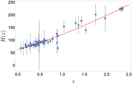
Figure 13: Best fit curve of Hubble’s parameter $H$ versus redshift $z$. Dots represent observed values, while the red curve is the theoretical fit.

IV Thermal stability of Barrow Holographic Dark Energy

Let us now study our model from the thermodynamic point of view. Toward this end, we follow the analysis of Abdollah ; Bhandari . In particular, we are going to investigate whether the thermal stability criteria are satisfied.

We start by defining the internal energy of the cosmic fluid (dark energy + dark matter) in the Universe as

$$E=V\left(\rho_{D}+\rho_{M}\right)\equiv V\rho_{T}\,,$$ (28)

where $V$ and $\rho_{T}$ are the volume and total energy density of the cosmic system, respectively. We can then write the thermodynamic relation Callen

$$TS=E+p_{D}V\,,$$ (29)

where $T$ denotes the temperature of the cosmic system and we have implicitly taken into account that DM is pressureless (i.e. $p_{M}=0$).

Inverting Eq. (29) respect to $E$ and using Eq. (28), we get

$$E=\frac{S\,T}{1+\omega_{T}}\,,$$ (30)

where $\omega_{T}\equiv p_{D}/\rho_{T}$ is the total EoS parameter of the cosmic fluid. The behavior of $\omega_{T}$ versus $z$ is plotted in Fig. 14 and Figs. 16-17 for noninteracting and interacting BHDE models, respectively. It can be seen that the evolution trajectories of this parameter are not considerably affected by either the curvature $\Omega_{k}$ or the interaction term $b^{2}$.

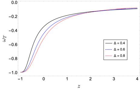
Figure 14: The evolution of $\omega_{T}$ versus $z$ for noninteracting BHDE model and different values of $\Delta$. We have set $\Omega_{D}^{0}=0.73$ as initial condition and $\Omega_{k}=0.01$ in the upper panel, while $\Omega_{k}=0$ in the lower one.

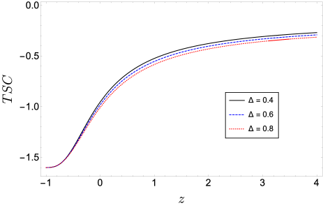
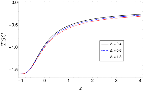
Figure 15: Thermal stability condition (TSC) for noninteracting BHDE. We have set $\Omega_{D}^{0}=0.73$ as initial condition and $\Omega_{k}=0.01$ in the upper panel, while $\Omega_{k}=0$ in the lower one.

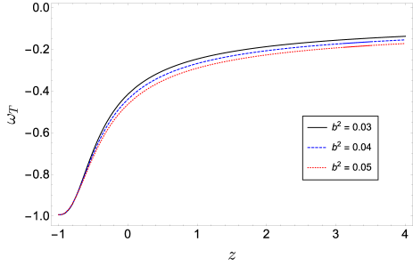
Figure 16: The evolution of $\omega_{T}$ versus $z$ for interacting BHDE model and different values of $b^{2}$. We have set $\Delta=0.4$ and $\Omega_{D}^{0}=0.73$ as initial condition. In the upper panel we have considered $\Omega_{k}=0.01$, while in the lower one $\Omega_{k}=0$.

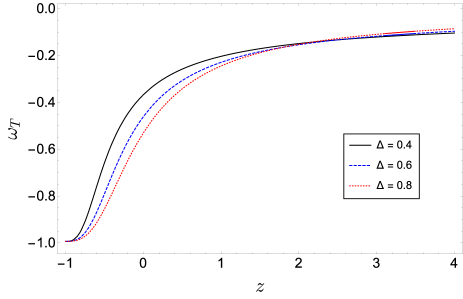
Figure 17: The evolution of $\omega_{T}$ versus $z$ for interacting BHDE model and different values of $\Delta$. We have set $b^{2}=0.01$ and $\Omega_{D}^{0}=0.73$ as initial condition. In the upper panel we have considered $\Omega_{k}=0.01$, while in the lower one $\Omega_{k}=0$.

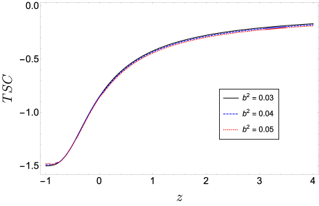
Figure 18: Thermal stability condition (TSC) for interacting BHDE and different values of $b^{2}$. We have set $\Delta=0.4$ and $\Omega_{D}^{0}=0.73$ as initial condition. In the upper panel we have considered $\Omega_{k}=0.01$, while in the lower one $\Omega_{k}=0$.

Let us now consider a reversible adiabatic expansion ($dS=0$). By using the first law of thermodyanmic combined with Eq. (30), we are led to Bhandari

$$E=E_{0}\left(\frac{1+\omega_{0}}{1+\omega_{T}}\right)\frac{T}{T_{0}}\,,$$ (31)

where $E_{0}$ and $T_{0}$ are the present values of the cosmic fluid energy and temperature, respectively, while $\omega_{0}$ is the present value of the total EoS parameter. Hence, comparison of Eqs. (30) and (31) gives

$$S=\frac{\left(1+\omega_{0}\right)E_{0}}{T_{0}}=const.$$ (32)

Additionally, using the heat capacities and the total energy-momentum conservation law, we obtain Barboza ; Bhandari

$$C_{v} = \left(\frac{\partial E}{\partial T}\right)_{V}=\frac{C_{p}\,d\log V}{\left(1+\omega_{T}\right)d\log V-d\log|\omega_{T}|}\,,$$ (33)

$$C_{p} = \left(\frac{\partial h}{\partial T}\right)_{p}=\frac{\left(1+\omega_{T}\right)E}{T}=\frac{\left(1+\omega_{0}\right)E_{0}}{T_{0}}=S\,,$$ (34)

where we have resorted to Eq. (31) in the third step of the second relation. Here, $C_{v}$ and $C_{p}$ are the heat capacities at constant volume and pressure, respectively, and

$$h=E+p\,V\,,$$ (35)

is the enthalpy of the cosmic fluid.

By combining Eqs. (33) and (34), one can show that

$$C_{p}=\left(1+\omega_{T}-\frac{d\log|\omega_{T}|}{d\log V}\right)C_{v}\,.$$ (36)

Let us also introduce the definitions of thermal expansivity, isothermal compressibility and adiabatic compressibility. They are given by

$$\alpha = \frac{1}{V}\left(\frac{\partial V}{\partial T}\right)_{p}\,,$$ (37)

$$\kappa_{T} = -\frac{1}{V}\left(\frac{\partial V}{\partial p}\right)_{T}\,,$$ (38)

$$\kappa_{S} = -\frac{1}{V}\left(\frac{\partial V}{\partial p}\right)_{S}\,,$$ (39)

respectively. By use of Eqs. (33)-(37), we then have Abdollah

$$\alpha=\frac{C_{v}}{V\rho_{T}\,\omega_{T}}\left(\omega_{T}-\frac{d\log|\omega_{T}|}{d\log V}\right).$$ (40)

Moreover, the following relations between the heat capacities $\kappa_{T}$ and $\kappa_{S}$ hold

$$\kappa_{T}=\frac{\alpha V}{C_{p}}\,,\qquad\kappa_{S}=\frac{\alpha VC_{v}}{C_{p}^{2}}\,,$$ (41)

$$\hskip 38.41121pt\frac{\kappa_{T}}{\kappa_{S}}=\frac{C_{p}}{C_{v}}\,.$$ (42)

We now analyze the thermal stability of the present system assuming that work is done due to the volume variation of the thermal system only. For stable equilibrium, it has been shown that the second order variation of the internal energy

$$\delta^{2}E=\delta T\,\delta S-\delta p\,\delta V\,,$$ (43)

must satisfy the condition $\delta^{2}E\geq 0$ Callen .

Notice that, by using Eqs. (33), (34), (38) and (39), we can equivalently cast Eq. (43) as

$$\delta^{2}E=V\,\kappa_{S}\,\delta p^{2}+\frac{T}{C_{p}}\delta S^{2}\,,$$ (44)

or

$$\delta^{2}E=\frac{1}{V\hskip 0.85358pt\kappa_{T}}\,\delta V^{2}+\frac{C_{v}}{T}\,\delta T^{2}\,.$$ (45)

Thus, for the stability of the system, the heat capacities and compressibilities should obey

$$C_{p},C_{v},\kappa_{S},\kappa_{T}\geq 0\,,$$ (46)

which, combined with Eqs. (41) and (42), leads to Abdollah

$$C_{p}\geq C_{v}\,,\qquad\kappa_{T}\geq\kappa_{S}\,.$$ (47)

From Eq. (34), it is straightforward to see that $C_{p}$ is constant and positive-definite. Moreover, Eqs. (36) and (40) imply that the constraints (47) and, thus, (46) are met only if the total EoS parameter $\omega_{T}$ obeys the Thermal Stability Condition (TSC)

$$\omega_{T}-\frac{d\log|\omega_{T}|}{d\log V}\geq 0\,.$$ (48)

In Fig. 15 and Fig. 18 the TSC has been plotted for the noninteracting and interacting cases, respectively. One can see that such criterion is not satisfied, indicating that the cosmic fluid is not thermodynamically stable in BHDE model.

V Conclusions and Outlook

We have analyzed the cosmic evolution of a nonflat FRW Universe filled by pressureless dark matter and BHDE. By considering the apparent horizon as IR cutoff, we have examined the evolutionary trajectories of various model parameters, such as the BHDE density parameter, the EoS parameter, the deceleration parameter, the jerk parameter and the squared sound speed. In the absence of interaction, we have found that $\omega_{D}$ never crosses the phantom line. Furthermore, the model successfully predicts the sequence of an early matter dominated era with a decelerated expansion, followed by a late time DE dominated epoch with an accelerated phase. Nevertheless, the values of the current EoS parameter, transition redshift and deceleration parameter are inconsistent with recent results in the literature (see Table 2).

On the other hand, assuming a mutual interaction between the dark sectors of the cosmos, we have obtained that BHDE enters the phantom regime in the future, with such a behavior being driven by the coupling $b^{2}$. The model still predicts the usual thermal history of the Universe and is consistent with observations for what concerns the values of the EoS parameter, transition redshift and deceleration parameter in the current epoch.

	Non-interacting model	Interacting model	Observational value
$\omega_{0}$	$[-0.72,-0.47]$	$[-0.96,-0.74]$	$[-1.38,-0.89]$  (Planck+WP+BAO)
$z_{t}$	$[0.02,0.46]$	$[0.30,0.64]$	$0.61$  (SNIa+CMB+LSS)
$q_{0}$	$[-0.26,-0.01]$	$[-0.33,-0.03]$	$[-0.86,-0.42]$  (Union2 SNIa)
$j_{0}$	$[0.36,0.62]$	$[0.35,0.64]$	$j=1$ ($\Lambda$CDM)
$H_{0}$	$-$	$(63.3\pm 4.3)\,\mathrm{km\,s^{-1}\,Mpc^{-1}}$	$\left(67.27\pm 0.60\right)\mathrm{km\,s^{-1}\,Mpc^{-1}}$ (Planck)

Table 2: Theoretical and observational values of EoS parameter, transition redshift, deceleration parameter, jerk parameter and Hubble parameter in the current epoch (for the jerk parameter we have considered the $\Lambda$CDM prediction as reference value).

Furthermore, for the interacting model we have studied the evolution of $H(z)$ and compared it with the data points obtained from the latest compilation of 57 Hubble’s parameter measurements from Differential Age, BAO and other approaches. By using the $R^{2}$-test, we have found the best fit of $H(z)$ for the model parameters $b=0.12$ and $\Delta=0.08$ (with $95\%$ confidence bounds). Also, the current value of Hubble parameter turns out to be $H_{0}=(63.3\pm 4.3)\,\mathrm{km\,s^{-1}\,Mpc^{-1}}$, which is consistent with the recent constraint from Planck Collaboration Planck , but is in tension with the observation from 2019 SH0ES Collaboration SH0ES . Along this line, it could be interesting to explore whether BHDE (or, more general, HDE based on deformed entropies) can play some role in solving the $H_{0}$ tension H0Tension . However, a detailed investigation of this issue would require the additional incorporation of CMB data and the development of a joint analysis. This aspect goes beyond the scope of our analysis and will be addressed in future works.

We have finally studied the thermal stability of our model by considering the heat capacities and compressibilities. We have shown that both the noninteracting and interacting frameworks suffer from the satisfaction of the Thermal Stability Condition (48). This result is in line with the achievement of Abdollah for the case of Tsallis Holographic Dark Energy and, more general, with the outcome of Barboza , where it has been found that DE fluids with a time-dependent EoS parameter are in conflict with the physical constraints imposed by thermodynamics.

Further aspects are still to be considered: first, one could investigate how the present study interfaces with the results of Mamon:2018flx , where it has been shown that some DE models, such as Chevallier-Polarski-Linder model, Generalized Chaplygin Gas and Modified Chaplygin Gas are thermodynamically stable for certain values of the model parameters. A potential path to explore is to see whether thermal stability for BHDE is achieved by considering different IR cutoffs and/or generalized interactions between the dark sectors of the cosmos. Of course, it is possible that even after such modifications the TSC is violated, indicating that BHDE may not be the answer to the question of the unknown DE.

Additionally, since our framework provides a preliminary attempt to study quantum gravity effects on the cosmic history of the Universe, it is worth analyzing to what extent it is consistent with predictions of more fundamental candidate theories of quantum gravity. Finally, we aim to examine in more detail the connection between BHDE and other models proposed to explain the origin of dark energy Yoo , and possibly fix more stringent constraints on the deformation parameter $\Delta$. These lines of research are under active investigation and are left for future projects.

- (1) C. Bambi and A. Dolgov, Introduction to Particle Cosmology: The Standard Model of Cosmology and its Open Problems. UNITEXT for Physics, Springer Berlin Heidelberg, 2015.
- (2) A. G. Riess et al. [Supernova Search Team], Astron. J. 116, 1009 (1998).
- (3) S. Perlmutter et al. [Supernova Cosmology Project], Astrophys. J. 517, 565 (1999).
- (4) D. N. Spergel et al. [WMAP], Astrophys. J. Suppl. 148, 175 (2003).
- (5) M. Tegmark et al. [SDSS], Phys. Rev. D 69, 103501 (2004).
- (6) P. A. R. Ade et al. [Planck], Astron. Astrophys. 571, A16 (2014).
- (7) A. G. Cohen, D. B. Kaplan and A. E. Nelson, Phys. Rev. Lett. 82, 4971 (1999).
- (8) P. Horava and D. Minic, Phys. Rev. Lett. 85, 1610 (2000).
- (9) S. D. Thomas, Phys. Rev. Lett. 89, 081301 (2002).
- (10) M. Li, Phys. Lett. B 603, 1 (2004).
- (11) S. D. H. Hsu, Phys. Lett. B 594, 13 (2004).
- (12) Q. G. Huang and M. Li, JCAP 08, 013 (2004).
- (13) B. Wang, C. Y. Lin and E. Abdalla, Phys. Lett. B 637, 357 (2006).
- (14) M. R. Setare, Phys. Lett. B 642, 421 (2006).
- (15) L.N. Granda, A. Oliveros, Phys. Lett. B 671275, 199 (2009).
- (16) A. Sheykhi, Phys. Rev. D 84, 107302 (2011).
- (17) K. Bamba, S. Capozziello, S. Nojiri and S. D. Odintsov, Astrophys. Space Sci. 342, 155 (2012).
- (18) S. Ghaffari, M. H. Dehghani and A. Sheykhi, Phys. Rev. D 89, 123009 (2014).
- (19) S. Wang, Y. Wang and M. Li, Phys. Rept. 696, 1 (2017).
- (20) H. Moradpour, A. H. Ziaie and M. Kord Zangeneh, Eur. Phys. J. C 80, 732 (2020).
- (21) X. Zhang and F. Q. Wu, Phys. Rev. D 72, 043524 (2005).
- (22) M. Li, X. D. Li, S. Wang and X. Zhang, JCAP 06, 036 (2009).
- (23) X. Zhang, Phys. Rev. D 79, 103509 (2009).
- (24) J. Lu, E. N. Saridakis, M. R. Setare and L. Xu, JCAP 03, 031 (2010).
- (25) J. D. Barrow, Phys. Lett. B 808, 135643 (2020).
- (26) F. K. Anagnostopoulos, S. Basilakos and E. N. Saridakis, Eur. Phys. J. C 80, 826 (2020).
- (27) G. Leon, J. Magaña, A. Hernández-Almada, M. A. García-Aspeitia, T. Verdugo and V. Motta, JCAP 12, 032 (2021).
- (28) J. D. Barrow, S. Basilakos and E. N. Saridakis, Phys. Lett. B 815, 136134 (2021).
- (29) K. Jusufi, M. Azreg-Aïnou, M. Jamil and E. N. Saridakis, Universe 8, 2 (2022).
- (30) M. P. Dabrowski and V. Salzano, Phys. Rev. D 102, 064047 (2020).
- (31) E. N. Saridakis and S. Basilakos, Eur. Phys. J. C 81, 644 (2021).
- (32) G. G. Luciano and E. N. Saridakis, Eur. Phys. J. C 82, 558 (2022).
- (33) S. Vagnozzi, R. Roy, Y. D. Tsai and L. Visinelli, [arXiv:2205.07787 [gr-qc]].
- (34) T. Padmanabhan, Phys. Rept. 406, 49-125 (2005).
- (35) E. N. Saridakis, Phys. Rev. D 102, 123525 (2020).
- (36) A. Sheykhi, Phys. Rev. D 103, 123503 (2021).
- (37) P. Adhikary, S. Das, S. Basilakos and E. N. Saridakis, Phys. Rev. D 104, 123519 (2021).
- (38) S. Nojiri, S. D. Odintsov and T. Paul, Phys. Lett. B 825 (2022), 136844.
- (39) G. G. Luciano and Y. Liu, [arXiv:2205.13458 [hep-th]].
- (40) S. Ghaffari, G. G. Luciano and S. Capozziello, [arXiv:2209.00903 [gr-qc]].
- (41) N. Radicella and D. Pavon, Gen. Rel. Grav. 44, 685 (2012).
- (42) J. P. Mimoso and D. Pavón, Phys. Rev. D 94, 103507 (2016).
- (43) H. Moradpour and N. Riazi, Int. J. Theor. Phys. 55, 268-277 (2016).
- (44) F. C. Santos, M. L. Bedran and V. Soares, Phys. Lett. B 636, 86 (2006).
- (45) E. M. Barboza, R. C. Nunes, E. M. C. Abreu and J. A. Neto, Phys. Rev. D 92, 083526 (2015).
- (46) P. Bhandari, S. Haldar and S. Chakraborty, Eur. Phys. J. C 77, 840 (2017).
- (47) M. Abdollahi Zadeh, A. Sheykhi and H. Moradpour, Gen. Rel. Grav. 51, 12 (2019).
- (48) M. Tavayef, A. Sheykhi, K. Bamba and H. Moradpour, Phys. Lett. B 781, 195 (2018).
- (49) E. N. Saridakis, K. Bamba, R. Myrzakulov and F. K. Anagnostopoulos, JCAP 12, 012 (2018).
- (50) S. Nojiri, S. D. Odintsov and E. N. Saridakis, Eur. Phys. J. C 79, 242 (2019)..
- (51) R. D’Agostino, Phys. Rev. D 99, 103524 (2019).
- (52) G. G. Luciano and J. Giné, Phys. Lett. B 833, 137352 (2022).
- (53) C. Tsallis and L. J. L. Cirto, Eur. Phys. J. C 73, 2487 (2013).
- (54) A. Sheykhi, Class. Quant. Grav. 27, 025007 (2010).
- (55) A. Sheykhi and M. Jamil, Phys. Lett. B 694, 284 (2011).
- (56) A. D. Chernin, D. I. Nagirner and S. V. Starikova, Astron. Astrophys. 399, 19 (2003).
- (57) G. F. R. Ellis and R. Maartens, Class. Quant. Grav. 21, 223 (2004).
- (58) B. Wang, Y. g. Gong and R. K. Su, Phys. Lett. B 605, 9 (2005).
- (59) E. Di Valentino, A. Melchiorri and J. Silk, Nature Astron. 4, 196 (2019).
- (60) S. Srivastava and U. K. Sharma, Int. J. Geom. Meth. Mod. Phys. 18, 2150014 (2021).
- (61) A. Sheykhi, Class. Quant. Grav. 27, 025007 (2010).
- (62) L. Granda and A. Oliveros, Phys. Lett. B 669, 275 (2008).
- (63) J. H. He and B. Wang, JCAP 06, 010 (2008.
- (64) D. Pavon and W. Zimdahl, Phys. Lett. B 628, 206 (2005).
- (65) H. Kim, Mon. Not. Roy. Astron. Soc. 364, 813 (2005).
- (66) Y. S. Myung, Phys. Lett. B 652, 223 (2007).
- (67) N. Aghanim et al. [Planck], Astron. Astrophys. 641, A6 (2020) [erratum: Astron. Astrophys. 652, C4 (2021)].
- (68) A. A. Mamon, K. Bamba and S. Das, Eur. Phys. J. C 77, 29 (2017).
- (69) U. Alam, V. Sahni and A. A. Starobinsky, JCAP 06, 008 (2004).
- (70) A. A. Mamon, Mod. Phys. Lett. A 33, no.10n11, 1850056 (2018).
- (71) Z. Li, P. Wu and H. Yu, Phys. Lett. B 695, 1 (2011).
- (72) M. Srivastava, M. Kumar and S. Srivastava, Grav. Cosmol. 28, 70 (2022).
- (73) D. Rapetti, S. W. Allen, M. A. Amin and R. D. Blandford, Mon. Not. Roy. Astron. Soc. 375, 1510 (2007).
- (74) A. Al Mamon and K. Bamba, Eur. Phys. J. C 78, 862 (2018).
- (75) M. Koussour, S. H. Shekh and M. Bennai, [arXiv:2203.08181 [gr-qc]].
- (76) N. K. P and T. K. Mathew, [arXiv:2112.07310 [gr-qc]].
- (77) S. Di Gennaro and Y. C. Ong, [arXiv:2205.09311 [gr-qc]].
- (78) A. G. Riess, S. Casertano, W. Yuan, L. M. Macri and D. Scolnic, Astrophys. J. 876, 85 (2019).
- (79) H. B. Callen, Thermodynamics and an Introduction to Thermostatistics, Wiley, New York (1985)
- (80) E. Di Valentino, L. A. Anchordoqui, O. Akarsu, Y. Ali-Haimoud, L. Amendola, N. Arendse, M. Asgari, M. Ballardini, S. Basilakos and E. Battistelli, et al. Astropart. Phys. 131, 102605 (2021).
- (81) A. A. Mamon, P. Bhandari and S. Chakraborty, Int. J. Geom. Meth. Mod. Phys. 16, 11 (2019).
- (82) J. Yoo and Y. Watanabe, Int. J. Mod. Phys. D 21, 1230002 (2012).