SeKron: A Decomposition Method Supporting Many Factorization Structures

Abstract

While convolutional neural networks (CNNs) have become the de facto standard for most image processing and computer vision applications, their deployment on edge devices remains challenging. Tensor decomposition methods provide a means of compressing CNNs to meet the wide range of device constraints by imposing certain factorization structures on their convolution tensors. However, being limited to the small set of factorization structures presented by state-of-the-art decomposition approaches can lead to sub-optimal performance. We propose SeKron, a novel tensor decomposition method that offers a wide variety of factorization structures, using sequences of Kronecker products. By recursively finding approximating Kronecker factors, we arrive at optimal decompositions for each of the factorization structures. We show that SeKron is a flexible decomposition that generalizes widely used methods, such as Tensor-Train (TT), Tensor-Ring (TR), Canonical Polyadic (CP) and Tucker decompositions. Crucially, we derive an efficient convolution projection algorithm shared by all SeKron structures, leading to seamless compression of CNN models. We validate SeKron for model compression on both high-level and low-level computer vision tasks and find that it outperforms state-of-the-art decomposition methods.

1 Introduction

Deep learning models have introduced new state-of-the-art solutions to both high-level computer vision problems (He et al. 2016; Ren et al. 2015), and low-level image processing tasks (Wang et al. 2018b; Schuler et al. 2015; Kokkinos & Lefkimmiatis 2018) through convolutional neural networks (CNNs). Such models are obtained at the expense of millions of training parameters that come along deep CNNs making them computationally intensive. As a result, many of these models are of limited use as they are challenging to deploy on resource-constrained edge devices. Compared with neural networks for high-level computer vision tasks (e.g., ResNet-50 (He et al. 2016)), models for low-level imaging problems such as single image super-resolution have much a higher computational complexity due to the larger feature map sizes. Moreover, they are typically infeasible to run on cloud computing servers. Thus, their deployment on edge devices is even more critical.

In recent years an increasing trend has begun in reducing the size of state-of-the-art CNN backbones through efficient architecture designs such as Xception (Chollet 2017), MobileNet (Howard et al. 2019), ShuffleNet (Zhang et al. 2018c), and EfficientNet (Tan & Le 2019), to name a few. On the other hand, there have been studies demonstrating significant redundancy in the parameters of large CNN models, implying that in theory the number of model parameters can be reduced while maintaining performance (Denil et al. 2013). These studies provide the basis for the development of many model compression techniques such as pruning (He et al. 2020), quantization (Hubara et al. 2017), knowledge distillation (Hinton et al. 2015), and tensor decomposition (Phan et al. 2020).

Tensor decomposition methods such as Tucker (Kim et al. 2016), Canonical Polyadic (CP) (Lebedev et al. 2015), Tensor-Train (TT) (Novikov et al. 2015) and Tensor-Ring (TR) (Wang et al. 2018a) rely on finding low-rank approximations of tensors under some imposed factorization structure as illustrated in Figure 1a. In practice, some structures are more suitable than others when decomposing tensors. Choosing from a limited set of factorization structures can lead to sub-optimal compressions as well as lengthy runtimes depending on the hardware. This limitation can be alleviated by reshaping tensors prior to their compression to improve performance as shown in (Garipov et al. 2016). However, this approach requires time-consuming development of customized convolution algorithms.

(a)

Tucker

CP

TR

TT

SeKron

(b)

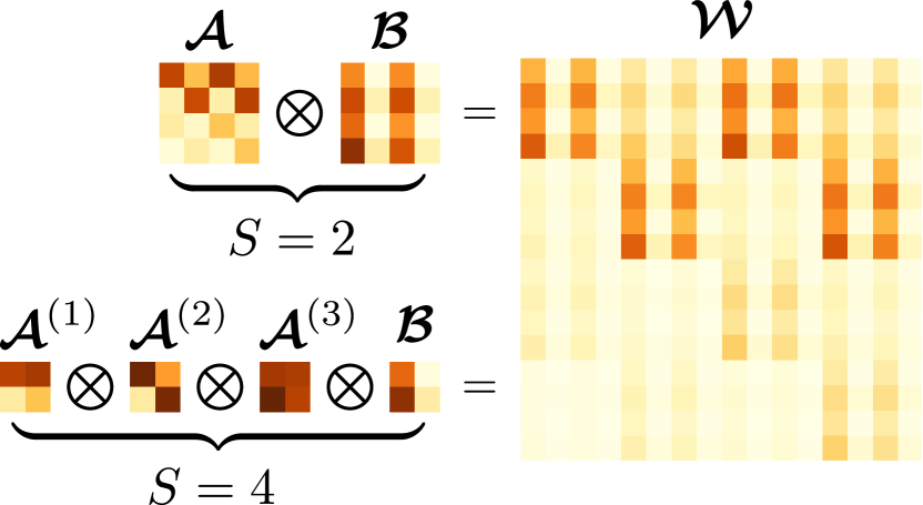
(a) SeKron with two sequence lengths

Figure 1: (a): Tensor network diagrams of various decomposition methods for a 4D convolution tensor $\tensorp{\bm{\mathcal{{W}}}}{}\in{\rm I\!R}^{F\times C\times K_{h}\times K_{w}}$. Unlike all other decomposition methods where $f,c,h,w$ index over fixed dimensions (i.e., dimensions of $\tensorp{\bm{\mathcal{{W}}}}{}$), SeKron is flexible in its factor dimensions, with ${\color[rgb]{1,0,0}f_{k}},{\color[rgb]{1,0,0}c_{k}},{\color[rgb]{1,0,0}h_{k}},{\color[rgb]{1,0,0}w_{k}},\forall k\in\{1,...,S\}$ indexing over variable dimension choices, as well as its sequence length $S$. Thus, it allows for a wide range of factorization structures to be achieved. (b): Example of a 16 $\times$ 16 tensor $\tensorp{\bm{\mathcal{{W}}}}{}$ that can be more efficiently represented using a sequence of four Kronecker factors (requiring 16 parameters) in contrast to using a sequence length of two (requiring 32 parameters).

We propose SeKron, a novel tensor decomposition method offering a wide range of factorization structures that share the same efficient convolution algorithm. Our method is inspired by approaches based on the Kronecker Product Decomposition (Thakker et al. 2019; Hameed et al. 2022). Unlike other decomposition methods, Kronecker Product Decomposition generalizes the product of smaller factors from vectors and matrices to a range of tensor shapes, thereby exploiting local redundancy between arbitrary slices of multi-dimensional weight tensors. SeKron represents tensors using sequences of Kronecker products to compress convolution tensors in CNNs. We show that using sequences of Kronecker products unlocks a wide range of factorization structures and generalizes other decomposition methods such as Tensor-Train (TT), Tensor-Ring (TR), Canonical Polyadic (CP) and Tucker, under the same framework. Sequences of Kronecker products also have the potential to exploit local redundancies using far fewer parameters as illustrated in the example in Figure 1b. By performing the convolution operation using each of the Kronecker factors independently, the number of parameters, computational intensity, and runtime are reduced, simultaneously. Leveraging the flexibility SeKron, we find efficient factorization structures that outperform existing decomposition methods on various image classification and low-level image processing super-resolution tasks. In summary, our contributions are:

• Introducing SeKron, a novel tensor decomposition method based on sequences of Kronecker products that allows for a wide range of factorization structures and generalizes other decomposition methods such as TT, TR, CP and Tucker.

• Providing a solution to the problem of finding the summation of sequences of Kronecker products between factor tensors that best approximates the original tensor.

• Deriving a single convolution algorithm shared by all factorization structures achievable by SeKron, utilized as compressed convolutional layers in CNNs.

• Improving the state-of-the-art of low-rank model compression on image classification (high-level vision) benchmarks such as ImageNet and CIFAR-10, as well as super-resolution (low-level vision) benchmarks such as Set4, Set14, B100 and Urban100.

2 Related Work on DNN Model Compression

Sparsification. Different components of DNNs, such as weights (Han et al. 2015b; a), convolutional filters (He et al. 2018; Luo et al. 2017) and feature maps (He et al. 2017; Zhuang et al. 2018) can be sparse. The sparsity can be enforced using sparsity-aware regularization (Liu et al. 2015; Zhou et al. 2016) or pruning techniques (Luo et al. 2017; Han et al. 2015b). Many pruning methods (Luo et al. 2017; Zhang et al. 2018b) aim for a high compression ratio and accuracy regardless of the structure of the sparsity. Thus, they often suffer from imbalanced workload caused by irregular memory access. Hence, several works aim at zeroing out structured groups of DNN components through more hardware friendly approaches (Wen et al. 2016).

Quantization. The computation and memory complexity of DNNs can be reduced by quantizing model parameters into lower bit-widths; wherein the majority of research works use fixed-bit quantization. For instance, the methods proposed in (Gysel et al. 2018; Louizos et al. 2018) use fixed 4 or 8-bit quantization. Model parameters have been quantized even further into ternary (Li et al. 2016; Zhu et al. 2016) and binary (Courbariaux et al. 2015; Rastegari et al. 2016; Courbariaux et al. 2016), representations. These methods often achieve low performance even with unquantized activations (Li et al. 2016). Mixed-precision approaches, however, achieve more competitive performance as shown in (Uhlich et al. 2019) where the bit-width for each layer is determined in an adaptive manner. Also, choosing a uniform (Jacob et al. 2018) or nonuniform (Han et al. 2015a; Tang et al. 2017; Zhang et al. 2018a) quantization interval has important effects on the compression rate and the acceleration.

Tensor Decomposition. Tensor decomposition approaches are based on factorizing weight tensors into smaller tensors to reduce model sizes (Yin et al. 2021). Singular value decomposition (SVD) applied on matrices as a 2-dimensional instance of tensor decomposition is used as one of the pioneering approaches to perform model compression (Jaderberg et al. 2014). Other classical high-dimensional tensor decomposition methods, such as Tucker (Tucker 1963) and CP decomposition (Harshman et al. 1970), are also adopted to perform model compression. However, using these methods often leads to significant accuracy drops (Kim et al. 2015; Lebedev et al. 2015; Phan et al. 2020). The idea of reshaping weights of fully-connected layers into high-dimensional tensors and representing them in TT format (Oseledets 2011) was extended to CNNs in (Garipov et al. 2016). For multidimensional tensors, TR decomposition (Wang et al. 2018a) has become a more popular option than TT (Wang et al. 2017). Subsequent filter basis decomposition works polished these approaches using a shared filter basis. They have been proposed for low-level computer vision tasks such as single image super-resolution in (Li et al. 2019). Kronecker factorization is another approach to replace the weight tensors within fully-connected and convolution layers (Zhou et al. 2015). The rank-1 Kronecker product representation limitation of this approach is alleviated in (Hameed et al. 2022). The compression rate in (Hameed et al. 2022) is determined by both the rank and factor dimensions. For a fixed rank, the maximum compression is achieved by selecting dimensions for each factor that are closest to the square root of the original tensors’ dimensions. This leads to representations with more parameters than those achieved using sequences of Kronecker products as shown in Fig. 1b.

There has been extensive research on tensor decomposition through characterizing global correlation of tensors (Zheng et al. 2021), extending CP to non-Gaussian data (Hong et al. 2020), employing augmented decomposition loss functions (Afshar et al. 2021), etc. for different applications. Our main focus in this paper is on the ones used for NN compression.

Other Methods NNs can also be compressed using Knowledge Distillation (KD) where a large pre-trained network known as teacher is used to train a smaller student network (Mirzadeh et al. 2020; Heo et al. 2019). Sharing weights in a more structured manner can be another model compression approach as FSNet (Yang et al. 2020) which shares filter weights across spatial locations or ShaResNet (Boulch 2018) which reuses convolutional mappings within the same scale level. Designing lightweight CNNs (Sandler et al. 2018; Iandola et al. 2016; Chollet 2017; Howard et al. 2019; Zhang et al. 2018c; Tan & Le 2019) is another direction orthogonal to the aforementioned approaches.

3 Method

In this section, we introduce SeKron and how it can be used to compress tensors in deep learning models. We start by providing background on the Kronecker Product Decomposition in Section 3.1. Then, we introduce our decomposition method in 3.2. In Section 3.3, we provide an algorithm for computing the convolution operation using each of the factors directly (avoiding reconstruction) at runtime. Finally, we discuss the computational complexity of the proposed method in Section 3.4.

3.1 Preliminaries

Convolutional layers prevalent in CNNs transform an input tensor $\tensorp{\bm{\mathcal{{X}}}}{}\in{\rm I\!R}^{C\times K_{h}\times K_{w}}$ using a weight tensor $\tensorp{\bm{\mathcal{{W}}}}{}\in{\rm I\!R}^{F\times C\times K_{h}\times K_{w}}$ via a multi-linear map given by

$$\tensorp{\bm{\mathcal{{Y}}}}{}_{f,x,y}=\sum_{i=1}^{K_{h}}\sum_{j=1}^{K_{w}}\sum_{c=1}^{C}\tensorp{\bm{\mathcal{{W}}}}{}_{f,c,i,j}\tensorp{\bm{\mathcal{{X}}}}{}_{c,i+x,j+y},$$ (1)

where $C$ and $F$ denote the number of input channels and output channels, respectively, and $K_{h}\times K_{w}$ denotes the spatial size of the weight (filter). Tensor decomposition seeks a compact approximation to replace $\tensorp{\bm{\mathcal{{W}}}}{}$, typically through finding lower-rank tensors using SVD.

One possible way of obtaining such a compact approximation comes from the fact that any tensor $\tensorp{\bm{\mathcal{{W}}}}{}\in{\rm I\!R}^{w_{1}\times\cdots\times w_{N}}$ can be written as sum of Kronecker products (Hameed et al. 2022). Let the Kronecker product between two matrices ${\mathbf{A}}\in{\rm I\!R}^{a_{1}\times a_{2}}$ and ${\mathbf{B}}\in{\rm I\!R}^{b_{1}\times b_{2}}$ be given by

$${\mathbf{A}}\otimes{\mathbf{B}}\triangleq\begin{bmatrix}A_{11}{\mathbf{B}}&\dots&A_{1a_{2}}{\mathbf{B}}\\ \vdots&\ddots&\vdots\\ A_{a_{1}1}{\mathbf{B}}&\dots&A_{a_{1}a_{2}}{\mathbf{B}}\end{bmatrix},$$ (2)

which can be extended to two multi-way tensors $\tensorp{\bm{\mathcal{{A}}}}{}\in{\rm I\!R}^{a_{1}\times\dots\times a_{N}}$ and $\tensorp{\bm{\mathcal{{B}}}}{}\in{\rm I\!R}^{b_{1}\times\dots\times b_{N}}$ as

$$(\tensorp{\bm{\mathcal{{A}}}}{}\otimes\tensorp{\bm{\mathcal{{B}}}}{})_{i_{1}\cdots i_{N}}\triangleq\tensorp{\bm{\mathcal{{A}}}}{}_{j_{1}\cdots j_{N}}\tensorp{\bm{\mathcal{{B}}}}{}_{k_{1}\cdots k_{N}},$$ (3)

where $j_{n}=\left\lfloor\frac{i_{n}}{b_{n}}\right\rfloor,\hskip 7.0ptk_{n}=i_{n}\hskip 1.0pt\text{mod}\hskip 1.0ptb_{n}$. Since $\tensorp{\bm{\mathcal{{W}}}}{}$ can be written as a sum of Kronecker products, i.e. $\tensorp{\bm{\mathcal{{W}}}}{}=\sum_{r=1}^{R}\tensorp{\bm{\mathcal{{A}}}}{}_{r}\otimes\tensorp{\bm{\mathcal{{B}}}}{}_{r},$ it can be approximated using a lower-rank representation by solving

$$\underset{\{\tensorp{\bm{\mathcal{{A}}}}{}_{r}\},\{\tensorp{\bm{\mathcal{{B}}}}{}_{r}\}}{\min}\left\|\tensorp{\bm{\mathcal{{W}}}}{}-\sum_{r=1}^{\widehat{R}}\tensorp{\bm{\mathcal{{A}}}}{}_{r}\otimes\tensorp{\bm{\mathcal{{B}}}}{}_{r}\right\|_{\mathrm{F}}^{2},$$ (4)

for $\widehat{R}$ sums of Kronecker products ($\widehat{R}\leq R$) using the SVD of a particular reshaping (unfolding) of $\tensorp{\bm{\mathcal{{W}}}}{}$, where $||\cdot||_{\mathrm{F}}$ denotes the Frobenius norm. Thus, the convolutional layer can be compressed by replacing $\tensorp{\bm{\mathcal{{W}}}}{}$ with $\sum_{r=1}^{\widehat{R}}\tensorp{\bm{\mathcal{{A}}}}{}_{r}\otimes\tensorp{\bm{\mathcal{{B}}}}{}_{r}$ in equation 1, where $\widehat{R}$ controls the compression rate.

3.2 SeKron Tensor Decomposition

The multi-way tensor representation in equation 3 can be extended to sequences of multi-way tensors

$$\left(\tensorp{\bm{\mathcal{{A}}}}{}^{(1)}\otimes\cdots\otimes\tensorp{\bm{\mathcal{{A}}}}{}^{(S)}\right)_{i_{1}\cdots i_{N}}\triangleq\tensorp{\bm{\mathcal{{A}}}}{}_{j_{1}^{(1)}\cdots j_{N}^{(1)}}^{(1)}\cdots\tensorp{\bm{\mathcal{{A}}}}{}_{j_{1}^{(S)}\cdots j_{N}^{(S)}}^{(S)},$$ (5)

where

$$j_{n}^{(k)}=\begin{cases}i_{n}-\sum_{t=1}^{k-2}j_{n}^{(t)}\prod_{l=t+1}^{S}a_{n}^{(l)}\text{mod}\,a_{n}^{(S)}\quad&k=S,\\ \left\lfloor\frac{i_{n}-\sum_{t=1}^{k-1}j_{n}^{(t)}\prod_{l=t+1}^{S}a_{n}^{(l)}}{\prod_{l=k+1}^{S}a_{n}^{(l)}}\right\rfloor\quad&\text{otherwise},\end{cases}$$ (6)

and $\tensorp{\bm{\mathcal{{A}}}}{}^{(k)}\in{\rm I\!R}^{a_{1}^{(k)}\times\dots\times a_{N}^{(k)}}$. Therefore, our decomposition method using sequences of Kronecker products i.e., SeKron, applied on a given tensor $\tensorp{\bm{\mathcal{{W}}}}{}\in{\rm I\!R}^{w_{1}\times\cdots\times w_{N}}$ involves finding a solution to

$$\underset{\{\tensorp{\bm{\mathcal{{A}}}}{}^{(k)}\}_{k=1}^{S}}{\min}\left\|\tensorp{\bm{\mathcal{{W}}}}{}-\sum_{r_{1}=1}^{R_{1}}\tensorp{\bm{\mathcal{{A}}}}{}_{r_{1}}^{(1)}\otimes\sum_{r_{2}=1}^{R_{2}}\tensorp{\bm{\mathcal{{A}}}}{}_{r_{1}r_{2}}^{(2)}\otimes\cdots\otimes\sum_{r_{S-1}=1}^{R_{S-1}}\tensorp{\bm{\mathcal{{A}}}}{}_{r_{1}\cdots r_{S-1}}^{(S-1)}\otimes\tensorp{\bm{\mathcal{{A}}}}{}_{r_{1}\cdots r_{S-1}}^{(S)}\right\|_{\mathrm{F}}^{2}.$$ (7)

Although this is a non-convex optimization problem, we provide a solution based on recursive application of SVD and demonstrate its quasi-optimality:

Theorem 1 (Tensor Decomposition using a Sequence of Kronecker Products).

Any tensor $\tensorp{\bm{\mathcal{{W}}}}{}$ $\in$ ${\rm I\!R}^{w_{1}\times\cdots\times w_{N}}$ can be represented by a sequence of Kronecker products between $S\in{\rm I\!N}$ factors:

$$\tensorp{\bm{\mathcal{{W}}}}{}=\sum_{r_{1}=1}^{R_{1}}\tensorp{\bm{\mathcal{{A}}}}{}_{r_{1}}^{(1)}\otimes\sum_{r_{2}=1}^{R_{2}}\tensorp{\bm{\mathcal{{A}}}}{}_{r_{1}r_{2}}^{(2)}\otimes\cdots\otimes\sum_{r_{S-1}=1}^{R_{S-1}}\tensorp{\bm{\mathcal{{A}}}}{}_{r_{1}\cdots r_{S-1}}^{(S-1)}\otimes\tensorp{\bm{\mathcal{{A}}}}{}_{r_{1}\cdots r_{S-1}}^{(S)},$$ (8)

where $R_{i}$ are ranks of intermediate matrices and $\tensorp{\bm{\mathcal{{A}}}}{}^{(k)}\in{\rm I\!R}^{a_{1}^{(k)}\times\cdots\times a_{N}^{(k)}}$.

Proof.

See Appendix ∎

Our approach to solving equation 7 involves finding two approximating Kronecker factors that minimize the reconstruction error with respect to the original tensor, then recursively applying this procedure on the latter factor found. More precisely, we define intermediate tensors

$$\tensorp{\bm{\mathcal{{B}}}}{}_{r_{1}\cdots r_{k}}^{(k)}\triangleq\sum_{r_{k+1}=1}^{R_{k+1}}\tensorp{\bm{\mathcal{{A}}}}{}_{r_{1}\cdots r_{k+1}}^{(k+1)}\otimes\sum_{r_{k+2}=1}^{R_{k+2}}\tensorp{\bm{\mathcal{{A}}}}{}_{r_{1}\cdots r_{k+2}}^{(k+2)}\otimes\cdots\otimes\sum_{r_{S-1}=1}^{R_{S-1}}\tensorp{\bm{\mathcal{{A}}}}{}_{r_{1}\cdots r_{S-1}}^{(S-1)}\otimes\tensorp{\bm{\mathcal{{A}}}}{}_{r_{1}\cdots r_{S-1}}^{(S)},$$ (9)

allowing us to re-write the reconstruction error in equation 7, for the $k^{th}$ iteration, as

$$\underset{\begin{subarray}{c}\{\tensorp{\bm{\mathcal{{A}}}}{}_{r_{1}\cdots r_{k}}^{(k)},\;\tensorp{\bm{\mathcal{{B}}}}{}_{r_{1}\cdots r_{k}}^{(k)}\}\\ r_{j}=1,\cdots R_{j},\;j=1,\dots,k\end{subarray}}{\min}\left\|\tensorp{\bm{\mathcal{{W}}}}{}_{r_{1}\cdots r_{k-1}}^{(k)}-\sum_{r_{k}=1}^{R_{k}}\tensorp{\bm{\mathcal{{A}}}}{}_{r_{1}\cdots r_{k}}^{(k)}\otimes\tensorp{\bm{\mathcal{{B}}}}{}^{(k)}_{r_{1}\cdots r_{k}}\right\|_{\mathrm{F}}^{2}.$$ (10)

In the first iteration, the tensor being decomposed is the original tensor (i.e., $\tensorp{\bm{\mathcal{{W}}}}{}^{(1)}\leftarrow\tensorp{\bm{\mathcal{{W}}}}{}$). Whereas in subsequent iterations, intermediate tensors are decomposed. At each iteration, we can convert the problem in equation 10 to the low-rank matrix approximation problem

$$\underset{\begin{subarray}{c}\{{\mathbf{a}}_{r_{1}\cdots r_{k}}^{(k)},\;{\mathbf{b}}_{r_{1}\cdots r_{k}}^{(k)}\}\\ r_{j}=1,\cdots R_{j},\;j=1,\dots,k\end{subarray}}{\min}\left\|{\mathbf{W}}_{r_{1}\cdots r_{k-1}}^{(k)}-\sum_{r_{k}=1}^{R_{k}}{\mathbf{a}}_{r_{1}\cdots r_{k}}^{(k)}{\mathbf{b}}^{(k)\top}_{r_{1}\cdots r_{k}}\right\|_{\mathrm{F}}^{2},$$ (11)

through reshaping, such that the overall sum of squares is preserved between equation 10 and equation 11. The problem in equation 11 can be readily solved, as it has a well known solution using SVD. The reshaping operations that facilitate this transformation are

$${\mathbf{W}}_{r_{1}\cdots r_{k-1}}^{(k)}=\textsc{Mat}(\textsc{Unfold}(\tensorp{\bm{\mathcal{{W}}}}{}_{r_{1}\cdots r_{k-1}}^{(k)},{\mathbf{d}}_{\tensorp{\bm{\mathcal{{B}}}}{}_{r_{1}\cdots r_{k}}^{(k)}})),$$ (12)

$${\mathbf{a}}_{r_{1}\cdots r_{k}}^{(k)}=\textsc{Unfold}(\tensorp{\bm{\mathcal{{A}}}}{}_{r_{1}\cdots r_{k}}^{(k)},{\mathbf{d}}_{\tensorp{\bm{\mathcal{{I}}}}{}_{\tensorp{\bm{\mathcal{{A}}}}{}_{r_{1}\cdots r_{k}}^{(k)}}}),\;\;{\mathbf{b}}_{r_{1}\cdots r_{k}}^{(k)}=\textsc{Vec}(\tensorp{\bm{\mathcal{{B}}}}{}_{r_{1}\cdots r_{k}}^{(k)}),\vspace{-2mm}$$ (13)

where Unfold reshapes tensor $\tensorp{\bm{\mathcal{{W}}}}{}_{r_{1}\cdots r_{k-1}}^{(k)}$ by extracting multidimensional patches of shape ${\mathbf{d}}_{\tensorp{\bm{\mathcal{{B}}}}{}_{r_{1},\dots r_{k}}^{(k)}}$ from tensor $\tensorp{\bm{\mathcal{{W}}}}{}_{r_{1}\cdots r_{k-1}}^{(k)}$ in any order, ${\mathbf{d}}_{\tensorp{\bm{\mathcal{{B}}}}{}}$ denotes a vector describing the shape of a tensor $\tensorp{\bm{\mathcal{{B}}}}{}$, $\textsc{Vec}:{\rm I\!R}^{d_{1}\times\cdots\times d_{N}}\to{\rm I\!R}^{d_{1}\cdots d_{N}}$ flattens a tensor to a 1D vector, $\textsc{Mat}:{\rm I\!R}^{d_{1}\times\cdots\times d_{N}}\to{\rm I\!R}^{d_{1}\cdots d_{N}}$ reshapes a tensor to a matrix and $\tensorp{\bm{\mathcal{{I}}}}{}_{\tensorp{\bm{\mathcal{{A}}}}{}}$ denotes an identity tensor which has the same number of dimensions as tensor $\tensorp{\bm{\mathcal{{A}}}}{}$ with each dimension set to one.

Input: $\text{Input tensor}\,\tensorp{\bm{\mathcal{{W}}}}{}\in{\rm I\!R}^{w_{1}\times\cdots\times w_{N}}\;\;\text{Kronecker factor shapes}\ \{d^{(i)}\}_{i=1}^{S}$

Output: $\text{Kronecker factors}\;\{\tensorp{\bm{\mathcal{{A}}}}{}\}_{i=1}^{S}$

for $i\leftarrow 1,2,\dots,S-1$ do

       ${\mathbf{d}}^{(a)}\leftarrow{\mathbf{d}}^{(i)}$

       ${\mathbf{d}}^{(b)}\leftarrow\prod_{k=i+1}^{S}{\mathbf{d}}^{(k)}$

       ${\mathbf{W}}\leftarrow\textsc{Unfold}(\tensorp{\bm{\mathcal{{W}}}}{},\,\text{shape}={\mathbf{d}}^{(b)})$ // ${\rm I\!R}^{B\times L\times\prod_{k=1}^{N}d_{k}^{(b)}}$

       ${\mathbf{U}},{\mathbf{s}},{\mathbf{V}}\leftarrow\textsc{SVD}({\mathbf{W}})$ // ${\mathbf{U}}\in{\rm I\!R}^{B\times L\times R}$ where $R=\text{min}(L,\prod_{k=1}^{N}d_{k}^{(b)})$

       $\tensorp{\bm{\mathcal{{A}}}}{}^{(i)}\leftarrow\textsc{Stack}((\textsc{Reshape}({\mathbf{U}}_{b,:,r},\,\text{shape}={\mathbf{d^{(a)}}})\,|\,b=1,2,\dots B,\;r=1,2,\dots R))$

       $\tensorp{\bm{\mathcal{{B}}}}{}^{(i)}\leftarrow\textsc{Stack}((\textsc{Reshape}(s_{k}{\mathbf{V}}^{\top}_{b,:,r},\,\text{shape}={\mathbf{d^{(b)}}})\,|\,b=1,2,\dots B,\;r=1,2,\dots R))$

       $\tensorp{\bm{\mathcal{{W}}}}{}\leftarrow\tensorp{\bm{\mathcal{{B}}}}{}^{(i)}$

      

end for

$\tensorp{\bm{\mathcal{{A}}}}{}^{(S)}\leftarrow\tensorp{\bm{\mathcal{{B}}}}{}^{S-1}$

return $\{\tensorp{\bm{\mathcal{{A}}}}{}\}_{i=1}^{S}$

Algorithm 1 SeKron Tensor Decomposition

Once each $\tensorp{\bm{\mathcal{{B}}}}{}_{r_{1}\cdots r_{k}}^{(k)}$ is obtained by solving equation 11 (and using the inverse of the Vec operation in equation 13), we proceed recursively by setting $\tensorp{\bm{\mathcal{{W}}}}{}_{r_{1}\cdots r_{k}}^{(k+1)}\leftarrow\tensorp{\bm{\mathcal{{B}}}}{}_{r_{1}\cdots r_{k}}^{(k)}$ and solving the $k+1^{th}$ iteration of equation equation 11. In other words, at the $k^{th}$ iteration, we find Kronecker factors $\tensorp{\bm{\mathcal{{A}}}}{}^{(k)}$ and $\tensorp{\bm{\mathcal{{B}}}}{}^{(k)}$, where the latter is used in the following iteration. Except in the final iteration (i.e., $k=S-1$), where the intermediate tensor $\tensorp{\bm{\mathcal{{B}}}}{}^{(k)}$ is the solution to the last Kronecker factor $\tensorp{\bm{\mathcal{{A}}}}{}^{(S)}$. Algorithm 1 presents this procedure, where for clarity, the recursive steps are unfolded in a for-loop.

By virtue of the connectivity between all of the Kronecker factors as illustrated in Figure 1a, SeKron generalizes many other decomposition methods. This result is formalized in the following theorem:

Theorem 2 (Generality of SeKron).

The CP, Tucker, TT and TR decompositions of a given tensor $\tensorp{\bm{\mathcal{{W}}}}{}\in{\rm I\!R}^{w_{1}\times\cdots\times w_{N}}$ are special cases of its SeKron decomposition.

Proof.

See Appendix. ∎

3.3 Convolution with SeKron Structures

In this section, we provide an efficient algorithm for performing a convolution operation using a tensor represented by a sequence of Kronecker factors. Assuming $\tensorp{\bm{\mathcal{{W}}}}{}$ is approximated as a sequence of Kronecker products using SeKron, i.e., $\tensorp{\bm{\mathcal{{W}}}}{}\approx\widehat{\tensorp{\bm{\mathcal{{W}}}}{}}$ and

$$\widehat{\tensorp{\bm{\mathcal{{W}}}}{}}=\sum_{r_{1}=1}^{\widehat{R}_{1}}\tensorp{\bm{\mathcal{{A}}}}{}_{r_{1}}^{(1)}\otimes\sum_{r_{2}=1}^{\widehat{R}_{2}}\tensorp{\bm{\mathcal{{A}}}}{}_{r_{1}r_{2}}^{(2)}\otimes\dots\sum_{r_{S-1}=1}^{\widehat{R}_{S-1}}\tensorp{\bm{\mathcal{{A}}}}{}_{r_{1}\cdots r_{S-1}}^{(S-1)}\otimes\tensorp{\bm{\mathcal{{A}}}}{}_{r_{1}\cdots r_{S-1}}^{(S)},$$ (14)

the convolution operation in equation 1 can be re-written as

$$\tensorp{\bm{\mathcal{{Y}}}}{}_{fxy}=\sum_{\begin{subarray}{c}i,j,c=1\end{subarray}}^{K_{h},K_{w},C}\Bigg{(}\sum_{r_{1}=1}^{\widehat{R}_{1}}\tensorp{\bm{\mathcal{{A}}}}{}_{r_{1}}^{(1)}\otimes\cdots\otimes\sum_{r_{S-1}=1}^{\widehat{R}_{S-1}}\tensorp{\bm{\mathcal{{A}}}}{}_{r_{1}\cdots r_{S-1}}^{(S-1)}\otimes\tensorp{\bm{\mathcal{{A}}}}{}_{r_{1}\cdots r_{S-1}}^{(S)}\Bigg{)}_{fcij}\tensorp{\bm{\mathcal{{X}}}}{}_{c,i+x,j+y}.$$ (15)

Due to the factorization structure of tensor $\widehat{\tensorp{\bm{\mathcal{{W}}}}{}}$, the projection in equation 15 can be carried out without its explicit reconstruction. Instead, the projection can be performed using each of the Kronecker factors independently. This property is essential to performing efficient convolution operations using SeKron factorizations, and leads to a reduction in both memory and FLOPs at runtime. In practice, this amounts to replacing one large convolution operation (i.e., one with a large convolution tensor) with a sequence of smaller grouped 3D convolutions, as summarized in Algorithm 2.

The ability to avoid reconstruction at runtime when performing a convolution using any SeKron factorization is the result of the following Theorem:

Theorem 3 (Linear Mappings with Sequences of Kronecker Products).

Any linear mapping using a given tensor $\tensorp{\bm{\mathcal{{W}}}}{}$ can be written directly in terms of its Kronecker factors $\tensorp{\bm{\mathcal{{A}}}}{}_{r_{1}\cdots r_{k}j_{1}^{(k)}\cdots j_{N}^{(k)}}^{(k)}\in{\rm I\!R}^{a_{1}^{(k)}\times\cdots\times a_{N}^{(k)}}$. That is:

$$\tensorp{\bm{\mathcal{{W}}}}{}_{i_{1}\cdots i_{N}}\tensorp{\bm{\mathcal{{X}}}}{}_{i_{1}+z_{1},\cdots,i_{N}+z_{N}}=\tensorp{\bm{\mathcal{{A}}}}{}_{r_{1}j_{1}^{(1)}\cdots j_{N}^{(1)}}^{(1)}\cdots\tensorp{\bm{\mathcal{{A}}}}{}_{r_{1}\cdots r_{S-1}j_{1}^{(S)}\cdots j_{N}^{(S)}}^{(S)}\tensorp{\bm{\mathcal{{X}}}}{}_{f({\mathbf{j}}_{1})+z_{1},\cdots,f({\mathbf{j}}_{N})+z_{N}}$$ (16)

where $j_{n}^{(k)}$ terms index Kronecker factors as in equation 6, and $f({\mathbf{j}}_{n})=\sum_{k=1}^{S}j_{n}^{(k)}\prod_{l=k+1}^{S}a_{n}^{(l)}$

Proof.

See Appendix ∎

Input: $\{\tensorp{\bm{\mathcal{{A}}}}{}^{(i)}\}_{i=1}^{S},\tensorp{\bm{\mathcal{{A}}}}{}^{(i)}\in{\rm I\!R}^{r_{i}\times f_{i}\times c_{i}\times Kh_{i}\times Kw_{i}}\quad\tensorp{\bm{\mathcal{{X}}}}{}\in{\rm I\!R}^{N\times C\times H\times W}$

Output: $\tensorp{\bm{\mathcal{{X}}}}{}\in{\rm I\!R}^{N\times\prod_{k=1}^{S}f_{k}\times H\times W}$

for $i\leftarrow S,S-1,\dots,1$ do

       if $i==S$ then

             $\tensorp{\bm{\mathcal{{X}}}}{}\leftarrow\textsc{Conv3d}(\textsc{Unsqueeze}(\tensorp{\bm{\mathcal{{X}}}}{},1),\textsc{Unsqueeze}(\tensorp{\bm{\mathcal{{A}}}}{}^{(i)},1)$

             /* ${\rm I\!R}^{N\times\prod_{k=i+1}^{S}f_{k}\times r_{i}f_{i}\times\prod_{k=1}^{i-1}c_{k}\times H\times W}\to{\rm I\!R}^{N\times\prod_{k=i}^{S}f_{k}\times r_{i-1}\times\prod_{k=1}^{i-1}c_{k}\times H\times W}$ */

             $\tensorp{\bm{\mathcal{{X}}}}{}\leftarrow\textsc{Reshape}_{1}(\tensorp{\bm{\mathcal{{X}}}}{})$

      else

             $\tensorp{\bm{\mathcal{{X}}}}{}\leftarrow\textsc{Conv3d}(\tensorp{\bm{\mathcal{{X}}}}{},\tensorp{\bm{\mathcal{{A}}}}{}^{(i)},\text{groups}=ri)$

             /* ${\rm I\!R}^{N\times\prod_{k=i+1}^{S}f_{k}\times r_{i}f_{i}\times\prod_{k=1}^{i-1}c_{k}\times H\times W}\to{\rm I\!R}^{N\times\prod_{k=i}^{S}f_{k}\times r_{i}\times\prod_{k=1}^{i-1}c_{k}\times H\times W}$ */

             $\tensorp{\bm{\mathcal{{X}}}}{}\leftarrow\textsc{Reshape}_{2}(\tensorp{\bm{\mathcal{{X}}}}{})$

       end if

      

end for

return $\tensorp{\bm{\mathcal{{X}}}}{}$

Algorithm 2 Convolution operation using a sequence of Kronecker factors

Using equation 16, we re-write the projection in equation 15 directly in terms of Kronecker factors

$$\tensorp{\bm{\mathcal{{Y}}}}{}_{fxy}=\sum_{\begin{subarray}{c}{\mathbf{i}},{\mathbf{j}},{\mathbf{c}},r_{1}\end{subarray}}\tensorp{\bm{\mathcal{{A}}}}{}_{r_{1}f_{1}c_{1}i_{1}j_{1}}^{(1)}\sum_{r_{2}}\tensorp{\bm{\mathcal{{A}}}}{}_{r_{1},r_{2},f_{2},c_{2},i_{2},j_{2}}^{(2)}\cdots\\ \sum_{r_{S-1}}\tensorp{\bm{\mathcal{{A}}}}{}_{r_{1}\cdots r_{S-1}f_{N-1}c_{N-1}i_{N-1}j_{N-1}}^{(S-1)}\tensorp{\bm{\mathcal{{A}}}}{}_{r_{1}\cdots r_{S-1}f_{N}c_{N}i_{N}j_{N}}^{(S)}\tensorp{\bm{\mathcal{{X}}}}{}_{f({\mathbf{c}}),f({\mathbf{i}})+x,f({\mathbf{j}})+y},$$ (17)

where ${\mathbf{i}}=(i_{1},i_{2},\dots,i_{N}),\;{\mathbf{j}}=(j_{1},j_{2},\dots,j_{N}),\;{\mathbf{c}}=(c_{1},c_{2},\dots,c_{N})$ denote vectors containing indices $i_{k},j_{k},c_{k}$ that enumerate over positions in tensors $\tensorp{\bm{\mathcal{{A}}}}{}^{(k)}$. Finally, exchanging the order of summation separates the convolution as follows:

$$\tensorp{\bm{\mathcal{{Y}}}}{}_{fxy}=\sum_{i_{1},j_{1},c_{1},r_{1}}\tensorp{\bm{\mathcal{{A}}}}{}_{r_{1}f_{1}c_{1}i_{1}j_{1}}^{(1)}\cdots\sum_{i_{N},j_{N},c_{N}}\tensorp{\bm{\mathcal{{A}}}}{}_{r_{1}\cdots r_{S-1}f_{N}c_{N}i_{N}j_{N}}^{(S)}\tensorp{\bm{\mathcal{{X}}}}{}_{f({\mathbf{c}}),f({\mathbf{i}})+x,f({\mathbf{j}})+y}.$$ (18)

Overall, the projection in equation 18 can be carried out efficiently using a sequence of grouped 3D convolutions with intermediate reshaping operations as described in Algorithm 2. Refer to Appendix for discussions on universal approximation properties of NN with weights represented using SeKron.

3.4 Computational Complexity

In order to decompose a given tensor using our method, the sequence length and the Kronecker factor shapes must be specified. Different selections will lead to different FLOPs, parameters, and latency. Specifically, for the decomposition given by equation 14 for $\widehat{\tensorp{\bm{\mathcal{{W}}}}{}}\in{\rm I\!R}^{f\times c\times h\times w}$ using factors $\tensorp{\bm{\mathcal{{A}}}}{}_{r_{1}\cdots r_{i}}^{(i)}\in{\rm I\!R}^{f_{i}\times c_{i}\times h_{i}\times w_{i}}$, the compression ratio (CR) and FLOPs reduction ratio (FR) are given by

$$\text{CR}=\frac{\prod_{i=1}^{S}f_{i}c_{i}h_{i}w_{i}}{\sum_{i=1}^{S}\prod_{k=1}^{i}\widehat{R}_{k}f_{i}c_{i}h_{i}w_{i}},\quad\text{FR}=\frac{\prod_{i=1}^{S}f_{i}c_{i}h_{i}w_{i}}{\sum_{i=1}^{S}\left(\prod_{k=i}^{S}F_{k}\right)\left(\prod_{k=1}^{i}\widehat{R}_{k}\right)\left(\prod_{k=1}^{i}c_{k}\right)h_{i}w_{i}}.\vspace{-1mm}$$ (19)

Applying SeKron to compress DNN models requires a selection strategy for sequence lengths and factor shapes for each layer in a network. We adopt a simple approach that involves selecting configurations that best match a desired CR while also having a lower latency than the original layer being compressed, as FR may not be a good indicator of runtime speedup in practice.

4 Experimental Results

To demonstrate the effectiveness of SeKron for model compression, we evaluate different CNN models on both high-level and low-level computer vision tasks. For image classification tasks, we evaluate WideResNet16 (Zagoruyko & Komodakis 2016) and ResNet50 (He et al. 2016) models on CIFAR-10 (Krizhevsky 2009) and ImageNet (Krizhevsky et al. 2012), respectively. For super-resolution task, we evaluate EDSR-8-128 and SRResNet16 trained on DIV2k(Agustsson & Timofte 2017). Lastly, we discuss the latency of our proposed decomposition method.

4.1 Image Classification Experiments

First, we evaluate SeKron to compress WideResNet16-8 (Zagoruyko & Komodakis 2016) for image classification on CIFAR-10. We evaluate our method against a range of decomposition and pruning approaches at various compression rates. Namely, PCA (Zhang et al. 2016) which imposes that filter responses lie approximately on a low-rank subspace; SVD-Energy (Alvarez & Salzmann 2017) which imposes a low-rank regularization into the training procedure; L-Rank (learned rank selection) (Idelbayev & Carreira-Perpinan 2020) which jointly optimizes over matrix elements and ranks; ALDS (Liebenwein et al. 2021) which provides a global compression framework that finds optimal layer-wise compressions that lead to an overall desired global compression rate; TR (Wang et al. 2018a); TT (Novikov et al. 2015) as well as two recent pruning approaches FT (Li et al. 2017) and PFP (Liebenwein et al. 2020). We note that since ALDS and L-Rank are rank selection frameworks, they can be used on top of other decomposition methods such as SeKron.

Figure 2, shows the CIFAR-10 classification performance drop (i.e., $\Delta$ Top-1) versus compression rates achieved with different model compression methods. As this figure suggests, our approach outperforms all other decomposition and pruning methods, at a variety of compression rates indicated as the percentage of retained parameters once model compression is applied. In Table 1 we highlight that at a compression rate of $4\times$ SeKron outperforms all other methods. In fact, SeKron has a small accuracy drop of $-0.51$, whereas the next best decomposition method (omitting rank selection approaches) suffers a $-1.27$ drop in accuracy.

Table 1: Performance of compressed WideResNet16-8 using various methods on CIFAR-10

Model	CR	$\Delta$ Top-1 (%)
ALDS	4.0	$-$0.73
L-Rank	4.0	$-$3.52
FT	4.1	$-$1.50
PFP	4.0	$-$0.94
SVD	4.0	$-$4.40
PCA	4.0	$-$2.08
SVD Energy	4.0	$-$1.27
TT	4.0	$-$2.86
TR	4.0	$-$0.70
CP	4.0	$-$3.13
Tucker	4.0	$-$ 1.61
SeKron (Ours)	4.1	$-$0.51

Figure 2: Performance drop of WideResNet16-8 at various compression rates achieved by different methods on CIFAR-10.

Table 2: Performance of ResNet50 using various compression methods measured on ImageNet. ^† indicates models obtained from compressing baselines with different accuracies, for this reason we report accuracy drops of each model with respect to their own baselines as well. The baselines compared are FSNet (Yang et al. 2020), ThiNet (Luo et al. 2017) CP (He et al. 2017) MP (Liu et al. 2019) and Binary Kronecker (Hameed et al. 2022)

Method	Type	Params (E+6) / CR	FLOPS (E+9)	CPU (ms)	Top-1 / $\Delta$ Top-1
FSNet†	Other	13.9 / 1.8	-	-	73.11 / $-$2.0
ThiNet†	Pruning	12.4 / 2.1	-	-	71.01 / $-$1.9
CP†		- / 2.0	-	-	73.30 / $-$3.0
MP†		10.6 / 2.4	-	-	73.40 / $-$3.2
Tensor Ring	Decomposition	13.9 / 1.8	2.1	105 $\pm$ 2	73.30 / $-$2.7
Tensor Train		13.3 / 1.9	1.9	395 $\pm$ 54	73.85 / $-$2.1
Binary Kronecker		12.0 / 2.1	-	-	73.95 / $-$ 2.0
SeKron $S=2$ (Ours)		12.3 / 2.0	2.9	125 $\pm$ 3	74.66 / $-$1.3
SeKron $S=3$ (Ours)		13.8 / 1.8	2.5	133 $\pm$ 4	74.94 / $-$1.1
Baseline	Uncompressed	25.5 / 1.0	4.10	133 $\pm$ 33	75.99 / $-$ 0.0

Table 3: PSNR (dB) performance of compressed SRResNet16 and EDSR-8-128 models using FBD (with basis-64-16) (Li et al. 2019) and our SeKron

Model	Method	Params (E+6)	CR	Dataset
				Set5	Set14	B100	Urban100
SRResNet16	Baseline	1.54	1.0	32.03	28.5	27.52	25.88
	FBD	0.65	2.4	31.84	28.38	27.39	25.54
	SeKron	0.65	2.4	31.91	28.42	27.43	25.64
	FBD	0.36	4.3	31.49	28.18	27.28	25.20
	SeKron	0.37	4.2	31.73	28.32	27.37	25.48
EDSR-8-128	Baseline	3.70	1.0	32.13	28.55	27.55	26.02
	FBD	1.62	2.3	31.80	28.34	27.40	25.54
	SeKron	1.50	2.5	31.79	28.34	27.39	25.52
	FBD	0.48	7.8	31.64	28.23	27.32	25.31
	SeKron	0.47	7.8	31.77	28.32	27.38	25.46

Next, we evaluate SeKron to compress ResNet50 for the image classification task on ImageNet dataset. In Table 2, we compare our method to other decomposition methods as well as other compression approaches. Most notably, SeKron outperforms all other decomposition methods as well as the other compression approaches, achieving $74.94\%$ Top-1 accuracy which is ${\sim}1.1\%$ greater than the second highest accuracy achieved by using TT decomposition. At the same time, the proposed method is approximately $3\times$ faster than TT decomposition on a single CPU. Table 2 implies that SeKron is better suited for model compression that targets edge devices with limited CPUs.

4.2 Super-Resolution Experiments

We applied our method to SRResNet (Ledig et al. 2017) and EDSR (Lim et al. 2017) super-resolution models. EDSR is quite a huge network while SRResNet is a middle-level network. Thus, for a fast training, we followed (Li et al. 2019) and trained a lighter version of EDSR with 8 residual blocks and 128 channels per convolution in the residual block denoted as EDSR-8-128. Both of these networks were trained on DIV2K (Agustsson & Timofte 2017) dataset that contains 1,000 2K images. We test the networks on four benchmarking datasets; Set5 (Bevilacqua et al. 2012), Set14 (Zeyde et al. 2012), B100(Martin et al. 2001), and Urban100 (Huang et al. 2015). In our experiments, we only present the results for the $\times$4 scaling factor since it is more challenging than the $\times$2 super-resolution task. Table 3 presents the performances in terms of PSNR measured on the test images for the models once compressed using SeKron along with the original uncompressed models.

Among model compression methods, Filter Basis Decomposition (FBD) (Li et al. 2019) has been previously shown to achieve state-of-the-art compression on super-resolution CNNs. Therefore, we compare our model compression results with those obtained using FBD as shown in Table 3. We highlight that our approach outperforms FBD, on all test datasets when compressing SRResNet16 at similar compression rates. As this table suggests, when compression rate is increased, FBD results in much lower PSNRs for both EDSR-8-128 and SRResNet16 compared to our proposed SeKron.

4.3 Configuring SeKron Considering Latency and Compression Rate

Using the configuration selection strategy proposed in 3.4, we find that a small sequence length ($S$) is limited to few achievable candidate configurations (and consequently compression rates) that do not sacrifice latency. This is illustrated in Figure 3 for $S=2$ where targeting a CPU latency less than 5 ms and a compression ratio less than 10$\times$ leaves only 3 options for compression. In contrast, increasing the sequence length to $S=3$ leads to a wider range of achievable compression rates (i.e., 129 configurations). Despite the flexibility they provide, large sequence lengths lead to an exponentially larger number of candidate configurations and time-consuming generation of all their runtimes. For this reason, unless otherwise stated, we opted to use $S=3$ in all the above-mentioned experiments as it provided a suitable range of compression rates and a manageable search space.

As an example, in Table 4 we compress EDSR-8-128 using a compression rate of $\text{CR}=2.5\times$, by selecting configurations for each layer that satisfy the desired CR while simultaneously resulting in a speedup. This led to an overall model speedup of 124ms (compressed) vs. 151ms (uncompressed).

Table 4: CPU latency (ms) for uncompressed (baseline) and compressed SRResNet16 and EDSR-8-128 models using SeKron

Model	Method	CR	CPU (ms)
SRResNet16	Baseline	1.0	72 $\pm$ 3
	SeKron	2.4	70 $\pm$ 5
	SeKron	4.2	70 $\pm$ 2
EDSR-8-128	Baseline	1.0	151 $\pm$ 8
	SeKron	2.5	124 $\pm$ 4
	SeKron	7.8	131 $\pm$ 9

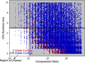
Figure 3: CPU latency for candidate configurations obtained using SeKron on a tensor $\tensorp{\bm{\mathcal{{W}}}}{}\in{\rm I\!R}^{512\times 512\times 3\times 3}$ with $S=2$ (red) and $S=3$ (blue), aiming for a speedup (e.g., $<5$ ms) and a typical compression rate (e.g., $<10\times$).

5 Conclusions

We introduced SeKron, a tensor decomposition approach using sequences of Kronecker products. SeKron allows for a wide variety of factorization structures to be achieved, while, crucially, sharing the same compression and convolution algorithms. Moreover, SeKron has been shown to generalize popular decomposition methods such as TT, TR, CP and Tucker. Thus, it mitigates the need for time-consuming development of customized convolution algorithms. Unlike other decomposition methods, SeKron is not limited to a single factorization structure, which leads to improved compressions and reduced runtimes on different hardware. Leveraging SeKron’s flexibility, we find efficient factorization structures that outperform previous decomposition methods on various image classification and super-resolution tasks.

6 Appendix

See 1

Proof.

First, we define intermediate tensors

$$\tensorp{\bm{\mathcal{{B}}}}{}_{r_{1}\cdots r_{k}}^{(k)}\triangleq\sum_{r_{k+1}}^{R_{k+1}}\tensorp{\bm{\mathcal{{A}}}}{}_{r_{1}\cdots r_{k+1}}^{(k+1)}\otimes\sum_{r_{k+2}}^{R_{k+2}}\tensorp{\bm{\mathcal{{A}}}}{}_{r_{1}\cdots r_{k+2}}^{(k+2)}\otimes\cdots\otimes\sum_{r_{S-1}}^{R_{S-1}}\tensorp{\bm{\mathcal{{A}}}}{}_{r_{1}\cdots r_{S-1}}^{(S-1)}\otimes\tensorp{\bm{\mathcal{{A}}}}{}_{r_{1}\cdots r_{S-1}}^{(S)}$$ (19)

Then the reconstruction error can be written as

$$\Bigg{\|}\tensorp{\bm{\mathcal{{W}}}}{}_{r_{1}\cdots r_{k-1}}^{(k)}-\sum_{r_{k}=1}^{\widehat{R}_{k}}\tensorp{\bm{\mathcal{{A}}}}{}^{(k)}_{r_{1}\cdots r_{k}}\otimes\tensorp{\bm{\mathcal{{B}}}}{}^{(k)}_{r_{1}\cdots r_{k}}\Bigg{\|}_{\mathrm{F}}^{2}$$ (20)

where $\tensorp{\bm{\mathcal{{W}}}}{}^{(1)}$ is the initial tensor being decomposed. As described in Section 3.2, using reshaping operations

$${\mathbf{W}}_{r_{1}\cdots r_{k-1}}^{(k)}=\textsc{Mat}(\textsc{Unfold}(\tensorp{\bm{\mathcal{{W}}}}{}_{r_{1}\cdots r_{k-1}}^{(k)},{\mathbf{d}}_{\tensorp{\bm{\mathcal{{B}}}}{}_{r_{1}\cdots r_{k}}^{(k)}})),$$ (12 revisited)

$${\mathbf{a}}_{r_{1}\cdots r_{k}}^{(k)}=\textsc{Vec}(\textsc{Unfold}(\tensorp{\bm{\mathcal{{A}}}}{}_{r_{1}\cdots r_{k}}^{(k)},{\mathbf{d}}_{\tensorp{\bm{\mathcal{{I}}}}{}_{\tensorp{\bm{\mathcal{{A}}}}{}_{r_{1}\cdots r_{k}}^{(k)}}})),\;\;{\mathbf{b}}_{r_{1}\cdots r_{k}}^{(k)}=\textsc{Vec}(\tensorp{\bm{\mathcal{{B}}}}{}_{r_{1}\cdots r_{k}}^{(k)}),$$ (13 revisited)

that preserve the sum of squares allows us to equivalently write the reconstruction error as

$$\Bigg{\|}{\mathbf{W}}_{r_{1}\cdots r_{k-1}}^{(k)}-\sum_{r_{k}=1}^{\widehat{R}_{k}}{\mathbf{a}}^{(k)}_{r_{1}\cdots r_{k}}{\mathbf{b}}^{(k)\top}_{r_{1}\cdots r_{k}}\Bigg{\|}_{\mathrm{F}}^{2}.$$ (21)

Now consider the singular value decomposition of matrix ${\mathbf{W}}_{r_{1}\cdots r_{k-1}}^{(k)}$ and let ${\mathbf{u}}_{r_{1}\cdots r_{k}}^{(k)},{\mathbf{v}}_{r_{1}\cdots r_{k}}^{(k)}$ denote its left and right singular vectors, respectively (with the right singular vector scaled according to its corresponding singlar value). Set ${\mathbf{a}}_{r_{1}\cdots r_{k}}^{(k)}={\mathbf{u}}_{r_{k}}^{(k)}$ and define and define error terms

$${\mathbf{\delta}}_{r_{1}\cdots r_{k}}^{(k)}={\mathbf{v}}_{r_{1}\cdots r_{k}}^{(k)}-{\mathbf{b}}_{r_{1}\cdots r_{k}}^{(k)},\quad\epsilon_{r_{1}\cdots r_{k}}^{(k)}=\|{\mathbf{\delta}}_{r_{1}\cdots r_{k}}^{(k)}\|.$$ (22)

Expanding out equation 21 reveals its recursive form

$$\Bigg{\|}{\mathbf{W}}_{r_{1}\cdots r_{k-1}}^{(k)} -\sum_{r_{k}=1}^{\widehat{R}_{k}}{\mathbf{a}}^{(k)}_{r_{1}\cdots r_{k}}{\mathbf{b}}^{(k)\top}_{r_{1}\cdots r_{k}}\Bigg{\|}_{\mathrm{F}}^{2}=\Bigg{\|}{\mathbf{W}}_{r_{1}\cdots r_{k-1}}^{(k)}-\sum_{r_{k}=1}^{\widehat{R}_{k}}{\mathbf{a}}^{(k)}_{r_{1}\cdots r_{k}}({\mathbf{v}}_{r_{k}}^{(k)}-{\mathbf{\delta}}_{r_{1}\cdots r_{k}}^{(k)})^{\top}\Bigg{\|}_{\mathrm{F}}^{2}$$ (23)

$$=\Bigg{\|}{\mathbf{W}}_{r_{1}\cdots r_{k-1}}^{(k)}-\sum_{r_{k}=1}^{\widehat{R}_{k}}{\mathbf{a}}^{(k)}_{r_{1}\cdots r_{k}}{\mathbf{v}}_{r_{1}\cdots r_{k}}^{(k)\top}+\sum_{r_{k}=1}^{\widehat{R}_{k}}{\mathbf{a}}^{(k)}_{r_{1}\cdots r_{k}}{\mathbf{\delta}}_{r_{1}\cdots r_{k}}^{(k)\top}\Bigg{\|}_{\mathrm{F}}^{2}$$ (24)

$$\leq\Bigg{\|}{\mathbf{W}}_{r_{1}\cdots r_{k-1}}^{(k)}-\sum_{r_{k}=1}^{\widehat{R}_{k}}{\mathbf{a}}^{(k)}_{r_{1}\cdots r_{k}}{\mathbf{v}}_{r_{1}\cdots r_{k}}^{(k)\top}\Bigg{\|}_{\mathrm{F}}^{2}+\sum_{r_{k}=1}^{\widehat{R}_{k}}\Bigg{\|}{\mathbf{a}}^{(k)}_{r_{1}\cdots r_{k}}{\mathbf{\delta}}_{r_{1}\cdots r_{k}}^{(k)\top}\Bigg{\|}_{\mathrm{F}}^{2}$$ (25)

$$\leq\Bigg{\|}{\mathbf{W}}_{r_{1}\cdots r_{k-1}}^{(k)}-\sum_{r_{k}=1}^{\widehat{R}_{k}}{\mathbf{a}}^{(k)}_{r_{1}\cdots r_{k}}{\mathbf{v}}_{r_{1}\cdots r_{k}}^{(k)\top}\Bigg{\|}_{\mathrm{F}}^{2}+\sum_{r_{k}=1}^{\widehat{R}_{k}}d^{(k)}\epsilon_{r_{1}\cdots r_{k}}^{(k)}$$ (26)

$$=\Bigg{(}\sum_{r_{k}=\widehat{R}_{k}+1}^{R_{k}}\sigma_{r_{k}}^{2}({\mathbf{W}}_{r_{1}\cdots r_{k-1}}^{(k)})\Bigg{)}+\Bigg{(}\sum_{r_{k}=1}^{\widehat{R}_{k}}d^{(k)}\epsilon_{r_{1}\cdots r_{k}}^{(k)}\Bigg{)}$$ (27)

$$=\sum_{r_{k}=\widehat{R}_{k}+1}^{R_{k}}\sigma_{r_{k}}^{2}({\mathbf{W}}_{r_{1}\cdots r_{k-1}}^{(k)})+\sum_{r_{k}=1}^{\widehat{R}_{k}}d^{(k)}\Bigg{\|}{\mathbf{v}}_{r_{1}\cdots r_{k}}^{(k)}-{\mathbf{b}}_{r_{1}\cdots r_{k}}^{(k)}\Bigg{\|}_{\mathrm{F}}^{2}$$ (28)

where $d^{(k)}\in\mathbb{N}$ is the number of dimensions of vector ${\mathbf{a}}_{r_{1}\cdots r_{k}}^{(k)}$ and $R_{k}$ is the rank of matrix ${\mathbf{W}}_{r_{1}\cdots r_{k-1}}^{(k)}$, $\sigma_{r_{k}}(\tensorp{\bm{\mathcal{{W}}}}{}_{r_{1}\cdots r_{k-1}}^{(k)})$ denotes the $r_{k}^{\text{th}}$ singular value of tensor $\tensorp{\bm{\mathcal{{W}}}}{}_{r_{1}\cdots r_{k-1}}^{(k)}$. By reshaping vectors ${\mathbf{v}}_{r_{1}\cdots r_{k}}^{(k)},{\mathbf{b}}_{r_{1}\cdots r_{k}}^{(k)}$ to matrices according to

$${\mathbf{V}}_{r_{1}\cdots r_{k}}^{(k)}=\textsc{Mat}\Bigg{(}\textsc{Unfold}\Bigg{(}\textsc{Vec}^{-1}\Bigg{(}{\mathbf{v}}_{r_{1}\cdots r_{k}}^{(k)},\prod_{s=k+1}^{S}{\mathbf{d}}^{(s)}\Bigg{)},\prod_{s=k+2}^{S}{\mathbf{d}}^{(s)}\Bigg{)}\Bigg{)},$$ (29)

$${\mathbf{B}}_{r_{1}\cdots r_{k}}^{(k)}=\textsc{Mat}\Bigg{(}\textsc{Unfold}\Bigg{(}\textsc{Vec}^{-1}\Bigg{(}{\mathbf{b}}_{r_{1}\cdots r_{k}}^{(k)},\prod_{s=k+1}^{S}{\mathbf{d}}^{(s)}\Bigg{)},\prod_{s=k+2}^{S}{\mathbf{d}}^{(s)}\Bigg{)}\Bigg{)},$$ (30)

where ${\mathbf{d}}^{(s)}=(a_{1}^{(s)},\dots,a_{N}^{(s)})$ describes the dimensions of the $s^{\text{th}}$ factor, we can re-write equation 28 as

$$\sum_{r_{k}=\widehat{R}_{k}+1}^{R_{k}} \sigma_{r_{k}}^{2}({\mathbf{W}}_{r_{1}\cdots r_{k-1}}^{(k)})+\sum_{r_{k}=1}^{\widehat{R}_{k}}d^{(k)}\Bigg{\|}{\mathbf{v}}_{r_{1}\cdots r_{k}}^{(k)}-{\mathbf{b}}_{r_{1}\cdots r_{k}}^{(k)}\Bigg{\|}_{\mathrm{F}}^{2}$$ (31)

$$=\sum_{r_{k}=\widehat{R}_{k}+1}^{R_{k}}\sigma_{r_{k}}^{2}({\mathbf{W}}_{r_{1}\cdots r_{k-1}}^{(k)})+\sum_{r_{k}=1}^{\widehat{R}_{k}}d^{(k)}\Bigg{\|}{\mathbf{V}}_{r_{1}\cdots r_{k}}^{(k)}-{\mathbf{B}}_{r_{1}\cdots r_{k}}^{(k)}\Bigg{\|}_{\mathrm{F}}^{2}$$ (32)

$$=\sum_{r_{k}=\widehat{R}_{k}+1}^{R_{k}}\sigma_{r_{k}}^{2}({\mathbf{W}}_{r_{1}\cdots r_{k-1}}^{(k)})+\sum_{r_{k}=1}^{\widehat{R}_{k}}d^{(k)}\Bigg{\|}{\mathbf{V}}_{r_{1}\cdots r_{k}}^{(k)}-\sum_{r_{k+1}=1}^{\widehat{R}_{k+1}}{\mathbf{a}}_{r_{1}\cdots r_{k+1}}^{(k+1)}{\mathbf{b}}_{r_{1}\cdots r_{k+1}}^{(k+1)\top}\Bigg{\|}_{\mathrm{F}}^{2}.$$ (33)

The last line reveals the recursive nature of the formula (compare with equation 23). Unrolling the recursive formula for $k=1,\dots,S-1$, by setting ${\mathbf{W}}_{r_{1}\cdots r_{k}}^{(k+1)}\leftarrow{\mathbf{V}}_{r_{1}\cdots r_{k}}^{(k)}$, leads to the following formula for the reconstruction error:

$$\varepsilon_{\text{SeKron}}({\mathbf{W}},{\mathbf{r}},{\mathbf{D}})=\sum_{r_{1}=\widehat{R}_{1}+1}^{R_{1}}\sigma_{r_{1}}^{2}({\mathbf{W}}^{(1)})+d^{(1)}\sum_{r_{1}=1}^{\widehat{R}_{1}}\sum_{r_{2}=\widehat{R}_{2}+1}^{R_{2}}\sigma_{r_{2}}^{2}({\mathbf{W}}_{r_{1}}^{(2)})+\cdots\\ +d^{(1)}d^{(2)}\cdots d^{(S-2)}\sum_{r_{1},r_{2},\dots,r_{S-2}=1}^{\widehat{R}_{1},\cdots,\widehat{R}_{S-2}}\sum_{r_{S-1}=\widehat{R}_{S-1}+1}^{R_{S-1}}\sigma_{r_{S-1}}^{2}({\mathbf{W}}_{r_{1}\cdots r_{S-2}}^{(S-1)})$$ (34)

where ${\mathbf{r}}=(\widehat{R}_{1},\dots,\widehat{R}_{S-1})$ contains the rank values, ${\mathbf{D}}_{s}={\mathbf{d}}^{(s)}$ contains the Kronecker factor shapes and is referred to as the ${\mathbf{D}}{\mathbf{r}}$-SeKron approximation error (note that the dependency of intermediate matrices ${\mathbf{W}}_{r_{1}\cdots r_{k-1}}^{(k)}$ on Kronecker factor shapes ${\mathbf{D}}$ is implied). Selecting $\widehat{R}_{i}=R_{i}\>\forall i$ in equation 34 results in zero reconstruction error. ∎

See 2

Proof.

The SeKron decomposition of tensor $\tensorp{\bm{\mathcal{{W}}}}{}$ is given by

$$\tensorp{\bm{\mathcal{{W}}}}{}_{i_{1}\cdots i_{N}}=\sum_{r_{1},\dots,r_{S}=1}^{R_{1},\cdots,R_{S}}\tensorp{\bm{\mathcal{{A}}}}{}_{r_{1}j_{1}^{(1)}\cdots j_{N}^{(1)}}^{(1)}\cdots\tensorp{\bm{\mathcal{{A}}}}{}_{r_{1}\cdots r_{S-1}j_{1}^{(S)}\cdots j_{N}^{(S)}}^{(S)}$$ (35)

where $\tensorp{\bm{\mathcal{{A}}}}{}^{(k)}\in{\rm I\!R}^{a_{1}^{(k)}\times\cdots a_{N}^{(k)}}$ and

$$j_{n}^{(k)}=\begin{cases}i_{n}-\sum_{t=1}^{k-2}j_{n}^{(t)}\prod_{l=t+1}^{S}a_{n}^{(l)}\text{mod}\,a_{n}^{(S)}\quad&k=S,\\ \left\lfloor\frac{i_{n}-\sum_{t=1}^{k-1}j_{n}^{(t)}\prod_{l=t+1}^{S}a_{n}^{(l)}}{\prod_{l=k+1}^{S}a_{n}^{(l)}}\right\rfloor\quad&\text{otherwise},\end{cases}$$ (6 revisted)

The CP decomposition of tensor $\tensorp{\bm{\mathcal{{W}}}}{}$ in scalar form is

$$\tensorp{\bm{\mathcal{{W}}}}{}_{i_{1}\cdots i_{N}}=\sum_{r=1}^{R^{(\text{CP})}}\tensorp{\bm{\mathcal{{A}}}}{}_{ri_{1}}^{(\text{CP}_{1})}\cdots\tensorp{\bm{\mathcal{{A}}}}{}_{ri_{N}}^{(\text{CP}_{N})}$$ (36)

where $\tensorp{\bm{\mathcal{{A}}}}{}^{(\text{CP}_{k})}\in{\rm I\!R}^{R^{(\text{CP})}\times w_{k}}$. Configuring the SeKron decomposition in equation 35 such that $S=N;\;R_{1}=R^{(\text{CP})};\;R_{2},\dots,R_{N}=1$ and $a_{n}^{(n)}=w_{n}$ for $n=1,\dots,N$ leads to the equivalent form

$$\tensorp{\bm{\mathcal{{W}}}}{}_{i_{1}\cdots i_{N}}=\sum_{r_{1}=1}^{R^{(\text{CP})}}\tensorp{\bm{\mathcal{{A}}}}{}_{r_{1}i_{1}1\cdots 1}^{(1)}\cdots\tensorp{\bm{\mathcal{{A}}}}{}_{r_{,}1\cdots 1i_{N}}^{(N)}.$$ (37)

The Tucker decomposition of tensor $\tensorp{\bm{\mathcal{{W}}}}{}$ is given by

$$\tensorp{\bm{\mathcal{{W}}}}{}_{i_{1}\cdots i_{N}}=\sum_{r_{1}=1,\dots,r_{N}}^{R_{1}^{(\text{T})},\dots R_{N}^{(\text{T})}}\tensorp{\bm{\mathcal{{G}}}}{}_{r_{1}\cdots r_{N}}\tensorp{\bm{\mathcal{{A}}}}{}_{i_{1}r_{1}}^{(\text{T}_{1})}\cdots\tensorp{\bm{\mathcal{{A}}}}{}_{i_{N}r_{N}}^{(\text{T}_{N})}$$ (38)

where $\tensorp{\bm{\mathcal{{G}}}}{}\in{\rm I\!R}^{R_{1}^{(\text{T})}\times\cdots\times R_{N}^{(\text{T})}}$ and $\tensorp{\bm{\mathcal{{A}}}}{}^{(\text{T}_{k})}\in{\rm I\!R}^{w_{k}\times R_{k}^{(\text{T})}}$. The SeKron decomposition of tensor $\tensorp{\bm{\mathcal{{W}}}}{}$, with $S=N+1,\;R_{n}=R_{n}^{(T)}$ and $a_{n}^{(n)}=w_{n}$ for $n=1,\dots,N$ yields

$$\tensorp{\bm{\mathcal{{W}}}}{}_{i_{1}\cdots i_{N}}=\sum_{r_{1},\dots,r_{N}=1}^{R_{1}^{(\text{T})},\cdots,R_{N}^{(\text{T})}}\tensorp{\bm{\mathcal{{A}}}}{}_{r_{1}i_{1}1\cdots 1}^{(1)}\cdots\tensorp{\bm{\mathcal{{A}}}}{}_{r_{1}\cdots r_{N}1\cdots 1i_{N}}^{(N)}\tensorp{\bm{\mathcal{{A}}}}{}_{r_{1}\cdots r_{N}1\cdots 1}^{(N+1)},$$ (39)

which is equivalent to equation 38 in the special case where there are nullity constraints on some elements in the Kronecker factors, such that for $k=2,\dots,N$

$$\tensorp{\bm{\mathcal{{A}}}}{}^{(k)}_{r_{1}\cdots r_{k}1\cdots 1i_{k}1\cdots 1}=0\quad\text{when}\quad r_{j}\in\{x\in\mathbb{N}\;|\;x\leq R_{j}^{(\text{T})},\;x\neq R_{j}^{(\text{T}^{*})}\}\quad j=1,\dots,k-1$$ (40)

for any choice of $R_{j}^{(\text{T}*)}\in\{x\in\mathbb{N}\;|\;x\leq R_{j}^{(\text{T})}\}$. The Tensor Ring (TR) decomposition of $\tensorp{\bm{\mathcal{{W}}}}{}$ is given by

$$\tensorp{\bm{\mathcal{{W}}}}{}_{i_{1}\cdots i_{N}}=\sum_{r_{1}=1,\dots,r_{N}}^{R_{1}^{(\text{TR})},\dots R_{N}^{(\text{TR})}}\tensorp{\bm{\mathcal{{A}}}}{}_{i_{1}r_{1}r_{2}}^{(\text{TR}_{1})}\cdots\tensorp{\bm{\mathcal{{A}}}}{}_{i_{N}r_{N}r_{N+1}}^{(\text{TR}_{N})}$$ (41)

where $\tensorp{\bm{\mathcal{{A}}}}{}^{(\text{TR}_{k})}\in{\rm I\!R}^{w_{k}\times R_{k}^{(\text{TR})}\times R_{k+1}^{(\text{TR})}}$, and $R_{1}^{(\text{TR})}=R_{N+1}^{(\text{TR})}$. As the Tensor Train decomposition can be viewed as a special case of the Tensor Ring decomposition (with $R_{1}^{(\text{TR})}=R_{N+1}^{(\text{TR})}=1$), it suffices to show that SeKron generalizes Tensor Ring. The SeKron decomposition of tensor $\tensorp{\bm{\mathcal{{W}}}}{}$, with $S=N+1$; $R_{k}=R_{k}^{(\text{TR})}$ for $k=1,\dots,N-1$ and $a_{n}^{(n+1)}=w_{n}$ for $n=1,\dots,N$ leads to

$$\tensorp{\bm{\mathcal{{W}}}}{}_{i_{1}\cdots i_{N}}=\sum_{r_{1},\dots,r_{N}=1}^{R_{1}^{(\text{TR)}},\dots,R_{N}^{(\text{TR})}}\tensorp{\bm{\mathcal{{A}}}}{}_{r_{1}1\cdots 1}^{(1)}\tensorp{\bm{\mathcal{{A}}}}{}_{r_{1}r_{2}i_{1}1\cdots 1}^{(2)}\cdots\tensorp{\bm{\mathcal{{A}}}}{}_{r_{1}\cdots r_{N+1}1\cdots 1i_{N}}^{(N+1)},$$ (42)

which is equivalent to equation 41 in the special case where some elements in the Kronecker factors are constrained, such that all elements in tensor $\tensorp{\bm{\mathcal{{A}}}}{}^{(1)}$ are constrained to one and

$$\tensorp{\bm{\mathcal{{A}}}}{}^{(k)}_{r_{1}\cdots r_{k}1\cdots 1i_{k}1\cdots 1}=0\quad\forall r_{j}\in\{x\in\mathbb{N}\;|\;x\leq R_{j}^{(\text{TR})},\;x\neq R_{j}^{(\text{TR}^{*})}\}$$ (43)

for

$$j=\begin{cases}1,\dots,k-2&k=2,\dots,N\\ 2,\dots,k-1&k=N+1\end{cases}$$ (44)

for any choice of $R_{j}^{(\text{TR}^{*})}\in\{x\in\mathbb{N}\;|\;x\leq R_{j}^{(\text{TR})}\}$. ∎

See 3

Proof.

First we bring out the summations in the SeKron representaion of $\tensorp{\bm{\mathcal{{W}}}}{}$

$$\tensorp{\bm{\mathcal{{W}}}}{}=\sum_{r_{1}}^{R_{1}}\tensorp{\bm{\mathcal{{A}}}}{}_{r_{1}}^{(1)}\otimes\sum_{r_{2}}^{R_{2}}\tensorp{\bm{\mathcal{{A}}}}{}_{r_{1}r_{2}}^{(2)}\otimes\cdots\otimes\sum_{r_{S-1}}^{R_{S-1}}\tensorp{\bm{\mathcal{{A}}}}{}_{r_{1}\cdots r_{S-1}}^{(S-1)}\otimes\tensorp{\bm{\mathcal{{A}}}}{}_{r_{1}\cdots r_{S-1}}^{(S)},$$ (8 revisted)

such that

$$\tensorp{\bm{\mathcal{{W}}}}{}=\sum_{r_{1},\dots,r_{S}=1}^{R_{1},\cdots,R_{S-1}}\tensorp{\bm{\mathcal{{A}}}}{}_{r_{1}}^{(1)}\otimes\dots\otimes\tensorp{\bm{\mathcal{{A}}}}{}_{r_{1}r_{2}\cdots r_{S-1}}^{(S)}.$$ (45)

Then, using the scalar form definition of sequences of kronecker products in equation 6

$$j_{n}^{(k)}=\begin{cases}i_{n}-\sum_{t=1}^{k-2}j_{n}^{(t)}\prod_{l=t+1}^{S}a_{n}^{(l)}\text{mod}\,a_{n}^{(S)}\quad&k=S,\\ \left\lfloor\frac{i_{n}-\sum_{t=1}^{k-1}j_{n}^{(t)}\prod_{l=t+1}^{S}a_{n}^{(l)}}{\prod_{l=k+1}^{S}a_{n}^{(l)}}\right\rfloor\quad&\text{otherwise},\end{cases}$$ (6 revisited)

allows us to re-write equation 45 in scalar form as

$$\tensorp{\bm{\mathcal{{W}}}}{}_{i_{1}\cdots i_{N}}=\sum_{r_{1}\cdots r_{S}=1}^{R_{1}}\tensorp{\bm{\mathcal{{A}}}}{}_{r_{1}j_{1}^{(1)}\cdots j_{N}^{(1)}}^{(1)}\cdots\tensorp{\bm{\mathcal{{A}}}}{}_{r_{1}\cdots r_{S-1}j_{1}^{(S)}\cdots j_{N}^{(S)}}^{(S)}$$ (46)

As the $j_{n}^{(k)}$ terms decompose $i_{n}$ into an integer weighted sum, we can recover $i_{n}$ using

$$i_{n}=f({\mathbf{j}}_{n})\triangleq\sum_{k=1}^{S}j_{n}^{(k)}\prod_{l=k+1}^{S}a_{n}^{(l)},$$ (47)

where ${\mathbf{j}}_{n}=(j_{n}^{(1)},\dots,j_{n}^{(S)})$. Thus, we can write

$$\tensorp{\bm{\mathcal{{X}}}}{}_{i_{1}+z_{1},\cdots i_{N}+z_{N}}=\tensorp{\bm{\mathcal{{X}}}}{}_{f({\mathbf{j}}_{1})+z_{1},\cdots f({\mathbf{j}}_{N})+z_{N}}.$$ (48)

Finally, combining equations equation 46 and equation 48 leads to equation 16. ∎

Theorem 4.

(Universal approximation via shallow SeKron networks) Any shallow SeKron factorized neural network $\hat{f}^{(s)}$ with an $L$-Lipschitz activation function $a$, is dense in the class of continuous functions $C(X)$ for any compact subset $X$ of ${\rm I\!R}^{d}$

Proof.

Let $\hat{f}$ denote a shallow neural network, and $f\in C(X)$. Then,

$$\left\|f-\hat{f}^{(s)}\right\|_{2}^{2} \triangleq\int_{X}\Bigg{(}f(x)-\hat{f}^{(s)}(x)\Bigg{)}^{2}d\mu$$ (49)

$$=\int_{X}\Bigg{(}f(x)-\hat{f}(x)\Bigg{)}^{2}d\mu$$ (50)

$$+\int_{X}\Bigg{(}\hat{f}(x)-\hat{f}^{(s)}(x)\Bigg{)}^{2}d\mu$$ (51)

$$+2\int_{X}\Bigg{(}f(x)-\hat{f}(x)\Bigg{)}\Bigg{(}\hat{f}(x)-\hat{f}^{(s)}(x)\Bigg{)}d\mu$$ (52)

According to Hornik (1991), equation 50 is dense in $C(X)$; therefore, it suffices to show that equation 51 is bounded as well.

$$\int_{X}\Bigg{(}\hat{f}(x)-\hat{f}^{(s)}(x)\Bigg{)}^{2}d\mu =\int_{X}\Bigg{(}{\mathbf{w}}^{\top}{\mathbf{a}}({\mathbf{W}}{\mathbf{x}})-{\mathbf{w}}^{\top}{\mathbf{a}}({\mathbf{W}}^{(s)}{\mathbf{x}})\Bigg{)}^{2}d\mu$$ (53)

$$\leq L\big{\|}{\mathbf{w}}\big{\|}_{2}^{2}\big{\|}X\big{\|}_{2}^{2}\,\varepsilon_{\text{SeKron}}({\mathbf{W}},{\mathbf{r}},{\mathbf{D}})$$ (54)

where $\varepsilon$ denotes the ${\mathbf{D}}{\mathbf{r}}$-SeKron approximation error as in equation 34, with matrix ${\mathbf{D}}$ and vector ${\mathbf{r}}$ describing the shapes of the Kronecker factors the ranks used in the SeKron decomposition of ${\mathbf{W}}$, respectively. ∎

References

• Afshar et al. (2021) Ardavan Afshar, Kejing Yin, Sherry Yan, Cheng Qian, Joyce Ho, Haesun Park, and Jimeng Sun. Swift: scalable wasserstein factorization for sparse nonnegative tensors. In Proceedings of the AAAI Conference on Artificial Intelligence, volume 35, pp.  6548–6556, 2021.
• Agustsson & Timofte (2017) Eirikur Agustsson and Radu Timofte. NTIRE 2017 challenge on single image super-resolution: Dataset and study. In IEEE Conference on Computer Vision and Pattern Recognition Workshops (CVPRW), pp.  1122–1131, 2017.
• Alvarez & Salzmann (2017) Jose M Alvarez and Mathieu Salzmann. Compression-aware training of deep networks. In Advances in Neural Information Processing Systems, 2017.
• Bevilacqua et al. (2012) Marco Bevilacqua, Aline Roumy, Christine Guillemot, and Marie line Alberi Morel. Low-complexity single-image super-resolution based on nonnegative neighbor embedding. In British Machine Vision Conference, pp.  135.1–135.10, 2012.
• Boulch (2018) Alexandre Boulch. Reducing parameter number in residual networks by sharing weights. Pattern Recognition Letters, 103:53–59, 2018.
• Chollet (2017) François Chollet. Xception: Deep learning with depthwise separable convolutions. In IEEE Conference on Computer Vision and Pattern Recognition, pp.  1251–1258, 2017.
• Courbariaux et al. (2015) Matthieu Courbariaux, Yoshua Bengio, and Jean-Pierre David. Binaryconnect: Training deep neural networks with binary weights during propagations. Advances in Neural Information Processing Systems, 28, 2015.
• Courbariaux et al. (2016) Matthieu Courbariaux, Itay Hubara, Daniel Soudry, Ran El-Yaniv, and Yoshua Bengio. Binarized neural networks: Training deep neural networks with weights and activations constrained to +1 or -1. arXiv preprint arXiv:1602.02830, 2016.
• Denil et al. (2013) Misha Denil, Babak Shakibi, Laurent Dinh, Marc’Aurelio Ranzato, and Nando de Freitas. Predicting parameters in deep learning. In Advances in Neural Information Processing Systems, 2013.
• Garipov et al. (2016) Timur Garipov, Dmitry Podoprikhin, Alexander Novikov, and Dmitry P. Vetrov. Ultimate tensorization: compressing convolutional and FC layers alike. CoRR, abs/1611.03214, 2016.
• Gysel et al. (2018) Philipp Gysel, Jon Pimentel, Mohammad Motamedi, and Soheil Ghiasi. Ristretto: A framework for empirical study of resource-efficient inference in convolutional neural networks. IEEE Transactions on Neural Networks and Learning Systems, 29(11):5784–5789, 2018.
• Hameed et al. (2022) Marawan Gamal Abdel Hameed, Marzieh S. Tahaei, Ali Mosleh, and Vahid Partovi Nia. Convolutional neural network compression through generalized Kronecker product decomposition. In AAAI Conference on Artificial Intelligence, 2022.
• Han et al. (2015a) Song Han, Huizi Mao, and William J Dally. Deep compression: Compressing deep neural networks with pruning, trained quantization and Huffman coding. arXiv preprint arXiv:1510.00149, 2015a.
• Han et al. (2015b) Song Han, Jeff Pool, John Tran, and William Dally. Learning both weights and connections for efficient neural network. Advances in Neural Information Processing Systems, 28, 2015b.
• Harshman et al. (1970) Richard A Harshman et al. Foundations of the parafac procedure: Models and conditions for an" explanatory" multimodal factor analysis. 1970.
• He et al. (2016) Kaiming He, Xiangyu Zhang, Shaoqing Ren, and Jian Sun. Deep residual learning for image recognition. In IEEE Conference on Computer Vision and Pattern Recognition (CVPR), pp.  770–778, 2016.
• He et al. (2018) Yang He, Guoliang Kang, Xuanyi Dong, Yanwei Fu, and Yi Yang. Soft filter pruning for accelerating deep convolutional neural networks. arXiv preprint arXiv:1808.06866, 2018.
• He et al. (2020) Yang He, Yuhang Ding, Ping Liu, Linchao Zhu, Hanwang Zhang, and Yi Yang. Learning filter pruning criteria for deep convolutional neural networks acceleration. In IEEE/CVF Conference on Computer Vision and Pattern Recognition (CVPR), 2020.
• He et al. (2017) Yihui He, Xiangyu Zhang, and Jian Sun. Channel pruning for accelerating very deep neural networks. In IEEE International Conference on Computer Vision, pp. 1389–1397, 2017.
• Heo et al. (2019) Byeongho Heo, Minsik Lee, Sangdoo Yun, and Jin Young Choi. Knowledge distillation with adversarial samples supporting decision boundary. In AAAI Conference on Artificial Intelligence, pp. 3771–3778, 2019.
• Hinton et al. (2015) Geoffrey E. Hinton, Oriol Vinyals, and Jeffrey Dean. Distilling the knowledge in a neural network. CoRR, abs/1503.02531, 2015.
• Hong et al. (2020) David Hong, Tamara G Kolda, and Jed A Duersch. Generalized canonical polyadic tensor decomposition. SIAM Review, 62(1):133–163, 2020.
• Howard et al. (2019) Andrew Howard, Mark Sandler, Grace Chu, Liang-Chieh Chen, Bo Chen, Mingxing Tan, Weijun Wang, Yukun Zhu, Ruoming Pang, Vijay Vasudevan, et al. Searching for MobileNetV3. In IEEE/CVF International Conference on Computer Vision, pp. 1314–1324, 2019.
• Huang et al. (2015) Jia-Bin Huang, Abhishek Singh, and Narendra Ahuja. Single image super-resolution from transformed self-exemplars. In IEEE Conference on Computer Vision and Pattern Recognition (CVPR), June 2015.
• Hubara et al. (2017) Itay Hubara, Matthieu Courbariaux, Daniel Soudry, Ran El-Yaniv, and Yoshua Bengio. Quantized neural networks: Training neural networks with low precision weights and activations. The Journal of Machine Learning Research, 18(1):6869–6898, 2017.
• Iandola et al. (2016) Forrest N Iandola, Song Han, Matthew W Moskewicz, Khalid Ashraf, William J Dally, and Kurt Keutzer. Squeezenet: Alexnet-level accuracy with 50x fewer parameters and $<$ 0.5 MB model size. arXiv preprint arXiv:1602.07360, 2016.
• Idelbayev & Carreira-Perpinan (2020) Yerlan Idelbayev and Miguel A. Carreira-Perpinan. Low-rank compression of neural nets: Learning the rank of each layer. In IEEE/CVF Conference on Computer Vision and Pattern Recognition (CVPR), June 2020.
• Jacob et al. (2018) Benoit Jacob, Skirmantas Kligys, Bo Chen, Menglong Zhu, Matthew Tang, Andrew Howard, Hartwig Adam, and Dmitry Kalenichenko. Quantization and training of neural networks for efficient integer-arithmetic-only inference. In IEEE Conference on Computer Vision and Pattern Recognition, pp.  2704–2713, 2018.
• Jaderberg et al. (2014) Max Jaderberg, Andrea Vedaldi, and Andrew Zisserman. Speeding up convolutional neural networks with low rank expansions. arXiv preprint arXiv:1405.3866, 2014.
• Kim et al. (2015) Yong-Deok Kim, Eunhyeok Park, Sungjoo Yoo, Taelim Choi, Lu Yang, and Dongjun Shin. Compression of deep convolutional neural networks for fast and low power mobile applications. arXiv preprint arXiv:1511.06530, 2015.
• Kim et al. (2016) Yong-Deok Kim, Eunhyeok Park, Sungjoo Yoo, Taelim Choi, Lu Yang, and Dongjun Shin. Compression of deep convolutional neural networks for fast and low power mobile applications. In International Conference on Learning Representations, 2016.
• Kokkinos & Lefkimmiatis (2018) Filippos Kokkinos and Stamatios Lefkimmiatis. Deep image demosaicking using a cascade of convolutional residual denoising networks. In European Conference on Computer Vision (ECCV), pp. 303–319, 2018.
• Krizhevsky (2009) Alex Krizhevsky. Learning multiple layers of features from tiny images. Technical report, 2009.
• Krizhevsky et al. (2012) Alex Krizhevsky, Ilya Sutskever, and Geoffrey E. Hinton. ImageNet classification with deep convolutional neural networks. In Advances in Neural Information Processing Systems, pp. 1106–1114, 2012.
• Lebedev et al. (2015) Vadim Lebedev, Yaroslav Ganin, Maksim Rakhuba, Ivan V. Oseledets, and Victor S. Lempitsky. Speeding-up convolutional neural networks using fine-tuned CP-decomposition. In International Conference on Learning Representations, 2015.
• Ledig et al. (2017) Christian Ledig, Lucas Theis, Ferenc Huszár, Jose Caballero, Andrew Cunningham, Alejandro Acosta, Andrew Aitken, Alykhan Tejani, Johannes Totz, Zehan Wang, et al. Photo-realistic single image super-resolution using a generative adversarial network. In IEEE Conference on Computer Vision and Pattern Recognition, pp.  4681–4690, 2017.
• Li et al. (2016) Fengfu Li, Bo Zhang, and Bin Liu. Ternary weight networks. arXiv preprint arXiv:1605.04711, 2016.
• Li et al. (2017) Hao Li, Asim Kadav, Igor Durdanovic, Hanan Samet, and Hans Peter Graf. Pruning filters for efficient ConvNets. In International Conference on Learning Representations, 2017.
• Li et al. (2019) Yawei Li, Shuhang Gu, Luc Van Gool, and Radu Timofte. Learning filter basis for convolutional neural network compression. In IEEE International Conference on Computer Vision, 2019.
• Liebenwein et al. (2020) Lucas Liebenwein, Cenk Baykal, Harry Lang, Dan Feldman, and Daniela Rus. Provable filter pruning for efficient neural networks. In International Conference on Learning Representations, 2020.
• Liebenwein et al. (2021) Lucas Liebenwein, Alaa Maalouf, Dan Feldman, and Daniela Rus. Compressing neural networks: Towards determining the optimal layer-wise decomposition. In Advances in Neural Information Processing Systems, 2021.
• Lim et al. (2017) Bee Lim, Sanghyun Son, Heewon Kim, Seungjun Nah, and Kyoung Mu Lee. Enhanced deep residual networks for single image super-resolution. In The IEEE Conference on Computer Vision and Pattern Recognition (CVPR) Workshops, July 2017.
• Liu et al. (2015) Baoyuan Liu, Min Wang, Hassan Foroosh, Marshall Tappen, and Marianna Pensky. Sparse convolutional neural networks. In IEEE Conference on Computer Vision and Pattern Recognition, pp.  806–814, 2015.
• Liu et al. (2019) Zechun Liu, Haoyuan Mu, Xiangyu Zhang, Zichao Guo, Xin Yang, Kwang-Ting Cheng, and Jian Sun. Metapruning: Meta learning for automatic neural network channel pruning. In IEEE International Conference on Computer Vision, pp. 3296–3305, 2019.
• Louizos et al. (2018) Christos Louizos, Matthias Reisser, Tijmen Blankevoort, Efstratios Gavves, and Max Welling. Relaxed quantization for discretized neural networks. arXiv preprint arXiv:1810.01875, 2018.
• Luo et al. (2017) Jian-Hao Luo, Jianxin Wu, and Weiyao Lin. ThiNet: A filter level pruning method for deep neural network compression. In IEEE International Conference on Computer Vision, pp. 5058–5066, 2017.
• Martin et al. (2001) D. Martin, C. Fowlkes, D. Tal, and J. Malik. A database of human segmented natural images and its application to evaluating segmentation algorithms and measuring ecological statistics. In IEEE International Conference on Computer Vision, volume 2, pp.  416–423 vol.2, 2001.
• Mirzadeh et al. (2020) Seyed-Iman Mirzadeh, Mehrdad Farajtabar, Ang Li, Nir Levine, Akihiro Matsukawa, and Hassan Ghasemzadeh. Improved knowledge distillation via teacher assistant. In AAAI Conference on Artificial Intelligence, pp. 5191–5198, 2020.
• Novikov et al. (2015) Alexander Novikov, Dmitrii Podoprikhin, Anton Osokin, and Dmitry P Vetrov. Tensorizing neural networks. In C. Cortes, N. Lawrence, D. Lee, M. Sugiyama, and R. Garnett (eds.), Advances in Neural Information Processing Systems, 2015.
• Oseledets (2011) Ivan V Oseledets. Tensor-train decomposition. SIAM Journal on Scientific Computing, 33(5):2295–2317, 2011.
• Phan et al. (2020) Anh-Huy Phan, Konstantin Sobolev, Konstantin Sozykin, Dmitry Ermilov, Julia Gusak, Petr Tichavskỳ, Valeriy Glukhov, Ivan Oseledets, and Andrzej Cichocki. Stable low-rank tensor decomposition for compression of convolutional neural network. In European Conference on Computer Vision, pp.  522–539. Springer, 2020.
• Rastegari et al. (2016) Mohammad Rastegari, Vicente Ordonez, Joseph Redmon, and Ali Farhadi. Xnor-net: ImageNet classification using binary convolutional neural networks. In European Conference on Computer Vision, pp.  525–542. Springer, 2016.
• Ren et al. (2015) Shaoqing Ren, Kaiming He, Ross Girshick, and Jian Sun. Faster R-CNN: Towards real-time object detection with region proposal networks. Advances in Neural Information Processing Systems, 28:91–99, 2015.
• Sandler et al. (2018) Mark Sandler, Andrew Howard, Menglong Zhu, Andrey Zhmoginov, and Liang-Chieh Chen. Mobilenetv2: Inverted residuals and linear bottlenecks. In IEEE Conference on Computer Vision and Pattern Recognition, pp.  4510–4520, 2018.
• Schuler et al. (2015) Christian J Schuler, Michael Hirsch, Stefan Harmeling, and Bernhard Schölkopf. Learning to deblur. IEEE Transactions on Pattern Analysis and Machine Intelligence, 38(7):1439–1451, 2015.
• Tan & Le (2019) Mingxing Tan and Quoc Le. EfficientNet: Rethinking model scaling for convolutional neural networks. In International Conference on Machine Learning, pp. 6105–6114. PMLR, 2019.
• Tang et al. (2017) Wei Tang, Gang Hua, and Liang Wang. How to train a compact binary neural network with high accuracy? In AAAI Conference on Artificial Intelligence, 2017.
• Thakker et al. (2019) Urmish Thakker, Jesse Beu, Dibakar Gope, Chu Zhou, Igor Fedorov, Ganesh Dasika, and Matthew Mattina. Compressing RNNs for IoT devices by 15-38x using Kronecker products. arXiv preprint arXiv:1906.02876, 2019.
• Tucker (1963) Ledyard R Tucker. Implications of factor analysis of three-way matrices for measurement of change. Problems in Measuring Change, 15(122-137):3, 1963.
• Uhlich et al. (2019) Stefan Uhlich, Lukas Mauch, Fabien Cardinaux, Kazuki Yoshiyama, Javier Alonso Garcia, Stephen Tiedemann, Thomas Kemp, and Akira Nakamura. Mixed precision DNNs: All you need is a good parametrization. In International Conference on Learning Representations, 2019.
• Wang et al. (2017) Wenqi Wang, Vaneet Aggarwal, and Shuchin Aeron. Efficient low rank tensor ring completion. In IEEE International Conference on Computer Vision, pp. 5697–5705, 2017.
• Wang et al. (2018a) Wenqi Wang, Yifan Sun, Brian Eriksson, Wenlin Wang, and Vaneet Aggarwal. Wide compression: Tensor ring nets. In IEEE Conference on Computer Vision and Pattern Recognition (CVPR), June 2018a.
• Wang et al. (2018b) Xintao Wang, Ke Yu, Shixiang Wu, Jinjin Gu, Yihao Liu, Chao Dong, Yu Qiao, and Chen Change Loy. ESRGAN: Enhanced super-resolution generative adversarial networks. In European Conference on European Conference Vision (ECCV), pp.  0–0, 2018b.
• Wen et al. (2016) Wei Wen, Chunpeng Wu, Yandan Wang, Yiran Chen, and Hai Li. Learning structured sparsity in deep neural networks. Advances in Neural Information Processing Systems, 29, 2016.
• Yang et al. (2020) Yingzhen Yang, Jiahui Yu, Nebojsa Jojic, Jun Huan, and Thomas S. Huang. Fsnet: Compression of deep convolutional neural networks by filter summary. In International Conference on Learning Representations, 2020.
• Yin et al. (2021) Miao Yin, Yang Sui, Siyu Liao, and Bo Yuan. Towards efficient tensor decomposition-based DNN model compression with optimization framework. In IEEE/CVF Conference on Computer Vision and Pattern Recognition (CVPR), pp.  10674–10683, June 2021.
• Zagoruyko & Komodakis (2016) Sergey Zagoruyko and Nikos Komodakis. Wide residual networks. arXiv preprint arXiv:1605.07146, 2016.
• Zeyde et al. (2012) Roman Zeyde, Michael Elad, and Matan Protter. On single image scale-up using sparse-representations. In Jean-Daniel Boissonnat, Patrick Chenin, Albert Cohen, Christian Gout, Tom Lyche, Marie-Laurence Mazure, and Larry Schumaker (eds.), Curves and Surfaces, pp.  711–730, 2012.
• Zhang et al. (2018a) Dongqing Zhang, Jiaolong Yang, Dongqiangzi Ye, and Gang Hua. LQ-nets: Learned quantization for highly accurate and compact deep neural networks. In European Conference on Computer Vision (ECCV), pp. 365–382, 2018a.
• Zhang et al. (2018b) Tianyun Zhang, Shaokai Ye, Kaiqi Zhang, Jian Tang, Wujie Wen, Makan Fardad, and Yanzhi Wang. A systematic DNN weight pruning framework using alternating direction method of multipliers. In European Conference on Computer Vision (ECCV), pp. 184–199, 2018b.
• Zhang et al. (2016) Xiangyu Zhang, Jianhua Zou, Kaiming He, and Jian Sun. Accelerating very deep convolutional networks for classification and detection. IEEE Transactions on Pattern Analysis and Machine Intelligence, 38(10):1943–1955, 2016.
• Zhang et al. (2018c) Xiangyu Zhang, Xinyu Zhou, Mengxiao Lin, and Jian Sun. ShuffleNet: An extremely efficient convolutional neural network for mobile devices. In IEEE Conference on Computer Vision and Pattern Recognition, pp.  6848–6856, 2018c.
• Zheng et al. (2021) Yu-Bang Zheng, Ting-Zhu Huang, Xi-Le Zhao, Qibin Zhao, and Tai-Xiang Jiang. Fully-connected tensor network decomposition and its application to higher-order tensor completion. In Proceedings of the AAAI Conference on Artificial Intelligence, volume 35, pp.  11071–11078, 2021.
• Zhou et al. (2016) Hao Zhou, Jose M Alvarez, and Fatih Porikli. Less is more: Towards compact CNNs. In European Conference on Computer Vision, pp.  662–677, 2016.
• Zhou et al. (2015) Shuchang Zhou, Jia-Nan Wu, Yuxin Wu, and Xinyu Zhou. Exploiting local structures with the kronecker layer in convolutional networks. arXiv preprint arXiv:1512.09194, 2015.
• Zhu et al. (2016) Chenzhuo Zhu, Song Han, Huizi Mao, and William J Dally. Trained ternary quantization. arXiv preprint arXiv:1612.01064, 2016.
• Zhuang et al. (2018) Zhuangwei Zhuang, Mingkui Tan, Bohan Zhuang, Jing Liu, Yong Guo, Qingyao Wu, Junzhou Huang, and Jinhui Zhu. Discrimination-aware channel pruning for deep neural networks. Advances in Neural Information Processing Systems, 31, 2018.