Contrastive Neural Ratio Estimation

Abstract

Likelihood-to-evidence ratio estimation is usually cast as either a binary (nre-a) or a multiclass (nre-b) classification task. In contrast to the binary classification framework, the current formulation of the multiclass version has an intrinsic and unknown bias term, making otherwise informative diagnostics unreliable. We propose a multiclass framework free from the bias inherent to nre-b at optimum, leaving us in the position to run diagnostics that practitioners depend on. It also recovers nre-a in one corner case and nre-b in the limiting case. For fair comparison, we benchmark the behavior of all algorithms in both familiar and novel training regimes: when jointly drawn data is unlimited, when data is fixed but prior draws are unlimited, and in the commonplace fixed data and parameters setting. Our investigations reveal that the highest performing models are distant from the competitors (nre-a, nre-b) in hyperparameter space. We make a recommendation for hyperparameters distinct from the previous models. We suggest a bound on the mutual information as a performance metric for simulation-based inference methods, without the need for posterior samples, and provide experimental results.

1 Introduction

Figure 1: Conceptual, interpolated map from investigated hyperparameters of proposed algorithm nre-c to a measurement of posterior exactness using the Classifier Two-Sample Test. Best 0.5, worst 1.0. Red dot indicates nre-a’s hyperparameters, $\gamma=1$ and $K=1$ [30]. Purple line implies nre-b [16] with $\gamma=\infty$ and $K\geq 1$. nre-c covers the entire plane, generalizing other methods. Best performance occurs with $K>1$ and $\gamma\approx 1$, in contrast with the settings of existing algorithms.

We begin with a motivating example: Consider the task of inferring the mass of an exoplanet $\boldsymbol{\theta}_{o}$ from the light curve observations $\boldsymbol{x}_{o}$ of a distant star. We design a computer program that maps hypothetical mass $\boldsymbol{\theta}$ to a simulated light curve $\boldsymbol{x}$ using relevant physical theory. Our simulator computes $\boldsymbol{x}$ from $\boldsymbol{\theta}$, but the inverse mapping is unspecified and likely intractable. Simulation-based inference (sbi) puts this problem in a probabilistic context [64, 13]. Although we cannot analytically evaluate it, we assume that the simulator is sampling from the conditional probability distribution $p(\boldsymbol{x}\,|\,\boldsymbol{\theta})$. After specifying a prior $p(\boldsymbol{\theta})$, the inverse amounts to estimating the posterior $p(\boldsymbol{\theta}\,|\,\boldsymbol{x}_{o})$. This problem setting occurs across scientific domains [10, 1, 7, 29, 11] where $\boldsymbol{\theta}$ generally represents input parameters of the simulator and $\boldsymbol{x}$ the simulated output observation. Our design goal is to produce a surrogate model $\hat{p}(\boldsymbol{\theta}\,|\,\boldsymbol{x})$ approximating the posterior for any data $\boldsymbol{x}$ while limiting excessive simulation.

Figure 2: Schematic depicts how the loss is computed in nre algorithms. ($\boldsymbol{\theta}$, $\boldsymbol{x}$) pairs are sampled from distributions at the top of the figure, entering the loss functions as depicted. nre-c controls the number of contrastive classes with $K$ and the weight of independent and dependent terms with $p_{0}$ and $p_{K}$. nre-c generalizes other algorithms. Hyperparameters recovering nre-a and nre-b are listed next to the name within the dashed areas. Notation details are defined in Section 2.1.

Density estimation [5, 54, 55] can fit the likelihood [15, 56, 2, 43] or posterior [6, 53, 42, 21] directly; however, an appealing alternative for practitioners is estimating a ratio between distributions [34, 12, 69, 30, 16]. Specifically, the likelihood-to-evidence ratio $\frac{p(\boldsymbol{\theta}\,|\,\boldsymbol{x})}{p(\boldsymbol{\theta})}=\frac{p(\boldsymbol{x}\,|\,\boldsymbol{\theta})}{p(\boldsymbol{x})}=\frac{p(\boldsymbol{\theta},\boldsymbol{x})}{p(\boldsymbol{\theta})p(\boldsymbol{x})}$. Unlike the other methods, ratio estimation enables easy aggregation of independent and identically drawn data $\boldsymbol{x}$. Ratio and posterior estimation can compute bounds on the mutual information and an importance sampling diagnostic.

Estimating $\frac{p(\boldsymbol{x}\,|\,\boldsymbol{\theta})}{p(\boldsymbol{x})}$ can be formulated as a binary classification task [30], where the classifier $\sigma\circ f_{\boldsymbol{w}}(\boldsymbol{\theta},\boldsymbol{x})$ distinguishes between pairs $(\boldsymbol{\theta},\boldsymbol{x})$ sampled either from the joint distribution $p(\boldsymbol{\theta},\boldsymbol{x})$ or the product of its marginals $p(\boldsymbol{\theta})p(\boldsymbol{x})$. We call it nre-a. The optimal classifier has

$$f_{\boldsymbol{w}}(\boldsymbol{\theta},\boldsymbol{x})\approx\log\frac{p(\boldsymbol{\theta}\,|\,\boldsymbol{x})}{p(\boldsymbol{\theta})}.$$ (1)

Here, $\sigma$ represents the sigmoid function, $\circ$ implies function composition, and $f_{\boldsymbol{w}}$ is a neural network with weights $\boldsymbol{w}$. As a part of an effort to unify different sbi methods and to improve simulation-efficiency, Durkan et al. [16] reformulated the classification task to identify which of $K$ possible $\boldsymbol{\theta}_{k}$ was responsible for simulating $\boldsymbol{x}$. We refer to it as nre-b. At optimum

$$g_{\boldsymbol{w}}(\boldsymbol{\theta},\boldsymbol{x})\approx\log\frac{p(\boldsymbol{\theta}\,|\,\boldsymbol{x})}{p(\boldsymbol{\theta})}+c_{\boldsymbol{w}}(\boldsymbol{x}),$$ (2)

where an additional bias, $c_{\boldsymbol{w}}(\boldsymbol{x})$, appears. $g_{\boldsymbol{w}}$ represents another neural network. The $c_{\boldsymbol{w}}(\boldsymbol{x})$ term nullifies many of the advantages ratio estimation offers. $c_{\boldsymbol{w}}(\boldsymbol{x})$ can be arbitrarily pathological in $\boldsymbol{x}$, meaning that the normalizing constant can take on extreme values. This limits the applicability of verification tools like the importance sampling-based diagnostic in Section 2.2.

The $c_{\boldsymbol{w}}(\boldsymbol{x})$ term also arises in contrastive learning [23, 71] with Ma and Collins [45] attempting to estimate it in order to reduce its impact. We will propose a method that discourages this bias instead. Further discussion in Appendix D.

There is a distinction in deep learning-based sbi between amortized and sequential algorithms which produce surrogate models that estimate any posterior $p(\boldsymbol{\theta}\,|\,\boldsymbol{x})$ or a specific posterior $p(\boldsymbol{\theta}\,|\,\boldsymbol{x}_{o})$ respectively. Amortized algorithms sample parameters from the prior, while sequential algorithms use an alternative proposal distribution–increasing efficiency at the expense of flexibility. Amortization is usually necessary to compute diagnostics that do not require samples from $p(\boldsymbol{\theta}\,|\,\boldsymbol{x}_{o})$ and amortized estimators are empirically more reliable [31]. Our study therefore focuses on amortized algorithms.

Contribution

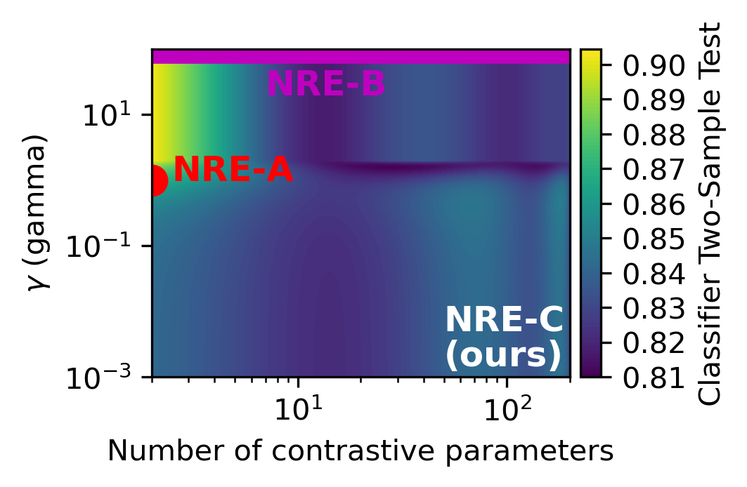
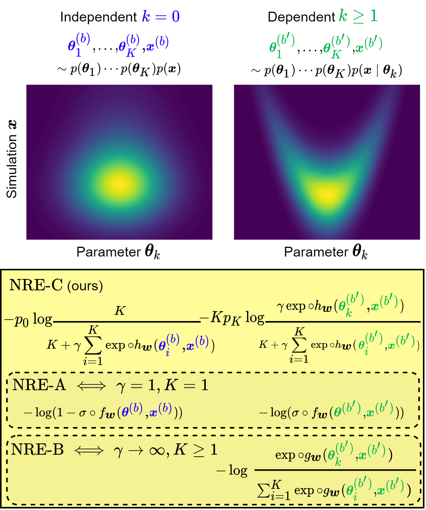
We design a more general formulation of likelihood-to-evidence ratio estimation as a multiclass problem in which the bias inherent to nre-b is discouraged by the loss function and it does not appear at optimum. Figure 1 diagrams the interpolated performance as a function of hyperparameters. It shows which settings recover nre-a and nre-b, also indicating that highest performance occurs with settings distant from these. Figure 2 shows the relationship of the loss functions. We call our framework nre-c and expound the details in Section 2.

An existing importance sampling diagnostic [30] tests whether a classifier can distinguish $p(\boldsymbol{x}\,|\,\boldsymbol{\theta})$ samples from from samples from $p(\boldsymbol{x})$ weighted by the estimated ratio. We demonstrate that, when estimating accurate posteriors, our proposed nre-c passes this diagnostic while nre-b does not.

Taking inspiration from mutual information estimation [58], we propose applying a variational bound on the mutual information between $\boldsymbol{\theta}$ and $\boldsymbol{x}$ in a novel way–as an informative metric measuring a lower bound on the Kullback-Leibler divergence between surrogate posterior estimate $p_{\boldsymbol{w}}(\boldsymbol{\theta}\,|\,\boldsymbol{x})$ and $p(\boldsymbol{\theta}\,|\,\boldsymbol{x})$, averaged over $p(\boldsymbol{x})$. Unlike with two-sample testing methods commonly used in machine learning literature [44], our metric samples only from $p(\boldsymbol{\theta},\boldsymbol{x})$, which is always available in sbi, and does not require samples from the intractable $p(\boldsymbol{\theta}\,|\,\boldsymbol{x})$. Our metric is meaningful to scientists working on problems with intractable posteriors. The technique requires estimating the partition function, which can be expensive. We find the metric to be well correlated with results from two-sample tests.

We evaluate nre-b and nre-c in a fair comparison in several training regimes in Section 3. We perform a hyperparameter search on three simulators with tractable likelihood by benchmarking the behavior when (a) jointly drawn pairs $(\boldsymbol{\theta},\boldsymbol{x})$ are unlimited or when jointly drawn pairs $(\boldsymbol{\theta},\boldsymbol{x})$ are fixed but we (b) can draw from the prior $p(\boldsymbol{\theta})$ without limit or (c) are restricted to the initial pairs. We also perform the sbi benchmark of Lueckmann et al. [44] with our recommended hyperparameters.

2 Methods

The ratio between probability distributions can be estimated using the “likelihood ratio trick” by training a classifier to distinguish samples [27, 66, 19, 12, 69, 50, 30]. We first summarize the loss functions of nre-a and nre-b which approximate the intractable likelihood-to-evidence ratio $r(\boldsymbol{x}\,|\,\boldsymbol{\theta})\coloneqq\frac{p(\boldsymbol{x}\,|\,\boldsymbol{\theta})}{p(\boldsymbol{x})}$. We then elaborate on our proposed generalization, nre-c. Finally, we explain how to recover nre-a and nre-b within our framework and comment on the normalization properties.

nre-a

Hermans et al. [30] train a binary classifier to distinguish $(\boldsymbol{\theta},\boldsymbol{x})$ pairs drawn dependently $p(\boldsymbol{\theta},\boldsymbol{x})$ from those drawn independently $p(\boldsymbol{\theta})p(\boldsymbol{x})$. This classifier is parameterized by a neural network $f_{\boldsymbol{w}}$ which approximates $\log r(\boldsymbol{x}\,|\,\boldsymbol{\theta})$. We seek optimal network weights

$$\boldsymbol{w}^{*}\in\operatorname*{arg\,min}_{\boldsymbol{w}}-\frac{1}{2B}\left[\sum_{b=1}^{B}\log\left(1-\sigma\circ f_{\boldsymbol{w}}(\boldsymbol{\theta}^{(b)},\boldsymbol{x}^{(b)})\right)+\sum_{b^{\prime}=1}^{B}\log\left(\sigma\circ f_{\boldsymbol{w}}(\boldsymbol{\theta}^{(b^{\prime})},\boldsymbol{x}^{(b^{\prime})})\right)\right]$$ (3)

$\boldsymbol{\theta}^{(b)},\boldsymbol{x}^{(b)}\sim p(\boldsymbol{\theta})p(\boldsymbol{x})$ and $\boldsymbol{\theta}^{(b^{\prime})},\boldsymbol{x}^{(b^{\prime})}\sim p(\boldsymbol{\theta},\boldsymbol{x})$ over $B$ samples. nre-a’s ratio estimate converges to $f_{\boldsymbol{w}^{*}}=\log\frac{p(\boldsymbol{x}\,|\,\boldsymbol{\theta})}{p(\boldsymbol{x})}$ given unlimited model flexibility and data. Details can be found in Appendix A.

nre-b

Durkan et al. [16] train a classifier that selects from among $K$ parameters $(\boldsymbol{\theta}_{1},\ldots,\boldsymbol{\theta}_{K})$ which could have generated $\boldsymbol{x}$, in contrast with nre-a’s binary possibilities. One of these parameters $\boldsymbol{\theta}_{k}$ is always drawn jointly with $\boldsymbol{x}$. The classifier is parameterized by a neural network $g_{\boldsymbol{w}}$ which approximates $\log r(\boldsymbol{x}\,|\,\boldsymbol{\theta})$. Training is done over $B$ samples by finding

$$\boldsymbol{w}^{*}\in\operatorname*{arg\,min}_{\boldsymbol{w}}\left[-\frac{1}{B}\sum_{b^{\prime}=1}^{B}\log\frac{\exp\circ g_{\boldsymbol{w}}(\boldsymbol{\theta}_{k}^{(b^{\prime})},\boldsymbol{x}^{(b^{\prime})})}{\sum_{i=1}^{K}\exp\circ g_{\boldsymbol{w}}(\boldsymbol{\theta}_{i}^{(b^{\prime})},\boldsymbol{x}^{(b^{\prime})})}\right]$$ (4)

where $\boldsymbol{\theta}_{1}^{(b^{\prime})},\ldots,\boldsymbol{\theta}_{K}^{(b^{\prime})}\sim p(\boldsymbol{\theta})$ and $\boldsymbol{x}^{(b^{\prime})}\sim p(\boldsymbol{x}\,|\,\boldsymbol{\theta}_{k}^{(b^{\prime})})$. Given unlimited model flexibility and data nre-b’s ratio estimate converges to ${g_{\boldsymbol{w}^{*}}(\boldsymbol{\theta},\boldsymbol{x})=\log\frac{p(\boldsymbol{\theta}\,|\,\boldsymbol{x})}{p(\boldsymbol{\theta})}+c_{\boldsymbol{w}^{*}}(\boldsymbol{x})}$. Details are in Appendix A.

2.1 Contrastive Neural Ratio Estimation

Our proposed algorithm nre-c trains a classifier to identify which $\boldsymbol{\theta}$ among $K$ candidates is responsible for generating a given $\boldsymbol{x}$, inspired by nre-b. We added another option that indicates $\boldsymbol{x}$ was drawn independently, inspired by nre-a. The introduction of the additional class yields a ratio without the specific $c_{\boldsymbol{w}}(\boldsymbol{x})$ bias at optimum. Define $\boldsymbol{\Theta}\coloneqq(\boldsymbol{\theta}_{1},...,\boldsymbol{\theta}_{K})$ and conditional probability

$$p_{\textsc{nre-c}}(\boldsymbol{\Theta},\boldsymbol{x}\,|\,y=k)\coloneqq\begin{cases}p(\boldsymbol{\theta}_{1})\cdots p(\boldsymbol{\theta}_{K})p(\boldsymbol{x})&k=0\\ p(\boldsymbol{\theta}_{1})\cdots p(\boldsymbol{\theta}_{K})p(\boldsymbol{x}\,|\,\boldsymbol{\theta}_{k})&k=1,\ldots,K\end{cases}.$$ (5)

We set marginal probabilities $p(y=k)\coloneqq p_{K}$ for all $k\geq 1$ and ${p(y=0)\coloneqq p_{0}}$, yielding the relationship $p_{0}=1-Kp_{K}$. Let the odds of any pair being drawn dependently to completely independently be $\gamma\coloneqq\frac{Kp_{K}}{p_{0}}$. We now use Bayes’ formula to compute the conditional probability

$$p(y=k\,|\,\boldsymbol{\Theta},\boldsymbol{x}) =\frac{p(y=k)\,p(\boldsymbol{\Theta},\boldsymbol{x}\,|\,y=k)/p(\boldsymbol{\Theta},\boldsymbol{x}\,|\,y=0)}{\sum_{i=0}^{K}p(y=i)\,p(\boldsymbol{\Theta},\boldsymbol{x}\,|\,y=i)/p(\boldsymbol{\Theta},\boldsymbol{x}\,|\,y=0)}$$ (6)

$$=\frac{p(y=k)\,p(\boldsymbol{\Theta},\boldsymbol{x}\,|\,y=k)/p(\boldsymbol{\Theta},\boldsymbol{x}\,|\,y=0)}{p(y=0)+\sum_{i=1}^{K}p(y=i)\,p(\boldsymbol{\Theta},\boldsymbol{x}\,|\,y=i)/p(\boldsymbol{\Theta},\boldsymbol{x}\,|\,y=0)}$$

$$=\begin{cases}\frac{K}{K+\gamma\sum_{i=1}^{K}r(\boldsymbol{x}\,|\,\boldsymbol{\theta}_{i})}&k=0\\ \frac{\gamma\,r(\boldsymbol{x}\,|\,\boldsymbol{\theta}_{k})}{K+\gamma\sum_{i=1}^{K}r(\boldsymbol{x}\,|\,\boldsymbol{\theta}_{i})}&k=1,\ldots,K\end{cases}.$$

We dropped the nre-c subscript and substituted in $\gamma$ to replace the $p(y)$ class probabilities. We train a classifier, parameterized by neural network $h_{\boldsymbol{w}}(\boldsymbol{\theta},\boldsymbol{x})$ with weights $\boldsymbol{w}$, to approximate (6) by

$$q_{\boldsymbol{w}}(y=k\,|\,\boldsymbol{\Theta},\boldsymbol{x})=\begin{cases}\frac{K}{K+\gamma\sum_{i=1}^{K}\exp\circ h_{\boldsymbol{w}}(\boldsymbol{\theta}_{i},\boldsymbol{x})}&k=0\\ \frac{\gamma\,\exp\circ h_{\boldsymbol{w}}(\boldsymbol{\theta}_{k},\boldsymbol{x}))}{K+\gamma\sum_{i=1}^{K}\exp\circ h_{\boldsymbol{w}}(\boldsymbol{\theta}_{i},\boldsymbol{x})}&k=1,\ldots,K.\end{cases}.$$ (7)

We note that (7) still satisfies $\sum_{k=0}^{K}q_{\boldsymbol{w}}(y=k\,|\,\boldsymbol{\Theta},\boldsymbol{x})=1$, no matter the parameterization.

Optimization

We design a loss function that encourages $h_{\boldsymbol{w}}(\boldsymbol{\theta},\boldsymbol{x})=\log\frac{p(\boldsymbol{x}\,|\,\boldsymbol{\theta})}{p(\boldsymbol{x})}$ at convergence, and holds at optimum with unlimited flexibility and data. We introduce the cross entropy loss

$$\ell(\boldsymbol{w}) \coloneqq\mathbb{E}_{p(y,\boldsymbol{\Theta},\boldsymbol{x})}\left[-\log q_{\boldsymbol{w}}(y\,|\,\boldsymbol{\Theta},\boldsymbol{x})\right]$$ (8)

$$=-p_{0}\mathbb{E}_{p(\boldsymbol{\Theta},\boldsymbol{x}\,|\,y=0)}\left[\log q_{\boldsymbol{w}}(y=0\,|\,\boldsymbol{\Theta},\boldsymbol{x})\right]-p_{K}\sum_{k=1}^{K}\mathbb{E}_{p(\boldsymbol{\Theta},\boldsymbol{x}\,|\,y=k)}\left[\log q_{\boldsymbol{w}}(y=k\,|\,\boldsymbol{\Theta},\boldsymbol{x})\right]$$

$$=-p_{0}\mathbb{E}_{p(\boldsymbol{\Theta},\boldsymbol{x}\,|\,y=0)}\left[\log q_{\boldsymbol{w}}(y=0\,|\,\boldsymbol{\Theta},\boldsymbol{x})\right]-Kp_{K}\mathbb{E}_{p(\boldsymbol{\Theta},\boldsymbol{x}\,|\,y=K)}\left[\log q_{\boldsymbol{w}}(y=K\,|\,\boldsymbol{\Theta},\boldsymbol{x})\right]$$

and minimize it towards $\boldsymbol{w}^{*}\in\operatorname*{arg\,min}_{\boldsymbol{w}}\ell(\boldsymbol{w})$. We point out that the final term is symmetric up to permutation of $\boldsymbol{\Theta}$, enabling the replacement of the sum by multiplication with $K$. When $\gamma$ and $K$ are known, $p_{0}=\frac{1}{1+\gamma}$ and $p_{K}=\frac{1}{K}\frac{\gamma}{1+\gamma}$ under our constraints. Without loss of generality, we let $\boldsymbol{\theta}_{1},\ldots,\boldsymbol{\theta}_{K}\sim p(\boldsymbol{\theta})$ and $\boldsymbol{x}\sim p(\boldsymbol{x}\,|\,\boldsymbol{\theta}_{K})$. An empirical estimate of the loss on $B$ samples is therefore

$$\hat{\ell}_{\gamma,K}(\boldsymbol{w}) \coloneqq-\frac{1}{B}\Bigg{[}\frac{1}{1+\gamma}\sum_{b=1}^{B}\log q_{\boldsymbol{w}}\left(y=0\,|\,\boldsymbol{\Theta}^{(b)},\boldsymbol{x}^{(b)}\right)$$ (9)

$$\phantom{\approx-\frac{1}{B}\Bigg{[}}+\frac{\gamma}{1+\gamma}\sum_{b^{\prime}=1}^{B}\log q_{\boldsymbol{w}}\left(y=K\,|\,\boldsymbol{\Theta}^{(b^{\prime})},\boldsymbol{x}^{(b^{\prime})}\right)\Bigg{]}.$$

In the first term, the classifier sees a completely independently drawn sample of $\boldsymbol{x}$ and $\boldsymbol{\Theta}$ while $\boldsymbol{\theta}_{K}$ is drawn jointly with $\boldsymbol{x}$ in the second term. In both terms, the classifier considers $K$ choices. In practice, we bootstrap both $\boldsymbol{\theta}_{1}^{(b)},\ldots,\boldsymbol{\theta}_{K}^{(b)}$ and $\boldsymbol{\theta}_{1}^{(b^{\prime})},\ldots,\boldsymbol{\theta}_{K-1}^{(b^{\prime})}$ from the same mini-batch and compare them to the same $\boldsymbol{x}$, similarly to nre-a and nre-b. Proof of the above is in Appendix B.

Recovering nre-a and nre-b

nre-c is general because specific hyperparameter settings recover nre-a and nre-b. To recover nre-a one should set $\gamma=1$ and $K=1$ in (9) yielding

$$\hat{\ell}_{1,1}(\boldsymbol{w}) =-\frac{1}{2B}\Bigg{[}\sum_{b=1}^{B}\log\frac{1}{1+\exp\circ h_{\boldsymbol{w}}(\boldsymbol{\theta}^{(b)},\boldsymbol{x}^{(b)})}+\sum_{b^{\prime}=1}^{B}\log\frac{\exp\circ h_{\boldsymbol{w}}(\boldsymbol{\theta}^{(b^{\prime})},\boldsymbol{x}^{(b^{\prime})})}{1+\exp\circ h_{\boldsymbol{w}}(\boldsymbol{\theta}^{(b^{\prime})},\boldsymbol{x}^{(b^{\prime})})}\Bigg{]}$$ (10)

$$=-\frac{1}{2B}\left[-\sum_{b=1}^{B}\log\left(1-\sigma\circ h_{\boldsymbol{w}}(\boldsymbol{\theta}^{(b)},\boldsymbol{x}^{(b)})\right)+\sum_{b^{\prime}=1}^{B}\log\left(\sigma\circ h_{\boldsymbol{w}}(\boldsymbol{\theta}^{(b^{\prime})},\boldsymbol{x}^{(b^{\prime})})\right)\right]$$

where we dropped the lower index. Recovering nre-b requires taking the limit $\gamma\to\infty$ in the loss function. In that case, the first term goes to zero, and second term converges to the softmax function.

$$\hat{\ell}_{\infty,K}(\boldsymbol{w}) =\lim_{\gamma\to\infty}\hat{\ell}_{\gamma,K}(\boldsymbol{w}) =-\frac{1}{B}\Bigg{[}\sum_{b^{\prime}=1}^{B}\log\frac{\exp\circ h_{\boldsymbol{w}}(\boldsymbol{\theta}_{k},\boldsymbol{x}))}{\sum_{i=1}^{K}\exp\circ h_{\boldsymbol{w}}(\boldsymbol{\theta}_{i},\boldsymbol{x})}\Bigg{]}$$ (11)

is determined by substitution into (9). Both equations are obviously the same as their counterparts.

Estimating a normalized posterior

In the limit of infinite data and infinite neural network capacity (width, depth) the optimal classifier trained using nre-c (with $\gamma\in\mathbb{R}^{+}$) satisfies the equality:

$$h_{\boldsymbol{w}^{*}}(\boldsymbol{\theta},\boldsymbol{x}) =\log\frac{p(\boldsymbol{\theta}\,|\,\boldsymbol{x})}{p(\boldsymbol{\theta})}.$$ (12)

In particular, we have that the following normalizing constant is trivial:

$$Z(\boldsymbol{x}) :=\int\exp\left(h_{\boldsymbol{w}^{*}}(\boldsymbol{\theta},\boldsymbol{x})\right)p(\boldsymbol{\theta})\,d\boldsymbol{\theta}=\int p(\boldsymbol{\theta}\,|\,\boldsymbol{x})\,d\boldsymbol{\theta}=1.$$ (13)

This is a result of Lemma 1 in Appendix B. However, practitioners never operate in this setting, rather they use finite sample sizes and neural networks with limited capacity that are optimized locally. The non-optimal function $\exp(h_{\boldsymbol{w}}(\boldsymbol{\theta},\boldsymbol{x}))$ does not have a direct interpretation as a ratio of probability distributions, rather as the function to weigh the prior $p(\boldsymbol{\theta})$ to approximate the unnormalized posterior. In other words, we find the following approximation for the posterior $p(\boldsymbol{\theta}\,|\,\boldsymbol{x})$:

$$p_{\boldsymbol{w}}(\boldsymbol{\theta}\,|\,\boldsymbol{x}) :=\frac{\exp(h_{\boldsymbol{w}}(\boldsymbol{\theta},\boldsymbol{x}))}{Z_{\boldsymbol{w}}(\boldsymbol{x})}p(\boldsymbol{\theta}), Z_{\boldsymbol{w}}(\boldsymbol{x}) :=\int\exp\left(h_{\boldsymbol{w}}(\boldsymbol{\theta},\boldsymbol{x})\right)p(\boldsymbol{\theta})\,d\boldsymbol{\theta},$$ (14)

where in general the normalizing constant is not trivial, i.e. $Z_{\boldsymbol{w}}(\boldsymbol{x})\neq 1$. As stated above, the nre-c (and nre-a) objective encourages $Z_{\boldsymbol{w}}(\boldsymbol{x})$ to converge to $1$. This is in sharp contrast to nre-b, where even at optimum with an unrestricted function class a non-trivial $\boldsymbol{x}$-dependent bias term can appear.

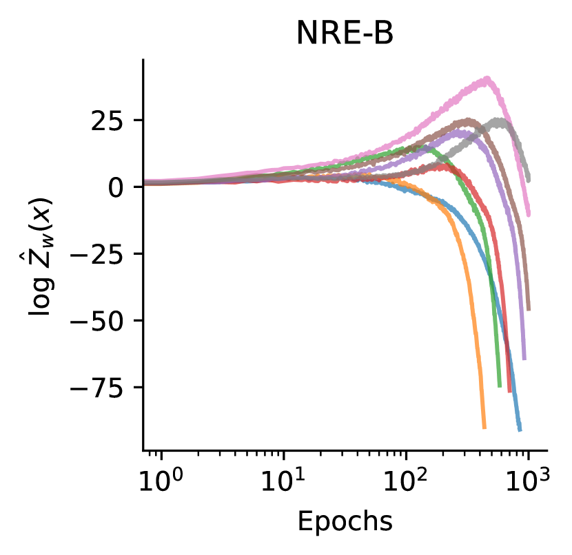
There is no restriction on how pathological the nre-b bias $c_{\boldsymbol{w}}(\boldsymbol{x})$ can be. Consider a minimizer of (4), the nre-b loss function, $h_{\boldsymbol{w}^{\ast}}+c_{\boldsymbol{w}^{\ast}}(\boldsymbol{x})$. Adding any function $d(\boldsymbol{x})$ cancels out in the fraction and is also a minimizer of (4). This freedom complicates any numerical computation of the normalizing constant and renders the importance sampling diagnostic from Section 2.2 generally inapplicable. We report Monte Carlo estimates of $Z_{\boldsymbol{w}}(\boldsymbol{x})$ on a test problem across hyperparameters in Figure 14.

2.2 Measuring performance & ratio estimator diagnostics

sbi is difficult to verify because, for many use cases, the practitioner cannot compare surrogate $p_{\boldsymbol{w}}(\boldsymbol{\theta}\,|\,\boldsymbol{x})$ to the intractable ground truth $p(\boldsymbol{\theta}\,|\,\boldsymbol{x})$. Incongruous with the practical use case for sbi, much of the literature has focused on measuring the similarity between surrogate and posterior using two-samples tests on tractable problems. For comparison with literature, we first reference a two-sample exactness metric which requires a tractable posterior. We then discuss diagnostics which do not require samples from $p(\boldsymbol{\theta}\,|\,\boldsymbol{x})$, commenting on the relevance for each nre algorithm with empirical results. Further, we find that a known variational bound to the mutual information is tractable to estimate within sbi, that it bounds the average Kullback-Leibler divergence between surrogate and posterior, and propose to use it for model comparison on intractable inference tasks.

Comparing to a tractable posterior with estimates of exactness

Assessments of approximate posterior quality are available when samples can be drawn from both the posterior $\boldsymbol{\theta}\sim p(\boldsymbol{\theta}\,|\,\boldsymbol{x})$ and the approximation $\boldsymbol{\theta}\sim q(\boldsymbol{\theta}\,|\,\boldsymbol{x})$. In the deep learning-based sbi literature, exactness is measured as a function of computational cost, usually simulator calls. We investigate this with nre-c in Section 3.3.

Based on the recommendations of Lueckmann et al. [44] our experimental results are measured using the Classifier Two-Sample Test (C2ST) [17, 40, 41]. A classifier is trained to distinguish samples from either the surrogate or the ground truth posterior. An average classification probability on holdout data of 1.0 implies that samples from each distribution are easily identified; 0.5 implies either the distributions are the same or the classifier does not have the capacity to distinguish them.

Importance sampling diagnostic

(a) Posteriors

(b) Likelihood and reweighted marginal generative models.

(c) Receiver operating characteristic.

Figure 3: The figures visualize the importance sampling diagnostic on ratio estimators trained using nre-b and nre-c. (a) Both methods produce satisfactory posterior estimates that agree with $p(\boldsymbol{\theta}\,|\,\boldsymbol{x})$. (b) $p(\boldsymbol{x}\,|\,\boldsymbol{\theta})$ is shown along with $p(\boldsymbol{x})$ samples weighted by nre-a $\exp\circ f_{\boldsymbol{w}}(\boldsymbol{\theta},\boldsymbol{x})$ and nre-b $\exp\circ g_{\boldsymbol{w}}(\boldsymbol{\theta},\boldsymbol{x})$. Each plot corresponds to a different $\boldsymbol{\theta}$. Despite high posterior accuracy, the nre-b estimates are distinct from $p(\boldsymbol{x}\,|\,\boldsymbol{\theta})$. (c) Two classifier’s roc curves, each trained to distinguish $p(\boldsymbol{x}\,|\,\boldsymbol{\theta})$ samples from $p(\boldsymbol{x})$ samples weighted by the corresponding nre’s $\hat{r}$ estimate. The classifier failed to distinguish likelihood samples from the nre-c weighted data samples, but successfully identified nre-b weighted samples. nre-b accurately approximates the posterior, but fails the diagnostic. nre-c produces an accurate posterior surrogate and passes the diagnostic.

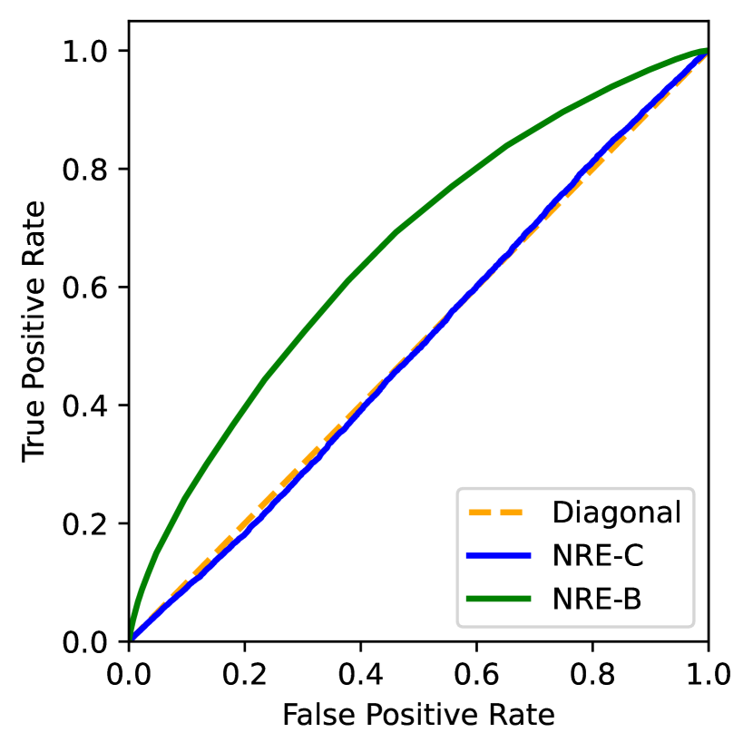
An accurate likelihood-to-evidence weight transforms the data distribution into the likelihood by ${p(\boldsymbol{x}\,|\,\boldsymbol{\theta})=p(\boldsymbol{x})r(\boldsymbol{x}\,|\,\boldsymbol{\theta})}$. Since nre necessitates simulator access, we can test the ratio estimator by training a classifier to distinguish unweighted $p(\boldsymbol{x}\,|\,\boldsymbol{\theta})$ samples from weighted $p(\boldsymbol{x})\hat{r}(\boldsymbol{x}\,|\,\boldsymbol{\theta})$ samples, where $\hat{r}$ implies an estimate. Indistinguishability between samples implies either that the approximate ratio is accurate for parameter $\boldsymbol{\theta}$ or that the classifier does not have sufficient power to find predictive features. Issues with classification power can be detected by assessing the classifier’s ability to distinguish $p(\boldsymbol{x})$ from $p(\boldsymbol{x}\,|\,\boldsymbol{\theta})$. The performance can be visualized in a receiver operating curve (roc) or measured by the area under the curve (roc auc). This diagnostic has been used for ratio estimators before [12, 30] but it comes from training models under covariate shift [62]. It is particularly appealing because it does not require samples from $p(\boldsymbol{\theta}\,|\,\boldsymbol{x})$.

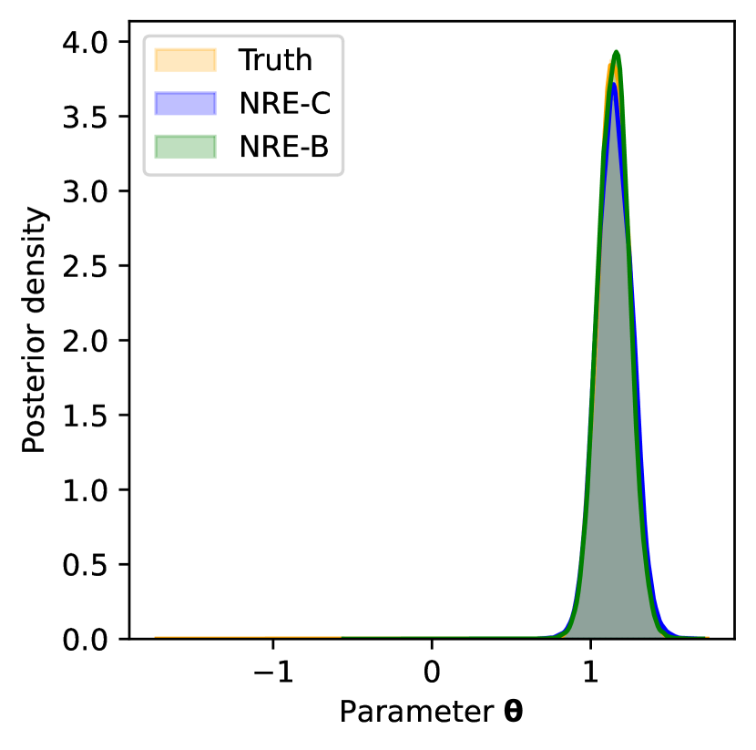
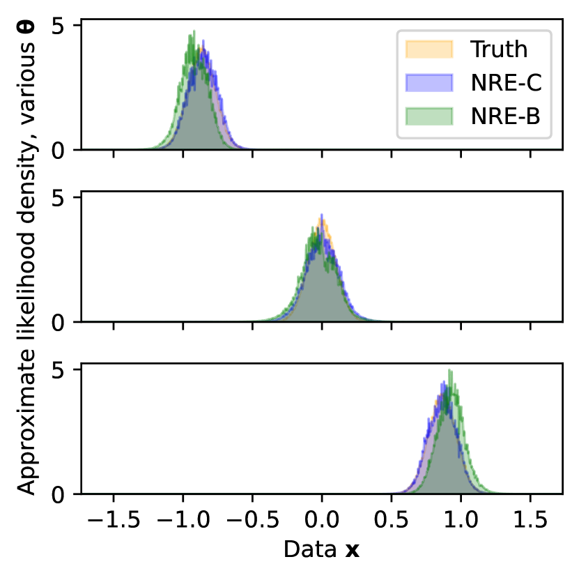
Durkan et al. [16] do not mention this diagnostic in their paper, but due to its intrinsic bias nre-b does not fulfill the identity necessary for this diagnostic to hold at optimum. The unknown factor that depends on $\boldsymbol{x}$ implies ${p(\boldsymbol{x}\,|\,\boldsymbol{\theta})\neq p(\boldsymbol{x})\exp\circ g_{\boldsymbol{w}}(\boldsymbol{x}\,|\,\boldsymbol{\theta})}$. We provide empirical evidence of this issue in Figure 3. Although nre-b accurately approximates the true posterior, it demonstrably fails the diagnostic. Given the limited options for verification of sbi results, this presents a major problem by significantly limiting the trustworthiness of nre-b on any problem with an intractable posterior. In Appendix B, we show that the unrestricted nre-b-specific $c_{\boldsymbol{w}}(\boldsymbol{x})$ bias means approximating $p(\boldsymbol{x}\,|\,\boldsymbol{\theta})$ with normalized importance weights will not solve the issue.

Mutual information bound

Selecting the surrogate model most-similar to the target posterior remains intractable without access to $p(\boldsymbol{\theta}\,|\,\boldsymbol{x}_{o})$. Nevertheless, practitioners must decide which surrogate should approximate the posterior across training and hyperparameter search. Unfortunately, the validation losses between different versions of nre and different $K$ and $\gamma$ settings are not comparable. A good heuristic is to choose the model which minimizes the Kullback-Leibler divergence on average over possible data $p(\boldsymbol{x})$. In Appendix D, we prove the relationship between $I(\boldsymbol{\theta};\boldsymbol{x})$, the mutual information with respect to $p(\boldsymbol{\theta},\boldsymbol{x})$, our models’ variational bound $I_{\boldsymbol{w}}^{(0)}(\boldsymbol{\theta};\boldsymbol{x})$, and the average kld

$$\mathbb{E}_{p(\boldsymbol{x})}\left[\textsc{kld}(p(\boldsymbol{\theta}\,|\,\boldsymbol{x})\,\|\,p_{\boldsymbol{w}}(\boldsymbol{\theta}\,|\,\boldsymbol{x}))\right]=I(\boldsymbol{\theta};\boldsymbol{x})-I_{\boldsymbol{w}}^{(0)}(\boldsymbol{\theta};\boldsymbol{x}),$$ (15)

$$I_{\boldsymbol{w}}^{(0)}(\boldsymbol{\theta};\boldsymbol{x})\coloneqq\mathbb{E}_{p(\boldsymbol{\theta},\boldsymbol{x})}\left[\log\hat{r}(\boldsymbol{x}\,|\,\boldsymbol{\theta})\right]-\mathbb{E}_{p(\boldsymbol{x})}\left[\log\mathbb{E}_{p(\boldsymbol{\theta})}[\hat{r}(\boldsymbol{x}\,|\,\boldsymbol{\theta})]\right].$$ (16)

The non-negativity of all terms in (15) implies $I(\boldsymbol{\theta};\boldsymbol{x})\geq I_{\boldsymbol{w}}^{(0)}(\boldsymbol{\theta};\boldsymbol{x})$; that means the model which minimizes $-I_{\boldsymbol{w}}^{(0)}(\boldsymbol{\theta};\boldsymbol{x})$ best satisfies our heuristic. We propose to approximate $-I_{\boldsymbol{w}}^{(0)}(\boldsymbol{\theta};\boldsymbol{x})$ with Monte Carlo using held-out data as a metric for model selection during training and across hyperparameters. The expectation values average over $p(\boldsymbol{\theta},\boldsymbol{x})$, $p(\boldsymbol{\theta})$, and $p(\boldsymbol{x})$. We can sample from all of these distributions in the sbi context. Since the second term in (16) computes the average log partition function, our metric can compare nre-b-based surrogates to nre-c-based ones. However, the metric comes with the normal challenges of estimating the log partition function, which can be very expensive. Additionally, the presence of the ratio in the integrand can make this integral high variance. We treat a generally tractable bound in Appendix D. We go into much more depth there and discuss of the relevance to Neural Posterior Estimation [53, 42, 21, 16]. While the application to sbi is novel, bounds on the mutual information have been broadly investigated for contrastive representation learning and mutual information estimation [22, 23, 25, 4, 71, 58].

Empirical expected coverage probability

For a candidate distribution to qualify as the posterior, integrating over data must return the prior. A measurement that follows from calibration to the prior is called expected coverage probability. Expected coverage probability can be estimated with samples from $p(\boldsymbol{\theta},\boldsymbol{x})$ and any amortized sbi method. Although important, ability to compute this metric does not distinguish nre-c. We refer the interested reader to Hermans et al. [31]. We note that popular sequential techniques generally render this diagnostic inapplicable, with exceptions [47, 48, 10].

3 Experiments

We perform experiments in three settings to measure the exactness of surrogate models under various hyperparameters and training regimes. Section 3.1 aims to identify whether data or architecture is the bottleneck in accuracy by drawing from the joint with every mini-batch. The next experiments aim to determine how to optimally extract inference information given a limited amount of simulation data. Section 3.2 leverages a cheap prior by drawing new contrastive parameters with every mini-batch. Finally, Section 3.3 applies the commonplace training regime for deep learning-based sbi literature of fixed data and bootstrapped contrastive parameters. In this setting, we also benchmark nre-c on ten inference tasks from Lueckmann et al. [44] using our recommended hyperparameters.

On all hyperparameter searches we consider three simulators from the simulation-based inference benchmark, namely SLCP, Two Moons, and Gaussian Mixture [44]. SLCP is a difficult inference task which has a simple likelihood and complex posterior [21, 56]. Parameters are five dimensional and the data are four samples from a two dimensional random variable. Two Moons is two dimensional with a crescent-shaped bimodal posterior. Finally, the Gaussian Mixture data draws from a mixture of two, two-dimensional normal distributions with extremely different covariances [64, 3, 70, 63].

Our surrogate models are parameterized by one of these architectures: Small NN is like the benchmark with 50 hidden units and two residual blocks. Large NN has 128 hidden units and three residual blocks. We use batch normalization, unlike the benchmark. We compare their performance on a grid of $\gamma$ and $K$ values. We report post-training results using the C2ST, and mid-training validation loss for insight into convergence rate. We generally use residual networks [28] with batch normalization [33] and train them using adam [37]. We also run nre-b with the same architecture for comparison. To compare with nre-b we set the number of total contrastive parameters equal.

What does fair comparison mean in our experimentation? We compare models across fixed number of gradient steps. This implies that models with more classes, i.e., greater $K$, evaluate the classifier-in-training on more pairs at a given training step than a model with fewer classes. An alternative which we do not apply in this paper: Vary the number of gradient steps, holding the number of pair evaluations fixed, i.e., a model with higher $K$ sees the same number of pairs as a model with lower $K$ but the model with lower $K$ has been updated more times. We leave this analysis for future work.

3.1 Behavior with unlimited data

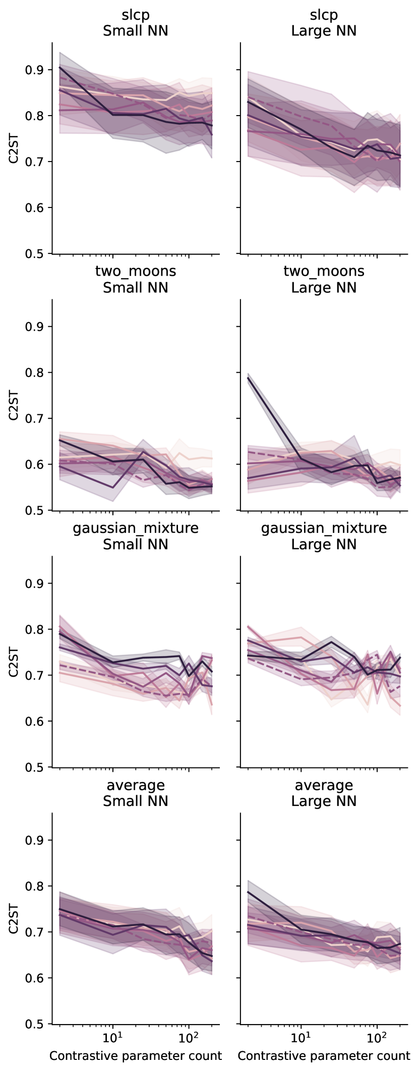
What is responsible for inaccuracies of the surrogate model when training has saturated? (a) the amount of training data (b) the flexibility of the model? In this section we provide new simulation and parameter data with every mini-batch and train until saturation, thereby eliminating the possibility of (a). The newly drawn mini-batch parameters $\boldsymbol{\Theta}$ are bootstrapped for the contrastive pairs.

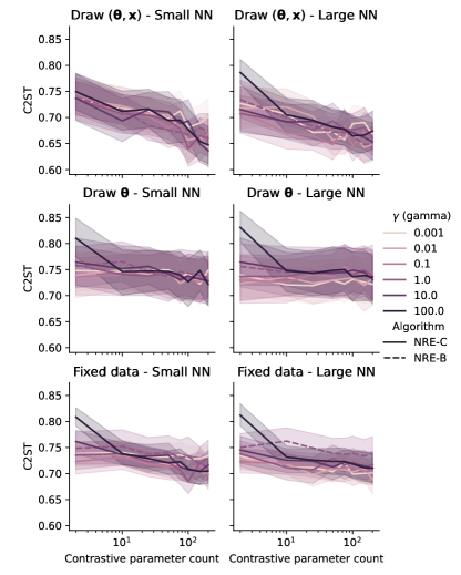
The setting is similar to rej-abc where simulations are drawn until the posterior has converged. The results of this study will provide a baseline to compare with limited-data results and help us understand how the deep learning architecture’s limitations are affected by our introduced hyperparameters. The results are reported in the top row of Figure 5.

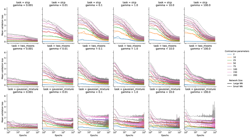
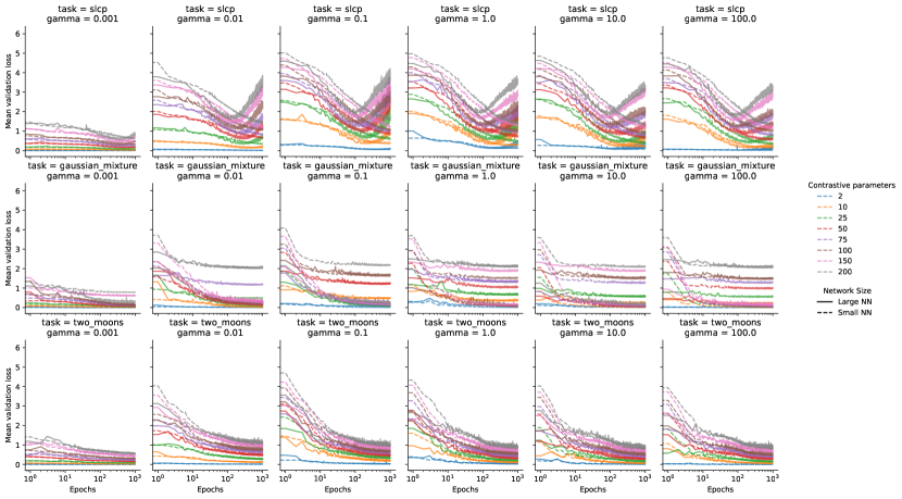
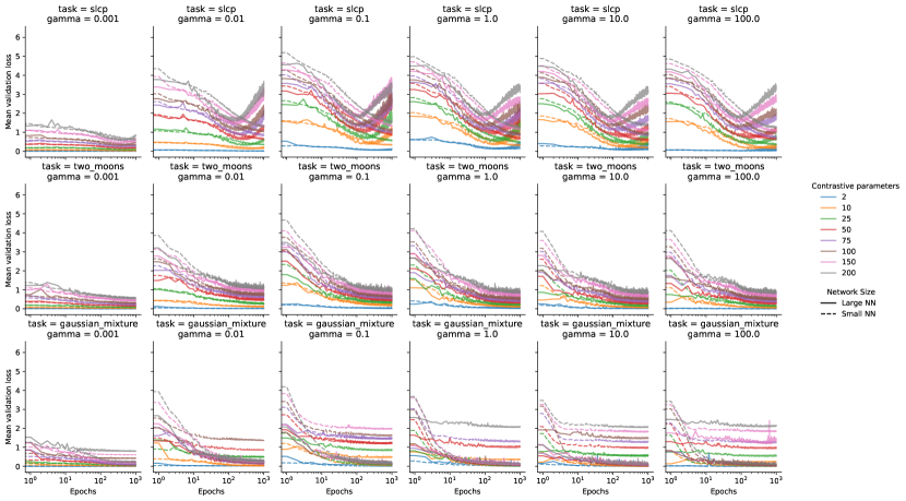
The trend is that increasing the number of contrastive examples helps nre-b and nre-c. There is not a clear trend with respect to $\gamma$ in the C2ST. Study of the detailed validation losses in Appendix C reveals that high $\gamma$ is associated with higher variance validation loss during training, but here it does not seem to strongly affect convergence rate. Saturation is reached before the maximum number of epochs have elapsed and Large NN converges to a better result. Although obfuscated in the averaged results in Figure 5, the result is obvious on SLCP, the most difficult inference task that provides an opportunity for a more flexible architecture to improve.

We argue that generally the performance bottleneck has to do with the number of contrastive parameters, network flexibility, or training details rather than the amount of data. Despite saturating validation losses, the C2ST improves based on these factors. Intuitively a more flexible model could continue to extract information from this unlimited set of jointly drawn $(\boldsymbol{\theta},\boldsymbol{x})$ pairs. This has some consequence because network flexibility may limit performance in the benchmark case. Appendix C contains more detailed results.

3.2 Leveraging fast priors (drawing theta)

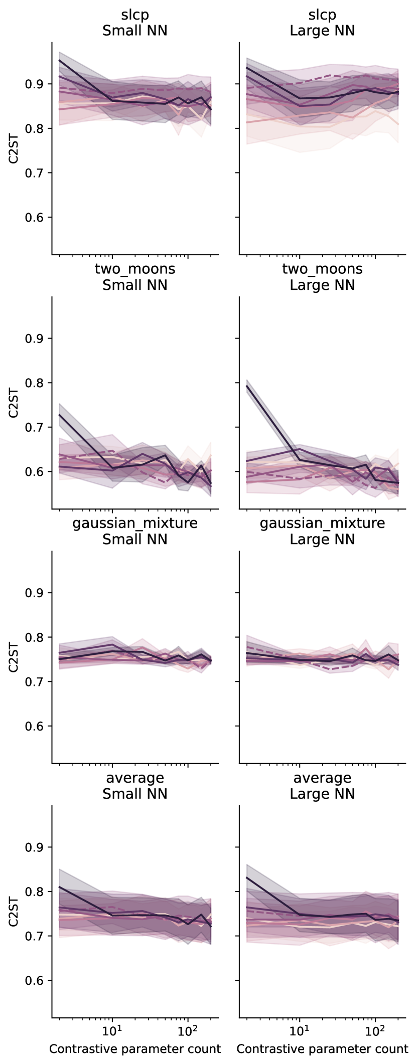
In practice, the simulator is often slow but one can often draw from the prior at the same pace as training a neural network for one mini-batch. Our goal is to understand how our hyperparameter are affected by this setting and whether it is valuable to use this technique in practice. To our knowledge, this training regime has not been explored in the deep learning-based sbi literature.

Initially we draw a fixed set of around 20,000 samples $(\boldsymbol{\theta},\boldsymbol{x})\sim p(\boldsymbol{\theta},\boldsymbol{x})$. For every mini-batch during training, we sample all necessary contrastive parameters from the prior. For each term in $\hat{\ell}_{\gamma,K}$ we take the same batch of contrastive parameters and reshuffle them, thereby equalizing the number of samples seen by nre-b and nre-c, up to bootstrap. The averaged C2ST results from the three inference tasks are reported in the middle row of Figure 5.

The resulting estimators are markedly less sensitive to the number of contrastive parameters than in Section 3.1. The number of network parameters has a positive effect, although again this is best seen on the hardest task, SLCP, in the Appendix C. Empirically, lower values of $\gamma$ improve performance with Large NN; however, there is still high variance and this result may be from noise. In this setting, $\gamma\neq 1$ has a very small negative effect on convergence rate compared to unity, as seen in the validation loss plots in Appendix C. Since training has saturated, we claim this result implies drawing contrastive parameters from the prior helps extract the maximum amount of information from fixed simulation data $\boldsymbol{x}$–without being strongly affected by the number of contrastive parameters $K$.

(a) nre-b

(b) nre-c

Figure 4: Our proposed metric, a negative bound on the mutual information $-\hat{I}_{\boldsymbol{w}}^{(0)}(\boldsymbol{\theta};\boldsymbol{x})$, for the SLCP task estimated over the validation set versus training epochs using (a) nre-b and (b) nre-c with various values of $\gamma$ and $K$, a Large NN architecture, and fixed training data. The bound permits visualization of the convergence rates and pairwise comparison across models. When $K$ is fixed, small $\gamma$ slows convergences but leads to better optima than large $\gamma$. When $\gamma$ is fixed, small $K$ slows convergence but leads to better optima than high $K$. Unlike when computing the validation loss directly, this metric does not exhibit a $\gamma$ and $K$ dependent bias as seen in Figures 7, 8, and 9.

3.3 Simulation-based inference benchmark

In this section, we assume the traditional literature setting of limited simulation and prior budget. Once we’ve selected hyperparameters based on a grid search of a subset of the sbi benchmark, we perform the entire benchmark with those hyperparameters.

Figure 5: Exactness of nre posterior surrogates is computed for various contrastive parameter counts, $\gamma$ values, and architectures on an average of three tasks from the sbi benchmark [44]. C2ST assigns 1.0 to inaccurate and 0.5 to accurate posterior approximation. (top) $p(\boldsymbol{\theta},\boldsymbol{x})$ was sampled at every mini-batch during training. The accuracy strongly depends on $K$. (mid) A fixed number of dependent $(\boldsymbol{\theta},\boldsymbol{x})$ pairs were drawn, but $p(\boldsymbol{\theta})$ was sampled at every mini-batch during training. In this regime, $K$ has a smaller effect. (bot) The training data is completely fixed. Contrastive parameters are drawn in a bootstrap from the mini-batch. On the problems with fixed simulation data $\boldsymbol{x}$, higher $K$ improves accuracy and small $\gamma$ with larger architectures slightly improves performance. The effects of the architecture are more clearly seen on difficult problems like SLCP in Appendix C.

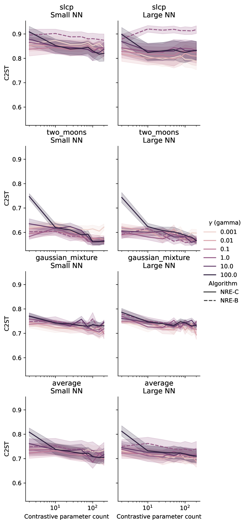
Hyperparameter search

To compare to the previous two sections, the amount of training data was fixed such that each epoch was comparable to Section 3.1, this amounts to about 20,000 samples. We first inspect the C2ST results in the last row of Figure 5. The sensitivity to $K$ appears less than in Section 3.1 but more than in Section 3.2. Smaller $\gamma$ slightly improves Large NN’s performance but the noise makes this result uncertain. The larger network performs better, see Appendix C.

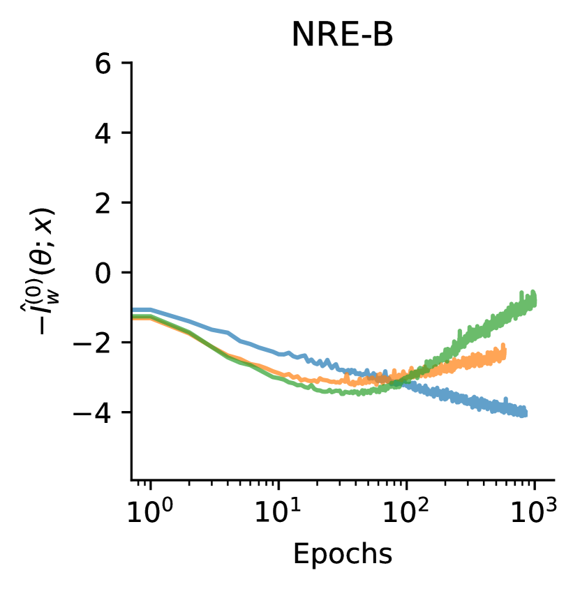
We do a Monte Carlo estimate of our proposed metric, denoted $-\hat{I}_{\boldsymbol{w}}^{(0)}(\boldsymbol{\theta};\boldsymbol{x})$, to show performance on the SLCP task as a function of epochs in Figure 4. For both nre-b and nre-c, increasing $K$ tends to positively affect the convergence rate. Generally, with fixed $\gamma$ and high $K$, peak performance is negatively impacted, in contrast to results from Figure 5 using the C2ST. Generally, with fixed $K$, small $\gamma$ slows convergences but leads to better optima than large $\gamma$. When $\gamma$ is fixed, small $K$ slows convergence but leads to better optima than high $K$. See Figure 12.

Our take-away is that $\gamma\in[0.1,10]$ has a small effect, otherwise learning can become unstable or very slow. $\gamma=1$ has a good compromise on high convergence rate without sacrificing too much performance. Generally, we saw improved performance on the C2ST by increasing contrastive parameters $K$. However, larger $K$ also increases the magnitude of the normalizing constant, and extreme values reduced the performance on $-\hat{I}_{\boldsymbol{w}}^{(0)}(\boldsymbol{\theta};\boldsymbol{x})$, see Appendix D. Since the benchmark compares C2ST, we optimized our architecture based on that metric. Due to bootstrapping parameters from the batched $\boldsymbol{\theta}$, the maximum $K$ is $B/2$ without reusing any $\boldsymbol{\theta}$ to compare with $\boldsymbol{x}$. This is considering both terms in our loss function.

Benchmark

We performed the benchmark tasks from Lueckmann et al. [44] with nre-c. Our architecture and hyperparameters deviate based on the results of the last paragraph. We applied the largest number of computationally practical contrastive parameters, namely $K=99$, and set $\gamma=1$. Since we identified potential architecture bottlenecks in Sections 3.1 and 3.3, we used Large NN for our results. The averaged results are visible in Table 1. Sequential estimates are prepended with an s, all other estimates are amortized. We trained a five amortized estimators per task with five seeds, then we predicted the posterior for each of the ten observations $\boldsymbol{x}_{1},\ldots,\boldsymbol{x}_{10}$. Lueckmann et al. [44] trained an estimator for every $\boldsymbol{x}$ with a new seed. The reported C2ST for our method is averaged across ten posteriors per seed with five seeds, i.e., fifty C2ST computations per task. The other methods are averaged across one posterior per seed with ten seeds, i.e., ten C2ST computations per task.

nre-c performed better than nre-b at all budgets and generally well among the amortized algorithms. The high performance at $10^{5}$ simulation budget implies that our design has high capacity and may scale well. Sequential methods naturally lead to high exactness since they are tailored to the specific observation $\boldsymbol{x}_{o}$, but they come with drawbacks since they cannot practically perform empirical expected coverage tests [31, 48] nor bound the mutual information, as discussed in Section 2.2. Detailed results per task can be found in Appendix C.

Table 1: Averaged C2ST for various budgets on the simulation-based inference benchmark [44]. An s implies a sequential i.e. non-amortized method.

	C2ST
Simulation budget	$10^{3}$	$10^{4}$	$10^{5}$
Algorithm
nre-c (ours)	0.853	0.762	0.680
rej-abc	0.965	0.920	0.871
nle	0.826	0.753	0.723
npe	0.838	0.736	0.654
nre (nre-b)	0.867	0.811	0.762
smc-abc	0.948	0.873	0.816
snle	0.783	0.704	0.655
snpe	0.796	0.677	0.615
snre (snre-b)	0.788	0.703	0.610

4 Conclusion

We introduced a generalization of nre-a and nre-b which discourages the nre-b specific $c_{\boldsymbol{w}}(\boldsymbol{x})$ bias term and produces an unbiased estimate of the likelihood-to-evidence ratio at optimum. This property has implications for the importance sampling diagnostic, which is critical to practitioners. We suggested using a variational bound on the mutual information as a model-selection metric that could replace the C2ST averaged over several observations. It is significantly more practical since it does not require access to the ground truth posterior; however, it remains a lower bound so we don’t know the overall quality of our estimator. Further discussions and derivations related to the mutual information are available in Appendix D.

In the context of nre-c, we found that increasing the number of contrastive parameters $K$ improved the C2ST in most cases, at the price of increasing the normalizing constant. Setting $\gamma\approx 1$ was generally the fastest to saturate and lower values seemed to slightly improve performance with the Large NN and fixed simulation data. These results indicate that better performance can be achieved by using nre-c with these hyperparameters than the other version of nre. When both training parameters $\boldsymbol{\theta}$ and simulation data $\boldsymbol{x}$ are unlimited, the architecture size plays an important role in the quality of surrogate model. We tried drawing contrastive parameters from the prior, a commonly available practical use-case, and found that it damped the effect of $K$ on the C2ST. According to the C2ST, for highest accuracy with a fixed budget set $K$ large, up to the mini-batch size divided by 2, and $\gamma\approx 1.0$ for the best convergence rate. When the prior is sampled for every mini-batch, applying a higher $K$ may be less valuable. In situations where the normalizing constant should be very close to unity, i.e., for practitioners who want to run diagnostics, drawing $\boldsymbol{\theta}$ from the prior with every mini-batch and using a smaller $K$ and $\gamma$ is best.

Broader Impact

The societal implications of sbi are similar to other inference methods. The methods are primarily scientific and generally lead to interesting discoveries; however, one must be careful to use an accurate generative model and to carefully test empirical results. Model mismatch and untested inference can lead to incorrect conclusions. That is why we emphasize the importance of the diagnostics in our paper. This nuance can be missed by practitioners doing inference in any field; however, special care should be taken when producing inference results that may be used for making decisions in areas like predicting hidden variables that describe human behavior or determining what factors are responsible for climate change. This list is non-comprehensive and not specific to sbi.

Checklist

The checklist follows the references. Please read the checklist guidelines carefully for information on how to answer these questions. For each question, change the default [TODO] to [Yes] , [No] , or [N/A] . You are strongly encouraged to include a justification to your answer, either by referencing the appropriate section of your paper or providing a brief inline description. For example:

• Did you include the license to the code and datasets? [Yes] See Section .

• Did you include the license to the code and datasets? [No] The code and the data are proprietary.

• Did you include the license to the code and datasets? [N/A]

Please do not modify the questions and only use the provided macros for your answers. Note that the Checklist section does not count towards the page limit. In your paper, please delete this instructions block and only keep the Checklist section heading above along with the questions/answers below.

1. For all authors…

   1. Do the main claims made in the abstract and introduction accurately reflect the paper’s contributions and scope? [Yes] We introduce the generalization in Section 2.1. We show that it has the properties we claim in Appendix B. We perform the experiments in Section 3 and make a hyperparameter recommendation in Section 4

   2. Did you describe the limitations of your work? [Yes] We discussed the behavior of ours and other algorithms in the finite sample setting, see Section 2.1 and limitations of existing to test the convergence of our method, see Section 2.2.

   3. Did you discuss any potential negative societal impacts of your work? [Yes] We briefly mentioned them in Section 4.

   4. Have you read the ethics review guidelines and ensured that your paper conforms to them? [Yes] This work applies toy simulation data thus no ethics concerns were raised by the paper. Other matters of ethics during experimentation and writing conformed.

2. If you are including theoretical results…

   1. Did you state the full set of assumptions of all theoretical results? [Yes] These are laid out in Appendix B.

   2. Did you include complete proofs of all theoretical results? [Yes] We have only one real theoretical result and that is proven in Lemma 1. Anything else follows algebraically and is shown in detail.

3. If you ran experiments…

   1. Did you include the code, data, and instructions needed to reproduce the main experimental results (either in the supplemental material or as a URL)? [Yes] The code will be made available via a link in the supplemental material. It is a python package with example calls and self-explanatory installation instructions. The details will be shown in Section C. Results will be released upon acceptance.

   2. Did you specify all the training details (e.g., data splits, hyperparameters, how they were chosen)? [Yes] Additionally to the hyperparameter search which is the primary experimental result, seen in Section 3, we included more details in Appendix C.

   3. Did you report error bars (e.g., with respect to the random seed after running experiments multiple times)? [Yes] The hyperparameter searches indeed included error bars in Section 3. We did not include error bars in the computation of the diagnostic since we emphasize that it is made possible by our method, not its statistical properties. The details of the benchmark, including some uncertainty in the last experimental section are shown in Appendix C.

   4. Did you include the total amount of compute and the type of resources used (e.g., type of GPUs, internal cluster, or cloud provider)? [Yes] This is discussed in Appendix C.

4. If you are using existing assets (e.g., code, data, models) or curating/releasing new assets…

   1. If your work uses existing assets, did you cite the creators? [Yes] We cited the benchmark [44] several times in the paper. Also the sbi package [68]

   2. Did you mention the license of the assets? [Yes] The license is mentioned in Appendix A

   3. Did you include any new assets either in the supplemental material or as a URL? [Yes] I will link to my code in the supplemental material as discussed above. Upon acceptance results will be made available.

   4. Did you discuss whether and how consent was obtained from people whose data you’re using/curating? [N/A] The publicly available data was used in accordance with the aforementioned license in [44]. There was no need to get consent or mention it in the paper.

   5. Did you discuss whether the data you are using/curating contains personally identifiable information or offensive content? [N/A] The data is generated by toy mathematical models which abstractly relate parameters to data. It is highly unlikely any culture would find them offensive.

5. If you used crowdsourcing or conducted research with human subjects…

   1. Did you include the full text of instructions given to participants and screenshots, if applicable? [N/A]

   2. Did you describe any potential participant risks, with links to Institutional Review Board (IRB) approvals, if applicable? [N/A]

   3. Did you include the estimated hourly wage paid to participants and the total amount spent on participant compensation? [N/A]

Appendix A Relationship to other sbi methods

Sampling in sbi

All nre (and sbi) algorithms require samples from the joint distribution $p(\boldsymbol{\theta},\boldsymbol{x})$. nre additionally requires samples from the product of marginals $p(\boldsymbol{\theta})p(\boldsymbol{x})$. Sampling the joint with a simulator requires drawing from the prior $\boldsymbol{\theta}\sim p(\boldsymbol{\theta})$ then passing that parameter into the simulator to produce $\boldsymbol{x}\sim p(\boldsymbol{x}\,|\,\boldsymbol{\theta})$. Sampling the product of marginals is simple, just take another sample from the prior $\boldsymbol{\theta}^{\prime}\sim p(\boldsymbol{\theta})$ and pair it with our simulation from before. Then we have $(\boldsymbol{\theta},\boldsymbol{x})\sim p(\boldsymbol{\theta},\boldsymbol{x})$ and $(\boldsymbol{\theta}^{\prime},\boldsymbol{x})\sim p(\boldsymbol{\theta})p(\boldsymbol{x})$. In practice, we refer to this operation as a bootstrap within a mini-batch where we take $\boldsymbol{\theta}^{\prime}$ from other parameter-simulation pairs and reuse them to create samples drawn from the product of marginals $p(\boldsymbol{\theta})p(\boldsymbol{x})$. nre-c sometimes requires more $\boldsymbol{\theta}$ samples, often represented as $\boldsymbol{\Theta}$. These can be generated by merely concatenating several samples from $p(\boldsymbol{\theta})$. Some sbi methods, e.g., sequential methods, sometimes replace the prior with a proposal distribution $\tilde{p}(\boldsymbol{\theta})$.

Amortized and sequential sbi

Recently, significant progress has been made in sbi, especially with so-called sequential methods that use active learning to draw samples from the posterior for a fixed observation-of-interest $\boldsymbol{x}_{o}$ [24, 53, 69, 42, 20, 56, 21, 59, 16, 63, 61, 35, 60, 18]. Amortized sbi algorithms, that can draw samples from the posterior for arbitrary observation $\boldsymbol{x}$, have also enjoyed attentive development [9, 30, 36, 8, 47, 48]. Hermans et al. [31] and Miller et al. [48] argue that their intrinsic empirical testability makes amortized methods better applicable to the scientific use-case despite their inherently higher training expense. The last pillar of development has been into assessment methods that determine the reliability of approximate inference results. In the machine learning community, the focus has been on evaluating the exactness of estimates for tractable problems [44]. Evaluation methods which apply in the practical case where no tractable posterior is available are under development [12, 7, 67, 14, 29]. We make a contribution to this effort in Appendix D.

Contrastive learning, nre-b, and npe

We call our method Contrastive Neural Ratio Estimation because it the classifier is trained to identify which pairs of $\boldsymbol{\theta}$ and $\boldsymbol{x}$ should be paired together. Gutmann et al. [25] created an overview of contrastive learning for statistical problems generally. Specific connections are in the loss functions with nre-a closely corresponding to noise-contrastive estimation (NCE) [22, 23] and nre-b with RankingNCE, InfoNCE, and related [46, 45, 49, 71].

A core aspect of our paper focus on the effects of the nre-b ratio estimate biased by $c_{\boldsymbol{w}}(\boldsymbol{x})$ at optimum. Ma and Collins [45] also investigate the effects on the partition function when applying a binary or multi-class loss variant for estimating conditional energy-based models. Due to the similarity in the loss functions, they exhibit a similar bias in their partition function. In order to correct this bias they estimate $c_{\boldsymbol{w}}(\boldsymbol{x})$ directly. We did not attempt to do this for our problem, so we do not have intuition about the effectiveness of such an approach to the likelihood-based diagnostic in nre. Although, since $c_{\boldsymbol{w}}(\boldsymbol{x})$ is completely unconstrained, it may be quite difficult to estimate. We believe that this would be an alternative direction for future work.

Durkan et al. [16] emphasize the connection between nre and contrastive learning in their paper which created a framework such that Neural Posterior Estimation (npe) and nre-b can be trained using the same loss function. The addition of an independently drawn $(\boldsymbol{\Theta},\boldsymbol{x})$ set means that the nre-c framework is not trivially applicable for computing the normalizing constant on atoms necessary for their sequential version of npe.

Software

Our experiments used sbi [68], which is released under an AGPL-3.0 license, and sbibm [44], which is released under an MIT license. They implement various neural sbi algorithms and benchmark problems respectively.

A.1 Full derivation of other nre methods using our framework

Here we present a derivation of the previous works nre-a [30] and nre-b [30] in our framwork.

nre-a

To estimate $r(\boldsymbol{x}\,|\,\boldsymbol{\theta})$, Hermans et al. [30] introduce an indicator variable $y$ which switches between dependently and independently drawn samples. We have conditional probability

$$p_{\textsc{nre-a}}(\boldsymbol{\theta},\boldsymbol{x}\,|\,y=k)=\begin{cases}p(\boldsymbol{\theta})p(\boldsymbol{x})&k=0\\ p(\boldsymbol{\theta},\boldsymbol{x})&k=1\end{cases}.$$ (17)

Each class’ marginal probability is set equally, $p(y=0)=p(y=1)$. Dropping the nre-a subscript, the probability that $(\boldsymbol{\theta},\boldsymbol{x})$ was drawn jointly is encoded in the another conditional probability

$$p(y=1\,|\,\boldsymbol{\theta},\boldsymbol{x}) =\frac{p(\boldsymbol{\theta},\boldsymbol{x}\,|\,y=1)p(y=1)}{p(\boldsymbol{\theta},\boldsymbol{x}\,|\,y=1)p(y=1)+p(\boldsymbol{\theta},\boldsymbol{x}\,|\,y=0)p(y=0)}$$ (18)

$$=\frac{p(\boldsymbol{\theta},\boldsymbol{x})}{p(\boldsymbol{\theta},\boldsymbol{x})+p(\boldsymbol{\theta})p(\boldsymbol{x})}=\frac{r(\boldsymbol{x}\,|\,\boldsymbol{\theta})}{1+r(\boldsymbol{x}\,|\,\boldsymbol{\theta})}.$$

nre-a estimates $\log\hat{r}(\boldsymbol{x}\,|\,\boldsymbol{\theta})$ with neural network $f_{\boldsymbol{w}}$ with weights $\boldsymbol{w}$. Training is done by minimizing the binary cross-entropy of $q_{\boldsymbol{w}}(y=1\,|\,\boldsymbol{\theta},\boldsymbol{x})\coloneqq\sigma\circ f_{\boldsymbol{w}}(\boldsymbol{\theta},\boldsymbol{x})$ relative to $p(y,\boldsymbol{\theta},\boldsymbol{x})$. For $B$ samples,

$$\boldsymbol{w}=\operatorname*{arg\,min}_{\boldsymbol{w}}\left[-\frac{1}{B}\sum_{b=1}^{B}\log\left(1-\sigma\circ f_{\boldsymbol{w}}(\boldsymbol{\theta}^{(b)},\boldsymbol{x}^{(b)})\right)-\frac{1}{B}\sum_{b^{\prime}=1}^{B}\log\left(\sigma\circ f_{\boldsymbol{w}}(\boldsymbol{\theta}^{(b^{\prime})},\boldsymbol{x}^{(b^{\prime})})\right)\right]$$ (19)

where $\boldsymbol{\theta}^{(b)},\boldsymbol{x}^{(b)}\sim p(\boldsymbol{\theta})p(\boldsymbol{x})$ and $\boldsymbol{\theta}^{(b^{\prime})},\boldsymbol{x}^{(b^{\prime})}\sim p(\boldsymbol{\theta},\boldsymbol{x})$. In practice, $\boldsymbol{\theta}^{(b^{\prime})}$ is bootstrapped from within the mini-batch to produce $\boldsymbol{\theta}^{(b)}$. nre-a’s ratio estimate converges to ${f_{\boldsymbol{w}}=\log\frac{p(\boldsymbol{x}\,|\,\boldsymbol{\theta})}{p(\boldsymbol{x})}=\log r(\boldsymbol{x}\,|\,\boldsymbol{\theta})}$ given unlimited model flexibility and data

nre-b

Durkan et al. [16] estimate $r(\boldsymbol{x}\,|\,\boldsymbol{\theta})$ by training a classifier that selects from among $K$ parameters $\boldsymbol{\Theta}\coloneqq(\boldsymbol{\theta}_{1},\ldots,\boldsymbol{\theta}_{K})$ which could have generated $\boldsymbol{x}$. In contrast with nre-a, one of these parameters $\boldsymbol{\theta}_{k}$ is always drawn jointly with $\boldsymbol{x}$. Let $y$ be a random variable which indicates which one of $K$ parameters simulated $\boldsymbol{x}$. The marginal probability $p(y=k)\coloneqq 1/K$ is uniform. That means

$$p_{\textsc{nre-b}}(\boldsymbol{\Theta},\boldsymbol{x}\,|\,y=k)\coloneqq p(\boldsymbol{\theta}_{1})\cdots p(\boldsymbol{\theta}_{K})p(\boldsymbol{x}\,|\,\boldsymbol{\theta}_{k})$$ (20)

defines our conditional probability for parameters and data. Bayes’ rule reveals a conditional distribution over $y$, dropping the nre-b subscript, therefore

$$p(y=k\,|\,\boldsymbol{\Theta},\boldsymbol{x})=\frac{p(\boldsymbol{\Theta},\boldsymbol{x}\,|\,y=k)p(y=k)}{p(\boldsymbol{\Theta},\boldsymbol{x})}=\frac{p(\boldsymbol{\Theta},\boldsymbol{x}\,|\,y=k)p(y=k)}{\sum_{i}p(\boldsymbol{\Theta},\boldsymbol{x}\,|\,y=i)p(y=i)}\\ =\frac{p(\boldsymbol{\theta}_{1})\cdots p(\boldsymbol{\theta}_{k},\boldsymbol{x})\cdots p(\boldsymbol{\theta}_{K})}{\sum_{i}p(\boldsymbol{\theta}_{1})\cdots p(\boldsymbol{\theta}_{i},\boldsymbol{x})\cdots p(\boldsymbol{\theta}_{K})}=\frac{p(\boldsymbol{\theta}_{k}\,|\,\boldsymbol{x})/p(\boldsymbol{\theta}_{k})}{\sum_{i}p(\boldsymbol{\theta}_{i}\,|\,\boldsymbol{x})/p(\boldsymbol{\theta}_{i})}=\frac{r(\boldsymbol{x}\,|\,\boldsymbol{\theta}_{k})}{\sum_{i}r(\boldsymbol{x}\,|\,\boldsymbol{\theta}_{i})}.$$ (21)

nre-b estimates $\log\hat{r}(\boldsymbol{x}\,|\,\boldsymbol{\theta})$ with a neural network $g_{\boldsymbol{w}}$. Training is done by minimizing the cross entropy of $q_{\boldsymbol{w}}(y=k\,|\,\boldsymbol{\Theta},\boldsymbol{x})\coloneqq\exp\circ g_{\boldsymbol{w}}(\boldsymbol{\theta}_{k},\boldsymbol{x})/\sum_{i}\exp\circ g_{\boldsymbol{w}}(\boldsymbol{\theta}_{i},\boldsymbol{x})$ relative to $p(y,\boldsymbol{x},\boldsymbol{\theta})$;

$$\boldsymbol{w}=\operatorname*{arg\,min}_{\boldsymbol{w}}\mathbb{E}_{p(y,\boldsymbol{\Theta},\boldsymbol{x})}\left[-q_{\boldsymbol{w}}(y\,|\,\boldsymbol{\Theta},\boldsymbol{x})\right]\approx\operatorname*{arg\,min}_{\boldsymbol{w}}\left[-\frac{1}{B}\sum_{b^{\prime}=1}^{B}\log\frac{\exp\circ g_{\boldsymbol{w}}(\boldsymbol{\theta}_{k}^{(b^{\prime})},\boldsymbol{x}^{(b^{\prime})})}{\sum_{i}\exp\circ g_{\boldsymbol{w}}(\boldsymbol{\theta}_{i}^{(b^{\prime})},\boldsymbol{x}^{(b^{\prime})})}\right]$$ (22)

where $\boldsymbol{\theta}_{1}^{(b^{\prime})},\ldots,\boldsymbol{\theta}_{K}^{(b^{\prime})}\sim p(\boldsymbol{\theta})$, $k^{(b^{\prime})}\sim p(y)$, and $\boldsymbol{x}^{(b^{\prime})}\sim p(\boldsymbol{x}\,|\,\boldsymbol{\theta}_{k}^{(b^{\prime})})$ over $B$ samples. In our parameterization and given unlimited flexibility and data, ${g_{\boldsymbol{w}}(\boldsymbol{\theta},\boldsymbol{x})=\log\frac{p(\boldsymbol{\theta}\,|\,\boldsymbol{x})}{p(\boldsymbol{\theta})}+c_{\boldsymbol{w}}(\boldsymbol{x})}$ at convergence. The extra term enters because the optimal classifier for (22) need not be normalized.

Appendix B Theoretical Arguments

We present first the proof of convergence for nre-c. Afterwards, we discuss the properties of estimated importance weights in nre-b.

B.1 Proof of convergence of nre-c

Lemma 1.

Consider for $k=0,\dots,K$ the following probability distributions for $\boldsymbol{z}$:

$$p(\boldsymbol{z}\,|\,y=k).$$ (23)

and $p(y)>0$ a probability distribution for $y$. Put $p_{k}:=p(y=k)$ for $k=1,\dots,K$. For functions $f_{k}:\,\mathcal{Z}\to\mathbb{R}$, $k=1,\dots,K$, let:

$$q(y=k\,|\,f,\boldsymbol{z}):=\begin{cases}\frac{1}{1+\sum_{j=1}^{K}\frac{p_{j}}{p_{0}}\exp(f_{j}(\boldsymbol{z}))},&k=0,\\ \frac{\frac{p_{k}}{p_{0}}\exp(f_{k}(\boldsymbol{z}))}{1+\sum_{j=1}^{K}\frac{p_{j}}{p_{0}}\exp(f_{j}(\boldsymbol{z}))},&k=1,\dots,K.\end{cases}$$ (24)

Note that $q(y=k\,|\,f,\boldsymbol{z})>0$ for all $k=0,\dots,K$ and that $\sum_{k=0}^{K}q(y=k\,|\,f,\boldsymbol{z})=1$ for every $K$-tuple $f=(f_{k})_{k=1,\dots,K}$ and $\boldsymbol{z}\in\mathcal{Z}$. Consider a minimizer:

$$f^{*} \in\operatorname*{arg\,min}_{f}\mathbb{E}_{p(\boldsymbol{z}\,|\,y)p(y)}\left[-\log q(y\,|\,f,\boldsymbol{z})\right].$$ (25)

Then we have for $p(\boldsymbol{z})$-almost-all $\boldsymbol{z}$ and all $k=1,\dots,K$:

$$f^{*}_{k}(\boldsymbol{z}) =\log\frac{p(\boldsymbol{z}|y=k)}{p(\boldsymbol{z}|y=0)}.$$ (26)

Proof.

We have:

$$f^{*} \in\operatorname*{arg\,min}_{f}\mathbb{E}_{p(\boldsymbol{z}\,|\,y)p(y)}\left[-\log q(y\,|\,f,\boldsymbol{z})\right]$$ (27)

$$=\operatorname*{arg\,min}_{f}\mathbb{E}_{p(\boldsymbol{z},y)}\left[\log\frac{p(y\,|\,\boldsymbol{z})}{q(y\,|\,f,\boldsymbol{z})}\right]$$ (28)

$$=\operatorname*{arg\,min}_{f}\mathbb{E}_{p(\boldsymbol{z})}\left[\textsc{kld}(p(y\,|\,\boldsymbol{z})\|q(y\,|\,f,\boldsymbol{z}))\right],$$ (29)

which is minimized, when $\textsc{kld}=0$, thus:

$$0 =\textsc{kld}(p(y\,|\,\boldsymbol{z})\|q(y\,|\,f^{*},\boldsymbol{z})),$$ (30)

which implies that for $p(\boldsymbol{z})$-almost-all $\boldsymbol{z}$:

$$q(y\,|\,f^{*},\boldsymbol{z}) =p(y\,|\,\boldsymbol{z})=\frac{p(\boldsymbol{z}|y)}{p(\boldsymbol{z})}p(y).$$ (31)

So we get with the definition of $q(y\,|\,f^{*},\boldsymbol{z})$:

$$\frac{p(\boldsymbol{z}|y=0)}{p(\boldsymbol{z})}p_{0} =\frac{1}{1+\sum_{j=1}^{K}\frac{p_{j}}{p_{0}}\exp(f^{*}_{j}(\boldsymbol{z}))}, k=0,$$ (32)

$$\frac{p(\boldsymbol{z}|y=k)}{p(\boldsymbol{z})}p_{k} =\frac{\frac{p_{k}}{p_{0}}\exp(f^{*}_{k}(\boldsymbol{z}))}{1+\sum_{j=1}^{K}\frac{p_{j}}{p_{0}}\exp(f^{*}_{j}(\boldsymbol{z}))}, k=1,\dots,K.$$ (33)

Dividing the latter by the former gives for $k=1,\dots,K$:

$$\frac{p(\boldsymbol{z}|y=k)}{p(\boldsymbol{z}|y=0)}\frac{p_{k}}{p_{0}} =\frac{p_{k}}{p_{0}}\exp(f^{*}_{k}(\boldsymbol{z})),$$ (34)

implying for $k=1,\dots,K$ and $p(\boldsymbol{z})$-almost-all $\boldsymbol{z}$:

$$f_{k}^{*}(\boldsymbol{z}) =\log\frac{p(\boldsymbol{z}|y=k)}{p(\boldsymbol{z}|y=0)}.$$ (35)

This shows the claim. ∎

We used the symbol kld to imply the Kullback-Leibler Divergence. The proof in Lemma 1 is slightly more general than necessary for our typical case. All our functions $f_{k}$ are typically the same, namely the evaluation of a neural network with weights $\boldsymbol{w}$. Rather than searching for the function $f$ which minimizes the objective, we search for the weights, but these are equivalent. Finally to make everything fit, we set $\boldsymbol{z}\coloneqq(\boldsymbol{\theta},\boldsymbol{x})$.

B.2 Properties of the importance sampling diagnostic on biased ratio estimates

In Section 2.2 we discuss the importance sampling diagnostic, in which the estimated ratio is tested by comparing weighted samples from $\boldsymbol{x}\sim p(\boldsymbol{x})$ to unweighted samples from $\boldsymbol{x}\sim p(\boldsymbol{x}\,|\,\boldsymbol{\theta})$. The estimated ratio from nre-c is merely $\exp(h_{\boldsymbol{w}}(\boldsymbol{\theta},\boldsymbol{x}))$ and is therefore not restricted to have the properties of a ratio of probability distributions, except at optimum with unlimited flexibility and data. The importance sampling diagnostic is designed to test whether the estimated ratio is close to having these properties for a fixed $\boldsymbol{\theta}$. One way to improve ratios estimated by nre-c is to compute the normalizing constant $Z_{\boldsymbol{w}}(\boldsymbol{x})$, which should be close to one, and replace the ratio with this “normalized” version.

The unrestricted nature of the nre-b-specific $c_{\boldsymbol{w}}(\boldsymbol{x})$ bias means that the normalization constant $Z_{\boldsymbol{w}}(\boldsymbol{x})$ does not have to be close to one. Further, we show that the unrestricted bias means that the normalizing constant for two nre-b ratio estimators, which are equivalent in terms of their loss function (22), is not unique, i.e., the estimate is ill-posed. This property means that normalizing nre-b will not, in general, produce an estimator which passes the diagnostic.

Consider two ratio estimates with the relationship $\hat{r}_{1}(\boldsymbol{x}\,|\,\boldsymbol{\theta})=\hat{r}_{2}(\boldsymbol{x}\,|\,\boldsymbol{\theta})/C(\boldsymbol{x})$ where $C$ is an positive function of $\boldsymbol{x}$ resulting from the aggregation of the exponentiated bias. Given $N$ samples $\boldsymbol{x}_{n}\sim p(\boldsymbol{x})$ with weights $w_{1}(\boldsymbol{x}_{n})=\hat{r}_{1}(\boldsymbol{x}_{n}\,|\,\boldsymbol{\theta})$ and $w_{2}(\boldsymbol{x}_{n})=\hat{r}_{2}(\boldsymbol{x}_{n}\,|\,\boldsymbol{\theta})$, we can compute the importance-normalized weights by

$$\bar{w}_{1}(\boldsymbol{x}_{n}) =\frac{w_{1}(\boldsymbol{x}_{n})}{\sum_{i=1}^{N}w_{1}(\boldsymbol{x}_{i})}, \bar{w}_{2}(\boldsymbol{x}_{n}) =\frac{w_{2}(\boldsymbol{x}_{n})}{\sum_{i=1}^{N}w_{2}(\boldsymbol{x}_{i})}.$$ (36)

However, if we substitute this constant back into our expression, we find that the weights do not agree

$$\bar{w}_{1}(\boldsymbol{x}_{n})=\frac{w_{2}(\boldsymbol{x}_{n})/C(\boldsymbol{x}_{n})}{\sum_{i=1}^{N}w_{2}(\boldsymbol{x}_{i})/C(\boldsymbol{x}_{i})} \neq\bar{w}_{2}(\boldsymbol{x}_{n}).$$ (37)

Therefore, normalization does not “protect” against scaling bias introduced by a function in $\boldsymbol{x}$. nre-b does not penalize functional biases like $C(\boldsymbol{x})$, so even ratios considered optimal by nre-b can easily fail the diagnostic. Meanwhile, nre-c encourages terms like $C(\boldsymbol{x})$ towards one. That has the effect of making the $C(\boldsymbol{x})\approx 1$ drop out of the normalized importance weights, thus making performance on the diagnostic indicative of a better ratio estimate, given enough classifier flexibility.

Appendix C Experimental Details

Computational costs

Our experiments were performed on a cluster of Nvidia Titan V graphics processing units. The primary expense was the hyperparameter search within Sections 3.1, 3.2, and the first part of Section 3.3. The run of those experiments took about 50,000 gpu-minutes total considering all of our current data. Since there were several iterations, we multiply this by three to estimate total compute. The next expense was the computation of sbibm in Section 3.3 that took about 24,000 gpu-minutes. Together these equal about 2880 gpu-hours. An estimate for the total carbon contributions corresponds to 311.04 kgCO₂. Luckily, our clusters run completely on wind power offsetting the contribution. Estimations were conducted using the MachineLearning Impact calculator presented in [39].

Architecture and training

The centerpiece of our method is the neural network $h_{\boldsymbol{w}}$ which is trained as a classifier. The hyperparameter choices here were fairly constant throughout the experiments. Any hyperparameters for training or architecture which were consistent across experiments are listed in Table 2. Hidden features and number of resnet blocks depend on the architecture. Large NN uses three resnet blocks with 128 features, while Small NN uses two resnet blocks and 50 features.

Table 2: Architecture

Hyperparameter	Value
Activation Function	relu
amsgrad	No
Architecture	resnet
Batch normalization	Yes
Batch size	1024
Dropout	No
Max epochs	1000
Learning rate	0.0005
Optimizer	adam
Weight Decay	0.0
Standard-score Observations	Using first batch
Standard-score Parameters	Using first batch

C.1 Hyperparameter search measured with C2ST

In this section, we trained many neural networks with different hyperparameter settings on three different tasks from Lueckmann et al. [44]. We trained both architectures, Large and Small NN, on a grid of $\gamma$ and $K$ values with nre-b and nre-c. No matter whether we were training with unlimited draws from the joint, prior, or fixed data we designed an epoch such that it has 20 training mini-batches and 2 validation mini-batches. For fixed initial data and prior this corresponds to a simulation budget of 22,528. The mean validation losses per-epoch for these networks is visible in Figures 7, 8, and 9.

For one specific problem, we also computed validation loss at a fixed $\gamma$ and $K$ no matter the training regime in an effort to produce comparable validation losses, specifically $\gamma=1$ and $K=1$ aka the nre-a regime. This training setting reverses some of the trends we’ve seen when validated on the same loss as training data. We did not apply it further since this could bias results. See Figure 11. To compare, we also plot the validation loss on the sample problem but using the $\gamma$ and $K$ each model was trained with. See Figure 10, note that the bias depending on $\gamma$ and $K$ is clearly visible (just as in the other validation loss plots).

Once the networks were trained, we drew samples from ten per-task posteriors based on ten predefined observations $\boldsymbol{x}_{i}$ with $i\in 1,2,\ldots,10$. This leveraged the amortized property of nre-c. Samples were drawn on these problems using rejection sampling. Once the samples were drawn, they were compared to ground truth posterior samples from the benchmark with the C2ST. The detailed plot which shows per-task behavior is available in Figure 6.

(a) Draw $(\boldsymbol{\theta},\boldsymbol{x})$.

(b) Draw $\boldsymbol{\theta}$.

(c) Fixed data.

Figure 6: A measure of exactness comparing to the ground truth to the samples from a surrogate posterior, the C2ST, is plotted as a function of number of contrastive parameters. Each row corresponds to a different task: SLCP, Two Moons, Gaussian Mixture, and an average of the results across tasks. Both nre-c and nre-b are shown along with various $\gamma$ values, and architectures are shown. Recall that C2ST assigns 1.0 to inaccurate and 0.5 to accurate approximations. (a) Corresponds to Section 3.1 where unlimited draws from the joint are allowed. (b) Corresponds to Section 3.2 where unlimited draws from the prior are allowed but the $\boldsymbol{x}$ data is fixed. (c) Corresponds to Section 3.3 where both the initial draws of $\boldsymbol{\theta}$ and $\boldsymbol{x}$ are the only data available.

Figure 7: The validation loss from nre-c is reported versus epochs on various tasks, $\gamma$, $K$, and architectures trained using unlimited draws from the joint distribution. The rows correspond to different tasks, columns to different $\gamma$, colors to different $K$, and dashed or solid lines to Small and Large NN respectively. These plots correspond with the technique discussed in Section 3.1.

Figure 8: The validation loss from nre-c is reported versus epochs on various tasks, $\gamma$, $K$, and architectures trained using a simulation budget of 22,528 but unlimited draws from the prior during training. The rows correspond to different tasks, columns to different $\gamma$, colors to different $K$, and dashed or solid lines to Small and Large NN respectively. These plots correspond with the technique discussed in Section 3.2.

Figure 9: The validation loss from nre-c is reported versus epochs on various tasks, $\gamma$, $K$, and architectures trained using a fixed simulation budget of 22,528. The rows correspond to different tasks, columns to different $\gamma$, colors to different $K$, and dashed or solid lines to Small and Large NN respectively. These plots correspond with the technique discussed in Section 3.3.

Figure 10: The validation loss from nre-c is reported versus epochs on SLCP with the Large NN where colors indicate different contrastive parameter counts. The plot shows the convergence rates of each model. Since validation loss is a function of $K$ and $\gamma$, the relative performance of models is not comparable. A grid search of $K$ and $\gamma$ indicates that increasing $K$ leads to earlier convergence at fixed $\gamma$. With $K$ fixed, $\gamma<1$ has a negative effect on convergence rate and $\gamma>1$ is ambiguous.

Figure 11: The validation loss from nre-c is reported versus epochs on SLCP with the Large NN where colors indicate different contrastive parameter counts, i.e, $K+1$. A fixed validation loss was used, namely $\ell_{1,1}$. Although the validation loss is now comparable so that we can see the performance of the different classifiers on the same task, some of the convergence rate trends disagreed with SLCP in Figure 10. Naturally, the classifier trained to distinguish two samples often performed best on this task.

C.2 Simulation-based inference benchmark

We trained nre-c with $\gamma=1.0$ and $K=100$ using Large NN for 1000 epochs on all of the tasks from the simulation-based inference benchmark [44]. In contrast with our previous hyperparameter search experiments, we used their Markov-chain Monte Carlo sampling scheme which applies slice sampling [51]. The details results are presented in Table 3 and Table 4. There were three tasks which did not succeed with this sampling procedure, there we used rejection sampling.

Our training slightly diverged from the benchmark. We enumerate the ways below.

• Large NN is a bigger architecture than the one which produced their reported nre-b values. In fact, the nre-b version has the same settings as Small NN; however, we found that larger networks performed better in our search and chose the bigger one for that reason.

• In the benchmark, networks are trained with early stopping but we always trained for 1000 epochs. We selected the network which performed best on the validation loss, using the same values for $K$ and $\gamma$ in the validation loss as in the training.

• Even though nre-b is an amortized method, the benchmark trained a network for every observation. Instead, we leveraged the amortization properties of nre-c and trained a single network which drew samples from each approximate posterior given by each of the ten observations.

Task details

We provide a short summary of all of the inference tasks in the sbi benchmark by Lueckmann et al. [44].

• This task is a generalized linear model. The likelihood is Bernoulli distributed. The data is a 10-dimensional summary statistic from an 100-dimensional raw vector. The posterior is 10-dimensional and it only has one mode.

• This is the same task as above, but instead the entire 100-dimensional observation is shown to the inference method rather than the summary statistic.

• A simple task with a Gaussian distributed prior and a Gaussian likelihood over the mean. Both have a $\Sigma=0.1\cdot\boldsymbol{I}$ covariance matrix. The posterior is also Gaussian. It is performed in 10-dimensions for the observations and parameters.

• This is the same as the task above, but instead the prior over the mean is a 10-dimensional uniform distribution from -1 to 1 in every dimension.

• This task occurs in the ABC literature often. Infer the common mean of a mixture of Gaussians where one has covariance matrix $\Sigma=1.0\cdot\boldsymbol{I}$ and the other $\Sigma=0.01\cdot\boldsymbol{I}$. It occurs in two dimensions.

• This is an ecological predator-prey model where the simulations are generated from randomly drawn initial conditions by solving a parameterized differential equation. There are four parameters that control the coupling between the generation and destruction of both prey and predators. The priors are log normal. The data is a twenty dimensional summary statistic.

• An epidemiological model simulating the progress of an contagious disease outbreak through a population. Simulations are generated from randomly drawn initial conditions with a parameterized differential equation defining the dynamics. There are two parameters with a log normal prior. The data is a ten dimensional summary statistic.

• A task which has a very simple non-spherical Gaussian likelihood, but a complex posterior over the five parameters which, via a non-linear function, define the mean and covariance of the likelihood. There are five parameters each with a uniform prior from -3 to 3. The data is four-dimensional but we take two samples from it. It was introduced in [56].

• This is the same task as above but instead the data is concatenated with 92 dimensions of Gaussian noise.

• This task exhibits a crescent shape posterior with bi-modality–two of the attributes often used to stump mcmc samplers. Both the data and parameters are two dimensional. The prior is uniform from -1 to 1.

Table 3: Simulation-based inference benchmark results.

		C2ST
	Simulation budget	$10^{3}$	$10^{4}$	$10^{5}$
Task	Algorithm
Bernoulli GLM	nre-c (ours)	0.829	0.688	0.617
	rej-abc	0.994	0.976	0.941
	nle	0.740	0.605	0.545
	npe	0.863	0.678	0.559
	nre (nre-b)	0.899	0.812	0.751
	smc-abc	0.991	0.981	0.818
	snle	0.634	0.553	0.522
	snpe	0.855	0.614	0.525
	snre (snre-b)	0.718	0.584	0.529
Bernoulli GLM Raw	nre-c (ours)	0.952	0.761	0.627
	rej-abc	0.995	0.984	0.966
	nle	0.870	0.939	0.951
	npe	0.900	0.765	0.607
	nre (nre-b)	0.915	0.834	0.777
	smc-abc	0.990	0.959	0.943
	snle	0.990	0.973	0.987
	snpe	0.906	0.658	0.607
	snre (snre-b)	0.880	0.675	0.552
Gaussian Linear	nre-c (ours)	0.684	0.583	0.547
	rej-abc	0.913	0.858	0.802
	nle	0.650	0.555	0.515
	npe	0.694	0.552	0.506
	nre (nre-b)	0.672	0.560	0.536
	smc-abc	0.922	0.829	0.726
	snle	0.628	0.548	0.519
	snpe	0.652	0.544	0.507
	snre (snre-b)	0.670	0.536	0.515
Gaussian Linear Uniform	nre-c (ours)	0.751	0.677	0.553
	rej-abc	0.977	0.948	0.909
	nle	0.723	0.548	0.506
	npe	0.696	0.553	0.509
	nre (nre-b)	0.788	0.706	0.631
	smc-abc	0.968	0.928	0.794
	snle	0.657	0.552	0.509
	snpe	0.631	0.527	0.507
	snre (snre-b)	0.681	0.606	0.536
Gaussian Mixture	nre-c (ours)	0.807	0.751	0.751
	rej-abc	0.883	0.789	0.772
	nle	0.812	0.731	0.757
	npe	0.731	0.661	0.555
	nre (nre-b)	0.784	0.752	0.734
	smc-abc	0.799	0.746	0.664
	snle	0.701	0.702	0.624
	snpe	0.697	0.583	0.533
	snre (snre-b)	0.723	0.662	0.542

Table 4: Simulation-based inference benchmark results continued.

		C2ST
	Simulation budget	$10^{3}$	$10^{4}$	$10^{5}$
Task	Algorithm
Lotka-Volterra	nre-c (ours)	1.000	0.977	0.983
	rej-abc	1.000	1.000	0.998
	nle	0.994	0.956	0.952
	npe	0.999	0.997	0.981
	nre (nre-b)	1.000	0.998	0.996
	smc-abc	1.000	0.996	0.995
	snle	0.909	0.738	0.695
	snpe	0.990	0.953	0.928
	snre (snre-b)	0.971	0.848	0.831
SIR	nre-c (ours)	0.780	0.673	0.578
	rej-abc	0.964	0.838	0.713
	nle	0.761	0.748	0.730
	npe	0.815	0.680	0.585
	nre (nre-b)	0.841	0.770	0.690
	smc-abc	0.921	0.626	0.613
	snle	0.745	0.745	0.650
	snpe	0.638	0.561	0.575
	snre (snre-b)	0.637	0.646	0.547
SLCP	nre-c (ours)	0.973	0.941	0.810
	rej-abc	0.982	0.973	0.961
	nle	0.946	0.771	0.699
	npe	0.975	0.901	0.831
	nre (nre-b)	0.972	0.947	0.919
	smc-abc	0.982	0.969	0.963
	snle	0.921	0.713	0.578
	snpe	0.965	0.845	0.666
	snre (snre-b)	0.968	0.917	0.721
SLCP Distractors	nre-c (ours)	0.982	0.976	0.811
	rej-abc	0.988	0.987	0.987
	nle	0.987	0.961	0.905
	npe	0.982	0.970	0.863
	nre (nre-b)	0.980	0.968	0.953
	smc-abc	0.986	0.987	0.985
	snle	0.992	0.949	0.883
	snpe	0.978	0.931	0.778
	snre (snre-b)	0.981	0.974	0.766
Two Moons	nre-c (ours)	0.777	0.594	0.526
	rej-abc	0.960	0.847	0.664
	nle	0.773	0.713	0.668
	npe	0.725	0.606	0.542
	nre (nre-b)	0.822	0.761	0.629
	smc-abc	0.922	0.707	0.663
	snle	0.657	0.571	0.582
	snpe	0.643	0.554	0.530
	snre (snre-b)	0.651	0.582	0.563

Appendix D Mutual Information

Estimating the mutual information is closely related to estimating the likelihood-to-evidence ratio. We reference various bounds on the mutual information and show how nre-c can estimate them numerically. These bounds obey the variational principle and might be a practical candidate for validating the performance of sbi methods for scientific purposes, i.e., when the ground truth posterior is intractable. The approximation of the mutual information could synergize with other diagnostics like empirical, expected coverage testing and the importance sampling diagnostic. See section 2.2.

Mutual information and expected Kullback-Leibler divergence

If $p(\boldsymbol{\theta}\,|\,\boldsymbol{x})$ denotes the true posterior and $p_{\boldsymbol{w}}(\boldsymbol{\theta}\,|\,\boldsymbol{x})$ an approximate posterior then the quality of that approximation can be measured via the (forward) Kullback-Leibler divergence:

$$\textsc{kld}(p(\boldsymbol{\theta}\,|\,\boldsymbol{x})\,\|\,p_{\boldsymbol{w}}(\boldsymbol{\theta}\,|\,\boldsymbol{x})).$$ (38)

However, in the sbi-setting we have only access to the likelihood $p(\boldsymbol{x}\,|\,\boldsymbol{\theta})$ via samples. Since we have also access to the prior $p(\boldsymbol{\theta})$ (analytically and) via samples we can sample from the joint $p(\boldsymbol{\theta},\boldsymbol{x})$. So using the expected Kullback-Leibler divergence is more tractable in the sbi setting to measure the discrepancy between true and approximated prior:

$$\mathbb{E}_{p(\boldsymbol{x})}\left[\textsc{kld}(p(\boldsymbol{\theta}\,|\,\boldsymbol{x})\,\|\,p_{\boldsymbol{w}}(\boldsymbol{\theta}\,|\,\boldsymbol{x}))\right].$$ (39)

In all considered cases in this paper the approximate posterior $p_{\boldsymbol{w}}(\boldsymbol{\theta}\,|\,\boldsymbol{x})$ is given by:

$$p_{\boldsymbol{w}}(\boldsymbol{\theta}\,|\,\boldsymbol{x}) =\frac{\hat{r}_{\boldsymbol{w}}(\boldsymbol{x}\,|\,\boldsymbol{\theta})}{Z_{\boldsymbol{w}}(\boldsymbol{x})}p(\boldsymbol{\theta}), Z_{\boldsymbol{w}}(\boldsymbol{x}) :=\int\hat{r}_{\boldsymbol{w}}(\boldsymbol{x}\,|\,\boldsymbol{\theta})p(\boldsymbol{\theta})\,d\boldsymbol{\theta},$$ (40)

where $\hat{r}_{\boldsymbol{w}}(\boldsymbol{x}\,|\,\boldsymbol{\theta})$ comes from a (trained) neural network and $Z_{\boldsymbol{w}}(\boldsymbol{x})$ denotes the normalization constant. With the above notations we get for the expected Kullback-Leibler divergence the expression:

$$\mathbb{E}_{p(\boldsymbol{x})}\left[\textsc{kld}(p(\boldsymbol{\theta}\,|\,\boldsymbol{x})\,\|\,p_{\boldsymbol{w}}(\boldsymbol{\theta}\,|\,\boldsymbol{x}))\right] =\mathbb{E}_{p(\boldsymbol{\theta},\boldsymbol{x})}\left[\log\frac{p(\boldsymbol{\theta}\,|\,\boldsymbol{x})}{p_{\boldsymbol{w}}(\boldsymbol{\theta}\,|\,\boldsymbol{x})}\right]$$ (41)

$$=\mathbb{E}_{p(\boldsymbol{\theta},\boldsymbol{x})}\left[\log\frac{p(\boldsymbol{\theta},\boldsymbol{x})}{p(\boldsymbol{\theta})p(\boldsymbol{x})}\frac{p(\boldsymbol{\theta})}{p_{\boldsymbol{w}}(\boldsymbol{\theta}\,|\,\boldsymbol{x})}\right]$$ (42)

$$=I(\boldsymbol{\theta};\boldsymbol{x})-\mathbb{E}_{p(\boldsymbol{\theta},\boldsymbol{x})}\left[\log\frac{\hat{r}_{\boldsymbol{w}}(\boldsymbol{x}\,|\,\boldsymbol{\theta})}{Z_{\boldsymbol{w}}(\boldsymbol{x})}\right]$$ (43)

$$=I(\boldsymbol{\theta};\boldsymbol{x})-\mathbb{E}_{p(\boldsymbol{\theta},\boldsymbol{x})}\left[\log\hat{r}_{\boldsymbol{w}}(\boldsymbol{x}\,|\,\boldsymbol{\theta})\right]+\mathbb{E}_{p(\boldsymbol{x})}\left[\log Z_{\boldsymbol{w}}(\boldsymbol{x})\right],$$ (44)

where $I(\boldsymbol{\theta};\boldsymbol{x})$ is the mutual information w.r.t. $p(\boldsymbol{\theta},\boldsymbol{x})$. Since we aim at minimizing the expected Kullback-Leibler divergence we implicitely aim to maximize our mutual information approximation:

$$I_{\boldsymbol{w}}^{(0)}(\boldsymbol{\theta};\boldsymbol{x}) :=\mathbb{E}_{p(\boldsymbol{\theta},\boldsymbol{x})}\left[\log\hat{r}_{\boldsymbol{w}}(\boldsymbol{x}\,|\,\boldsymbol{\theta})\right]-\mathbb{E}_{p(\boldsymbol{x})}\left[\log Z_{\boldsymbol{w}}(\boldsymbol{x})\right]$$ (45)

$$=\mathbb{E}_{p(\boldsymbol{\theta},\boldsymbol{x})}\left[\log\hat{r}_{\boldsymbol{w}}(\boldsymbol{x}\,|\,\boldsymbol{\theta})\right]-\mathbb{E}_{p(\boldsymbol{x})}\left[\log\mathbb{E}_{p(\boldsymbol{\theta})}[\hat{r}_{\boldsymbol{w}}(\boldsymbol{x}\,|\,\boldsymbol{\theta})]\right]$$ (46)

$$=\mathbb{E}_{p(\boldsymbol{\theta},\boldsymbol{x})}\left[h_{\boldsymbol{w}}(\boldsymbol{\theta},\boldsymbol{x})\right]-\mathbb{E}_{p(\boldsymbol{x})}\left[\log\mathbb{E}_{p(\boldsymbol{\theta})}[\exp(h_{\boldsymbol{w}}(\boldsymbol{\theta},\boldsymbol{x}))]\right],$$ (47)

which can be estimated via Monte-Carlo by sampling i.i.d. $\boldsymbol{\theta}_{n},\boldsymbol{\theta}_{n,m}\sim p(\boldsymbol{\theta})$, $\boldsymbol{x}_{n}\sim p(\boldsymbol{x}\,|\,\boldsymbol{\theta}_{n})$, $n=1,\dots,N$, $m=1,\dots,M$ and then compute:

$$\hat{I}_{\boldsymbol{w}}^{(0)}(\boldsymbol{\theta};\boldsymbol{x}) :=\frac{1}{N}\sum_{n=1}^{N}\log\hat{r}_{\boldsymbol{w}}(\boldsymbol{x}_{n}\,|\,\boldsymbol{\theta}_{n})-\frac{1}{N}\sum_{n=1}^{N}\log\left(\frac{1}{M}\sum_{m=1}^{M}\hat{r}_{\boldsymbol{w}}(\boldsymbol{x}_{n}\,|\,\boldsymbol{\theta}_{n,m})\right)$$ (48)

$$=\frac{1}{N}\sum_{n=1}^{N}h_{\boldsymbol{w}}(\boldsymbol{\theta}_{n},\boldsymbol{x}_{n})-\frac{1}{N}\sum_{n=1}^{N}\log\left(\frac{1}{M}\sum_{m=1}^{M}\exp(h_{\boldsymbol{w}}(\boldsymbol{\theta}_{n,m},\boldsymbol{x}_{n}))\right).$$ (49)

Since in all mentioned methods $\hat{r}_{\boldsymbol{w}}(\boldsymbol{x}\,|\,\boldsymbol{\theta})$ is meant to approximate the ratio $\frac{p(\boldsymbol{\theta}\,|\,\boldsymbol{x})}{p(\boldsymbol{\theta})}$, and estimating the normalizing constant is expensive, a naive alternative to approximate the expected Kullback-Leibler divergence is by plugging the unnormalized distribution $\hat{q}_{\boldsymbol{w}}(\boldsymbol{\theta}\,|\,\boldsymbol{x}):=\hat{r}_{\boldsymbol{w}}(\boldsymbol{x}\,|\,\boldsymbol{\theta})p(\boldsymbol{\theta})$ into the above formula and using the estimate:

$$\hat{I}_{\boldsymbol{w}}(\boldsymbol{\theta};\boldsymbol{x}) :=\frac{1}{N}\sum_{n=1}^{N}\log\hat{r}_{\boldsymbol{w}}(\boldsymbol{x}_{n}\,|\,\boldsymbol{\theta}_{n})=\frac{1}{N}\sum_{n=1}^{N}h_{\boldsymbol{w}}(\boldsymbol{\theta}_{n},\boldsymbol{x}_{n}).$$ (50)

While this is justified for the training objectives for nre-a and nre-c, which encourage a trivial normalizing constant $Z_{\boldsymbol{w}}(\boldsymbol{x})\approx 1$ at optimum, the same is not true for nre-b, which leads to an additional non-vanishing, possibly arbitrarily big, bias term:

$$\hat{I}_{\boldsymbol{w}}(\boldsymbol{\theta};\boldsymbol{x}) \approx I_{\boldsymbol{w}}^{(0)}(\boldsymbol{\theta};\boldsymbol{x})+C_{\boldsymbol{w}} (\textsc{nre-b})$$ (51)

Another way to address the normalizing constant is the use of the Kullback-Leibler divergence that also works for unnormalized distributions $p(\boldsymbol{z})$, $q(\boldsymbol{z})$:

$$\textsc{kld}(p(\boldsymbol{z})\,\|\,q(\boldsymbol{z})) :=\int\left(\log\left(\frac{p(\boldsymbol{z})}{q(\boldsymbol{z})}\right)+\frac{q(\boldsymbol{z})}{p(\boldsymbol{z})}-1\right)\,p(\boldsymbol{z})\,d\boldsymbol{z},$$ (52)

which is always $\geq 0$ with equality if $p(\boldsymbol{z})=q(\boldsymbol{z})$ for $p(\boldsymbol{z})$-almost-all $\boldsymbol{z}$.

This gives for the expected Kullback-Leibler divergence between the posterior $p(\boldsymbol{\theta}\,|\,\boldsymbol{x})$ and the unnormalized approximate posterior $\hat{q}_{\boldsymbol{w}}(\boldsymbol{\theta}\,|\,\boldsymbol{x}):=\hat{r}_{\boldsymbol{w}}(\boldsymbol{x}\,|\,\boldsymbol{\theta})p(\boldsymbol{\theta})$:

$$\qquad\mathbb{E}_{p(\boldsymbol{x})}\left[\textsc{kld}(p(\boldsymbol{\theta}\,|\,\boldsymbol{x})\,\|\,\hat{q}_{\boldsymbol{w}}(\boldsymbol{\theta}\,|\,\boldsymbol{x}))\right]$$ (53)

$$=\mathbb{E}_{p(\boldsymbol{\theta},\boldsymbol{x})}\left[\log\frac{p(\boldsymbol{\theta}\,|\,\boldsymbol{x})}{\hat{q}_{\boldsymbol{w}}(\boldsymbol{\theta}\,|\,\boldsymbol{x})}+\frac{\hat{q}_{\boldsymbol{w}}(\boldsymbol{\theta}\,|\,\boldsymbol{x})}{p(\boldsymbol{\theta}\,|\,\boldsymbol{x})}-1\right]$$ (54)

$$=\mathbb{E}_{p(\boldsymbol{\theta},\boldsymbol{x})}\left[\log\frac{p(\boldsymbol{\theta},\boldsymbol{x})}{p(\boldsymbol{\theta})p(\boldsymbol{x})}\frac{p(\boldsymbol{\theta})}{\hat{q}_{\boldsymbol{w}}(\boldsymbol{\theta}\,|\,\boldsymbol{x})}+\frac{\hat{q}_{\boldsymbol{w}}(\boldsymbol{\theta}\,|\,\boldsymbol{x})p(\boldsymbol{x})}{p(\boldsymbol{\theta},\boldsymbol{x})}-1\right]$$ (55)

$$=I(\boldsymbol{\theta};\boldsymbol{x})-\mathbb{E}_{p(\boldsymbol{\theta},\boldsymbol{x})}\left[\log\hat{r}_{\boldsymbol{w}}(\boldsymbol{x}\,|\,\boldsymbol{\theta})\right]+\int\left(\int\hat{r}_{\boldsymbol{w}}(\boldsymbol{x}\,|\,\boldsymbol{\theta})\,p(\boldsymbol{\theta})\,d\boldsymbol{\theta}\right)\,p(\boldsymbol{x})\,d\boldsymbol{x}-1$$ (56)

$$=I(\boldsymbol{\theta};\boldsymbol{x})-\mathbb{E}_{p(\boldsymbol{\theta},\boldsymbol{x})}\left[\log\hat{r}_{\boldsymbol{w}}(\boldsymbol{x}\,|\,\boldsymbol{\theta})\right]+\mathbb{E}_{p(\boldsymbol{x})}\left[Z_{\boldsymbol{w}}(\boldsymbol{x})-1\right].$$ (57)

We see that the normalizing constant $Z_{\boldsymbol{w}}(\boldsymbol{x})$ re-appears, but with a different term. Similar to before the above can be used for another mutual information approximation given by:

$$I_{\boldsymbol{w}}^{(1)}(\boldsymbol{\theta};\boldsymbol{x}) :=\mathbb{E}_{p(\boldsymbol{\theta},\boldsymbol{x})}\left[\log\hat{r}_{\boldsymbol{w}}(\boldsymbol{x}\,|\,\boldsymbol{\theta})\right]-\mathbb{E}_{p(\boldsymbol{x})}\left[Z_{\boldsymbol{w}}(\boldsymbol{x})-1\right]$$ (58)

$$=\mathbb{E}_{p(\boldsymbol{\theta},\boldsymbol{x})}\left[\log\hat{r}_{\boldsymbol{w}}(\boldsymbol{x}\,|\,\boldsymbol{\theta})\right]-\mathbb{E}_{p(\boldsymbol{x})p(\boldsymbol{\theta})}\left[\hat{r}_{\boldsymbol{w}}(\boldsymbol{x}\,|\,\boldsymbol{\theta})-1\right]$$ (59)

$$=\mathbb{E}_{p(\boldsymbol{\theta},\boldsymbol{x})}\left[h_{\boldsymbol{w}}(\boldsymbol{\theta},\boldsymbol{x})\right]-\mathbb{E}_{p(\boldsymbol{x})p(\boldsymbol{\theta})}\left[\exp(h_{\boldsymbol{w}}(\boldsymbol{\theta},\boldsymbol{x}))-1\right],$$ (60)

which can be estimated via Monte-Carlo, again, by sampling i.i.d. $\boldsymbol{\theta}_{n},\boldsymbol{\theta}_{n,m}\sim p(\boldsymbol{\theta})$, $\boldsymbol{x}_{n}\sim p(\boldsymbol{x}\,|\,\boldsymbol{\theta}_{n})$, $n=1,\dots,N$, $m=1,\dots,M$ and then computing:

$$\hat{I}_{\boldsymbol{w}}^{(1)}(\boldsymbol{\theta};\boldsymbol{x}) :=\frac{1}{N}\sum_{n=1}^{N}\log\hat{r}_{\boldsymbol{w}}(\boldsymbol{x}_{n}\,|\,\boldsymbol{\theta}_{n})-\frac{1}{N}\frac{1}{M}\sum_{n=1}^{N}\sum_{m=1}^{M}\left(\hat{r}_{\boldsymbol{w}}(\boldsymbol{x}_{n}\,|\,\boldsymbol{\theta}_{n,m})-1\right)$$ (61)

$$=\frac{1}{N}\sum_{n=1}^{N}h_{\boldsymbol{w}}(\boldsymbol{\theta}_{n},\boldsymbol{x}_{n})-\frac{1}{N}\frac{1}{M}\sum_{n=1}^{N}\sum_{m=1}^{M}\left(\exp(h_{\boldsymbol{w}}(\boldsymbol{\theta}_{n,m},\boldsymbol{x}_{n}))-1\right).$$ (62)

Note that since $\log(r)\leq r-1$ we always have the inequalities:

$$I(\boldsymbol{\theta};\boldsymbol{x})\geq I_{\boldsymbol{w}}^{(0)}(\boldsymbol{\theta};\boldsymbol{x}) \geq I_{\boldsymbol{w}}^{(1)}(\boldsymbol{\theta};\boldsymbol{x}), \hat{I}_{\boldsymbol{w}}^{(0)}(\boldsymbol{\theta};\boldsymbol{x}) \geq\hat{I}_{\boldsymbol{w}}^{(1)}(\boldsymbol{\theta};\boldsymbol{x}),$$ (63)

showing that $I_{\boldsymbol{w}}^{(0)}(\boldsymbol{\theta};\boldsymbol{x})$ leads to a tighter approximation to the mutual information $I(\boldsymbol{\theta};\boldsymbol{x})$ than $I_{\boldsymbol{w}}^{(1)}(\boldsymbol{\theta};\boldsymbol{x})$.

The procedures above require estimating the normalizing constant or the partition function. Generally this can be quite expensive and may require techniques like Nested Sampling [65]; however, it is tractable with Monte Carlo on problems with parameters within low dimensional compact regions. That being said, the ratio can also introduce large variance in the integral estimates. This occurs when the posterior is much narrower than the prior, i.e., when data $\boldsymbol{x}$ carries a lot of information about $\boldsymbol{\theta}$.

Bounds on the mutual information

There is a connection between the training objective of nre-b and a multi-sample lower bound on the mutual information [58], as noted in Durkan et al. [16]. Contrastive learning has been explored for estimating the mutual information by Van den Oord et al. [71] also discussed by Belghazi et al. [4]. The bounds we define above are also discussed in detail by Poole et al. [58], although we find computing $\hat{I}_{\boldsymbol{w}}^{(0)}(\boldsymbol{\theta};\boldsymbol{x})$ and $\hat{I}_{\boldsymbol{w}}^{(1)}(\boldsymbol{\theta};\boldsymbol{x})$ to be tractable within sbi–although potentially expensive and high-variance with an extremely narrow posterior.

We attempted to train a ratio estimator by minimizing $\hat{I}_{\boldsymbol{w}}^{(1)}(\boldsymbol{\theta};\boldsymbol{x})$ directly on fixed data. Our preliminary experiments found that the C2ST was near unity on the SLCP task and other works claim that this mutual information bound has extremely high variance. We therefore ended our investigation.

Numerical estimates of bounds on mutual information

In remains unclear how to evaluate the performance of sbi algorithms across model types without access to the ground truth. Computing $-\hat{I}_{\boldsymbol{w}}^{(0)}(\boldsymbol{\theta};\boldsymbol{x})$ as a validation loss is applicable to nre-b and nre-c for all $\gamma$ and $K$. Therefore, we investigate estimating this bound on the mutual information for model comparison and as a surrogate for computing the C2ST across several pieces of simulated data. (It is also noteworthy that this bound is applicable to Neural Posterior Estimation, where the likelihood-to-evidence ratio would be approximated by $p_{\boldsymbol{w}}(\boldsymbol{\theta}\,|\,\boldsymbol{x})/p(\boldsymbol{\theta})$ and $p_{\boldsymbol{w}}(\boldsymbol{\theta}\,|\,\boldsymbol{x})$ represents an approximate posterior density. However, this case is not investigated further in this work.)

In the effort to find a model comparison metric that applies when the user does not have access to the ground truth, we ran another set of experiments where we trained ratio estimators using nre-b and nre-c over various $\gamma$ and $K$, then we validated them on held-out data with $-\hat{I}_{\boldsymbol{w}}^{(0)}(\boldsymbol{\theta};\boldsymbol{x})$ as a validation loss. All networks corresponded with the Large NN architecture. Just like in the main experiments, we computed the C2ST over the ten different observations from the sbi benchmark. The results of the training can be seen in Figure 4 and in full in Figure 12. Visually, $-\hat{I}_{\boldsymbol{w}}^{(0)}(\boldsymbol{\theta};\boldsymbol{x})$ was more comparable across models than plotting their classification validation loss, see Figure 10, for both nre-b and nre-c. The classification validation loss has a bias depending on $\gamma$ and $K$ which $-\hat{I}_{\boldsymbol{w}}^{(0)}(\boldsymbol{\theta};\boldsymbol{x})$ does not exhibit. The metric therefore allows us to compare models such that model producing the most negative mutual information bound also most-accurately estimates the posterior, on average.

A correlation plot showing the relationship between $\hat{I}_{\boldsymbol{w}}^{(0)}(\boldsymbol{\theta};\boldsymbol{x})$ and the C2ST for various $\gamma$ and $K$ on the SLCP task can be found in Figure 13. We find that the two measurements are well correlated, implying that $-\hat{I}_{\boldsymbol{w}}^{(0)}(\boldsymbol{\theta};\boldsymbol{x})$, which does not require access to the ground truth posterior, may be able to replace computing the C2ST across several pieces of data, which does require access to the ground truth posterior, but further investigation is necessary.

(a) nre-b

(b) nre-c

Figure 12: Our proposed metric, a negative bound on the mutual information $-\hat{I}_{\boldsymbol{w}}^{(0)}(\boldsymbol{\theta};\boldsymbol{x})$, for the SLCP task estimated over the validation set versus training epochs using (a) nre-b and (b) nre-c with various values of $\gamma$ and $K$, a Large NN architecture, and fixed training data. The bound permits visualization of the convergence rates and pairwise comparison across models.

Figure 13: A scatter plot of the minimum $-\hat{I}_{\boldsymbol{w}}^{(0)}(\boldsymbol{\theta};\boldsymbol{x})$ versus the C2ST on the SLCP task with every point corresponding to a different set of values for $\gamma$ and $K$. C2ST scales from 0.5 to 1.0 with 0.5 implying that the classifier could not distinguish the approximate posterior from the ground truth. Just like in the fixed data regime in the main experiment, see Figure 6, we found that on this task a lower $\gamma$ improved the C2ST. We also find that the mutual information is correlated with the average C2ST across 10 pieces of data, but the mutual information has the practical advantage that we can bound it without knowing the ground truth posterior. The C2ST requires being able to sample from the ground truth posterior. This data represents the same set of experiments as in Figure 4, Figure 12, and Figure 14.

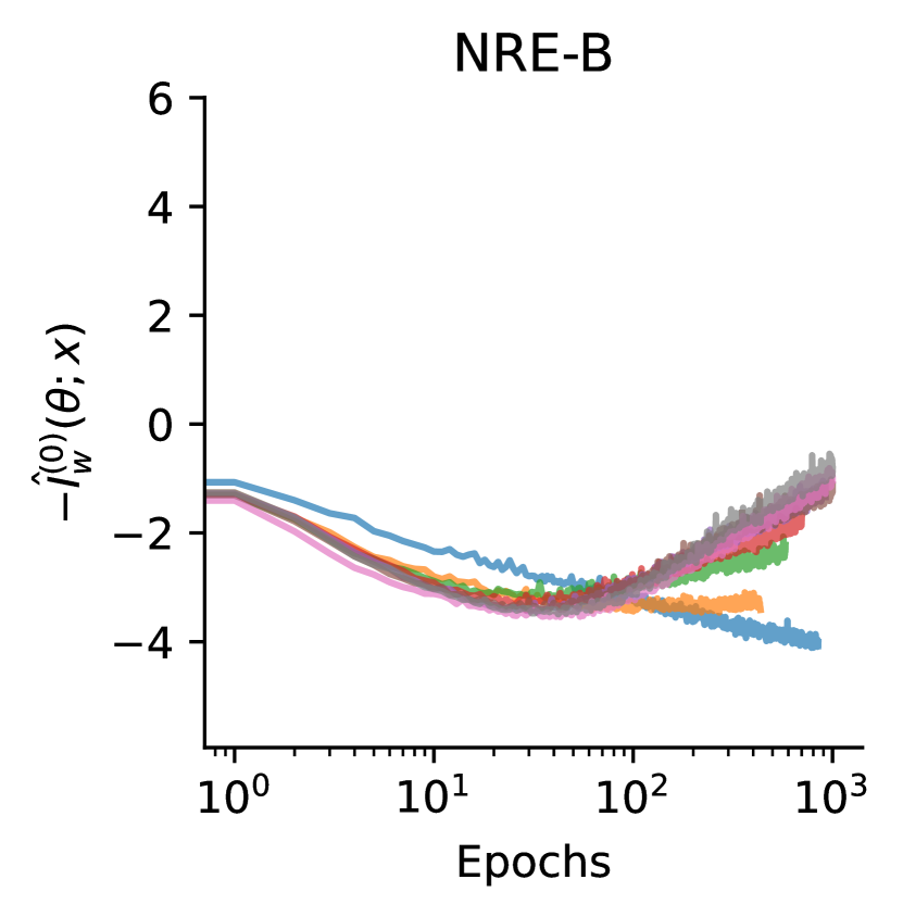
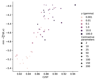
Numerical estimates of the partition function

In addition to bounds on the mutual information, we computed a Monte Carlo estimate of the partition function, $Z_{\boldsymbol{w}}(\boldsymbol{x})$, based on data from the validation set at every epoch during training. The value of the estimated partition function as a function of epoch is shown in Figure 14 for this set of runs on the SLCP task. The estimated $Z_{\boldsymbol{w}}(\boldsymbol{x})$, based on the ratio from nre-b, is completely unconstrained and varies significantly with epoch. nre-c does encourage the partition function to remain “near” unity, although both $\gamma$ and $K$ affect the strength of the encouragement. We find that large numbers of contrastive parameters cause $Z_{\boldsymbol{w}}(\boldsymbol{x})$ to deviate significantly from unity; although, often by tens of orders of magnitude less than nre-b.

This result is connected to the reliability of the importance sampling diagnostic, see Section 2.2. If the partition function is not near unity, then the estimated likelihood-to-evidence ratio does not cancel with the evidence and the diagnostic will behave like nre-b, i.e., it becomes possible to produce accurate, albeit unnormalized, posteriors while failing the diagnostic. This is one reason to limit the number of contrastive parameters.

(a) nre-b

(b) nre-c

Figure 14: Monte Carlo estimate of the partition function $\hat{Z}_{\boldsymbol{w}}(\boldsymbol{x})$ for (a) nre-b and (b) nre-c with various values for $\gamma$ and $K$ on the SLCP inference problem. Note the scale of the ordinate axes. $\hat{Z}_{\boldsymbol{w}}(\boldsymbol{x})$ is completely unconstrained with nre-b; however, it is constrained with nre-c. The strength of encouragement the partition function towards unity depends on the hyperparameters for nre-c. $\hat{Z}_{\boldsymbol{w}}(\boldsymbol{x})$ can still take on extreme values, especially for large number of contrastive examples and large $\gamma$. This represents the same set of experiments as in Figure 4, Figure 4 and Figure 13.

References

- Alsing et al. [2018] J. Alsing, B. Wandelt, and S. Feeney. Massive optimal data compression and density estimation for scalable, likelihood-free inference in cosmology. Monthly Notices of the Royal Astronomical Society, 477(3):2874–2885, 2018.
- Alsing et al. [2019] J. Alsing, T. Charnock, S. Feeney, and B. Wandelt. Fast likelihood-free cosmology with neural density estimators and active learning. Monthly Notices of the Royal Astronomical Society, 488(3):4440–4458, 2019.
- Beaumont et al. [2009] M. A. Beaumont, J.-M. Cornuet, J.-M. Marin, and C. P. Robert. Adaptive approximate bayesian computation. Biometrika, 96(4):983–990, 2009.
- Belghazi et al. [2018] M. I. Belghazi, A. Baratin, S. Rajeswar, S. Ozair, Y. Bengio, A. Courville, and R. D. Hjelm. Mine: mutual information neural estimation. arXiv preprint arXiv:1801.04062, 2018.
- Bishop [2006] C. M. Bishop. Pattern recognition and machine learning (information science and statistics), 2006.
- Blum and François [2010] M. G. Blum and O. François. Non-linear regression models for approximate bayesian computation. Statistics and computing, 20(1):63–73, 2010.
- Brehmer et al. [2018] J. Brehmer, K. Cranmer, G. Louppe, and J. Pavez. Constraining effective field theories with machine learning. Physical review letters, 121(11):111801, 2018.
- Brehmer et al. [2020] J. Brehmer, G. Louppe, J. Pavez, and K. Cranmer. Mining gold from implicit models to improve likelihood-free inference. Proceedings of the National Academy of Sciences, 117(10):5242–5249, 2020.
- Chan et al. [2018] J. Chan, V. Perrone, J. Spence, P. Jenkins, S. Mathieson, and Y. Song. A likelihood-free inference framework for population genetic data using exchangeable neural networks. Advances in neural information processing systems, 31, 2018.
- Cole et al. [2021] A. Cole, B. K. Miller, S. J. Witte, M. X. Cai, M. W. Grootes, F. Nattino, and C. Weniger. Fast and credible likelihood-free cosmology with truncated marginal neural ratio estimation. arXiv preprint arXiv:2111.08030, 2021.
- Coogan et al. [2020] A. Coogan, K. Karchev, and C. Weniger. Targeted likelihood-free inference of dark matter substructure in strongly-lensed galaxies. arXiv preprint arXiv:2010.07032, 2020.
- Cranmer et al. [2015] K. Cranmer, J. Pavez, and G. Louppe. Approximating likelihood ratios with calibrated discriminative classifiers. arXiv preprint arXiv:1506.02169, 2015.
- Cranmer et al. [2020] K. Cranmer, J. Brehmer, and G. Louppe. The frontier of simulation-based inference. Proc. Natl. Acad. Sci. U. S. A., May 2020.
- Dalmasso et al. [2020] N. Dalmasso, R. Izbicki, and A. Lee. Confidence sets and hypothesis testing in a likelihood-free inference setting. In International Conference on Machine Learning, pages 2323–2334. PMLR, 2020.
- Drovandi et al. [2018] C. C. Drovandi, C. Grazian, K. Mengersen, and C. Robert. Approximating the likelihood in abc. Handbook of approximate bayesian computation, pages 321–368, 2018.
- Durkan et al. [2020] C. Durkan, I. Murray, and G. Papamakarios. On contrastive learning for likelihood-free inference. In International Conference on Machine Learning, pages 2771–2781. PMLR, 2020.
- Friedman [2003] J. H. Friedman. On multivariate goodness–of–fit and two–sample testing. STATISTICAL PROBLEMS IN PARTICLE PHYSICS, ASTROPHYSICS AND COSMOLOGY, page 311, 2003.
- Glöckler et al. [2021] M. Glöckler, M. Deistler, and J. H. Macke. Variational methods for simulation-based inference. In International Conference on Learning Representations, 2021.
- Goodfellow et al. [2020] I. Goodfellow, J. Pouget-Abadie, M. Mirza, B. Xu, D. Warde-Farley, S. Ozair, A. Courville, and Y. Bengio. Generative adversarial networks. Communications of the ACM, 63(11):139–144, 2020.
- Gratton [2017] S. Gratton. Glass: A general likelihood approximate solution scheme. arXiv preprint arXiv:1708.08479, 2017.
- Greenberg et al. [2019] D. Greenberg, M. Nonnenmacher, and J. Macke. Automatic posterior transformation for likelihood-free inference. In International Conference on Machine Learning, pages 2404–2414. PMLR, 2019.
- Gutmann and Hyvärinen [2010] M. Gutmann and A. Hyvärinen. Noise-contrastive estimation: A new estimation principle for unnormalized statistical models. In Proceedings of the thirteenth international conference on artificial intelligence and statistics, pages 297–304. JMLR Workshop and Conference Proceedings, 2010.
- Gutmann and Hyvärinen [2012] M. U. Gutmann and A. Hyvärinen. Noise-contrastive estimation of unnormalized statistical models, with applications to natural image statistics. Journal of machine learning research, 13(2), 2012.
- Gutmann et al. [2016] M. U. Gutmann, J. Corander, et al. Bayesian optimization for likelihood-free inference of simulator-based statistical models. Journal of Machine Learning Research, 2016.
- Gutmann et al. [2022] M. U. Gutmann, S. Kleinegesse, and B. Rhodes. Statistical applications of contrastive learning. arXiv preprint arXiv:2204.13999, 2022.
- Harris et al. [2020] C. R. Harris, K. J. Millman, S. J. van der Walt, R. Gommers, P. Virtanen, D. Cournapeau, E. Wieser, J. Taylor, S. Berg, N. J. Smith, R. Kern, M. Picus, S. Hoyer, M. H. van Kerkwijk, M. Brett, A. Haldane, J. F. del R’ıo, M. Wiebe, P. Peterson, P. G’erard-Marchant, K. Sheppard, T. Reddy, W. Weckesser, H. Abbasi, C. Gohlke, and T. E. Oliphant. Array programming with NumPy. Nature, 585(7825):357–362, Sept. 2020. doi: 10.1038/s41586-020-2649-2. URL https://doi.org/10.1038/s41586-020-2649-2.
- Hastie et al. [2009] T. Hastie, R. Tibshirani, J. H. Friedman, and J. H. Friedman. The elements of statistical learning: data mining, inference, and prediction, volume 2. Springer, 2009.
- He et al. [2016] K. He, X. Zhang, S. Ren, and J. Sun. Deep residual learning for image recognition. In 2016 IEEE Conference on Computer Vision and Pattern Recognition (CVPR), pages 770–778, 2016. doi: 10.1109/CVPR.2016.90.
- Hermans et al. [2020a] J. Hermans, N. Banik, C. Weniger, G. Bertone, and G. Louppe. Towards constraining warm dark matter with stellar streams through neural simulation-based inference. arXiv preprint arXiv:2011.14923, 2020a.
- Hermans et al. [2020b] J. Hermans, V. Begy, and G. Louppe. Likelihood-free mcmc with amortized approximate ratio estimators. In International Conference on Machine Learning, pages 4239–4248. PMLR, 2020b.
- Hermans et al. [2021] J. Hermans, A. Delaunoy, F. Rozet, A. Wehenkel, and G. Louppe. Averting a crisis in simulation-based inference. arXiv preprint arXiv:2110.06581, 2021.
- Hunter [2007] J. D. Hunter. Matplotlib: A 2d graphics environment. Computing in Science & Engineering, 9(3):90–95, 2007. doi: 10.1109/MCSE.2007.55.
- Ioffe and Szegedy [2015] S. Ioffe and C. Szegedy. Batch normalization: Accelerating deep network training by reducing internal covariate shift. In International conference on machine learning, pages 448–456. PMLR, 2015.
- Izbicki et al. [2014] R. Izbicki, A. Lee, and C. Schafer. High-dimensional density ratio estimation with extensions to approximate likelihood computation. In Artificial intelligence and statistics, pages 420–429. PMLR, 2014.
- Järvenpää et al. [2021] M. Järvenpää, M. U. Gutmann, A. Vehtari, and P. Marttinen. Parallel gaussian process surrogate bayesian inference with noisy likelihood evaluations. Bayesian Analysis, 16(1):147–178, 2021.
- Jeffrey and Wandelt [2020] N. Jeffrey and B. D. Wandelt. Solving high-dimensional parameter inference: marginal posterior densities & moment networks. arXiv preprint arXiv:2011.05991, 2020.
- Kingma and Ba [2015] D. P. Kingma and J. L. Ba. Adam: A method for stochastic gradient descent. In ICLR: International Conference on Learning Representations, pages 1–15, 2015.
- Kluyver et al. [2016] T. Kluyver, B. Ragan-Kelley, F. Pérez, B. Granger, M. Bussonnier, J. Frederic, K. Kelley, J. Hamrick, J. Grout, S. Corlay, P. Ivanov, D. Avila, S. Abdalla, C. Willing, and J. development team. Jupyter notebooks - a publishing format for reproducible computational workflows. In F. Loizides and B. Scmidt, editors, Positioning and Power in Academic Publishing: Players, Agents and Agendas, pages 87–90, Netherlands, 2016. IOS Press. URL https://eprints.soton.ac.uk/403913/.
- Lacoste et al. [2019] A. Lacoste, A. Luccioni, V. Schmidt, and T. Dandres. Quantifying the carbon emissions of machine learning. arXiv preprint arXiv:1910.09700, 2019.
- Lehmann et al. [2005] E. L. Lehmann, J. P. Romano, and G. Casella. Testing statistical hypotheses, volume 3. Springer, 2005.
- Lopez-Paz and Oquab [2017] D. Lopez-Paz and M. Oquab. Revisiting classifier two-sample tests. In International Conference on Learning Representations, 2017.
- Lueckmann et al. [2017] J.-M. Lueckmann, P. J. Gonçalves, G. Bassetto, K. Öcal, M. Nonnenmacher, and J. H. Macke. Flexible statistical inference for mechanistic models of neural dynamics. In Proceedings of the 31st International Conference on Neural Information Processing Systems, pages 1289–1299, 2017.
- Lueckmann et al. [2019] J.-M. Lueckmann, G. Bassetto, T. Karaletsos, and J. H. Macke. Likelihood-free inference with emulator networks. In Symposium on Advances in Approximate Bayesian Inference, pages 32–53. PMLR, 2019.
- Lueckmann et al. [2021] J.-M. Lueckmann, J. Boelts, D. Greenberg, P. Goncalves, and J. Macke. Benchmarking simulation-based inference. In A. Banerjee and K. Fukumizu, editors, Proceedings of The 24th International Conference on Artificial Intelligence and Statistics, volume 130 of Proceedings of Machine Learning Research, pages 343–351. PMLR, 13–15 Apr 2021. URL http://proceedings.mlr.press/v130/lueckmann21a.html.
- Ma and Collins [2018] Z. Ma and M. Collins. Noise contrastive estimation and negative sampling for conditional models: Consistency and statistical efficiency. In Proceedings of the 2018 Conference on Empirical Methods in Natural Language Processing, pages 3698–3707, 2018.
- Mikolov et al. [2013] T. Mikolov, I. Sutskever, K. Chen, G. S. Corrado, and J. Dean. Distributed representations of words and phrases and their compositionality. Advances in neural information processing systems, 26, 2013.
- Miller et al. [2020] B. K. Miller, A. Cole, G. Louppe, and C. Weniger. Simulation-efficient marginal posterior estimation with swyft: stop wasting your precious time. arXiv preprint arXiv:2011.13951, 2020.
- Miller et al. [2021] B. K. Miller, A. Cole, P. Forré, G. Louppe, and C. Weniger. Truncated marginal neural ratio estimation. Advances in Neural Information Processing Systems, 34:129–143, 2021.
- Mnih and Teh [2012] A. Mnih and Y. W. Teh. A fast and simple algorithm for training neural probabilistic language models. In Proceedings of the 29th International Coference on International Conference on Machine Learning, pages 419–426, 2012.
- Mohamed and Lakshminarayanan [2016] S. Mohamed and B. Lakshminarayanan. Learning in implicit generative models. arXiv preprint arXiv:1610.03483, 2016.
- Neal [2003] R. M. Neal. Slice sampling. Annals of statistics, pages 705–741, 2003.
- pandas development team [2020] T. pandas development team. pandas-dev/pandas: Pandas, Feb. 2020. URL https://doi.org/10.5281/zenodo.3509134.
- Papamakarios and Murray [2016] G. Papamakarios and I. Murray. Fast -free inference of simulation models with bayesian conditional density estimation. Advances in neural information processing systems, 29, 2016.
- Papamakarios et al. [2017] G. Papamakarios, T. Pavlakou, and I. Murray. Masked autoregressive flow for density estimation. In Proceedings of the 31st International Conference on Neural Information Processing Systems, pages 2335–2344, 2017.
- Papamakarios et al. [2019a] G. Papamakarios, E. Nalisnick, D. J. Rezende, S. Mohamed, and B. Lakshminarayanan. Normalizing flows for probabilistic modeling and inference. arXiv preprint arXiv:1912.02762, 2019a.
- Papamakarios et al. [2019b] G. Papamakarios, D. Sterratt, and I. Murray. Sequential neural likelihood: Fast likelihood-free inference with autoregressive flows. In The 22nd International Conference on Artificial Intelligence and Statistics, pages 837–848. PMLR, 2019b.
- Paszke et al. [2019] A. Paszke, S. Gross, F. Massa, A. Lerer, J. Bradbury, G. Chanan, T. Killeen, Z. Lin, N. Gimelshein, L. Antiga, A. Desmaison, A. Kopf, E. Yang, Z. DeVito, M. Raison, A. Tejani, S. Chilamkurthy, B. Steiner, L. Fang, J. Bai, and S. Chintala. Pytorch: An imperative style, high-performance deep learning library. In H. Wallach, H. Larochelle, A. Beygelzimer, F. d Alché-Buc, E. Fox, and R. Garnett, editors, Advances in Neural Information Processing Systems 32, pages 8024–8035. Curran Associates, Inc., 2019. URL http://papers.neurips.cc/paper/9015-pytorch-an-imperative-style-high-performance-deep-learning-library.pdf.
- Poole et al. [2019] B. Poole, S. Ozair, A. Van Den Oord, A. Alemi, and G. Tucker. On variational bounds of mutual information. In International Conference on Machine Learning, pages 5171–5180. PMLR, 2019.
- Prangle [2019] D. Prangle. Distilling importance sampling. arXiv preprint arXiv:1910.03632, 2019.
- Ramesh et al. [2021] P. Ramesh, J.-M. Lueckmann, J. Boelts, Á. Tejero-Cantero, D. S. Greenberg, P. J. Goncalves, and J. H. Macke. Gatsbi: Generative adversarial training for simulation-based inference. In International Conference on Learning Representations, 2021.
- Rodrigues et al. [2020] G. Rodrigues, D. J. Nott, and S. A. Sisson. Likelihood-free approximate gibbs sampling. Statistics and Computing, 30(4):1057–1073, 2020.
- Shimodaira [2000] H. Shimodaira. Improving predictive inference under covariate shift by weighting the log-likelihood function. Journal of statistical planning and inference, 90(2):227–244, 2000.
- Simola et al. [2020] U. Simola, J. Corander, and U. Picchini. Adaptive mcmc for synthetic likelihoods and correlated synthetic likelihoods. Bayesian analysis, 2020.
- Sisson et al. [2018] S. A. Sisson, Y. Fan, and M. Beaumont. Handbook of approximate Bayesian computation. CRC Press, 2018.
- Skilling [2006] J. Skilling. Nested sampling for general bayesian computation. Bayesian Anal., 1(4):833–859, Dec. 2006.
- Sugiyama et al. [2012] M. Sugiyama, T. Suzuki, and T. Kanamori. Density ratio estimation in machine learning. Cambridge University Press, 2012.
- Talts et al. [2018] S. Talts, M. Betancourt, D. Simpson, A. Vehtari, and A. Gelman. Validating bayesian inference algorithms with simulation-based calibration. arXiv preprint arXiv:1804.06788, 2018.
- Tejero-Cantero et al. [2020] A. Tejero-Cantero, J. Boelts, M. Deistler, J.-M. Lueckmann, C. Durkan, P. J. Gonçalves, D. S. Greenberg, and J. H. Macke. sbi: A toolkit for simulation-based inference. Journal of Open Source Software, 5(52):2505, 2020. doi: 10.21105/joss.02505. URL https://doi.org/10.21105/joss.02505.
- Thomas et al. [2016] O. Thomas, R. Dutta, J. Corander, S. Kaski, M. U. Gutmann, et al. Likelihood-free inference by ratio estimation. Bayesian Analysis, 2016.
- Toni et al. [2009] T. Toni, D. Welch, N. Strelkowa, A. Ipsen, and M. P. H. Stumpf. Approximate bayesian computation scheme for parameter inference and model selection in dynamical systems. J. R. Soc. Interface, 6(31):187–202, Feb. 2009.
- Van den Oord et al. [2018] A. Van den Oord, Y. Li, and O. Vinyals. Representation learning with contrastive predictive coding. arXiv e-prints, pages arXiv–1807, 2018.
- Virtanen et al. [2020] P. Virtanen, R. Gommers, T. E. Oliphant, M. Haberland, T. Reddy, D. Cournapeau, E. Burovski, P. Peterson, W. Weckesser, J. Bright, S. J. van der Walt, M. Brett, J. Wilson, K. J. Millman, N. Mayorov, A. R. J. Nelson, E. Jones, R. Kern, E. Larson, C. J. Carey, İ. Polat, Y. Feng, E. W. Moore, J. VanderPlas, D. Laxalde, J. Perktold, R. Cimrman, I. Henriksen, E. A. Quintero, C. R. Harris, A. M. Archibald, A. H. Ribeiro, F. Pedregosa, P. van Mulbregt, and SciPy 1.0 Contributors. SciPy 1.0: Fundamental Algorithms for Scientific Computing in Python. Nature Methods, 17:261–272, 2020. doi: 10.1038/s41592-019-0686-2.
- Waskom [2021] M. L. Waskom. seaborn: statistical data visualization. Journal of Open Source Software, 6(60):3021, 2021. doi: 10.21105/joss.03021. URL https://doi.org/10.21105/joss.03021.
- Wes McKinney [2010] Wes McKinney. Data Structures for Statistical Computing in Python. In Stéfan van der Walt and Jarrod Millman, editors, Proceedings of the 9th Python in Science Conference, pages 56 – 61, 2010. doi: 10.25080/Majora-92bf1922-00a.