Efficient Gaussian Process Model on Class-Imbalanced Datasets
for Generalized Zero-Shot Learning

Abstract

Zero-Shot Learning (ZSL) models aim to classify object classes that are not seen during the training process. However, the problem of class imbalance is rarely discussed, despite its presence in several ZSL datasets. In this paper, we propose a Neural Network model that learns a latent feature embedding and a Gaussian Process (GP) regression model that predicts latent feature prototypes of unseen classes. A calibrated classifier is then constructed for ZSL and Generalized ZSL tasks. Our Neural Network model is trained efficiently with a simple training strategy that mitigates the impact of class-imbalanced training data. The model has an average training time of 5 minutes and can achieve state-of-the-art (SOTA) performance on imbalanced ZSL benchmark datasets like AWA2, AWA1 and APY, while having relatively good performance on the SUN and CUB datasets.

I Introduction

Zero-Shot Learning (ZSL) requires a model to be trained on images that show examples from one set of classes, referred to as seen classes, while being tested on images that show examples from another set of classes, referred to as unseen classes. During training, semantic information for both seen classes and unseen classes is provided to help infer the appearance of unseen classes.

Many previous works, such as [1, 2, 3, 4, 5], focus on learning a mapping between image features depicting certain classes and their corresponding semantic vectors. GFZSL [3] proposed a model similar to Kernel Ridge Regression to predict image features of unseen classes. GDAN [4] and f-CLSWGAN [5] utilize generative models like GAN [6] and VAE [7] to achieve the same objective.

On the basis of these approaches, recent papers further learn a Neural Network (NN) projection from image feature space to a latent embedding space, where inter-class features can be better separated within each ZSL dataset [8, 9, 10, 11, 12]. For example, in [9], image features are projected to a latent space in order to “remove redundant information”. FREE [10] adopts the same structure for “feature refinement” purposes. CE-GZSL [12] also proposes a similar approach to generate a “contrastive embedding” of image features.

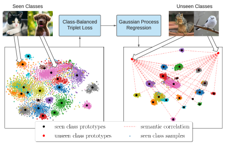
Figure 1: We first train a latent embedding model for image features. The model is trained with Class-Balanced Triplet loss in order to separate inter-class features, which is robust to class-imbalanced datasets. Then a Gaussian Process Regression model is proposed to predict unseen class prototypes based on seen class prototypes and semantic correlations between classes. Finally, our ZSL classifier is constructed based on the prototypes.

Previous models, however, do not typically concern themselves with the class-imbalanced data distributions of ZSL datasets. In the real visual world, visual datasets usually exhibit an imbalanced data distribution among categories [13]. In supervised learning, the class imbalance problem can have significant impact on the performance of classification models [14, 15]. For the ZSL problem, the APY [16] dataset has nearly $1/3$ of samples belonging to the same class. AWA2 [17] has 1645 samples in one class and only 100 samples in another. Clearly, the class imbalance problem is not negligible when training a classification model on these datasets.

On the other hand, recent models usually have complicated structures that require strong regularizers in order to prevent overfitting on seen class samples. As a consequence, these models usually have long training times and heavy GPU memory usage. The average training time for DVBE [11] is over 2 hours on each ZSL dataset. This fact motivates us to search for alternative models that are simpler and less prone to overfitting.

In this paper, we adopt the idea of projecting image features in a latent embedding space via a Neural Network (NN) model. We propose a class-balanced triplet loss that separate image features in a latent embedding space for class-imbalanced datasets. We also propose a Gaussian Process (GP) model to learn a mapping between features and a semantic space. The classical Gaussian Process (GP), when used in the setting of regression, is robust to overfitting [18]. If training and testing data come from the same distribution, a PAC-Bayesian Bound [19] guarantees that the training error will be close to the testing error.

Our experiments demonstrate that our model, though employing a simple design, can reach SOTA performance on the class-imbalanced ZSL datasets AWA1, AWA2 and APY in the Generalized ZSL setting.

The main contributions of our work are:

1. We propose a novel simple framework for ZSL, where image features from a deep Neural Network are mapped into a latent embedding space to generate latent prototypes for each seen class by a novel triplet training model. Then a Gaussian Process (GP) regression model is trained via maximizing the marginal likelihood to predict latent prototypes of unseen classes.

2. The mapping from image features to a latent space is performed by our proposed triplet training model for ZSL learning, using a novel triplet loss that is robust on class-imbalanced ZSL datasets. Our experiments show improved performance over the traditional triplet loss on all ZSL datasets, including SOTA performance on class-imbalanced datasets, specifically, AWA1, AWA2 and APY.

3. Given feature vectors extracted by a pre-trained ResNet, our model has an average training time of 5 minutes on all ZSL datasets, faster than several SOTA models that have high accuracy.

II Related Works

Traditional and Generalized ZSL: Early ZSL research adopts a so-called Traditional ZSL setting [1, 20]. The Traditional ZSL requires the model to train on images of seen classes and semantic vectors of seen and unseen classes. Test images are restricted to the unseen classes. However, in practice, test images may also come from the seen classes [17]. The Generalized ZSL setting was proposed to address the problem of including both seen and unseen images in the test set. According to Xian et al.  [17], models that have good performance in the Traditional ZSL setting may not work well in the Generalized ZSL setting.

Prototypical Methods. Our classification model is related to prototypical methods proposed in Zero-Shot and Few-Shot learning [21, 22, 23]. In the prototypical methods, a prototype is learned for each class to help classification. For example, Snell et al. [21] propose a neural network to learn a projection from semantic vectors to feature prototypes of each class. Test samples are classified via Nearest Neighbor among prototypes. While the classification process of our model is similar to prototypical methods, our model uses a Gaussian Process Regression instead of Neural Networks to predict prototypes of unseen classes.

Inductive and Transductive ZSL: Similar to most ZSL models, the model we propose is an inductive ZSL model. Inductive ZSL requires that no feature information of unseen classes is present during the training phase [17]. Models that introduce unlabeled unseen images during the training phase are called transductive ZSL models [24]. Ensuring a fair comparison, results from such models are usually compared separately to inductive models since additional information is introduced [3, 25, 26].

Triplet Loss. Many ZSL models have proposed a triplet loss in their framework to help separate samples from different classes. Chacheux et al. [8] proposed a variant of a triplet loss in their model to learn feature prototypes for different classes. Han et al. [9] adopt an improved version of the triplet loss called “center loss” proposed in [27] that separates samples in a latent space. Unlike their models, we notice that current triplet losses proposed for the ZSL problem may not perform well on class-imbalanced datasets like AWA2, AWA1 and APY. An improved version of the triplet loss training model is proposed to mitigate this problem.

Gaussian Process Regression. For the ZSL problem, Dolma et al. [28] proposed a model that performs k-nearest neighbor search for test samples over training samples and performs a GP regression based on the search result. Mukherjee et al. [29] model image features and semantic vectors for each class with Gaussians, and learns a linear projection between the two distributions. Our model is closest to Elhoseiny et al. [30], where Gaussian Process Regression is used to predict unseen class prototypes based on seen class prototypes. However, they used a Gaussian Process directly without the benefit of a learned network model for feature embedding, and showed relatively poor results. Verma and Rai [3] proposed a Kernel Ridge Regression (KRR) approach called GFZSL for the traditional ZSL problem. Our experiment demonstrates that our model outperforms GFZSL by a large margin.

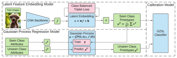
Figure 2: Structure of our proposed model. Feature vectors $\mathbf{f}$ are projected to a latent embedding space $\mathbf{x}$ which is trained using proposed Class-Balanced Triplet Loss. A GP model is proposed to predict latent prototypes of unseen classes $\mathbf{\mu}^{U}$, based on latent prototypes of seen class $\mathbf{\mu}^{S}$ and semantic vectors from seen and unseen class $\mathbf{s}^{S},\mathbf{s}^{U}$.

III Proposed Approach

We propose a hybrid model for the ZSL problem: a Latent Feature Embedding model to separate inter-class features that is robust to class-imbalanced datasets, a GP Regression model to predict prototypes of unseen classes based on seen classes and semantic information and a calibrated classifier to balance the trade-off between seen and unseen class accuracy.

III-A Latent Feature Embedding Model

Model Structure We propose to learn a linear NN mapping from image features to latent embeddings. We argue that for the ZSL task, a linear projection with limited flexibility can help prevent the model from overfitting on seen class training samples. Following others [3, 28], we model feature vectors from each class using the multivariate Gaussian distribution. We exploit the fact that Gaussian random vectors are closed under linear transformations.

For each feature vector $\mathbf{f}\in\mathbb{R}^{N_{feature}}$, the latent embedding $\mathbf{x}\in\mathbb{R}^{N_{latent}}$ can be written as:

$$\mathbf{x}=\mathbf{wf}+\mathbf{b}.$$ (1)

Here $\mathbf{w}\in\mathbb{R}^{N_{latent}\times N_{feature}}$ is a weight parameter matrix and $\mathbf{b}\in\mathbb{R}^{N_{latent}}$ is a bias parameter vector.

Triplet Loss Revisited Triplet loss is often used to separate samples from different training classes in the dataset [31]. The standard triplet loss aims to decrease distances between intra-class samples and increase distances between inter-class samples.

In each iteration, a mini-batch is sampled uniformly from training data as: $\{\mathbf{x}^{c_{1}}_{1},\mathbf{x}^{c_{1}}_{2},...,\mathbf{x}^{c_{1}}_{n^{c_{1}}},\mathbf{x}^{c_{2}}_{1},\mathbf{x}^{c_{2}}_{2},...\mathbf{x}^{c_{2}}_{n^{c_{2}}},...\mathbf{x}^{c_{L}}_{n^{c_{L}}}\}$. Here $\mathbf{x}^{c_{i}}_{j}$ denotes the $j^{th}$ our of total $n^{c_{i}}\in\mathbb{Z}^{+}$ samples that belongs to training class $c_{i}\in C,i=1,2,...,L$ in mini-batch. The batch size is $N=\sum n^{c_{j}}$. Then all possible triplet pairs $\{\mathbf{x}^{c_{i}}_{l},\mathbf{x}^{c_{i}}_{m},\mathbf{x}^{c_{j}}_{n}\}$ are constructed within the given mini-batch. In each triplet, $\mathbf{x}^{c_{i}}_{l},\mathbf{x}^{c_{i}}_{m}$ are different samples from the same class $c_{i}$, $l,m\in[1,2,...,n^{c_{i}}]$, $\mathbf{x}^{c_{j}}_{n}$ come from a different class $c_{i}\neq c_{j}$, $n\in[1,2,...,n^{c_{j}}]$. The triplet loss is written as:

$$\mathcal{L}_{T}=\sum_{c_{i},c_{j}}\sum^{n^{c_{i}}}_{l=1}\sum^{n^{c_{i}}-1}_{m=1}\sum_{n=1}^{n^{c_{j}}}\max(0,\Delta+(\mathbf{x}_{l}^{c_{i}}-\mathbf{x}_{m}^{c_{i}})^{2}-(\mathbf{x}_{l}^{c_{i}}-\mathbf{x}_{n}^{c_{j}})^{2}).$$ (2)

The $\sum_{c_{i},c_{j}}$ denotes summation over all training class pairs $c_{i},c_{j}\in C$ that have $c_{i}\neq c_{j}$. Hyperparameter $\Delta\in\mathbb{R}^{+}$ is a positive threshold that balances the inter and intra class distances [8, 32].

The class imbalance problem is not considered in the original triplet loss. Moreover, models trained with a triplet loss usually require many iterations until convergence, expensive memory requirements and a high variance [32]. We thus propose a new Class-Balanced Triplet loss to mitigate these problems.

Class-Balanced Triplet Loss When training a model with a triplet loss, a straight forward approach to tackle the class imbalance problem is to sample class-balanced mini-batch data. The model will not be affected by the class imbalance problem if it is trained using class-balanced data.

In every iteration, unlike for the traditional triplet loss, we generate a class-balanced mini-batch by sampling $n^{CB}\in\mathbb{Z}^{+}$ data points from each one of $L$ training classes in the training set as $\{\mathbf{x}^{c_{1}}_{1},\mathbf{x}^{c_{1}}_{2},...,\mathbf{x}^{c_{1}}_{n^{CB}},\mathbf{x}^{c_{2}}_{1},\mathbf{x}^{c_{2}}_{2},...\mathbf{x}^{c_{2}}_{n^{CB}},...\mathbf{x}^{c_{L}}_{n^{CB}}\}$. The batch size becomes $N=n^{CB}\times L$. In a supervised classification setting, similar approaches have shown to be effective [14].

We then propose a modified triplet loss $L_{BT}$ to train the model on the mini-batch. For every mini-batch, the loss has the form:

$$\mathcal{L}_{BT}=\sum_{c_{i},c_{j}}\sum_{l=1}^{n^{CB}}\max(0,\Delta+(\mathbf{x}_{l}^{c_{i}}-\overline{\mathbf{x}^{c_{i}}})^{2}-\min_{n}(\mathbf{x}_{n}^{c_{j}}-\overline{\mathbf{x}^{c_{i}}})^{2}).$$ (3)

The term $\overline{\mathbf{x}^{c_{i}}}=\frac{1}{n^{c}}\sum_{n}\mathbf{x}^{c_{i}}_{n}$ denotes the average of samples from class $c_{i}$ in the mini-batch. Replacing the term $\mathbf{x}_{m}^{c_{i}}$ with $\overline{\mathbf{x}^{c_{i}}}$ in the original triplet loss can help reduce the variance in the loss during training, which is similar to “center loss” [27]. However, unlike their method, we are not adding extra trainable parameters into the model. The $\min()$ operation is performed over all samples $\mathbf{x}^{c_{j}}_{m}$ in class $c_{j}$ in the mini-batch, which can efficiently reduce computational costs.

With the help of the proposed triplet loss $\mathcal{L}_{BT}$, our model can efficiently learn a latent embedding that separates samples from different classes and maintains a good performance on imbalanced datasets.

III-B Gaussian Process (GP) Regression Model

We propose a GP Regression model to predict prototypes of unseen classes, leveraging the generalization ability of GP models. Like Mukherjee et al. [29], we obtain the average of all latent features in each class $\mathbf{\mu}^{c_{i}}=\frac{1}{N^{c_{i}}}\sum\mathbf{x}^{c_{i}}$ as a prototype for the corresponding class.

We also denote semantic vector of each class $s^{c_{i}}\in\mathbb{R}^{N_{semantic}}$. Given the semantic vectors $\mathbf{s}^{S}=[\mathbf{s}^{c_{1}},...\mathbf{s}^{c_{L}}]^{T}$ and feature prototypes $\mathbf{\mu}^{S}=[\mathbf{\mu}^{c_{1}},...\mathbf{\mu}^{c_{L}}]^{T}$ for seen class $c_{1},c_{2},...c_{L}\in C^{S}$, along with semantic vectors $\mathbf{s}^{U}=[\mathbf{s}^{c_{L+1}},...\mathbf{s}^{c_{L+K}}]^{T}$ for unseen classes $c_{L+1},c_{L+2},...c_{L+K}\in C^{U}$, we can use the GPR model to regress prototypes $\mu^{U}=[\mathbf{\mu}^{c_{L+1}},...\mathbf{\mu}^{c_{L+K}}]^{T}$ for unseen classes $c\in C^{U}$:

$$\mathbf{\mu}^{U}=f_{GP}(\mathbf{s}^{U}|\theta)+\epsilon.$$ (4)

Here $f_{GP}(\mathbf{s}|\theta)$ is the regression function, $\epsilon\sim\mathcal{N}(0,\sigma^{2})$ denotes the Gaussian random noise and $\theta$ is the hyperparameter in the model. $\theta$ is trained given seen class semantic vectors $\mathbf{s}^{S}$ and corresponding prototypes $\mu^{S}$.

Directly training a GPR model that learns a projection from $\mathbf{s}$ to $\mathbf{\mu}$ requires accounting for every dimension in $\mathbf{\mu}\in\mathbb{R}^{N_{latent}}$, which is computationally expensive because the model needs to estimate correlations between different dimensions. We propose to avoid this issue by assuming dimensions in $\mathbf{\mu}^{c}$ are independent from each other so that the GPR model can be applied to $\mathbf{\mu}_{i}$:

$$\mathbf{\mu}^{U}_{i}=f_{GP}(\mathbf{s}^{U}|\theta_{i})+\epsilon_{i}.$$ (5)

Then we have hyperparameter $\theta_{i}$ and noise $\epsilon_{i}$ for $i^{th}$ dimension in $\mu$.

A Gaussian Process is defined by a mean function $m(\mathbf{s})$ and a covariance function $k(\mathbf{s},\mathbf{s}^{\prime}|\theta)$ that depends on hyperparameter $\theta$. For $f_{GP}(\mathbf{s}|\theta_{i})$, a GP can be written as:

$$f_{GP}(\mathbf{s}|\theta_{i})\sim\mathcal{GP}(\mathbf{m}(\mathbf{s}),k(\mathbf{s},\mathbf{s}^{\prime}|\theta_{i})).$$ (6)

Here we will take $\mathbf{m}\equiv 0$. The joint prior distribution of seen class prototypes $\mathbf{\mu}_{i}^{S}$ and regression function $f_{GP}(\mathbf{s}|\theta_{i})$ can be written as:

$$\begin{bmatrix}f_{GP}\\ {\mathbf{\mu}}_{i}^{S}\end{bmatrix}\sim\mathcal{N}\left(\mathbf{0},\begin{bmatrix}k(\mathbf{s},\mathbf{s}|\theta_{i})&k(\mathbf{s},\mathbf{s}^{S}|\theta_{i})\\ k(\mathbf{s}^{S},\mathbf{s}|\theta_{i})&k(\mathbf{s}^{S},\mathbf{s}^{S}|\theta_{i})+\mathbf{I}\sigma_{i}^{2}\end{bmatrix}\right),$$ (7)

where $\mathbf{I}$ denotes the identity matrix. $f_{GP}=f_{GP}(\mathbf{s}|\theta_{i})$ can be obtained via conditioning the joint prior distribution on $\mathbf{\mu}^{S}_{i}$ to obtain the posterior predictive distribution, which is also a Gaussian distribution $f_{GP}(\mathbf{s}|\theta_{i})|\mathbf{\mu}_{i}^{S},\mathbf{s}^{S}\sim\mathcal{N}(\mathbf{m}_{i},\Sigma)$. We use the mean $\mathbf{m}_{i}$ of the predictive posterior distribution to form our prediction of $f_{GP}(\mathbf{s}|\theta_{i})$ evaluated at the unseen classes $\mathbf{s}=\mathbf{s}^{U}$, which gives:

$$f_{GP}(\mathbf{s}|\theta_{i})=\mathbf{m}_{i}(\mathbf{s})=k(\mathbf{s},\mathbf{s}^{S}|\theta_{i})\left[k(\mathbf{s}^{S},\mathbf{s}^{S}|\theta_{i})+\mathbf{I}\sigma_{i}^{2}\right]^{-1}\mu_{i}^{S}.$$ (8)

Any positive semi-definite kernel function may be used as a covariance function $k(\mathbf{s},\mathbf{s}^{\prime}|\theta_{i})$, with $\theta_{i}$ as a hyperparameter in the kernel. We propose to search for optimal hyperparameters $\theta_{i}$ for each feature dimension $i$ by maximizing the log marginal likelihoods:

$$\theta_{i}=\arg\max_{\theta_{i}} \Bigg{(}-\frac{1}{2}(\mathbf{\mu}_{i}^{S})^{T}\left[k(\mathbf{s}^{S},\mathbf{s}^{S}|\theta_{i})+\mathbf{I}\sigma_{i}^{2}\right]^{-1}\mathbf{\mu}_{i}^{S}\Bigg{.}$$ (9)

$$\Bigg{.}-\frac{1}{2}\log k(\mathbf{s}^{S},\mathbf{s}^{S}|\theta_{i})\Bigg{)}.$$

With $\theta_{i}$ given, unseen class prototypes can be evaluate by $\mu_{i}^{U}=f_{GP}(\mathbf{s}|\theta_{i})$. Similar to other prototypical methods, the classifier can then be constructed using a nearest neighbor approach based on a distance metric. We use the Euclidean distance in our model:

$$predict(\mathbf{x})=\arg\min_{c\in C}||\mathbf{x}-\mu^{c}||^{2}.$$ (10)

III-C Calibration

It is well known that ZSL models trained on seen classes are inclined to be biased towards classifying unseen images into seen classes [33, 34]. Therefore, it is necessary to add a penalty term $\gamma\in\mathbb{R}^{+}$ when computing classification metrics over seen classes $c_{i}\in C^{S}$. We adopt the calibration approach proposed by Cacheux et al. [33]. The calibrated nearest neighbor classifier is then written as:

$$predict(\mathbf{x})=\arg\max_{c\in C}[-||\mathbf{x}-\mathbf{\mu}^{c}||^{2}-\gamma\mathds{1}_{c\in C^{S}}].$$ (11)

where $\mathds{1}_{c_{i}\in C_{S}}$ is the indicator function, which equals to 1 when class $c$ is from a seen class and 0 otherwise.

In our model, we first use the GPR model to predict the validation class based on the training class, then we train $\gamma$ as a calibration penalty to maximize the harmonic mean. After training, the test class is predicted and conditioned on training classes and validation classes together, and $\gamma$ is used for calibration evaluation of the performance on the test set.

IV Experiments

Datasets: We test the performance of our model on five benchmark datasets, namely: Animals with Attributes 1 (AWA1) [17], Animals with Attributes 2 (AWA2) [17], A Pascal and A Yahoo (APY) [16], Caltech UCSD Birds 200-2011 (CUB) [35] and SUN Attribute (SUN) [36]. Detailed information of the datasets used is provided in Table I below.

We also provide the total, average, maximum and minimum sample number per-class in Table I. We can see that CUB and SUN are relatively class-balanced datasets because of a low variance in the number of samples per-class. While AWA2, AWA1 and APY are class-imbalanced datasets. In particular, for APY, one single class contains $1/3$ of the total number of samples in the dataset.

Dataset		CUB	SUN	AWA2	AWA1	APY
Class	seen	150	645	40	40	20
	unseen	50	72	10	10	12
Feature Dim		2048	2048	2048	2048	2048
Attribute Dim		312	102	85	85	64
Total sample No.		11788	14340	37322	30475	15339
Average Sample No. per-class		58	20	746	609	479
Max Sample No. per-class		60	20	1645	1168	5071
Min Sample No. per-class		41	20	100	92	51

TABLE I: Zero-Shot Learning Dataset Information. AWA1, AWA2 and APY are class-imbalanced datasets.

“Proposed Split V2.0”: In the ZSL setting, datasets are usually divided into sets of seen classes and sets of unseen classes. Most recent models adopt “Proposed Split” proposed by Xian et al. [17] to test the performance of their model. On September 2020, Xian et al. [17] updated their paper with “Proposed Split V2.0”, in order to fix the problem that the old “Proposed Split” has testing seen class samples included in the training samples. Such issues may have a big impact on current SOTA models’ performance. In this work, we report performance of previous models reproduced on “Proposed Split V2.0” by other papers as well as our own to ensure a fair comparison.

Methods	Provided by	CUB				SUN				AWA2				AWA1				APY
		ZSL	GZSL			ZSL	GZSL			ZSL	GZSL			ZSL	GZSL			ZSL	GZSL
		$A_{T}$	$A_{U}$	$A_{S}$	$H$	$A_{T}$	$A_{U}$	$A_{S}$	$H$	$A_{T}$	$A_{U}$	$A_{S}$	$H$	$A_{T}$	$A_{U}$	$A_{S}$	$H$	$A_{T}$	$A_{U}$	$A_{S}$	$H$
		Class-Balanced Dataset								Class-Imbalanced Dataset
SYNC [2]	[17]	56.0	11.5	70.9	19.8	56.2	7.9	43.3	13.4	49.3	9.7	89.7	17.5	51.8	9.0	88.9	16.3	23.9	7.4	66.3	13.3
ALE [20]	[17]	54.9	23.7	62.8	34.4	58.1	21.8	33.1	26.3	62.5	14.0	81.8	23.9	59.9	16.8	76.1	27.5	39.7	4.6	73.7	8.7
DEVISE [37]	[17]	52.0	23.8	53.0	32.8	56.5	16.9	27.4	20.9	59.7	17.1	74.7	27.8	54.2	13.4	68.7	22.4	37.0	3.5	78.4	6.7
GFZSL [3]	[17]	49.3	0.0	45.7	0.0	60.8	0.0	39.6	0.0	63.8	2.5	80.1	4.8	68.2	1.8	80.3	3.5	38.4	0.0	83.3	0.0
GDAN [4]	[38]	-	35.0	28.7	31.6	-	38.2	19.8	26.1	-	26.0	78.5	39.1	-	-	-	-	-	29.0	63.7	39.9
CADA-VAE [39]	[38]	-	50.3	56.1	53.0	-	43.6	36.4	39.7	-	55.4	76.1	64.0	-	-	-	-	-	34.0	54.2	41.7
TF-VAEGAN [40]	[38]	-	50.7	62.5	56.0	-	41.0	39.1	41.0	-	52.5	82.4	64.1	-	-	-	-	-	31.7	61.5	41.8
LisGAN [41]	[38]	-	44.9	59.3	51.1	-	41.9	37.8	39.8	-	53.1	68.8	60.0	-	-	-	-	-	33.2	56.9	41.9
Li et al. [25]	author	-	-	-	-	-	-	-	-	-	-	-	-	69.4	59.2	78.4	67.5	-	-	-	-
E-PGN [42]	author	69.1	50.1	60.0	54.6	-	-	-	-	67.4	32.1	66.6	43.3	71.1	56.8	81.2	66.9	-	-	-	-
DVBE [11]	author	-	46.7	51.4	48.9	-	34.7	32.3	33.4	-	45.4	76.9	57.1	-	-	-	-	-	32.9	47.6	38.9
GCM-CF [38]	[38]	-	61.0	59.7	60.3	-	47.9	37.8	42.2	-	60.4	75.1	67.0	-	-	-	-	-	37.1	56.8	44.9
CNZSL [34]	[34]	-	49.9	50.7	50.3	-	44.7	41.6	43.1	-	60.2	77.1	67.6	-	63.1	73.4	67.8	-	-	-	-
FREE [10]	[10]	-	55.7	59.9	57.7	-	47.4	37.2	41.7	-	60.4	75.4	67.1	-	62.9	69.4	66.0	-	-	-	-
$\mathcal{L}_{BT}$ + GP(ours)	-	59.9	50.1	56.3	53.1	63.2	50.4	34.8	41.2	68.6	62.2	76.7	68.7	70.1	64.5	73.3	68.6	47.1	42.8	64.3	51.4

TABLE II: ZSL Top-1 per-class Accuracy on “Proposed Split V2.0”, Traditional ZSL as $A_{T}$, Generalized unseen, seen and harmonic mean as $A_{U},A_{S},H$ respectively. Our model clearly outperforms previous models on class-imbalanced datasets AWA2, AWA1 and APY.

Implementation Detail: Our model is implemented using PyTorch and GPytorch [43] and trained on an NVIDIA RTX 2080Ti GPU machine. We use feature vectors extracted by a pre-trained ResNet101 network, proposed by Xian et al. [17]. As argued by Chacheux et al. [8], the feature vector space is unbounded and a few feature vectors that have high values may hinder the network learning from the triplet loss. In this work we preprocess the feature vectors by clipping the features by $7$ and scaling to range $[0,1]$. The neural network model is trained with the Adam [44] optimizer with learning rate $0.002$ and weight decay $0.1$ for 500 episodes on each ZSL dataset. We set the threshold $\Delta=4$ in our triplet loss. The GPR model is trained also with the Adam [44] optimizer with learning rate $0.01$ for $1000$ epochs for each ZSL dataset. Details of hyperparameter search can be found in Ablation Study section.

IV-A State-Of-The-Art Comparison

We compare the performance of our model with several SOTA ZSL models in Table II. $A_{T}$ refers to Traditional ZSL per-class Top-1 Accuracy. $A_{U},A_{S}$ refers to Generalized ZSL unseen and seen class Top-1 per-class Accuracy respectively. Harmonic mean $H=2(A_{U}*A_{S})/(A_{U}+A_{S})$ measures the trade-off between seen and unseen class accuracy.

The reported performance of SYNC [2], ALE [20], DEVISE [37], GFZSL [3] are updated by Xian et al. [17]. GDAN [4], CADA-VAE [39], TF-VAEGAN [40], LisGAN [41], GCM-CF [38] were updated by GCM-CF [38]. FREE [10] and CNZSL [34] adopt “Proposed Split V2.0” already in their paper. Performance of E-PGN [42], Li et al. [25] and DVBE [11] on “Proposed Split V2.0” are fintuned and updated by the author using the published official code of each paper.

Following [38], we have not listed models that only report performance on incorrect “Proposed Split”, including f-VAEGAN-D2 [45], RELATION NET [46], DAZLE [47], OCD [48], IZF [49], AGZSL [50], IPN [51] and CE-GZSL [12]. SOTA models that only report ImageNet performance like DGP [52] and HVE [53], or only report transductive ZSL results like SDGN [54] are also not listed. A detailed discussion can be found in the supplementary material.

As can be seen from Table II, our model has reached SOTA performance on the AWA2, AWA1 and APY datasets. Especially on the APY dataset where the dataset has a significant class-imbalance data distribution, our model outperforms SOTA results by a large margin. Our model has a somewhat lower performance on the CUB and SUN datasets. This may be due to the fact that CUB and SUN are fine-grained datasets and our latent embedding network cannot efficiently capture small differences between classes in these datasets.

IV-B Training Speed Comparison

The average training times of SOTA models on each dataset are reported in Table III. With the help of our adjusted triplet loss, our model can be trained within as little as only a few minutes on all ZSL datasets. The only model that trains faster than ours is CNZSL [34], however, our model achieves better performance than theirs on all ZSL datasets except SUN. GDAN, E-PGN and CADA-VAE have similar training times as our model but with a lower performance on GZSL task.

Dataset	CUB	SUN	AWA2	AWA1	APY
GDAN [4]	8min	18min	14min	-	7min
CADA-VAE [39]	3min	5min	6min	6min	-
E-PGN [42]	5min	-	9min	8min	-
DVBE [11]	180min	-	540min	-	210min
CNZSL [34]	0.5min	0.5min	0.5min	0.5min	-
$\mathcal{L}_{BT}$ + GP(ours)	5min	8min	3min	3min	2min

TABLE III: Average Training Time (minutes) for different models with an NVIDIA RTX 2080 Ti GPU card on each ZSL dataset. The training time of our model is competitive with other models

Datasets	CUB				SUN				AWA2				AWA1				APY
	ZSL	GZSL			ZSL	GZSL			ZSL	GZSL			ZSL	GZSL			ZSL	GZSL
	$A_{T}$	$A_{U}$	$A_{S}$	$H$	$A_{T}$	$A_{U}$	$A_{S}$	$H$	$A_{T}$	$A_{U}$	$A_{S}$	$H$	$A_{T}$	$A_{U}$	$A_{S}$	$H$	$A_{T}$	$A_{U}$	$A_{S}$	$H$
KRR	20.8	14.6	24.1	18.8	40.0	29.8	19.3	23.4	43.9	28.9	61.2	39.3	43.3	28.6	62.8	39.3	34.7	26.4	70.1	38.4
$\mathcal{L}_{BT}$ + KRR	22.1	16.4	25.5	20.0	40.1	28.5	23.0	25.5	44.2	32.9	54.4	41.0	43.7	34.8	55.6	42.8	35.3	31.3	63.9	42.0
GP	53.3	42.4	46.3	44.2	61.9	51.7	32.9	40.2	69.2	54.7	78.0	64.3	69.7	57.6	73.9	64.7	38.3	31.5	72.6	44.0
$\mathcal{L}_{T}+$ GP	57.0	48.1	51.3	49.7	57.4	48.3	25.7	33.5	64.5	56.7	75.8	64.9	66.6	59.7	73.3	65.8	40.5	34.1	75.2	47.0
$\mathcal{L}_{BT}$ + GP(ours)	59.9	50.1	56.3	53.1	63.2	50.4	34.8	41.2	68.6	62.2	76.7	68.7	70.1	64.5	73.3	68.6	47.1	42.8	64.3	51.4

TABLE IV: Ablation Study on different model structures. Our proposed $\mathcal{L}_{BT}$ + GP model performs consistently better than Kernel Ridge Regression (KRR) models, the Gaussian Process (GP) model and the GP model with the original triplet loss $\mathcal{L}_{T}$ + GP.

class	cow	horse	motorbike	person	pottedplant	sheep	train	tvmonitor	donkey	goat	jetski	statue
Sample Frequency	2.48%	3.81%	3.75%	63.99%	5.50%	2.95%	2.22%	3.77%	1.75%	2.06%	5.04%	2.61%
$\mathcal{L}_{T}$ + GP	7.1	36.9	75.7	7.4	31.4	17.9	80.1	75.9	12.2	63.2	51.4	13.0
$\mathcal{L}_{BT}$ + GP(ours)	15.7	35.9	75.8	12.3	33.9	19.2	84.6	82.3	36.7	48.5	40.6	28.5

TABLE V: Ablation Study of per-class accuracy for unseen classes on class-imbalanced dataset APY. Our proposed $\mathcal{L}_{BT}$ + GP model performs better than the GP model with the original triplet loss $\mathcal{L}_{T}$ + GP consistently on most of the classes.

IV-C Area Under Seen and Unseen Curve (AUSUC)

For the GZSL problem, models usually have to balance the trade-off between seen and unseen class accuracies, which is measured by the Harmonic mean $H$. Similar to our model, many SOTA models like [34, 38] introduced a calibration parameter $\gamma$ to account for the trade-off. Recently, Yue et al. [38] proposed to utilize $\gamma$ and plot Area Under Seen and Unseen Curve (AUSUC). Such a figure can provide a more detailed measure of the seen and unseen class trade-off. We compare AUSUC curve of our model with CADA-VAE [39] and CNZSL [34], which have official code available.

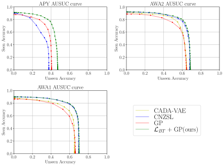
Figure 3: Comparison of Area Under Seen and Unseen Curve (AUSUC) for each dataset with CNZSL [34] and CADA-VAE [39]. Our model is performing consistently better than CNZSL and CADA-VAE on class-imbalanced datasets AWA2, AWA1 and APY.

From Figure 3 we can see that our model performs consistently better than CNZSL and CADA-VAE on class-imbalanced datasets AWA2 and APY, and competitive with CNZSL on AWA1 dataset.

IV-D Ablation Study

Model Structure Ablation: We compare our model’s performance with several similar models’ structures in Table IV. We report the performance of the Kernel Ridge Regression (KRR) model on feature space (as a baseline for GPR), KRR on latent space which is trained with our proposed $\mathcal{L}_{BT}$ loss, the Gaussian Process (GP) model on feature space and the GP model on latent space trained with the original triplet loss $\mathcal{L}_{T}$. Our model performs consistently better than all the other baseline approaches on each ZSL dataset.

Hyperparameter Ablation: We analyze the influence of two main hyperparameters on the performance of our model. These hyperparameters are the clip value that is used for preprocessing feature vectors and the threshold $\Delta$ used in triplet loss.

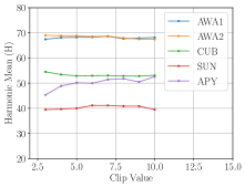
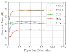
Figure 4: Harmonic mean $H$ for each dataset influenced by the hyperparameter Clip value in preprocessing (left) and $\Delta$ in triplet loss(right). Our model is stable w.r.t these hyperparameters

As can be seen from Figure 4, our model is not sensitive to the clip number that is used in data preprocessing when the clip number is in the range $[4,9]$. As long as $\Delta>3$, the performance of our model on each dataset is relatively stable.

Per-Class Accuracy Ablation: In Table V, we also provide per-class accuracy of our model $\mathcal{L}_{BT}+GP$ and traditional triplet loss $\mathcal{L}_{T}$ + GP, on unseen classes on the APY dataset. As can be seen from the table, the APY dataset has a highly class-imbalanced unseen class distribution, where 64% of the unseen test samples come from class “person”. Our model performs consistently better than traditional triplet loss models on most of the classes.

V Conclusion

In this work, we propose a novel model that combines a Neural Network and Gaussian Process regression to tackle the problems of ZSL and Generalized ZSL. We propose a NN model that projects feature vectors into a latent embedding space and generates latent prototypes of seen classes. A GP model is then trained to predict prototypes of unseen classes. Finally, a ZSL classifier is constructed using the prototypes.

We trained our NN model with a Class-Balanced Triplet loss that mitigates the problem of class imbalance in ZSL datasets. Experiments demonstrate that our model, though employing a simple design, can reach SOTA performance on the class-imbalanced ZSL datasets AWA1, AWA2 and APY in the Generalized ZSL setting.

References

- [1] M. Norouzi, T. Mikolov, S. Bengio, Y. Singer, J. Shlens, A. Frome, G. S. Corrado, and J. Dean, “Zero-shot learning by convex combination of semantic embeddings,” arXiv preprint arXiv:1312.5650, 2013.
- [2] S. Changpinyo, W.-L. Chao, B. Gong, and F. Sha, “Synthesized classifiers for zero-shot learning,” in Proceedings of the IEEE conference on computer vision and pattern recognition, 2016, pp. 5327–5336.
- [3] V. K. Verma and P. Rai, “A simple exponential family framework for zero-shot learning,” in Machine Learning and Knowledge Discovery in Databases, M. Ceci, J. Hollmén, L. Todorovski, C. Vens, and S. Džeroski, Eds. Cham: Springer International Publishing, 2017, pp. 792–808.
- [4] H. Huang, C. Wang, P. S. Yu, and C.-D. Wang, “Generative dual adversarial network for generalized zero-shot learning,” in The IEEE Conference on Computer Vision and Pattern Recognition (CVPR), June 2019.
- [5] Y. Xian, T. Lorenz, B. Schiele, and Z. Akata, “Feature generating networks for zero-shot learning,” in 2018 IEEE/CVF Conference on Computer Vision and Pattern Recognition, 2018, pp. 5542–5551.
- [6] I. J. Goodfellow, J. Pouget-Abadie, M. Mirza, B. Xu, D. Warde-Farley, S. Ozair, A. Courville, and Y. Bengio, “Generative adversarial networks,” 2014.
- [7] D. P. Kingma and M. Welling, “Auto-encoding variational bayes,” arXiv preprint arXiv:1312.6114, 2013.
- [8] Y. Le Cacheux, H. Le Borgne, and M. Crucianu, “Modeling inter and intra-class relations in the triplet loss for zero-shot learning,” in the IEEE International Conference on Computer Vision (ICCV), ser. ICCV, October 2019.
- [9] Z. Han, Z. Fu, and J. Yang, “Learning the redundancy-free features for generalized zero-shot object recognition,” in IEEE/CVF Conference on Computer Vision and Pattern Recognition (CVPR), June 2020.
- [10] S. Chen, W. Wang, B. Xia, Q. Peng, X. You, F. Zheng, and L. Shao, “Free: Feature refinement for generalized zero-shot learning,” in Proceedings of the IEEE/CVF International Conference on Computer Vision, 2021, pp. 122–131.
- [11] S. Min, H. Yao, H. Xie, C. Wang, Z. Zha, and Y. Zhang, “Domain-aware visual bias eliminating for generalized zero-shot learning,” 2020 IEEE/CVF Conference on Computer Vision and Pattern Recognition (CVPR), pp. 12 661–12 670, 2020.
- [12] Z. Han, Z. Fu, S. Chen, and J. Yang, “Contrastive embedding for generalized zero-shot learning,” in Proceedings of the IEEE/CVF Conference on Computer Vision and Pattern Recognition (CVPR), June 2021, pp. 2371–2381.
- [13] Z. Liu, Z. Miao, X. Zhan, J. Wang, B. Gong, and S. X. Yu, “Large-scale long-tailed recognition in an open world,” in IEEE Conference on Computer Vision and Pattern Recognition (CVPR), 2019.
- [14] M. Buda, A. Maki, and M. A. Mazurowski, “A systematic study of the class imbalance problem in convolutional neural networks,” Neural Networks, vol. 106, pp. 249–259, 2018.
- [15] Y. Cui, M. Jia, T.-Y. Lin, Y. Song, and S. Belongie, “Class-balanced loss based on effective number of samples,” in CVPR, 2019.
- [16] A. Farhadi, I. Endres, D. Hoiem, and D. Forsyth, “Describing objects by their attributes,” in 2009 IEEE Conference on Computer Vision and Pattern Recognition, 6 2009, pp. 1778–1785.
- [17] Y. Xian, C. H. Lampert, B. Schiele, and Z. Akata, “Zero-shot learning—a comprehensive evaluation of the good, the bad and the ugly,” IEEE Transactions on Pattern Analysis and Machine Intelligence, vol. 41, no. 9, pp. 2251–2265, Sep. 2019.
- [18] C. Rasmussen, C. Williams, M. Press, F. Bach, and P. (Firm), Gaussian Processes for Machine Learning, ser. Adaptive computation and machine learning. MIT Press, 2006. [Online]. Available: https://books.google.com.au/books?id=GhoSngEACAAJ
- [19] T. Suzuki, “Pac-bayesian bound for gaussian process regression and multiple kernel additive model,” J. Mach. Learn. Res. Wrkshp Conf. Proc., vol. 23, 01 2012.
- [20] Z. Akata, F. Perronnin, Z. Harchaoui, and C. Schmid, “Label-embedding for image classification,” IEEE transactions on pattern analysis and machine intelligence, vol. 38, no. 7, pp. 1425–1438, 2015.
- [21] J. Snell, K. Swersky, and R. S. Zemel, “Prototypical networks for few-shot learning,” in NIPS, 2017.
- [22] R. Boney and A. Ilin, “Semi-supervised few-shot learning with prototypical networks,” CoRR abs/1711.10856, 2017.
- [23] T. Gao, X. Han, Z. Liu, and M. Sun, “Hybrid attention-based prototypical networks for noisy few-shot relation classification,” in Proceedings of the AAAI Conference on Artificial Intelligence, vol. 33, 2019, pp. 6407–6414.
- [24] O. Chapelle, B. Scholkopf, and E. A. Zien, “Semi-supervised learning (chapelle, o. et al., eds.; 2006) [book reviews],” vol. 20, no. 3, pp. 542–542, 2009.
- [25] K. Li, M. R. Min, and Y. Fu, “Rethinking zero-shot learning: A conditional visual classification perspective,” in Proceedings of the IEEE International Conference on Computer Vision, 2019, pp. 3583–3592.
- [26] Y. Meng and Y. Guo, “Zero-shot classification with discriminative semantic representation learning,” in 2017 IEEE Conference on Computer Vision and Pattern Recognition (CVPR), 2017.
- [27] Y. Wen, K. Zhang, Z. Li, and Y. Qiao, “A discriminative feature learning approach for deep face recognition,” in European conference on computer vision. Springer, 2016, pp. 499–515.
- [28] Y. Dolma and V. P. Namboodiri, “Using gaussian processes to improve zero-shot learning with relative attributes,” in Computer Vision – ACCV 2016, S.-H. Lai, V. Lepetit, K. Nishino, and Y. Sato, Eds. Cham: Springer International Publishing, 2017, pp. 150–164.
- [29] T. Mukherjee and T. Hospedales, “Gaussian Visual-Linguistic Embedding for Zero-Shot Recognition,” in Proceedings of the 2016 Conference on Empirical Methods in Natural Language Processing. Austin, Texas: Association for Computational Linguistics, Nov. 2016, pp. 912–918. [Online]. Available: https://www.aclweb.org/anthology/D16-1089
- [30] M. Elhoseiny, B. Saleh, and A. Elgammal, “Write a classifier: Zero-shot learning using purely textual descriptions,” in Proceedings of the IEEE International Conference on Computer Vision, 2013, pp. 2584–2591.
- [31] C. Huang, Y. Li, C. C. Loy, and X. Tang, “Deep imbalanced learning for face recognition and attribute prediction,” IEEE transactions on pattern analysis and machine intelligence, vol. 42, no. 11, pp. 2781–2794, 2019.
- [32] K. Sohn, “Improved deep metric learning with multi-class n-pair loss objective,” in Advances in Neural Information Processing Systems, D. Lee, M. Sugiyama, U. Luxburg, I. Guyon, and R. Garnett, Eds., vol. 29. Curran Associates, Inc., 2016.
- [33] Y. Le Cacheux, H. Le Borgne, and M. Crucianu, “From classical to generalized zero-shot learning: A simple adaptation process,” in International Conference on Multimedia Modeling. Springer, 2019, pp. 465–477.
- [34] I. Skorokhodov and M. Elhoseiny, “Class normalization for (continual)? generalized zero-shot learning,” in Proceedings of the International Conference on Learning Representations (ICLR), 2021.
- [35] C. Wah, S. Branson, P. Welinder, P. Perona, and S. Belongie, “The Caltech-UCSD Birds-200-2011 Dataset,” California Institute of Technology, Tech. Rep. CNS-TR-2011-001, 2011.
- [36] G. Patterson and J. Hays, “Sun attribute database: Discovering, annotating, and recognizing scene attributes,” in 2012 IEEE Conference on Computer Vision and Pattern Recognition. IEEE, 2012, pp. 2751–2758.
- [37] A. Frome, G. S. Corrado, J. Shlens, S. Bengio, J. Dean, M. Ranzato, and T. Mikolov, “Devise: A deep visual-semantic embedding model,” in Advances in neural information processing systems, 2013, pp. 2121–2129.
- [38] Z. Yue, T. Wang, H. Zhang, Q. Sun, and X. Hua, “Counterfactual zero-shot and open-set visual recognition,” CoRR, vol. abs/2103.00887, 2021. [Online]. Available: https://arxiv.org/abs/2103.00887
- [39] E. Schönfeld, S. Ebrahimi, S. Sinha, T. Darrell, and Z. Akata, “Generalized zero- and few-shot learning via aligned variational autoencoders,” in 2019 IEEE/CVF Conference on Computer Vision and Pattern Recognition (CVPR), 2019, pp. 8239–8247.
- [40] S. Narayan, A. Gupta, F. S. Khan, C. G. Snoek, and L. Shao, “Latent embedding feedback and discriminative features for zero-shot classification,” in ECCV, 2020.
- [41] J. Li, M. Jing, K. Lu, Z. Ding, L. Zhu, and Z. Huang, “Leveraging the invariant side of generative zero-shot learning,” in Proceedings of the IEEE/CVF Conference on Computer Vision and Pattern Recognition, 2019, pp. 7402–7411.
- [42] Y. Yu, Z. Ji, J. Han, and Z. Zhang, “Episode-based prototype generating network for zero-shot learning,” in IEEE/CVF Conference on Computer Vision and Pattern Recognition (CVPR), June 2020.
- [43] J. R. Gardner, G. Pleiss, D. Bindel, K. Q. Weinberger, and A. G. Wilson, “Gpytorch: Blackbox matrix-matrix gaussian process inference with gpu acceleration,” arXiv preprint arXiv:1809.11165, 2018.
- [44] D. P. Kingma and J. Ba, “Adam: A method for stochastic optimization,” in 3rd International Conference on Learning Representations, ICLR 2015, San Diego, CA, USA, May 7-9, 2015, Conference Track Proceedings, Y. Bengio and Y. LeCun, Eds., 2015. [Online]. Available: http://arxiv.org/abs/1412.6980
- [45] Y. Xian, S. Sharma, B. Schiele, and Z. Akata, “F-vaegan-d2: A feature generating framework for any-shot learning,” in 2019 IEEE/CVF Conference on Computer Vision and Pattern Recognition (CVPR), 2019, pp. 10 267–10 276.
- [46] F. Sung, Y. Yang, L. Zhang, T. Xiang, P. H. S. Torr, and T. M. Hospedales, “Learning to compare: Relation network for few-shot learning,” in 2018 IEEE/CVF Conference on Computer Vision and Pattern Recognition, 2018, pp. 1199–1208.
- [47] D. Huynh and E. Elhamifar, “Fine-grained generalized zero-shot learning via dense attribute-based attention,” in IEEE/CVF Conference on Computer Vision and Pattern Recognition (CVPR), June 2020.
- [48] R. Keshari, R. Singh, and M. Vatsa, “Generalized zero-shot learning via over-complete distribution,” in IEEE/CVF Conference on Computer Vision and Pattern Recognition (CVPR), June 2020.
- [49] Y. Shen, J. Qin, L. Huang, L. Liu, F. Zhu, and L. Shao, “Invertible zero-shot recognition flows,” in European Conference on Computer Vision, 2020, pp. 614–631.
- [50] Y.-Y. Chou, H.-T. Lin, and T.-L. Liu, “Adaptive and generative zero-shot learning,” in International Conference on Learning Representations, 2020.
- [51] L. Liu, T. Zhou, G. Long, J. Jiang, X. Dong, and C. Zhang, “Isometric propagation network for generalized zero-shot learning,” in International Conference on Learning Representations, 2020.
- [52] M. Kampffmeyer, Y. Chen, X. Liang, H. Wang, Y. Zhang, and E. P. Xing, “Rethinking knowledge graph propagation for zero-shot learning,” in 2019 IEEE/CVF Conference on Computer Vision and Pattern Recognition (CVPR), 2019, pp. 11 487–11 496.
- [53] S. Liu, J. Chen, L. Pan, C.-W. Ngo, T.-S. Chua, and Y.-G. Jiang, “Hyperbolic visual embedding learning for zero-shot recognition,” in 2020 IEEE/CVF Conference on Computer Vision and Pattern Recognition (CVPR), 2020, pp. 9273–9281.
- [54] J. Wu, T. Zhang, Z.-J. Zha, J. Luo, Y. Zhang, and F. Wu, “Self-supervised domain-aware generative network for generalized zero-shot learning,” in 2020 IEEE/CVF Conference on Computer Vision and Pattern Recognition (CVPR), 2020, pp. 12 767–12 776.