Fast Bayesian Updates for Deep Learning with a Use Case in Active Learning

Abstract

Retraining deep neural networks when new data arrives is typically computationally expensive. Moreover, certain applications do not allow such costly retraining due to time or computational constraints. Fast Bayesian updates are a possible solution to this issue. Therefore, we propose a Bayesian update based on Monte-Carlo samples and a last-layer Laplace approximation for different Bayesian neural network types, i.e., Dropout, Ensemble, and Spectral Normalized Neural Gaussian Process (SNGP). In a large-scale evaluation study, we show that our updates combined with SNGP represent a fast and competitive alternative to costly retraining. As a use case, we combine the Bayesian updates for SNGP with different sequential query strategies to exemplarily demonstrate their improved selection performance in active learning.

1 Introduction

Extending a dataset with new samples to train a deep learning model typically poses two problems. Updating a trained model may cause catastrophic forgetting while retraining may require high computational effort. Although the generalization performance typically justifies exhaustive retraining procedures, in some applications, retraining is not possible due to, for example, (1) the high number of retraining procedures in applications where data arrives sequentially and immediate updates are beneficial, e.g., in active learning (Settles, 2009) or when working on data streams (Sahoo et al., 2018), (2) the lack of computational power, e.g., for execution on embedded hardware (Taylor et al., 2018), (3) privacy reasons, e.g., when new data cannot be sent to distributed computing units (Taylor et al., 2018). Therefore, we suggest using Bayesian neural networks (BNNs, Fortuin, 2022) in the above examples as they not only provide additional uncertainty estimates or out-of-distribution detection capabilities but also allow updating the predictions with additional data without retraining the network (Kirsch et al., 2022).

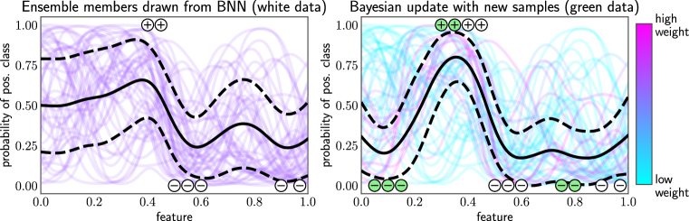
Figure 1: The left plot shows the predicted probabilities of the positive class for each ensemble member (colored lines) drawn from a BNN as well as the mean (black solid line) and standard deviation (black dashed line) of its predictive distribution. The right plot shows updated weights for each ensemble member and the predictive distribution after observing additional samples (green).

In this article, we develop a fast Bayesian update algorithm for BNNs. Figure 1 (left) shows the idea of sampling an ensemble of probabilistic hypotheses, each representing a possible true solution for the learning task (white samples). When new data (green samples) comes in, we weigh each ensemble member by its likelihood of explaining the new data and obtain an updated ensemble without retraining the BNN. This results in an updated predictive distribution, as seen in bold in Fig. 1 (right). We apply this general idea for different BNN types, i.e., Monte-Carlo-based (MC-based) Dropout, (Deep) Ensembles, and last-layer Laplace approximations (LA) (Ritter et al., 2018a) via Spectral Normalized Neural Gaussian Process (SNGP, Liu et al., 2020). In contrast to Dropout and Ensembles, SNGP allows for fast Bayesian updates without the need to sample ensemble members.

Active learning (Settles, 2009) provides an interesting use case for our Bayesian update approach. Here, a query strategy iteratively selects unlabeled samples to be labeled by an oracle. This selection is based on information provided by a model trained on the currently available labeled samples. The goal is to maximize the model’s performance while minimizing the number of label acquisitions. In deep learning settings, samples are typically chosen in batches to reduce the number of retraining processes after the selection step (Kirsch et al., 2019). BNNs, together with our Bayesian updates, do not require batch strategies and can immediately make use of use the new labels.

Our research question and contributions are as follows: How can we efficiently update BNNs, and which aspects influence the quality of such updates?

• We propose a fast Bayesian update algorithm for BNNs based on MC sampling (Ensemble, Dropout) and a last-layer LA (SNGP).

• We evaluate the investigated BNNs and their potential for Bayesian updates regarding their generalization performance, probability calibration, and out-of-distribution detection, and we hypothesize why SNGP outperforms its competitors.

• We show the effectiveness of using sequential Bayesian updates for selecting diverse sample batches in an active learning use case with SNGP for several existing query strategies.

2 Related Work

Here, we discuss related work regarding the two main parts of our proposed Bayesian update: BNNs and corresponding update approaches. Furthermore, we briefly review deep active learning literature.

Bayesian neural networks (Wang & Yeung, 2020; Fortuin, 2022) induce a prior distribution over their parameters, i.e., weights, and learn a posterior distribution for given training data. Predictions are then made by marginalizing over this posterior distribution. BNN types differ mainly in their assumed probabilistic model and the sampling of the posterior distribution (Jospin et al., 2022). Gal & Ghahramani (2016) proposed (MC-)Dropout as one of the most prominent BNN types. Usually, Dropout is a regularization technique performed during training. Using Dropout during evaluation, we obtain a distribution for the predictions corresponding to a variational distribution in the parameter space. Due to Dropout’s simplicity and efficiency, it is often used for comparison. However, its predictions may not properly represent uncertainty estimates (Ovadia et al., 2019). (Deep) Ensembles (Lakshminarayanan et al., 2017), another prominent BNN type, consist of multiple point-estimate neural networks. Combined with regularization, these different point estimates approximate modes of the parameters’ posterior distribution. Ensembles typically provide better uncertainty estimates than Dropout but require significantly more computational capacity during training (Ovadia et al., 2019). A BNN obtained via LA (Ritter et al., 2018b) can be seen as a trade-off between Dropout and Ensembles regarding computational requirements. It specifies a Gaussian posterior distribution, where the maximum a posteriori (MAP) estimate defines the mean and the inverse of the negative log likelihood’s Hessian corresponds to the covariance matrix. As computing this Hessian is expensive for large networks, LA is often used only in the last layer (Daxberger et al., 2021). SNGP (Liu et al., 2020) follows this line of work together with random Fourier features (Rahimi & Recht, 2007) and spectral normalization (Miyato et al., 2018) to approximate a Gaussian process providing distance-aware uncertainty estimates.

Updating neural networks is closely related to online (Hoi et al., 2021) and continual learning (De Lange et al., 2021), where a model learns from sequentially arriving samples. Recent approaches, such as elastic weight consolidation (Kirkpatrick et al., 2017) and online LA (Ritter et al., 2018a), demonstrated how updates can be performed for BNNs. Due to the lack of a closed form for updating the posterior over a BNN’s parameters, they use gradient-based methods. Our proposed Bayesian update for SNGP is highly related to online LA. However, our update only considers the last layer of SNGP. Therefore, we adapt the ideas of (Spiegelhalter & Lauritzen, 1990), which allow fast updating via second-order optimization algorithms. Similar to Kirsch et al. (2022), we are not only interested in overcoming catastrophic forgetting by achieving high accuracy on old and new data samples but additionally investigate gains of updates regarding various performance types, e.g., out-of-distribution detection (Yang et al., 2021) and probability calibration (Guo et al., 2017).

Deep active learning strategies need to select batches of samples to reduce the number of networks’ retraining procedures (Ren et al., 2021). The most simple batch selection scheme, referred to as top-$b$ selection, employs a sequential query strategy for computing sample-wise utility scores and selects a predefined number of samples with the highest scores. This way, we can directly transform sequential strategies such as Uncertainty Sampling (US, Lewis & Catlett, 1994) and Query-by-Committee (QBC, Seung et al., 1992) into batch strategies. For an improved information-theoretic selection, these kinds of query strategies are mostly used in combination with BNNs, such as Dropout for Bayesian Active Learning by Disagreement (BALD, Gal et al., 2017) and Ensemble for Variation Ratio (Beluch et al., 2018). However, a top-$b$ selection ignores the samples’ diversity in a batch. Therefore, several other query strategies have been proposed, e.g., BatchBALD (Kirsch et al., 2019) for BNNs or CoreSet (Sener & Savarese, 2018) for deterministic networks, explicitly modeling sample diversity in a batch.

3 Fast Bayesian Updates for Bayesian Neural Networks

Here, we present two approximations of Bayesian updates (MC- and LA-based) for Ensembles, Dropout, and SNGP as three different BNN types to be employed in online learning tasks. For detailed explanations of all models, we refer to Appendix C.

3.1 Bayesian Updates

In this section, we present the details of how to incorporate the information of new sample-label pairs ${\mathcal{D}^{\oplus}=\{(\bm{x}_{1},y_{1}),\dots,(\bm{x}_{N},y_{N})\}\subset\mathcal{X}\times\mathcal{Y}}$ into a BNN trained on a dataset $\mathcal{D}\subset\mathcal{X}\times\mathcal{Y}$ via Bayesian updates. We focus on classification problems with labels $\mathcal{Y}=\{0,\dots,K-1\}$. Our goal is to use this new data for updating the probabilistic predictions, i.e., computing $p(y|\bm{x},\mathcal{D}^{\oplus}\cup\mathcal{D})$. Retraining the entire network on the extended data set $\mathcal{D}^{\oplus}\cup\mathcal{D}$ results in high computational cost for a large dataset $\mathcal{D}$, even if only the last layer is retrained. Using the new data solely, catastrophic forgetting can lead to overfitting and is challenging to be overcome (Ritter et al., 2018a).

We propose to employ techniques of Bayesian deep learning (Fortuin, 2022) in a new combination with Bayesian online learning (Opper & Winther, 1999) as an efficient and effective alternative for updating a BNN’s prediction. The main idea of Bayesian deep learning is to estimate a posterior distribution $p(\bm{\omega}|\mathcal{D})$ over a BNN’s parameters $\bm{\omega}\in\mathrm{\Omega}$ given the observed training data $\mathcal{D}$ by using Bayes’ theorem. The obtained posterior distribution over the parameters can then be used to specify the predictive distribution over a new sample’s class membership via marginalization:

$$p(y|\bm{x},\mathcal{D})=\operatorname*{\mathbb{E}}_{\bm{\omega}|\mathcal{D}}\Big{[}p(y|\bm{x},\bm{\omega})\Big{]}=\int p(y|\bm{x},\bm{\omega})p(\bm{\omega}|\mathcal{D})\mathop{}\!\mathrm{d}\bm{\omega}.$$ (1)

Thereby, the distribution $p(y|\bm{x},\bm{\omega})$ denotes the probabilistic output of a network with parameters $\bm{\omega}$:

$$p(y|\bm{x},\bm{\omega})=[\mathrm{softmax}(\bm{f}_{\bm{\omega}}(\bm{x}))]_{y}=\frac{\exp([\bm{f}_{\bm{\omega}}(\bm{x})]_{y})}{\sum_{y^{\prime}\in\mathcal{Y}}\exp([\bm{f}_{\bm{\omega}}(\bm{x})]_{y^{\prime}})},$$ (2)

where $\bm{f}_{\bm{\omega}}:\mathcal{X}\rightarrow\mathbb{R}^{K}$ represents a network as a function outputting class-wise logits. Since the probabilistic outputs in Eq. (2) are not directly dependent on the training data $\mathcal{D}$, we only need to update the distribution over the parameters for updating the BNN’s predictive distribution. As samples in $\mathcal{D}$ and $\mathcal{D}^{\oplus}$ are assumed to be independently distributed, we can simplify the likelihood in Bayes’ theorem and reformulate the parameter distribution as follows:

$$p(\bm{\omega}|\mathcal{D}^{\oplus}\cup\mathcal{D})\propto p(\bm{\omega}|\mathcal{D})p(\mathcal{D}^{\oplus}|\mathcal{D},\bm{\omega})=p(\bm{\omega}|\mathcal{D})p(\mathcal{D}^{\oplus}|\bm{\omega})=p(\bm{\omega}|\mathcal{D})\prod_{(\bm{x},y)\in\mathcal{D}^{\oplus}}p(y|\bm{x},\bm{\omega}).$$ (3)

As a result, the updated parameter distribution $p(\bm{\omega}|\mathcal{D}^{\oplus}\cup\mathcal{D})$ is found by combining the current posterior distribution $p(\bm{\omega}|\mathcal{D})$ with the incoming likelihood $p(y|\bm{x},\bm{\omega})$ per sample-label pair $(\bm{x},y)\in\mathcal{D}^{\oplus}$. We refer to Eq. (3) as the Bayesian update and present approximations for specific BNNs next.

3.2 Fast Approximations of Bayesian Updates for Deep BNNs

In this section, we propose a general approximation of Bayesian updates based on MC sampling and a more specific approximation for BNNs utilizing a last-layer LA (e.g., SNGP).

MC-based Bayesian Updates: BNNs such as Ensembles and Dropout allow drawing samples from the posterior distribution $p(\bm{\omega}|\mathcal{D})$. More precisely, Ensembles train multiple randomly initialized networks, while Dropout randomly sets a predefined portion of parameters to zero for multiple inference steps to obtain samples. For MC-based approaches, we assume that every ensemble member $\bm{\omega}_{m}\sim p(\bm{\omega}|\mathcal{D})$ is drawn with equal probability. Hence, we initialize the approximate distribution over the drawn members by categorical distribution with parameters $\bm{\hat{p}}={(\hat{p}_{1},\ldots,\hat{p}_{M})}^{\mathrm{T}}$:

$$q(\bm{\omega}_{m}|\mathcal{D})=\operatorname{Cat}(m|\bm{\hat{p}})=\hat{p}_{m}=\nicefrac{{1}}{{M}},$$ (4)

where $M$ is the number of drawn ensemble members. We approximate the updated posterior distribution, which includes our new dataset $\mathcal{D}^{\oplus}$, by using Eq. (3) accordingly:

$$q(\bm{\omega}_{m}|\mathcal{D}^{\oplus}\cup\mathcal{D})=\operatorname{Cat}(m|\bm{\hat{p}}^{\mathrm{upd}}) \propto q(\bm{\omega}_{m}|\mathcal{D})\prod_{(\bm{x},y)\in\mathcal{D}^{\oplus}}p(y|\bm{x},\bm{\omega}_{m})$$ (5)

$$=\hat{p}_{m}\prod_{(\bm{x},y)\in\mathcal{D}^{\oplus}}\left[\mathrm{softmax}(\bm{f}_{\bm{\omega}_{m}}(\bm{x}))\right]_{y}=\hat{z}_{m},$$ (6)

which is also a categorical distribution with parameters $\bm{\hat{p}}^{\mathrm{upd}}={(\hat{p}_{1}^{\mathrm{upd}},\ldots,\hat{p}_{M}^{\mathrm{upd}})}^{\mathrm{T}}$ that we obtain after normalizing $\bm{\hat{z}}={(\hat{z}_{1},\ldots,\hat{z}_{M})}^{\mathrm{T}}$. Intuitively, the importance of each ensemble member is determined by its likelihood of explaining the new dataset $\mathcal{D}^{\oplus}$.

The discrete approximation $q(\bm{\omega}_{m}|\mathcal{D}^{\oplus}\cup\mathcal{D})$ of the updated posterior distribution allows us to make new predictions (see Eq. (1)) by evaluating

$$p(y|\bm{x},\mathcal{D}^{\oplus}\cup\mathcal{D})=\operatorname*{\mathbb{E}}_{\bm{\omega}|\mathcal{D}^{\oplus}\,\cup\,\mathcal{D}}\Big{[}p(y|\bm{x},\bm{\omega})\Big{]} \approx\sum_{m=1}^{M}p(y|\bm{x},\bm{\omega}_{m})\cdot q(\bm{\omega}_{m}|\mathcal{D}^{\oplus}\cup\mathcal{D})$$ (7)

$$=\sum_{m=1}^{M}\left[\mathrm{softmax}(\bm{f}_{\bm{\omega}_{m}}(\bm{x}))\right]_{y}\cdot\hat{p}_{m}^{\mathrm{upd}}.$$ (8)

LA-based Bayesian Updates: In the following, we focus on binary classification with $K=2$ and refer to Appendix A for an extension to multi-class classification. SNGP learns a distance preserving hidden mapping via spectral normalization as the output of the penultimate layer. By transforming these outputs with a random Fourier feature mapping (Rahimi & Recht, 2007), we obtain a $D$-dimensional representation $\bm{\phi}(\bm{x})\in\mathbb{R}^{D}$ (for a rationale see Appendix C.3). A last-layer LA is then performed on $\bm{\phi}(\bm{x})$ via a multivariate normal distribution over the parameters $\bm{\omega}\in\mathbb{R}^{D}$:

$$q(\bm{\omega}|\mathcal{D})=\operatorname{\mathcal{N}}(\bm{\omega}|\bm{\hat{\mu}},\bm{\hat{\Sigma}}) \propto q(\bm{\omega})\prod_{(\bm{x},y)\in\mathcal{D}}p(y|\bm{x},\bm{\omega})\quad\text{with prior}\quad q(\bm{\omega})=\operatorname{\mathcal{N}}(\bm{\omega}|\bm{0},\lambda^{-1}\bm{I}).$$ (9)

SNGP computes the mean $\bm{\hat{\mu}}\in\mathbb{R}^{D}$ as the MAP estimate on $\mathcal{D}$ with gradient optimization and weight decay $\lambda\in\mathbb{R}_{>0}$. The covariance matrix $\bm{\hat{\Sigma}}=\bm{H}^{-1}(\bm{\hat{\mu}},\lambda^{-1}\bm{I},\mathcal{D})\in\mathbb{R}^{D\times D}$ can then be calculated as the inverse Hessian matrix of the negative log posterior likelihood evaluated at the MAP estimate $\bm{\hat{\mu}}$ given training data $\mathcal{D}$ and the covariance matrix of the prior $\lambda^{-1}\bm{I}$. For any mean $\bm{\mu}$, covariance matrix $\bm{\Sigma}$, and dataset $\mathcal{A}$, we compute the inverse Hessian following Spiegelhalter & Lauritzen (1990):

$$\bm{H}^{-1}(\bm{\mu},\bm{\Sigma},\mathcal{A}) =\bm{\Sigma}-\sum_{(\bm{x},y)\in\mathcal{A}}\frac{g\big{(}\bm{\phi}(\bm{x}),\bm{\mu}\big{)}}{1+{\bm{\phi}(\bm{x})}^{\mathrm{T}}\bm{\Sigma}\bm{\phi}(\bm{x})\,g\big{(}\bm{\phi}(\bm{x}),\bm{\mu}\big{)}}\big{(}\bm{\Sigma}\bm{\phi}(\bm{x})\big{)}{\big{(}\bm{\Sigma}\bm{\phi}(\bm{x})\big{)}}^{\mathrm{T}}$$ (10)

$$\text{with }g(\bm{\phi}(\bm{x}),\bm{\mu}) =\sigma({\bm{\phi}(\bm{x})}^{\mathrm{T}}{\bm{\mu}})(1-\sigma({\bm{\phi}(\bm{x})}^{\mathrm{T}}{\bm{\mu}}))\text{ and }\sigma(x)=(1+\exp(-x))^{-1}.$$ (11)

When observing new data, we follow the same idea as in Eq. 9 with $q(\bm{\omega}|\mathcal{D})$ as our new prior:

$$q(\bm{\omega}|\mathcal{D}\cup\mathcal{D}^{\oplus}) \propto q(\bm{\omega}|\mathcal{D})\prod_{(\bm{x},y)\in\mathcal{D}^{\oplus}}p(y|\bm{x},\bm{\omega})\approx\operatorname{\mathcal{N}}(\bm{\omega}|\bm{\hat{\mu}}^{\mathrm{upd}},\bm{\hat{\Sigma}}^{\mathrm{upd}}).$$ (12)

In accordance with Spiegelhalter & Lauritzen (1990), we implement the updates based on the Gauss-Newton algorithm:

$$\bm{\hat{\mu}}^{\mathrm{upd}} =\bm{\hat{\mu}}-\bm{H}^{-1}(\bm{\hat{\mu}},\bm{\hat{\Sigma}},\mathcal{D}^{\oplus})\sum_{(\bm{x},y)\in\mathcal{D}^{\oplus}}\Big{(}\sigma\big{(}{\bm{\phi}(\bm{x})}^{\mathrm{T}}{\bm{\hat{\mu}}}\big{)}-y\Big{)}\bm{\phi}(\bm{x}),$$ (13)

$$\bm{\hat{\Sigma}}^{\mathrm{upd}} =\bm{H}^{-1}(\bm{\hat{\mu}}^{\mathrm{upd}},\bm{\hat{\Sigma}},\mathcal{D}^{\oplus}).$$ (14)

As we only update the last layer, we can use such a second-order algorithm that provides more robust estimates than (first-order) stochastic gradient optimization and can also be repeated multiple times. Following Liu et al. (2020), we make predictions by considering the mean-field approximation on the updated normal distribution with $c=\nicefrac{{\pi}}{{8}}$ (Bishop, 2006) according to:

$$p(y=1|\bm{x},\mathcal{D}\cup\mathcal{D}^{\oplus}) \approx\sigma\left(\frac{{\bm{\phi}(\bm{x})}^{\mathrm{T}}\,\bm{\hat{\mu}}^{\mathrm{upd}}}{\sqrt{1+c\cdot{\bm{\phi}(\bm{x})}^{\mathrm{T}}\,\bm{\hat{\Sigma}}^{\mathrm{upd}}\,\bm{\phi}(\bm{x})}}\right).$$ (15)

4 Bayesian Updating Experiments

In this section, we evaluate MC- and LA-based Bayesian updates in comparison to retraining a BNN. Further, we identify concrete aspects influencing the quality of such updates.

4.1 Experimental Setup

Our experimental design follows the work of Kirsch et al. (2022). First, we train a BNN on the training dataset $\mathcal{D}$ (baseline). We then use this baseline BNN to perform Bayesian updates on additional sample-label pairs $\mathcal{D}^{\oplus}$ and compare these results to retraining the entire BNN from scratch on the overall dataset $\mathcal{D}\cup\mathcal{D}^{\oplus}$. We perform such an experiment for varying sizes of the training dataset, i.e., $|\mathcal{D}|\in\{16,32,\dots,320\}$, and a fixed size of new sample-label pairs, i.e., $|\mathcal{D}^{\oplus}|=32$. Thus, we can evaluate the impact of Bayesian updates in different learning stages. For reasons of reproducibility, we repeat each experiment 10 times and publish our code on https://github.com/ies-research/bayesian-updates.

Table 1: Overview of datasets.

Type	Dataset	Reference	# classes	# features
Tabular	LETTER	Frey & Slate (1991)	26	16
	PDIGITS	Dua & Graff (2017)	10
Image	MNIST	LeCun & Cortes (1998)	10	28 $\times$ 28
	FMNIST	Xiao et al. (2017)

The datasets $\mathcal{D}$ and $\mathcal{D}^{\oplus}$ are randomly sampled from real-world datasets. We use two tabular and two image benchmark datasets from literature. Table 1 summarizes further information. For visualization, we experiment on the two-dimensional toy dataset TWO-MOONS as shown in Fig. 2.

Typically, the selection of performance metrics depends on the application at hand, whereas we aim to evaluate the Bayesian updates as generically as possible here. For this reason, we investigate three performance aspects being of interest in several applications: (1) generalization performance measured via accuracy (ACC, to be maximized $\uparrow$), (2) uncertainty estimation capabilities measured via area under receiver operation characteristic (AUROC, to be maximized $\uparrow$) curve in an out-of-distribution (OOD) detection scenario, and (3) probability calibration measured via negative log-likelihood (NLL, to be minimized $\downarrow$). The ACC and NLL scores are computed on a fixed test set obtained after a predefined train-test-split of the respective dataset. For the OOD detection task, we need an OOD dataset which is PDIGITS for LETTER (and vice versa) and FMNIST for MNIST (and vice versa). We compute two types of scores for classifying samples as in- or out-of-distribution from which we calculate the AUROC, namely, the entropy of the predictive distribution and the mean variance over the distribution of predicted class membership probabilities. Both scores are expected to be high if a sample has a high likelihood of being out-of-distribution. We refer to Appendix B for further details.

Our evaluation focuses on Ensemble, Dropout, and SNGP as three common BNN types. Ensemble and Dropout can only be evaluated with the MC-based update and inference scheme. For SNGP, we evaluate SNGP-MC in the same manner, while SNGP-LA uses the LA-based update and the mean-field approximation for inference. Their network architectures and hyperparameters are selected in dependence of the respective dataset. We implement a multilayer perceptron with two residual blocks as base architecture for the two tabular datasets and the toy dataset, while we use a ResNet-6 architecture for the two image datasets. An Ensemble consists of 20 independently trained and randomly initialized base architectures. In each residual block of the Dropout networks, we add a Dropout layer with a rate of 50$\%$ in the multilayer perceptron architecture and 20$\%$ in the ResNet-6 architecture. For updating and inference, Dropout uses 1000 ensemble members. SNGP is implemented for both architectures by applying spectral normalization to the hidden layers and a random Fourier feature mapping to the penultimate layer’s outputs. Since SNGP-MC uses an efficient last-layer LA, it uses 20000 ensemble members for its updates and inference. Appendix C summarizes further hyperparameters and design choices for each BNN. The hyperparameters’ influence is investigated in our ablation study in Appendix D.

4.2 Results

The presentation of our results is threefold: (1) we visualize and discuss the behavior of our Bayesian updates on the two-dimensional toy dataset, (2) we present performance difference curves for the real-world datasets to get an understanding of the impact of Bayesian updates at different learning stages, and (3) we give a compact tabular overview of all obtained results.

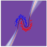
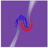
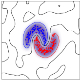
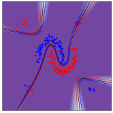
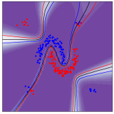
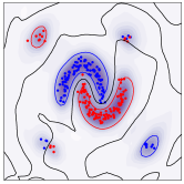
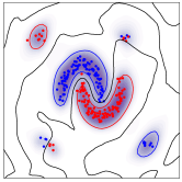
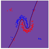
(a) Ensemble

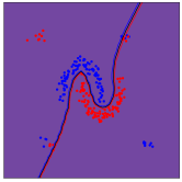
(b) Dropout

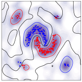
(c) SNGP-MC

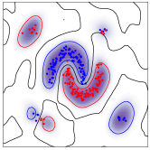
(d) SNGP-LA

Figure 2: Visualization of the predictive distribution’s mean and variance for Ensemble, Dropout, SNGP-MC, and SNGP-LA as BNNs after (re)training and Bayesian updating on a two-dimensional toy dataset.

1. Behavior Visualization: Fig. 2 visualizes the results for the two-dimensional toy dataset TWO-MOONS. There are samples of two classes represented by the blue and red colored circles. The columns refer to the four evaluated BNNs. The upper row shows the baseline BNNs trained on $\mathcal{D}$ consisting of two moons in the center. In the second row, we see the BNNs retrained on the moons and four new clusters (corresponding to the extended training set $\mathcal{D}\cup\mathcal{D}^{\oplus}$). The third row gives an overview of the BNNs obtained after applying the Bayesian updates for the new clusters in $\mathcal{D}^{\oplus}$. The predictive distribution of each of these BNNs is plotted as contour lines, where the red/blue lines show 70% probability for the red/blue class, while the black lines represent the 50$\%$ decision boundary. Each plot’s background shows the mean variance over the predicted class membership probabilities as proxies for the BNNs’ epistemic uncertainty. A high epistemic uncertainty corresponds to missing knowledge of the BNN. The quality of this uncertainty is often evaluated via additional out-of-distribution samples, for which the BNN should return high uncertainty estimates.

Comparing the four baseline BNNs, we observe that each BNN can accurately separate the two moons. However, only SNGP-MC and SNGP-LA also model high variance, i.e., diverse probabilistic hypotheses, in regions without observed training data. In contrast, Ensemble and Dropout only model different probabilistic hypotheses close to their decision boundaries only. These observations are still valid after retraining the BNNs on $\mathcal{D}\cup\mathcal{D}^{\oplus}$ (second row). Inspecting the BNNs with Bayesian updates (third row), we see that the BNNs of Dropout and Ensemble cannot correctly adjust their class predictions for the additional clusters due to missing diversity in the probabilistic hypotheses (ensemble members). Moreover, we observe low variances in the entire feature space, which results from assigning a weight near one to a single ensemble member. In comparison, Bayesian updating for SNGP-MC and SNGP-LA works nearly as good as retraining: The predictions are correctly learned for newly added data without any catastrophic forgetting regarding the original training data. Also, the quality of the variance, which models epistemic uncertainty, is preserved. Thereby, the MC-based Bayesian update is slightly less robust than the LA-based Bayesian update.

2. Performance Difference Curves: Fig. 3 shows the results of Bayesian updates, compared to retraining with respect to the number of samples in $\mathcal{D}$. Therefore, we start with $|\mathcal{D}|\in\{\mbox{16, 32, \ldots, 320}\}$ samples ($x$-axis) for training the baseline BNN, then add 32 randomly selected samples in $\mathcal{D}^{\oplus}$ for either updating with $\mathcal{D}^{\oplus}$ or retraining with $\mathcal{D}\cup\mathcal{D}^{\oplus}$, and compute their performance differences regarding ACC, NLL, and AUROC ($y$-axis) to this baseline BNN (dashed line). In Fig. 3, we plot the retrained BNNs as semi-transparent lines, and the Bayesian updated BNNs as solid lines with circles. In general, we observe that retraining a BNN from scratch is superior to Bayesian updating in terms of ACC improvement. Thereby, the impact of retraining and Bayesian updates decreases with an increasing size of $\mathcal{D}$. Comparing the individual BNNs, we further see that the Bayesian updates work only for SNGP. Specifically, SNGP-LA improves the ACC compared to its baseline across all four datasets, while SNGP-MC fails for the LETTER dataset. A possible explanation could be a more complex space of probabilistic hypotheses due to a higher number of classes for this dataset. Another observation is that the ACC improvements of Bayesian updates are higher for the tabular than the image datasets. Likely, this observation results from the higher importance of feature learning in the hidden layers for the image datasets. The other performance metrics AUROC and NLL, shown for the MNIST dataset, confirm the improvements of Bayesian updates for SNGP. The other plots are given in Appendix E.

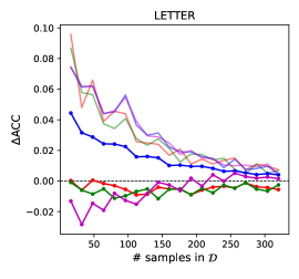
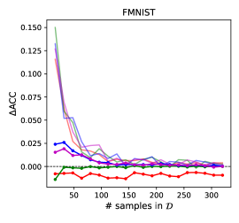
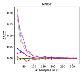
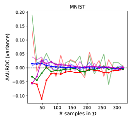
Figure 3: Performance difference curves for four benchmark datasets showing performance differences of retrained and updated BNNs compared to their respective baseline BNN for different training set sizes and performance metrics.

3. Tabular Results: For a more compact overview, Table 2 summarizes the performance difference curves in Fig. 3 through averaging over the different sample sizes in the baseline BNN’s training dataset. For reference, we also report the averaged absolute performance of the baseline BNN for each dataset, performance metric, and BNN type. The symbol ^∗ indicates a significant performance improvement between the baseline and its Bayesian updated/retrained BNN according to a one-sided t-test conducted with a p-value of 0.01 over ten repetitions. We additionally report the computation times (TIME [s]) of an NVIDIA GPU A100 for evaluating the efficiency of retraining, Bayesian updates, and predictions with respect to the four evaluated BNNs.

Table 2: Overview of averaged absolute baseline performances, their relative performance differences to Bayesian updates/retraining, and their computation times. A (${\ast}$) marks significant improvement.

Dataset

Model

ACC $\uparrow$

AUROC $\uparrow$ (entropy)

AUROC $\uparrow$ (variance)

NLL $\downarrow$

TIME [s] $\downarrow$

base

$\Delta$upd.

$\Delta$retr.

base

$\Delta$upd.

$\Delta$retr.

base

$\Delta$upd.

$\Delta$retr.

base

$\Delta$upd.

$\Delta$retr.

upd.

retr.

pred.

LETTER

Ensemble

.541

–.004∗

+.028∗

.681

–.048∗

+.004∗

.778

–.058∗

+.011∗

2.882

+.141∗

–.406∗

.007

117.945

.107

Dropout

.537

–.006∗

+.026∗

.629

–.014∗

+.004∗

.680

–.019∗

+.012∗

2.718

+.161∗

–.353∗

.006

6.639

.204

SNGP-MC

.542

–.006∗

+.029∗

.844

–.010∗

+.015∗

.589

+.027∗

+.015∗

1.909

–.014∗

–.096∗

.105

8.709

3.895

SNGP-LA

.543

+.015∗

+.029∗

.845

+.007∗

+.015∗

.833

+.002∗

+.015∗

1.929

–.051∗

–.095∗

.141

8.727

.040

PDIGITS

Ensemble

.892

+.001∗

+.019∗

.916

–.007∗

+.004∗

.915

–.005∗

+.007∗

.559

+.004∗

–.160∗

.007

119.301

.056

Dropout

.890

–.000∗

+.021∗

.888

–.001∗

+.006∗

.823

+.002∗

+.011∗

.590

+.012∗

–.179∗

.003

6.631

.064

SNGP-MC

.890

+.008∗

+.021∗

.941

+.002∗

+.008∗

.920

+.001∗

+.012∗

.505

–.049∗

–.071∗

.049

8.611

.884

SNGP-LA

.890

+.013∗

+.021∗

.941

+.007∗

+.008∗

.940

+.004∗

+.009∗

.502

–.045∗

–.072∗

.144

8.724

.023

MNIST

Ensemble

.908

–.003∗

+.022∗

.843

–.049∗

+.016∗

.891

–.032∗

+.010∗

.439

+.028∗

–.182∗

.048

849.398

3.044

Dropout

.897

–.001∗

+.021∗

.745

–.005∗

+.025∗

.793

–.009∗

+.022∗

.426

+.012∗

–.136∗

.060

42.492

13.405

SNGP-MC

.886

+.005∗

+.025∗

.920

+.000∗

+.005∗

.890

+.002∗

+.008∗

.424

–.029∗

–.087∗

.064

46.885

5.219

SNGP-LA

.886

+.006∗

+.025∗

.920

+.003∗

+.006∗

.936

+.003∗

+.005∗

.423

–.028∗

–.086∗

.168

46.247

2.229

FMNIST

Ensemble

.705

–.008∗

+.017∗

.713

–.054∗

–.001∗

.769

–.050∗

+.000∗

1.104

+.109∗

–.164∗

.048

844.109

3.073

Dropout

.684

–.001∗

+.019∗

.649

–.005∗

+.001∗

.766

–.012∗

+.010∗

1.081

+.018∗

–.150∗

.058

42.786

13.454

SNGP-MC

.685

+.005∗

+.018∗

.764

–.009∗

–.001∗

.709

–.010∗

–.001∗

.922

–.030∗

–.067∗

.058

46.536

5.083

SNGP-LA

.685

+.006∗

+.018∗

.764

–.005∗

+.001∗

.863

–.000∗

+.006∗

.924

–.034∗

–.066∗

.166

46.308

2.251

Table 2 confirms our observations from Fig. 2 and Fig. 3. In particular, the Bayesian updates for SNGP-LA improve the baseline performances across all datasets and performance metrics except for the AUROC scores measured via the entropy on FMNIST. The AUROC measured via the variance is always (slightly) improved for SNGP-LA. Comparing the OOD detection scores entropy and variance, we observe that the absolute AUROC scores are majorly higher when using variance, except for SNGP-MC. Inspecting the computation times for Bayesian updates, we see that Dropout and Ensemble are fastest due to their low number of sampled ensemble members. The update time of SNGP-LA is majorly influenced by the number of optimization steps and the dimension of the computed covariance matrix as inverse Hessian matrix. Since the update of SNGP-LA preserves the form of its approximate distribution, we can use the mean-field approximation such that the prediction time is much lower than for the MC-based BNNs. For all BNNs, the Bayesian updates are much faster than retraining, which is especially expensive for Ensembles.

5 Use Case: Active Learning with Bayesian Updates

The naive idea of using sequential query strategies for batch selection is to use the top-$b$ samples. As this might cause a lack of diversity between selected samples (Kirsch et al., 2019), batch methods have been proposed to solve this problem. Our idea is to overcome the necessity of batch algorithms by using Bayesian updates for sequential query strategies as a fast alternative to retraining (see also Kirsch et al. (2022)). After acquiring $b$ labels, we retrain the network similar to batch strategies. Our hypothesis is that our idea achieves higher performance compared to selecting the top-$b$ samples for already well-performing non-batch strategies (Ren et al., 2021), which are: US (Lewis & Catlett, 1994), QBC (Seung et al., 1992), and BALD (Gal et al., 2017) (in each case top-$b$ vs. Bayesian updates). Moreover, we evaluate BatchBALD (Kirsch et al., 2019), which is a batch variant of BALD, and random sampling (RAND). As BNN, we choose SNGP with LA-based updates as it is the most reliable method as shown before. The label budget $B$ is chosen according to the dataset’s complexity. Appendix F gives more details on the setup.

Table 3: Overview of mean ACC over active learning cycles for ten repetitions. A (${\ast}$) marks significant superior mean ACC to the respective top-$b$ selection and a bold entry the best mean ACC per row.

Dataset	RAND	US		QBC		BALD
		top-$b$	update	top-$b$	update	top-$b$	update	BatchBALD
LETTER	.771	.798	.811∗	.795	.811∗	.746	.752∗	.754∗
PDIGITS	.908	.912	.939∗	.902	.938∗	.903	.934∗	.931∗
MNIST	.937	.944	.950∗	.944	.950∗	.936	.943∗	.945∗
FMNIST	.755	.756	.758∗	.756	.759∗	.754	.757∗	.760∗

As results, we present learning curves in Appendix F, which show the accuracy with respect to the number of acquired labels, and Table 3 that summarizes these plots by comparing the respective areas under the learning curves. In general, the table confirms our hypothesis. All query strategies with Bayesian updates outperform the respective top-$b$ selection. For FMNIST, the results are not significant and more experiments need to be conducted as the dataset is much more complex and the performances are close together. Moreover, the results show that BALD with Bayesian updates achieves comparable ACC to BatchBALD. The overall winner for any dataset is always a strategy with Bayesian updates (except for FMNIST).

6 Discussion and Conclusion

Retraining deep neural networks with data is computationally expensive. As an efficient alternative for many kinds of application scenarios including active learning, we presented a fast Bayesian update for different types of BNNs based on MC sampling (Ensemble, Dropout, SNGP) or a last-layer LA (SNGP). In a large evaluation study, we showed that the proposed updates require less time than retraining and mostly lead to an improved performance combined with SNGP as BNN.

Based on these results, we outline three aspects considerably influencing the quality of Bayesian updates to answer the second part of our introductory research question explicitly:

• Distance-awareness of the BNN is important. SNGP is distance-aware by working in a Euclidean space and models realistic probabilistic hypotheses based on data sample similarities, whereas Dropout and Ensemble only optimize the decision boundary.

• Diversity of probabilistic hypotheses in regions of the feature space where new data arrives is important. For this purpose, sufficiently many ensemble members need to be sampled (MC) or a sufficiently good parameterized approximation of the probabilistic hypotheses’ distribution is necessary (LA).

• Complexity of the BNN architecture and the dataset is important. In their current form, our Bayesian updates only address last-layer updates or reweighting ensemble members’ outputs. For large network architectures or complex datasets, such an update will have less influence.

Initial experiments with Bayesian updates in the current form did not yet lead to significant performance improvements for deeper network architectures (ResNet-18 (He et al., 2016)) and more complex image datasets (CIFAR10 (Krizhevsky, 2009)). Therefore, future work needs to address this issue, e.g., by applying LA to multiple layers (Ritter et al., 2018a) or using multi-modal LA (Eschenhagen et al., 2021).

The experiments in our active learning use case showed that Bayesian updates for SNGP can improve conventional active learning query strategies such as US, QBC, and BALD probably due to a more diverse selection. With Bayesian updates, it now becomes possible to apply (decision theoretic) query strategies in deep active learning that rely on many retraining iterations, e.g., expected error reduction (Roy & McCallum, 2001) and probabilistic active learning (Kottke et al., 2021), which is planned for future work. Moreover, performing Bayesian updates after every label acquisition may allow an adaptive batch size since we can check if the impact by our updates is still large enough. If this is not the case, we can retrain the entire BNN.

Appendix A Multi-class Last-Layer Laplace-based Update for SNGP

Here, we outline three different options for performing the update step for SNGP-LA in a multi-class setting with $K>2$. While the parameters of SNGP’s last layer build a vector $\bm{\omega}\in\mathbb{R}^{D}$ in the binary setting, we have for each class $y\in\mathcal{Y}$ such a parameter vector $\bm{\omega}_{y}$ in the multi-class setting. In the literature, several approximations haven been proposed to model these parameter vectors’ distribution.

The most complex approximation would be to concatenate these vectors and model them through a multi-variate normal distribution:

$$q\left(\bm{\omega}|\mathcal{D}\right)=\operatorname{\mathcal{N}}(\bm{\omega}|\bm{\hat{\mu}},\bm{\hat{\Sigma}})\text{ with }\bm{\omega},\bm{\hat{\mu}}\in\mathbb{R}^{K\cdot D},\bm{\hat{\Sigma}}\in\mathbb{R}^{(K\cdot D)\times(K\cdot D)}.$$ (16)

This approximation can estimate a covariance between each pair of parameters. However, this expressiveness comes at the cost of a large covariance matrix $\bm{\hat{\Sigma}}$ to be estimated. This is in particular costly for a high number of classes combined with a high-dimensional random Fourier feature mapping, such that corresponding updates via second-order optimization would no longer be efficient.

Spiegelhalter & Lauritzen (1990) presented a more efficient approximation in which the class-wise parameter vectors are arranged column-wisely as a matrix. Their joint distribution is then modeled through a matrix normal distribution:

$$q\left(\bm{\omega}|\mathcal{D}\right)=\operatorname{\mathcal{MN}}(\bm{\omega}|\bm{\hat{\mu}},\bm{\hat{\Gamma}},\bm{\hat{\Sigma}})\text{ with }\bm{\omega},\bm{\hat{\mu}}\in\mathbb{R}^{D\times K},\bm{\hat{\Sigma}}\in\mathbb{R}^{D\times D},\bm{\hat{\Gamma}}\in\mathbb{R}^{K\times K}.$$ (17)

This approximation enables to capture a covariance between each pair of parameter vectors via the matrix $\bm{\hat{\Gamma}}$ and each pair of random Fourier features via the matrix $\bm{\hat{\Sigma}}$. Both matrices have to be iteratively recomputed while updating. We refer to Spiegelhalter & Lauritzen (1990) for more details.

Liu et al. (2020) presented an even faster approximation and showed its effectiveness in combination with SNGP for supervised learning. Therefore, we adopt this approximation as basis for our proposed updates in the multi-class setting. The idea is to determine an upper-bound covariance matrix shared by all class-wise parameter vectors in their respective multivariate normal distribution, which is then defined for class $y\in\mathcal{Y}$ as:

$$q(\bm{\omega}_{y}|\mathcal{D})=\operatorname{\mathcal{N}}(\bm{\hat{\mu}}_{y}|\bm{\hat{\Sigma}})\text{ with }\bm{\omega}_{y},\bm{\hat{\mu}}_{y}\in\mathbb{R}^{D},\bm{\hat{\Sigma}}\in\mathbb{R}^{D\times D}.$$ (18)

This upper-bound covariance matrix $\bm{\hat{\Sigma}}=\bm{H}^{-1}(\bm{\hat{\mu}},\lambda^{-1}\bm{I},\mathcal{D})\in\mathbb{R}^{D\times D}$ corresponds to the inverse Hessian matrix of the negative log posterior likelihood evaluated at the MAP estimate $\bm{\hat{\mu}}$ given training data $\mathcal{D}$ and a prior covariance matrix $\lambda^{-1}\bm{I}$. For any mean $\bm{\mu}\in\mathbb{R}^{D\times K}$, covariance matrix $\bm{\Sigma}\in\mathbb{R}^{D\times D}$, and dataset $\mathcal{A}\subset\mathcal{X}\times\mathcal{Y}$, we compute the inverse Hessian following Liu et al. (2020) as

$$\hskip 28.45274pt\bm{H}^{-1}(\bm{\mu},\bm{\Sigma},\mathcal{A})=\bm{\Sigma}-\sum_{(\bm{x},y)\in\mathcal{A}}\frac{g\big{(}\bm{\phi}(\bm{x}),\bm{\mu}\big{)}}{1+{\bm{\phi}(\bm{x})}^{\mathrm{T}}\bm{\Sigma}\bm{\phi}(\bm{x})\,g\big{(}\bm{\phi}(\bm{x}),\bm{\mu}\big{)}}\big{(}\bm{\Sigma}\bm{\phi}(\bm{x})\big{)}{\big{(}\bm{\Sigma}\bm{\phi}(\bm{x})\big{)}}^{\mathrm{T}},$$ (19)

$$g(\bm{\phi}(\bm{x}),\bm{\mu})=(1-p^{\star}(\bm{\phi}(\bm{x}))p^{\star}(\bm{\phi}(\bm{x})),\quad p^{\star}(\bm{\phi}(\bm{x}))=\max_{y\in\mathcal{Y}}\left(p(y|\bm{\phi}(\bm{x}),\bm{\mu})\right),$$ (20)

$$\hskip 56.9055pt\quad p(y|\bm{\phi}(\bm{x}),\bm{\mu})=\left[\mathrm{softmax}\left({\bm{\phi}(\bm{x})}^{\mathrm{T}}\bm{\mu}\right)\right]_{y}.$$ (21)

Analog to the updates for binary classification in Eq. (13) and Eq.(14), we implement the updates of the mean parameter vector for class $y$ and covariance matrix given a new dataset $\mathcal{D}^{\oplus}$ based on the Gauss-Newton algorithm:

$$\bm{\hat{\mu}}^{\mathrm{upd}}_{y} =\bm{\hat{\mu}}-\bm{H}^{-1}(\bm{\hat{\mu}},\bm{\hat{\Sigma}},\mathcal{D}^{\oplus})\sum_{(\bm{x},y^{\prime})\in\mathcal{D}^{\oplus}}\Big{(}p(y|\bm{\phi}(\bm{x}),\bm{\mu})-\delta(y=y^{\prime})\Big{)}\bm{\phi}(\bm{x}),$$ (22)

$$\bm{\hat{\Sigma}}^{\mathrm{upd}} =\bm{H}^{-1}(\bm{\hat{\mu}}^{\mathrm{upd}},\bm{\hat{\Sigma}},\mathcal{D}^{\oplus}),$$ (23)

where $\delta$ is the Dirac delta function returning $\delta(c)=1$ if the condition $c$ is true and otherwise $0$. Making predictions via mean-field approximation (Lu et al., 2020) on the updated normal distribution with $c=\nicefrac{{\pi}}{{8}}$ yields:

$$p(y|\bm{x},\mathcal{D}\cup\mathcal{D}^{\oplus}) \approx\left[\mathrm{softmax}\left(\frac{{\bm{\phi}(\bm{x})}^{\mathrm{T}}\,\bm{\hat{\mu}}^{\mathrm{upd}}}{\sqrt{1+c\cdot{\bm{\phi}(\bm{x})}^{\mathrm{T}}\,\bm{\hat{\Sigma}}^{\mathrm{upd}}\,\bm{\phi}(\bm{x})}}\right)\right]_{y}.$$ (24)

Appendix B Out-of-distribution Detection

For the out-of-distribution detection, we employ two types of scores, i.e., the predictive distribution’s entropy and the mean variance over the distribution of predicted class membership probabilities.

The predictive distribution’s entropy is often employed in out-of-distribution tasks (Lakshminarayanan et al., 2017; Liu et al., 2020) due to its robustness and its information-theoretical motivation. Thereby, the entropy is computed regarding a sample’s $\bm{x}$ class membership distribution as

$$H[y|\bm{x},\mathcal{D}]=-\sum_{y^{\prime}\in\mathcal{Y}}p(y^{\prime}|\bm{x},\mathcal{D})\ln(p(y^{\prime}|\bm{x},\mathcal{D})),$$ (25)

where we determine the predictive distribution $p(y|\bm{x},\mathcal{D})$ via sampling according to Eq. (7) for Ensemble, Dropout, and SNGP-MC, while we use the mean-field approximation following Eq. (15) for SNGP-LA. The entropy is maximum if the predictive distribution corresponds to a discrete, uniform distribution with $\forall y\in\mathcal{Y}:p(y|\bm{x},\mathcal{D})=\nicefrac{{1}}{{K}}$. A major drawback of entropy is the lack of differentiation between epistemic and aleatoric uncertainty. For example, maximum entropy in a binary classification problem with $Y=\{1,2\}$ occurs when all ensemble members predict $p(y=1|\bm{x},\bm{\omega}_{m})=.5$, which corresponds to a high aleatoric setting. However, the entropy is also maximum when 50% of the ensemble members predict $p(y=1|\bm{x},\bm{\omega}_{m})=1$ while the other 50% of the ensemble members predict $p(y=1|\bm{x},\bm{\omega}_{m})=0$, which corresponds to a high epistemic uncertainty setting.

In contrast, the mean variance over the distribution of predicted class membership probabilities is able to capture the variability in the predictions across ensemble members. Thereby, the mean variance over the classes is high if the ensemble members strongly disagree in their predicted class membership probabilities. For Ensemble, Dropout, and SNGP-MC, there are finite many ensemble members with parameters $\bm{\omega}_{1},\dots,\bm{\omega}_{M}$ such that we can determine the variance of their predicted probabilities $p_{y}\in[0,1]$ regarding class $y$ for a sample $\bm{x}$ according to

$$V[p_{y}|\mathbf{x},\mathcal{D}]=\frac{1}{M}\sum_{m=1}^{M}\left((p(y|\bm{x},\bm{\omega}_{m})-p(y|\bm{x},\mathcal{D})\right)^{2},$$ (26)

where we compute the probability $p(y|\bm{x},\bm{\omega}_{m})$ via Eq. (2) and the predictive distribution $p(y|\bm{x},\mathcal{D})$ via Eq. (7). For SNGP-LA, sampling is not required because we directly use the parameters’ posterior distribution $q(\bm{\omega}|\mathcal{D})$ to estimate the variance. Therefor, we employ the Laplace bridge that maps a normal distribution in the logit space onto a Dirichlet distribution in the probability space (Hobbhahn et al., 2022). As a result, we obtain for each sample $\bm{x}$ a Dirichlet distribution

$$\operatorname{Dir}(\bm{p}|\bm{\alpha}(\bm{x}|\mathcal{D}))\text{ with }\bm{p}\in\mathbb{R}^{K}_{\geq 0},\bm{\alpha}(\bm{x}|\mathcal{D})\in\mathbb{R}_{>0}^{K},$$ (27)

where $\bm{p}$ denote the random variable of possible class membership probabilities and the concentration parameters $\bm{\alpha}(\bm{x}|\mathcal{D})$ are sample-wise estimates depending on the training data. Such a Dirichlet distribution captures now the uncertainty in the class-membership probabilities for a sample. As proxy of this uncertainty, we can compute the variance in Eq. (26) via a closed-form expression:

$$V[p_{y}|\bm{\alpha}(\bm{x}|\mathcal{D})]=\frac{[\bm{\alpha}(\bm{x}|\mathcal{D})]_{y}(1-[\bm{\alpha}(\bm{x}|\mathcal{D})]_{y})}{||\bm{\alpha}(\bm{x}|\mathcal{D})||_{1}},$$ (28)

where $||\cdot||_{1}$ denotes the Manhattan norm. The final score for out-of-distribution detection is then computed by taking the average over the classes $y\in\mathcal{Y}$ in Eq. (26) and Eq. (28), respectively.

Our motivation for testing both out-of-distribution detection scores is two-folded. On the one hand, we aim to inspect whether BNNs are unbiased toward particular classes in their predictive distributions (corresponding to high entropy) for out-of-distribution data. On the other hand, we aim to study whether the diversity of ensemble members (corresponding to variance) is high for out-of-distribution data.

Appendix C Network Architectures and Hyperparameters

Architecture for tabular datasets: We build a ResNet variant of a multilayer perceptron (MLP) with only fully-connected (FC) layers for the classification experiments with tabular data. The first layer extends the feature dimension to $128$, and after that, we use two residual blocks with the same dimensionality. The residual block is depicted in Fig. C.1a, where the Dropout layer is not used in SNGP and Ensembles. As the output layer, we use an FC-layer, where the number of neurons corresponds to the number of classes.

Architecture for image datasets: We use a small ResNet architecture with six layers for the image classification experiments. Similar to the original ResNet variants (He et al., 2016), it starts with a convolutional (Conv) layer, continues with two residual blocks, and ends with an FC-layer. A residual block consists of two $3\times 3$ convolutions with a Dropout layer (not used in SNGP and Ensembles) in between as depicted in C.1b.

Optimization: We use stochastic gradient descent with momentum and Nesterov momentum. The weight decay and learning rate combined with cosine annealing (Loshchilov & Hutter, 2017) as scheduler are individually defined for each dataset, and their concrete values can be found in our implementation at https://github.com/ies-research/bayesian-updates. Each BNN was trained for 200 epochs.

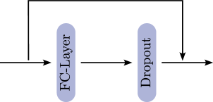
(a) Dropout MLP residual block.

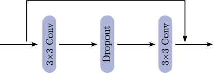
(b) Dropout ResNet residual block.

Figure C.1: Overview of residual blocks.

C.1 (Deep) Ensembles

Deep Ensembles is a popular technique to obtain a BNN (Lakshminarayanan et al., 2017). Each member is a randomly initialized deterministic neural network with the same architecture and parameters are optimized by maximizing the log posterior, i.e., cross-entropy with weight decay. As each optimized member can be seen as a mode of the posterior distribution, we can interpret each ensemble member as a parameter sample of the true posterior distribution.

For Ensembles, we investigate the following hyperparameter in our ablation study:

• Number of ensemble members: 5, 10, 20 (default).
  This hyperparameter describes the number of parameter samples. A high value leads to better approximations of the underlying posterior distribution at the cost of increased computational complexity.

C.2 Dropout

Using Dropout during evaluation leads to a distribution for the predictions corresponding to a variational distribution in the parameter space (Gal et al., 2017). Due to Dropout’s simplicity and efficiency, it is often used for comparison.

For Dropout, we investigate the following hyperparameters in our ablation study:

• Number of ensemble members: 100, 500, 1000 (default)
  This hyperparameter describes the number of parameter samples, i.e., forward passes with Dropout. A high value leads to better approximations of the underlying posterior distribution at the cost of increased computational complexity.

• Dropout rate: 0.25, 0.5 (default), 0.75
  This hyperparameter describes the probability of dropping out a neuron during a forward pass.

C.3 Spectral Normalized Neural Gaussian Process (SNGP)

SNGP (Liu et al., 2020) is a BNN using last-layer LA in combination with spectral normalization (Miyato et al., 2018) and random Fourier features (RFF) (Rahimi & Recht, 2007) to improve the distance-awareness of neural networks. Adding spectral normalization leads to a distance-aware feature space, whereas the composition of RFF and the last-layer LA can be interpreted as an approximate Gaussian process with a Gaussian kernel. A comparison to a typical neural network architecture is depicted in Fig. C.2.

(a) Typical neural network architecture.

(b) SNGP architecture.

Figure C.2: Comparison of typical neural network and SNGP architecture inspired by the visualization of Liu et al. (2022).

For SNGP-MC and SNGP-LA, we investigate the following hyperparameters in our ablation study:

• Number of ensemble members (MC-only): 1000, 10000, 20000 (default)
  This hyperparameter describes the number of parameter samples drawn from the normal distribution obtained via the last-layer LA.

• Number of optimization steps (LA-only): 1 (default), 2, 5
  This hyperparameter describes the number of optimization steps to update the covariance matrix and mean vectors of the normal distribution estimated via LA.

• Norm bound scale (MC and LA): 1.0, 6.0 (default), 12.0
  This hyperparameter describes the upper bound used for spectral normalization of the weight matrices.

• Number of inducing points (MC and LA): 256, 1024 (default), 2048
  This hyperparameter describes the number of random features used for the approximation of the Gaussian kernel.

• Kernel scale (MC and LA): 1.0, 8.0 (default), 256.0
  This hyperparameter describes the width of the Gaussian kernel in the random Fourier feature space.

Appendix D Ablation Study

For an extended discussion of suitable BNN architectures and hyperparameters and as a guide for the usage of Bayesian updates in practice, we present an ablation study in the following. There, we compare the different BNNs regarding their hyperparameters in a one-variable-at-a-time approach. Detailed descriptions of each BNN’s hyperparameters are given in Appendix C.

Table D.1: Ablation study for Ensemble (MC-based updates and inference) as an overview of averaged absolute baseline performances, their relative performance differences to Bayesian updates/retraining, and their computation times. A (${\ast}$) marks a significant performance improvement compared to the respective baseline, and a bold entry indicates the default value for the respective hyperparameter.

Hyper- parameter	Value	ACC $\uparrow$			AUROC $\uparrow$ (entropy)			AUROC $\uparrow$ (variance)			NLL $\downarrow$			TIME [s] $\downarrow$
		base	$\Delta$upd.	$\Delta$retr.	base	$\Delta$upd.	$\Delta$retr.	base	$\Delta$upd.	$\Delta$retr.	base	$\Delta$upd.	$\Delta$retr.	upd.	retr.	pred.
LETTER
Number of ensemble members	5	.539	–.005∗	+.026∗	.675	–.044∗	+.001∗	.754	–.033∗	+.007∗	2.916	+.144∗	–.388∗	.002	29.368	.047
	10	.542	–.004∗	+.028∗	.675	–.041∗	+.003∗	.762	–.046∗	+.009∗	2.928	+.148∗	–.416∗	.004	57.509	.062
	20	.541	–.004∗	+.028∗	.681	–.048∗	+.004∗	.778	–.058∗	+.011∗	2.882	+.141∗	–.406∗	.007	117.945	.107
PENDIGITS
Number of ensemble members	5	.891	+.000∗	+.021∗	.909	–.008∗	+.005∗	.904	–.003∗	+.008∗	.611	+.008∗	–.185∗	.002	29.444	.024
	10	.887	+.000∗	+.019∗	.915	–.007∗	+.004∗	.914	–.005∗	+.007∗	.644	+.003∗	–.183∗	.004	59.344	.035
	20	.892	+.001∗	+.019∗	.916	–.007∗	+.004∗	.915	–.005∗	+.007∗	.559	+.004∗	–.160∗	.007	119.301	.056
MNIST
Number of ensemble members	5	.906	–.004∗	+.021∗	.746	–.047∗	+.012∗	.781	–.020∗	+.007∗	.444	+.037∗	–.172∗	.023	212.947	2.397
	10	.909	–.003∗	+.023∗	.813	–.045∗	+.018∗	.857	–.024∗	+.012∗	.464	+.031∗	–.209∗	.031	418.265	2.603
	20	.908	–.003∗	+.022∗	.843	–.049∗	+.016∗	.891	–.032∗	+.010∗	.439	+.028∗	–.182∗	.048	849.398	3.044
FMNIST
Number of ensemble members	5	.710	–.008∗	+.016∗	.710	–.053∗	–.005∗	.743	–.027∗	–.003∗	1.176	+.114∗	–.185∗	.023	211.435	2.369
	10	.712	–.009∗	+.016∗	.666	–.044∗	–.003∗	.711	–.034∗	–.000∗	1.117	+.125∗	–.160∗	.031	422.343	2.622
	20	.705	–.008∗	+.017∗	.713	–.054∗	–.001∗	.769	–.050∗	+.000∗	1.104	+.109∗	–.164∗	.048	844.109	3.073

Table D.2: Ablation study for Dropout (MC-based updates and inference) as an overview of averaged absolute baseline performances, their relative performance differences to Bayesian updates/retraining, and their computation times. A (${\ast}$) marks a significant performance improvement compared to the respective baseline, and a bold entry indicates the default value for the respective hyperparameter.

Hyper- parameter	Value	ACC $\uparrow$			AUROC $\uparrow$ (entropy)			AUROC $\uparrow$ (variance)			NLL $\downarrow$			TIME [s] $\downarrow$
		base	$\Delta$upd.	$\Delta$retr.	base	$\Delta$upd.	$\Delta$retr.	base	$\Delta$upd.	$\Delta$retr.	base	$\Delta$upd.	$\Delta$retr.	upd.	retr.	pred.
LETTER
Number of ensemble members	100	.537	–.008∗	+.026∗	.629	–.019∗	+.004∗	.679	–.024∗	+.012∗	2.725	+.207∗	–.353∗	.006	5.543	.040
	500	.537	–.007∗	+.026∗	.629	–.016∗	+.004∗	.680	–.018∗	+.012∗	2.719	+.172∗	–.353∗	.003	6.751	.109
	1000	.537	–.006∗	+.026∗	.629	–.014∗	+.004∗	.680	–.019∗	+.012∗	2.718	+.161∗	–.353∗	.006	6.639	.204
Dropout rate	0.25	.535	–.004∗	+.026∗	.622	–.007∗	+.004∗	.658	–.011∗	+.011∗	2.933	+.103∗	–.393∗	.011	6.397	.229
	0.5	.537	–.006∗	+.026∗	.629	–.014∗	+.004∗	.680	–.019∗	+.012∗	2.718	+.161∗	–.353∗	.006	6.639	.204
	0.75	.532	–.002∗	+.026∗	.605	–.001∗	+.000∗	.652	–.003∗	+.009∗	2.532	+.070∗	–.263∗	.012	6.036	.261
PENDIGITS
Number of ensemble members	100	.890	–.001∗	+.021∗	.888	–.003∗	+.006∗	.823	+.003∗	+.011∗	.591	+.021∗	–.179∗	.004	5.249	.019
	500	.890	–.001∗	+.021∗	.889	–.002∗	+.006∗	.823	+.002∗	+.011∗	.590	+.017∗	–.179∗	.003	6.875	.042
	1000	.890	–.000∗	+.021∗	.888	–.001∗	+.006∗	.823	+.002∗	+.011∗	.590	+.012∗	–.179∗	.003	6.631	.064
Dropout rate	0.25	.889	–.000∗	+.021∗	.886	–.000∗	+.006∗	.824	+.001∗	+.010∗	.620	+.006∗	–.188∗	.003	6.553	.064
	0.5	.890	–.000∗	+.021∗	.888	–.001∗	+.006∗	.823	+.002∗	+.011∗	.590	+.012∗	–.179∗	.003	6.631	.064
	0.75	.889	–.000∗	+.020∗	.886	–.001∗	+.006∗	.810	+.002∗	+.011∗	.554	+.018∗	–.149∗	.003	6.685	.065
MNIST
Number of ensemble members	100	.897	–.002∗	+.021∗	.743	–.016∗	+.025∗	.786	–.020∗	+.021∗	.427	+.024∗	–.136∗	.020	40.775	3.318
	500	.897	–.001∗	+.021∗	.745	–.008∗	+.025∗	.792	–.014∗	+.021∗	.426	+.011∗	–.136∗	.039	42.347	7.766
	1000	.897	–.001∗	+.021∗	.745	–.005∗	+.025∗	.793	–.009∗	+.022∗	.426	+.012∗	–.136∗	.060	42.492	13.405
Dropout rate	0.1	.901	–.001∗	+.021∗	.748	–.007∗	+.024∗	.795	–.010∗	+.023∗	.428	+.015∗	–.144∗	.054	42.740	13.358
	0.2	.897	–.001∗	+.021∗	.745	–.005∗	+.025∗	.793	–.009∗	+.022∗	.426	+.012∗	–.136∗	.060	42.492	13.405
	0.5	.867	–.001∗	+.025∗	.714	–.005∗	+.022∗	.795	–.012∗	+.012∗	.496	+.013∗	–.129∗	.061	42.346	13.435
FMNIST
Number of ensemble members	100	.684	–.001∗	+.019∗	.649	–.012∗	+.001∗	.764	–.023∗	+.010∗	1.082	+.022∗	–.150∗	.020	41.548	3.306
	500	.684	–.001∗	+.019∗	.648	–.008∗	+.001∗	.765	–.012∗	+.010∗	1.081	+.024∗	–.150∗	.036	42.818	7.744
	1000	.684	–.001∗	+.019∗	.649	–.005∗	+.001∗	.766	–.012∗	+.010∗	1.081	+.018∗	–.150∗	.058	42.786	13.454
Dropout rate	0.1	.689	–.001∗	+.018∗	.646	–.004∗	+.001∗	.745	–.009∗	+.008∗	1.131	+.021∗	–.158∗	.061	42.548	13.443
	0.2	.684	–.001∗	+.019∗	.649	–.005∗	+.001∗	.766	–.012∗	+.010∗	1.081	+.018∗	–.150∗	.058	42.786	13.454
	0.5	.665	–.001∗	+.019∗	.617	–.001∗	+.001∗	.781	–.007∗	+.012∗	1.041	+.015∗	–.138∗	.056	43.270	13.456

Table D.3: Ablation study for SNGP-MC (MC-based updates and inference) as an overview of averaged absolute baseline performances, their relative performance differences to Bayesian updates/retraining, and their computation times. A (${\ast}$) marks a significant performance improvement compared to the respective baseline, and a bold entry indicates the default value for the respective hyperparameter.

Hyper- parameter	Value	ACC $\uparrow$			AUROC $\uparrow$ (entropy)			AUROC $\uparrow$ (variance)			NLL $\downarrow$			TIME [s] $\downarrow$
		base	$\Delta$upd.	$\Delta$retr.	base	$\Delta$upd.	$\Delta$retr.	base	$\Delta$upd.	$\Delta$retr.	base	$\Delta$upd.	$\Delta$retr.	upd.	retr.	pred.
LETTER
Number of ensemble members	1000	.542	–.023∗	+.029∗	.844	–.029∗	+.015∗	.591	+.013∗	+.016∗	1.909	+.034∗	–.096∗	.019	8.735	.231
	10000	.542	–.009∗	+.029∗	.844	–.013∗	+.015∗	.589	+.025∗	+.016∗	1.909	–.004∗	–.096∗	.056	8.684	2.005
	20000	.542	–.006∗	+.029∗	.844	–.010∗	+.015∗	.589	+.027∗	+.015∗	1.909	–.014∗	–.096∗	.105	8.709	3.895
Norm bound scale	0.5	.542	–.002∗	+.029∗	.843	–.006∗	+.016∗	.609	+.015∗	+.015∗	1.899	–.025∗	–.096∗	.104	8.446	3.784
	1.0	.542	–.006∗	+.029∗	.844	–.010∗	+.015∗	.589	+.027∗	+.015∗	1.909	–.014∗	–.096∗	.105	8.709	3.895
	2.0	.540	–.007∗	+.029∗	.841	–.011∗	+.015∗	.588	+.030∗	+.016∗	1.914	–.013∗	–.096∗	.104	8.457	3.638
Number of inducing points	256	.535	–.010∗	+.029∗	.844	–.012∗	+.016∗	.501	+.056∗	+.012∗	1.953	–.004∗	–.094∗	.083	8.385	3.987
	1024	.542	–.006∗	+.029∗	.844	–.010∗	+.015∗	.589	+.027∗	+.015∗	1.909	–.014∗	–.096∗	.105	8.709	3.895
	2048	.552	–.006∗	+.029∗	.838	–.007∗	+.014∗	.601	+.021∗	+.017∗	1.881	–.019∗	–.096∗	.168	8.996	4.053
Kernel scale	1.0	.246	–.099∗	+.017∗	.627	–.072∗	+.010∗	.463	+.031∗	–.004∗	3.017	+.105∗	–.024∗	.105	8.821	4.054
	8.0	.542	–.006∗	+.029∗	.844	–.010∗	+.015∗	.589	+.027∗	+.015∗	1.909	–.014∗	–.096∗	.105	8.709	3.895
	256.0	.491	+.010∗	+.030∗	.738	+.010∗	+.020∗	.576	+.022∗	+.020∗	1.994	–.051∗	–.117∗	.101	8.881	4.051
PENDIGITS
Number of ensemble members	1000	.890	+.003∗	+.021∗	.941	–.003∗	+.008∗	.920	–.014∗	+.012∗	.505	–.039∗	–.071∗	.012	8.853	.037
	10000	.890	+.007∗	+.021∗	.941	+.001∗	+.008∗	.920	–.005∗	+.012∗	.506	–.048∗	–.072∗	.029	8.784	.453
	20000	.890	+.008∗	+.021∗	.941	+.002∗	+.008∗	.920	+.001∗	+.012∗	.505	–.049∗	–.071∗	.049	8.611	.884
Norm bound scale	0.5	.887	+.008∗	+.021∗	.937	+.003∗	+.008∗	.910	+.002∗	+.011∗	.514	–.047∗	–.071∗	.047	8.952	.871
	1.0	.890	+.008∗	+.021∗	.941	+.002∗	+.008∗	.920	+.001∗	+.012∗	.505	–.049∗	–.071∗	.049	8.611	.884
	2.0	.890	+.008∗	+.021∗	.941	+.003∗	+.008∗	.920	+.002∗	+.012∗	.505	–.049∗	–.072∗	.047	8.759	.863
Number of inducing points	256	.895	+.008∗	+.020∗	.954	+.000∗	+.008∗	.924	+.004∗	+.014∗	.487	–.048∗	–.069∗	.031	8.211	.870
	1024	.890	+.008∗	+.021∗	.941	+.002∗	+.008∗	.920	+.001∗	+.012∗	.505	–.049∗	–.071∗	.049	8.611	.884
	2048	.897	+.009∗	+.021∗	.943	+.003∗	+.010∗	.926	–.005∗	+.011∗	.491	–.049∗	–.072∗	.075	8.829	.864
Kernel scale	1.0	.800	–.035∗	+.032∗	.886	–.023∗	+.018∗	.769	–.013∗	+.021∗	1.042	–.025∗	–.088∗	.047	8.883	.873
	8.0	.890	+.008∗	+.021∗	.941	+.002∗	+.008∗	.920	+.001∗	+.012∗	.505	–.049∗	–.071∗	.049	8.611	.884
	256.0	.862	+.011∗	+.029∗	.888	+.011∗	+.016∗	.806	+.025∗	+.024∗	.575	–.049∗	–.093∗	.042	8.775	.844
MNIST
Number of ensemble members	1000	.886	+.002∗	+.025∗	.920	–.001∗	+.006∗	.890	–.004∗	+.009∗	.424	–.022∗	–.087∗	.029	46.322	2.340
	10000	.886	+.005∗	+.025∗	.919	–.001∗	+.005∗	.890	+.007∗	+.009∗	.425	–.030∗	–.087∗	.049	46.046	3.715
	20000	.886	+.005∗	+.025∗	.920	+.000∗	+.005∗	.890	+.002∗	+.008∗	.424	–.029∗	–.087∗	.064	46.885	5.219
Norm bound scale	1.0	.887	+.005∗	+.025∗	.923	+.001∗	+.005∗	.894	+.005∗	+.008∗	.424	–.031∗	–.088∗	.064	46.287	5.226
	6.0	.886	+.005∗	+.025∗	.920	+.000∗	+.005∗	.890	+.002∗	+.008∗	.424	–.029∗	–.087∗	.064	46.885	5.219
	12.0	.886	+.005∗	+.025∗	.919	+.000∗	+.005∗	.889	+.002∗	+.009∗	.424	–.030∗	–.087∗	.058	47.607	5.157
Number of inducing points	256	.891	+.004∗	+.024∗	.919	–.000∗	+.009∗	.895	+.003∗	+.011∗	.408	–.028∗	–.084∗	.054	46.628	5.239
	1024	.886	+.005∗	+.025∗	.920	+.000∗	+.005∗	.890	+.002∗	+.008∗	.424	–.029∗	–.087∗	.064	46.885	5.219
	2048	.885	+.005∗	+.025∗	.910	–.000∗	+.009∗	.887	+.006∗	+.010∗	.430	–.028∗	–.088∗	.096	47.102	5.338
Kernel scale	1.0	.886	+.005∗	+.025∗	.920	+.000∗	+.005∗	.890	+.002∗	+.008∗	.424	–.029∗	–.087∗	.064	46.885	5.219
	8.0	.883	+.005∗	+.027∗	.909	+.003∗	+.009∗	.894	+.006∗	+.007∗	.435	–.032∗	–.095∗	.058	47.591	5.222
	256.0	.810	+.006∗	+.036∗	.842	+.001∗	+.020∗	.845	+.007∗	+.011∗	.641	–.032∗	–.119∗	.065	46.441	5.210
FMNIST
Number of ensemble members	1000	.685	+.002∗	+.018∗	.764	–.009∗	–.001∗	.709	–.027∗	–.001∗	.922	–.016∗	–.067∗	.028	46.862	2.281
	10000	.685	+.004∗	+.018∗	.764	–.013∗	–.001∗	.709	–.013∗	–.001∗	.922	–.024∗	–.067∗	.048	46.718	3.733
	20000	.685	+.005∗	+.018∗	.764	–.009∗	–.001∗	.709	–.010∗	–.001∗	.922	–.030∗	–.067∗	.058	46.536	5.083
Norm bound scale	1.0	.685	+.005∗	+.019∗	.771	–.010∗	–.001∗	.715	–.009∗	–.001∗	.923	–.030∗	–.067∗	.060	46.920	5.169
	6.0	.685	+.005∗	+.018∗	.764	–.009∗	–.001∗	.709	–.010∗	–.001∗	.922	–.030∗	–.067∗	.058	46.536	5.083
	12.0	.685	+.005∗	+.018∗	.764	–.009∗	–.001∗	.709	–.010∗	–.001∗	.922	–.030∗	–.067∗	.065	47.333	5.135
Number of inducing points	256	.684	+.006∗	+.019∗	.742	–.005∗	+.006∗	.688	+.002∗	+.005∗	.941	–.030∗	–.065∗	.047	47.339	5.138
	1024	.685	+.005∗	+.018∗	.764	–.009∗	–.001∗	.709	–.010∗	–.001∗	.922	–.030∗	–.067∗	.058	46.536	5.083
	2048	.689	+.005∗	+.018∗	.756	–.007∗	–.004∗	.699	–.003∗	–.004∗	.918	–.027∗	–.063∗	.091	47.148	5.194
Kernel scale	1.0	.685	+.005∗	+.018∗	.764	–.009∗	–.001∗	.709	–.010∗	–.001∗	.922	–.030∗	–.067∗	.058	46.536	5.083
	8.0	.686	+.005∗	+.018∗	.740	–.014∗	–.001∗	.684	–.004∗	–.001∗	.925	–.035∗	–.073∗	.059	46.468	5.078
	256.0	.651	+.006∗	+.024∗	.683	–.002∗	–.003∗	.519	+.022∗	+.013∗	.981	–.031∗	–.088∗	.063	47.568	5.109

Table D.4: Ablation study for SNGP-LA (LA-based updates and inference via mean-field approximation) as an overview of averaged absolute baseline performances, their relative performance differences to Bayesian updates/retraining, and their computation times. A (${\ast}$) marks a significant performance improvement compared to the respective baseline, and a bold entry indicates the default value for the respective hyperparameter.

Hyper- parameter	Value	ACC $\uparrow$			AUROC $\uparrow$ (entropy)			AUROC $\uparrow$ (variance)			NLL $\downarrow$			TIME [s] $\downarrow$
		base	$\Delta$upd.	$\Delta$retr.	base	$\Delta$upd.	$\Delta$retr.	base	$\Delta$upd.	$\Delta$retr.	base	$\Delta$upd.	$\Delta$retr.	upd.	retr.	pred.
LETTER
Number of optimization steps	1	.543	+.015∗	+.029∗	.845	+.007∗	+.015∗	.833	+.002∗	+.015∗	1.929	–.051∗	–.095∗	.141	8.727	.040
	2	.543	+.026∗	+.029∗	.845	+.013∗	+.015∗	.833	+.003∗	+.015∗	1.929	–.085∗	–.095∗	.293	9.070	.041
	5	.543	+.037∗	+.029∗	.845	+.022∗	+.015∗	.833	+.006∗	+.015∗	1.929	–.136∗	–.095∗	.699	8.679	.040
Norm bound scale	0.5	.542	+.015∗	+.029∗	.844	+.007∗	+.016∗	.827	+.002∗	+.015∗	1.917	–.052∗	–.095∗	.146	8.445	.040
	1.0	.543	+.015∗	+.029∗	.845	+.007∗	+.015∗	.833	+.002∗	+.015∗	1.929	–.051∗	–.095∗	.141	8.727	.040
	2.0	.540	+.015∗	+.029∗	.841	+.007∗	+.015∗	.832	+.002∗	+.015∗	1.933	–.051∗	–.095∗	.147	8.801	.041
Number of inducing points	256	.535	+.013∗	+.029∗	.843	+.006∗	+.016∗	.816	+.002∗	+.015∗	1.973	–.046∗	–.093∗	.017	8.032	.039
	1024	.543	+.015∗	+.029∗	.845	+.007∗	+.015∗	.833	+.002∗	+.015∗	1.929	–.051∗	–.095∗	.141	8.727	.040
	2048	.552	+.016∗	+.028∗	.838	+.007∗	+.014∗	.821	+.002∗	+.014∗	1.900	–.052∗	–.095∗	.877	8.939	.039
Kernel scale	1.0	.247	+.013∗	+.017∗	.628	+.006∗	+.010∗	.570	+.000∗	+.007∗	3.032	–.013∗	–.023∗	.147	8.908	.041
	8.0	.543	+.015∗	+.029∗	.845	+.007∗	+.015∗	.833	+.002∗	+.015∗	1.929	–.051∗	–.095∗	.141	8.727	.040
	256.0	.491	+.014∗	+.030∗	.740	+.011∗	+.020∗	.661	+.002∗	+.022∗	1.999	–.054∗	–.114∗	.146	8.728	.040
PENDIGITS
Number of optimization steps	1	.890	+.013∗	+.021∗	.941	+.007∗	+.008∗	.940	+.004∗	+.009∗	.502	–.045∗	–.072∗	.144	8.724	.023
	2	.890	+.020∗	+.021∗	.941	+.010∗	+.008∗	.940	+.007∗	+.009∗	.502	–.069∗	–.072∗	.269	8.619	.023
	5	.890	+.025∗	+.021∗	.941	+.012∗	+.008∗	.940	+.011∗	+.009∗	.502	–.101∗	–.072∗	.688	8.826	.023
Norm bound scale	0.5	.887	+.013∗	+.021∗	.937	+.007∗	+.008∗	.933	+.005∗	+.009∗	.511	–.045∗	–.071∗	.146	8.519	.023
	1.0	.890	+.013∗	+.021∗	.941	+.007∗	+.008∗	.940	+.004∗	+.009∗	.502	–.045∗	–.072∗	.144	8.724	.023
	2.0	.890	+.013∗	+.021∗	.941	+.007∗	+.008∗	.940	+.004∗	+.009∗	.501	–.045∗	–.072∗	.145	8.700	.022
Number of inducing points	256	.895	+.014∗	+.020∗	.954	+.006∗	+.008∗	.949	+.005∗	+.010∗	.484	–.044∗	–.069∗	.017	8.171	.022
	1024	.890	+.013∗	+.021∗	.941	+.007∗	+.008∗	.940	+.004∗	+.009∗	.502	–.045∗	–.072∗	.144	8.724	.023
	2048	.898	+.015∗	+.021∗	.942	+.008∗	+.010∗	.944	+.004∗	+.010∗	.488	–.047∗	–.072∗	.737	9.173	.022
Kernel scale	1.0	.801	+.025∗	+.032∗	.886	+.012∗	+.018∗	.841	+.006∗	+.021∗	1.043	–.045∗	–.089∗	.148	8.903	.023
	8.0	.890	+.013∗	+.021∗	.941	+.007∗	+.008∗	.940	+.004∗	+.009∗	.502	–.045∗	–.072∗	.144	8.724	.023
	256.0	.862	+.012∗	+.029∗	.887	+.014∗	+.016∗	.843	+.010∗	+.026∗	.570	–.044∗	–.093∗	.138	8.833	.023
MNIST
Number of optimization steps	1	.886	+.006∗	+.025∗	.920	+.003∗	+.006∗	.936	+.003∗	+.005∗	.423	–.028∗	–.086∗	.168	46.247	2.229
	2	.886	+.009∗	+.025∗	.922	+.003∗	+.006∗	.937	+.004∗	+.005∗	.423	–.040∗	–.086∗	.305	46.527	2.286
	5	.886	+.011∗	+.025∗	.923	+.001∗	+.005∗	.937	+.003∗	+.005∗	.423	–.053∗	–.086∗	.716	46.615	2.268
Norm bound scale	1.0	.886	+.007∗	+.025∗	.921	+.003∗	+.005∗	.934	+.003∗	+.004∗	.423	–.029∗	–.087∗	.169	46.243	2.243
	6.0	.886	+.006∗	+.025∗	.920	+.003∗	+.006∗	.936	+.003∗	+.005∗	.423	–.028∗	–.086∗	.168	46.247	2.229
	12.0	.886	+.006∗	+.025∗	.922	+.003∗	+.005∗	.936	+.003∗	+.005∗	.422	–.029∗	–.086∗	.166	45.674	2.242
Number of inducing points	256	.889	+.006∗	+.025∗	.920	+.002∗	+.008∗	.930	+.002∗	+.008∗	.410	–.028∗	–.084∗	.040	47.838	2.291
	1024	.886	+.006∗	+.025∗	.920	+.003∗	+.006∗	.936	+.003∗	+.005∗	.423	–.028∗	–.086∗	.168	46.247	2.229
	2048	.885	+.006∗	+.026∗	.909	+.003∗	+.009∗	.922	+.005∗	+.007∗	.427	–.027∗	–.087∗	.783	46.486	2.262
Kernel scale	1.0	.886	+.006∗	+.025∗	.920	+.003∗	+.006∗	.936	+.003∗	+.005∗	.423	–.028∗	–.086∗	.168	46.247	2.229
	8.0	.883	+.006∗	+.027∗	.908	+.004∗	+.008∗	.922	+.005∗	+.006∗	.434	–.030∗	–.093∗	.158	46.756	2.289
	256.0	.809	+.007∗	+.036∗	.845	+.002∗	+.018∗	.882	+.004∗	+.012∗	.639	–.029∗	–.118∗	.169	46.819	2.263
FMNIST
Number of optimization steps	1	.685	+.006∗	+.018∗	.764	–.005∗	+.001∗	.863	–.000∗	+.006∗	.924	–.034∗	–.066∗	.166	46.308	2.251
	2	.685	+.008∗	+.018∗	.763	–.010∗	+.000∗	.862	–.002∗	+.006∗	.925	–.045∗	–.066∗	.304	45.951	2.260
	5	.685	+.007∗	+.018∗	.764	–.020∗	–.001∗	.862	–.009∗	+.005∗	.925	–.045∗	–.066∗	.709	46.525	2.274
Norm bound scale	1.0	.685	+.006∗	+.018∗	.758	–.004∗	–.001∗	.859	+.000∗	+.004∗	.928	–.035∗	–.066∗	.168	46.380	2.269
	6.0	.685	+.006∗	+.018∗	.764	–.005∗	+.001∗	.863	–.000∗	+.006∗	.924	–.034∗	–.066∗	.166	46.308	2.251
	12.0	.685	+.006∗	+.018∗	.764	–.005∗	–.001∗	.861	–.001∗	+.006∗	.924	–.035∗	–.066∗	.168	45.763	2.246
Number of inducing points	256	.683	+.007∗	+.019∗	.743	–.000∗	+.004∗	.835	+.001∗	+.011∗	.944	–.036∗	–.065∗	.040	46.016	2.265
	1024	.685	+.006∗	+.018∗	.764	–.005∗	+.001∗	.863	–.000∗	+.006∗	.924	–.034∗	–.066∗	.166	46.308	2.251
	2048	.689	+.006∗	+.017∗	.751	–.002∗	–.002∗	.849	+.000∗	+.005∗	.920	–.031∗	–.062∗	1.045	45.600	2.252
Kernel scale	1.0	.685	+.006∗	+.018∗	.764	–.005∗	+.001∗	.863	–.000∗	+.006∗	.924	–.034∗	–.066∗	.166	46.308	2.251
	8.0	.686	+.006∗	+.018∗	.730	–.009∗	–.001∗	.844	–.001∗	+.005∗	.927	–.039∗	–.072∗	.169	45.481	2.240
	256.0	.650	+.007∗	+.024∗	.683	–.003∗	–.001∗	.774	+.000∗	+.022∗	.980	–.030∗	–.087∗	.170	46.289	2.277

Appendix E Performance Curves

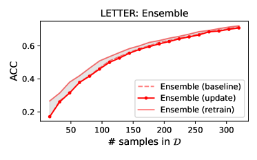
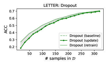
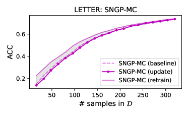
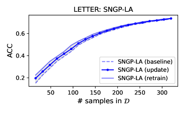
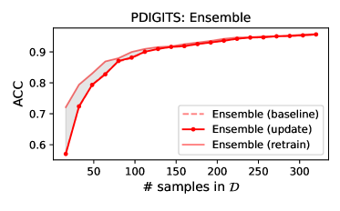
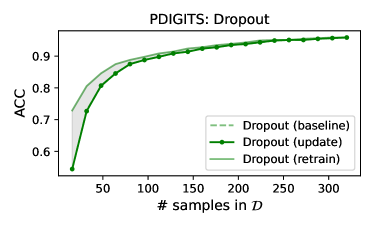
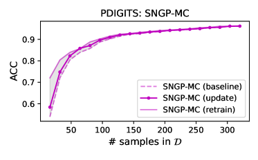
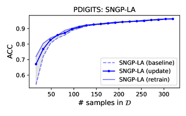
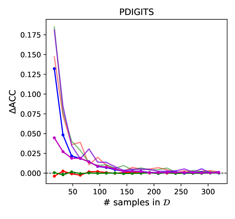
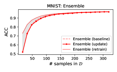
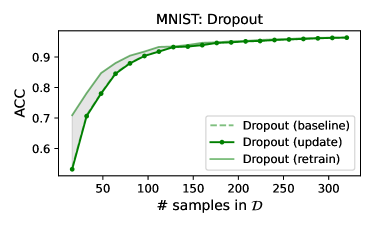
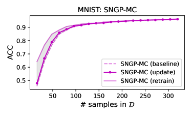
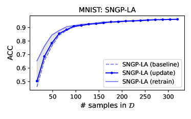
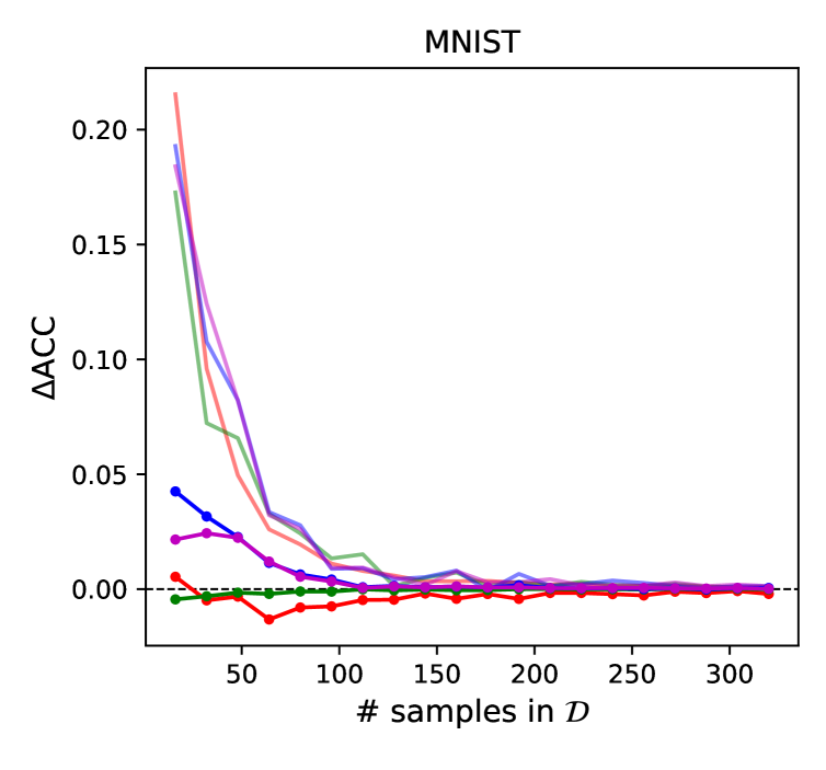
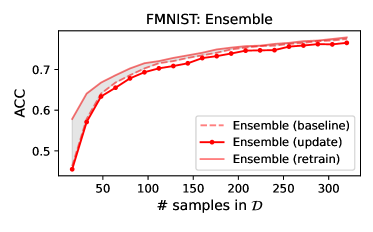
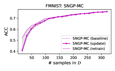
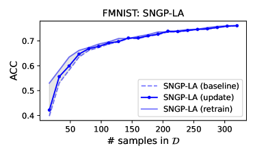
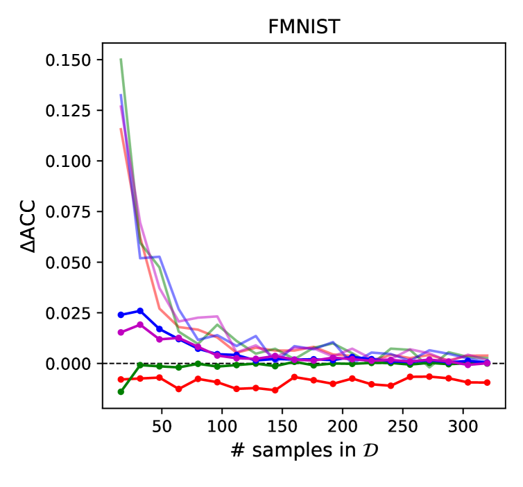
Figure E.1: ACC curves of four BNNs for four datasets showing absolute ACC (left, center column) and ACC differences (right column) between the baseline BNN and the retrained respectively Bayesian updated BNN.

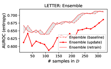
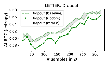
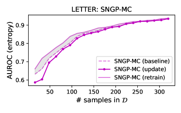
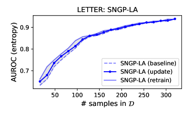
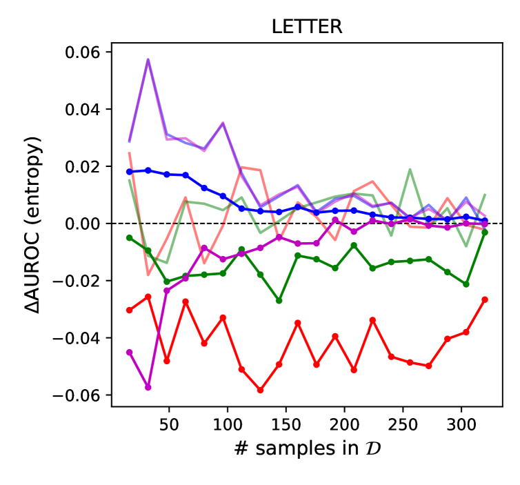
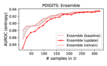
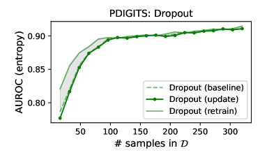
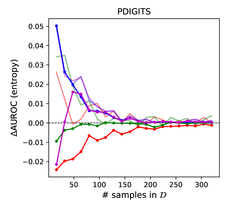
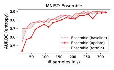
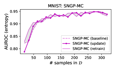
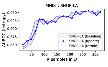
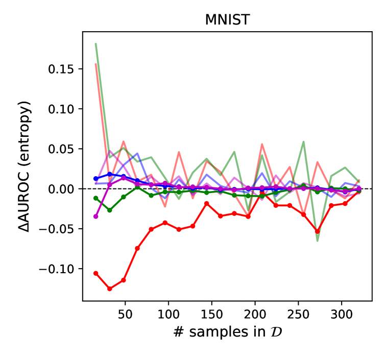
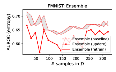
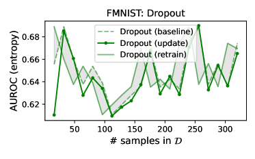
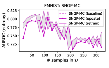
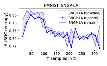
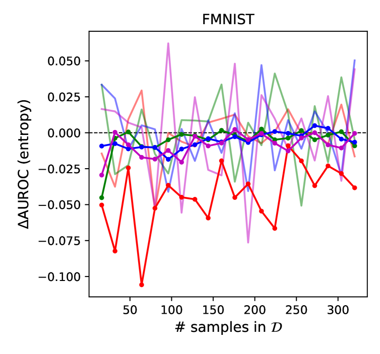
Figure E.2: AUROC (entropy) curves of four BNNs for four datasets showing absolute AUROC (left, center column) and AUROC differences (right column) between the baseline BNN and the retrained respectively Bayesian updated BNN.

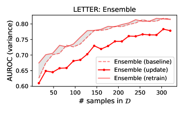
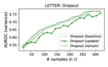
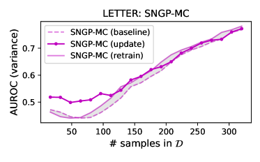
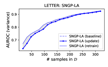
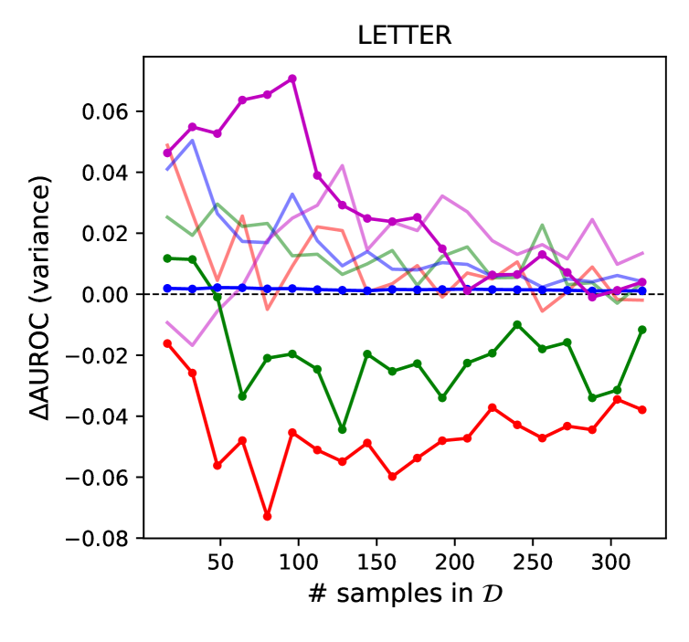
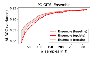
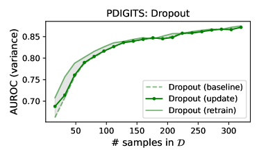
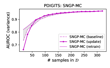
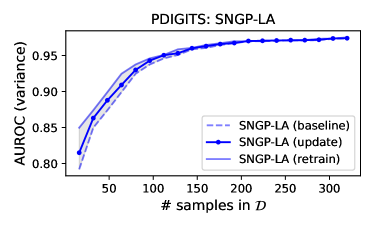
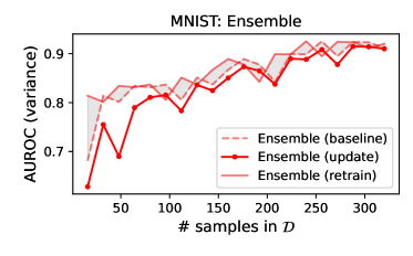
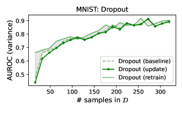
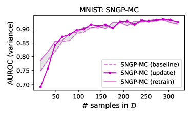
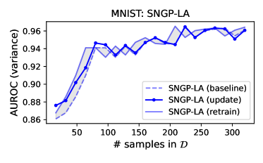
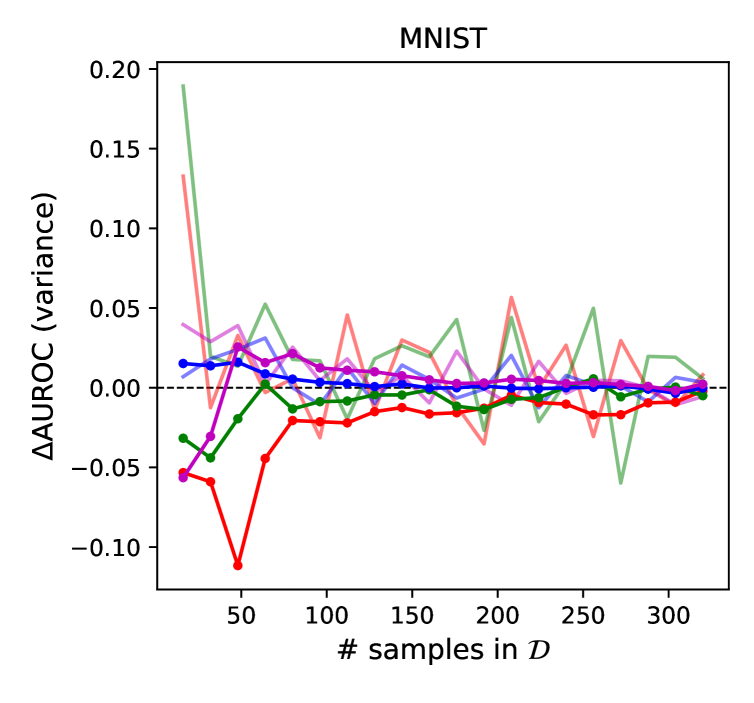
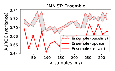
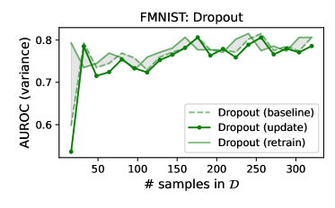
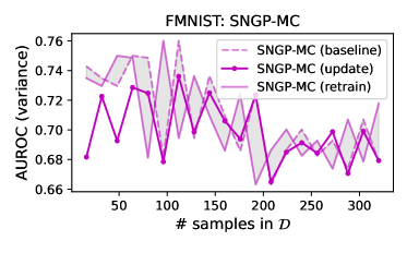
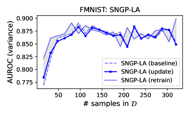
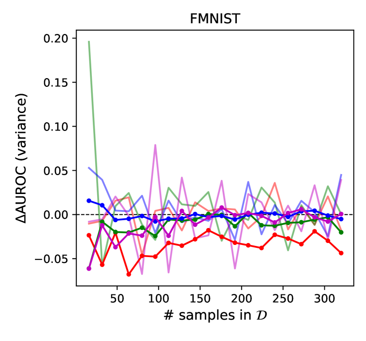
Figure E.3: AUROC (variance) curves of four BNNs for four datasets showing absolute AUROC (left, center column) and AUROC differences (right column) between the baseline BNN and the retrained respectively Bayesian updated BNN.

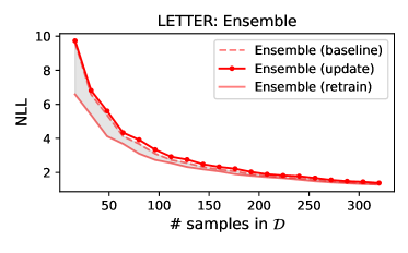
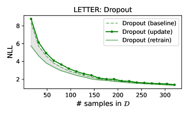
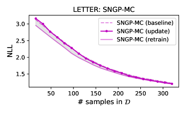
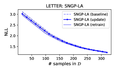
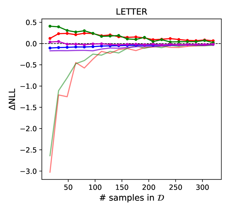
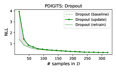
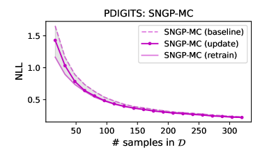
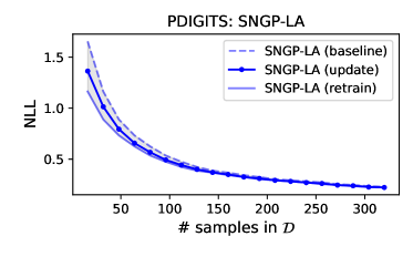
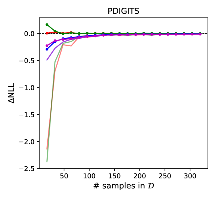
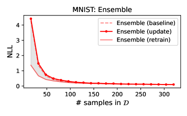
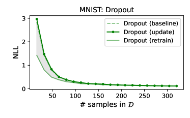
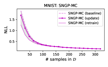
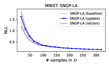
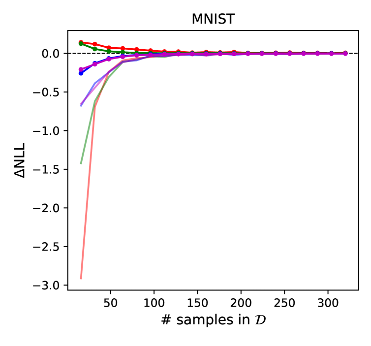
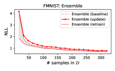
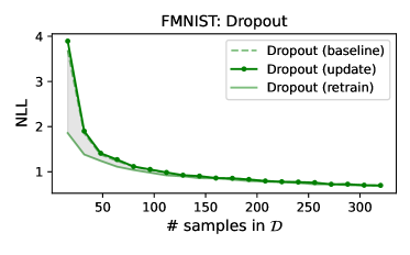
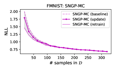
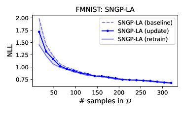
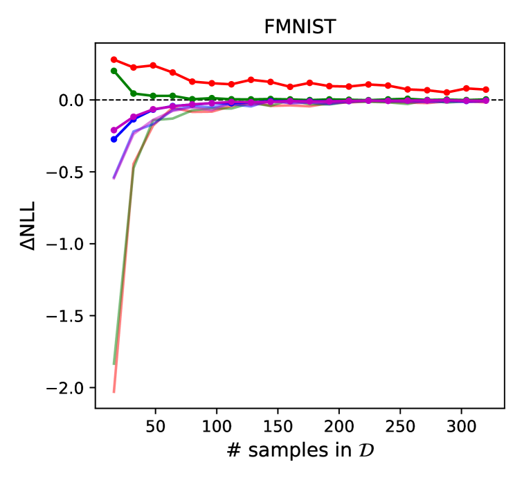
Figure E.4: NLL curves of four BNNs for four datasets showing absolute NLL (left, center column) and NLL differences (right column) between the baseline BNN and the retrained respectively Bayesian updated BNN.

Appendix F Details about the active learning use case

In this appendix, we will describe the experimental setup for our active learning use case and complement Section 5 by accuracy (i.e., learning) curves.

We start the active learning process with 16 labeled samples which are randomly selected. In each active learning cycle, a subset of 1000 data samples is randomly selected as label candidates from the unlabeled dataset. The top-$b$ strategies (and BatchBALD) select the top 32 most valuable candidates at one time. In contrast, the Bayesian update variants of these strategies will select only one sample from the candidates for labeling and then perform LA-based Bayesian updates for each. In this case, the updating process will be executed 31 times ($b$ = 31). In any case, a retraining is performed after an active learning cycle in which 32 labels are obtained. We perform 15 active learning cycles on the datasets PDIGITS, 30 on MNIST and FMNIST, and 50 on LETTER, respectively. We also repeat each experiment 10 times.

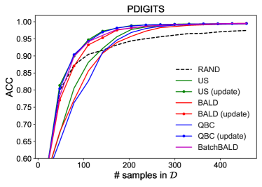
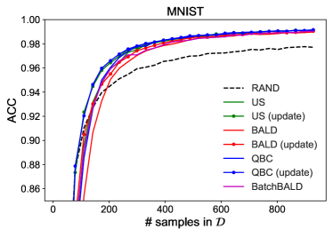
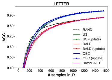
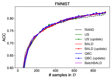
Figure F.1: Accuracy curves for the four benchmark datasets. The results are averaged over 10 repetitions. All query strategies using Bayesian updates perform superior to their respective top-$b$ counterpart by reaching a higher accuracy with less labeled samples.

As a result, we present learning curves in Figure F.1, which show the accuracy with respect to the number of acquired labels. The accuracy curves on the FMNIST dataset can not show the apparent differences between query strategies in the figure, and for detail, please check Table 3. We mainly discuss the accuracy curves of the other three benchmark datasets in the following. During the early active learning phase, the top-$b$ strategies likely select uninformative instances and perform poorly, and even random sampling performs better. However, Bayesian update strategies likely select more diverse samples and surpass random sampling much earlier than top-$b$. BatchBALD and Bayesian updated BALD perform similarly well and their performance difference is never significant. The combination of Bayesian updates with US and QBC yields similar performance, and both perform better than BatchBALD on different datasets (except FMNIST but the differences are not significant). The performance of BatchBALD depends on the dataset. For example, on the LETTER dataset, the area under the accuracy curve of BatchBALD is even lower than random sampling. In contrast, the conventional active learning strategies such as US and QBC with Bayesian updates show consistently high performance on different datasets, especially in the early stage of active learning.

We suppose that our proposed method SNGP with LA-based Bayesian updates addresses two problems in applying deep active learning: (i) our idea selects more diverse samples than the top-$b$ approach; (ii) Bayesian updates will significantly reduce the cost of retraining, which is shown in Table 2. Moreover, the performance of our method is comparable to or even higher than BatchBALD on different data sets. This method can also be applied to some strategies unsuitable for active deep learning, such as expected error reduction (Roy & McCallum, 2001) and probabilistic active learning (Kottke et al., 2021), which require retraining the model for each selection candidate. Nevertheless, Bayesian updates limit the possible model choices to those that are appropriate such as SNGP.

References

- Beluch et al. (2018) William H. Beluch, Tim Genewein, Andreas Nürnberger, and Jan M. Köhler. The power of ensembles for active learning in image classification. In IEEE Conference on Computer Vision and Pattern Recognition, pp. 9368–9377, 2018.
- Bishop (2006) Christopher M Bishop. Pattern recognition and machine learning. Springer, 2006.
- Daxberger et al. (2021) Erik Daxberger, Agustinus Kristiadi, Alexander Immer, Runa Eschenhagen, Matthias Bauer, and Philipp Hennig. Laplace redux-effortless Bayesian deep learning. Advances in Neural Information Processing Systems, 2021.
- De Lange et al. (2021) Matthias De Lange, Rahaf Aljundi, Marc Masana, Sarah Parisot, Xu Jia, Aleš Leonardis, Gregory Slabaugh, and Tinne Tuytelaars. A continual learning survey: Defying forgetting in classification tasks. IEEE Transactions on Pattern Analysis and Machine Intelligence, 44(7):3366–3385, 2021.
- Dua & Graff (2017) Dheeru Dua and Casey Graff. UCI Machine Learning Repository, 2017.
- Eschenhagen et al. (2021) Runa Eschenhagen, Erik Daxberger, Philipp Hennig, and Agustinus Kristiadi. Mixtures of Laplace approximations for improved post-hoc uncertainty in deep learning. In Bayesian Deep Learning Workshop at NeurIPS, 2021.
- Fortuin (2022) Vincent Fortuin. Priors in Bayesian deep learning: A review. International Statistical Review, 2022.
- Frey & Slate (1991) Peter W Frey and David J Slate. Letter recognition using holland-style adaptive classifiers. Machine Learning, 6(2):161–182, 1991.
- Gal & Ghahramani (2016) Yarin Gal and Zoubin Ghahramani. Dropout as a Bayesian approximation: Representing model uncertainty in deep learning. In International Conference on Machine Learning, pp. 1050–1059, 2016.
- Gal et al. (2017) Yarin Gal, Riashat Islam, and Zoubin Ghahramani. Deep Bayesian active learning with image data. In International Conference on Machine Learning, pp. 1183–1192, 2017.
- Guo et al. (2017) Chuan Guo, Geoff Pleiss, Yu Sun, and Kilian Q Weinberger. On calibration of modern neural networks. In International Conference on Machine Learning, pp. 1321–1330, 2017.
- He et al. (2016) Kaiming He, Xiangyu Zhang, Shaoqing Ren, and Jian Sun. Deep residual learning for image recognition. In IEEE Conference on Computer Vision and Pattern Recognition, pp. 770–778, 2016.
- Hobbhahn et al. (2022) Marius Hobbhahn, Agustinus Kristiadi, and Philipp Hennig. Fast predictive uncertainty for classification with Bayesian deep networks. In Uncertainty in Artificial Intelligence, pp. 822–832, 2022.
- Hoi et al. (2021) Steven C H Hoi, Doyen Sahoo, Jing Lu, and Peilin Zhao. Online learning: A comprehensive survey. Neurocomputing, 459:249–289, 2021.
- Jospin et al. (2022) Laurent Valentin Jospin, Hamid Laga, Farid Boussaid, Wray Buntine, and Mohammed Bennamoun. Hands-on Bayesian neural networks – A tutorial for deep learning users. IEEE Computational Intelligence Magazine, 17(2):29–48, 2022.
- Kirkpatrick et al. (2017) James Kirkpatrick, Razvan Pascanu, Neil Rabinowitz, Joel Veness, Guillaume Desjardins, Andrei A Rusu, Kieran Milan, John Quan, Tiago Ramalho, Agnieszka Grabska-Barwinska, Demis Hassabis, Claudia Clopath, Dharshan Kumaran, and Raia Hadsell. Overcoming catastrophic forgetting in neural networks. Proceedings of the National Academy of Sciences, 114(13):3521–3526, 2017.
- Kirsch et al. (2019) Andreas Kirsch, Joost Van Amersfoort, and Yarin Gal. BatchBALD: Efficient and diverse batch acquisition for deep Bayesian active learning. In Advances in Neural Information Processing Systems, 2019.
- Kirsch et al. (2022) Andreas Kirsch, Jannik Kossen, and Yarin Gal. Marginal and Joint Cross-Entropies & Predictives for Online Bayesian Inference, Active Learning, and Active Sampling. arXiv preprint arXiv:2205.08766, 2022.
- Kottke et al. (2021) Daniel Kottke, Marek Herde, Christoph Sandrock, Denis Huseljic, Georg Krempl, and Bernhard Sick. Toward optimal probabilistic active learning using a Bayesian approach. Machine Learning, 110(6):1199–1231, 2021.
- Krizhevsky (2009) Alex Krizhevsky. Learning multiple layers of features from tiny images. Master’s thesis, University of Toronto, 2009.
- Lakshminarayanan et al. (2017) Balaji Lakshminarayanan, Alexander Pritzel, and Charles Blundell. Simple and scalable predictive uncertainty estimation using deep ensembles. In Advances in Neural Information Processing Systems, 2017.
- LeCun & Cortes (1998) Yann LeCun and Corinna Cortes. The MNIST database of handwritten digits, 1998.
- Lewis & Catlett (1994) David D Lewis and Jason Catlett. Heterogeneous uncertainty sampling for supervised learning. In Machine Learning Proceedings, pp. 148–156, 1994.
- Liu et al. (2020) Jeremiah Liu, Zi Lin, Shreyas Padhy, Dustin Tran, Tania Bedrax Weiss, and Balaji Lakshminarayanan. Simple and principled uncertainty estimation with deterministic deep learning via distance awareness. In Advances in Neural Information Processing Systems, 2020.
- Liu et al. (2022) Jeremiah Zhe Liu, Shreyas Padhy, Jie Ren, Zi Lin, Yeming Wen, Ghassen Jerfel, Zack Nado, Jasper Snoek, Dustin Tran, and Balaji Lakshminarayanan. A Simple Approach to Improve Single-Model Deep Uncertainty via Distance-Awareness. arXiv preprint arXiv:2205.00403, 2022.
- Loshchilov & Hutter (2017) Ilya Loshchilov and Frank Hutter. SGDR: Stochastic gradient descent with warm restarts. In International Conference on Learning Representations, 2017.
- Lu et al. (2020) Zhiyun Lu, Eugene Ie, and Fei Sha. Mean-field approximation to Gaussian-softmax integral with application to uncertainty estimation. arXiv preprint arXiv:2006.07584, 2020.
- Miyato et al. (2018) Takeru Miyato, Toshiki Kataoka, Masanori Koyama, and Yuichi Yoshida. Spectral normalization for generative adversarial networks. In International Conference on Learning Representations, 2018.
- Opper & Winther (1999) Manfred Opper and Ole Winther. A Bayesian approach to on-line learning. In On-line Learning in Neural Networks, Publications of the Newton Institute, pp. 363–378, 1999.
- Ovadia et al. (2019) Yaniv Ovadia, Emily Fertig, Jie Ren, Zachary Nado, David Sculley, Sebastian Nowozin, Joshua Dillon, Balaji Lakshminarayanan, and Jasper Snoek. Can you trust your model’s uncertainty? Evaluating predictive uncertainty under dataset shift. Advances in Neural Information Processing Systems, 2019.
- Rahimi & Recht (2007) Ali Rahimi and Benjamin Recht. Random features for large-scale kernel machines. In Advances in Neural Information Processing Systems, 2007.
- Ren et al. (2021) Pengzhen Ren, Yun Xiao, Xiaojun Chang, Po-Yao Huang, Zhihui Li, Brij B. Gupta, Xiaojiang Chen, and Xin Wang. A survey of deep active learning. ACM Computing Surveys, 54(9):1–40, 2021.
- Ritter et al. (2018a) Hippolyt Ritter, Aleksandar Botev, and David Barber. Online structured Laplace approximations for overcoming catastrophic forgetting. In Advances in Neural Information Processing Systems, 2018a.
- Ritter et al. (2018b) Hippolyt Ritter, Aleksandar Botev, and David Barber. A scalable Laplace approximation for neural networks. In International Conference on Learning Representations, 2018b.
- Roy & McCallum (2001) Nicholas Roy and Andrew McCallum. Toward optimal active learning through sampling estimation of error reduction. In International Conference on Machine Learning, 2001.
- Sahoo et al. (2018) Doyen Sahoo, Quang Pham, Jing Lu, and Steven CH Hoi. Online deep learning: learning deep neural networks on the fly. In International Joint Conference on Artificial Intelligence, pp. 2660–2666, 2018.
- Sener & Savarese (2018) Ozan Sener and Silvio Savarese. Active learning for convolutional neural networks: A core-set approach. In International Conference on Learning Representations, 2018.
- Settles (2009) Burr Settles. Active learning literature survey. Computer Sciences Technical Report 1648, University of Wisconsin–Madison, 2009.
- Seung et al. (1992) Hyunjune S Seung, Manfred Opper, and Haim Sompolinsky. Query by committee. In Workshop on Computational Learning Theory, pp. 287–294, 1992.