Vulnerabilities of Single-Round Incentive Compatibility in Auto-bidding: Theory and Evidence from ROI-Constrained Online Advertising Markets

Abstract

Most of the work in auction design literature assumes that bidders behave rationally based on the information available for every individual auction, and the revelation principle enables designers to restrict their efforts to incentive compatible (IC) mechanisms. However, in today’s online advertising markets, one of the most important real-life applications of auction design, the data and computational power required to bid optimally are only available to the auction designer, and an advertiser can only participate by setting performance objectives and constraints for its proxy auto-bidder provided by the platform.

The prevalence of auto-bidding necessitates a review of auction theory. In this paper, we examine properties of auto-bidding markets through the lens of ROI-constrained value-maximizing campaigns, which are widely adopted in many global-scale online advertising platforms. Through theoretical analysis and empirical experiments on both synthetic and realistic data, we find that second price auction exhibits many undesirable properties (equilibrium multiplicity, computational hardness, exploitability by bidders and auctioneers, instability of bidders’ utilities, and interference in A/B testing) and loses its dominant theoretical advantages in single-item scenarios. Some of these phenomena have been identified in literature (for budget-constrained auto-bidders) and widely observed in practice, and we show that they are actually deeply rooted in the property of (single-round) incentive compatibility. Although many complex designs have been proposed in literature, first and second price auctions remain popular in industry. We hope that our work could bring new perspectives to the community and benefit practitioners to attain a better grasp of real-world markets.

1 Introduction

Auto-bidding has become a corner stone of modern advertising markets. For better end-to-end performance and customer experience, platforms now provide algorithmic agents to set fine-grained bids for advertisers, who only need to submit campaign-level optimization objectives and constraints. As a result, the community has seen a surge of publications on auto-bidding in recent years (Aggarwal, Badanidiyuru, and Mehta 2019; Balseiro and Gur 2019; Gao and Kroer 2020; Balseiro et al. 2021c; Babaioff et al. 2021; Balseiro et al. 2021a; Deng et al. 2021; Golrezaei, Lobel, and Paes Leme 2021; Conitzer et al. 2022a, b; Chen, Kroer, and Kumar 2021a).

One of the more notable features of the auto-bidding paradigm is the change of roles played by advertisers and platforms. Traditionally, advertisers are assumed to bid rationally for each individual ad slot, and thus the real-time bidding (RTB) literature focuses on developing algorithms for advertisers to maximize their objectives subject to different constraints and auction rules, while the auction design literature, anticipating the best response of advertisers or RTB algorithms, explores new auction rules to optimize various goals of the platform. However, in auto-bidding markets, most of the technical components are under the management of the platform: auto-bidders provided by the platform will compete with each other, based on valuations predicted by the platform, under the auction rules that are also designed by the platform. Such a greater control over the market imposes a more diverse set of requirements upon the platform. The auction design literature has long been focusing on incentive compatibility and welfare/revenue guarantee, but the desiderata of an auto-bidding mechanism are far beyond these two. Google AdSense’s partial shift at 2021 from second price to first price auction might serve as an exemplary demonstration of this perplexity.

Despite the evolution of ecosystems, first and second price auction remain as the dominant mechanisms used in practice. In this paper, we study the mathematical model abstracted from real-world first and second price auction markets with ROI-constrained auto-bidders. In addition to theoretic interests, our work are also motivated by real-world observations. Traditional interpretations of some phenomena may confuse both sides of the market and lead to business choices detrimental in the long run. Our goal is thus to develop a deeper understanding of auto-bidding at the market scale, and provide practitioners a more holistic view to facilitate decision making. We will show, through a series of theoretical and empirical results, that the dominant advantage of second price auction over first price is, in many regards, reversed in auto-bidding markets. Some of our results extend the counterparts for budget-constrained auto-bidders (Chen, Kroer, and Kumar 2021b, a; Conitzer et al. 2022a, b), and this, along with many more results that are less discussed in literature, leads to the crux of our work: the vulnerabilities deeply rooted in the desideratum of utmost importance in single-item auction design: incentive compatibility (IC). We will make it clear throughout the journey how IC, instead of simplifying the reasoning of both bidders and designers, unnecessarily complicates the game in a profound way.

1.1 ROI-Constrained Auto-bidding Markets and Equilibrium

Much effort has been spent on the study of auto-bidders with budget constraints (Karande, Mehta, and Srikant 2013; Charles et al. 2013; Balseiro and Gur 2019; Gao and Kroer 2020; Balseiro et al. 2021c; Conitzer et al. 2022a, b; Chen, Kroer, and Kumar 2021a), but Return-on-Investment (ROI), another widely adopted auto-bidding option, received much less attention until very recently (Golrezaei, Lobel, and Paes Leme 2021; Babaioff et al. 2021; Balseiro et al. 2021a; Deng et al. 2021). For campaigns with ROI-constraints, advertisers should submit either a target ROI, a target Return-on-Ad-Spend or a target Cost-per-Action (tROI/tROAS/tCPA). The objective of the auto-bidder is then to maximize the acquired value while keeping the average spend for each unit of value below the target threshold. ROI-constrained auto-bidders are dominating in market share in many regions of the world. There is also recent empirical evidence (Golrezaei, Lobel, and Paes Leme 2021) from Google AdX that advertisers are indeed ROI-constrained.

An advertiser’s value for an ad slot (to which we will refer as a generic good throughout the rest of the paper) is typically given by the product of the conversion-rate (predicted by the platform) and the value of each conversion. For ROI-constrained campaigns, the latter part is the amount of money that the advertiser is willing to pay the platform for each (unit of) conversion. Truthful bidding for each individual auction is ex-post optimal for non-constrained quasi-linear utility-maximizing bidders. But for ROI-constrained value-maximizers, it is possible to raise bids above values to win more while keeping the average spend of each conversion below the threshold. In this paper, auto-bidders will take values as given and be restricted to the multiplicative pacing strategy, wherein the bids of each bidder could only be generated by scaling the values for all goods by a common multiplier of its choice. There is always a multiplier that is ex-post bidder-optimal for second price auction, and the strategy is one of the most implemented ones in industry regardless of auction formats (in particular, it remains popular in first price auction).

Table 1 positions our market model within the growing literature on auto-bidding. Existing works differ in the modeling of advertisers’ valuations and utilities. Traditionally the valuation of each bidder is modeled as being drawn from a stochastic process independently of each other (Balseiro and Gur 2019; Balseiro et al. 2021c, a; Golrezaei, Lobel, and Paes Leme 2021). We adopt a deterministic framework first studied by Conitzer et al. (2022b, a), where the valuation is fixed and can be viewed as a discretized density function or a realized sample of an arbitrary joint distribution, and thus is able to capture the correlation prevalent in advertising (Conitzer et al. 2022a). For utilities, previous research mainly focuses on budget-constraints (Balseiro and Gur 2019; Gao and Kroer 2020; Balseiro et al. 2021c; Conitzer et al. 2022a, b; Chen, Kroer, and Kumar 2021a). Our paper complements the recent line of work on ROI-constraints (Deng et al. 2021; Balseiro et al. 2021b; Golrezaei, Lobel, and Paes Leme 2021). Babaioff et al. (2021) also considers ROI, but they model bidding behaviors with respect to the marginal ROI of each individual auction rather than the average ROI across.

Utility model	Valuations
	Deterministic, correlated	Stochastic, independent
ROI-constrained        value-maximizer	Our model, Balseiro et al. (2021b)	Balseiro et al. (2021a), Golrezaei, Lobel, and Paes Leme (2021)
Budget-constrained utility-maximizer	Conitzer et al. (2022a, b), Chen, Kroer, and Kumar (2021a), Gao and Kroer (2020)	Balseiro and Gur (2019), Balseiro et al. (2021c)
ROI&budget-constrained value-maximizer	Deng et al. (2021), Aggarwal, Badanidiyuru, and Mehta (2019)

Table 1: Common auto-bidder types and valuation assumptions in literature.

Deng et al. (2021) and its follow-up work (Balseiro et al. 2021b) study a model that largely coincide with ours. Their goal is to design mechanisms having revenue and welfare guarantees when the designer has fairly accurate signals on the valuation. Though we will also report some results on revenue and welfare, we emphasize that, for today’s large scale auto-bidding systems, auction (combined with auto-bidding strategies) acts more like an efficient distributed algorithm to match demand with supply and compute market clearing prices. With this mentality, our work covers a broader range of properties and focuses heavily on their possible practical impacts on advertisers and platforms. We also differ in the adopted solution concept. We allow fractional allocation and incorporate the tie-breaking rule into the solution concept as done by Conitzer et al. (2022a, b), which is not only well-motivated, but also guarantees the existence of equilibrium even though the market is discrete and discontinuous. In contrast, Balseiro et al. (2021b) break ties lexicographically and more complex auctions like VCG and GSP are considered there, so they choose a weaker solution concept called undominated bids and avoid the discussion of existence. Nonetheless, this distinction diminishes for larger markets as the result of a single auction becomes less significant.

Auto-bidding or RTB algorithms have been studied for a long time (just to name a few: Zhang et al. 2016; Ren et al. 2017; Kitts et al. 2017; Maehara et al. 2018; Wu et al. 2018; Yang et al. 2019; Morishita et al. 2020; Tunuguntla and Hoban 2021). Such works typically assume a stationary environment and optimize various objectives for a single advertiser. They fail to capture other bidders’ responses invoked by the action of the focal agent, and the resulting equilibrium outcome may not fulfill the initial design goal if all the bidders implement the same strategy (see, e.g., Appendix K.1). One notable exception is the work by Aggarwal, Badanidiyuru, and Mehta (2019), who were aware of this problem and tried to prove the existence of an equilibrium. But their discussion on equilibrium is incomplete. First, they overlooked the full allocation condition (Section 2): what they prove exists is actually an “equilibrium up to tied goods” (Appendix H.2). Second and more importantly, they assume a value distribution without point mass, which makes the problem continuous. Note that, except for discussion on equilibrium, the main body of their work deals with the optimization problem faced by a single auto-bidder with discrete valuations. Discontinuity makes the fixed-point theorem inapplicable and the existence proof much harder (Appendix E). They may already be aware of such difficulties and circumvent it by assuming continuity. Also note that continuity (without further assumptions like independence) is only useful when establishing existence. Other than that, it is more convenient to rigorously discuss and study equilibrium properties with a general discrete valuation.

1.2 Incentive Compatibility in Single-Item Auctions

The classic revelation principle ensures us that, when designing single-item auctions, any implementable allocation rule could be implemented in an incentive compatible way by directly eliciting bidders’ private information (in most cases simply the valuations to the item to be sold). By focusing on IC mechanisms, the designer loses nothing while bidders could be prevented from strategic behaviors. In comparison, the characterization and computation of equilibrium for first price auction is notoriously hard (see, e.g., the work by Filos-Ratsikas et al. (2021) and the survey therein).

Though second price auction is only IC for single-item auctions, it possesses another fascinating property in auto-bidding markets: from a single bidder’s perspective, each individual auction comes with a winning price independent of its own bid (which is essentially an equivalent statement of IC). As a consequence, the (ex-post/offline) task of each auto-bidder is a linear program (for bidders with linear constraints like ROI and budget) whose optimal solution can be well approximated by the multiplicative pacing strategy, which is simple to implement and performs well (from hindsight) even in the online setting (Balseiro and Gur 2019; Balseiro, Lu, and Mirrokni 2022). This provides second price auction an illusory strategyproofness that could be called ex-post IC: every advertiser could truthfully report its tROI and happily accept the equilibrium bids given by its proxy auto-bidder since deviating unilaterally will not bring extra profit at the moment.

However, even long before the advent of the auto-bidding era, experiments have revealed that bidders’ behaviors in second price auction are far from truthful (e.g., Kagel and Levin 2011). Recall that, in second price auction, the price is set by the runner-up, but paid by the winner. In some senses, both the winner and the runner-up care little about the absolute magnitudes of their own bids: only the ranking (first and second) is important. (This can also be seen from the linear program faced by the auto-bidder (see, e.g., Aggarwal, Badanidiyuru, and Mehta 2019), where no decision variable denoting bids appears and the optimal solution only prescribes whether each auction should be won or not.) But the bid of the runner-up always means a lot to the winner! A well-known enemy of IC due to this interdependence is externality, i.e., the utility of a bidder depends on the allocation and payment of not only itself, but also others.

It should not be surprising that externality makes manipulation worthwhile since IC is not designed for the job. In our auto-bidding markets, the objective of each auto-bidder is defined clearly without externality. However, auto-bidders adjust bids based on the overall performance across all auctions. Even though at equilibrium changing bids unilaterally could not benefit the manipulator immediately, it may trigger a cascade of responses that shift the whole market state. This creates a kind of externality that is internalized into the outcome of the shifted equilibrium. Leme, Syrgkanis, and Tardos (2012) study a similarly internalized externality in a sequential setting.

Letting the (bids of) opponents determine the payment of the winner is the key to establish IC for single-item auctions, but it is also the key to open the Pandora’s box in auto-bidding markets, as will be detailed in the remainder of this paper. One more thing worth noting is that, in many cases, it seems to be the multiplicative pacing strategy that leads to an (undesirable) property. Actually it is irrelevant of the specific bidding strategy or even the ROI-constraint: for simultaneous auctions with single-round IC, bidders will always bid strategically across all auctions, which is enough to establish those results.

1.3 Contributions

The seminal works by Conitzer et al. (2022b, a) put forward a new framework that better captures the essence of modern auto-bidding markets, but their approaches still largely fall into the traditional paradigm of auction design literature, which particularly features a strong focus on revenue/welfare performance of the platform and incentive issues of advertisers.

In this paper, we adapt their framework to accommodate ROI-constraints and attempt to answer questions pertinent to the interests of not only researchers, but also practitioners, e.g., customer experience of advertisers and the interference among different ad networks or experiment groups within a platform. Most importantly, to the best of our knowledge, we are the first to make it clear the connections between IC and the many properties of equilibrium, which could further refresh people’s understanding of first and second price auction as already done to some degree by Conitzer et al. (2022a).

Below we briefly introduce our results and the roles played by IC in them. All the statements are for second price auction unless explicitly stated otherwise.

Equilibrium Definition and Existence.

Our foremost task is to characterize a reasonable steady-state of the market and justify its existence such that the discussion could be put on a solid footing. Since a pure Nash equilibrium (PNE) may not always exist, we have to define our own solution concept: auto-bidding equilibrium (and the approximate version), at which, fixing all the others’ multipliers, an auto-bidder either dominates all the auctions it participates or its ROI-constraint is binding.

Computational Complexities.

We show that it is PPAD-hard to find an equilibrium, even with conditions relaxed to some constant approximation parameters. The result is stronger than the counterpart for budget-constrained auto-bidders using multiplicative pacing (for which Chen, Kroer, and Kumar (2021a) only show that it is PPAD-hard to approximate within polynomially small parameters). More importantly, quite different from the reduction by Chen, Kroer, and Kumar (2021a), we use one that is more concise and illustrates the source of hardness more clearly. Meanwhile, we show that it is APX-hard to find an equilibrium with the optimal revenue or welfare, which also improves previous NP-hardness result for budget-constraints (Conitzer et al. 2022b).

You may wonder why we bother with the complexity of finding the optimal equilibrium if it is already hard to find any. Actually they demonstrate two different kinds of hardness or instability. The PPAD-hardness result shows that, in general, it is hard for a market to reach a stable state. But even for cases where an equilibrium is easy to achieve, the difference among equilibria may be large, and the APX-hardness result tells us that, in general, it is hard to determine how large the difference is.

On the other hand, the two problems do share the same source of intractability. At a high level, the interdependence that the (bid of) runner-up determines the payment of the winner endows the market with a structure similar to Boolean operators (electronic components and conductive wires). In digital electronics, a functionally complete set of operators can be assembled to compute any Boolean function. For our auto-bidding markets, it is PPAD-hard to find an equilibrium since the equilibrium can encode any stable state of a circuit that is continuous. When optimizing revenue or welfare, the circuit structure collapses to discrete choices that correspond to equilibrium selection, and the problem becomes NP-hard (and APX-hard since the correspondence is almost exact).

Algorithms.

Despite the hardness results, we would like practical algorithms to explore equilibrium properties quantitatively. We develop one mixed-integer bilinear programming (MIBLP) formulation for exact solutions, and one iterative method for approximation. The former is adapted from the MIP formulation by Conitzer et al. (2022b) for budget-constrained bidders. It has an efficiency comparable with theirs and the extra advantage of being able to optimize a larger set of objectives. The iterative method resembles real-world dynamics (e.g., Smirnov, Lu, and Lee 2016; Xu et al. 2018; Chu et al. 2020) and works fairly well even for realistic datasets consisting of more than ten million auctions but has no convergence guarantee. (Moreover, the algorithm runs on raw auction data, rather than the clustered data as constructed by Conitzer et al. (2022b, a).) Such a performance seems to indicate that an equilibrium is easy to achieve for realistic value distribution. We will argue that it might not be the case due to the multi-staged auction mechanism used by the platform from which our data are taken. The algorithms are mainly used to compute equilibrium: their own properties are not the focus of this paper.

Exploitability by Bidders and Sellers.

With auto-bidding built into the mechanism, advertisers are effectively playing a meta-game through reporting their tROIs. In single-item first or second price auctions, raising one’s bid will never decrease its winning probability. In real-world markets, advertisers also expect ROI monotonicity, i.e., lowering tROI/tROAS (raising tCPA) should bring them more valuation. Due to equilibrium multiplicity, however, it is not clear how to define utility functions for the advertiser game, let alone monotonicity. We avoid this technicality by examining the equilibrium transition process, wherein some advertiser lowers its tCPA at the old equilibrium and ends up with a higher value after the new equilibrium is reached through the iterative method. From the process we can see clearly how the runner-up-winner interdependence triggers the chain reaction that is complex and counter-intuitive.

Besides bidder manipulation, there may also be (unintended) competition among sellers. Nowadays a large platform allows a campaign to advertise across its many ad networks, such as search, video, app store, etc. They are typically managed by different teams who are only responsible for their own metrics. We show that it is possible to increase the revenue of one’s own ad network while lowering the efficiency of the platform. Theoretically it should not be unexpected (since ad networks are intertwined through bidders’ behaviors) but this may call for a closer coordination among ad networks and drive up the cost of cross-team communication.

Apart from the above one-sided exploitability, both bidders and sellers have incentives to deviate from the restriction of multiplicative pacing. For bidders, if they were able to do so, bidding spitefully on losing auctions could make the opponents pay more and potentially lower the prices of goods they won. For sellers, any ROI-feasible market outcome (with or without multiplicative pacing) has a revenue upper bounded by its welfare, which is further bounded by the first-best one, i.e., the sum of the highest values for each good. With multiplicative pacing, equilibrium revenue of second price auction is typically less than the first-best welfare by a significant margin, while first price auction naturally achieves it. Interestingly, we show that, in second price auction markets where bidders are allowed to bid arbitrarily, there exists an equilibrium attaining the first-best revenue, and recent works (Deng et al. 2021; Balseiro et al. 2021b) on ways to increase revenue could be interpreted as approximating the first-best equilibrium while retaining the single-round IC property.

Utility Instability for Advertisers.

Besides high-quality value estimation and bid optimization, platforms are also trying to serve many other needs of their clients, among which utility (i.e., the total acquired value) stability stands out because (1) advertisers expect a smooth experience, and more importantly (2) utility is the most prominent feedback on how successful their advertising campaigns are. As a result, utility instability may bring confusions and put many good campaigns at the risk of being forfeited prematurely. Our experiments show that, in markets generated from several different stochastic processes, a large utility gap between the worst and best equilibrium for an advertiser is quite often to be observed, and it is fairly common that an advertiser wins nothing in some equilibrium but acquires a significant positive value in others. The gap seems to reduce for thicker markets, but large-scale realistic instances suffer another type of instability: sensitivity to input valuations. Experienced advertisers have found that duplication is useful to counteract instability. Our results give a plausible explanation on why it works well in practice. For platforms, previous results have shown that instances could be constructed such that the worst equilibrium would only achieve half the best revenue (Deng et al. 2021; Aggarwal, Badanidiyuru, and Mehta 2019), but empirically the performance seems to be quite stable (Conitzer et al. 2022b). We also find that the platform’s revenue is stable, and thus the advertising experience may be made smoother by actively applying small perturbations with the overall revenue almost intact.

Instability differs in degree market-by-market and we will give more analysis in Appendix J. To get a basic idea, consider a two-bidder instance that is symmetric in the sense that goods appear in pair, of which one is valued $v_{1}$ and $v_{2}$ and the other is valued $v_{2}$ and $v_{1}$ by bidder 1 and 2, respectively. There is always an equilibrium where bidder 1 wins all goods, and one where bidder 2 wins all. Depending on specific valuation profiles, there may also be many intermediate ones. From a dynamic point of view, committing a higher multiplier would make the opponent pay more, and the bidder who quits the price war first would lower its multiplier to satisfy its ROI-constraint (and also the opponent’s) but lose the market share.

In addition, the above prototypical example distinguishes clearly two sources of instability: an intensely competitive landscape and the IC property. First price auction also suffers high-sensitivity if it holds for a large percentage of goods that the values of top-two bidders are extremely close. However, in first price auction, competition is local and direct, i.e., bid or value perturbations only affect the auctions in which they happen. But in second price auction, any fluctuation will propagate to the whole market through the runner-up-winner interdependence and the impact is more widespread and unpredictable.

A/B testing for Platforms.

A/B testing is an indispensable tool to evaluate new technologies and assist business decisions. In a typical setup, users in experiment are randomly assigned to either a treatment or a control variant (e.g., different reserve pricing strategies), and metrics are aggregated within each group to compare and see which variant is better. The same idea can also be applied to randomize advertisers. An ideal experiment requires the Stable Unit Treatment Value Assumption (SUTVA) to hold, which generally means that there should be no interference between treatment and control group. Ad-side experiments (regardless of auction formats) clearly violate SUTVA since all ads compete for the same set of goods, and user-side violation (in non-auction scenarios) is also common in practice (Tu et al. 2019; Lo et al. 2020). Various designs have been proposed in literature to reduce bias and increase experimental power for different interference structures (Johari, Li, and Weintraub 2020; Ha-Thuc et al. 2020; Liu, Mao, and Kang 2020; Holtz et al. 2020; Karrer et al. 2021). We show empirically that an unpredictable bias exists broadly in naive implementations of both user-side and ad-side A/B testing in second price auction markets. The bias comes from the fact that bidders’ behaviors in the (counterfactual) A/A, A/B and B/B tests are all different. Liu, Mao, and Kang (2020) also study interference in user-side auction experiments, but they focus solely on the impact of budgets (in our case budgets are unlimited) in an abstract way and do not probe into the details of bidding and equilibrium.

Designing experiments for auction markets is hard since it entails both allocation and payment (while non-auction markets typically only need to deal with the former), and more complex designs do not come at zero cost. We propose a simple approach to (1) discerning whether there are biases in a naive experiment and (2) designing less-biased setups. We show its effectiveness for experiments of both user-side (in theory) and ad-side (in simulation by a boosted design derived from it).

Comparison between First and Second Price.

We delay the discussion of first price auction to the very end since its behavior is extremely simple: no multiplier is needed, the first-best outcome is achieved, and it is generally better than second price in all respects mentioned in preceding paragraphs. We extrapolate further from theory to practice and give our guess on why Google moves from second price to first price auction for only Content, Video and Games, but not Search and Shopping. Researchers have tried to explain the recent second-to-first trend in industry from the perspective of revenue by showing that, under different mathematical (but usually too idealized and restricted) models, choosing first price auction brings more revenue for the platform against their opponents (Paes Leme, Sivan, and Teng 2020; Despotakis, Ravi, and Sayedi 2021). Based on our results and reasoning, we argue that it is the extent to which advertisers have access to individual auctions that determines the choice of auction formats: the greater a platform has a control over the auctions, the closer the market is to our model and the more advantages first price has over second price auction.

Organization of the rest of the paper.

Due to space constraints, below we only introduce the problem settings and a sketch of the most technically involving part of this work, namely the proof of the PPAD-hardness result. Appendix G through L will present in detail the rest results in the same order as introduced above.

2 Auto-bidding Equilibrium

Consider a market where a set of bidders $N=\{1,\dots,n\}$ compete for a set of divisible goods $M=\{1,\dots,m\}$. Without loss of generality, the tROIs of all bidders are set to zero (equivalently, tROAS of one; later we will sometimes need to change the tCPA of a bidder by a factor $\lambda$, by which we simply mean to scale all the valuations of this bidder by $\lambda$), i.e., each bidder’s spend should be no more than its acquired value. We use $v_{i,j}$ to denote the value of bidder $i$ to good $j$. For each good $j$, there is at least one bidder $i$ such that $v_{i,j}>0$. The ad platform simultaneously runs a single-item second price auction for every good. Auto-bidders are restricted to apply multiplicative pacing strategies: the action space of bidder $i$ is the set of undominated multipliers $\alpha_{i}\in[1,A]$, and its bid for good $j$ is $\alpha_{i}v_{i,j}$. Below we directly give the definition of the solution concept we study in this paper. See Appendix C for the rationale behind it.

Definition 1 (Auto-bidding Equilibrium).

An auto-bidding equilibrium $(\alpha,x)$ consists of multipliers $\alpha\in[1,A]^{n}$ and allocation $x\in[0,1]^{n\times m}$ such that

• bidders with the highest bid win the good: if $x_{i,j}>0$, $\alpha_{i}v_{i,j}=\max_{k}\alpha_{k}v_{k,j}$ for all $i,j$;

• winner pays the second price: if $x_{i,j}>0$, then $p_{j}=\max_{k\neq i}\alpha_{k}v_{k,j}$ for all $i,j$;

• full allocation of goods: $\sum_{i}x_{i,j}=1$ for all $j$;

• ROI-feasible: $\sum_{j}x_{i,j}p_{j}\leq\sum_{j}x_{i,j}v_{i,j}$ for all $i$;

• maximal pacing: unless $\alpha_{i}=A$, $\sum_{j}x_{i,j}p_{j}=\sum_{j}x_{i,j}v_{i,j}$ for all $i$.

Theorem 1.

An auto-bidding equilibrium always exists.

The proof is in Appendix E. In addition, the definition and existence result can be easily extended to incorporate reserve prices and additive boosts, both of which are common practice in literature and industry. We will also consider the $(\eta,\delta)$-approximate auto-bidding equilibrium with relaxed conditions.

3 Computational Complexities

It is worthwhile to point out that hardness does not only exist in the family of instances constructed in the reduction: for a generally hard problem, it is possible but usually non-trivial to identify a meaningful subset of instances that are computationally tractable. Our focus here is the many complex structures brought into the market by IC. It would be interesting to design algorithms with either good theoretical guarantees or empirical performance (e.g., Balseiro and Gur 2019; Balseiro, Lu, and Mirrokni 2022), but this is beyond the scope of this paper.

3.1 Complexity of Finding Any Equilibrium

Theorem 2.

It is PPAD-hard to find an $(\eta,\delta)$-approximate auto-bidding equilibrium for some constant $\eta,\delta>0$.

The full proof is in Appendix F. We will use equilibria in a properly constructed market to encode feasible states of a circuit, which is one of the most fundamental and frequently used objects in complexity theory (for its use in PPAD, see Chen, Deng, and Teng 2009; Rubinstein 2018). Papadimitriou and Peng (2021) show that a circuit consisting only of a continuous version of NAND (NOT-AND) gate is enough to capture PPAD-hardness, in analogy to functional completeness of NAND gate in digital electronics. The continuous gate computes the function that sums all (at most 3) inputs and inverts the result: for a gate $u$, given all the input values $y_{w}$ of its incoming gates $w\in N_{u}$, its own value $y_{u}$ should satisfy that

$$y_{u}\in\left\{\begin{array}[]{ll}\{0\},&\text{if }\sum_{w\in N_{u}}y_{w}>0.5;\\ \{1\},&\text{if }\sum_{w\in N_{u}}y_{w}<0.5;\\ {[0,1]},&\text{otherwise}.\end{array}\right.$$

An assignment $y$ of values to gates is feasible if the above constraints are satisfied for all gates. The key construction of our reduction is given in Table 2. (This is a simplified version: in the full proof we will remove the reliance on reserve prices and take approximation into account.)

goods	$w_{1}$	$w_{2}$	$w_{3}$	$\underline{u}$	$\bar{u}$
input bidder $w_{1}$	1/14
input bidder $w_{2}$		1/14
input bidder $w_{3}$			1/14
gate bidder $u$	1/3	1/3	1/3	1/2	1/4
reserve price	$1/7$	$1/7$	$1/7$	1	1

Table 2: Valuation profile to encode gate $u$.

We will associate each gate $u$ with a bidder of the same name and use its multiplier $\alpha_{u}$ to encode the gate’s value $y_{u}$ (with $y_{u}=\alpha_{u}/2-1$). The valuation profiles are calibrated such that bidder $u$ would always win all input goods $w_{1},w_{2},w_{3}$ but at varying prices, determined by their corresponding (multipliers of) input bidders. The correspondence between bidder $u$ and gate $u$ is almost straightforward:

• If the sum of input prices is too high, to satisfy its ROI-constraint, bidder $u$ could not even win good $\underline{u}$ in whole and thus won’t raise $\alpha_{u}$ above $2$.

• If the sum is too low, good $\bar{u}$ is required to satisfy bidder $u$’s appetite for more valuation, which forces $\alpha_{u}$ to be fixed at 4.

• If input prices sum to exactly 0.5, bidder $u$ can freely choose $\alpha_{u}$ as long as it is allocated $\underline{u}$ in whole but not $\bar{u}$ at all.

Intuitively, the hardness of finding a feasible state of a circuit lies in the coordination among the interconnected gates. Given any value assignment, for each unsatisfied gate $u$, the corresponding $\alpha_{u}$ in the constructed market is either too large (input goods are too expensive and ROI-constraint is violated) or too small (input goods are too cheap and bidder $u$ has the incentive to win $\bar{u}$). Consider hypothetically that we apply a naive search algorithm where, for each non-equilibrium assignment $y$, we choose some unsatisfied $u$, lower $\alpha_{u}$ by a small amount if it is too large, and raise it if it is too small. As we adjust $\alpha_{u}$ (or $y_{u}$) for a bidder (gate), the payments (sums of inputs) of its outgoing neighbors change accordingly, which may also change their directions of adjustment (e.g., a bidder goes from ROI-feasible to infeasible). As gates can be assembled arbitrarily, we can imagine how hard it is to find a state that satisfies the constraints of all bidders/gates.

In retrospect, IC requires the payment of the winner to be determined externally by other bidders. As a result, nothing is local in the market and we can connect bidders in a way that encodes any circuit perfectly. You may think that the market constructed in the reduction can be simplified, e.g., by setting a reserve price for the input good such that its price would no longer be affected by the input bidder and an equilibrium could be easier to find. However, this requires much knowledge of the specific market a priori such as an upper bound of a bidder’s multiplier, which is typically impossible. Actually in general markets, the aforementioned chasing behavior is even more complex: e.g., if a gate bidder lowers its multiplier, the consequence is simply lowering payments for its outgoing neighbors and increase their ROIs, but in general markets it may also lose goods it previously won and instead decrease ROI for the opponent who now wins the item with a negative marginal ROI. See the non-monotonicity instance in Appendix I.1 for an example of this complex chain reaction.

4 Concluding Remarks

In this paper, we study a model that abstracts some of the most influential features of present auto-bidding markets. We try our best to pinpoint how the IC property contributes to every theoretical or empirical phenomenon such that researchers and practitioners could better extrapolate from the reasoning and intuition we provide to more complex markets in both theory and the real world. We hope that our work could bring new perspectives to the community, and inspire practitioners to pay closer attention to the IC property and attain a better grasp of real-world markets.

Appendix A Organization of the Appendices

Appendix B explains in detail some terminologies that are heavily used in the literature on online advertising and auction. Appendix C through E contain missing motivations, definitions and proof in Section 2. Appendix F contains the full proof of theorem 2. Note that in Section 3.1 we only give a sketch of proof for computing exact equilibrium and with the help of reserves prices. In Appendix F we will prove the hardness of approximation and remove the reliance on reserve prices. Appendix G through L will present in detail those results that are introduced in Section 1.3 but do not appear in the main text. We will not verbosely repeat the backgrounds and key implications that have been presented in the introduction. It may be helpful to consult the corresponding parts in Section 1.3 when delving into specific topics.

Numerical experiments are extensively used throughout the paper, and Appendix H will explain how the market instances are generated and how equilibria are computed. Other sections could be read in any order.

Appendix B Notes on Terminology

ROAS, ROI and CPA.

ROAS is generally unambiguous, measured as the ratio of received value to payment. Typically ROI means the ratio of quasi-linear utility to payment, but is sometimes used the same as ROAS. We will stick to the first usage in this paper. Target CPA can be interpreted as the amount of money the advertiser is willing to pay for every specified action taken by a user after interacting with the ad. The three quantities are different forms of the same mathematical concept, but the “directions” of tCPA and tROI/tROAS are opposite: raising tCPA is equivalent to lowering tROI/tROAS by some appropriate factors. In practice, tCPA is mainly used for objectives that are hard to directly value and discrete in nature, such as ad-clicks, app-downloads, user subscriptions, new customer visits, etc., while tROI/tROAS are used for those easily related to money and thus continuous, e.g., in-app purchases for mobile games and sales volumes for stores.

Conversion-rate.

For discrete conversions, conversion-rate can be directly interpreted as the probability that a conversion happens after user interacting with the ad. For conversions of continuous types (such as sales volume), the conversion-rate is the expected quantity of conversions received by the advertiser (e.g., amount of money spent). Regardless, the value can always be decomposed into two parts, one of which is the relative magnitudes (predicted by the platform) among ad slots, and the other is a uniform factor (derived from the tCPA/tROI/tROAS submitted by the advertiser) that scales the relative magnitudes such that the resulted value would be comparable among advertisers.

Pacing.

Pacing is initially used for budget-constrained campaigns where the job of auto-bidder is to pace the rate at which budgets are spent. There is no budget for ROI-constrained bidders, but the strategy is so well-known and thus we will stick to the name.

Externality.

A simple example of externality is spitefulness (e.g., Kimbrough and Reiss 2012), of which a bidder always prefers the winner spending more when it loses the auction. Other examples include inequality aversion (Gürtler and Gürtler 2012), intention-based social preferences (Rabin 1993), cross-shareholdings between firms (Dasgupta and Tsui 2004), etc.

Appendix C Rationale behind the Definition of Auto-bidding Equilibrium

Recall that we consider a market where a set of bidders $N=\{1,\dots,n\}$ compete for a set of divisible goods $M=\{1,\dots,m\}$. The tROIs of all bidders are set to zero, i.e., each bidder’s spend should be no more than its acquired value. We use $v_{i,j}$ to denote the value of bidder $i$ to good $j$. For each good $j$, there is at least one bidder $i$ such that $v_{i,j}>0$. The ad platform simultaneously runs a single-item second price auction for every good. Auto-bidders are restricted to apply multiplicative pacing strategies: the action space of bidder $i$ is the set of undominated multipliers $\alpha_{i}\in[1,+\infty)$, and its bid for good $j$ is $\alpha_{i}v_{i,j}$.

Multiplicative pacing is ex-post bidder-optimal, as shown in proposition 1. The (omitted) proof follows from a linear programming formulation of the ROI-constrained value maximization problem, and the result is widely known in both literature and industry.

Proposition 1.

Suppose that bidders can bid arbitrarily across auctions. Holding all other bidders’ bids, each bidder has a best response wherein bids are generated by scaling its valuations of all goods by a uniform multiplier, given that it could freely choose to win any fraction of a good of which it is a tied winner.

To complete the picture, one’s first intuition may be to specify a tie-breaking rule, make the allocation $x\in[0,1]^{n\times m}$ (where $x_{i,j}$ is the fraction of good $j$ allocated to bidder $i$) uniquely determined by $\alpha$, define bidder’s utility as the ROI-constrained acquired value:

$$u_{i}(\alpha)=\left\{\begin{array}[]{ll}\sum_{j}x_{i,j}v_{i,j},&\text{if }\sum_{j}x_{i,j}p_{j}\leq\sum_{j}x_{i,j}v_{i,j};\\ -\infty,&\text{otherwise;}\end{array}\right.$$

and study the Nash equilibrium of this normal form game. However, no matter how ties are broken, there exists instances where a pure Nash equilibrium (PNE) does not exist. Consider the market given in Table 3 with 2 bidders and 2 goods.

valuation	good $1$	good $2$
bidder $1$	$1$	$1$
bidder $2$	$0$	$3$

Table 3: A market without PNE.

Suppose for now that we are in a dynamic setting where 2 simultaneous auctions are repeated each round. Bidders are restricted to multiplicative pacing within each round, but allowed to adjust multipliers across time. Since bidder $1$ can always win good $1$ for free, it has an incentive to oscillate its bid $b_{1,2}$ around $3$ to win good $2$ sometimes with a price around $3$. In response, bidder $2$ will keep its bid $b_{2,2}$ at $3$, as raising further above risks violating its ROI-constraint. The resulting long-term average allocation should be $x_{1,1}=1,x_{2,1}=0,x_{1,2}=x_{2,2}=0.5$ with prices $p_{1}=0,p_{2}=3$. However, no pure strategy profile can achieve this outcome regardless of tie-breaking rules, since with $b_{1,2}=3$, bidder $2$ always wants to raise its bid above $3$ to win good 2 in whole. On the other hand, $(\alpha_{1},\alpha_{2})=(3,1)$ does constitute a stable state, and it turns out that there is indeed no need to introduce mixed strategies.

To circumvent the non-existence of PNE, we directly define our solution concept (Definition 1) that reasonably characterizes the steady-state of the market and always exists. Recall that an auto-bidding equilibrium $(\alpha,x)$ consists of multipliers $\alpha\in[1,A]^{n}$ and allocation $x\in[0,1]^{n\times m}$ such that

• bidders with the highest bid win the good: if $x_{i,j}>0$, $\alpha_{i}v_{i,j}=\max_{k}\alpha_{k}v_{k,j}$ for all $i,j$;

• winner pays the second price: if $x_{i,j}>0$, then $p_{j}=\max_{k\neq i}\alpha_{k}v_{k,j}$ for all $i,j$;

• full allocation of goods: $\sum_{i}x_{i,j}=1$ for all $j$;

• ROI-feasible: $\sum_{j}x_{i,j}p_{j}\leq\sum_{j}x_{i,j}v_{i,j}$ for all $i$;

• maximal pacing: unless $\alpha_{i}=A$, $\sum_{j}x_{i,j}p_{j}=\sum_{j}x_{i,j}v_{i,j}$ for all $i$.

The auction rule and ROI-constraint are directly imposed by the first four conditions, while the best responses among bidders are encoded in the maximal pacing condition in a less straightforward way. To see this, note that, from bidder $i$’s perspective, given the winning price of each good, $\alpha_{i}$ acts as a marginal-ROI threshold: it will win all goods in whole with a marginal-ROI strictly larger than $\frac{1}{\alpha_{i}}-1$ and lose those with ROI strictly lower. At any auto-bidding equilibrium, if $\alpha_{i}>1$, $\alpha_{i}$ (and the resulted vector of bids with $b_{i}=\alpha_{i}v_{i,j}$) is exactly a best response since the marginal-ROI of any good lost (or tied) is strictly lower than zero, and winning anymore will definitely violate the ROI-constraint. If, however, $\alpha_{i}=1$ and bidder $i$ is only allocated a fraction of some good as in the aforementioned example, $\alpha_{i}$ is technically not a best response (for the normal form game) but the maximal pacing condition is still satisfied. For such bidders, their opponents could always oscillate their multipliers around the equilibrium point to achieve the corresponding stable allocation. For the market in Table 3, the unique auto-bidding equilibrium is $\alpha_{1}=3,\alpha_{2}=1$ and $x_{1,1}=1,x_{2,1}=0,x_{1,2}=x_{2,2}=0.5$, exactly as anticipated.

Appendix D Reserve Prices, Additive Boosts and Approximate Equilibrium

We will use reserve prices and additive boosts in Section 3.1, and Appendix I.2, I.3 and K. With reserve prices, the full allocation condition only needs to hold if the highest bid is strictly larger than the reserve price. With additive boosts, bidders are ranked by the boosted bid $b_{i,j}+c_{i,j}$ ($=\alpha_{i}v_{i,j}+c_{i,j}$ with multiplicative pacing) where $c_{i,j}$ are constants chosen by the seller, independent of $b$. The winner is charged with the second highest boosted bid, minus its own boost (or equivalently, the minimum non-boosted bid $b_{i,j}$ to win).

A $(\eta,\delta)$-approximate auto-bidding equilibrium is defined as follows:

• bidders with bids close enough to the highest can win the good: if $x_{i,j}>0$, $\alpha_{i}v_{i,j}\geq(1-\eta)\max_{k}\alpha_{k}v_{k,j}$ (if there is a reserve price $r_{j}$, winner’s bid should also be no less than $(1-\eta)r_{j}$;

• winner pays the second price (even if it is the bidder with the second highest bid; if there is a reserve price, the price is the maximum of the reserve price and the second price);

• full allocation of goods;

• approximately ROI-feasible: $\sum_{j}x_{i,j}p_{j}\leq(1+\delta)\sum_{j}x_{i,j}v_{i,j}$ for all $i$;

• approximately maximal pacing: unless $\alpha_{i}=A$, $\sum_{j}x_{i,j}p_{j}\geq(1-\delta)\sum_{j}x_{i,j}v_{i,j}$ for all $i$.

Appendix E Proof of Theorem 1 (Existence of Auto-bidding Equilibrium)

The high-level picture of the proof follows the methodology commonly employed in existence results built on the theorem by Debreu (1952); Fan (1952); Glicksberg (1952), i.e., the original discontinuous game is approximated by a series of smoothed instances whose PNEs are guaranteed to exist. Here we have two sources of discontinuities: one lies in the payment and allocation resulted from the auction rule and discrete valuations; another lies in the utility due to the hard ROI-constraints.

A standard approach to smooth the former is to divide goods among the set of bidders whose bids are close enough to the highest bid, such that the share of allocation and payment is continuous with respect to the multiplier. For ROI-constraints, note that bidder $i$ has an incentive to raise bid and win more low-ROI goods if its quasi-linear utility is positive (and otherwise it would lower bid and give up some low-ROI goods). In the proof we will call a negative quasi-linear utility debt. To tackle utility discontinuity, besides the acquired value, we will add a negative utility for each unit of debt a bidder owes. When the bidder has a negative debt, the coefficient is set small enough to provide correct incentive for acquiring more value. Otherwise, the coefficient will be made sufficiently large to impose the hard ROI-constraint in a continuous way.

ROI-constraints bring two extra difficulties. First, unlike payment, sometimes the debt will decrease with respect to the multiplier, since a bidder may win a fraction of some good with positive marginal-ROI due to the smoothed allocation. This is overcome by lower bounding the strategy space slightly above 1, such that all goods with positive marginal-ROI will be allocated fully even at the minimum multiplier, and winning any extra goods will thus bring a positive debt. However, the lower bound comes with the second difficulty: a bidder may violate the ROI-constraint at even the minimum multiplier, which puts the limiting point at the same risk. The solution is to add an infinitesimal cold-start fund to guarantee that the total debt is negative when the multiplier lies on the lower bound.

The proof proceeds as follows.

Definition 2.

For $\epsilon>0$ and $H>0$, an $(\epsilon,H)$-smoothed game is an auto-bidding game where the set of pure strategies for each bidder $i$ is the set of multipliers $\alpha_{i}\in\left[1+\frac{2\epsilon}{v_{i}^{*}},A\right]$, where $v_{i}^{*}=\min_{j:v_{i,j}>0}v_{i,j}$. Bidder $i$’s bid for good $j$ is still $b_{i,j}=\alpha_{i}v_{i,j}$, but the auction rule and bidders’ utility functions are modified as follows:

Allocation and payment rule: for each good $j$, consider the highest bid $b_{j}^{*}=\max_{k}\alpha_{k}v_{k,j}$. Let $S_{j}=\{i:\alpha_{i}v_{i,j}\geq b_{j}^{*}-\epsilon\}$ be the set of bidders close to the first price winner for $j$. Then for $i\in S_{j}$,

$$x_{i,j}=\frac{\alpha_{i}v_{i,j}-(b_{j}^{*}-\epsilon)}{\sum_{k\in S_{j}}[\alpha_{k}v_{k,j}-(b_{j}^{*}-\epsilon)]}$$

and $p_{i,j}$ is the highest bid on $j$ excluding $i$. For other ads, $x_{i,j}=0$.

Additional artificial good: each bidder will additionally receive a quantity $\alpha_{i}$ of an artificial good (with unlimited supply) worth $2\epsilon$ per unit, and afford a debt of $\epsilon$ per unit. This results in a profit of $\alpha_{i}\epsilon$ if the bidder is out of debt, and a large cost otherwise.

Cold-start fund: each bidder starts with a fund of $\epsilon^{1/2}$. We will call $-\sum_{j}v_{i,j}x_{i,j}+\sum_{j}p_{i,j}x_{i,j}$ the real debt, and $\alpha_{i}\epsilon-\epsilon^{1/2}$ the artificial debt. For sufficiently small $\epsilon$, the artificial debt is negative.

Utility: $u_{i}(\alpha)=(\sum_{j}v_{i,j}x_{i,j}-\sum_{j}p_{i,j}x_{i,j}-\alpha_{i}\epsilon+\epsilon^{1/2})+2\alpha_{i}\epsilon+A\sum_{j}v_{i,j}x_{i,j}$ if $\sum_{j}v_{i,j}x_{i,j}-\sum_{j}p_{i,j}x_{i,j}-\alpha_{i}\epsilon+\epsilon^{1/2}\geq 0$, otherwise $u_{i}(\alpha)=H\left(\sum_{j}v_{i,j}x_{i,j}-\sum_{j}p_{i,j}x_{i,j}-\alpha_{i}\epsilon+\epsilon^{1/2}\right)+2\alpha_{i}\epsilon+A\sum_{j}v_{i,j}x_{i,j}$.

Lemma 1.

For a smoothed game and $H>\max\left\{2,\frac{A\max v_{i,j}}{\epsilon}\right\}$, PNE always exists.

Proof.

We will apply the theorem by Debreu (1952); Fan (1952); Glicksberg (1952) that guarantees the existence of PNE if a game satisfies the following three conditions:

Compact and convex strategy space. $\alpha_{i}\in\left[1+\frac{2\epsilon}{v_{i}^{*}},A\right]$.

Continuity of utility in all strategies. $b_{j}^{*}$ is continuous in $\alpha$. $x_{i,j}$ and $p_{i,j}$ are continuous in $\alpha$ (and $b_{j}^{*}$) (in particular, bidder $i$ who is just barely in $S_{j}$ with $\alpha_{i}v_{i,j}=b_{j}^{*}-\epsilon$ receives zero allocation). And the utility is continuous in $\alpha,x$ and $p$ (in particular, when $\sum_{j}v_{i,j}x_{i,j}-\sum_{j}p_{i,j}x_{i,j}-\alpha_{i}\epsilon+\epsilon^{1/2}=0$, the expressions coincide at $2\alpha_{i}\epsilon+A\sum_{j}v_{i,j}x_{i,j}$).

Quasiconcavity of utility in the bidder’s own strategy. Fix $\alpha_{-i}$, let $t$ be the infimum of the set of $\alpha_{i}$ such that $\sum_{j}v_{i,j}x_{i,j}-\sum_{j}p_{i,j}x_{i,j}-\alpha_{i}\epsilon+\epsilon^{1/2}\leq 0$ (if no such value exists, set $t=A$).

For $\alpha_{i}<t$, rearrange $u_{i}$ as follows:

$$u_{i}(\alpha)=\sum_{j}v_{i,j}x_{i,j}+\alpha_{i}\epsilon+\sum_{j}\left(Av_{i,j}-p_{i,j}\right)x_{i,j}+\epsilon^{1/2}.$$

$u_{i}$ is strictly increasing in $\alpha_{i}$, since $p_{i,j}$ is fixed, $x_{i,j}$ is increasing in $\alpha_{i}$, and $Av_{i,j}\geq\alpha_{i}v_{i,j}\geq p_{i,j}$ if $x_{i,j}>0$.

On the other hand, if $p_{i,j}<v_{i,j}+\epsilon\leq\left(1+\frac{2\epsilon}{v_{i}^{*}}\right)v_{i,j}-\epsilon$, then $x_{i,j}=1$. Therefore, $i$’s real debt $\sum_{j}(p_{i,j}-v_{i,j})x_{i,j}$ will always increase in $x_{i,j}$, which makes the total debt $\sum_{j}v_{i,j}x_{i,j}-\sum_{j}p_{i,j}x_{i,j}-\alpha_{i}\epsilon+\epsilon^{1/2}\leq 0$ for all $\alpha_{i}\geq t$. So for $\alpha_{i}\geq t$, we can rearrange $u_{i}$ as

$$u_{i}(\alpha)= -H\sum_{j}(p_{i,j}-v_{i,j})x_{i,j}-(H-2)\epsilon\alpha_{i}$$

$$+\sum_{j}Av_{i,j}x_{i,j}+H\epsilon^{1/2}.$$

The second term is strictly decreasing in $\alpha_{i}$ for $H>2$. Since $p_{i,j}\geq v_{i,j}+\epsilon$ for any newly acquired good $j$, the first term decreases the utility at a rate of at least $H\epsilon$ in terms of $x_{i,j}$. And if $H>\frac{Av_{i,j}}{\epsilon}$, the first and the third term combined will also decrease in $x_{i,j}$, and thus $u_{i}$ is strictly decreasing in $\alpha_{i}$ when $\alpha_{i}\geq t$. ∎

Proof of theorem 1.

Consider a sequence of smoothed games defined by $(\epsilon^{k},H^{k})$ satisfying $H^{k}>\max\left\{2,\frac{A\max v_{i,j}}{\epsilon^{k}}\right\}$, and $\lim_{k}\epsilon^{k}=0$. Since the set of pacing multipliers, allocations and payments is compact, we can pick a converging sequence of equilibria of these games $\{\alpha_{i}^{k},x_{i,j}^{k},p_{i,j}^{k}\}\rightarrow\{\alpha_{i}^{*},x_{i,j}^{*},p_{i,j}^{*}\}$. We should check that $(\alpha_{i}^{*},x_{i,j}^{*})$ forms an auto-bidding equilibrium.

Goods go to the highest bidders. If $x_{i,j}^{*}>0$, then for sufficiently large $k$, $\alpha_{i}^{k}v_{i,j}\geq\max_{i^{\prime}}\alpha_{i^{\prime}}^{k}v_{i^{\prime},j}-\epsilon^{k}$. Since $\lim_{k}\epsilon^{k}=0$, we have $\alpha_{i}^{*}v_{i,j}\geq\max_{i^{\prime}}\alpha_{i^{\prime}}^{*}v_{i^{\prime},j}$.

Winner pays the second price. $p_{i,j}^{k}$ is the highest bid among other ads, which converges to the highest bid among other ads at the limit point.

Full allocations of goods. For each $k$ and $j$, $\sum_{i}x_{i,j}^{k}=1$.

ROI-feasible. Suppose that for some bidder $i$, $\sum_{j}p_{j}^{*}x_{i,j}^{*}>\sum_{j}v_{i,j}x_{i,j}^{*}$. Then there exists $\delta>0$ such that for any $K$, we can find $k>K$ with $\sum_{j}p_{i,j}^{k}x_{i,j}^{k}-\sum_{j}v_{i,j}x_{i,j}^{k}>\delta$. For sufficiently large $k$, the artificial debt $\alpha_{i}\epsilon-\epsilon^{1/2}$ will be less than $\delta$, which results in a strictly positive total debt. However, by bidding $1+\frac{2\epsilon}{v_{i}^{*}}$, the real debt is at most $m\epsilon\left(\frac{2\max_{i}v_{i,j}}{v_{i}^{*}}+1\right)$, which is less than the negative artificial debt $\epsilon\left(\frac{1}{\epsilon^{1/2}}-\alpha_{i}\right)$ for sufficiently small $\epsilon$. Thus by the strict quasiconcavity of the utility, in this case $i$ could choose an $\alpha_{i}^{k}$ such that the total debt would be zero and its utility would be strictly higher.

Maximal pacing. If $\sum_{j}p_{j}^{*}x_{i,j}^{*}<\sum_{j}v_{i,j}x_{i,j}^{*}$, then there exists some $K$ such that for any $k>K$, $\sum_{j}p_{i,j}^{k}x_{i,j}^{k}<\sum_{j}v_{i,j}x_{i,j}^{k}$. By the strict quasiconcavity of the utility, $\alpha_{i}^{k}=A$, so $\alpha_{i}^{*}=A$. ∎

Appendix F Proof of Theorem 2 (PPAD-hardness of Finding Any Equilibrium)

We will prove the result by reducing from the problem of finding an $\epsilon$-approximate equilibrium of a threshold game. A threshold game is defined over a directed graph $G=(V,E)$ with a threshold parameter $t\in(\epsilon,1-\epsilon)$. Each vertex $u$ is a player with action space $y_{u}\in[0,1]$. An action profile forms an $\epsilon$-approximate equilibrium if for every vertex $u$ and the set of its in-neighbors $N_{u}$, it satisfies that

$$y_{u}\in\left\{\begin{array}[]{ll}{[0,\epsilon]},&\text{if }\sum_{w\in N_{u}}y_{w}>t+\epsilon;\\ {[1-\epsilon,1]},&\text{if }\sum_{w\in N_{u}}y_{w}<t-\epsilon;\\ {[0,1]},&\text{otherwise}.\end{array}\right.$$

The problem is known to be PPAD-complete for some constant $\epsilon>0$, any value of $t\in(\epsilon,1-\epsilon)$, and any graph where the in-degree and the out-degree of each vertex is at most 3 (Papadimitriou and Peng 2021). In the reduction we will choose $t=1/2$. We will first reduce an instance of the threshold game to an auto-bidding market with reserve prices (see definitions in Section 2). Later we will show how to remove reserve prices while maintaining the correctness of the reduction.

	$(w_{1},u)$	$(w_{2},u)$	$(w_{3},u)$	$\underline{u}$	$\bar{u}$
in-neighbor $w_{1}$	(1 - $\eta$)/14
in-neighbor $w_{2}$		(1 - $\eta$)/14
in-neighbor $w_{3}$			(1 - $\eta$)/14
bidder $u$	1/3	1/3	1/3	(1 - $\eta$)/2	1/(4 - 4$\eta$)
reserve prices	$(1-\eta)/7$	$(1-\eta)/7$	$(1-\eta)/7$	1	1

Table 4: Valuations related to a vertex $u$.

The construction takes $(\eta,\delta)$ as inputs (for now just treat them as two numbers). The market consists of $|V|$ bidders and $5|V|$ goods. For each vertex $u\in V$, there are a vertex bidder, a lower bound good $\underline{u}$, an upper bound good $\bar{u}$, and three incoming edge goods. We associate each incoming edge $(w,u)\in E$ of vertex $u$ to one of its corresponding incoming edge goods. For simplicity, we will name a vertex bidder or edge good by its corresponding vertex or edge. The meaning will be clear from the context and we will not refer to an edge good that is not associated to any edge (this happens when the vertex has less than three in-neighbors). All lower and upper bound goods have a reserve price $1$. All edge goods have a reserve price $(1-\eta)/7$. Only the corresponding vertex bidder $u$ is interested in bound good $\underline{u}$ and $\bar{u}$ with $v_{u,\underline{u}}=(1-\eta)/2$ and $v_{u,\bar{u}}=1/(4-4\eta)$. For each edge good $(w,u)$, only bidder $w$ and $u$ value it positively with $v_{u,(w,u)}=1/3$ and $v_{w,(w,u)}=(1-\eta)/14$.

Lemma 2.

If $(\alpha,x)$ is an $(\eta,\delta)$-approximate auto-bidding equilibrium of the market constructed with parameter $(\eta,\delta)$ and $\eta,\delta>0$ are sufficiently small, then $\alpha_{u}\in[2,4],\forall u\in V$, and edge goods will be sold fully to their corresponding head bidders.

Proof.

In this proof, all inequalities hold strictly when $\eta=0$ and $\delta=0$. By continuity, there exist sufficiently small $\eta>0$ and $\delta>0$ that maintain the strictness of these inequalities.

If $\alpha_{u}>4$, it will win good $\underline{u}$ and $\bar{u}$ in whole and pay 2 for them, but the total value of all the goods in which bidder $u$ is interested is only $\frac{7}{4}-\frac{\eta}{2}+\frac{\eta}{4(1-\eta)}<\frac{2}{1+\delta}$, violating the ROI-feasible condition.

Given that all multipliers are upper bounded by 4, bidder $w$ could bid at most $\frac{2(1-\eta)}{7}<\frac{1}{3}(1-\eta)$ to the outgoing edge good $(w,u)$, so good $(w,u)$ will be sold fully to bidder $u$. If $\alpha_{u}<2$, bidder $u$ wins and only wins the incoming edge goods of total value $1$, but pays at most $\frac{3\cdot 2(1-\eta)}{7}<1-\delta$, violating the maximal pacing condition. ∎

Lemma 3.

Given an $(\eta,\delta)$-approximate auto-bidding equilibrium $(\alpha,x)$ of the market constructed with parameter $(\eta,\delta)$, construct an action profile $y$ of the threshold game by setting $y_{u}=\frac{1}{2}\alpha_{u}-1\in[0,1]$ for every $u\in V$. Then $y$ is an $\epsilon$-approximate equilibrium of the threshold game if $\eta$ and $\delta$ is sufficiently small and $\epsilon=\frac{7(3-\eta)\delta}{2(1-\eta)}$.

Proof.

Consider three different cases of the sum of in-neighbors’ actions for each vertex $u$.

• $\sum_{w\in N_{u}}y_{w}>\frac{1}{2}+\epsilon$. Then $\sum_{w\in N_{u}}\alpha_{u}=\sum_{w\in N_{u}}2(y_{w}+1)>2|N_{u}|+1+2\epsilon$. Bidder $u$ gets a value of 1 from incoming edge goods and pays

  $$\frac{1-\eta}{14}\left(2(3-|N_{u}|)+\sum_{w\in N_{u}}\alpha_{w}\right)$$

  $$> \frac{(1-\eta)(7+2\epsilon)}{14}$$

  $$= \left(\frac{1}{2}-\frac{\eta}{2}\right)+\frac{\epsilon(1-\eta)}{7}.$$

  If $\alpha_{u}>2+2\epsilon$, bidder $u$ will win good $\underline{u}$ in whole. The total value of incoming edge goods and $\underline{u}$ is $\frac{3}{2}-\frac{\eta}{2}$, but the payment is strictly larger than $\frac{3}{2}-\frac{\eta}{2}+\frac{\epsilon(1-\eta)}{7}=\left(\frac{3}{2}-\frac{\eta}{2}\right)(1+\delta)$. (Winning $\bar{u}$ could only deviate from the target ROI further.) Therefore $\alpha_{u}\leq 2+2\epsilon$, i.e., $y_{u}\leq\epsilon$.

• $\sum_{w\in N_{u}}y_{w}<\frac{1}{2}-\epsilon$. Now we have $\sum_{w\in N_{u}}\alpha_{u}<2|N_{u}|+1-2\epsilon$. If $\alpha_{u}<4-2\epsilon$, then $\frac{4-2\epsilon}{4(1-\eta)}<1$, and bidder $u$ only wins incoming edge goods and $\underline{u}$. In this case the total payment is strictly lower than $\frac{3}{2}-\frac{\eta}{2}-\frac{\epsilon(1-\eta)}{7}=\left(\frac{3}{2}-\frac{\eta}{2}\right)(1-\delta)$.

• $\sum_{w\in N_{u}}y_{w}\in\left[\frac{1}{2}-\epsilon,\frac{1}{2}+\epsilon\right]$. From the above two case analyses, we can learn that the ratio of payment to valuation from buying incoming edge good and $\underline{u}$ falls in the feasible range $\left[1-\delta,1+\delta\right]$. Therefore $\alpha_{u}$ could be any number in $[2,4]$.

∎

We move on to replace a reserve price of value $r$ with the gadget shown in Table 5. $j_{0}$ is the good for which we want to set a reserve price. Note that, besides auxiliary bidders, there may be other bidders who are interested in $j_{0}$ but not shown in the table. In Lemma 4, 5 and Corollary 2.1, the parameter $(\eta,\delta)$ is generic and different from the one used in constructing the auto-bidding market.

	auxiliary good $j_{1}$	auxiliary good $j_{2}$	target good $j_{0}$
auxiliary bidder $i_{1}$	0	$2r$	$r$
auxiliary bidder $i_{2}$	$r/2$	$r$	$r/2$

Table 5: Valuations of a reserve price gadget of value $r$ for good $j_{0}$. The gadget resembles the example in Appendix C that shows the non-existence of PNE and motivates us to define our own solution concept.

Lemma 4.

At an $(\eta,\delta)$-approximate auto-bidding equilibrium with a reserve price gadget as in Table 5, the price $p_{j_{2}}$ of good $j_{2}$ is within the range $[2r(1-\eta),2r(1+\delta)]$, and we have $\alpha_{i_{1}}\in\left[1,\frac{1+\delta}{(1-\eta)^{2}}\right],\alpha_{i_{2}}\in\left[2(1-\eta),\frac{2(1+\delta)}{1-\eta}\right]$.

Proof.

If $p_{j_{2}}<2r(1-\eta)$, then $\alpha_{i_{2}}<2(1-\eta)$ and $i_{2}$ wins only $j_{1}$ with value $r/2$ but pays nothing, violating the maximal pacing condition. The argument also shows $\alpha_{i_{2}}\geq 2(1-\eta)\alpha_{i_{1}}\geq 2(1-\eta)$.

If $p_{j_{2}}>2r(1+\delta)$, then $i_{1}$’s ROI-constraint would be violated if it won $j_{2}$, and $j_{2}$ could only be fully sold to $i_{2}$. If so, however, $i_{2}$ would pay strictly more than $2r(1+\delta)$ on $j_{1}$ and $j_{2}$, but they only generate a value of $3r/2$, violating its ROI feasible condition. (In this case, $p_{j_{0}}\geq p_{j_{2}}>\max(v_{i_{1},j_{0}},v_{i_{2},j_{0}})$. Winning $j_{0}$ will only deviate the target ROI further for both $i_{1}$ and $i_{2}$.)

If $\alpha_{i_{2}}>\frac{2(1+\delta)}{1-\eta}$, $i_{1}$ still does not want to win anything and the same argument can be applied as above.

The range of $\alpha_{i_{1}}$ is deduced from the range of $\alpha_{i_{2}}$ by the inequality $\alpha_{i_{2}}\geq 2(1-\eta)\alpha_{i_{1}}$. ∎

Lemma 5.

Suppose that $(\alpha,x)$ is an $(\eta,\delta)$-approximate auto-bidding equilibrium. If $\alpha^{\prime}$ satisfies that, for each bidder $i$, $\frac{\alpha^{\prime}_{i}}{\alpha_{i}}\in[a,b]$ for some constant $a\in(0,1)$ and $b>1$, then $(\alpha^{\prime},x)$ is an $(\eta^{\prime},\delta^{\prime})$-approximate auto-bidding equilibrium with $\eta^{\prime}=1-\frac{a(1-\eta)}{b}$ and $\delta^{\prime}=\max\{b(1+\delta)-1,1-a(1-\delta)\}$.

Proof.

With multipliers $\alpha$, the ratio of the highest bid to the lowest bid to win is at most $1/(1-\eta)$. With $\alpha^{\prime}$, the ratio is at most $\frac{b}{a(1-\eta)}=\frac{1}{1-\eta^{\prime}}$.

Similarly, the payment should satisfy $b(1+\delta)\leq 1+\delta^{\prime}$ and $a(1-\delta)\geq 1-\delta^{\prime}$. ∎

Corollary 2.1.

Suppose that $(\alpha,x)$ is an $(\eta,\delta)$-approximate auto-bidding equilibrium of an auto-bidding market with reserve price gadgets. Let $\alpha^{\prime}$ be identical to $\alpha$ except that, for each good $j_{0}$ equipped with a reserve price gadget of value $r$, $\alpha^{\prime}_{i_{1}}=1$ and $\alpha^{\prime}_{i_{2}}=2$ where $i_{1}$ and $i_{2}$ are the auxiliary bidders associated with $j_{0}$ as defined in Table 5. Then $(\alpha^{\prime},x)$ is an $(\eta^{\prime},\delta^{\prime})$-approximate auto-bidding equilibrium where $\eta^{\prime}=1-\frac{(1-\eta)^{4}}{1+\delta}$ and $\delta^{\prime}=\max\left\{\frac{\eta+\delta}{1-\eta},1-\frac{(1-\delta)(1-\eta)^{2}}{1+\delta}\right\}$.

Furthermore, when restricted to non-auxiliary bidders and goods, $(\alpha^{\prime},x)$ is still an $(\eta^{\prime},\delta^{\prime})$-approximate auto-bidding equilibrium with the corresponding reserves prices.

Now we can put all components together to finish the proof.

Proof of Theorem 2..

Suppose that we are given an approximation parameter $\epsilon$ and a directed graph $(V,E)$ where the in-degree and the out-degree of any vertex are at most 3. We can construct an auto-bidding market (with reserve price gadgets) as in Table 4 and 5 with parameter $(\eta_{1},\delta_{1})$.

Suppose that $(\alpha,x)$ is an $(\eta_{2},\delta_{2})$-approximate auto-bidding equilibrium of the market. We can construct $(\alpha^{\prime},x)$ for the corresponding auto-bidding market with reserve prices (and without reserve price gadgets) as in Corollary 2.1 such that (1) it is an $(\eta_{3},\delta_{3})$-approximate auto-bidding equilibrium; (2) $\eta_{3}$ and $\delta_{3}$ go to zero as $\eta_{2}$ and $\delta_{2}$ go to zero; (3) reserve prices are set properly.

Construct an action profile $y$ of the original threshold game by setting $y_{u}=\frac{1}{2}\alpha^{\prime}_{u}-1\in[0,1]$ for every $u\in V$. By choosing sufficiently small $(\eta_{2},\delta_{2})$ in the previous step, we can made $\eta_{3}\leq\eta_{1},\delta_{3}\leq\delta_{1}$. Then Lemma 3 can be applied to show that $y$ is an $\epsilon^{\prime}$-approximate equilibrium where $\epsilon=\epsilon(\eta_{1},\delta_{1})$ goes to zero as $\eta_{1}$ and $\delta_{1}$ go to zero.

All construction can be done in poly-time, and with sufficiently small $\eta_{1},\delta_{1}>0$, the realized approximation ratio $\epsilon^{\prime}$ could be made smaller than the target $\epsilon$. ∎

Further remarks.

The reduction also maintains the sparse structure of the original threshold game in the sense that each bidder is only interested in at most 8 goods and each good is only valued positively by at most 3 buyers (the reserve price gadget can be removed if an edge good is associated with an edge).

Appendix G Complexity of Finding Revenue or Welfare Optimal Equilibrium

Theorem 3.

It is APX-hard to find the optimal revenue or welfare over auto-bidding equilibria.

When dealing with optimization problems, besides encoding a feasible circuit state into equilibrium (as in the reduction for PPAD-hardness), we also need to relate the objective (revenue/welfare) of the market owner to one that is hard to optimize within the circuit. Interestingly, it is still the encoding of feasibility that reveals more distinctive structures of the problem. The latter step only involves simple operations (max and sum) that are naturally embedded in the auction rule (winner pays the largest non-winning bid) and bidder’s rationale (aggregating outcomes across all auctions).

The problem to be reduced is of discrete nature (as is the case with most NP-complete problems), and we will encode a 0-1 choice using equilibrium multiplicity as shown in Table 6.

valuation	good $1$	good $2$	goods that both bidders will never win
bidder $1$	$2$	$1$	$\epsilon$
bidder $2$	$1$	$2$	$\epsilon$

Table 6: A symmetric market with extremely asymmetric equilibria.

Here the market is symmetric in valuation but has two equilibria that are the most asymmetric in allocation: bidder $i$ (1 or 2) wins both good 1 and 2 with $\alpha_{i}\geq 2$ and $\alpha_{-i}=1$. There is actually another equilibrium where $\alpha_{1}=\alpha_{2}=2$ and each bidder gets the good it values the most, which is natural, fair and revenue-optimal within the sub-market (with good 1 and 2). But we will see in the full proof that it is often advantageous for the seller to choose the asymmetric equilibrium as it frequently dominates the symmetric one in revenue of the whole market. The reason lies in the last column of Table 6: though bidder 1 and 2 will never win those goods, they are the price setters and it is usually profitable to enforce a high multiplier on one rather than letting them share the sub-market fairly but both bid at a moderate level.

The reduction demonstrates the “externality” created by IC clearly: each pair of bidders in the sub-market characterized by Table 6 determines the clearing prices of some other auctions that they will never win. On the other hand, if the seller is able to engage in the choice of equilibrium, it may favor those unfair outcomes that, though less-profitable locally, could drive up revenue from goods outside these sub-markets. See Appendix I.2 and K for further discussion on externality among sub-markets and Appendix I.3 on how sellers could prevent those unwanted equilibria by actively elevating the bid landscape while maintaining the single-round IC property.

Proof of theorem 3.

We prove the result by an L-reducing from the well-known APX-complete problem: MAX-3SAT-3 (Ausiello et al. 2012). An instance of 3SAT consists of $n$ variables $\{x_{i}\}$ and $m$ clauses of the form $(l_{1}\lor l_{2}\lor l_{3})$ where $l_{k}\in\{\pm x_{i}\},k=1,2,3$ is a literal of some variable. The optimization problem MAX-3SAT is to find the assignment $\{0,1\}^{n}$ to $\{x_{i}\}$ that maximizes the number of satisfied clauses. MAX-3SAT-3 is a further restriction of MAX-3SAT where each variable appears at most 3 times.

We reduce an arbitrary MAX-3SAT-3 instance with $n$ variables and $m$ clauses to the following auto-bidding market. For every variable $x_{j}$, create bidders $1^{x_{j}},2^{x_{j}}$ and goods $1^{x_{j}},2^{x_{j}}$, with $v_{1,1}=v_{2,2}=0.05/n,v_{1,2}=v_{2,1}=0.025/n$. For every clause $c$, create bidders $3^{c},4^{c},5^{c}$ and goods $3^{c},4^{c}$ with $v_{3,3}=0.5,v_{3,4}=0.1,v_{4,4}=v_{5,4}=0.5$. For “clause” goods, we associate bidder $1^{x_{j}}$ with the literal $+x_{j}$, bidder $2^{x_{j}}$ with the literal $-x_{j}$, and the value $v_{1,3}=0.1$ if $+x_{j}$ occurs in the clause $c$, $v_{2,3}=0.1$ if $-x_{j}$ occurs in the clause. Valuations not mentioned are set 0.

The following three results will be used to connect auto-bidding equilibrium with an assignment of variables.

1. For any $x_{j}$, at equilibrium, $\min(\alpha_{1^{x_{j}}},\alpha_{2^{x_{j}}})\leq 2$, otherwise the total price of goods $1^{x_{j}}$ and $2^{x_{j}}$ will exceed $0.1/n$, the welfare generated is at most $0.1/n$, and bidder $1^{x_{j}}$ and $2^{x_{j}}$ cannot compensate this deficit by winning other goods.

2. Bidder $1^{x_{j}}$ and bidder $2^{x_{j}}$ cannot win good $3^{c}$. This is because that winning any fraction of good $3^{c}$ requires an $\alpha\geq 5$, and since $\min(\alpha_{1^{x_{j}}},\alpha_{2^{x_{j}}})\leq 2$, one of $1^{x_{j}}$ and $2^{x_{j}}$ will win both good $1^{x_{j}}$ and $2^{x_{j}}$ with a total price at least $0.075/n$, which is already binding the ROI-constraint, and winning more low-ROI goods can only violate it. This also implies that, at equilibrium, if one of $\alpha_{1^{x_{j}}}$ and $\alpha_{2^{x_{j}}}$ is larger than 2, the other will be 1.

3. The price of good $4^{c}$ is 0.5 at any equilibrium, otherwise either bidder $4^{c}$ or $5^{c}$ will violate their ROI-constraints, or bidder $3^{c}$ will win good $4^{c}$ in whole, in which case its value is at most 0.6 but it pays strictly more.

Given an equilibrium of the market, if the price of good $3^{c}$ lies in $(0.2,0.5)$ for some $c$, then the runner-up $i^{x_{j}}$ has a multiplier larger than $2$, which means it will win both good $1^{x_{j}}$ and $2^{x_{j}}$. If the price of good $3^{c}$ is less than $0.5$, bidder $3^{c}$ will raise bid to win a positive fraction of good $4^{c}$. In this case, we can increase the multiplier of $i^{x_{j}}$ to 0.5 to increase the revenue. Therefore we can compute another equilibrium (in poly-time) where the price of good $3^{c}$ is either $0.5$ or no larger than $0.2$ for all $c$. Furthermore, if the price of good $3^{c}$ lies in $(0.1,0.2]$, then for every variable $x_{j}$ appearing in $c$ we have $\alpha_{1^{x_{j}}}\leq 2$ and $\alpha_{2^{x_{j}}}\leq 2$. Fix such a $x_{j}$ and let $C(+x_{j})$ be the set of clauses which $+x_{j}$ appears in and have a price no larger than 0.2. Define $C(-x_{j})$ similarly. Suppose WLOG that $|C(+x_{j})|\geq|C(-x_{j})|\geq 1$. Then by setting $\alpha_{1^{x_{j}}}=5$ and $\alpha_{2^{x_{j}}}=1$, the revenue increases by at least $0.3|C(+x_{j})|-0.1|C(-x_{j})|-0.05/n>0$. Hence we can compute yet another equilibrium where the price of good $3^{c}$ is either 0.1 or 0.5 for every clause $c$.

Now construct an assignment of the MAX-3SAT-3 instance by setting to TRUE those literals whose associated literal buyer has a multiplier strictly larger than 2. If the multipliers of two literal buyers are both not larger than 2, assign TRUE/FALSE arbitrarily. The assignment is feasible since $\min(\alpha_{1^{x_{j}}},\alpha_{2^{x_{j}}})\leq 2$.

Let OPT(A) and OPT(B) be the optimal objective value of the MAX-3SAT-3 instance and the optimal revenue at some equilibrium in the constructed market, respectively. Also suppose that the revenue of the equilibrium used to construct the assignment is $T$, and the corresponding assignment satisfies $m^{\prime}$ clauses. To show that the above two-way construction forms an L-reduction, we need to show that for some constants $\beta,\gamma>0$: (1) $\text{OPT(B)}\leq\beta\cdot\text{OPT(A)}$; (2) $\text{OPT(A)}-m^{\prime}\leq\gamma\left(\text{OPT(B)}-T\right)$.

For condition (1), the optimal welfare of any equilibrium is at most $2\times\frac{0.05}{n}\times n+2\times 0.5\times m=0.1+m<4n$ (where every good is allocated to the bidder with the highest valuation), and the (optimal) revenue is always bounded by welfare. For the MAX-3SAT-3 instance, at least $m/2\geq n/6$ clauses can be satisfied in the optimal assignment. So $\text{OPT(B)}\leq 24\cdot\text{OPT(A)}$.

For condition (2), note that if $\text{OPT(A)}=m^{\prime}$, the inequality holds for any $\gamma$. So below we assume $\text{OPT(A)}-m^{\prime}\geq 1$. By the construction, if clause $c$ is not satisfied, the price of good $3^{c}$ is 0.1. And if it is satisfied, the price is 0.5. Then we have

$$T\leq 0.1+0.5m+0.1(m-m^{\prime})+0.5m^{\prime}.$$

On the other hand, from the optimal assignment we can construct an equilibrium by setting the multiplier of TRUE literal to 5 and FALSE literal to 1 (other ones can be easily set). As a result,

$$\text{OPT(B)}\geq 0.5m+0.5\text{OPT(A)}+0.1\left(m-\text{OPT(A)}\right).$$

Combining both and we have:

$$\text{OPT(B)}-T\geq \,0.4\left(\text{OPT(A)}-m^{\prime}\right)-0.1$$

$$\geq \,0.3\left(\text{OPT(A)}-m^{\prime}\right),$$

which concludes the L-reduction.

By our construction, the revenue is always equal to welfare. Thus finding the welfare-optimal equilibrium is also APX-hard. ∎

Appendix H Algorithms and Experimental Market Instances

We develop two algorithms to which we will refer throughout the paper as the MIBLP and the iterative method, respectively. Before give technical details, we first discuss their usages and implications in this paper.

Market instances used in our experiments are categorized into realistic and synthetic. Realistic instances are simply the raw bidding data taken from a large real-world ad platform. Appendix H.3 will explain how each class of synthetic instances is generated. Equilibrium conditions will be programmatically checked for every solution we get. For synthetic instances, all constraints should be approximately satisfied. If the iterative method does not converge within the specified time, the result will be discarded. For realistic ones, the algorithm stops if the metrics of top bidders (in particular, those reported in the text) have approximately converged.

MIBLP is able to accurately compute the objective value (e.g., the maximum and minimum utility an advertiser can achieve at equilibrium). If the iterative method is used, the objective can only be aggregated over a subset (even singleton) of all the equilibria, but it should not affect our results since it provides a lower bound, which is enough for our purpose (e.g., the utility instability problem can only be worse if there are more unexplored equilibria in Appendix J).

The convergence of the iterative method on realistic instances is surprisingly consistent: for every realistic instance tested in our pre-tests (not shown in this paper), we try multiple parameter configurations for the algorithm and it always returns essentially the same equilibrium (up to negligible differences). Based on this, we only run the iterative method once for each realistic instance. The performance does not mean that: (1) the instance has a unique equilibrium; (2) the algorithm will work well on realistic value distribution. The latter deserves some further discussion that concerns a limitation of our realistic dataset.

The platform from which our data are taken employs a multi-stage auction mechanism, where valuations will only be predicted at the last stage for a small subset of bidders who are selected through previous stages as the most competitive ones. As a result, our realistic instances consists only of valuations of bidders surviving to the last stage of each auction. In practice, the filtering procedure will take the current multipliers $\alpha$ into account (possibly in some obscure way), and the set of bidders selected into the last stage will change dynamically. It is impractical to simulate this in our paper since we only have access to historic data and it will be very costly to acquire counterfactual information that is not already produced. As shown by markets constructed in the hardness proofs, filtering out some advertisers for each auction may simplify the problem, but the set of equilibria may change, as well. Nonetheless, our realistic instances are valid markets in themselves, and we believe that this limitation would not significantly affect our results and the reasoning behind.

H.1 MIBLP Formulation

Adapted from the Mixed Integer Programming (MIP) counterpart proposed by Conitzer et al. (2022b) for budget-constrained auto-bidders, we formulate the problem of computing an equilibrium using Mixed-Integer BiLinear Programming (MIBLP), which allows general (non-convex) quadratic terms in constraints and objectives. Conitzer et al. (2022b) avoid non-linearity by only including payments into decision variables, while allocations could only be deduced from the solution after the solver terminates. As a result, welfare cannot appear in the objectives of their formulation. In our case, quadratic terms arise inevitably since ROI-constraints must be expressed using (variables of) both allocations and payments. It turns out that our formulation does not induce higher time-complexity, but has the advantage of directly optimizing a broader set of objectives.

The constraints of the formulation are given below.

$$\begin{array}[]{ll}\sum_{i}s_{i,j}=p_{j},\forall j&w_{i,j}\leq d_{i,j},\forall i,j\\ s_{i,j}\leq Md_{i,j},\forall i,j&\sum_{i}w_{i,j}=1,\forall j\\ h_{j}\geq\alpha_{i}v_{i,j},\forall i,j&\sum_{i}r_{i,j}=1,\forall j\\ h_{j}\leq\alpha_{i}v_{i,j}+(1-d_{i,j})M,\forall i,j&r_{i,j}+w_{i,j}\leq 1,\forall i,j\\ p_{j}\geq\alpha_{i}v_{i,j}-w_{i,j}M,\forall i,j&v_{i,j}s_{i,j}=p_{j}u_{i,j},\forall i,j\\ p_{j}\leq\alpha_{i}v_{i,j}+(1-r_{i,j})M,\forall i,j&\sum_{j}s_{i,j}=\sum_{j}u_{i,j},\forall i\\ \end{array}$$

Table 7 explains the meaning of each symbol. All the constraints but the last one are meant to encode the auction rules, which are essentially equivalent to those by Conitzer et al. (2022b) except that we can directly use variables denoting allocations. We refer readers to the work by Conitzer et al. (2022b) for a proof of correctness.

Variable	Range	Meaning
$\alpha_{i}$	$[1,+\infty)$	multipliers
$s_{i,j}$	$[0,+\infty)$	$i$’s payment on good $j$
$p_{j}$	$[0,+\infty)$	second price of good $j$
$h_{j}$	$[0,+\infty)$	first price of good $j$
$v_{i,j}$	constant	valuations
$u_{i,j}$	$[0,+\infty)$	the fraction of valuation won by $i$ from good $j$
$d_{i,j}$	$\{0,1\}$	1 if $i$ is among the first-price winners
$w_{i,j}$	$\{0,1\}$	1 if $i$ is the designated first-price setter
$r_{i,j}$	$\{0,1\}$	1 if $i$ is the designated second-price setter
$M$	a large constant	used for the Big M method

Table 7: Symbols used in the MIBLP formulation.

To enforce ROI-feasible and maximal pacing condition, one way is to introduce an additional binary variable to denote whether bidder $i$ has a binding ROI-constraint. However, in this paper, we will always know a priori that no bidder could dominate all the auctions it participates. With this presumption, all ROI-constraints should be binding, and we only need a linear constraint (the last one) to do the job.

The formulation itself is an exact characterization of the computational task, but practical solvers are inevitably discrete and the solution is technically always an approximate equilibrium. Nonetheless, the numeric errors in our experiments are small enough to be ignored and we will simply take each returned solution as an exact equilibrium.

H.2 Iterative Method

The iterative method represents a generic class of algorithms where each bidder updates its own multiplier to better respond to the current (or recent) bidding profile. At each round $t$, goods are allocated and priced according to the current multipliers $\alpha_{i,t},i\in\{1,\dots,n\}$. The general multiplier updating rule is

$$\alpha_{i,t+1}\leftarrow\alpha_{i,t}+d_{i,t}s_{i,t},$$

where $d_{i,t}\in\{-1,0,1\}$ is a better response direction, i.e., to raise bid if the ROI-constraint is satisfied and non-binding, and lower bid if violated, and $s_{i,t}$ is the step size. The algorithm only returns a single equilibrium, and we will try different parameter configurations (e.g., initial multipliers) if multiple equilibria are to be explored.

Depending on the choice of $d_{i,t}$, the algorithm, if converges, returns different solution concepts.

(1) $d_{i,t}=\text{sign}\left(\sum_{j}x_{i,j,t}(v_{i,j}-p_{j,t})\right)$. If converges, the result is not an approximate equilibrium, but equilibrium up to tied goods: for each $i$, let $T_{i}$ be the set of goods of which $i$ is a tied winner. Then it satisfies that $\sum_{j\notin T_{i}}x_{i,j}(v_{i,j}-p_{j})\geq 0$ and $\sum_{j\notin T_{i}}x_{i,j}(v_{i,j}-p_{j})+\sum_{j\in T_{i}}(v_{i,j}-p_{j})\leq 0$. From an individual bidder’s perspective, if it were able to freely choose any fraction of goods in $T_{j}$, $\alpha_{i}$ would be a best response. For large instances, the result of a small number of auctions becomes insignificant, and the solution will form an approximate equilibrium then.

(2) $d_{i,t}=\frac{1}{2}\text{sign}\left(\sum_{j}x_{i,j,t}(v_{i,j}-p_{j,t})\right)+\frac{1}{2}\text{sign}\left(\sum_{\tau\in[t-k,t]}\sum_{j}x_{i,j,\tau}(v_{i,j}-p_{j,\tau})\right).$ The idea is to take the recent $k$ iterations into consideration so as to reach coordination with others. If converges, the result is an approximate equilibrium, and the accuracy tends to increase for larger $k$, but with a slower convergence rate. Note that, to get an approximate equilibrium, the second term alone is sufficient. The first term is meant to stabilize the dynamics.

The step size acts as a combination of learning rate and gradient. We do some tuning for different instances. A typical choice is the logarithm of ROAS or

$$s_{i,t}\propto \frac{1}{t}\cdot\min\left(\left|\sum_{j}x_{i,j,t}(v_{i,j}-p_{j,t})\right|,\right.$$

$$\qquad\qquad\left.\left|\sum_{\tau\in[t-k,t]}\sum_{j}x_{i,j,\tau}(v_{i,j}-p_{j,\tau})\right|\right).$$

If the iterative method is used, different equilibria will be found by running the algorithm for $2n+2$ different configurations of initial multipliers constructed as follows. Let $\underline{\alpha}$ and $\overline{\alpha}$ be a lower and higher multiplier respectively. The bidders start with one of the following: (1) all $\underline{\alpha}$; (2) all $\overline{\alpha}$; (3) all $\underline{\alpha}$ except one $\overline{\alpha}$; (4) all $\overline{\alpha}$ except one $\underline{\alpha}$. For all experiments $\underline{\alpha}=1.0$. $\overline{\alpha}$ is computed for each combination of instance type, distribution and market sizes by finding an equilibrium with all initial multipliers set to 1.0 and taking the median of equilibrium multipliers.

H.3 Synthetic Instance Generation

Synthetic instances are generated as follows.

• Complete: every bidder is interested in every good; each $v_{i,j}$ is drawn i.i.d. from $\text{Uniform}[0,1]$ or $\text{Lognormal}(0,1)$.

• Sampled: constructed from a complete instance by dropping some $v_{i,j}$ to zero; for each good, the number $k$ of bidders to be dropped is drawn uniformly random from $\{0,1,\dots,n-2\}$ (at least two bidders remain), and then $k$ bidders are dropped uniformly random from $\{1,\dots,n\}$.

• Correlated: for each good $j$, $\mu_{j}$ is drawn from $\text{Uniform}[0,1]$, and for each bidder $v_{i,j}$ is drawn from $\text{Normal}(\mu_{j},\sigma^{2})$ and truncated to non-negative; correlated instances are always sampled.

Appendix I Exploitability by Bidders and Sellers

Properties studied in this section are mostly presented using examples to demonstrate the counter-intuitiveness of equilibrium. In theory, a counterexample is enough to disprove a general statement, but it varies from market to market how often these (undesirable) events occur. The non-monotonicity example in Appendix I.1 is randomly generated. It is not hard to encounter one in both synthetic and realistic instances, but not frequent either. For seller competition in Appendix I.2 or the deviation from multiplicative pacing in Appendix I.3, they may seldom be exploited on purpose in reality, but could be triggered by innocent-looking behaviors. We hope that practitioners could benefit from these new perspectives we provide when analyzing complex real-world scenarios.

I.1 Non-monotonicity

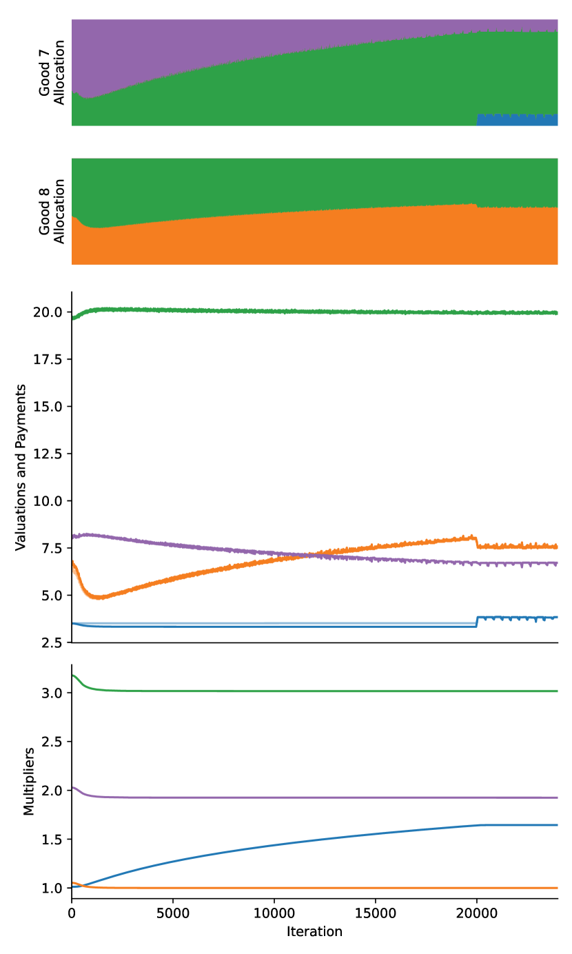
Figure 1: An instance of non-monotonicity.

If an auto-bidder lowers its multiplier, it will definitely win no more value immediately. However, other bidders will react to this change and the market will shift to a new equilibrium. Below we demonstrate such an example of transition in detail.

The market consists of 5 bidders and 10 goods. Figure 1 shows the dynamics after the change of tROI (technically tCPA) of some bidder at the old equilibrium, with time going by from left to right. Bidders are denoted by their colors in the figure. Only 4 bidders are plotted since the rest one wins nothing in both the old and the new equilibrium. During the transition, only the allocation of good 7 and 8 changes, which are depicted in the top two subplots: the vertical length (relative to the total) denotes the average fraction of auctions won by the bidder within a moving window pivoted at each time step. In the third subplot, we simultaneously draw the curves for valuations and payments. For bidders other than Blue, their ROI-constraints are always (almost) binding and thus there is only a single curve for each color. A twin curve is visible for Blue, whose payment (real line) is slightly less than valuation (translucent line) before around 20000 time steps, and as a result, Blue keeps raising its multiplier as shown in the fourth subplot.

At time 0, our manipulator Orange changes its tCPA to 0.95 of the original, resulting in a valuation profile $v^{\prime}$ such that $v_{Orange,j}^{\prime}=0.95v_{Orange,j},\forall j$. Each bidder applies the iterative method (Appendix H.2) to optimize its utility. Recall that, if the current ROI (aggregated over a moving window of recent rounds) is too high, the algorithm will lower its multiplier, and vice versa. To make the transition smooth, $\alpha_{Orange}$ is divided by $0.95$ right after the tCPA modification, which keeps the fine-grained bids of Orange unchanged at the moment. $\alpha_{Orange}=1$ at the old equilibrium and good 8 is the only good of which Orange wins a positive fraction.

Orange initiates the transition by lowering $\alpha_{Orange}$, since its ROI-constraint is now violated after its update of tCPA. However, Green does not want to win good 8 completely, otherwise its ROI-constraint will also be violated. So Green lowers its multiplier, as well, which further triggers the same behavior for Purple. As a result, Orange, Green and Purple reach an almost perfect coordination where the multiplicative ratios among their multipliers remain nearly constant all the way through the transition, as can also be seen from the fact that Purple and Green always tie for good 7, and Orange and Green always tie for good 8.

Blue’s allocation keeps unchanged for the first 20000 time steps. But it pays less due to the lowered second prices set by the other three and therefore tries to win more goods by gradually raising its multiplier. During the process, Purple and Green pay more for goods whose second prices are set by Blue, and thus they have to give up goods of which they are one of the tied winners (these goods have the lowest marginal ROIs): Purple gives up good 7 to Green, and Green wins more good 7 but loses good 8 to balance the deficit, which contributes to the success of the manipulation of Orange. In the end, Blue takes a fraction of good 7 away from Green to bind its ROI-constraint, and Green compensates this by taking a fraction of good 8 from Orange. Nonetheless, Orange still benefits from lowering its tCPA.

I.2 Competition among Sellers

It is not hard to see that, when bidders adjust bids based on the overall performance across the platform (a common practice in industry), there might be interference among different ad networks. To see this quantitatively, we take bidding data of two ad networks within the same platform during the same time period as the valuation profile, which consists of 59330 bidders and 222791 goods. We will apply different reserve pricing strategies to only one of the ad networks, and observe the treatment effects on both.

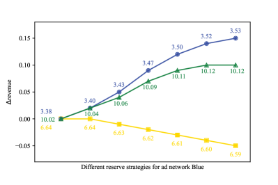
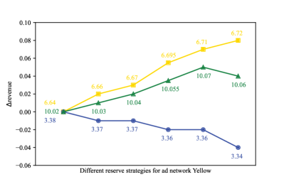
Figure 2: Ad network Blue (left) and Yellow (right) apply different reserve strategies to themselves, respectively.

The results are given in Figure 2. Ad networks are denoted by colors Blue and Yellow, and the platform is their sum Green = Blue + Yellow. Data points are translated vertically to better compare the net treatment effects, with absolute magnitudes annotated alongside. In the left plot, Blue applies different reserve pricing strategies to goods of its own. As its revenue increases, the platform also benefits but at a slower rate since Yellow is hurt. In particular, Blue’s revenue could continue to rise while the platform’s keeps flat, which means the revenue it gained comes from pure cannibalization. The results of the right plot are even worse, as the optimal strategy for Yellow does not align with the optimal one for the platform.

I.3 Approximate First Price Equilibrium in Second Price Markets

In the non-monotonicity example, if it were able to bid arbitrarily, Orange could secure good 8 in whole by raising its bids for goods other than 8, such that opponents, particularly Green, would have to pay more and retreat from the competition for good 8. Though multiplicative pacing is always enough to give a best response from hindsight, bidders have incentives to deviate from it, especially for those at a disadvantage at equilibrium (e.g., Orange has the unique highest valuation for good 8, but only wins a fraction of it; similarly for each pair of variable bidders in the proof of APX-hardness, see Appendix G). If all bidders are fully strategic, the line between first and second price may be blurred:

Proposition 2.

Suppose that each bidder $i$ can bid arbitrary $b_{i,j}$ for every good $j$. Then there is an equilibrium where $b_{i,j}=\max_{k}v_{k,j},\forall i,j$ and the good is freely shared among those bidders with $v_{i,j}=\max_{k}v_{k,j}$ at a price of $\max_{k}v_{k,j}$.

If a first price auction is used, no auto-bidding is needed (see Appendix L) and the allocation and payment is exactly the same as described above. Since the first-best revenue is achieved at this equilibrium, sellers have the incentive to (approximately) do so, and we will illustrate below that this is essentially what was done by Deng et al. (2021); Balseiro et al. (2021b).

With ROI-constraints in place, welfare serves as an upper bound for revenue. As goods are sold to bidders with lower valuations, the upper bound decreases. If bidders’ ROI-constraints are binding, the upper bound directly translates to revenue. Intuitively, Deng et al. (2021) try to prevent goods from being allocated to low-value bidders by adding an additive boosts that enlarges the differences of (boosted) valuations. Bidders with lower valuations would have to bid even higher to win (and they will always attempt to do so until binding their ROI-constraints), which could generally elevate the bid landscape and clearing prices.

Additive boost alone is not enough since it could lower the prices of goods sold to bidders with the highest values. Deng et al. (2021) did observe a decrease of revenue when boosts are excessively large (while the welfare still increases). Balseiro et al. (2021b) fix this with reserve prices, which not only increases the upper bound, but also directly provides a lower bound to avoid cheap sales.

Deng et al. (2021); Balseiro et al. (2021b) try to maintain the single-round IC property by imposing that the boosts and reserve prices should be generated from a highly accurate signal on the true (tROI-discounted) valuations independently of behaviors of both auto-bidders and advertisers. However, if the seller has access to such signals, there is almost no private information left to be elicited from advertisers. In this case, IC of even the advertiser-game matters little, let alone individual auctions. In essence, reserve prices behave just like a proxy bidder for the seller. With more accurate signals, it produces an outcome more similar to the one in Proposition 2. Boosts effectively does a similar job (though in a less direct manner), where each bidder faces a more competitive environment in auctions it values less than some opponent.

Appendix J Utility Instability for Advertisers

In this section, we investigate the utility instability problem through an extensive set of experiments. For equilibrium multiplicity, we generate 5 synthetic instances for each combination of type, distribution and market sizes. We have three types named complete, sampled and correlated, and either of the first two comes with a lognormal or uniform distribution (and will be called, e.g., complete lognormal) while correlated ones are parameterized by $\sigma$ that characterizes the intensity of competition. See Appendix H.3 on how they are generated. Instances of small sizes have $n=10,m=14$ and are solved using MIBLP, and moderate sizes have $n=50,m\in\{100,200,300\}$ and solved using the iterative method. For valuation sensitivity, instances are constructed by modifying the same base realistic instance, which consists of 85596 bidders, 3118648 goods and 14967663 non-zero $v_{i,j}$.

J.1 Equilibrium Multiplicity

In this section, the gap of bidder $i$ is measured as “the difference between the maximum and minimum values received by bidder $i$ in any equilibrium” divided by “the maximum value received by bidder $i$ in any equilibrium.” Bidders winning nothing in every equilibrium will not be considered.

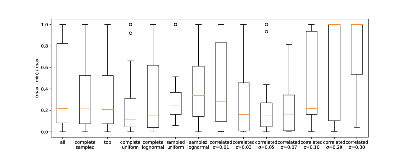
Figure 3: Gap distribution of small instances.

Experiment results of small instances are given in Figure 3. Over all small instances (the first box plot), more than half of bidders have a gap of more than 20%, and more than a quarter have a gap more than 80%. Even though many extreme cases are contributed by correlated instances, there is still more than a quarter of bidders have a gap of more than 50% for complete and sampled instances (the second box plot). We also check the gap distribution for the top 3 bidders of each instance (the third box plot), measured by the acquired value if first price auction is used (to make the ranking unique). They do perform better than the rest, but not much.

The gap distributions differ across classes of instances, with lognormal generally worse than uniform, sampled worse than complete. Correlated instances exhibit a U-shape w.r.t. $\sigma$, with large gap for both highly intense and sparse competition, and relatively small gap for middle ones. Nonetheless, at least a quarter of bidders always suffer a gap of about 30%, and there are almost always some unlucky bidders that win something in an equilibrium, but lose completely in another.

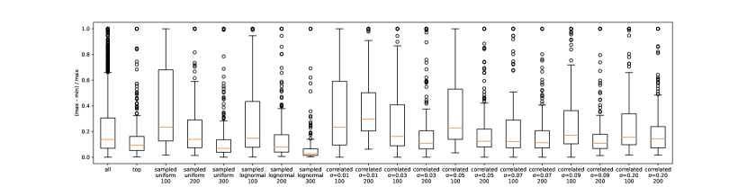
Figure 4: Gap distribution of moderate instances.

The situation improves for moderate instances, as shown in Figure 4. We can actually observe a clear trend where the gap distribution contracts as the number of goods increases. However, large gaps still happen a lot. Note that, even for instances of the same type and distribution, different sizes may also give quite distinct market structures. For an evidence, fixing $n=50$, if $m=100$, no more than 40 bidders on average could win something in at least one equilibrium. This number increases to around 45 for 200 goods, and almost 50 for 800 goods (not in the figure).

J.2 Valuation Sensitivity

We examine sensitivity of two types, one from an individual’s point of view, and the other from the market’s. The left plot of Figure 5 consists of two parts: the central box plot and the rest, each corresponding to one type of sensitivity.

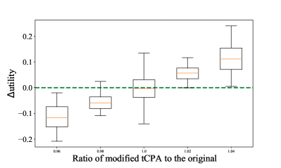
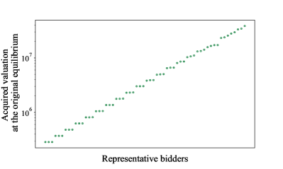
Figure 5: (Left) Change of utilities after adding noise. Outliers beyond whiskers are excluded. (Right) Selected bidders’ acquired valuations in the original equilibrium, which are made distributed evenly in the log scale.

For the four non-central box plots, each time we choose a bidder (based on their acquired valuations; see the right subplot of Figure 5) whose tCPA is changed to $x\in\{0.96,0.98,1.02,1.04\}$ times the original. First, we find that non-monotonicity still exists, as shown by the whisker above zero for $x=0.98$. Second, it holds for a significant portion of bidders that their utilities are quite sensitive to tCPAs. A quarter of bidders can gain or lose more than 15% of its value by making only a change of 4% of its tCPA. In the extreme case, a 4% change can bring 45% gain or 46% loss.

For the central box plot, we randomly generate 10 modified instances, each of which is constructed by flipping a fair coin for every bidder and adjusting its tCPA to either 0.99 or 1.01 times the original accordingly. We only focus on the top 4000 bidders measured on the acquired valuations in the original equilibrium. The gap distribution seems more stable than changing tCPA individually, but it features more extreme cases: about 3% of (bidder, modification) pairs have a gap of more than 20%, and more than 0.5% have a gap of more than 50%.

It is worth noting that markets with budget-constrained value-maximizers (in both first and second price auction) are completely insensitive to this kind of perturbation that scales a bidder’s valuation by a uniform factor. It has indeed been observed in practice that budget-constrained value-maximizing campaigns outperform ROI-constrained ones in stability.

J.3 Discussions

When will the utility become more robust against equilibrium selection? As implied by our hardness results (Appendix G), it is generally hard to compute how unstable the utility of each bidder is. Based on the U-shape results of small correlated instances, we hypothesize that: (1) When the competition is intense, the boundary between win and loss becomes narrow; when competition is sparse, the winner gains a large value surplus if the opponents’ multipliers are low. In both cases, it is more profitable to commit a large multiplier to claim the high ground in the competition and thwart the opponents. (2) With a moderate variance, the winner does not possess a large surplus even if multipliers of opponents stay at 1, and no one can suppress others easily. In this case, valuations are distributed more evenly across bidders and the utility becomes more stable.

An even value distribution across bidders, or a larger number of competitive bidders does seem to bring more stability with respect to equilibrium multiplicity, as further supported by the results of moderate instances, where utility becomes more stable as the number of goods increases but the competition for each good remains intact. Intuitively, with more competitive bidders, they clamp each other together to form a more stable structure. However, in this case the market may be more sensitive to the inputs, as shown by the realistic instances.

Why does duplication work in practice? Utility instability has been widely observed in practice. Advertisers have found a simple countermeasure, which is to create many campaigns with approximately the same configuration. Platforms will typically prevent auto-bidders of the same advertiser from competing with each other. Then with more campaigns, the instability of valuation prediction and equilibrium selection could be better neutralized, and the aggregate performance could be smoother. Our method to find multiple equilibria with the iterative method (Appendix H.2) is actually motivated by the real-world observation that, at the beginning of a campaign’s life, the prediction is more noisy, and duplication will effectively drive up the bid.

Duplication is annoying for platforms since it imposes an extra burden on the system but adds almost nothing informative and valuable. Some platforms have restricted the maximum number of campaigns that can be run simultaneously by a single advertiser, and algorithms have been implemented to cluster and prune similar campaigns. To alleviate instability, platforms could actively boost or suppress bidders (as in our experiments) based on their historic performance. Note that, when we apply the Bernoulli $\pm 0.01$ noise to valuations, the total revenue remains stable, with a gap between the worst and best only $0.15\%$. Even when we increase the noise magnitude to 0.02, the gap is just $0.22\%$. Hence such strategies will not sacrifice the revenue of the platform.

Appendix K A/B Testing for Platforms

In this section, we investigate the interference in A/B testing of auction markets.

User-side experiments are performed by applying the treatment variant to $r$ percents of auctions ($x$-axis in Figure 6; for each $r$, results are aggregated over several random partitions to make sure that the biases are not from non-homogeneous user-splitting) uniformly at random and the control variant to the rest. We will measure the ground-truth treatment effect (dashed lines in Figure 6) by computing the ratio of “metrics when applying the treatment variant to all the auctions” over “metrics when applying the control variant to all.” The A/B tested treatment effect (real lines in Figure 6) is simply the ratio of metrics between experiment groups. We use realistic bidding data and include the additive boost mechanism. In the first experiment (left of Figure 6), the treatment group is assigned a boost of magnitudes $c_{i,j}=0.05v_{i,j}$ and the control group has no boost. In the second, we use the boost used online for the control group, and half its value for the treatment. The online boost is used in the real world as a measure of long-term utility to the platform. As we can see from Figure 6 that, when it is halved, the immediate revenue is indeed increased by sacrificing long-term utilities, and thus its weight should be carefully configured to optimize the overall financial consequences.

In real-world markets, it is important for a bidding algorithm to handle the uncertainty of the environment in practice. Therefore, to better resemble the situation where ad-side A/B testing is used in the real world, here we deviate a little from the deterministic model to a stochastic one (but the result can still be explained largely within our framework). Each market instance consists of 200 bidders and $400\times 1000$ goods. Auctions do not happen simultaneously, but arrive one-by-one. Before each auction $j$, each bidder $i$ has an unbiased prior estimation $v_{i,j}$ for the value of good. In the simulation, $v_{i,j}$ is drawn i.i.d. from the distribution $\min\left(\left|X\right|,1.0\right)),X\sim\text{Normal}(0,0.1)$. The value received by bidder $i$ after winning is not $v_{i,j}$, but randomly drawn from $\text{Bernoulli}(v_{i,j})$ (mimicking conversions of discrete types in practice). For each bidder, its bid $b_{i,j}=\alpha_{i}v_{i,j}$ is still given by a multiplicative pacing strategy, where $\alpha_{i}$ is controlled by a PID controller (see the work by Zhang et al. (2016)) that adjusts the multiplier after every 1000 auctions to optimize the acquired realized value subject to that the ROI-constraint should be satisfied approximately. PID controllers have 4 parameters and we will run A/B tests for different pairs of parameter configurations (100 bidders for each group, and bidders in the same group share the same parameter configuration).

Ad-side experiment groups are evaluated on two classes of metrics: efficiency and stability, both are widely used in practice. Though the market becomes stochastic and dynamic, it is easy to see that, in the long round, multipliers should still converge to the auto-bidding equilibrium for the market with deterministic valuations $\{v_{i,j}\}$. Efficiency metrics (the revenue and welfare of the platform) are meant to measure how good the resulted equilibrium is economically for the platform. On the other hand, since $\{v_{i,j}\}$ is only an expectation and the problem is online, ROI-constraints may not always be perfectly satisfied. So we use the success rate (the proportion of revenue generated from bidders ending with a ROAS between 0.975 to 1.025) and failure rate (the proportion of revenue from bidders with ROAS above 1.025) to quantify how well the PID controllers handle the uncertainty for advertisers. Each pair of parameter configurations is evaluated through A/B testing over 100 market instances, and statistical test is performed with respect to each metrics to determine whether the treatment variant performs significantly better or worse than the control. The ground-truth is measured by applying the configuration to all bidders and aggregate metrics over 100 market instances.

K.1 Simulation Results

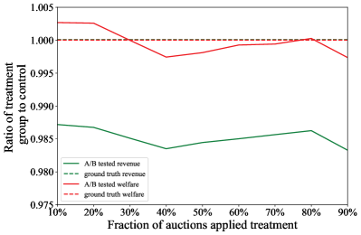
Figure 6: Results of user-side experiments.

User-side experiments.

Figure 6 depicts results of user-side experiments for two pairs of treatment/control variants. In the left, the ground-truth treatment effect is nearly zero, but A/B testing shows that we may lose more than 1% revenue. Welfare seems more robust in this case, but it is also inconsistent and has a gap of more than 0.5% between the most optimistic and pessimistic estimations. In the second experiment, welfare deviates worse than revenue, with a maximum of bias more than 1%. Note that a bias of 0.5% is large enough to affect practitioners’ decisions (e.g., the minimum detectable treatment effect in the platform from which our data are taken is roughly at the same scale), and if multiple objectives are to be weighted, the requirement for accuracy is even stricter. Based on our observation over some more experiments not displayed here, we find that welfare is generally more robust than revenue. If naive A/B testing is the only option, welfare seems to be more reliable as an overall evaluation metrics.

naive vs. ground truth	setup	revenue	welfare	success rate	failure rate
overestimate efficiency wrong stability	ground truth	+1.21%*	+1.10%*	-3.96%*	+11.55%*
	naive	+13.18%*	+13.37%*	+2.76%*	-9.31%*
	boosted	+0.86%*	+0.91%*	-1.91%*	+4.60%*
wrong efficiency wrong stability	ground truth	-0.67%*	-0.76%*	+2.96%*	-2.10%
	naive	+3.12%*	+3.06%*	-0.67%	+3.33%
	boosted	-0.64%*	-0.73%*	+0.89%*	+0.86%
wrong efficiency wrong stability	ground truth	-0.29%*	-0.31%*	-3.56%*	+3.56%*
	naive	+13.49%*	+13.36%*	+5.28%*	-1.61%
	boosted	-0.24%*	-0.30%*	-4.84%*	+8.38%*

Table 8: Results of three groups of ad-side experiments. Each entry is calculated as the ratio of “metrics difference of the treatment variant to the control” over “the metrics of the control variant”. Asterisks indicate statistical significance. Note that a strategy with lower failure rate is considered better.

Ad-side experiments.

Examples with biases of different types are given in Table 8 (naive vs. ground truth). The bias is irregular as we can observe that there may be significant overestimation, or a worse variant may be measured as better, etc. In particular, in the third example, naive A/B tests tell us that the treatment variant beats the control in all metrics by a large margin, but if we apply it to all bidders, the resulted system would instead perform worse.

K.2 Explanations and A General Approach to Diagnosis and Design

During user-side A/B testing, the market is a mixture of treatment and control groups, and the resulted equilibrium multipliers are not equal (or even close) to those if either variant were applied counterfactually to all the auctions. The same argument can also explain the failure of ad-side A/B tests on measuring revenue and welfare. As for success and failure rate, the hypothesis is that, if a significantly more amount of auctions are won by one group (as is the case here), their received values would converge closer to the expectation and the environment becomes less uncertain and easier to deal with. All in all, in an A/B test, any experiment group (of either users or ads) faces a different competitive environment from the one in the counterfactual “B/B” or “A/A” test where both groups were assigned the same variant. Thus to reduce bias, a general principle is to make the experiment group behave (for each individual or at least the group as a whole) as if the other group is also assigned the same variant.

The principle might seem too general and it is not immediately clear how to achieve it, in particular in markets involving complex strategic behaviors. To make it applicable, we propose an approach using the concept of invariants. We start with identifying a metrics (the invariant) that should remain the same regardless of whether the treatment or control variant is applied. For naive tests, it serves as a signal that there may be bias if this metrics varies significantly across experiment groups. For example, the ROI-constraint should always be binding when aggregated across the market, but in Figure 6 the ratio of revenue over welfare for each group deviates significantly from 1. As for designing less-biased setups, we should try to restore the balance of the invariant. In retrospect, the work by Liu, Mao, and Kang (2020) is an instantiation of this approach for user-side experiments where the invariant is budget (of each advertiser), and Ha-Thuc et al. (2020) is one for non-auction markets with recommendation positions (occupied by each group as a whole) as the invariant.

For user-side experiments in our ROI-constrained markets, ROI simply serves as the invariant and we can assign an auto-bidder for each advertiser and each experiment group (instead of the whole market as more commonly done in practice). This computes the correct outcome in theory if there is a unique (and efficiently computable) equilibrium and the two experiment groups are perfectly homogeneous. For the less-studied ad-side experiments, we instantiate the approach with a new boosted design using the number of auctions won by each group on average as the invariant. To make it balanced, right after each episode (here 1000 auctions), a uniform additive boost $c$ for treatment group will be calculated in a counterfactual way such that, if it were applied to the treatment group in the last episode (i.e., if good $j$ were allocated to the bidder with highest $\alpha_{i}v_{i,j}+c_{i}$, where $c_{i}=c$ if $i$ is in treatment group, $c_{i}=0$ otherwise), goods would be split into two groups perfectly in proportion ($r$ percent of ads should win $r$ percent of auctions). The boosts will then be applied to the treatment group throughout the next episode.

Table 8 (boosted) shows that it works really well for these synthetic instances: it always gives the correct qualitative result (statistically better, worse, or insignificant) and it is also more accurate quantitatively, especially on revenue and welfare. As a comparison, we try to adapt the counterfactual design by Ha-Thuc et al. (2020) where treatment and control are applied to all bidders respectively to get two rankings, and then merge them to decide the winner. Ha-Thuc et al. (2020) (not designed for auctions) did not specify the payment rule, and we tried several alternatives but no one works: in the contrary, the number of auctions won by each group is more unbalanced and the bias is severely exaggerated.

Appendix L First Price versus Second Price: Theory and Beyond

First price auto-bidding equilibrium.

With first price auction, no auto-bidding is needed and the platform simply allocates goods to bidders with the highest (tROI-discounted) valuations, which are also charged as payments. Quasi-linear utility makes no difference for advertisers and it is a dominant strategy to report their tROIs truthfully. Even if they prefer spending less with the same acquired value, the incentive to deviate diminishes as the market becomes thicker. (This technically deviates from our auto-bidding model and we will characterize the equilibrium with this new utility model in Appendix M. Importantly, the equilibrium is still unique and always achieves the first-best welfare discounted by true tROIs.) First price auction does not provide advertisers an ex-post optimal outcome. However, advertisers should happily accept the outcome since it is still fair in the sense that it resembles closely to the classic competitive equilibrium in Fisher markets.

Besides economic efficiency, fairness and strategyproofness, first price auction also dominates in almost all the other aspects we study in this paper: (1) the market outcome is unique; (2) computation is trivial; (3) ROI-monotonicity; (4) no interference among sub-markets; (5) competition is direct and local; even if the competition is so intense that the utility becomes unstable, it can easily be smoothed by actively applying small perturbations or probabilistic allocations (Borgs et al. 2007). It shares with second price auction the problem of biases in ad-side A/B testing since it is rooted in the setup itself, irrelevant to auction formats. Budget-constrained markets share similar results (Conitzer et al. 2022a): (1) the equilibrium is unique; (2) computation is convex and tractable; (3) budget-monotonicity. Since budget should still be paced, there remains interference among sub-markets and the competition is less direct than within ROI-constrained markets. Nonetheless, with first price auction, the market is convex and more predictable, in contrast to the complex combinatorial structure of second price auction that is hard to tackle as shown both here and by Conitzer et al. (2022b).

Possible rationale behind Google’s partial shift from second to first price.

We have given much mathematical evidence to establish the dominance of first price auction over second price within our auto-bidding market model. But once an advertiser could submit tROIs (or budgets) for even just two different sub-markets of the platform, it opens opportunities for strategic manipulations and the aforementioned properties technically break. This, however, does not mean that second price auction could immediately regain the upper hand as in the single-item regime, either. Though it cannot be easily stated and verified in a fully rigorous manner, it is reasonable to give the following hypothesis: with advertisers having access to a wider range of heterogeneous sub-markets, second price auction could reduce strategic behaviors more effectively and bring better market outcomes; conversely, if optional sub-markets are coarse-grained and advertisers do not have enough knowledge to differentiate them, the market could still be well captured by our model and first price auction mostly retains its dominant position.

As for Google, the most distinctive feature that sets Search and Shopping apart from Content, Video and Games is the way in which items (both sponsored and non-sponsored) are distributed to users. For the former, users typically come with a clear intent expressed through the keywords they input. Even though there are still variations, keywords largely determine the items to be recommended and thus each keyword characterizes a sub-market of which advertisers have a fairly good understanding. In contrast, users’ general interests are highly personal. A platform can learn a lot from users’ interactions with the items, but the disclosure of such information is extremely selective for both economic and privacy concerns. In this case, the platform knows much more than advertisers (and even users themselves), and they typically cannot (and will not) manipulate much to optimize every penny they spend in this more centralized market.

Appendix M First Price Meta-game Equilibrium with Frugal ROI-constrained Value-maximizers

Let $(v_{1},p_{1})$ and $(v_{2},p_{2})$ be two outcomes where $v_{k}$ is the total value received by some bidder $i$ and $p_{k}$ the payment. If $i$ is a frugal ROI-constrained value-maximizing bidder, it strictly prefers $(v_{1},p_{1})$ to $(v_{2},p_{2})$ if and only if (1) $v_{1}>v_{2}$ or (2) $v_{1}=v_{2}$ and $p_{1}<p_{2}$.

In the main text we assume a tROI of zero. Here we will consider advertisers’ behavior in the meta-game, and we will use $v_{i,j}$ to denote the valuation of advertiser $i$ to good $j$ discounted by $i$’s true tROI rather than the reported. For simplicity we also assume $\operatornamewithlimits{arg\,max}_{i}v_{i,j}$ is unique for every good $j$.

Definition 3 (First Price Meta-game Equilibrium).

The equilibrium $(x,p)$ consists of allocation $x\in\{0,1\}^{n\times m}$ and payment $p\in[0,+\infty)^{n}$ such that

• goods go to the bidder with the highest true tROI-discounted valuation: $x_{i,j}=1$ if and only if $i=\operatornamewithlimits{arg\,max}_{k}v_{k,j}$, $\forall j$;

• bidder pays its total acquired valuation discounted by the minimum tROI required to win the set of goods currently allocated:

  $$p_{i}=\alpha_{i}\sum_{j}v_{i,j}x_{i,j}\text{ where }\alpha_{i}=\max_{k,j:x_{i,j}=1,k\neq i}\frac{v_{k,j}}{v_{i,j}}.$$

At equilibrium, each advertiser effectively bids $b_{i,j}=\alpha_{i}v_{i,j}$ in each individual first price auction and ties are broken in favor of the one with the highest (true tROI-discounted) value. If $i$ bids with a multiplier less than $\alpha_{i}$, some other bidder could bid truthfully and win an item that is currently allocated to $i$.

The equilibrium is unique and achieves first-best welfare (discounted by true tROIs). It is not clear how to compare the revenue with second price auction, wherein the behaviors of both advertisers and auto-bidders are highly unpredictable.

References

- Aggarwal, Badanidiyuru, and Mehta (2019) Aggarwal, G.; Badanidiyuru, A.; and Mehta, A. 2019. Autobidding with constraints. In International Conference on Web and Internet Economics, 17–30. Springer.
- Akbarpour and Li (2020) Akbarpour, M.; and Li, S. 2020. Credible auctions: A trilemma. Econometrica, 88(2): 425–467.
- Ausiello et al. (2012) Ausiello, G.; Crescenzi, P.; Gambosi, G.; Kann, V.; Marchetti-Spaccamela, A.; and Protasi, M. 2012. Complexity and approximation: Combinatorial optimization problems and their approximability properties. Springer Science & Business Media.
- Babaioff et al. (2021) Babaioff, M.; Cole, R.; Hartline, J.; Immorlica, N.; and Lucier, B. 2021. Non-Quasi-Linear Agents in Quasi-Linear Mechanisms. In 12th Innovations in Theoretical Computer Science Conference (ITCS 2021). Schloss Dagstuhl-Leibniz-Zentrum für Informatik.
- Balseiro et al. (2021a) Balseiro, S.; Deng, Y.; Mao, J.; Mirrokni, V.; and Zuo, S. 2021a. The Landscape of Auto-Bidding Auctions: Value Versus Utility Maximization. Available at SSRN 3785579.
- Balseiro et al. (2021b) Balseiro, S.; Deng, Y.; Mao, J.; Mirrokni, V.; and Zuo, S. 2021b. Robust Auction Design in the Auto-bidding World. Advances in Neural Information Processing Systems, 34.
- Balseiro et al. (2021c) Balseiro, S.; Kim, A.; Mahdian, M.; and Mirrokni, V. 2021c. Budget-Management Strategies in Repeated Auctions. Operations Research.
- Balseiro and Gur (2019) Balseiro, S. R.; and Gur, Y. 2019. Learning in repeated auctions with budgets: Regret minimization and equilibrium. Management Science, 65(9): 3952–3968.
- Balseiro, Lu, and Mirrokni (2022) Balseiro, S. R.; Lu, H.; and Mirrokni, V. 2022. The best of many worlds: Dual mirror descent for online allocation problems. Operations Research.
- Blake and Coey (2014) Blake, T.; and Coey, D. 2014. Why marketplace experimentation is harder than it seems: The role of test-control interference. In Proceedings of the fifteenth ACM conference on Economics and computation, 567–582.
- Borgs et al. (2007) Borgs, C.; Chayes, J.; Immorlica, N.; Jain, K.; Etesami, O.; and Mahdian, M. 2007. Dynamics of bid optimization in online advertisement auctions. In Proceedings of the 16th international conference on World Wide Web, 531–540.
- Charles et al. (2013) Charles, D.; Chakrabarty, D.; Chickering, M.; Devanur, N. R.; and Wang, L. 2013. Budget smoothing for internet ad auctions: a game theoretic approach. In Proceedings of the fourteenth ACM conference on Electronic commerce, 163–180.
- Chen, Deng, and Teng (2009) Chen, X.; Deng, X.; and Teng, S.-H. 2009. Settling the complexity of computing two-player Nash equilibria. Journal of the ACM (JACM), 56(3): 1–57.
- Chen, Kroer, and Kumar (2021a) Chen, X.; Kroer, C.; and Kumar, R. 2021a. The Complexity of Pacing for Second-Price Auctions. arXiv preprint arXiv:2103.13969.
- Chen, Kroer, and Kumar (2021b) Chen, X.; Kroer, C.; and Kumar, R. 2021b. Throttling equilibria in auction markets. arXiv preprint arXiv:2107.10923.
- Chu et al. (2020) Chu, H.; Trenkle, J. M.; Tangirala, S.; and Wang, A. 2020. Using a PID controller engine for controlling the pace of an online campaign in realtime. US Patent 10,878,448.
- Conitzer et al. (2022a) Conitzer, V.; Kroer, C.; Panigrahi, D.; Schrijvers, O.; Stier-Moses, N. E.; Sodomka, E.; and Wilkens, C. A. 2022a. Pacing equilibrium in first price auction markets. Management Science, 68(12): 8515–8535.
- Conitzer et al. (2022b) Conitzer, V.; Kroer, C.; Sodomka, E.; and Stier-Moses, N. E. 2022b. Multiplicative pacing equilibria in auction markets. Operations Research, 70(2): 963–989.
- Dasgupta and Tsui (2004) Dasgupta, S.; and Tsui, K. 2004. Auctions with cross-shareholdings. Economic Theory, 24(1): 163–194.
- Debreu (1952) Debreu, G. 1952. A social equilibrium existence theorem. Proceedings of the National Academy of Sciences, 38(10): 886–893.
- Deng et al. (2022) Deng, Y.; Mao, J.; Mirrokni, V.; Zhang, H.; and Zuo, S. 2022. Efficiency of the first-price auction in the autobidding world. arXiv preprint arXiv:2208.10650.
- Deng et al. (2021) Deng, Y.; Mao, J.; Mirrokni, V.; and Zuo, S. 2021. Towards Efficient Auctions in an Auto-bidding World. In Proceedings of the Web Conference 2021, 3965–3973.
- Despotakis, Ravi, and Sayedi (2021) Despotakis, S.; Ravi, R.; and Sayedi, A. 2021. First-price auctions in online display advertising. Journal of Marketing Research, 58(5): 888–907.
- Fan (1952) Fan, K. 1952. Fixed-point and minimax theorems in locally convex topological linear spaces. Proceedings of the National Academy of Sciences of the United States of America, 38(2): 121.
- Filos-Ratsikas et al. (2021) Filos-Ratsikas, A.; Giannakopoulos, Y.; Hollender, A.; Lazos, P.; and Poças, D. 2021. On the complexity of equilibrium computation in first-price auctions. In Proceedings of the 22nd ACM Conference on Economics and Computation, 454–476.
- Gao and Kroer (2020) Gao, Y.; and Kroer, C. 2020. First-order methods for large-scale market equilibrium computation. arXiv preprint arXiv:2006.06747.
- Glicksberg (1952) Glicksberg, I. L. 1952. A further generalization of the Kakutani fixed point theorem, with application to Nash equilibrium points. Proceedings of the American Mathematical Society, 3(1): 170–174.
- Golrezaei, Lobel, and Paes Leme (2021) Golrezaei, N.; Lobel, I.; and Paes Leme, R. 2021. Auction design for ROI-constrained buyers. In Proceedings of the Web Conference 2021, 3941–3952.
- Gürtler and Gürtler (2012) Gürtler, M.; and Gürtler, O. 2012. Inequality aversion and externalities. Journal of Economic Behavior & Organization, 84(1): 111–117.
- Ha-Thuc et al. (2020) Ha-Thuc, V.; Dutta, A.; Mao, R.; Wood, M.; and Liu, Y. 2020. A counterfactual framework for seller-side a/b testing on marketplaces. In Proceedings of the 43rd International ACM SIGIR Conference on Research and Development in Information Retrieval, 2288–2296.
- Holtz et al. (2020) Holtz, D.; Lobel, R.; Liskovich, I.; and Aral, S. 2020. Reducing interference bias in online marketplace pricing experiments. Available at SSRN 3583836.
- Johari, Li, and Weintraub (2020) Johari, R.; Li, H.; and Weintraub, G. 2020. Experimental Design in Two-Sided Platforms: An Analysis of Bias. In Proceedings of the 21st ACM Conference on Economics and Computation, 851–851.
- Kagel and Levin (2011) Kagel, J. H.; and Levin, D. 2011. Auctions: A survey of experimental research, 1995-2010. Handbook of experimental economics, 2: 563–637.
- Karande, Mehta, and Srikant (2013) Karande, C.; Mehta, A.; and Srikant, R. 2013. Optimizing budget constrained spend in search advertising. In Proceedings of the sixth ACM international conference on Web search and data mining, 697–706.
- Karrer et al. (2021) Karrer, B.; Shi, L.; Bhole, M.; Goldman, M.; Palmer, T.; Gelman, C.; Konutgan, M.; and Sun, F. 2021. Network experimentation at scale. In Proceedings of the 27th ACM SIGKDD Conference on Knowledge Discovery & Data Mining, 3106–3116.
- Kimbrough and Reiss (2012) Kimbrough, E. O.; and Reiss, J. P. 2012. Measuring the distribution of spitefulness.
- Kitts et al. (2017) Kitts, B.; Krishnan, M.; Yadav, I.; Zeng, Y.; Badeau, G.; Potter, A.; Tolkachov, S.; Thornburg, E.; and Janga, S. R. 2017. Ad Serving with Multiple KPIs. In Proceedings of the 23rd ACM SIGKDD International Conference on Knowledge Discovery and Data Mining, 1853–1861.
- Leme, Syrgkanis, and Tardos (2012) Leme, R. P.; Syrgkanis, V.; and Tardos, É. 2012. Sequential auctions and externalities. In Proceedings of the twenty-third annual ACM-SIAM symposium on Discrete Algorithms, 869–886. SIAM.
- Liaw, Mehta, and Perlroth (2022) Liaw, C.; Mehta, A.; and Perlroth, A. 2022. Efficiency of non-truthful auctions under auto-bidding. arXiv preprint arXiv:2207.03630.
- Liu, Mao, and Kang (2020) Liu, M.; Mao, J.; and Kang, K. 2020. Trustworthy online marketplace experimentation with budget-split design. arXiv preprint arXiv:2012.08724.
- Lo et al. (2020) Lo, C.; De Longueau, E.; Saha, A.; and Chatterjee, S. 2020. Edge formation in Social Networks to Nurture Content Creators. In Proceedings of The Web Conference 2020, 1999–2008.
- Maehara et al. (2018) Maehara, T.; Narita, A.; Baba, J.; and Kawabata, T. 2018. Optimal Bidding Strategy for Brand Advertising. In IJCAI, 424–432.
- Morishita et al. (2020) Morishita, G.; Abe, K.; Ogawa, K.; and Kaneko, Y. 2020. Online Learning for Bidding Agent in First Price Auction. In Workshop on Reinforcement Learning in Games in Thirty-Fourth AAAI Conference on Artificial Intelligence.
- Paes Leme, Sivan, and Teng (2020) Paes Leme, R.; Sivan, B.; and Teng, Y. 2020. Why do competitive markets converge to first-price auctions? In Proceedings of The Web Conference 2020, 596–605.
- Papadimitriou and Peng (2021) Papadimitriou, C.; and Peng, B. 2021. Public goods games in directed networks. In Proceedings of the 22nd ACM Conference on Economics and Computation, 745–762.
- Rabin (1993) Rabin, M. 1993. Incorporating fairness into game theory and economics. The American economic review, 1281–1302.
- Ren et al. (2017) Ren, K.; Zhang, W.; Chang, K.; Rong, Y.; Yu, Y.; and Wang, J. 2017. Bidding machine: Learning to bid for directly optimizing profits in display advertising. IEEE Transactions on Knowledge and Data Engineering, 30(4): 645–659.
- Rubinstein (2018) Rubinstein, A. 2018. Inapproximability of Nash Equilibrium. SIAM Journal on Computing, 47(3): 917–959.
- Smirnov, Lu, and Lee (2016) Smirnov, Y.; Lu, Q.; and Lee, K.-c. 2016. Online ad campaign tuning with pid controllers. US Patent App. 14/518,601.
- Tu et al. (2019) Tu, Y.; Lo, C.; Yuan, Y.; and Chatterjee, S. 2019. Feedback shaping: A modeling approach to nurture content creation. In Proceedings of the 25th ACM SIGKDD International Conference on Knowledge Discovery & Data Mining, 2241–2250.
- Tunuguntla and Hoban (2021) Tunuguntla, S.; and Hoban, P. R. 2021. A near-optimal bidding strategy for real-time display advertising auctions. Journal of Marketing Research, 58(1): 1–21.
- Wu et al. (2018) Wu, D.; Chen, X.; Yang, X.; Wang, H.; Tan, Q.; Zhang, X.; Xu, J.; and Gai, K. 2018. Budget constrained bidding by model-free reinforcement learning in display advertising. In Proceedings of the 27th ACM International Conference on Information and Knowledge Management, 1443–1451.
- Xu et al. (2018) Xu, J.; Lee, K.-c.; Li, W.; Qi, H.; and Lu, Q. 2018. Pacing control for online ad campaigns. US Patent 10,068,247.
- Yang et al. (2019) Yang, X.; Li, Y.; Wang, H.; Wu, D.; Tan, Q.; Xu, J.; and Gai, K. 2019. Bid optimization by multivariable control in display advertising. In Proceedings of the 25th ACM SIGKDD International Conference on Knowledge Discovery & Data Mining, 1966–1974.
- Zhang et al. (2016) Zhang, W.; Rong, Y.; Wang, J.; Zhu, T.; and Wang, X. 2016. Feedback control of real-time display advertising. In Proceedings of the Ninth ACM International Conference on Web Search and Data Mining, 407–416.