Annihilation of Spurious Minima
in Two-Layer ReLU Networks

Abstract

We study the optimization problem associated with fitting two-layer ReLU neural networks with respect to the squared loss, where labels are generated by a target network. Use is made of the rich symmetry structure to develop a novel set of tools for studying the mechanism by which over-parameterization annihilates spurious minima. Sharp analytic estimates are obtained for the loss and the Hessian spectrum at different minima, and it is proved that adding neurons can turn symmetric spurious minima into saddles; minima of lesser symmetry require more neurons. Using Cauchy’s interlacing theorem, we prove the existence of descent directions in certain subspaces arising from the symmetry structure of the loss function. This analytic approach uses techniques, new to the field, from algebraic geometry, representation theory and symmetry breaking, and confirms rigorously the effectiveness of over-parameterization in making the associated loss landscape accessible to gradient-based methods. For a fixed number of neurons and inputs, the spectral results remain true under symmetry breaking perturbation of the target.

1 Introduction

An outstanding question in deep learning (DL) concerns the ability of simple gradient-based methods to successfully train neural networks despite the nonconvexity of the associated optimization problems. Indeed, nonconvex optimization landscapes may have spurious (i.e., non-global local) minima with large basins of attraction and this can cause a complete failure of these methods. Evidence suggests that this problem can be circumvented by the use of a large number of parameters in DL models. In view of the complexity exhibited by contemporary neural networks and the absence of suitable analytic tools, much recent research has focused on two-layer ReLU networks as a realistic starting point for a theoretical study [1, 2, 3, 4, 5, 6, 7]. The two-layer networks considered were typically of the form:

$$f({\bm{x}};W,\boldsymbol{\alpha})\coloneqq\boldsymbol{\alpha}^{\top}\!\varphi(W{\bm{x}}),\quad~{}W\in M(k,d),~{}\boldsymbol{\alpha}\in\mathbb{R}^{k},$$ (1)

where $\varphi(z)\coloneqq\max\{0,z\}$ is the ReLU function acting entrywise and $M(k,d)$ denotes the space of $k\times d$ matrices. In order to isolate the study of optimization-related obstructions due to nonconvexity from issues pertaining to the expressive power of two-layer networks, data has been often assumed to be fully realizable. This was further motivated by hardness results which indicated a strict barrier inherent to the explanatory power of distribution-free approaches operating in complete generality [8, 9, 10]. For the squared loss, the resulting, highly nonconvex, expected loss is

$$\mathcal{L}(W,\boldsymbol{\alpha})\coloneqq\frac{1}{2}\mathbb{E}_{{\bm{x}}\sim\mathcal{D}}\left[\Big{(}f({\bm{x}};W,\boldsymbol{\alpha})-f({\bm{x}};V,\boldsymbol{\beta})\Big{)}^{2}\right],$$ (2)

where $\mathcal{D}$ denotes a probability distribution over the input space, $W\in M(k,d)$, $\boldsymbol{\alpha}\in\mathbb{R}^{k}$ are the optimization variables, and $V\in M(d,d)$, $\boldsymbol{\beta}\in\mathbb{R}^{d}$ are fixed parameters.

The choice of the $d$-variate normal Gaussian distribution for the input distribution has drawn a considerable interest, e.g., [11, 12, 13, 14, 15, 16, 17]. Empirically, it has been observed that as the number of neurons $k$ increases, the loss of models obtained using stochastic gradient descent (SGD) under Xavier initialization [18] decreases (see [9, 19]). The objective of this work is to study the mathematical mechanism behind this fundamental phenomenon. Using ideas based on symmetry breaking (see Section 2), we are able to employ techniques from representation theory and algebraic geometry to study how the loss landscape is transformed when the number of neurons is increased. A key feature of our approach is the use of Puiseux series in $d$ and path based techniques. For example, we may define the spectrum of the Hessian as Puiseux series for real values of $d$ and so determine the values of $d$ (typically not integers) where eigenvalues change sign. These methods allow the proof of powerful analytic results: in this paper, we derive sharp analytic estimates of the loss and the Hessian spectrum at local minima allowing us to analyze the mechanism whereby spurious minima are annihilated when the number of neurons $k$ is increased. Our contributions can be summarized by

Theorem 1

(Informal) We describe several infinite families of spurious minima, partly characterized by their symmetry, and prove that:
$\bullet$ Adding rather few neurons can transform symmetric spurious minima into saddles.
$\bullet$ The Hessian spectrum remains extremely skewed with $\Theta(d)$ eigenvalues growing linearly with $d$, and $\Theta(kd)$ eigenvalues being $\Theta(1)$.
$\bullet$ Increasing the number of neurons adds $\Theta(d)$ descent directions in a $\Theta(d)$-dimensional subspace dictated by the symmetry structure (i.e., the isotypic decomposition) of the loss function.
$\bullet$ The loss remains (essentially) unchanged.

The formation of new decent directions allows gradient-based methods to escape spurious minima that exist in the original loss landscape ($k=d$), and so detect models of reduced loss. To indicate the subtly of the results given in Theorem 1, consider a family of spurious minima with symmetry $\Delta(S_{d-1}\times S_{1})$ (the type II family described in Section 3). Assume $k=d$. Spurious minima occur for $d\geq 6$. Adding one neuron results in these minima occurring for $d\geq 8$ — not promising. Adding two neurons annihilates all these spurious minima and creates no new spurious minima. The mechanism is finite, cannot be inferred from a limiting case, and persists under forced symmetry breaking, and so applies beyond symmetric targets. If instead we consider the unique family of spurious minima with isotropy $\Delta S_{d}$ (see Section 3), we find that adding just one neuron annihilates these spurious minima. This occurs through the appearance of a multiplicity $(d-1)$-eigenvalue associated to the standard representation of $S_{d}$ on ^d-1 (all other eigenvalues remain positive). More precisely, if $k=d$ there are 3 strictly positive Hessian eigenvalues associated to the standard representation of $S_{d}$, each with multiplicity $d-1$. Modulo $O(d^{-\frac{1}{2}})$ terms, they are $\frac{1}{4}-\frac{1}{2\pi},\frac{1}{4}$, and $\frac{d}{4}+\frac{1}{4}$. After the addition of one neuron ($k=d+1$), there are 4 Hessian eigenvalues associated to the standard representation of $S_{d}$ and, modulo $O(d^{-\frac{1}{2}})$ terms, these satisfy

$$\frac{d}{4}+\frac{1}{2},\frac{1}{4}-\frac{1}{2\pi},\frac{-1+\sqrt{5}}{4\pi}+\frac{1}{4}>0>\frac{-1-\sqrt{5}}{4\pi}+\frac{1}{4}.$$

This example highlights the special role that the standard representation plays in the annihilation of spurious minima (see Section 5 and the concluding remarks). The sharp estimates of the Hessian spectrum further demonstrate how symmetry breaking enables a complete characterization of the dynamics of gradient-based methods, locally, in the vicinity of symmetric critical points. The dependence of such methods on stability of critical points therefore indicates that attempts for a global theory should be preceded by a good description of the mechanism by which spurious minima transform into saddles—the aim of this work.

Next, we relate our results to the existing literature.

Annihilation of spurious minima on account of over-parameterization.

Existing methods for the analysis of optimization problem (2) include: mean-field [4], optimal transport [2], NTK [20, 21, 22] and the thermodynamic limit [5, 16, 23, 24]. These methods operate by passing to limiting regimes where the number of inputs or neurons is taken to infinity. A growing number of works has limited the explanatory power of such approaches [25, 26]. Approaches for addressing the loss landscapes in finite parameter regimes exist and include [6] which obtains several generalities on critical points, and [7] which studies conditions under which a single neuron can be added in contrived way so as to turn a given minimum in $M(d,d)$ into a saddle in $M(d+1,d)$. However, as shown in the present work, families of minima in $M(d+1,d)$ exist. Indeed, families of minima of lesser symmetry are shown to require at least two additional neurons before turning into saddles.

Symmetry breaking in nonconvex loss landscapes.

It has been recently found that the symmetry of spurious minima in optimization problem (2) break the symmetry of global minima [27] (see Section 2 for a formal exposition). A similar phenomenon has been observed for tensor decomposition problems in [28] and later studied in [29]. The present work builds on methods developed in a line of work concerning this phenomenon of symmetry breaking. In [30], path based techniques are introduced to construct infinite families of critical points represented by Puiseux series in $d^{-1}$. In [31], results from the representation theory of the symmetric group are used, together with the Puiseux series result, to obtain precise analytic estimates on the Hessian spectrum. In [32], it is shown that certain families of saddles transform into spurious minima at a fractional dimensionality. Moreover, the spectra of these families of spurious minima is shown to be identical to that of global minima to $O(d^{-\frac{1}{2}})$-order. In [33], generic $S_{d}$-equivariant steady-state bifurcation is studied, emphasizing the complex geometry of the exterior square and the standard representations along which the minima studied in this work are created and annihilated.

The results above assume that the number of neurons is less or equal the number of inputs: $k\leq d$. The present work concerns the over-parameterized case $k>d$ (additional terms used in related contexts are over-specified, e.g., [34] and over-realized, e.g., [6]). The study of the technically more demanding case of over-parameterization requires new methods and ideas, which we describe below.

• We develop a method which allows the expression of eigenvalues in terms of the gradient entries. The approach is used to evaluate eigenvalues of $\Theta(d^{2})$-multiplicity analytically, and reveals hidden algebraic relations between criticality and curvature.

• Eigenvalues of $O(d)$-multiplicity are computed numerically using estimates of the Puiseux series coefficients. The estimates are obtained through numerical methods used either directly for a system of equations corresponding to different orders of the Puiseux series terms, or for a reduced system of equations obtained by exploiting the geometric structure of the problem.

• Lastly, Cauchy’s interlacing theorem is used to reduce the complexity of the computation of descent directions afforded by over-parameterization, and yields a tight characterization of linear subspaces along which spurious minima transform into saddles.

The methods are illustrated for eight families of critical points. Orthogonality of the target matrices is not required by the symmetry-breaking framework; other choices of target matrices, distributions, activation functions and architectures have been considered in previous works, and are a topic of current research.

Organization of the paper.

The proof of Theorem 1 is in four parts: symmetry & the loss function, families of symmetric minima, Hessian spectrum, and a change of stability under over-parameterization. Proofs and technical details are deferred to the appendix.

2 Symmetry and the loss function

The presentation of our results requires some familiarity with group and representation theory. Key ideas and concepts are introduced as needed.

The symmetric group $S_{d}$, $d\in\mbox{$\mathbb{N}$}$, is the group of permutations of ${[d]}~{}\dot{=}~{}\{1,\dots,d\}$. The orthogonal group $\text{O}(d)$ is the subgroup of all orthogonal linear maps on ^d. We may identify $S_{d}$ with the subgroup of $\text{O}(d)$ consisting of permutation matrices. Thus $S_{d}$ acts naturally on $[d]$ (as permutations) and orthogonally on ^d (as permutation matrices).

For $k,d\in\mbox{$\mathbb{N}$}$, there are natural actions of $S_{k}$ and $S_{d}$ on the space $M(k,d)$ of $k\times d$ matrices: $S_{k}$ permutes rows, $S_{d}$ permutes columns. The loss function (2) is invariant under row permutations: $\mathcal{L}(\sigma W)=\mathcal{L}(W)$, for all $\sigma\in S_{k}$—whatever the choice of $V,\boldsymbol{\beta}$. The product action of $S_{k}\times S_{d}$ on $M(k,d)$ plays a central role in the study of invariance properties of ${\mathcal{L}}$. If $A=[A_{ij}]\in M(k,d)$, $(\pi,\rho)\in S_{k}\times S_{d}$, then

$$(\pi,\rho)[A_{ij}]=[A_{\pi^{-1}(i),\rho^{-1}(j)}],\;\pi\in S_{k},\,\rho\in S_{d},\;(i,j)\in{[k]}\times{[d]}.$$ (3)

The action can be defined in terms of permutation matrices. If $k\geq d$, the diagonal subgroup $\Delta S_{d}$ of $S_{k}\times S_{d}$ is defined by $\Delta S_{d}=\{(g,g)\mbox{$\;|\;$}g\in S_{d}\subseteq S_{k}\}$. Clearly, $\Delta S_{d}\approx S_{d}$.

Henceforth assume $k\geq d$. Regard $M(d,d)$ as the linear subspace of $M(k,d)$ defined by appending $k-d$ zero rows to each matrix in $M(d,d)$. Let $V\in M(k,d)$ denote the matrix determined by the identity matrix $I_{d}\in M(d,d)$. By the orthogonal symmetry of the Gaussian distribution, our results will hold for any $V$ determined by a matrix in $\text{O}(d)$. We shall not consider training processes but rather concrete instances of families of critical points, and so throughout weights are assumed fixed. The weights of the second layer of critical points studied in the present work consists of positive weights and so, by the positive homogeneity of the ReLU activation, there is no loss of generality in assuming that the second layer of weights is set to ones, i.e., $\boldsymbol{\alpha}=\boldsymbol{\beta}=\mathcal{I}_{k,1}$, $\mathcal{I}_{i,j}$ being the $i\times j$-matrix with all entries equal to $1$.

Optimization problem (2) has a rich symmetry structure; for our choice of $V,\boldsymbol{\alpha}$ and $\boldsymbol{\beta}$, ${\mathcal{L}}$ is $S_{k}\times S_{d}$-invariant [27]. It is natural to ask how the critical points of ${\mathcal{L}}$ reflect this symmetry. Given $W\in M(k,d)$, the largest subgroup of $S_{k}\times S_{d}$ fixing $W$ is called the isotropy subgroup of $W$. The isotropy group quantifies the symmetry of $W$. If $k=d$, $V$ has isotropy group $\Delta S_{d}$ and every global minimizer of ${\mathcal{L}}$ lies on the $S_{d}\times S_{d}$-orbit of $V$ [7, 30]. Empirically, if $k\geq d$, non-degenerate (i.e., no zero Hessian eigenvalues) spurious minima of ${\mathcal{L}}$ tend to be highly symmetric in that their isotropy groups are conjugate to large subgroups of $\Delta S_{d}$. Indeed, we suspect that for our choice of $V$, the isotropy of non-degenerate spurious minima is always non-trivial and conjugate to a subgroup of $\Delta S_{d}$.

If $k>d$, the isotropy of $V$ is not a subgroup of $\Delta S_{d}$— it contains the subgroup $I_{d}\times S_{k-d}$ of row permutations. Perhaps surprisingly, ${\mathcal{L}}$ is more regular at critical points of spurious minima than at points giving the global minimum: if $k=d$, analyticity of ${\mathcal{L}}$ at $W=V$ fails. If $k>d$, $V$ has a row of zeros and $\mathcal{L}$ is not differentiable at $W=V$ [1] (see also [7]). It may easily be shown that there is a $k-d$-dimensional compact connected $S_{k}\times S_{d}$-invariant simplicial complex $\Lambda\subset M(k,d)$ consisting of all matrices that define the global minimum value of zero (see Section A.7). Necessarily, $\Lambda$ contains the $S_{k}\times S_{d}$ orbit of $V$. At boundary points of $\Lambda$, $\mathcal{L}$ is not differentiable. The Hessian, defined on the interior of the simplex, is always singular. Here our focus will always be on families of spurious minima with non-degenerate critical points.

3 Families of minima: structure and basic properties

Families of spurious minima often have characteristic properties. For example, the asymptotics in $d$ of the loss or their chance of being detected by SGD. For a systematic study of the optimization landscape of $\mathcal{L}$, we need to categorize minima and understand their distinctive analytic properties. Both isotropy and the notion of a regular family play an important role. Throughout we assume $k=d+m$, for all $d\geq d_{0}$, where $m\geq 0$ is an integer constant.

If $G$ is a subgroup of $\Delta S_{d}$, let $M(k,d)^{G}=\{W\in M(k,d)\mbox{$\;|\;$}gW=W,\,\forall g\in G\}$ denote the fixed point space for the action of $G$ on $M(k,d)$. Every $S_{d}\times S_{k}$-equivariant vector field on $M(k,d)$ is tangent to $M(k,d)^{G}$ and so ${\nabla{{\mathcal{L}}}}$ is tangent to $M(k,d)^{G}$. Hence $\mathfrak{c}\in M(k,d)^{G}$ is a critical point of ${\mathcal{L}}|M(k,d)^{G}$ iff $\mathfrak{c}$ is a critical point of ${\mathcal{L}}$. The inclusion $i_{d}:[d]{\rightarrow}[d+1]$ induces a natural inclusion $i_{d}:S_{d}\subset S_{d+1}$, where $i_{d}(S_{d})$ fixes $d+1$. More generally, given a positive integer $p$ and $d_{0}>p$, we have a sequence of inclusions $i_{d,p}:S_{d-p}\times S_{p}{\rightarrow}S_{d+1-p}\times S_{p}$, $d\geq d_{0}$. Identifying $S_{d}$ with $\Delta S_{d}$, a sequence $(G_{d})_{d\geq d_{0}}$ of subgroups of $\Delta S_{d}$ is natural if for some positive integer $p<d_{0}$, (a) $i_{d,p}(G_{d})\subset G_{d+1}$, and (b) $\text{dim}(M(k,d)^{G_{d}})$ is independent of $d\geq d_{0}$ (assume $k\geq d$).

Example 1

Set $G_{d}=\Delta(S_{d-p}\times S_{p})$ and $m$ be a positive integer. If $p=0$, then $G_{d}=\Delta S_{d}$ and $\text{dim}(M(d+m,d)^{G_{d}})=2+m$, $d\geq d_{0}=2$; if $p=1$, then $\text{dim}(M(d+m,d)^{\Delta(S_{d-1}\times S_{1})})=5+2m$, $d\geq 3$; if $p\geq 2$, then $\text{dim}(M(d+m,d)^{\Delta(S_{d-p}\times S_{p})})=6+2m$, $d\geq 4$.

If $(G_{d})_{d\geq d_{0}}$ is natural, we often identify $M(k,d)^{G_{d}}$ with ^N, $d\geq d_{0}$, where $\text{dim}(M(k,d)^{G_{d}})=N$. We define linear isomorphisms $\Xi:{}^{N}{\rightarrow}M(k,d)^{G_{d}}$ for the families of Example 1. Let $I^{\star}_{i}=\mathcal{I}_{i,i}-I_{i},~{}i\in\mbox{$\mathbb{N}$}$. The matrix $\Xi(\boldsymbol{\xi})$, $\boldsymbol{\xi}\in{}^{N}$, is expressed as block diagonal matrix $[B_{ij}]$, where each $B_{i,j}$ is a linear combination in the coordinates of $\boldsymbol{\xi}$ of the matrices $\mathcal{I}_{i,j}$, $I_{i}$ and $I^{\star}_{i}$. For example, if $p=1$, $m\geq 1$, then $N=5+2m$ and $\Xi(\xi_{1},\cdots,\xi_{N})$ is the $(2+m)\times 2$-block matrix $[B_{ij}]\in M(d+m,d)^{\Delta(S_{d-1}\times S_{1})}$ defined by

$$B_{11} =\xi_{1}I_{d-1}+\xi_{2}I^{\star}_{d-1},\;B_{12}=\xi_{3}\mathcal{I}_{d-1,1},$$

$$B_{i1} =\xi_{2i}\mathcal{I}_{1,d-1},\;B_{i2}=\xi_{2i+1}\mathcal{I}_{1,1},\;2\leq i\leq 2+m.$$

Similar expressions hold for the other families. In practice, we restrict the vector field $\nabla{\mathcal{L}}$ to $M(k,d)^{G_{d}}$ and then pull back this vector field using $\Xi$ to a vector field $F_{d}$ on ^N. The Jacobian of $F_{d}$ is then equal to the Hessian of $\nabla({\mathcal{L}}|M(k,d)^{G_{d}})$. Observe that $F_{d}$ does not depend on a choice of inner product on ^N; indeed, we take the standard Euclidean inner product on ^N ($\Xi:{}^{N}{\rightarrow}M(k,d)^{G}$ is not an isometry). Since $F_{d}(\boldsymbol{\xi})=\Xi^{-1}\nabla{\mathcal{L}}(\Xi(\boldsymbol{\xi}))$, we may read off the components of $F_{d}(\boldsymbol{\xi})$ directly from the corresponding matrix entries of $\nabla{\mathcal{L}}$. We find that $F_{d}$ is a continuous family of vector fields on ^N in the real parameter $d$. Obviously, no such statement can hold on $M(k,d)$ as the dimension of $M(k,d)$ depends on $d$. Moreover, the vector fields $F_{d}$ will be real analytic outside of a thin (semianalytic) subset of ^N. Indeed, $F_{d}$ is subanalytic [35] but the real analyticity statement is easily proved directly and suffices for our applications. All of this allows us to “connect” the critical points $\mathfrak{c}(d)\in M(k,d)^{G_{d}}$, $d\geq d_{0}$, by curves in ^N and develop a path-based approach to our problem.

Definition 1

(Notation & Assumptions as above.) A family $\mathfrak{C}=\{\mathfrak{c}(d)\mbox{$\;|\;$}d\geq d_{0}\}$ of critical points of $\mathcal{L}$ with isotropy $G_{d}\subset\Delta S_{d}$ is weakly regular if $(G_{d})_{d\geq d_{0}}$ is natural and for $d\geq d_{0}$

• There is a continuous curve $\gamma_{d}:[0,1]{\rightarrow}{}^{N}$ of critical points of $F_{d}$ joining $\mathfrak{c}(d)$ to $\mathfrak{c}(d+1)$.

• ${\mathcal{L}}$ is real analytic at $\mathfrak{c}(d)\in M(k,d)$.

• $F_{d}$ is real analytic on a neighbourhood of $\gamma_{d}([0,1])\subset{}^{N}$.

• The Jacobian of $F_{d}$ along $\gamma_{d}$ is non-singular.

If $\,\lim_{d{\rightarrow}\infty}\mathfrak{c}(d)~{}\dot{=}~{}\mathfrak{c}_{\infty}\in{}^{N}$ exists and is bounded (Euclidean norm on ^N), the family is regular.

Using (c,d), and the real analytic implicit function theorem, $\gamma_{d}$ is real analytic. The family defined by $\mathfrak{c}(d)=V$ is not weakly regular as (b) fails even if $k=d$.

It may be shown, using results on subanalytic sets and the Curve Selection Lemma [36], that every regular family has a fractional power series (FPS) representation. That is, with the notation and assumptions of Definition 1, there exist $d_{1}\geq d_{0}$ and a minimal $b\in\mbox{$\mathbb{N}$}$ such that each component $\mathfrak{c}_{i}(d)$ of $\mathfrak{c}(d)\in{}^{N}$ is given by the convergent power series

$$\mathfrak{c}(d)_{i}=\sum_{j=0}^{\infty}c_{i,j}d^{-\frac{j}{b}},\;i\in[N].$$ (4)

Under the assumption of weak regularity, there may be Puiseux series representations [30, Exam. 4.13] and $\mathfrak{c}_{\infty}$ lies in the one point compactification of ^N. In practice, rather than use the general result, we prove directly that a family has an FPS representation. Verifying regularity for sufficiently large $d_{0}$, is usually straightforward or trivial. We refer to Section A for examples of construction of FPS representations when $k>d$.

The FPS representation for families of critical points is important both theoretically, and computationally and yields Puiseux series representations of the objective value and Hessian spectrum. It was shown in [30, Section 8] that for $k=d$ several (regular) families of critical points with isotropy $G_{d}=\Delta(S_{d-p}\times S_{p})$, $p\in\{0,1\}$, had FPS representations in $d^{-\frac{1}{2}}$ (so $b=2$). Each coordinate of $\mathfrak{c}_{\infty}=\lim_{d{\rightarrow}\infty}\mathfrak{c}(d)\in{}^{N}$ was either $\pm 1$ or zero. For examples of FPS representations with $k=d$ and $G_{d}=\Delta(S_{k-p}\times S_{p})$, $p\in\{2,3\}$, see [32]. Explicit construction of the coefficients in these FPS examples is relatively straightforward and algebraic formulae can be given for low order terms. When $k>d$, analysis is harder. It is not always possible to give low order coefficients in a simple algebraic form. Moreover, there may be multiple regular families with the same limiting value $\mathfrak{c}_{\infty}\in{}^{N}$.

Definition 2

Let $p\geq 0$ and take $G_{d}=\Delta(S_{d-p}\times S_{p})$ as in Example 1. A regular family of critical points with isotropy $(G_{d})_{d\geq d_{0}}$ is of type I (resp. type II) if as $d{\rightarrow}\infty$, the diagonal elements of the $(d-p)\times(d-p)$-block corresponding to the action of $\Delta S_{d-p}$ converge to $-1$ (resp. $+1$).

In terms of FPS, a family is of type I (resp. type II) if $c_{1,0}=-1$ (resp. $+1$).

Remark 1

When $k=d$, we suspect that the initial coefficients $c_{i,0}$ of the FPS of a regular family with isotropy $\Delta(S_{d-p}\times S_{p})$, $p\geq 0$, satisfy $c_{i,0}\in\{\pm 1,0\}$. However, this is false if $k>d$—we give an example later. Moreover if $k=d$, and with a slight extension of the notion of regular family, there is a regular family with $G_{2d}=\Delta(S_{d}\times S_{d})$, $d\in\mbox{$\mathbb{N}$}$, with $c_{1,0}=+1$, $c_{5,0}=-1$ (coefficients corresponding to the diagonal entries of the principal blocks associated to $S_{d}\times{I_{d}}$ and $I_{d}\times S_{d}$).

Henceforth, we emphasize $k>d$, and families with isotropy $\Delta(S_{d-p}\times S_{p})$, $p\in\{0,1\}$. However, the methods are quite general.

Theorem 2

Suppose that $\mathfrak{C}$ is a regular family of critical points. Assume that initial terms of the asociated FPS do not all vanish and $b\in\{2,4\}$. If the isotropy $G_{d}=\Delta S_{d}$, $k\in\{d,d+1\}$, then $\mathfrak{C}$ is of type I; if the isotropy $G_{d}=\Delta(S_{d-1}\times S_{1})$, $k\in\{d,d+1,d+2\}$, then $\mathfrak{C}$ is either of type I or type II and there exists at least one family of each type. If $k=d$ there is precisely one type I family and, if $p\neq 0$, one type II family.

Remark 2

For $k=d$, both type I and type II families are spurious minima [31, 32]. However, empirically, type I minima are not detected by SGD when Xavier initialization is used. Since the loss at type II minima decays as $\Theta(1/d)$ and the loss at type I is $\Theta(1)$ (independently of the isotropy), it may be tempting to argue that the expected initial loss under Xavier initialization is smaller than the loss at type I minima. However, this turns out to be false: Assume $k=d$. Under Xavier initialization, $\left(1-\frac{2}{\pi}\right)d\leq E_{W}[\mathcal{L}(W)]\leq\left(1-\frac{1}{\pi}\right)d$ (see Section A.6).

As we increase $k-d$, the original type I and II critical points of spurious minima persist as degenerate critical sets and new regular families of critical points of the same type are generated. Thus, if $k-d=1$, and $G_{d}\subsetneq\Delta S_{d}$, two regular families of type I points are generated which are swapped by the permutation of rows $d$ and $d+1$. Similarly for families of type II. When $k-d=2$, $3!=|S_{3}|$ new regular families of type I critical points appear; similarly for type II. Additional families of critical points, which do not originate from the original families and are not spurious minima, may appear. See Section A.7 for degenerate critical point sets occurring on account of over-parameterization.

Our focus will be on the families of type I and II critical points that arise through the above mechanism. For a given isotropy $G_{d}=\Delta(S_{d-p}\times S_{p})$, $p\in\{0,1\}$, a type $X$ and $k\geq d$, with $m=k-d$ fixed, let $\mathfrak{C}^{\mathrm{X}}_{p,m}$ denote a choice of regular family of critical points $\{\mathfrak{c}^{\mathrm{X}}_{p,m}(d)\in M(k,d)^{G_{p}}\}$ that originates from the unique regular family of critical points of type X that exists when $k=d$. It is enough to analyze just one of the type X families when $k>d$ as, by equivariance, the choices lie on the same $S_{d}\times S_{k}$-orbit and so have similar Hessians. Once the existence of the FPS representation for the families $\mathfrak{C}^{\mathrm{X}}_{p,m}$ has been proved, the next step is to estimate the Hessian spectrum, the topic of the next section.

We conclude with examples illustrating the quantitative power of our approach.

Example 2

(1) We investigate how the loss ${\mathcal{L}}(\mathfrak{c}^{II}_{1,m})$ depends on $k-d$ for the type II families $\mathfrak{C}^{\mathrm{II}}_{1,m}$, $m\in\{0,1,2\}$. For $m>0$, the initial coefficients of the FPS are found using Newton-Raphson method applied either directly for a system of equations corresponding to different orders of the FPS coefficients Section A.5, or for a reduced system of equations obtained through an explicit use of the geometry of the problem Section A.1. We give the asymptotics modulo $O(d^{-\frac{3}{2}})$ and find that if ${\mathcal{L}}(\mathfrak{c}^{II}_{1,m})=\alpha_{m}d^{-1}+O(d^{-\frac{3}{2}})$, then

$$\alpha_{0}=2.97357632715\ldots(=\frac{1}{2}-\frac{2}{\pi^{2}}),\;\alpha_{1}=2.67254813889\ldots,\;\alpha_{2}=2.67193392202\ldots$$

(2) Consider ${\mathcal{L}}(\mathfrak{c}^{I}_{1,m})$ for type I families. We find that ${\mathcal{L}}(\mathfrak{c}^{I}_{1,m})=\frac{1}{2}-\frac{1}{\pi}+O(d^{-\frac{1}{2}})$, for $m\in\{0,1,2\}$. Higher order terms are $m$-dependent but can be computed, as they can if $p=0$. For example, if $p=0$, $m=1$ then ${\mathcal{L}}(\mathfrak{c}^{I}_{0,1})=\frac{1}{2}-\frac{1}{\pi}-\frac{4}{3\pi}d^{-\frac{1}{2}}+\left(-1-\frac{2}{\pi^{2}}+\frac{4}{\pi}\right)d^{-1}+O(d^{-\frac{3}{2}})$.
(3) We conclude with an example where the FPS is in powers of $d^{-\frac{1}{4}}$ and two components of $\mathfrak{c}_{\infty}\in{}^{7}$ do not lie in $\{\pm 1,0\}$. If $k=d+1$, the initial terms of the FPS for a type I family $\mathfrak{c}(d)$ of critical points of spurious minima are given by

$$\mathfrak{c}(d)_{1} =-1+2d^{-1}+\frac{\pi}{2}d^{-\frac{3}{2}}+O(d^{-\frac{7}{4}}),\hskip 10.84006pt\mathfrak{c}(d)_{2}=2d^{-1}-\sqrt{\pi-2}d^{-\frac{7}{4}}+O(d^{-2}),$$

$$\mathfrak{c}(d)_{3} =d^{-1}-\frac{6+3\pi}{4\pi\sqrt{\pi-2}}d^{-\frac{5}{4}}+O(d^{-\frac{3}{2}}),\;\mathfrak{c}(d)_{4}=\frac{\sqrt{\pi-2}}{2}d^{-\frac{3}{4}}+O(d^{-1}),$$

$$\mathfrak{c}(d)_{5} =\frac{1}{2}+\frac{6+3\pi}{8\pi\sqrt{\pi-2}}d^{-\frac{1}{4}}+O(d^{-\frac{1}{2}}),\hskip 13.00806pt\mathfrak{c}(d)_{6}=\frac{\sqrt{\pi-2}}{2}d^{-\frac{3}{4}}+O(d^{-1}),$$

$$\mathfrak{c}(d)_{7} =-\frac{1}{2}+\frac{6+3\pi}{8\pi\sqrt{\pi-2}}d^{-\frac{1}{4}}+O(d^{-\frac{1}{2}})$$

(see Section A.5 for details). The loss ${\mathcal{L}}(\mathfrak{c}^{I}_{1,1})=\frac{1}{2}-\frac{1}{\pi}-\frac{4}{3\pi}d^{-\frac{1}{2}}-\frac{(\pi-2)^{\frac{3}{2}}}{3\pi}d^{-\frac{3}{4}}+O(d^{-1})$.

4 Hessian spectrum

The FPS representation makes possible an analytic characterization of the Hessian spectrum using tools from the representation theory of groups (see Section B for a brief review). The main tool used is the isotypic decomposition relating the isotropy of a given point to minimal invariant subspaces of the Hessian. We begin by presenting the isotypic decomposition needed for the over-parameterized case.

Let $k\geq d$. Regard $M(k,d)$ as an $S_{d}$-representation (diagonal action on $M(d,d)\subset M(k,d)$). By restriction, $M(k,d)$ is a $S_{q}\times S_{p}$-representation, where $q=d-p$, $p<q$, and $S_{q}\times S_{p}\subset S_{d}$. If $p\in\{0,1\}$ (the case of interest here) the isotypic decomposition uses 4 irreducible representations of $S_{q}$, when $d\geq 4$: the trivial representation $\mathfrak{t}$ of degree 1, the standard representation $\mathfrak{s}_{q}$ of $S_{q}$ of degree $q-1$, the exterior square representation $\mathfrak{x}_{q}=\wedge^{2}\mathfrak{s}_{q}$ of degree $\frac{(q-1)(q-2)}{2}$ and a representation $\mathfrak{y}_{q}$ of degree $\frac{q(q-3)}{2}$ (associated to the partition $(q-2,2)$ [37, 38]). For $p\in\{0,1\}$, the isotypic decomposition is

$$M(k,d)=(m+3p+2)\mathfrak{t}+(pm+2p+3)\mathfrak{s}_{q}+\mathfrak{x}_{q}+\mathfrak{y}_{q}.$$ (5)

Since the representations $\mathfrak{x}_{q},\mathfrak{x}_{q}$ contribute $2$ eigenvalues, of total multiplicity $q^{2}-2q+1$, we have

Lemma 1

If $k-d=m\geq 0$ and $p\in\{0,1\}$, then of the $kd$ eigenvalues of the Hessian at a point of isotropy $\Delta(S_{d-p}\times S_{p})$:

1. $\Theta(d^{2})$ are populated by two eigenvalues: the $\mathfrak{x}$- and $\mathfrak{y}$-representation eigenvalues.

2. At most $O(k-d)$ eigenvalues are distinct.

Lemma 1 implies that the isotropy type of a point strictly restricts the number of distinct eigenvalues of the Hessian spectrum. For fixed $k-d$, the $\mathfrak{x}$- and the $\mathfrak{y}$-representation eigenvalues account for $kd-\Theta(d)$ of the eigenvalues. We show that for all families of critical points considered here, the $\mathfrak{x}$- and the $\mathfrak{y}$-representation eigenvalues are identical to order $O(d^{-\frac{1}{4}})$.

Theorem 3

For a family of critical points of isotropy $\Delta(S_{d-p}\times S_{p}),~{}p\in\{0,1\}$ and $k$ as in Theorem 2, $kd-\Theta(d)$ of the Hessian eigenvalues are populated by the two eigenvalues:

$$\frac{1}{4}-\frac{1}{2\pi}+O(d^{-\frac{1}{4}})\quad\text{and }\quad\frac{1}{4}+\frac{1}{2\pi}+O(d^{-\frac{1}{4}})$$

associated to the $\mathfrak{x}$- and the $\mathfrak{y}$-representation, respectively.

The derivation of Theorem 3 builds on a technique used in [31, 32] and is directed towards the case where $k>d$ and the coefficients of FPS may not be given in a simple algebraic form. Specifically, we rewrite the expression for the Hessian eigenvalues in terms of the gradient entries. Since gradient entries vanish at critical points, this allow us to evaluate the eigenvalue expressions. For example, the Puiseux series of the $\mathfrak{x}$-eigenvalue of Type I $\Delta(S_{d-1}\times S_{1})$-critical points is

$$\lambda_{\mathfrak{x}}^{d} =\frac{1}{4}-\frac{1}{2\pi}+[d^{0}]F_{d,1}-c_{1,2}[d^{\frac{1}{2}}]F_{d,1}-[d^{0}]F_{d,2}+[d^{\frac{1}{4}}]F_{d,1}d^{\frac{1}{4}}+[d^{\frac{1}{2}}]F_{d,1}d^{\frac{1}{2}}+O(d^{-\frac{1}{4}}),$$ (6)

with $[d^{\alpha}]F_{d,i}$ indicating the coefficient of $d^{\alpha}$ in $F_{d,i}$. Since $F_{d,i}$ vanish at critical points, $\lambda_{\mathfrak{x}}^{d}=\frac{1}{4}-\frac{1}{2\pi}+O(d^{-\frac{1}{4}})$. Equation 6 further demonstrates the sensitivity of the $\mathfrak{x}$-eigenvalue to variations in the FPS coefficients and in different orders of the gradient terms, see Section B.1. Algebraic relations between criticality and curvature indicate therefore a certain rigidity of the loss landscape. Relations of similar nature exist between criticality and the loss at a point.

It follows from Theorem 3 that all Hessian eigenvalues not associated to the trivial or standard representations are strictly positive for sufficiently large $d$. Consequently, annihilation of spurious minima in a family must be tangent to an invariant subspace of the sum of the isotypic components for the trivial and standard representations. Generically, it is to be expected that the subspace will be isomorphic to either the trivial representation or the standard representation.

5 Over-parameterization

Having computed the $\mathfrak{x}$- and the $\mathfrak{y}$-eigenvalues, we now turn to describe how the eigenvalues associated to the trivial and the standard representations vary when the number of neurons is increased. We find that while eigenvalues associated to the trivial representation remain strictly positive for all sufficiently large $d$—some eigenvalues, associated to the standard representation, become negative, indicating a transition from minima to saddles along the isotypic component of the standard representation. We start with points of isotropy $\Delta S_{d}$.

5.1 Critical points of isotropy $\Delta S_{d}$

By Theorem 2, if $k\in\{d,d+1\}$, there is one regular family of critical points with isotropy $\Delta S_{d}$: the type I family $\mathfrak{C}^{\mathrm{I}}_{0,i}$, $i=k-d$. The representation-theoretic tools used in Section 4, yield a complete characterization of the Hessian spectrum of both families of critical points (see the discussion following the statement of Theorem 1 in the introduction for more details).

The spectral analysis of the Hessian reveals that:

1. $\mathfrak{C}^{\mathrm{I}}_{0,0}$ is a family of minima.

2. Adding one neuron turns it into the family $\mathfrak{C}^{\mathrm{I}}_{0,1}$ of non-degenerate saddles where the negative eigenvalue of the Hessian at $\mathfrak{C}^{\mathrm{I}}_{0,1}$ is associated to the standard representation $\mathfrak{s}_{d}$.

Since the negative eigenvalue of the Hessian at $\mathfrak{C}^{\mathrm{I}}_{0,1}$ is associated to $\mathfrak{s}_{d}$, there are exactly $d-1$ descent directions, out of $d(d+1)$ possible directions in $M(d+1,d)$, lying in the $4d-4$-dimensional isotypic component $4\mathfrak{s}_{d}$ spanned by (only nonzero elements are described):

1. The $(d-1)$-dimensional space of $(d+1)\times d$-matrices $[y_{ij}]$ where for $i,j\in[d]$, $y_{ij}=z_{i}-z_{j}$, for some $(z_{1},\cdots,z_{d})\in{}^{d}$ with $\sum_{i\in[d]}z_{i}=0$.

2. The $(d-1)$-dimensional space of $(d+1)\times d$-matrices $[y_{ij}]$ where for $i,j\in[d]$, $i\neq j$, $y_{ij}=z_{i}+z_{j}$, where $(z_{1},\cdots,z_{d})\in{}^{d}$ with $\sum_{i\in[d]}z_{i}=0$.

3. The $(d-1)$-dimensional space of $(d+1)\times d$-matrices whose diagonal elements sum up to zero.

4. The $(d-1)$-dimensional space of $(d+1)\times d$-matrices whose $(d+1)$’th row elements sum up to zero.

No regular families with isotropy $\Delta S_{d}$ exists if two neurons or more are added, i.e., $k-d\geq 2$ (see Section A.7).

5.2 Critical points of isotropy $\Delta(S_{d-1}\times S_{1})$

Consider the type II regular families $\mathfrak{C}^{\mathrm{II}}_{1,0}$, $\mathfrak{C}^{\mathrm{II}}_{1,1}$ and $\mathfrak{C}^{\mathrm{II}}_{1,2}$, corresponding to $k=d,d+1$ and $d+2$ respectively. We show that negative eigenvalues of the Hessian appear when $k-d=2$ but not $k-d=1$. The same result (and proof) hold for the type I family.

For $k=d,k=d+1$, the eigenvalues associated to the trivial and standard representation $\mathfrak{s}_{d-1}$ are strictly positive—see Table 1. By Theorem 3, the $\mathfrak{x}$- and the $\mathfrak{y}$-representation eigenvalues are also strictly positive. Therefore, we have families of spurious minima for $k=d,d+1$.

Isotypic component	Degree	$k=d$	$k=d+1$
		Symmetry $\Delta S_{d-1}$	Symmetry $\Delta S_{d-1}$
Trivial representation	1	0.0908	0.0044, 0.0843
		0.25	0.2632, 0.3121
mult. $5$, if $k=d$		0.1591$d$ - 0.3471	0.1591$d$ + 0.7546
mult. $7$, if $k=d+1$		0.25$d$ + 0.25	0.25$d$ + 0.5
		0.25$d$ + 0.8471	0.25$d$ + 1.0979
Standard representation $\mathfrak{s}_{d-1}$	$d-2$	0.0908	0.0230, 0.0908
		0.0908	0.0936
mult. $5$, if $k=d$		0.25	0.2693
mult. $6$, if $k=d+1$		0.4091	0.5340
		0.25$d$ + 0.25	0.25$d$ + 0.5
Loss		$\Theta(1/d)$	$\Theta(1/d)$

Table 1: Type II critical points with symmetry $\Delta S_{d-1}$. The Hessian eigenvalues associated to the trivial and the standard representation are given to four decimal places, modulo $O(d^{-\frac{1}{2}})$-terms.

For $k=d+2$, critical points in the family $\mathfrak{C}^{\mathrm{II}}_{1,2}$ are saddles, with strictly negative eigenvalues associated to $\mathfrak{s}_{d-1}$. To show this, we take a different route so as to reduce the complexity of the computation. Consider the $2d\times 2d$-submatrix $\widehat{H}$ of the Hessian corresponding to the last two rows of the weight matrix. By Cauchy’s interlacing theorem [39], the smallest eigenvalue of the Hessian is bounded from above by the smallest eigenvalue of $\widehat{H}$. Therefore, it suffices to prove that $\widehat{H}$ has a negative eigenvalue. Since the isotypic decomposition corresponding to $\widehat{H}$ consists of exactly two of the subspaces associated to $\mathfrak{s}_{d-1}$, the problem is reduced to computing the spectrum of a $2\times 2$ matrix. Using Puiseux series representation, we show that modulo $O(d^{-\frac{1}{2}})$-terms the two eigenvalues of $\hat{H}$ are $\lambda_{1}=0.8060\ldots$ and $\lambda_{2}=-0.1198\ldots$. Hence there exists a $(d-2)$-dimensional eigenspace of descent directions, projecting onto the associated eigenspace for $\widehat{H}$. Applying Cauchy’s interlacing theorem again, there must also exist positive eigenvalues associated to $\mathfrak{s}_{d-1}$.

Theorem 4

(Notation & Assumptions as above.)

• $\Delta S_{d}$-symmetric critical points of type I are minima for $k=d$ and non-degenerate saddles for $k=d+1$ with a $(d-1)$-dimensional eigenspace of descent directions.

• Critical points of isotropy $\Delta(S_{d-1}\times S_{1})$, type I or II, define regular families of spurious minima for $k=d,d+1$, and non-degenerate saddles for $k=d+2$, with at least a $(d-2)$-dimensional space of descent directions.

Empirically, when $k=d+1$, minima of isotropy $\Delta(S_{d-1}\times S_{1})$ are not seen for $d<8$ (they are if $k=d$ and $d\geq 6$) and the probability to detect them using gradient descent is much lower for small values of $d\geq 8$ [19] (type I minima are not detected under Xavier initialization). Theorem 4 implies that when $k=d+2$ there are no spurious minima of type II of symmetry $\Delta(S_{d-1}\times S_{1})$ and the descent directions are tangent to a copy of $\mathfrak{s}_{d-1}$. The last point is crucial for understanding the empirical results. The small eigenvalue $0.0230$ associated to $\mathfrak{s}_{d-1}$ when $k=d+1$ indicates that we are close to a change of stability (bifurcation) of the critical point for gradient descent. Bifurcation of the trivial solution on $\mathfrak{s}_{d-1}$ is special and quite exceptional. In our case, the trivial solution will be a sink for gradient descent (i.e., a strict local minimum of the loss function), when $k=d+1$, and a source (i.e., a strict local maximum of the loss function) when $k=d+2$. The change of stability results from the collision of a large number of saddles of high index with the sink, followed by the emergence of a source and a large number of saddles with low index. The high index of the saddles converging to the sink, implies that the basin of attraction for the sink shrinks rapidly as the saddles approach the sink. We refer to [33, Sections 1.1, 4] for more on this phenomenon. As we increase $d$, families $\mathfrak{C}^{\mathrm{II}}_{p,}$, $p>1$, of spurious minima appear which may not be annihilated by adding two neurons. However, no such minima were found in [19] when $k=d+2,d\leq 20$ (they were for $k=d+1$). The empirical results provide strong support for a change of stability associated to $\mathfrak{s}_{d-1}$ and suggest the unique role this representation may play in understanding over-parametrization.

Concluding Comments

The rich symmetry structure exhibited by the loss function (2) makes possible an analytic study of the associated nonconvex loss landscape. The approach is twofold. First, the presence of symmetry breaking allows an efficient organization of an otherwise highly complex set of critical points, offering new ways of recognizing, differentiating and understanding local minima (Section 2 and Section 3). Second, for a given family of critical points, symmetry grants a parameterization of fixed dimensionality, independent of the ambient space, which permits a new array of analytic and algebraic tools (Section 4 and Section 5).

In this work, the symmetry breaking framework is used for investigating the nature by which overparameterization contributes to making the loss landscape of (2) accessible for gradient-based methods. We find that increasing the number of neurons transforms spurious minima into saddles: decent directions are formed along linear subspaces corresponding the standard representation $\mathfrak{s}_{d}$ of $S_{d}$, ascent directions along other representations of $S_{d}$ persist, and the loss remains essentially the same. The process by which spurious minima turn into saddles suggests a powerful mechanism enabling minimization of the loss (rather than the gradient norm [40, 41, 42]) via computationally efficient local search methods, and further highlights the importance of the intricate interplay between symmetries inherent to data distributions and those displayed by neural network models.

Our spectral results assume the target $V$ has high symmetry but apply also to asymmetric problems. In the cases we discuss, the transition from saddle to minimum, or minimum to saddle, occurs at a non-integer value of $d$. Hence, at integer values of $d$, critical points are non-degenerate. It follows that for the families $\mathfrak{C}^{\mathrm{X}}_{p,m}$ we consider, there is an open neighborhood $\mathcal{U}$ of $V=I_{d}\in M(d,d)$, such that for all $V^{\prime}\in\mathcal{U}$, the loss function ${\mathcal{L}}^{\prime}$ for $V^{\prime}$ has a non-degenerate critical point close to each point of the $\Delta(S_{d-p}\times S_{p})$-orbit of $\mathfrak{C}^{\mathrm{X}}_{p,m}$ with the same number of negative eigenvalues (counting multiplicities). Critical points and eigenvalues depend continuously on $V^{\prime}\in\mathcal{U}$ and the Hessian spectrum remains extremely skewed.

There is the problem of understanding the geometric mechanisms underlying the transition from minimum to saddle. As already indicated, this is closely related to the geometry of the standard representation $\mathfrak{s}_{d}$ of $S_{d}$. For simplicity, assume $d=2\ell+1$ is odd (similar results hold if $d$ is even [33]). Gradient vector fields on $\mathfrak{s}_{d}$ always have a critical point at the origin which is never a non-degenerate saddle but is (generically) either a non-degenerate minimum or maximum. The transition between minima (sink for the gradient descent, index $2\ell$) and maxima (source, index $0$) can be achieved locally (that is, as a local deformation of the landscape geometry) by $2^{d-1}-1$ non-degenerate saddles of index $\geq\ell$ passing simultaneously through the origin and emerging as $2^{d-1}-1$ non-degenerate saddles of index $\leq\ell$. No new minima or maxima are created. Forced symmetry breaking leads to great complexity near the transition but minimal models of complexity can be given (op. cit., Section 4).

Rather than striving for generalization, our approach in this work has been to focus on an analytically tractable case, one already acknowledged as difficult [2, 4, 5, 9, 19, 20], that helps elucidate some of the key foundational questions. The phenomena described are robust and so already have the power to disprove or support general conjectures in DL [30, 31, 32]. The symmetry breaking framework used to study these phenomena generalizes beyond the families of minima considered in the present work [43], and applies to other choices of activation functions and distributions [27, 28]. In addition, numerical work indicates that minima of the empirical loss are also symmetry breaking, and so allow theoretical investigations of the empirical loss landscape as well as algorithmic biases (see, e.g., [44]) within the new analytic framework. The full scope and power of symmetry breaking in DL, and more generally stochastic nonconvex optimization, remain to be discovered.

Acknowledgments

We thank Noa Aharon, Daniel Soudry and Avi Wigderson for valuable discussions and constructive suggestions. The research was supported by the Israel Science Foundation (grant No. 724/22).

Appendix A Supplementary material for Section 3

We begin by outlining the proof of existence for type II families with $k=d+2$ and isotropy $\Delta(S_{d-1}\times S_{1})$ following the strategy in [30, Section 8], and briefly discuss other cases given in Theorem 2. Estimates required for a valid use of the real analytic version of the implicit function theorem are obtained using two different methods presented in Section A.1 and in Section A.5.

A.1 Fractional power series representation for type II minima: $k=d+2$

Following Section 3, we restrict the loss $\mathcal{L}$ to the fixed point space $M(d+2,d)^{\Delta S_{d-1}}$, which is of dimension $9$ for $d\geq 3$. We recall the linear isomorphism $\Xi:{}^{9}{\rightarrow}M(d+2,d)^{\Delta S_{d-1}}$ defined by

$$\Xi(\boldsymbol{\xi})=\left[\begin{matrix}\xi_{1}\mathcal{I}_{d-1,d-1}+\xi_{2}I_{d-1}^{\star}&\xi_{3}\mathcal{I}_{d-1,1}\\ \xi_{4}\mathcal{I}_{1,d-1}&\xi_{5}\mathcal{I}_{1,1}\\ \xi_{6}\mathcal{I}_{1,d-1}&\xi_{7}\mathcal{I}_{1,1}\\ \xi_{8}\mathcal{I}_{1,d-1}&\xi_{9}\mathcal{I}_{1,1}\end{matrix}\right],\;\boldsymbol{\xi}=(\xi_{1},\cdots,\xi_{9})\in{}^{9}$$

Regard $\Xi$ as an identification of $M(d+2,d)^{\Delta S_{d-1}}$ with ⁹ and recall from Section 3 that $F_{d}$ is the vector field on ⁹ defined as the pullback of $\nabla{\mathcal{L}}|M(k,d)^{\Delta S_{d-1}}$ by $\Xi$.

The map $\Xi$ naturally determines a $4\times 2$-block decomposition of matrices in $M(d+2,d)^{\Delta S_{d-1}}$. If a row ${\bm{w}}$ of $W\in M(d+2,d)^{\Delta S_{d-1}}$ lies in row $\ell$ of the block decomposition, the row is said to be of row-type $\ell$. Necessarily $\ell\in[4]$. Clearly there are $d-1$-rows of row-type 1 and exactly one row of row-type $\ell$, $2\leq\ell\leq 4$.

Remark 3

The vector fields $({\nabla{{\mathcal{L}}}})|M(k,d)^{G}$, $\nabla({\mathcal{L}}|M(k,d)^{G})$ on $M(k,d)^{G}$ are equal, provided that we use the inner product on $M(k,d)^{G}$ induced from $M(k,d)$ to define the gradient of ${\mathcal{L}}|M(k,d)^{G}$, and so the eigenvalues of the Hessian of ${\mathcal{L}}$ at $\mathfrak{c}$ corresponding to directions tangent to $M(k,d)^{G}$ will equal the eigenvalues of the Hessian of ${\mathcal{L}}|M(k,d)^{G}$ at $\mathfrak{c}$. Indeed, the Jacobian of $({\nabla{{\mathcal{L}}}})|M(k,d)^{G}$ (or $F_{d}$) is equal to the Hessian of ${\mathcal{L}}|M(k,d)^{G}$.

Let $S_{3}$ denote the subgroup of $S_{k}$ permuting the last three rows of $M(d+2,d)$. Suppose $\mathfrak{c}$ is a type II critical point of ${\mathcal{L}}$. Since $M(d+2,d)^{\Delta S_{d-1}}$ is invariant, but not fixed, by the $S_{3}$-action, it follows by the $S_{k}\times S_{d}$-invariance of ${\mathcal{L}}$ that the $S_{3}$-orbit of $\mathfrak{c}$ is a subset of $M(d+2,d)^{\Delta S_{d-1}}$ containing at most six points ($|S_{3}|=6$).

We claim that if $\mathfrak{c}$ is fixed by a non-identity element of $S_{3}$, then the Hessian of $\mathfrak{c}$ has to be singular. This follows since otherwise at least two of the final three rows of $\mathfrak{c}$ must be parallel and so $\mathfrak{c}$ lies in a set of critical points of $\mathcal{L}|M(k,d)^{\Delta S_{d-1}}$ of dimension at least one (see Section A.7 below). In particular, for a regular family, (a) critical points cannot be fixed by a non-identity element of $S_{3}$, and (b) if $\mathfrak{C}$ is a regular family in $M(d+2,d)^{\Delta S_{d-1}}$, so is $\sigma\mathfrak{C}$, $\sigma\in S_{3}$, and their paths do not cross. Generally, we regard the six type II families that result from this observation as being essentially the same and focus on just one of them. That choice comes naturally from an order on the critical points that we discuss shortly. Unlike type I families, the type II family has a rich geometric structure that plays a significant role in the analysis.

The next step is to give an explicit expression for the gradient vector field of $\mathcal{L}$ restricted to $M(d+2,d)^{\Delta S_{d-1}}\approx{}^{9}$. Given $W\in M(d+2,d)^{\Delta S_{d-1}}$, denote the rows of $W$ by $\boldsymbol{w}_{1},\cdots,\boldsymbol{w}_{d+2}$. After defining norms, dependent only the row-type, we define angles between different rows of $W$ (capital Greek) and angles between rows of $W$ and rows of $V$ (lower case Greek). Two subscripts are needed for angles between rows of different row-type, one subscript suffices for the same row type. For $p\in[3]$, it is often convenient to set $d_{p}=d-p$.

For $a\in[4]$, let $\tau_{a}$ denote the norm of $\boldsymbol{w}_{i}\in M(d+2,d)^{\Delta S_{d-1}}$, where $\boldsymbol{w}_{i}$ is of row-type $a$ and the norm induced from standard Euclidean inner product on $M(d+2,d)$. In ^N coordinates, $\tau_{1}=\sqrt{\xi_{1}^{2}+d_{2}\xi_{2}^{2}+\xi_{3}^{2}}$, $\tau_{2}=\sqrt{d_{1}\xi_{4}^{2}+\xi_{5}^{2}}$, etc.

For $i,j\in[d-1]$, $i\neq j$, let $\Theta_{1}$ denote the angle between rows $\boldsymbol{w}_{i}$ and $\boldsymbol{w}_{j}$ and $\theta_{1}$ denote the angle between row $\boldsymbol{w}_{i}$ and $\boldsymbol{v}_{j}$ (here and below, angles are well-defined independently of $i,j$ using symmetry). For $a,b\in[4]$, $a\neq b$, denote the angle between $\boldsymbol{w}_{a}$ and $\boldsymbol{w}_{b}$ by $\Lambda_{ab}$ (that is, the angle between rows of row-types $a$ and $b$, $a\neq b$). For $a\in[4]$, $b\in[2]$, let $\lambda_{ab}$ denote the angle between a $W$-row of type $a$ and a $V$-row of type $b$, where if $a=b\leq 2$, we assume $W,V$ are different rows. Note that $\Lambda_{ab}$ is symmetric in $a,b$ but $\lambda_{ab}$ is not; indeed, $\lambda_{ba}$ is not even defined if $a>2$. Finally, let $\beta_{1}$ denote the angle between $\boldsymbol{w}_{i}$ and $\boldsymbol{v}_{i}$, where $i\in[d-1]$, and $\beta_{2}$ denote the angle between $\boldsymbol{w}_{d}$ and $\boldsymbol{v}_{d}$. All these angles may be expressed as inverse cosines of expressions in the variable $\xi_{1},\cdots,\xi_{9}$. For example

$$\Lambda_{24}~{}\dot{=}~{}\cos^{-1}\left(\frac{\langle w^{d},w^{d+2}\rangle}{\tau_{2}\tau_{4}}\right)=\cos^{-1}\left(\frac{d_{1}\xi_{4}\xi_{8}+\xi_{5}\xi_{9}}{\tau_{2}\tau_{4}}\right)$$

The norms and angles are well defined—depend only row-type—on account of symmetry.

Next we give expressions for the vector field induced on ⁹ by $\nabla{\mathcal{L}}|M(d+2,d)^{\Delta S_{d-1}}$. Define

$$\Gamma_{1}(\boldsymbol{\xi}) = d_{2}\left(\frac{\tau_{1}\sin(\Theta_{1})-\sin(\theta_{1})}{\tau_{1}}\right)+\frac{\big{[}\sum_{j\neq 4}\tau_{j}\sin(\Lambda_{1j})\big{]}-\sin(\lambda_{12})-\sin(\beta_{1})}{\tau_{1}}$$

$$\Gamma_{2}(\boldsymbol{\xi}) = d_{1}\left(\frac{\tau_{1}\sin(\Lambda_{21})-\sin(\lambda_{21})}{\tau_{2}}\right)+\frac{\tau_{3}\sin(\Lambda_{23})+\tau_{4}\sin(\Lambda_{24})-\sin(\beta_{2})}{\tau_{2}}$$

$$\Gamma_{3}(\boldsymbol{\xi}) = d_{1}\left(\frac{\tau_{1}\sin(\Lambda_{31})-\sin(\lambda_{31})}{\tau_{3}}\right)+\frac{\tau_{2}\sin(\Lambda_{32})+\tau_{4}\sin(\Lambda_{34})-\sin(\lambda_{32})}{\tau_{3}}$$

$$\Gamma_{4}(\boldsymbol{\xi}) = d_{1}\left(\frac{\tau_{1}\sin(\Lambda_{41})-\sin(\lambda_{41})}{\tau_{4}}\right)+\frac{\tau_{2}\sin(\Lambda_{42})+\tau_{3}\sin(\Lambda_{43})-\sin(\lambda_{42})}{\tau_{4}}$$

Define nine “angle” terms.

$$A_{1}^{1} =d_{2}\Theta_{1}\xi_{2}+\Lambda_{i2}\xi_{4}+\Lambda_{13}\xi_{6}+\Lambda_{14}\xi_{8}-\beta_{1},\;A^{1}_{\star}=(\xi_{1}+d_{3}\xi_{2})\Theta_{1}+\Lambda_{12}\xi_{4}+\Lambda_{13}\xi_{6}+\Lambda_{14}\xi_{8}-\theta_{1}$$

$$A^{1}_{2} =d_{2}\Theta_{1}\xi_{3}+\Lambda_{12}\xi_{5}+\Lambda_{13}\xi_{7}+\Lambda_{14}\xi_{9}-\lambda_{12}$$

$$A^{2}_{1} =(\xi_{1}+d_{2}\xi_{2})\Lambda_{12}+\Lambda_{23}\xi_{6}+\Lambda_{24}\xi_{8}-\lambda_{21},\;A^{2}_{2}=d_{1}\Lambda_{12}\xi_{3}+\Lambda_{23}\xi_{7}+\Lambda_{24}\xi_{9}-\beta_{2}$$

$$A^{3}_{1} =(\xi_{1}+d_{2}\xi_{2})\Lambda_{13}+\Lambda_{23}\xi_{4}+\Lambda_{34}\xi_{8}-\lambda_{31},\;A^{3}_{2}=d_{1}\Lambda_{13}\xi_{3}+\Lambda_{23}\xi_{5}+\Lambda_{34}\xi_{9}-\lambda_{32}$$

$$A^{4}_{1} =(\xi_{1}+d_{2}\xi_{2})\Lambda_{14}+\Lambda_{24}\xi_{4}+\Lambda_{34}\xi_{6}-\lambda_{41},\;A^{4}_{2}=d_{1}\Lambda_{14}\xi_{3}+\Lambda_{24}\xi_{5}+\Lambda_{34}\xi_{7}-\lambda_{42}$$

Finally, define

$$\Omega_{1} = \pi\left[\xi_{1}+d_{2}\xi_{2}+\xi_{4}+\xi_{6}+\xi_{8}-1\right]$$

$$\Omega_{2} = \pi\left[d_{1}\xi_{3}+\xi_{5}+\xi_{7}+\xi_{9}-1\right]$$

Note that $\Omega_{1}$ is the column sum of any one of the first $d-1$ columns of the matrix $\pi(\Xi(\boldsymbol{\xi})-V)$ and $\Omega_{2}$ is the sum of column $d$ of $\pi(\Xi(\boldsymbol{\xi})-V)$.

The components $(F_{d,1},\cdots,F_{d,9})$ of $F_{d}$ are given by

$$F_{d,1}(\boldsymbol{\xi}) =\frac{1}{2\pi}(\Gamma_{1}\xi_{1}-A_{1}^{1}+\Omega_{1}) F_{d,2}(\boldsymbol{\xi}) =\frac{1}{2\pi}(\Gamma_{1}\xi_{2}-A_{\star}^{1}+\Omega_{1})$$

$$F_{d,3}(\boldsymbol{\xi}) =\frac{1}{2\pi}(\Gamma_{1}\xi_{3}-A_{2}^{1}+\Omega_{2})$$

$$F_{d,4}(\boldsymbol{\xi}) =\frac{1}{2\pi}(\Gamma_{2}\xi_{4}-A_{2}^{1}+\Omega_{1}) F_{d,5}(\boldsymbol{\xi}) =\frac{1}{2\pi}(\Gamma_{2}\xi_{5}-A_{2}^{2}+\Omega_{2})$$

$$F_{d,6}(\boldsymbol{\xi}) =\frac{1}{2\pi}(\Gamma_{3}\xi_{6}-A^{3}_{1}+\Omega_{1}) F_{d,7}(\boldsymbol{\xi}) =\frac{1}{2\pi}(\Gamma_{3}\xi_{7}-A^{3}_{2}+\Omega_{2})$$

$$F_{d,8}(\boldsymbol{\xi}) =\frac{1}{2\pi}(\Gamma_{4}\xi_{8}-A^{4}_{1}+\Omega_{1}) F_{d,9}(\boldsymbol{\xi}) =\frac{1}{2\pi}(\Gamma_{4}\xi_{9}-A^{4}_{2}+\Omega_{2})$$

and so the critical point equations on ⁹ are $F_{d,i}(\boldsymbol{\xi})=0$, $i\in[9]$. That is,

$$\frac{1}{2\pi}(\Gamma_{1}\xi_{1}-A_{1}^{1}+\Omega_{1}) =0 \frac{1}{2\pi}(\Gamma_{1}\xi_{2}-A_{\star}^{1}+\Omega_{1}) =0$$

$$\frac{1}{2\pi}(\Gamma_{1}\xi_{3}-A_{2}^{1}+\Omega_{2}) =0$$

$$\frac{1}{2\pi}(\Gamma_{2}\xi_{4}-A_{2}^{1}+\Omega_{1}) =0 \frac{1}{2\pi}(\Gamma_{2}\xi_{5}-A_{2}^{2}+\Omega_{2}) =0$$

$$\frac{1}{2\pi}(\Gamma_{3}\xi_{6}-A^{3}_{1}+\Omega_{1}) =0 \frac{1}{2\pi}(\Gamma_{3}\xi_{7}-A^{3}_{2}+\Omega_{2}) =0$$

$$\frac{1}{2\pi}(\Gamma_{4}\xi_{8}-A^{4}_{1}+\Omega_{1}) =0 \frac{1}{2\pi}(\Gamma_{4}\xi_{9}-A^{4}_{2}+\Omega_{2}) =0$$

If $\boldsymbol{\xi}\in{}^{9}$ determines a type II critical point, then $\xi_{1}{\rightarrow}+1$ as $d{\rightarrow}\infty$. Numerics also indicate that for type II one of $\xi_{5},\xi_{7},\xi_{9}$ converges to $-1$ as $d{\rightarrow}\infty$. Permuting with an element of $S_{3}$, we may and shall hypothesize that $\xi_{9}{\rightarrow}-1$ as $d{\rightarrow}\infty$. It helps to use some geometry concerning the rows $\boldsymbol{w}_{d},\boldsymbol{w}_{d+1}$ of $W=\Xi(\boldsymbol{\xi})$. Let $\boldsymbol{u}_{d}=\sum_{i\in[d-1]}\boldsymbol{v}_{i}\in{}^{d}$ and $\mathbb{F}\subset{}^{d}$ be the 2-dimensional subspace spanned by $\boldsymbol{v}_{d},\boldsymbol{u}_{d}$. Observe that $\boldsymbol{w}_{d},\boldsymbol{w}_{d+1},\boldsymbol{w}_{k},\boldsymbol{v}_{d}\in\mathbb{F}$ and so are coplanar. By the analyticity properties of regular families, $\boldsymbol{w}_{d}$ and $\boldsymbol{w}_{d+1}$ cannot be parallel. Hence either $\beta_{2}<\lambda_{32}$ or $\beta_{2}>\lambda_{32}$: curves of regular families do not cross. In the first case $\Lambda_{23}=\lambda_{32}-\beta_{2}$; in the second $\Lambda_{23}=\beta_{2}-\lambda_{32}$. Composing with a unique $\sigma\in S_{3}$, fixing the last row, we may always assume $\Lambda_{23}=\lambda_{32}-\beta_{2}$. Numerics indicate that $\lambda_{32}>\beta_{2}>\pi/2>\Lambda_{23}>0$—but this is not assumed in what follows.

The idea now is to take formal FPS expansions for the components of a type II critical point, substitute in the critical point equations described above, equate like coefficients and thereby obtain FPS solutions. Guided by the numerics, we seek a power series in $d^{-\frac{1}{2}}$. Granted our hypothesis on the constant terms in the FPS, knowledge of vanishing coefficients (see Section A.5), and an easy computation comparing like terms giving $c_{3,2}$, we have

$$c_{1,0} =1,\;c_{1,i}=0,\;i\in[2],\;\;c_{2,i}=0,\;i\leq 3,\;\;c_{3,i}=0,\;i<2,\;c_{3,2}=2,$$

$$c_{4,i} =0,\;i<2,\;\;c_{5,0}=0,\;\;c_{6,i}=0,i<2,\;\;c_{7,0}=0,\;\;c_{8,i}=0,\;i<2,$$

$$c_{9,0} =-1.$$

For notational clarity, we relabel the 9 unknown coefficients $c_{i,j}$ giving the next terms in the FPS so that we aim to find $c_{3},e_{4},f_{3},g_{2},h_{1},p_{2},q_{1},a_{2},b_{1}\in\real$ such that

$$\xi_{1} =1+c_{3}d^{-\frac{3}{2}}+\cdots\;\;\xi_{2}=e_{4}d^{-2}+\cdots\;\;\xi_{3}=2d^{-1}+f_{3}d^{-\frac{3}{2}}\cdots$$

$$\xi_{4} =g_{2}d^{-1}+\cdots\;\qquad\xi_{5}=h_{1}d^{-\frac{1}{2}}+\cdots$$

$$\xi_{6} =p_{2}d^{-1}+\cdots\;\qquad\xi_{7}=q_{1}d^{-\frac{1}{2}}+\cdots$$

$$\xi_{8} =a_{2}d^{-1}+\cdots\;\qquad\xi_{9}=-1+b_{1}d^{-\frac{1}{2}}+\cdots$$

The condition we gave on angles holds if and only if $h_{1}p_{2}>g_{2}q_{1}$ (both sides are negative). Set $R_{2}=\sqrt{g_{2}^{2}+h_{1}^{2}}$, $R_{3}=\sqrt{p_{2}^{2}+q_{1}^{2}}$. We derive expressions for the angles $\Lambda_{ab}$, $a,b\in\{2,3,4\}$ and find that

$$\Lambda_{34}=\Lambda_{34}^{0}+O(d^{-\frac{1}{2}}),\;\;\Lambda_{23}=\Lambda_{23}^{0}+O(d^{-\frac{1}{2}}),\;\;\Lambda_{24}=\Lambda_{24}^{0}+O(d^{-\frac{1}{2}}),$$

where

$$\Lambda_{24}^{0} =\sin^{-1}(g_{2}/R_{2})\in(0,\pi/2)$$

$$\Lambda^{0}_{23} =\sin^{-1}((h_{1}p_{2}-g_{2}q_{1})/(R_{2}R_{3}))\in(0,\pi/2)\;(\text{since }h_{1}p_{2}>g_{2}q_{1})$$

$$\Lambda_{34}^{0} =\sin^{-1}(p_{2}/R_{3})\in(0,\pi/2)$$

Using standard trigonometric formulas, we deduce the relationship $\Lambda_{23}+\Lambda_{34}=\Lambda_{24}$ and, letting $d{\rightarrow}\infty$, $\Lambda^{0}_{23}+\Lambda^{0}_{34}=\Lambda^{0}_{24}$. We have similar expressions for $\beta_{2}$ and $\lambda_{a2}$, $a\in\{3,4\}$:

$$\beta_{2}=\beta_{2}^{0}+O(d^{-\frac{1}{2}})\;\;\lambda_{32}=\lambda^{0}_{32}+O(d^{-\frac{1}{2}})\;\;\lambda_{42}=\lambda^{0}_{42}+O(d^{-\frac{1}{2}})$$

$$\beta^{0}_{2}=\cos^{-1}(h_{1}/R_{2})\in(\pi/2,\pi)\;\;\lambda^{0}_{32}=\cos^{-1}(q_{1}/R_{3})\in(\pi/2,\pi)\;\;\lambda_{42}^{0}=\pi$$

It follows that $\Lambda_{24}+\beta_{2}=\lambda_{42}$ and $\Lambda_{34}+\lambda_{32}=\lambda_{42}$, with the same identities holding between the constant terms by letting $d{\rightarrow}\infty$. In particular, all the constant terms for the FPS expansions of these angles can be expressed in terms of $R_{2},\Lambda_{24}^{0}$ and $R_{3},\Lambda_{34}^{0}$ (polar coordinates on $(g_{2},h_{1})$- and $(p_{2},q_{1})$-space).

Equating like coefficients of terms in the equations and noting in particular that the coefficients $\pi(e_{4}+g_{2}+p_{2}+a_{2})$ of $d^{-1}$ in $\Omega_{1}$, and $\pi(f_{3}+h_{1}+p_{1}+b_{1})$ of $d^{-\frac{1}{2}}$ in $\Omega_{2}$ are zero, we derive a system of nine nonlinear equations that determine $c_{3},e_{4},f_{3},g_{2},h_{1},p_{2},q_{1},a_{2},b_{1}$:

$$c_{3}-b_{1}+R_{2}+R_{3} =0$$

$$e_{4}+g_{2}+p_{2}+a_{2} =0$$

$$f_{3}+h_{1}+q_{1}+b_{1} =0$$

$$g_{2}\left(\frac{c_{3}R_{2}^{2}-2g_{2}h_{1}}{R_{2}^{3}}+\frac{-b_{1}g_{2}+h_{1}a_{2}-g_{2}q_{1}+h_{1}p_{2}}{R_{2}^{2}}\right) =\Lambda_{23}^{0}p_{2}+\Lambda_{24}^{0}a_{2}+\frac{\pi}{2}e_{4}-\frac{2h_{1}}{R_{2}}$$

$$h_{1}\left(\frac{c_{3}R_{2}^{2}-2g_{2}h_{1}}{R_{2}^{3}}+\frac{-b_{1}g_{2}+h_{1}a_{2}-g_{2}q_{1}+h_{1}p_{2}}{R_{2}^{2}}\right) =\Lambda_{23}^{0}q_{1}+\Lambda_{24}^{0}b_{1}+\frac{\pi}{2}f_{3}-\frac{2g_{2}}{R_{2}}+a_{2}$$

$$p_{2}\left(\frac{c_{3}R_{3}^{2}-2p_{2}q_{1}}{R_{3}^{3}}+\frac{-b_{1}p_{2}+q_{1}a_{2}+p_{2}h_{1}-q_{1}g_{2}}{R_{3}^{2}}\right) =\Lambda_{23}^{0}g_{2}+\Lambda_{24}^{0}a_{2}+\frac{\pi}{2}e_{4}-\frac{2q_{1}}{R_{3}}$$

$$q_{1}\left(\frac{c_{3}R_{3}^{2}-2p_{2}q_{1}}{R_{3}^{3}}+\frac{-b_{1}p_{2}+q_{1}a_{2}+p_{2}h_{1}-q_{1}g_{2}}{R_{3}^{2}}\right) =\Lambda_{23}^{0}h_{1}+\Lambda_{24}^{0}b_{1}+\frac{\pi}{2}f_{3}-\frac{2p_{2}}{R_{3}}+a_{2}$$

$$2-\frac{\pi}{2}e_{4} =(\pi-\Lambda^{0}_{24})g_{2}+(\pi-\Lambda^{0}_{34})p_{2}+\pi a_{2}$$

$$c_{3}-\frac{\pi}{2}f_{3}+g_{2}+p_{2} =(\pi-\Lambda^{0}_{24})h_{1}+(\pi-\Lambda^{0}_{34})q_{1}+\pi b_{1}$$

It is possible to reduce to a system of four equations in $R_{2},\Lambda^{0}_{24},R_{3},\Lambda^{0}_{34}$ (or two in $\Lambda^{0}_{24},\Lambda^{0}_{34}$), solve and then express the coefficients $c_{3},e_{4},\cdots,b_{1}$ in terms of $R_{2},\Lambda^{0}_{\ell k},R_{3},\Lambda^{0}_{dk}$. In practice, we either use Newton-Raphson method on the original system, using an initialization based on numerics, or eliminate $c_{3},e_{4},f_{3}$ from the 9 equations and solve the resulting nonlinear system of 6 equations using Newton-Raphson. We used the reduction to a system of six equations, and found that

$$\begin{matrix}c_{3}&=&\!\!-0.5748287640041448964\ldots&e_{4}&=&\;\!\!-1.6165352425422284608\ldots\\ f_{3}&=&\;0.2969965493462016520\ldots&&&\\ g_{2}&=&\;0.7877659431796313120\ldots&h_{1}&=&\!-1.1161365378487412475\ldots&\\ p_{2}&=&\;0.1562694812799615923\ldots&q_{1}&=&-0.4248280138040598900\ldots&\\ a_{2}&=&\,0.6724998180826355564\ldots&b_{1}&=&\;\;\,1.2439680023065994855\ldots&\end{matrix}$$

Newton’s method was initialized using numerical data for the critical points when $d=10^{4}$ to get rough estimates for the coefficients; the original computation was done in long double precision. The values were compared with those obtained by directly solving FPS equations corresponding to different orders of the FPS terms (see Section A.5), and through a high precision computation of the critical point for $d=10^{512}$—the values of the components of the gradient at the critical point were all less than $10^{-4000}$ and matched with those obtained by solutions of the equations above. Note that for $d=10^{512}$, one expects to be able to read off the required coefficients from the computed critical points to 250 or more decimal places of accuracy (the series is in integer powers of $d^{-\frac{1}{2}}$).

Remark 4

It is straightforward to check that the Jacobian of the 9 variable system in $(c_{3},\cdots,b_{1})$ with respect to $(c_{3},\cdots,b_{1})$ is non-singular (for this, we need expressions for the angles $\Lambda^{0}_{ab}$, $a,b\in\{2,3,4\}$, $a\neq b$, in terms of $(c_{3},\cdots,b_{1})$). This is significant for the next and final step.

Having determined $c_{3},e_{4},\cdots,b_{1}$, we set $t^{-\frac{1}{2}}=s$ and define $\widetilde{\xi}_{i}(s)$, $i\in[9]$ by

$$\xi_{1}(s) =-1+s^{3}\widetilde{\xi}_{1}(s),\;\xi_{2}(s)=s^{4}\widetilde{\xi}_{2}(s),\;\xi_{1}(s)=2s^{-1}+s^{3}$$

$$\xi_{4}(s) =s^{2}\widetilde{\xi}_{4}(s),\;\xi_{5}(s)=s\widetilde{\xi}_{5}(s)$$

$$\xi_{6}(s) =s^{2}\widetilde{\xi}_{6}(s),\;\xi_{7}(s)=s\widetilde{\xi}_{5}(s)$$

$$\xi_{8}(s) =s^{2}\widetilde{\xi}_{8}(s),\;\xi_{9}(s)=-1+s\widetilde{\xi}_{9}(s)$$

where the values of $\widetilde{\xi}_{1}(0),\ldots,\widetilde{\xi}_{9}(0)$ are given by $(c_{3},\cdots,b_{1})$ respectively. Substitute in the critical point equations—with $d$ everywhere replaced by $s^{-2}$—and cancel the powers of $s$ that occur in each equation. The Jacobian of this system with respect to $(\widetilde{\xi}_{1},\ldots,\widetilde{\xi}_{9})$ at $s=0$ is non-singular (this uses Remark 4). Finally, use the real analytic version of the implicit function theorem to obtain the FPS.

Remark 5

Although the argument only gives the convergence of the FPS for sufficiently large $d$ (that is, sufficiently small $d^{-\frac{1}{2}}$), it appears that the series converges for small $d$, possibly all $d$ for which the problem is defined. This is similar to what happens when $k=d$ [30].

A.2 Type II, $k=d+1$

If $k=d+1$, we can reduce the analysis to solving a single equation $p(\vartheta)=0$, where $p$ is a polynomial in $\vartheta,\sin(\vartheta)$ and $\cos(\vartheta)$. We solve $p=0$ directly using Newton’s method, initializing with a value of $\vartheta$ suggested by numerics. For completeness, we give $p$ explicitly as well as the coefficients of interest in the associated FPS.

We have $\text{dim}(M(d+1,d)^{\Delta S_{d-1}})=7$. The critical point equations are read off easily from those we gave for $k=d+2$: drop the last two equations and all terms that involve the variables $\xi_{8},\xi_{9}$ or an angle indexed with a ‘4’. Just as in the case when when $k=d+2$, we reduce to finding the initial coefficients $c_{3},e_{4},f_{3},g_{2},h_{1},p_{2},q_{1}$ in the FPS expansion

$$\xi_{1} =1+c_{3}d^{-\frac{3}{2}}+\cdots,\;\xi_{2}=e_{4}d^{-2}+\cdots,\;\xi_{3}=2d^{-1}+f_{3}d^{-\frac{3}{2}}+\cdots,$$

$$\xi_{4} =g_{2}d^{-1}+\cdots,\qquad\ \xi_{5}=h_{1}d^{-\frac{1}{2}}+\cdots$$

$$\xi_{6} =p_{2}d^{-1}+\cdots,\;\qquad\xi_{7}=-1+q_{1}d^{-\frac{1}{2}}+\cdots$$

As in the case $k=d+2$, we obtain a system of seven nonlinear equations.

$$c_{3}-b_{1}+R_{2} =0$$

$$e_{4}+g_{2}+a_{2} =0$$

$$f_{3}+h_{1}+b_{1} =0$$

$$g_{2}\left(\frac{c_{3}R_{2}^{2}-2g_{2}h_{1}}{R_{2}^{\frac{3}{2}}}+\frac{-b_{1}g_{2}+h_{1}a_{2}}{R_{2}^{2}}\right) =\vartheta a_{2}+\frac{\pi}{2}e_{4}-\frac{2h_{1}}{R_{2}}$$

$$h_{1}\left(\frac{c_{3}R_{2}^{2}-2g_{2}h_{1}}{R_{2}^{\frac{3}{2}}}+\frac{-b_{1}g_{2}+h_{1}a_{2}}{R_{2}^{2}}\right) =\frac{\pi}{2}f_{3}-\frac{2g_{2}}{R_{2}}+\vartheta b_{1}+a_{2}$$

$$\frac{\pi}{2}e_{4}+2+\vartheta g_{2} =0$$

$$c_{3}+\frac{\pi}{2}f_{3}+g_{2}+\vartheta h_{1} =0,$$

where $R_{2}=\sqrt{g_{2}^{2}+h_{1}^{2}}$ and $\vartheta=\Lambda_{23}^{0}=\sin^{-1}\left(\frac{g_{2}}{R_{2}}\right)\in(0,\frac{\pi}{2})$.

We may reduce to a single equation $p(\vartheta)=0$, where $p=AQ-BP$ and

$$A(\vartheta) = \frac{2}{2-\pi}\left[\frac{\sin(2\vartheta)}{2}\big{(}1-\sin(\vartheta)\big{)}\big{(}\vartheta-\frac{\pi}{2}\big{)}+\sin(\vartheta)(1-\sin(\vartheta))^{2}\right]$$

$$+\sin(\theta)\left[2\theta-\frac{2\theta^{2}}{\pi}-1-\frac{\sin(2\theta)}{2}\big{(}\frac{2\theta}{\pi}-1\big{)}\right]$$

$$B(\vartheta) = \frac{2}{2-\pi}\left[-\cos(\vartheta)\big{(}\frac{\pi}{2}-\vartheta\big{)}^{2}+\big{(}\frac{\pi}{2}-\vartheta\big{)}(1-\sin(\vartheta))(2-\sin^{2}\vartheta)-\cos(\vartheta)(1-\sin(\vartheta))^{2}\right]$$

$$+\left[\cos(\vartheta)\big{(}1-\frac{\pi}{2}\big{)}-\sin^{3}\vartheta\big{(}\frac{2\vartheta}{\pi}-1\big{)}\right]$$

$$P(\vartheta) = 2-\frac{4\vartheta}{\pi}-\frac{2\sin(2\vartheta)}{\pi}-2\cos^{3}\vartheta$$

$$Q(\vartheta) = 2\sin^{3}\vartheta-\frac{4}{\pi}\sin^{2}\vartheta$$

Using Newton-Raphson, the required solution to $p(\vartheta)=0$ is given by

$$\vartheta=0.58416413506022510436594641534260755532740719514252671834097577387592202\ldots$$

with $|p^{\prime}(\vartheta)|>0.4$ and $|p(\vartheta)|<10^{-2400}$

We have $g_{2}=R_{2}\sin(\vartheta)$, $h_{1}=-R_{2}\cos(\vartheta)$ and $R_{2}=-P(\vartheta)/A(\vartheta)$. It follows easily that the remaining coefficients $c_{3},e_{2},\cdots,b_{1}$ are uniquely determined by $\vartheta$. We find that

$$\begin{matrix}c_{3}=&\;\;\,-0.57228787893585490607\ldots&e_{4}=&\;\;\,-1.61458989052095508224\ldots\\ f_{3}=&\;0.29629854644604431015\ldots&&\\ g_{2}=&\;0.91787878976036618322\ldots&h_{1}=&-1.38833511087258399162\ldots&\\ a_{2}=&\;0.69671110076058889902\ldots&b_{1}=&\;\;\,1.0920365644265396815\ldots&\end{matrix}$$

The existence of the FPS now follows the method for $k=d+2$.

A.3 Type I, $k=d+1,d+2$

We conclude with a brief discussion of the type I family when $k=d+1,d+2$. This behaves rather differently from type II. For example, no row of a critical point converges to $\boldsymbol{v}_{d}$ as $d{\rightarrow}\infty$. Instead, one row converges to $\boldsymbol{v}_{d}/2$, another to $-\boldsymbol{v}_{d}/2$. Moreover, the fractional power series are in $d^{-\frac{1}{4}}$ rather than $d^{-\frac{1}{2}}$. As a result, the convergence of critical points as $d{\rightarrow}\infty$ is slow. If $k=d+1$, explicit expressions for the critical coefficients are given in Example 1 of Section 3 (see Section A.5 for a detailed derivation). The analysis then proceeds as in the type II case.

If $k=d+2$, we again have the constant coefficients $1/2,-1/2$ for row-types $2,3$ respectively (if necessary after a permutation by an element of $S_{3}$. Here is probably easiest (certainly faster), to obtain the system of nine equations, as we did for type II, and then solve using Newton-Raphson. In brief, after some work the critical coefficients for the FPS in $d^{-\frac{1}{4}}$ are given by

$$\begin{matrix}c_{6}&=&\,2.6472714633048307498\ldots&e_{7}&=&\!\!\!\!-1.0684533932698202809\ldots\\ f_{5}&=&\!\!-0.8644915139550179823\ldots&&&\\ g_{3}&=&\;0.5342266966349101404\ldots&h_{1}&=&\!0.4322457569775089911\ldots&\\ p_{3}&=&\;0.5342266966349101404\ldots&q_{1}&=&0.4322457569775088806\ldots&\\ a_{4}&=&\,1.2534701553854549462\ldots&b_{1}&=&-0.8753051450722888701\ldots&\end{matrix}$$

Note that $c_{4}=e_{4}=2$, $f_{4}=1$, $g_{3}=p_{3}$ and $h_{1}=q_{1}$, just as for $k=d+1$. The existence of the FPS follows as above.

A.4 Hessian spectrum for type I

In Table 2 we give the Hessian spectrum associated to the standard and trivial representations for type I points when $k=d+1,d+2$ for $d=10,100$.

Isotypic comp.	$k=d+1$	$k=d+2$	$k=d+1$	$k=d+2$
$d$	$10$	$10$	$100$	$100$
	$0.01859,0.03574$	$0.00613,0.01715$	$0.006647,0.05914$	$0.006467,0.01348$
$\mathfrak{t}$	$0.08472,0.25925$	$0.04434,0.05308$	$0.20056,0.27534$	$0.06335,0.09132$
	$1.5634,2.90219$	$0.2309,0.3080$	$15.746,25.4661$	$0.2697,0.4127$
	$3.3678$	$1.6453,3.2022$	$26.055$	$15.846,25.74$
		$3.7551$		$26.395$
	$-0.00230,0.04343$	$-0.03903,0.00423$	$0.03178,0.0680$	$-0.03432,0.03707$
$\mathfrak{s}_{d-1}$	$0.1135,0.2324$	$0.04824,0.1206$	$0.09210,0.24363$	$0.07250,0.09303$
	$0.3915,2.9398$	$0.2630,0.4559$	$0.48426,25.478$	$0.3103,0.5329$
		$3.2410$		$25.751$

Table 2: Type I critical points with isotropy $\Delta S_{d-1}$ & the Hessian eigenvalues associated to the trivial and the standard representation to four decimal places when $k=d+1,d+2$ and $d=10$ and $100$. The spectrum associated to the $\mathfrak{x}$- and $\mathfrak{y}$-representations is strictly positive and not shown.

Referring to the table, the addition of one extra neuron results in the type I critical point becoming a saddle when $d=10$ (it defines a spurious minimum if $k=d=10$) but is a spurious minimum for $d=100$. If we add a second neuron, the type I critical point becomes a saddle for $d=100$; most likely a saddle for all $d\geq 4$ (certainly sufficiently large $d$ by our results).

A.5 Type of regular families and derivation of case (3) in Example 2

Evaluating formal Puiseux series at critical points gives rise to algebraic relations between the Puiseux series coefficients, allowing one to argue about the structure of regular families (a-priori, independently of their existence). We show how these relations can be used to deduce that for $k=d+1$, any regular family of $\Delta(S_{d-1}\times S_{1})$-critical points with $b=4$ must be either type I, type II or have all its initial terms vanish. Other isotropy types and pairs of $d$ and $k$ are addressed similarly. Although only the diagonal of the main $(d-1)\times(d-1)$-block is required for determining the type of a family (see Definition 2), we evaluate all the entries which belong to the $(d-1)\times d$-upper block to low-order terms. This makes the derivation of the eigenvalue expressions given in (Section B.1) more transparent, and further serves as a preparation for the detailed derivation below for the type I $\Delta(S_{d-1}\times S_{1})$-critical points given in Example 2.

As in the previous sections, denote the FPS coefficients corresponding to $\xi_{1},\xi_{2},\dots,\xi_{7}$ by $c_{i},e_{i},f_{i},g_{i},h_{i},p_{i},q_{i}$, and let $F_{d,i}$ denote the $i$’th component of the vector field $F$. Note that regularity assumptions imply that all coefficients with (strictly) negative index must vanish (e.g., necessarily, $c_{-1}=0$). We show that for any regular family of critical points in $M(d+1,d)^{\Delta(S_{d-1}\times S_{1})}$ with $b=4$, it follows that $c_{0}=\pm 1$ and $c_{1}=e_{0}=e_{1}=e_{2}=e_{3}=f_{0}=f_{1}=f_{2}=f_{3}=0$. The following notation comes handy when handling expressions involving Puiseux series coefficients. Given a Puiseux series $E=\sum_{j=j_{0}}^{\infty}\eta_{j}d^{-\frac{j}{4}}$ where $j_{0}\in\mathbb{Z}$, let $[d^{-\frac{j}{4}}]E\coloneqq\eta_{j}$.

Observe that

$$[d]F_{d,1}=\dfrac{e_{0}}{2}\quad\text{ and }\quad[d]F_{d,3}=\dfrac{f_{0}}{2}.$$

Since the gradient entries vanish at critical points, necessarily, $e_{0}=f_{0}=0$. Similarly,

$$[d^{\frac{3}{4}}]F_{d,1}=\dfrac{e_{1}}{2}\quad\text{ and }\quad[d^{\frac{3}{4}}]F_{d,3}=\dfrac{f_{1}}{2},$$

imply $e_{1}=f_{1}=0$. Assuming momentarily $c_{0}\neq 0$, we have

$$[d]F_{d,1}=\frac{c_{0}\sqrt{-\frac{e_{2}^{4}}{c_{0}^{4}+2c_{0}^{2}e_{2}^{2}+e_{2}^{4}}+1}}{2\pi}-\frac{c_{0}}{2\pi\sqrt{c_{0}^{2}+e_{2}^{2}}},$$

$$[d^{\frac{1}{2}}]F_{d,2}=\frac{e_{2}\sqrt{-\frac{e_{2}^{4}}{c_{0}^{4}+2c_{0}^{2}e_{2}^{2}+e_{2}^{4}}+1}}{2\pi}-\frac{e_{2}\operatorname{acos}{\left(\frac{e_{2}^{2}}{c_{0}^{2}+e_{2}^{2}}\right)}}{2\pi}+\frac{e_{2}}{2}-\frac{e_{2}}{2\pi\sqrt{c_{0}^{2}+e_{2}^{2}}}.$$

Dividing the first expression by $c_{0}$ and using the resulting expression to simplify the second one gives

$$\frac{e_{2}}{2}-\frac{e_{2}\operatorname{acos}{\left(\frac{e_{2}^{2}}{c_{0}^{2}+e_{2}^{2}}\right)}}{2\pi}=0.$$

If, by way of contradiction, $e_{2}$ is assumed to be non-zero then the preceding equation gives

$$\operatorname{acos}{\left(\frac{e_{2}^{2}}{c_{0}^{2}+e_{2}^{2}}\right)}=\pi,$$

a contradiction, as the argument of $\arccos$, $\frac{e_{2}^{2}}{c_{0}^{2}+e_{2}^{2}}$, is nonnegative. Hence, $e_{2}=0$ and

$$[d]F_{d,1} =c_{0}\left(\frac{1}{2\pi}-\frac{1}{2\pi|c_{0}|}\right),$$

whence $c_{0}=\pm 1$. Evaluating $[d^{\frac{3}{4}}]F_{d,1}$, $[d^{\frac{1}{2}}]F_{d,3}$, $[d^{\frac{1}{4}}]F_{d,2}$ and $[d^{\frac{1}{4}}]F_{d,3}$ then yields $c_{1}=e_{3}=f_{2}=f_{3}=0$, as required.

The case $c_{0}=0$ is addressed similarly. We shall only point out a possible course of derivation rather than provide the full expressions. Recall that $e_{0}=e_{1}=f_{0}=f_{1}=0$ holds regardless of the value assigned to $c_{0}$. Evaluating $[d^{\frac{1}{2}}]F_{d,2}$ and $[d^{\frac{1}{2}}]F_{d,3}$ gives $e_{2}=f_{2}=0$. Evaluating $[d^{\frac{1}{4}}]F_{d,2}$ gives $e_{3}=0$. By $[d^{\frac{1}{2}}]F_{d,4}$ and $[d^{\frac{1}{2}}]F_{d,6}$, $g_{0}=p_{0}=0$. Lastly, evaluating $[d]F_{d,5}$ and $[d]F_{d,7}$ gives $h_{0}=q_{0}=0$, concluding the derivation.

The procedure just presented is based on the direct approach described in [30, Section 8] by which one extracts coefficients by directly solving the FPS equations, exactly or numerically, to an increasing order. One proceeds until sufficient information has been obtained so as to establish the existence of an FPS and estimate the Hessian spectrum to a desired order. Below we give a detailed derivation of the type I $\Delta(S_{d-1}\times S_{1})$-minima in Example 2 to demonstrate how the approach may be used in practice.

A detailed derivation of case (3) in Example 2.

(Notation and assumption as above.) For any family of $\Delta(S_{d-1}\times S_{1})$-critical points, $c_{0}=\pm 1$ and $c_{1}=e_{0}=e_{1}=e_{2}=e_{3}=f_{0}=f_{1}=f_{2}=f_{3}=0$. The family of critical points given in Example 2 is type I, and so $c_{0}=-1$. The derivation proceeds as follows.

1. Observe that

   $$[d^{0}]F_{d,2} =\frac{e_{4}}{4}+\frac{g_{0}}{4}+\frac{p_{0}}{4}-\frac{1}{2},$$

   $$[d^{0}]F_{d,3} =\frac{f_{4}}{4}+\frac{h_{0}}{4}+\frac{q_{0}}{4}-\frac{1}{4}.$$

   We use these relations to substitute $e_{4}$ and $f_{4}$ for lower-order terms. That is,

   $$e_{4}=-g_{0}-p_{0}+2,$$

   $$f_{4}=-h_{0}-q_{0}+1.$$

2. By $[d^{\frac{1}{2}}]F_{d,1}=\frac{c_{2}}{2\pi}-\frac{\lvert g_{0}\rvert}{2\pi}-\frac{\lvert p_{0}\rvert}{2\pi}$, $c_{2}=\lvert g_{0}\rvert+\lvert p_{0}\rvert$.

3. We now show that $g_{0}=p_{0}=0$. If $g_{0}=0$ (resp. $p_{0}=0$) then by $[d^{0}]F_{d,6}=p_{0}\left(\frac{1}{4}-\frac{1}{2\pi}\right)$ (resp. $[d^{0}]F_{d,4}=q_{0}\left(\frac{1}{4}-\frac{1}{2\pi}\right)$), $p_{0}=0$ (resp. $g_{0}=0$). Assume then, by way of contradiction, that both $g_{0}$ and $p_{0}$ are non-zero, i.e., $g_{0}\neq 0$ and $p_{0}\neq 0$. Then $g_{0}$ and $p_{0}$ must satisfy the following four equations (effectively two, by symmetry) obtained by evaluating $[d^{0}]F_{d,4},[d^{0}]F_{d,5},[d^{0}]F_{d,6}$ and $[d^{0}]F_{d,7}$:

   $$\quad-\frac{g_{0}}{2\pi}+\frac{g_{0}}{4}-\frac{g_{0}\lvert p_{0}\rvert}{2\pi\lvert g_{0}\rvert}-\frac{p_{0}\operatorname{acos}{\left(\frac{g_{0}p_{0}}{\lvert g_{0}\rvert\lvert p_{0}\rvert}\right)}}{2\pi}+\frac{p_{0}}{4} =0,$$ (7)

   $$-\frac{h_{0}}{2\pi}+\frac{h_{0}}{4}-\frac{h_{0}\lvert p_{0}\rvert}{2\pi\lvert g_{0}\rvert}-\frac{q_{0}\operatorname{acos}{\left(\frac{g_{0}p_{0}}{\lvert g_{0}\rvert\lvert p_{0}\rvert}\right)}}{2\pi}+\frac{q_{0}}{4} =0,$$ (8)

   $$\quad-\frac{g_{0}\operatorname{acos}{\left(\frac{g_{0}p_{0}}{\lvert g_{0}\rvert\lvert p_{0}\rvert}\right)}}{2\pi}+\frac{g_{0}}{4}-\frac{p_{0}\lvert g_{0}\rvert}{2\pi\lvert p_{0}\rvert}-\frac{p_{0}}{2\pi}+\frac{p_{0}}{4} =0,$$ (9)

   $$-\frac{h_{0}\operatorname{acos}{\left(\frac{g_{0}p_{0}}{\lvert g_{0}\rvert\lvert p_{0}\rvert}\right)}}{2\pi}+\frac{h_{0}}{4}-\frac{q_{0}\lvert g_{0}\rvert}{2\pi\lvert p_{0}\rvert}-\frac{q_{0}}{2\pi}+\frac{q_{0}}{4} =0.$$ (10)

   If $g_{0},p_{0}>0$ or $g_{0},p_{0}<0$, then by

   $$[d^{0}]F_{d,4}=-\frac{g_{0}}{2\pi}+\frac{g_{0}}{4}-\frac{p_{0}}{2\pi}+\frac{p_{0}}{4},$$

   it follows that $g_{0}=-p_{0}$, a contradiction. If $p_{0}<0<g_{0}$ then by $[d^{0}]F_{d,4}$ again, $p_{0}=g_{0}$, still a contradiction. The case where $g_{0}<0<p_{0}$ is treated similarly (and in fact follows by symmetry). Thus, necessarily, $g_{0}=p_{0}=0$, and so $c_{2}=0$ and $e_{4}=2$.

4. Next, we have $[d^{\frac{1}{4}}]F_{d,1}=\frac{c_{3}}{2\pi}-\frac{\lvert g_{1}\rvert}{2\pi}-\frac{\lvert p_{1}\rvert}{2\pi}$ and $[d^{-\frac{1}{4}}]F_{d,2}=\frac{e_{5}}{4}+\frac{g_{1}}{4}+\frac{p_{1}}{4}$. Solving for $c_{3}$ and $e_{5}$ shows, by the same argument used in (3), that any of the four cases concerning the (strict) signs of $g_{1}$ and $p_{1}$ yields a contradiction. Thus, $g_{1}=p_{1}=0$, and so $c_{3}=e_{5}=0$.

5. We have $[d^{0}]F_{d,1}=\frac{c_{4}}{2\pi}-\frac{\sqrt{g_{2}^{2}+h_{0}^{2}}}{2\pi}-\frac{\sqrt{p_{2}^{2}+q_{0}^{2}}}{2\pi}-\frac{1}{2\pi}$. In addition, by $[d^{-\frac{1}{4}}]F_{d,3}$ we have $f_{5}=-h_{1}-q_{1}$, and by $[d^{-\frac{1}{2}}]F_{d,2},e_{6}=-g_{2}-p_{2}$.

6. Using $c_{4}=\sqrt{g_{2}^{2}+h_{0}^{2}}+\sqrt{p_{2}^{2}+q_{0}^{2}}+1$, we obtain two (effectively one by symmetry) equations corresponding respectively to $[d^{0}]F_{d,5}$ and $[d^{0}]F_{d,7}$:

   $$\text{(I)}\quad 0 =-\frac{h_{0}}{2\pi}+\frac{h_{0}}{4}-\frac{h_{0}|g_{2}|}{2\pi\left(g_{2}^{2}+h_{0}^{2}\right)}+\frac{h_{0}\sqrt{\left(g_{2}p_{2}+h_{0}q_{0}\right)^{2}}}{2\pi\left(g_{2}^{2}+h_{0}^{2}\right)}-\frac{h_{0}\sqrt{p_{2}^{2}+q_{0}^{2}}}{2\pi\sqrt{g_{2}^{2}+h_{0}^{2}}}+\frac{h_{0}}{2\pi\sqrt{g_{2}^{2}+h_{0}^{2}}}$$

   $$-\frac{q_{0}\operatorname{acos}{\left(\frac{g_{2}p_{2}}{\sqrt{g_{2}^{2}+h_{0}^{2}}\sqrt{p_{2}^{2}+q_{0}^{2}}}+\frac{h_{0}q_{0}}{\sqrt{g_{2}^{2}+h_{0}^{2}}\sqrt{p_{2}^{2}+q_{0}^{2}}}\right)}}{2\pi}+\frac{q_{0}}{4}+\frac{\operatorname{acos}{\left(\frac{h_{0}}{\sqrt{g_{2}^{2}+h_{0}^{2}}}\right)}}{2\pi}-\frac{1}{4},$$

   $$\text{(II)}\quad 0 =-\frac{h_{0}\operatorname{acos}{\left(\frac{g_{2}p_{2}}{\sqrt{g_{2}^{2}+h_{0}^{2}}\sqrt{p_{2}^{2}+q_{0}^{2}}}+\frac{h_{0}q_{0}}{\sqrt{g_{2}^{2}+h_{0}^{2}}\sqrt{p_{2}^{2}+q_{0}^{2}}}\right)}}{2\pi}+\frac{h_{0}}{4}-\frac{q_{0}\sqrt{g_{2}^{2}+h_{0}^{2}}}{2\pi\sqrt{p_{2}^{2}+q_{0}^{2}}}-\frac{q_{0}}{2\pi}+\frac{q_{0}}{4}$$

   $$-\frac{q_{0}|p_{2}|}{2\pi\left(p_{2}^{2}+q_{0}^{2}\right)}+\frac{q_{0}\sqrt{\left(g_{2}p_{2}+h_{0}q_{0}\right)^{2}}}{2\pi\left(p_{2}^{2}+q_{0}^{2}\right)}+\frac{q_{0}}{2\pi\sqrt{p_{2}^{2}+q_{0}^{2}}}+\frac{\operatorname{acos}{\left(\frac{q_{0}}{\sqrt{p_{2}^{2}+q_{0}^{2}}}\right)}}{2\pi}-\frac{1}{4}.$$

   In addition, by $[d^{-\frac{1}{2}}]F_{d,4}$,

   $$\text{(III)}\quad 0 =-\frac{g_{2}}{2\pi}+\frac{g_{2}}{4}-\frac{g_{2}|g_{2}|}{2\pi\left(g_{2}^{2}+h_{0}^{2}\right)}+\frac{g_{2}\sqrt{\left(g_{2}p_{2}+h_{0}q_{0}\right)^{2}}}{2\pi\left(g_{2}^{2}+h_{0}^{2}\right)}-\frac{g_{2}\sqrt{p_{2}^{2}+q_{0}^{2}}}{2\pi\sqrt{g_{2}^{2}+h_{0}^{2}}}+\frac{g_{2}}{2\pi\sqrt{g_{2}^{2}+h_{0}^{2}}}$$

   $$-\frac{p_{2}\operatorname{acos}{\left(\frac{g_{2}p_{2}}{\sqrt{g_{2}^{2}+h_{0}^{2}}\sqrt{p_{2}^{2}+q_{0}^{2}}}+\frac{h_{0}q_{0}}{\sqrt{g_{2}^{2}+h_{0}^{2}}\sqrt{p_{2}^{2}+q_{0}^{2}}}\right)}}{2\pi}+\frac{p_{2}}{4}.$$

   The system of the FPS equations is symmetric under $(g_{2},h_{0})\leftrightarrow(p_{2},q_{0})$, and so we get the following symmetrized version of (III),

   $$\text{(IV)}\quad 0 =-\frac{g_{2}\operatorname{acos}{\left(\frac{g_{2}p_{2}}{\sqrt{g_{2}^{2}+h_{0}^{2}}\sqrt{p_{2}^{2}+q_{0}^{2}}}+\frac{h_{0}q_{0}}{\sqrt{g_{2}^{2}+h_{0}^{2}}\sqrt{p_{2}^{2}+q_{0}^{2}}}\right)}}{2\pi}+\frac{g_{2}}{4}-\frac{p_{2}\sqrt{g_{2}^{2}+h_{0}^{2}}}{2\pi\sqrt{p_{2}^{2}+q_{0}^{2}}}-\frac{p_{2}}{2\pi}$$

   $$+\frac{p_{2}}{4}-\frac{p_{2}|p_{2}|}{2\pi\left(p_{2}^{2}+q_{0}^{2}\right)}+\frac{p_{2}\sqrt{\left(g_{2}p_{2}+h_{0}q_{0}\right)^{2}}}{2\pi\left(p_{2}^{2}+q_{0}^{2}\right)}+\frac{p_{2}}{2\pi\sqrt{p_{2}^{2}+q_{0}^{2}}}.$$

7. Our next goal is prove $p_{2}=g_{2}=0$. This step is somewhat more involved. Recall that for the family described in Example 2 $h_{0}=1/2=-q_{0}$, and so the following expressions are well-defined,

$$x =-\frac{1}{2\pi}+\frac{1}{4}-\frac{\lvert g_{2}\rvert}{2\pi\left(g_{2}^{2}+h_{0}^{2}\right)}+\frac{\sqrt{\left(g_{2}p_{2}+h_{0}q_{0}\right)^{2}}}{2\pi\left(g_{2}^{2}+h_{0}^{2}\right)}-\frac{\sqrt{p_{2}^{2}+q_{0}^{2}}}{2\pi\sqrt{g_{2}^{2}+h_{0}^{2}}}+\frac{1}{2\pi\sqrt{g_{2}^{2}+h_{0}^{2}}},$$

$$y =-\frac{1}{2\pi}+\frac{1}{4}-\frac{\lvert p_{2}\rvert}{2\pi\left(p_{2}^{2}+q_{0}^{2}\right)}+\frac{\sqrt{\left(g_{2}p_{2}+h_{0}q_{0}\right)^{2}}}{2\pi\left(p_{2}^{2}+q_{0}^{2}\right)}-\frac{\sqrt{g_{2}^{2}+h_{0}^{2}}}{2\pi\sqrt{p_{2}^{2}+q_{0}^{2}}}+\frac{1}{2\pi\sqrt{p_{2}^{2}+q_{0}^{2}}},$$

$$z =-\frac{\operatorname{acos}{\left(\frac{g_{2}p_{2}}{\sqrt{g_{2}^{2}+h_{0}^{2}}\sqrt{p_{2}^{2}+q_{0}^{2}}}+\frac{h_{0}q_{0}}{\sqrt{g_{2}^{2}+h_{0}^{2}}\sqrt{p_{2}^{2}+q_{0}^{2}}}\right)}}{2\pi}+\frac{1}{4}.$$

Equations (I-IV) now read:

$$\mathrm{(I)}\quad 0 =h_{0}x+q_{0}z+\frac{\operatorname{acos}{\left(\frac{h_{0}}{\sqrt{g_{2}^{2}+h_{0}^{2}}}\right)}}{2\pi}-\frac{1}{4},$$

$$\mathrm{(II)}\quad 0 =h_{0}z+q_{0}y+\frac{\operatorname{acos}{\left(\frac{q_{0}}{\sqrt{p_{2}^{2}+q_{0}^{2}}}\right)}}{2\pi}-\frac{1}{4},$$

$$\mathrm{(III)}\quad 0 =g_{2}x+p_{2}z,$$

$$\mathrm{(IV)}\quad 0 =g_{2}z+p_{2}y.$$

Combining (I) and (III) (resp. (II) and (IV)) by solving (I) for $x$ (resp. solving (II) for $y$) and substituting yields,

$$\mathrm{(A)}\quad 0 =\frac{-g_{2}}{h_{0}}\left(q_{0}z+\frac{\operatorname{acos}{\left(\frac{h_{0}}{\sqrt{g_{2}^{2}+h_{0}^{2}}}\right)}}{2\pi}-\frac{1}{4}\right)+p_{2}z,$$

$$\mathrm{(B)}\quad 0 =g_{2}z-\frac{p_{2}}{q_{0}}\left(h_{0}z+\frac{\operatorname{acos}{\left(\frac{q_{0}}{\sqrt{p_{2}^{2}+q_{0}^{2}}}\right)}}{2\pi}-\frac{1}{4}\right).$$

Summing (A) and (B) we have,

$$0 =\left(p_{2}+g_{2}-\frac{g_{2}q_{0}}{h_{0}}-\frac{p_{2}h_{0}}{q_{0}}\right)z-\frac{g_{2}}{h_{0}}\left(\frac{\operatorname{acos}{\left(\frac{h_{0}}{\sqrt{g_{2}^{2}+h_{0}^{2}}}\right)}}{2\pi}-\frac{1}{4}\right)-\frac{p_{2}}{q_{0}}\left(\frac{\operatorname{acos}{\left(\frac{q_{0}}{\sqrt{p_{2}^{2}+q_{0}^{2}}}\right)}}{2\pi}-\frac{1}{4}\right).$$

For the derivation so far to be valid only $h_{0},q_{0}\neq 0$ is required. Plugging-in $h_{0}=1/2=-q_{0}$, the above becomes

$$0 =\frac{g_{2}\operatorname{acos}{\left(\frac{1}{2\sqrt{g_{2}^{2}+\frac{1}{4}}}\right)}}{\pi}-\frac{g_{2}}{2}-\frac{p_{2}\operatorname{acos}{\left(-\frac{1}{2\sqrt{p_{2}^{2}+\frac{1}{4}}}\right)}}{\pi}+\frac{p_{2}}{2}.$$ (11)

The function

$$f(x)=\frac{x\operatorname{acos}{\left(\frac{1}{2\sqrt{x^{2}+\frac{1}{4}}}\right)}}{\pi}-\frac{x}{2}$$

is injective, and so $g_{2}=p_{2}$ by Equation 11. Plugging in this into (A) yields $f(g_{2})=0$. Since $f(0)=0$ we have, by the injectivity of $f$ again, that $g_{2}=0$, hence $h_{2}=0$ as well. Backward substitution then gives $c_{4}=2,~{}f_{4}=1,e_{6}=0$. The FPS equations encountered in the reminder of the derivation are simpler.

1. We have $[d^{-\frac{1}{4}}]F_{d,5}=-\frac{h_{1}}{2\pi}+\frac{h_{1}}{4}-\frac{q_{1}}{4}+\frac{q_{1}}{2\pi}$, hence $h_{1}=q_{1}$. Therefore, $[d^{-\frac{1}{4}}]F_{d,1}=\frac{c_{5}}{2\pi}-\frac{h_{1}}{2\pi}+\frac{q_{1}}{2\pi}$ implies $c_{5}=0$.

2. By $[d^{-\frac{1}{2}}]F_{d,3}=\frac{f_{6}}{4}+\frac{h_{2}}{4}+\frac{q_{2}}{4}$ and $[d^{-\frac{1}{2}}]F_{d,5}=-\frac{c_{6}}{2\pi}+\frac{f_{6}}{4}+\frac{h_{2}}{2}$, hence $f_{6}=-h_{2}-q_{2}$ and $c_{6}=\frac{\pi h_{2}}{2}-\frac{\pi q_{2}}{2}$.

3. By $[d^{-\frac{3}{4}}]F_{d,2}=\frac{e_{7}}{4}+\frac{g_{3}}{4}+\frac{p_{3}}{4},~{}[d^{-\frac{3}{4}}]F_{d,3}=\frac{f_{7}}{4}+\frac{g_{3}}{2\pi}+\frac{h_{3}}{4}-\frac{p_{3}}{2\pi}+\frac{q_{3}}{4},[d^{-\frac{3}{4}}]F_{d,4}=\frac{e_{7}}{4}+\frac{g_{3}}{2}$ and $[d^{-\frac{3}{4}}]F_{d,6}=\frac{e_{7}}{4}+\frac{p_{3}}{2}$, $e_{7}=-2p_{3},~{}f_{7}=-h_{3}-j_{3}$ and $g_{3}=p_{3}$.

4. By $[d^{-\frac{3}{4}}]F_{d,5}$, $c_{7}=\frac{\pi h_{3}}{2}-4p_{3}-\frac{\pi q_{3}}{2}$, and by $[d^{-1}]F_{d,2}$, $e_{8}=-g_{4}-p_{4}+\frac{4}{\pi}$.

5. We now have

   $$[d^{-1}]F_{d,4} =\frac{g_{4}}{4}+\frac{2p_{3}\lvert p_{3}\rvert}{\pi}-\frac{p_{4}}{4}-\frac{1}{2}+\frac{3}{2\pi},$$

   $$[d^{-1}]F_{d,6} =-\frac{g_{4}}{4}+\frac{2p_{3}\lvert p_{3}\rvert}{\pi}+\frac{p_{4}}{4}-\frac{1}{2}+\frac{1}{2\pi}.$$

   Summing the two equations gives

   $$\frac{4p_{3}\lvert p_{3}\rvert}{\pi}-1+\frac{2}{\pi}=0.$$

   The equation has a single root at $p_{3}=g_{3}=\frac{\sqrt{-2+\pi}}{2}$. Backward substitution then gives $e_{7}=-\sqrt{-2+\pi}$.

6. The expression $[d^{-\frac{1}{2}}]F_{d,1}$ depends on $g_{3}$ which has just been determined. Re-evaluating, we have $h_{2}=q_{2}+1$, and so $c_{6}=\frac{\pi}{2}$.

7. By $[d^{-1}]F_{d,4}$, $g_{4}=p_{4}-\frac{2}{\pi}$, by $[d^{-1}]F_{d,3},~{}f_{8}=-h_{4}-q_{4}+\frac{4}{\pi^{2}}$, and by $[d^{-\frac{3}{4}}]F_{d,1}$,

   $$h_{3}=\frac{-4\pi p_{4}\sqrt{-2+\pi}-q_{3}(\pi^{2}+2\pi)+4\sqrt{-2+\pi}}{\pi\left(2-\pi\right)}.$$

8. Now,

   $$[d^{-1}]F_{d,5} =-\frac{c_{8}}{2\pi}+\frac{h_{4}}{4}-\frac{2p_{4}}{\pi}-\frac{4q_{1}\sqrt{-2+\pi}}{3\pi}+\frac{2q_{1}\sqrt{-2+\pi}}{3}-\frac{q_{4}}{4}-\frac{1}{2}-\frac{1}{2\pi}+\frac{\pi}{8}+\frac{7}{\pi^{2}},$$

   $$[d^{-1}]F_{d,7} =\frac{c_{8}}{2\pi}-\frac{h_{4}}{4}+\frac{2p_{4}}{\pi}-\frac{4q_{1}\sqrt{-2+\pi}}{3\pi}+\frac{2q_{1}\sqrt{-2+\pi}}{3}+\frac{q_{4}}{4}-\frac{5}{\pi^{2}}-\frac{\pi}{8}+\frac{1}{2\pi}.$$

   Summing the two equations above, we get

   $$4q_{1}\sqrt{-2+\pi}\left(\frac{1}{3}-\frac{2}{3\pi}\right)-\frac{1}{2}+\frac{2}{\pi^{2}}=0,$$

   hence $q_{1}=h_{1}=\frac{6+3\pi}{8\pi\sqrt{-2+\pi}}$ (recall that $q_{1}=h_{1}$). Consequently, $f_{5}=-\frac{6+3\pi}{4\pi\sqrt{-2+\pi}}$.

9. The procedure may be further iterated by observing, e.g., that $[d^{-1}]F_{d,5}$ implies $c_{8}=\frac{\pi h_{4}}{2}-4p_{4}-\frac{\pi q_{4}}{2}-\frac{\pi}{2}-1+\frac{\pi^{2}}{4}+\frac{12}{\pi}$ and so on, if additional coefficients are needed.

For type II critical points, the equations corresponding to Equations (I-IV) above are different, and we have not been able to solve them exactly. Rather, Newton-Raphson method was used to obtain numerical estimates. The same procedure was then applied iteratively, with the aid of numerical methods, giving estimates for higher-order terms. The estimates obtained through this process match with those obtained by the method described in Section A.1. Other choices of types, $k$, $d$ and isotropy were addressed similarly.

A.6 Expected Initial Value

Bounding $\mathbb{E}_{W}[\mathcal{L}(W)]$ follows by a straightforward computation of the expected loss. We first derive explicit expressions for the terms used in computation.

• $$\mathbb{E}_{{({\bm{x}},{\bm{w}})\sim\mathcal{N}(0,I_{d})^{\otimes 2}}}[\sigma^{2}({{\langle{\bm{w}},{\bm{x}}\rangle}})] =\mathbb{E}_{{\bm{w}}\sim\mathcal{N}(0,I_{d})}\frac{\|{\bm{w}}\|^{2}}{2}=\frac{d}{2},$$

• $$\mathbb{E}_{{{\bm{x}}\sim\mathcal{N}(0,I_{d})}}[\sigma({\langle{\bm{v}}_{2},{\bm{x}}\rangle})\sigma({\langle{\bm{v}}_{1},{\bm{x}}\rangle})] =\begin{cases}1/2&{\bm{v}}_{1}={\bm{v}}_{2},\\ 1/(2\pi)&{\bm{v}}_{1}\neq{\bm{v}}_{2},\end{cases}$$

• $$\mathbb{E}_{{\bm{w}}\sim\mathcal{N}(0,I_{d})}[\sigma({\langle{\bm{w}},{\bm{x}}\rangle})] =\frac{1}{2}\mathbb{E}_{{\bm{w}}\sim\mathcal{N}(0,I_{d})}[\sigma({\langle{\bm{w}},{\bm{x}}\rangle})~{}|~{}\langle{\bm{w}},{\bm{x}}\rangle\geq 0]+\frac{1}{2}\mathbb{E}_{{\bm{w}}\sim\mathcal{N}(0,I_{d})}[\sigma({\langle{\bm{w}},{\bm{x}}\rangle})~{}|~{}\langle{\bm{w}},{\bm{x}}\rangle<0]$$

  $$=\frac{1}{2}\mathbb{E}_{{\bm{w}}\sim\mathcal{N}(0,I_{d})}[{{\langle{\bm{w}},{\bm{x}}\rangle}}~{}|~{}\langle{\bm{w}},{\bm{x}}\rangle\geq 0]$$

  $$=\frac{1}{2}\mathbb{E}_{{\bm{w}}\sim\mathcal{N}(0,I_{d})}[{{{{\bm{w}}}}}~{}|~{}\langle{\bm{w}},{\bm{x}}\rangle\geq 0]^{\top}{\bm{x}}$$

  $$=\frac{\|{\bm{x}}\|}{\sqrt{2\pi}},$$

• $$\mathbb{E}_{{\bm{w}}\sim\mathcal{N}(0,I_{d})}[\sigma({\langle{\bm{w}},{\bm{x}}\rangle})] =\frac{1}{2}\mathbb{E}_{{\bm{w}}\sim\mathcal{N}(0,I_{d})}[\sigma({\langle{\bm{w}},{\bm{x}}\rangle})~{}|~{}{\bm{w}}^{\top}{\bm{x}}\geq 0]+\frac{1}{2}\mathbb{E}_{{\bm{w}}\sim\mathcal{N}(0,I_{d})}[\sigma({\langle{\bm{w}},{\bm{x}}\rangle})~{}|~{}\langle{\bm{w}},{\bm{x}}\rangle<0]$$

  $$=\frac{1}{2}\mathbb{E}_{{\bm{w}}\sim\mathcal{N}(0,I_{d})}[{{\langle{\bm{w}},{\bm{x}}\rangle}}~{}|~{}\langle{\bm{w}},{\bm{x}}\rangle\geq 0]$$

  $$=\frac{1}{2}\mathbb{E}_{{\bm{w}}\sim\mathcal{N}(0,I_{d})}[{{{{\bm{w}}}}}~{}|~{}\langle{\bm{w}},{\bm{x}}\rangle\geq 0]^{\top}{\bm{x}}$$

  $$=\frac{\|{\bm{x}}\|}{\sqrt{2\pi}},$$

• $$\mathbb{E}_{\|{\bm{x}}\|=1}[\sigma({\langle{\bm{v}},{\bm{x}}\rangle})] =\frac{\|{\bm{v}}\|}{2}\mathbb{E}_{\theta}[{{\langle{\bm{v}}/\|{\bm{v}}\|,{\bm{x}}\rangle}}~{}|~{}\langle{\bm{v}}/\|{\bm{v}}\|,{\bm{x}}\rangle\geq 0]$$

  $$=\frac{\|{\bm{v}}\|}{2}\mathbb{E}_{\|{\bm{x}}\|=1}\left[x_{1}~{}|~{}x_{1}\geq 0\right]$$

  $$=\frac{\|{\bm{v}}\|}{2}\frac{2}{d\text{Beta}((n+1)/2,1/2)}$$

  $$=\frac{\|{\bm{v}}\|}{d\text{Beta}((n+1)/2,1/2)},$$

• $$\mathbb{E}_{{}_{{\bm{x}}\sim\mathcal{N}(0,I_{d})}^{{\bm{w}}\sim\mathcal{N}(0,I_{d})}} [\sigma({\langle{\bm{w}},{\bm{x}}\rangle})\sigma({\langle{\bm{v}},{\bm{x}}\rangle})]$$

  $$=\mathbb{E}_{{\bm{x}}\sim\mathcal{N}(0,I_{d})}\left[\frac{1}{\sqrt{2\pi}}\|{\bm{x}}\|\sigma({\langle{\bm{v}},{\bm{x}}\rangle})\right]$$

  $$=\mathbb{E}_{r}\mathbb{E}_{\|\boldsymbol{\theta}\|=1}\left[\frac{1}{\sqrt{2\pi}}r\|\boldsymbol{\theta}\|\sigma({\langle{\bm{v}},r\boldsymbol{\theta}\rangle})\right]$$

  $$=\mathbb{E}_{r}\frac{v}{\sqrt{2\pi}}r^{2}\mathbb{E}_{\|\boldsymbol{\theta}\|=1}\left[\sigma({\langle{\bm{v}},\boldsymbol{\theta}\rangle})\right]$$

  $$=\frac{1}{\sqrt{2\pi}}\frac{\|{\bm{v}}\|}{d\text{Beta}((d+1)/2,1/2)}\mathbb{E}_{r}r^{2}$$

  $$=\frac{\|{\bm{v}}\|}{\sqrt{2\pi}\text{Beta}((d+1)/2,1/2)},$$

• $$\mathbb{E}_{{({\bm{x}},{\bm{v}},{\bm{w}})\sim\mathcal{N}(0,I_{d})^{\otimes 3}}} [\sigma({\langle{\bm{w}},{\bm{x}}\rangle})\sigma({\langle{\bm{v}},{\bm{x}}\rangle})]$$

  $$=\frac{\mathbb{E}_{{\bm{v}}}\|{\bm{v}}\|}{\sqrt{2\pi}\text{Beta}((d+1)/2,1/2)}$$

  $$=\frac{1}{\sqrt{\pi}\text{Beta}((d+1)/2,1/2)}\frac{\Gamma((d+1)/2)}{\Gamma(d/2)}$$

  $$=\frac{1}{\pi\text{Beta}(d/2,1)}$$

  $$=\frac{d}{2\pi}.$$

Therefore,

$$\mathbb{E}_{{}_{W\sim\mathcal{N}\left(0_{d\times d},I_{d^{2}}\right)}^{{\bm{x}}\sim\mathcal{N}(0,I_{d})}} [(\bm{1}^{\top}\sigma\left(\frac{1}{\sqrt{d}}W{\bm{x}}\right)-\bm{1}^{\top}\sigma(V{\bm{x}}))^{2}]$$

$$=\mathbb{E}[d\frac{1}{d}\sigma^{2}(\langle{\bm{w}},{\bm{x}}\rangle)+\frac{1}{d}d(d-1)\sigma(\langle{\bm{w}}_{1},{\bm{x}}\rangle)\sigma(\langle{\bm{w}}_{2},{\bm{x}}\rangle)-\frac{1}{\sqrt{d}}2d^{2}\sigma(\langle{\bm{w}},{\bm{x}}\rangle)\sigma(\langle{\bm{v}},{\bm{x}}\rangle)+d\sigma^{2}(\langle{\bm{v}},{\bm{x}}\rangle)$$

$$+d(d-1)\sigma(\langle{\bm{v}}_{1},{\bm{x}}\rangle)\sigma(\langle{\bm{v}}_{2},{\bm{x}}\rangle)]$$

$$=\frac{d}{2}+(d-1)\frac{d}{2\pi}-\frac{2d^{3/2}}{\sqrt{2\pi}\text{Beta}((d+1)/2,1/2)}+\frac{d}{2}+d(d-1)\frac{1}{2\pi}$$

$$=d+\frac{d(d-1)}{\pi}-\frac{\sqrt{2}d^{3/2}\Gamma(d/2+1)}{\sqrt{\pi}\Gamma((d+1)/2)\Gamma(1/2)}$$

$$\leq d+\frac{d(d-1)}{\pi}-\frac{\sqrt{2}d^{3/2}}{\pi}\left(\frac{d}{2}\right)^{1/2}$$

$$=\left(1-\frac{1}{\pi}\right)d,$$

where the penultimate transition uses Gautschi’s inequality. The same inequality also gives the following lower bound,

$$\mathbb{E}[(\bm{1}^{\top}\sigma\left(\frac{1}{\sqrt{d}}W{\bm{x}}\right)-\bm{1}^{\top}\sigma(V{\bm{x}}))^{2}] \geq\left(1-\frac{1}{\pi}\right)d+\frac{1}{\pi}(d^{2}-\sqrt{2}d^{3/2}(d/2+1)^{1/2})$$

$$=\left(1-\frac{1}{\pi}\right)d+\frac{d^{2}\left(1-\sqrt{1+\frac{2}{d}}\right)}{\pi}$$

$$\geq\left(1-\frac{1}{\pi}\right)d+\frac{d^{2}\left(1-(1+1/d)\right)}{\pi}$$

$$=\left(1-\frac{2}{\pi}\right)d,$$

with the penultimate transition following by the first-order Taylor expansion of $\sqrt{1+x}$.

A.7 Adding more than two neurons: beyond non-degenerate critical points

When we add neurons to a shallow network, new critical points appear and old critical points become simplices with singular Hessian spectrum (at points where the Hessian is defined). This phenomenon is well-known and not restricted to ReLU networks. We shall refer to this process here as “fossilization”, as the set of (connected) fossils together, with the discrete critical points, encodes information about the number of additional neurons involved, and how they were added. Thus the fossil record generated when $p>1$ neurons are added simultaneously may be less informative than that generated when $p$ neurons are added one-by-one. Moreover, as we show, symmetry plays a significant role in the description of the fossilized sets; even if the target $V$ is asymmetric.

The critical points giving the global minimum fossilize when neurons are added. Recall that ${\mathcal{L}}$ is always $S_{k}$-invariant, where $S_{k}$ is the group of row permutations of $M(k,d)$. If $d=k$, we add the superscript $r$ (resp. $c$) to emphasize row (resp. column) permutations. In our setting, if $k=d$, $V=I_{d}$, the $d!$ points in the $S^{r}_{d}$-orbit of $V$ will be non-degenerate critical points of ${\mathcal{L}}$ giving the global minimum zero: these will be the only points in $M(d,d)$ that give the global minimum. If we add $p\geq 1$ neurons, the discrete $S_{d}^{r}$-orbit of $V$ is replaced by a $p$-dimensional connected $S_{d+p}$-invariant simplicial complex $Z\subset M(p+d,d)$ consisting of all points giving the global minimum. Necessarily, the Hessian, where defined on $Z$, will have zero eigenvalues; that does not preclude $Z$ from being an attractor under gradient descent. Suppose instead that $\mathfrak{c}\in M(k,d)$, $k\geq d$, is any (non-degenerate) critical point of ${\mathcal{L}}$. The addition of a $p$ neurons will replace $\mathfrak{c}$ by a connected $p$-dimensional simplex, invariant by the action of $S_{d}^{r}$. Often (not always) many new non-degenerate critical points will be created as biproducts of the fossilization process.

For completeness, we give precise statements and proof of these results, starting with the case when $\mathfrak{c}=V$ and $k=d$. We start with an extension of the result on the uniqueness of critical points defining global minima [30, Prop. 4.14] to the over-parameterized case. See [7] for related results and discussions.

Assume $k\geq d$, set $m=k-d$, and $\Gamma=S_{k}\times S_{d}$. Let $S_{m}=\{e_{d}\}\times S_{m}$ denote the subgroup of $S_{k}$ permuting the last $m$ rows of matrices in $M(k,d)$. Define $\Delta_{m}S_{d}=\{(hg,g)\mbox{$\;|\;$}gS_{d},\,h\in S_{m}\}$. Note that $\Delta_{m}S_{d}\approx\Delta S_{d}\times S_{m}$.

Let $\mathfrak{K}^{\star}$ denote the set of all partitions of $[k]$ such that each $\mathcal{K}\in\mathfrak{K}^{\star}$ has exactly $d$ parts, $K_{1},\cdots K_{d}$ and $j\in K_{j}$, for all $j\in[d]$. If $j\in[d]$, then

$$K_{j}\cap[d]=\{j\},\;\;\text{and }K_{j}\smallsetminus\{j\}\subset[k]\smallsetminus[d].$$

Clearly, $1\leq|K_{j}|\leq m+1$ for all $j\in[d]$.

If $\mathcal{K}\in\mathfrak{K}^{\star}$, let $M_{\mathcal{K}}=[k_{ij}]\in M(k,d)$ be the matrix defined by

$$k_{ij} = 0,\;i\notin K_{j}$$ (12)

$$= 1,\;i\in K_{j}$$ (13)

For $j\in[d]$, define $\Delta_{j}(\mathcal{K})\subset{}^{k}$ by

$$\Delta_{j}(\mathcal{K})=\{(t_{1},\cdots,t_{k})\in\prod_{i\in K_{j}}[0,k_{ij}]\mbox{$\;|\;$}\sum_{i\in K_{j}}t_{i}=1\}$$

and, viewing $M(k,d)$ as $({}^{k})^{d}$, define

$$\Delta(\mathcal{K})=\prod_{j\in[d]}\Delta_{j}(\mathcal{K})\subset M(k,d).$$

Clearly $\Delta(\mathcal{K})$ is a simplicial complex of dimension $m$ and if $m=0$, $\Delta(\mathcal{K})=\{V\}$. If $\boldsymbol{\delta}\in\Delta(\mathcal{K})$, then

$$\boldsymbol{\delta}^{\Sigma}=V^{\Sigma}=\mathcal{I}_{1,d},$$

where for $W\in M(k,d)$, $W^{\Sigma}$ is the $1\times d$-row matrix defined by the column sums of $W$. Define

$$\boldsymbol{\Delta}(k,d)=\bigcup_{\mathcal{K}\in\mathfrak{K}^{\star}}\Delta(\mathcal{K}).$$ (14)

Suppose $W\in M(k,d)$ and $\boldsymbol{\delta}\in\Delta(\mathcal{K})$. Define $W_{\boldsymbol{\delta}}\in M(k,d)$ by

$$\boldsymbol{w}^{\boldsymbol{\delta}}_{i} = \delta_{ii}\boldsymbol{w}_{i},\;i\in[d]$$

$$= \boldsymbol{w}_{i}+\sum_{j\in[d]}\delta_{ij}\boldsymbol{w}_{j},\;i>d$$

Observe that

$$W^{\Sigma}=W_{\boldsymbol{\delta}}^{\Sigma}.$$

The case of most interest will be when $W=V$ and so the last $m$ rows of $W$ will be zero.

Lemma 2

(Notation and assumptions as above.)

1. For all $\mathcal{K}\in\mathfrak{K}^{\star}$, $V\in\Delta(\mathcal{K})$.

2. If $\mathcal{K},\mathcal{J}\in\mathfrak{K}^{\star}$, $\mathcal{K}\neq\mathcal{J}$, then $\Delta(\mathcal{K})\cap\Delta(\mathcal{J})$ is a simplicial complex which is the union of the common vertices and faces of $\Delta(\mathcal{K})$ and $\Delta(\mathcal{J})$.

3. $\boldsymbol{\Delta}(k,d)$ is a connected simplicial complex of dimension $m$.

4. $\Delta_{m}S_{d}(\boldsymbol{\Delta}(k,d))=\boldsymbol{\Delta}(k,d)$ and $\Delta_{m}S_{d}$ is the maximal subgroup of $\Gamma$ with this property.

5. If $g\in S_{d}^{r}\cup S_{d}^{c}$, $g\neq e$, then $g\boldsymbol{\Delta}(k,d)\cap\Gamma V=gV\neq V$.

6. $\mathcal{L}(W)=0$ if $W\in\boldsymbol{\Delta}(k,d)$.

Statements (1–3) are all immediate from the definitions and the proofs of (4,5) are straightforward and omitted. It remains to prove (6). Recall that

$$\mathcal{L}(W)=\frac{1}{2}\sum_{i,j\in[k]}f(\boldsymbol{w}_{i},\boldsymbol{w}_{j})-\sum_{i\in[k],j\in[d]}f(\boldsymbol{w}_{i},\boldsymbol{v}_{j})+\frac{1}{2}\sum_{i,j\in[d]}f(\boldsymbol{v}_{i},\boldsymbol{v}_{j}),$$

where

1. If ${\bm{v}},{\bm{w}}\in{}^{d}$ are non-zero and we set $\theta_{{\bm{w}},{\bm{v}}}=\cos^{-1}\left(\frac{\langle{\bm{w}},{\bm{v}}\rangle}{\|{\bm{w}}\|\|{\bm{v}}\|}\right)$, then

   $$f({\bm{w}},{\bm{v}})=\frac{1}{2\pi}\|{\bm{w}}\|\|{\bm{v}}\|\big{(}\sin(\theta_{{\bm{w}},{\bm{v}}})+(\pi-\theta_{{\bm{w}},{\bm{v}}})\cos(\theta_{{\bm{w}},{\bm{v}}})\big{)}$$

2. $f({\bm{w}},{\bm{v}})=0$ iff either ${\bm{v}}$ or ${\bm{w}}$ is zero or $\theta_{{\bm{w}},{\bm{v}}}=\pi$.

Clearly, $f$ is positively homogeneous:

$$f(a{\bm{w}},b{\bm{v}})=abf({\bm{w}},{\bm{v}}),\;a,b\geq 0,\;{\bm{w}},{\bm{v}}\in{}^{d}.$$

If $W\in\boldsymbol{\Delta}(k,d)$, then there exist $\mathcal{K}\in\mathfrak{K}^{\star}$ and $\boldsymbol{\delta}\in\Delta(\mathcal{K})$ such that $W=V_{\boldsymbol{\delta}}$—$\boldsymbol{v}_{j}$ is zero for $j>d$. The result follows from the positive homogeneity of $f$ and the formula for $\mathcal{L}$ in terms of $f$. $\square$

Remark 6

If $k=d$, $V$ is the natural choice for a critical point on the group orbit of critical points giving the global minima. When $k>d$, the natural choice—at least from a symmetry perspective—is the set $\boldsymbol{\Delta}(k,d)$ which is invariant by $\Delta_{m}S_{d}$ (the isotropy group of $V$). It follows by (5) of the lemma that for all $g\in S_{d}\times S_{d}$, $g\boldsymbol{\Delta}(k,d)$ contains exactly one point in $\Gamma V$.

Define $\boldsymbol{\Delta^{\star}}=\Gamma\boldsymbol{\Delta}(k,d)$ and note that $\Gamma[V]\subset\boldsymbol{\Delta^{\star}}$.

Theorem 5

(Notation and assumptions as above.)

1. $\boldsymbol{\Delta^{\star}}$ is a $\Gamma$-invariant $m$-dimensional simplicial complex of $M(k,d)$.

2. $\boldsymbol{\Delta^{\star}}$ is connected.

3. $\mathcal{L}(W)=0$ iff $W\in\boldsymbol{\Delta^{\star}}$.

By Lemma 2, $\boldsymbol{\Delta}(k,d)$ is a connected $m$-dimensional simplicial complex and it follows easily that $\boldsymbol{\Delta^{\star}}$ is a $\Gamma$-invariant $m$-dimensional simplicial complex, proving (1). (2) If $g\in\Gamma$, $g\boldsymbol{\Delta}(k,d)\cap\boldsymbol{\Delta}(k,d)$ may be empty. However, given any $g\in\Gamma$, it is easy to choose a sequence $g_{1},\cdots g_{n+1}\in S_{k}$ such that such that $g_{1}=e$, and $g_{j}\boldsymbol{\Delta}(k,d)\cap g_{j+1}\boldsymbol{\Delta}(k,d)\neq\emptyset$, $j\in[n]$, and $g_{n+1}\boldsymbol{\Delta}(k,d)\cap g\boldsymbol{\Delta}(k,d)\neq\emptyset$. Hence $\Gamma\boldsymbol{\Delta}(k,d)=\boldsymbol{\Delta^{\star}}$ is connected (see Example 3 below for more detail). It is straightforward to check that for all $g\in\Gamma$, and $\mathcal{K},\mathcal{J}\in\mathfrak{K}^{\star}$, $g\Delta(\mathcal{K})\cap\Delta(\mathcal{J})$ is a simplicial complex (possibly empty) and from this it follows that $\boldsymbol{\Delta^{\star}}$ is a simplicial complex.
(3) The ‘if’ implication is immediate from the $\Gamma$-invariance of $\mathcal{L}$, the connectedness of $\boldsymbol{\Delta^{\star}}$ and Lemma 2(6). For the converse, we show that if $\mathcal{L}(W)=0$, then (a) $w_{ij}\in[0,1]$, $(i,j)\in[k]\times[d]$ and $\sum_{i\in[k]}w_{ij}=1$, for all $j\in[d]$ (and so $W^{\Sigma}=\mathcal{I}_{1,d}$). The remainder of the proof follows along the same lines as that of [30, Prop. 4.14] except that now for each $j\in[d]$ we have to allow for several rows of $W$ being strictly positive multiples of $v^{j}$ since $k>d$. $\square$

Example 3

Suppose $m=1$ and $d=2$. We claim that $\boldsymbol{\Delta^{\star}}$ is connected. Here the set $\mathfrak{K}^{\star}$ contains only two partitions: $K=\{\{1,3\},\{2\}\}$, $J=\{\{1\},\{2,3\}\}$. Hence there are two families of matrices in $\boldsymbol{\Delta}(3,2)$

$$X(\alpha,\beta)=\left[\begin{matrix}\alpha&0\\ 0&1\\ \beta&0\end{matrix}\right],\quad Y(\gamma,\delta)=\left[\begin{matrix}1&0\\ 0&\gamma\\ 0&\delta\end{matrix}\right],$$

where $\alpha+\beta=\gamma+\delta=1$, $\alpha,\beta,\gamma,\delta\geq 0$.

Let $\boldsymbol{\Delta^{\star}_{0}}$ denote the connected component of $\boldsymbol{\Delta^{\star}}$ containing $X$ (that is, the arc $X(\alpha,\beta)$, $\alpha+\beta=1$, $\alpha,\beta\geq 0$). Use the symbol $\sim$ is signify that two families intersect. For example, $X\sim Y$ since $X(1,0)=Y(1,0)$. We claim $(12)^{r}X\in\boldsymbol{\Delta^{\star}_{0}}$. This follows since $X_{1}=(13)^{r}X\sim X$, $X_{2}=(12)^{r}X_{1}\sim X_{1}$, $X_{3}=(23)^{r}X_{2}\sim X_{2}$ and $X_{3}=(12)^{r}X$. It is easy to see that $\boldsymbol{\Delta^{\star}}$ is isomorphic to a hexagon: 6 vertices, 6 edges and that $\Delta S_{2}(\boldsymbol{\Delta}(3,2))=\boldsymbol{\Delta}(3,2)$, where $\Delta S_{2}=\Gamma_{V}$. See Figure 1 where the vertices, connecting edges and symmetries of $\boldsymbol{\Delta^{\star}}$ are shown.

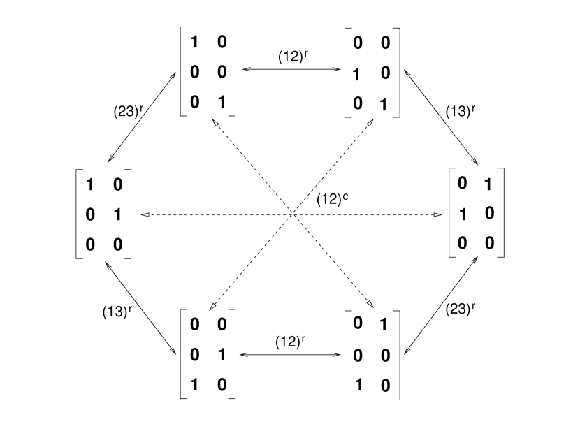
Figure 1: The simplex $\boldsymbol{\Delta^{\star}}$ in case $k=3,d=2$. Connecting edges are shown using unbroken lines and are labelled by the row transposition that interchanges vertices. The simplicies $\boldsymbol{\Delta}(3,2),(12)^{c}\boldsymbol{\Delta}(3,2)$ are both invariant by $\Delta S_{2}$.

The argument is general and applies when $k>d$—that is, when $V\in M(k,d)$ has at least one row of zeros. The connection can always be made through row permutations.

Fossilization of critical points, general case.

The phenomenon described above occurs when the network is over-parameterized. In what follows we assume $V\in M(d,d)$ is a matrix with no zero or parallel rows, and extend in the usual way to $V\in M(k,d)$, $k>d$.

Suppose $W\in M(k,d)$ is a critical point of $\mathcal{L}$: in particular, assume that $\mathcal{L}$ is $C^{2}$ at $W$ and so $W$ has no zero rows. Typically, we assume that $W$ is non-degenerate: all the eigenvalues of the Hessian are non-zero.

Let $\bar{k}>k$ and $\mathfrak{K}^{\star}$ denote the set of all partitions of $[\bar{k}]$ such that each $\mathcal{K}\in\mathfrak{K}^{\star}$ has exactly $k$ parts, $K_{1},\cdots K_{k}$ and $j\in K_{j}$, for all $j\in[k]$.

Just as we did previously, if $\mathcal{K}\in\mathfrak{K}^{\star}$ and $j\in[k]$, we define the simplex $\Delta_{j}(\mathcal{K})\subset{}^{\bar{k}}$, and simplicial set $\Delta(\mathcal{K})=\prod_{j\in[k]}\Delta_{j}(\mathcal{K})\subset M(\bar{k},k)$ of dimension $\bar{k}-k$. Set $\boldsymbol{\Delta}(\bar{k},k)=\cup_{\mathcal{K}\in\mathfrak{K}^{\star}}\Delta(\mathcal{K})$.

Given $W\in M(k,d)$, $\mathcal{K}\in\mathfrak{K}^{\star}$ and $\boldsymbol{\delta}\in\Delta(\mathcal{K})$, define $W_{\delta}\in M(\bar{k},d)$ by

$${\bm{w}}^{\boldsymbol{\delta}}_{i} = \delta_{ii}{\bm{w}}_{i},\;i\in[k]$$

$$= \sum_{j\in[k]}\delta_{ij}{\bm{w}}_{j},\;i>k$$

As we did above when $W=V$, we have $W_{\delta}^{\Sigma}=W^{\Sigma}$. It follows from the definitions that if $\boldsymbol{\delta}\in\Delta(\mathcal{K})$, then $\sum_{\ell\in K_{i}}\boldsymbol{w}_{\ell}^{\boldsymbol{\delta}}={\bm{w}}_{i}$, for all $i\in[k]$.

Given $W\in M(k,d)$, define $\Delta(\bar{k},k)(W)=\{W_{\boldsymbol{\delta}}\mbox{$\;|\;$}\boldsymbol{\delta}\in\Delta(\bar{k},k)\}$ and

$$\boldsymbol{\Delta^{\star}}(W)=\Gamma\Delta(\bar{k},k)(W)\subset M(\bar{k},d).$$

Set $\boldsymbol{\Delta^{\star\star}}(W)=\boldsymbol{\Delta^{\star}}(W)\smallsetminus\partial\boldsymbol{\Delta^{\star}}(W)$

Proposition 1

(Notation and assumptions as above.)

1. $\boldsymbol{\Delta^{\star}}(W)$ is a connected $S_{d}^{r}$-invariant simplical complex of dimension $\bar{k}-k$.

2. $\mathcal{L}$ is $C^{2}$ at all points of ${\boldsymbol{\Delta}}^{\star\star}(W)$ and $\nabla\mathcal{L}|{\boldsymbol{\Delta}}^{\star\star}(W)\equiv 0$

3. $\mathcal{L}$ is constant on $\boldsymbol{\Delta^{\star}}(W)$.

The proof of (1) is similar to that of Theorem 5 (1,2). Since $\boldsymbol{\Delta^{\star}}(W)$ is connected, and $\mathcal{L}$ is continuous, (3) follows from (2) ((3) may be proved directly as in Theorem 5 and then (2) follows using the regularity of $\mathcal{L}$ on ${\boldsymbol{\Delta}}^{\star\star}(W)$). For completeness, we give a direct proof that ${\nabla{\mathcal{L}}}$ vanishes on ${\boldsymbol{\Delta}}^{\star\star}(W)$. By an obvious induction, we can reduce to showing that if the partition $\mathcal{K}\in\mathfrak{K}^{\star}$ satisfies $|K_{i}|=1$, $i<k$ and $|K_{k}|-1=n=\bar{k}-k\geq 1$, then $\nabla\mathcal{L}|\Delta(\mathcal{K})\smallsetminus\partial\Delta(\mathcal{K})\equiv 0$. Set $m=n+1=|K_{k}|$.

By standard results on $\nabla{\mathcal{L}}$ [1], $W$ is a critical point of $\mathcal{L}$ if for $i\in[k]$

$$\sum_{j\in[k]}\left(\frac{\|\boldsymbol{w}_{j}\|\sin(\theta_{\boldsymbol{w}_{i},\boldsymbol{w}_{j}})}{\|\boldsymbol{w}_{i}\|}\boldsymbol{w}_{i}-\theta_{\boldsymbol{w}_{i},\boldsymbol{w}_{j}}\boldsymbol{w}_{j}\right)-\sum_{j\in[d]}\left(\frac{\sin(\theta_{\boldsymbol{w}_{i},\boldsymbol{v}_{j}})}{\|\boldsymbol{w}_{i}\|}\boldsymbol{w}_{i}-\theta_{\boldsymbol{w}_{i},\boldsymbol{v}_{j}}\boldsymbol{v}_{j}\right)+\pi\big{(}W-V\big{)}^{\Sigma}=0$$ (15)

Suppose that $U\in\Delta(\mathcal{K})\smallsetminus\partial\Delta(\mathcal{K})$. In order to check whether or not $U$ is a critical point, $\boldsymbol{w}_{k}$ will be replaced in (15) by $m$ non-zero parallel rows $\boldsymbol{u}_{\ell}=\alpha_{\ell}\boldsymbol{w}_{k}$, where $\sum_{\ell\in[m]}\alpha_{\ell}=1$ and $\alpha_{\ell}>0$, $\ell\in[m]$. Since the new rows $\boldsymbol{u}_{\ell}$ are all non-zero and strictly positive multiples of $\boldsymbol{w}_{k}$,

1. $\theta_{\boldsymbol{w}_{k},\boldsymbol{w}_{j}}=\theta_{\boldsymbol{u}_{\ell},\boldsymbol{w}_{j}},\;j\in[k]$, and $\theta_{\boldsymbol{u}_{\ell},\boldsymbol{u}_{\ell^{\prime}}}=0$ for all $\ell,\ell^{\prime}\in[n]$.

2. $\|\boldsymbol{u}_{\ell}\|=\alpha_{\ell}\|\boldsymbol{w}_{k}\|,\;\ell\in[m]$.

3. $\theta_{\boldsymbol{u}_{\ell},\boldsymbol{v}_{j}}=\theta_{\boldsymbol{w}_{k},\boldsymbol{v}_{j}}$, for all $\ell\in[m]$, $j\in[d]$.

4. $\big{(}W-V\big{)}^{\Sigma}=\big{(}U-V\big{)}^{\Sigma}$ (since $\sum_{\ell\in[m]}\alpha_{\ell}=1$).

We have $m$ new expressions replacing the right hand side of (15) in case $i=k$:

$$\sum_{j\in[\bar{k}]}\left(\frac{\|\boldsymbol{w}_{j}\|\sin(\theta_{\boldsymbol{u}_{\ell},\boldsymbol{w}_{j}})}{\|\boldsymbol{u}_{\ell}\|}\boldsymbol{u}_{\ell}-\theta_{\boldsymbol{u}_{\ell},\boldsymbol{w}_{j}}\boldsymbol{w}_{j}\right)-$$

$$\sum_{j\in[\bar{k}]}\left(\frac{\sin(\theta_{\boldsymbol{u}_{\ell},\boldsymbol{v}_{j}})}{\|\boldsymbol{u}_{\ell}\|}\boldsymbol{u}_{\ell}-\theta_{\boldsymbol{u}_{\ell},\boldsymbol{v}_{j}}\boldsymbol{v}_{j}\right)+\pi\big{(}U-V\big{)}^{\Sigma},$$

where by $\sum_{j\in[\bar{k}]}$, we mean the sum over $\boldsymbol{w}_{j}$ terms, $j\in[k-1]$, and $\boldsymbol{w}_{\ell^{\prime}}$ terms, $\ell^{\prime}\in[m]$. If $\ell\in[m]$, it follows from (A,B) that

$$\sum_{j\in[\bar{k}]}\left(\frac{\|\boldsymbol{w}_{j}\|\sin(\theta_{\boldsymbol{u}_{\ell},\boldsymbol{w}_{j}})}{\|\boldsymbol{u}_{\ell}\|}\boldsymbol{u}_{\ell}-\theta_{\boldsymbol{u}_{\ell},\boldsymbol{w}_{j}}\boldsymbol{w}_{j}\right)=\sum_{j\in[d]}\left(\frac{\|\boldsymbol{w}_{j}\|\sin(\theta_{\boldsymbol{w}_{k},\boldsymbol{w}_{j}})}{\|\boldsymbol{w}_{k}\|}\boldsymbol{w}_{k}-\theta_{\boldsymbol{w}_{\ell},\boldsymbol{w}_{j}}\boldsymbol{w}_{j}\right),$$

and from (B,C) that

$$\sum_{j\in[k]}\left(\frac{\sin(\theta_{\boldsymbol{u}_{\ell},\boldsymbol{v}_{j}})}{\|\boldsymbol{u}_{\ell}\|}\boldsymbol{u}_{\ell}-\theta_{\boldsymbol{u}_{\ell},\boldsymbol{v}_{j}}\boldsymbol{v}_{j}\right)=\sum_{j\in[k]}\left(\frac{\sin(\theta_{\boldsymbol{w}_{k},\boldsymbol{v}_{j}})}{\|\boldsymbol{w}_{i}\|}\boldsymbol{w}_{i}-\theta_{\boldsymbol{w}_{k},\boldsymbol{v}_{j}}\boldsymbol{v}_{j}\right)$$

Noting (D), it follows that $U$ satisfies the critical point equations for $\ell\in[m]$. Along the same lines, but now using the convexity condition $\sum_{\ell\in[m]}\alpha_{\ell}=1$, we verify that $U$ satisfies the critical point equations for $i\in[k-1]$. Hence $U$ is a critical point of $\mathcal{L}$. $\square$

Appendix B Supplementary material for Section 4

We give a brief review of the technique used in this work to compute the Hessian spectrum. The introduction follows [31, 32] verbatim and is provided here for completeness.

Suppose $V\subset{}^{m}$ is a linear subspace, with Euclidean inner product induced from ^m, and $(V,G)$ is an orthogonal $G$-representation.

Lemma 3

[31, Lemma 7, Setion B.1] The representation $(V,G)$ may be written as an orthogonal direct sum $\bigoplus_{i=1}^{m}(\oplus_{j=1}^{p_{i}}V_{ij})$ where $V_{ij}\subset V$, $(V_{ij},G)$ is irreducible, and $(V_{ij},G)$ is isomorphic to $(V_{\ell k},G)$ iff $i=\ell$, and $j,k\in{[p_{i}]}$. The subspaces $\oplus_{j=1}^{p_{i}}V_{ij}$ are unique, $i\in{[m]}$.

If $p_{i}=1$, for all $i\in m$, the orthogonal decomposition given by the lemma is unique, up to order; otherwise the decomposition is not unique. In spite of the lack of uniqueness of Lemma 3, in some cases there may be natural choices of invariant subspace for the irreducible components. This is exactly the situation for the isotypic decomposition of $(M(k,k),G)$, $G=S_{p}\times S_{k-p}$. This naturality allows us to give natural constructions of the matrices $M_{i}$, $i\in{[m]}$, used for determining the spectrum of $G$-maps $A:M(k,k){\rightarrow}M(k,k)$.

The isotypic decomposition for $(M(k,k),S_{k})$ is $2\mathfrak{t}+3\mathfrak{s}+\mathfrak{x}+\mathfrak{y}$, $k\geq 4$ (see Section 4). The subspace of $M(k,k)$ determined by $2\mathfrak{t}$ is the set of all $k\times k$ matrices $\mathcal{T}=\{T_{a,b}\mbox{$\;|\;$}a,b\in\real\}$ where the diagonal entries of $T_{a,b}$ all equal $a$ and the off-diagonal entries all equal $b$. There are many ways to write $\mathcal{T}$ as an orthogonal direct sum. For example, $\mathcal{T}=T_{1,1}\real\oplus T_{\frac{2}{k},-\frac{1}{k(k-1)}}\real$. However, there is only one natural way: $\mathcal{T}=T_{1,0}\real\oplus T_{0,1}\real$. Define $\mathfrak{D}^{k}_{1}=T_{1,0}$, $\mathfrak{D}^{k}_{2}=T_{0,1}$. If we take the standard realization of $(\mathfrak{t},S_{k})$ to be $(\real,S_{k})$, where $S_{k}$ acts trivially on , then we have natural $S_{k}$-maps $\alpha_{1},\alpha_{2}:\real{\rightarrow}M(k,k)$ defined by $\alpha_{i}(t)=t\mathfrak{D}^{k}_{i}$, $i=1,2$. If $A:M(k,k){\rightarrow}M(k,k)$ is an $S_{k}$-map, then $A$ restricts to the $S_{k}$-map $A_{\mathfrak{t}}:\mathcal{T}{\rightarrow}\mathcal{T}$ and $A_{\mathfrak{t}}$ uniquely determines a $2\times 2$-matrix $[a_{ij}]$ by $A_{\mathfrak{t}}(\mathfrak{D}^{k}_{i})=a_{i1}\mathfrak{D}^{k}_{1}+a_{i2}\mathfrak{D}^{k}_{2}$, $i=1,2$. The eigenvalues (and multiplicities in this case) of $A_{\mathfrak{t}}:\mathcal{T}{\rightarrow}\mathcal{T}$ are the same as the eigenvalues of $[a_{ij}]$. If we choose a different orthogonal decomposition of $\mathcal{T}$, we get a different $2\times 2$-matrix that is similar to $[a_{ij}]$ and so has the same eigenvalues. The computation of the rest of the eigenvalues follows similarly.

B.1 Proof of Theorem 3

In Section A.5 algebraic relations between the FPS coefficients are shown to reveal important information on the structure of regular families of critical points. In this section we show how these relations can be further used to evaluate the $\mathfrak{x}$- and the $\mathfrak{y}$-eigenvalues. The method is illustrated for regular families with $b=4$, $k=d+1$ and isotropy $\Delta(S_{d-1}\times S_{1})$.

Referring to notation and results given in Section A.5, any type I or type II family of $\Delta(S_{d-1}\times S_{1})$-critical points must satisfy $c_{0}\in\{\pm 1\}$ and $c_{1}=e_{0}=e_{1}=e_{2}=e_{3}=f_{0}=f_{1}=f_{2}=f_{3}=0$. Below we shall assume that $c_{0}=-1$. The assumption is not needed, and is only introduced for ease of presentation. For non-zero $g_{0}$ and $i_{0}$, the Puiseux series of the eigenvalue associated to the $\mathfrak{x}$-representation is given by:

$$\lambda_{\mathfrak{x}} =-\frac{c_{2}^{2}}{2\pi}-\frac{c_{2}\sqrt{g_{0}^{2}}}{2\pi}-\frac{c_{2}\sqrt{p_{0}^{2}}}{2\pi}+\frac{c_{4}}{2\pi}+\frac{e_{4}^{2}}{4\pi}-\frac{1}{\pi}+\frac{1}{4}+\frac{p_{2}\mbox{sgn}(p_{0})}{2\pi}+\frac{g_{2}\mbox{sgn}(g_{0})}{2\pi}$$ (16)

$$+d^{\frac{1}{4}}\left(\frac{c_{3}}{2\pi}+\frac{p_{1}\mbox{sgn}(p_{0})}{2\pi}+\frac{g_{1}\mbox{sgn}(g_{0})}{2\pi}\right)+d^{\frac{1}{2}}\left(\frac{c_{2}}{2\pi}+\frac{\sqrt{g_{0}^{2}}}{2\pi}+\frac{\sqrt{p_{0}^{2}}}{2\pi}\right)+O(d^{-\frac{1}{4}}).$$

Thus, the expression $\lambda_{\mathfrak{x}}$ depends on FPS coefficients not determined in Section A.5. We show that $\lambda_{\mathfrak{x}}$ can be evaluated nonetheless, independently of the unknown coefficients.

With FPS coefficients as above,

$$[d^{0}]F_{d,1} =\frac{c_{4}}{2\pi}+\frac{e_{4}^{2}}{4\pi}+\frac{e_{4}}{4}+\frac{g_{0}}{4}+\frac{p_{0}}{4}-\frac{1}{2\pi}+\frac{p_{2}\mbox{sgn}(p_{0})}{2\pi}+\frac{g_{2}\mbox{sgn}(g_{0})}{2\pi},$$

$$[d^{\frac{1}{4}}]F_{d,1} =\frac{c_{3}}{2\pi}+\frac{p_{1}\mbox{sgn}(p_{0})}{2\pi}+\frac{g_{1}\mbox{sgn}(g_{0})}{2\pi},$$

$$[d^{\frac{1}{2}}]F_{d,1} =\frac{c_{2}}{2\pi}+\frac{\sqrt{g_{0}^{2}}}{2\pi}+\frac{\sqrt{p_{0}^{2}}}{2\pi},$$ (17)

$$[d^{0}]F_{d,2} =\frac{e_{4}}{4}+\frac{g_{0}}{4}+\frac{p_{0}}{4}.$$

Substituting into (16) gives

$$\lambda_{\mathfrak{x}} =\frac{1}{4}-\frac{1}{2\pi}+[d^{0}]F_{d,1}-c_{2}[d^{\frac{1}{2}}]F_{d,1}-[d^{0}]F_{d,2}+[d^{\frac{1}{4}}]F_{d,1}d^{\frac{1}{4}}+[d^{\frac{1}{2}}]F_{d,1}d^{\frac{1}{2}}+O(d^{-\frac{1}{4}}).$$ (18)

In particular, $\lambda_{\mathfrak{x}}$ can be expressed in terms of $[d^{0}]F_{d,1},[d^{\frac{1}{4}}]F_{d,1},[d^{\frac{1}{2}}]F_{d,1}$ and $[d^{0}]F_{d,2}$. Therefore, by continuity, Equation 18 also applies for $g_{0}=p_{0}=0$. Since gradient entries vanish at critical points, so do their Puiseux coefficients and so $[d^{0}]F_{d,1},[d^{\frac{1}{4}}]F_{d,1},[d^{\frac{1}{2}}]F_{d,1}$ and $[d^{0}]F_{d,2}$ vanish, giving $\lambda_{\mathfrak{x}}=\frac{1}{4}-\frac{1}{2\pi}+O(d^{\frac{1}{4}})$. Equation 18 not only gives the exact value of the $\mathfrak{x}$-eigenvalue to $O(d^{\frac{1}{4}})$-order but also describes its sensitivity to variations in the FPS coefficients. For example, it is seen that varying $c_{2}$ accounts for perturbations of order $O(d^{\frac{1}{2}})$. The derivation of the eigenvalue associated to the $\mathfrak{y}$-representation follows along the same lines, giving

$$\lambda_{\mathfrak{y}} =\frac{1}{4}+\frac{1}{2\pi}+[d^{0}]F_{d,1}-c_{2}[d^{\frac{1}{2}}]F_{d,1}-[d^{0}]F_{d,2}+[d^{\frac{1}{4}}]F_{d,1}d^{\frac{1}{4}}+[d^{\frac{1}{2}}]F_{d,1}d^{\frac{1}{2}}+O(d^{-\frac{1}{4}}).$$ (19)

Similar relations exist between criticality and loss.

References

- [1] Alon Brutzkus and Amir Globerson. Globally optimal gradient descent for a convnet with gaussian inputs. In International conference on machine learning. PMLR, 2017.
- [2] Lenaic Chizat and Francis Bach. On the global convergence of gradient descent for over-parameterized models using optimal transport. Advances in neural information processing systems, 2018.
- [3] Mahdi Soltanolkotabi, Adel Javanmard, and Jason D Lee. Theoretical insights into the optimization landscape of over-parameterized shallow neural networks. IEEE Transactions on Information Theory, 65(2):742–769, 2018.
- [4] Song Mei, Andrea Montanari, and Phan-Minh Nguyen. A mean field view of the landscape of two-layer neural networks. Proceedings of the National Academy of Sciences, 115(33):E7665–E7671, 2018.
- [5] Sebastian Goldt, Madhu S Advani, Andrew M Saxe, Florent Krzakala, and Lenka Zdeborová. Generalisation dynamics of online learning in over-parameterised neural networks. arXiv preprint arXiv:1901.09085, 2019.
- [6] Yuandong Tian. Student specialization in deep rectified networks with finite width and input dimension. In International Conference on Machine Learning. PMLR, 2020.
- [7] Itay M Safran, Gilad Yehudai, and Ohad Shamir. The effects of mild over-parameterization on the optimization landscape of shallow relu neural networks. In Conference on Learning Theory. PMLR, 2021.
- [8] Avrim Blum and Ronald L Rivest. Training a 3-node neural network is np-complete. In Advances in neural information processing systems, pages 494–501, 1989.
- [9] Alon Brutzkus, Amir Globerson, Eran Malach, and Shai Shalev-Shwartz. SGD learns over-parameterized networks that provably generalize on linearly separable data. In 6th International Conference on Learning Representations, ICLR 2018.
- [10] Ohad Shamir. Distribution-specific hardness of learning neural networks. The Journal of Machine Learning Research, 19(1):1135–1163, 2018.
- [11] Simon Du, Jason Lee, Yuandong Tian, Aarti Singh, and Barnabas Poczos. Gradient descent learns one-hidden-layer cnn: Don’t be afraid of spurious local minima. In International Conference on Machine Learning. PMLR, 2018.
- [12] Kai Zhong, Zhao Song, Prateek Jain, Peter L Bartlett, and Inderjit S Dhillon. Recovery guarantees for one-hidden-layer neural networks. In International conference on machine learning. PMLR, 2017.
- [13] Yuanzhi Li and Yang Yuan. Convergence analysis of two-layer neural networks with relu activation. In Advances in Neural Information Processing Systems, pages 597–607, 2017.
- [14] Yuandong Tian. An analytical formula of population gradient for two-layered relu network and its applications in convergence and critical point analysis. In International conference on machine learning. PMLR, 2017.
- [15] Rong Ge, Jason D. Lee, and Tengyu Ma. Learning one-hidden-layer neural networks with landscape design. In 6th International Conference on Learning Representations, ICLR 2018.
- [16] Benjamin Aubin, Antoine Maillard, Jean Barbier, Florent Krzakala, Nicolas Macris, and Lenka Zdeborová. The committee machine: Computational to statistical gaps in learning a two-layers neural network. Journal of Statistical Mechanics: Theory and Experiment, 2019(12):124023, 2019.
- [17] Shunta Akiyama and Taiji Suzuki. On learnability via gradient method for two-layer relu neural networks in teacher-student setting. In International Conference on Machine Learning, pages 152–162. PMLR, 2021.
- [18] Xavier Glorot and Yoshua Bengio. Understanding the difficulty of training deep feedforward neural networks. In Proceedings of the thirteenth international conference on artificial intelligence and statistics, pages 249–256, 2010.
- [19] Itay Safran and Ohad Shamir. Spurious local minima are common in two-layer relu neural networks. In International conference on machine learning. PMLR, 2018.
- [20] Arthur Jacot, Franck Gabriel, and Clément Hongler. Neural tangent kernel: Convergence and generalization in neural networks. Advances in neural information processing systems, 31, 2018.
- [21] Amit Daniely, Roy Frostig, and Yoram Singer. Toward deeper understanding of neural networks: The power of initialization and a dual view on expressivity. Advances in neural information processing systems, 2016.
- [22] Yuanzhi Li, Tengyu Ma, and Hongyang R Zhang. Learning over-parametrized two-layer neural networks beyond ntk. In Conference on learning theory. PMLR, 2020.
- [23] Sebastian Goldt, Madhu Advani, Andrew M Saxe, Florent Krzakala, and Lenka Zdeborová. Dynamics of stochastic gradient descent for two-layer neural networks in the teacher-student setup. Advances in neural information processing systems, 32, 2019.
- [24] Elisa Oostwal, Michiel Straat, and Michael Biehl. Hidden unit specialization in layered neural networks: Relu vs. sigmoidal activation. Physica A: Statistical Mechanics and its Applications, 564:125517, 2021.
- [25] Gilad Yehudai and Ohad Shamir. On the power and limitations of random features for understanding neural networks. Advances in Neural Information Processing Systems, 32, 2019.
- [26] Behrooz Ghorbani, Song Mei, Theodor Misiakiewicz, and Andrea Montanari. When do neural networks outperform kernel methods? Advances in Neural Information Processing Systems, 33, 2020.
- [27] Yossi Arjevani and Michael Field. On the principle of least symmetry breaking in shallow relu models. arXiv preprint arXiv:1912.11939, 2019.
- [28] Yossi Arjevani, Joan Bruna, Michael Field, Joe Kileel, Matthew Trager, and Francis Williams. Symmetry breaking in symmetric tensor decomposition. arXiv preprint arXiv:2103.06234, 2021.
- [29] Yossi Arjevani and Michael Field. Analytic study of spurious minima in symmetric tensor decomposition problems. In preparation.
- [30] Yossi Arjevani and Michael Field. Symmetry & critical points for a model shallow neural network. Physica D: Nonlinear Phenomena, 427:133014, 2021.
- [31] Yossi Arjevani and Michael Field. Analytic characterization of the hessian in shallow relu models: A tale of symmetry. Advances in Neural Information Processing Systems, 33, 2020.
- [32] Yossi Arjevani and Michael Field. Analytic study of families of spurious minima in two-layer relu neural networks: A tale of symmetry ii. Advances in Neural Information Processing Systems, 34, 2021.
- [33] Yossi Arjevani and Michael Field. Equivariant bifurcation, quadratic equivariants, and symmetry breaking for the standard representation of s k. Nonlinearity, 35(6):2809, 2022.
- [34] Roi Livni, Shai Shalev-Shwartz, and Ohad Shamir. On the computational efficiency of training neural networks. Advances in neural information processing systems, 27, 2014.
- [35] Edward Bierstone and Pierre D Milman. Subanalytic geometry. Model theory, algebra, and geometry (ed. by Haskell, D. et al.), MSRI, 39:151–172, 1998.
- [36] John Milnor. Singular points of complex hypersurfaces. Ann. Math. St, 61:591–648, 1968.
- [37] GD James. The representation theory of the symmetric groups. Springer, 1978.
- [38] William Fulton and Joe Harris. Representation theory, volume 129 of. Graduate Texts in Mathematics, 1991.
- [39] Charles R Johnson and Roger A Horn. Matrix analysis. Cambridge university press Cambridge, 1985.
- [40] Saeed Ghadimi and Guanghui Lan. Stochastic first-and zeroth-order methods for nonconvex stochastic programming. SIAM Journal on Optimization, 23(4):2341–2368, 2013.
- [41] Yurii Nesterov and Boris T Polyak. Cubic regularization of newton method and its global performance. Mathematical Programming, 108(1):177–205, 2006.
- [42] Yossi Arjevani, Yair Carmon, John C Duchi, Dylan J Foster, Nathan Srebro, and Blake Woodworth. Lower bounds for non-convex stochastic optimization. Mathematical Programming, pages 1–50, 2022.
- [43] Yossi Arjevani and Michael Field. Bifurcation, spurious minima and over-paramerization. In preparation.
- [44] Suriya Gunasekar, Jason Lee, Daniel Soudry, and Nathan Srebro. Characterizing implicit bias in terms of optimization geometry. In International Conference on Machine Learning, pages 1832–1841. PMLR, 2018.