The Specular Derivative

Abstract

In this paper, we introduce a new generalized derivative, which we term the specular derivative. We establish the Quasi-Rolles’ Theorem, the Quasi-Mean Value Theorem, and the Fundamental Theorem of Calculus in light of the specular derivative. We also investigate various analytic and geometric properties of specular derivatives and apply these properties to several differential equations.

Key words: generalization of derivatives, Fundamental Theorem of Calculus, Quasi-Mean Value Theorem, tangent hyperplanes, differential equations

AMS Subject Classifications: 26A24, 26A27, 26B12, 34A36

1 Introduction

A derivative is a fundamental tool to measure the change of real-valued functions. The application of derivatives has been investigated in diverse fields beyond mathematics. Simultaneously, the generalization of derivatives has been studied in the fields of mathematical analysis, complex analysis, algebra, and geometry. The reason why we investigate to generalize derivatives is that the condition, such as continuity or smoothness or measurability, required to have differentiability is demanding. In this sense, we devote this paper to device a way to generalize a derivative in accordance with our intuition and knowledge.

Let $f$ be a single-variable function defined on an interval $I$ in $\mathbb{R}$ and let $x$ be a point in $I$. In order to avoid confusion we call $f^{\prime}$ a classical derivative in this paper. When we say to generalize a derivative, the precise meaning is to find an operator which a classical derivative implies. Also, generalization of derivatives includes the relationship with Riemann or Lebesgue integration. There is a lot of ways to achieve this task: symmetric derivatives, subderivatives, weak derivatives, Dini derivatives, and so on. Extensive and well-organized survey for the foregoing discussion can be found in [6] and [5]. Subderivatives are motivated the geometric properties of the tangent line with classical derivatives. The concept of subderivatives can be defined in abstract function spaces. Weak derivatives are motivated by the integration by parts formula and is related to the functional analysis. We are interested in the application of generalized derivatives to partial differential equations and refer to Evans [8] and Bressan [4].

In order to refer to our study, we look over symmetric derivatives, denoted by $f^{\ast}$, made by changing the form of the different quotient. Since $f^{\ast}(x)$ dose not depend on the behavior of $f$ at the point $x$, the symmetric derivative $f^{\ast}(x)$ can exist even if $f(x)$ does not exist. Note that the existence of $f^{\ast}(x)$ does not imply the existence of $f^{\prime}(x)$. However, if $f^{\prime}(x)$ exists almost everywhere, then $f^{\ast}(x)$ exists almost everywhere. If $f$ and $f^{\ast}$ are continuous on an open interval $I$, then there exists $x\in I$ such that $f^{\prime}(x)=f^{\ast}(x)$. Symmetric derivatives do not satisfy the classical Rolle’s Theorem and Mean Value Theorem. As replacements so-called the Quasi-Rolle’s Theorem and the Quasi-Mean Value Theorem for continuous functions was proved by Aull [1]. Larson [9] proved that the continuity in Quasi-mean value theorem can be replaced by measurability. As for Quasi-mean value theorem for symmetric derivatives, [11] and [10] can be not only accessible but also extensive. Furthermore, according to Aull [1], the Quasi-Mean Value Theorem implies that symmetric derivatives satisfy the property akin to a Lipschitz condition.

In this paper, we device a new generalized derivative so-called a specular derivative including the classical derivative in not only one-dimensional space $\mathbb{R}$ but also high-dimensional space $\mathbb{R}^{n}$. Also, we examine various analytic and geometric properties of specular derivatives and apply these properties in order to address several differential equations.

To give an intuition, consider a function $f$ which is continuous at $x_{0}$ but not differentiable at $x_{0}$ in $I$ as in Figure 1. Imagine that you shot a light ray from left to right toward a certain mirror and then the light ray makes a turn along at the point $x_{0}$. The light ray can be represented as two lines $\text{T}_{1}$ with the right-hand derivative $f^{\prime}_{+}(x_{0})$ and $\text{T}_{2}$ with the left-hand derivative $f^{\prime}_{-}(x_{0})$ that just touch the function $f$ at the point $x_{0}$. Finally, the mirror must be the line T. Moreover, the angle between $\text{T}_{1}$ and T is equal with the angle between $\text{T}_{2}$ and T. We define the slope of the line T as the specular derivative of $f$ at $x_{0}$, written by $f^{\mathbin{\vbox{\hbox{\scalebox{0.5}{$\bm{\wedge}$}}}}}(x_{0})$. The word “specular” in specular derivatives stands for the mirror T.

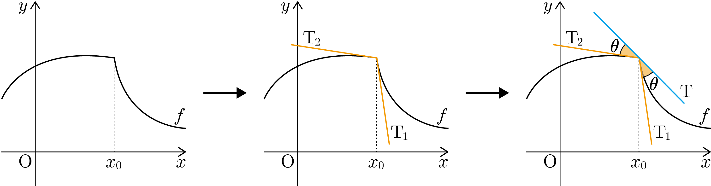
Figure 1: Motivation for specular derivatives

Here are our main results. The specular derivative is well-defined in $\mathbb{R}^{n}$ for each $n\in\mathbb{N}$. In one-dimensional space $\mathbb{R}$, we suggest three ways to calculate a specular derivative and prove that specular derivatives obey Quasi-Rolles’ Theorem and Quasi-Mean Value Theorem. Interestingly, the second order specular differentiability implies the first order classical differentiability. The most noteworthy is the Fundamental Theorem of Calculus can be generalized in the specular derivative sense. By defining a tangent hyperplane in light of specular derivatives, we extend the concepts of specular derivatives in high-dimensional space $\mathbb{R}^{n}$ and provide several examples. Especially, we reveal that the directional derivative with specular derivatives is related to the gradient with specular derivatives and has extrema. As for differential equations, we construct and address the first order ordinary differential equation and the partial differential equation, called the transport equation, with specular derivatives.

The rest of the paper is organized as follows. In Section 2, we define a specular derivative in one-dimensional space $\mathbb{R}$ and state properties of the specular derivative. Section 3 extends the concepts of the specular derivative to high-dimensional space $\mathbb{R}^{n}$. Also, the gradient and directional derivatives for specular derivatives are provided in Section 3. Section 4 deals with differential equations with specular derivatives. Starting from the Fundamental Theorem of Calculus with specular derivatives, Section 4 constructs and solves the first order ordinary differential equation and the transport equation with specular derivatives. Appendix contains delayed proofs, properties useful but elementary, and notations comparing classical derivatives and specular derivatives.

2 Specular derivatives for single-variable functions

Here is our blueprint for specular derivatives in one-dimensional space $\mathbb{R}$. In Figure 2, a function $f$ is specularly differentiable in a open interval $(a,b)\subset\mathbb{R}$ even if $f$ is not defined at a countable sequence $\alpha_{1}$, $\alpha_{2}$, $\cdots$, $\alpha_{n}$ and is not differentiable at some points.

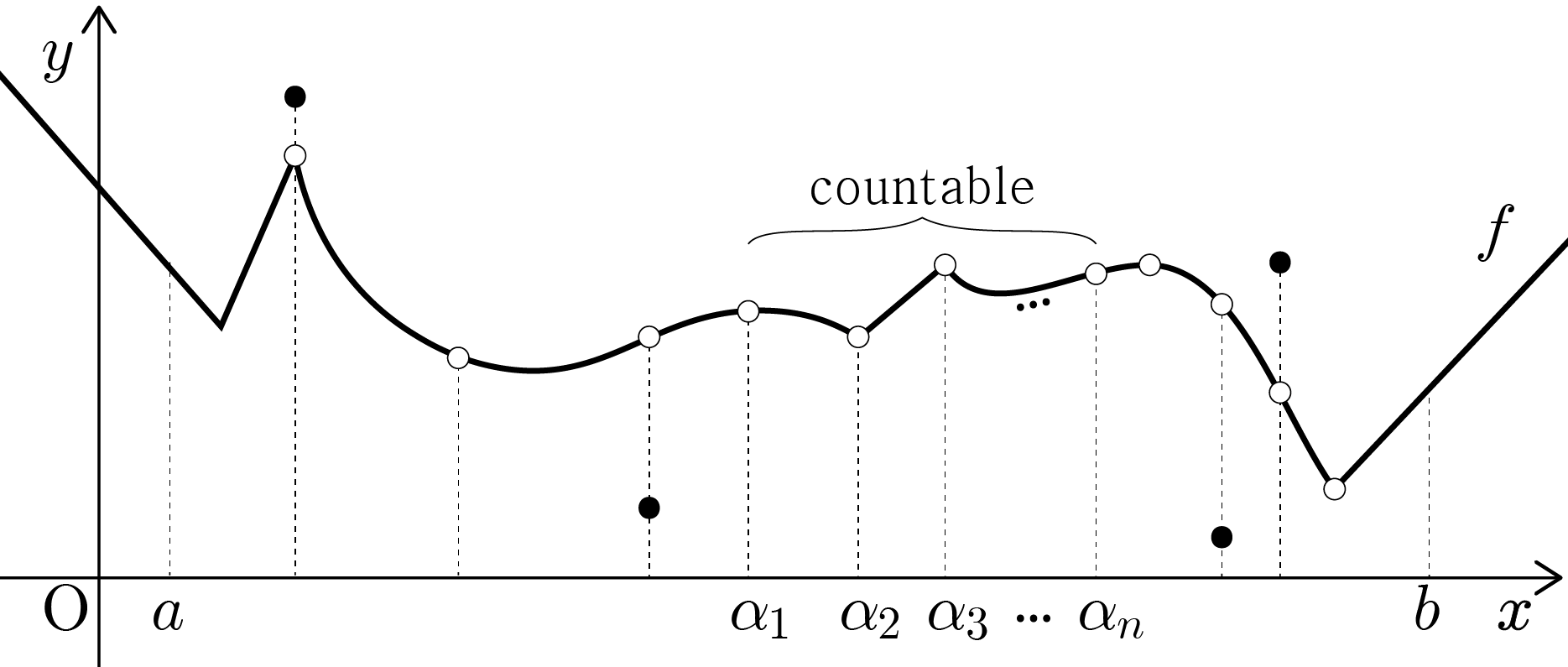
Figure 2: The blueprint for specular derivatives in one-dimension

2.1 Definitions and properties

Definition 2.1.

Let $f:I\to\mathbb{R}$ be a single-variable function with an open interval $I\subset\mathbb{R}$ and $x_{0}$ be a point in $I$. Write

$$f[x_{0}):=\lim_{x\searrow x_{0}}f(x)\qquad\text{and}\qquad f(x_{0}]:=\lim_{x\nearrow x_{0}}f(x)$$

if each limit exists. Also, we denote $f[x_{0}]:=\frac{1}{2}\left(f[x_{0})+f(x_{0}]\right)$.

Definition 2.2.

Let $f:I\to\mathbb{R}$ be a function with an open interval $I\subset\mathbb{R}$ and $x_{0}$ be a point in $I$. We say $f$ is right specularly differentiable at $x_{0}$ if $x_{0}$ is a limit point of $I\cap[x_{0},\infty)$ and the limit

$$f^{\mathbin{\vbox{\hbox{\scalebox{0.5}{$\bm{\wedge}$}}}}}_{+}(x_{0}):=\lim_{x\searrow x_{0}}\frac{f(x)-f[x_{0})}{x-x_{0}}$$

exists as a real number. Similarly, we say $f$ is left specularly differentiable at $x_{0}$ if $x_{0}$ is a limit point of $I\cap(-\infty,x_{0}]$ and the limit

$$f^{\mathbin{\vbox{\hbox{\scalebox{0.5}{$\bm{\wedge}$}}}}}_{-}(x_{0}):=\lim_{x\nearrow x_{0}}\frac{f(x)-f(x_{0}]}{x-x_{0}}$$

exists as a real number. Also, we call $f^{\mathbin{\vbox{\hbox{\scalebox{0.5}{$\bm{\wedge}$}}}}}_{+}(x_{0})$ and $f^{\mathbin{\vbox{\hbox{\scalebox{0.5}{$\bm{\wedge}$}}}}}_{-}(x_{0})$ the (first order) right specular derivative of $f$ at $x_{0}$ and the (first order) left specular derivative of $f$ at $x_{0}$, respectively. In particular, we say $f$ is semi-specularly differentiable at $x_{0}$ if $f$ is right and left specularly differentiable at $x_{0}$.

In Appendix 5.2, we suggest the notation for semi-specular derivatives and employ the notations in this paper.

Remark 2.3.

Clearly, semi-differentiability implies semi-specular differentiability, while the converse does not imply. For example, the sign function is neither right differentiable nor left differentiable at $0$, whereas one can prove that $D^{R}\operatorname{sgn}(0)=0=D^{L}\operatorname{sgn}(0)$.

Definition 2.4.

Let $I$ be an open interval in $\mathbb{R}$ and $x_{0}$ be a point in $I$. Suppose a function $f:I\to\mathbb{R}$ is semi-specularly differentiable at $x_{0}$. We define the phototangent of $f$ at $x_{0}$ to be the function $\operatorname{pht}f:\mathbb{R}\to\mathbb{R}$ by

$$\operatorname{pht}f(y)=\begin{cases}f^{\mathbin{\vbox{\hbox{\scalebox{0.5}{$\bm{\wedge}$}}}}}_{-}(x_{0})(y-x_{0})+f(x_{0}]&\text{if }y<x_{0},\\ f[x_{0}]&\text{if }y=x_{0},\\ f^{\mathbin{\vbox{\hbox{\scalebox{0.5}{$\bm{\wedge}$}}}}}_{+}(x_{0})(y-x_{0})+f[x_{0})&\text{if }y>x_{0}.\end{cases}$$

Definition 2.5.

Let $f:I\to\mathbb{R}$ be a function, where $I$ is a open interval in $\mathbb{R}$. Let $x_{0}$ be a point in $I$. Suppose $f$ is semi-specularly differentiable at $x_{0}$ and let $\operatorname{pht}f$ be the phototangent of $f$ at $x_{0}$. Write $\mathbf{x}_{0}=\left(x_{0},f[x_{0}]\right)\in I\times\mathbb{R}$.

1. The function $f$ is said to be specularly differentiable at $x_{0}$ if $\operatorname{pht}f$ and a circle $\partial B\left(\mathbf{x}_{0},r\right)$ have two intersection points for all $r>0$.

2. Suppose $f$ is specularly differentiable at $x_{0}$ and fix $r>0$. The (first order) specular derivative of $f$ at $x_{0}$, denoted by $f^{\mathbin{\vbox{\hbox{\scalebox{0.5}{$\bm{\wedge}$}}}}}(x_{0})$, is defined to be the slope of the line passing through the two distinct intersection points of $\operatorname{pht}f$ and the circle $\partial B\left(\mathbf{x}_{0},r\right)$.

In particular, if $f$ is specularly differentiable on a closed interval $[a,b]$, then we define specular derivatives at end points: $f^{\mathbin{\vbox{\hbox{\scalebox{0.5}{$\bm{\wedge}$}}}}}(a):=f^{\mathbin{\vbox{\hbox{\scalebox{0.5}{$\bm{\wedge}$}}}}}_{+}(a)$ and $f^{\mathbin{\vbox{\hbox{\scalebox{0.5}{$\bm{\wedge}$}}}}}(b):=f^{\mathbin{\vbox{\hbox{\scalebox{0.5}{$\bm{\wedge}$}}}}}_{-}(b)$. We say $f$ is specularly differentiable on an interval $I$ in $\mathbb{R}$ if $f$ is specularly differentiable at $x_{0}$ for all $x_{0}\in I$.

Note that specular derivatives are translation-invariant. Also, if $f$ is specularly differentiable on an interval $I\subset\mathbb{R}$, then the set of all points at which $f$ has a removable discontinuity is at most countable since $f(x]$ and $f[x)$ exist for all $x\in I$.

Proposition 2.6.

Let $f:I\to\mathbb{R}$ be a function for an open interval $I\subset\mathbb{R}$ and $x_{0}$ be a point in $I$. Suppose there exists a phototangent, say $\operatorname{pht}f$, of $f$ at $x_{0}$. Then $f$ is specularly differentiable at $x_{0}$ if and only if $\operatorname{pht}f$ is continuous at $x_{0}$.

Proof.

Write $\mathbf{x}_{0}=(x_{0},\operatorname{pht}f(x_{0}))$. Let $r>0$ be a real number. Write a circle $\partial B(\mathbf{x}_{0},r)$ as the equation:

$$(x-x_{0})^{2}+(y-\operatorname{pht}f(x_{0}))^{2}=r^{2}$$ (2.1)

for $x,y\in\mathbb{R}$. The system of (2.1) and $\left.\operatorname{pht}f\right|_{[x_{0},\infty)}$ has a root $a$ as well as the system of (2.1) and $\left.\operatorname{pht}f\right|_{(-\infty,x_{0}]}$ has a root $b$:

$$a:=x_{0}+\left(x_{0}^{2}+\frac{r^{2}}{\left(f^{\mathbin{\vbox{\hbox{\scalebox{0.5}{$\bm{\wedge}$}}}}}_{+}(x_{0})\right)^{2}+1}\right)^{\frac{1}{2}}\qquad\text{and}\qquad b:=x_{0}-\left(x_{0}^{2}+\frac{r^{2}}{\left(f^{\mathbin{\vbox{\hbox{\scalebox{0.5}{$\bm{\wedge}$}}}}}_{-}(x_{0})\right)^{2}+1}\right)^{\frac{1}{2}},$$ (2.2)

using the quadratic formula. Notice that $b<a$.

To prove that $\operatorname{pht}f$ is continuous at $x_{0}$, take $\delta:=\min\left\{a-x_{0},x_{0}-b\right\}$. Then $\delta>0$. If $z\in(x_{0}-\delta,x_{0}+\delta)$, then

$$\left|\operatorname{pht}f(x_{0})-\operatorname{pht}f(z)\right|=\left|f[x_{0}]-\operatorname{pht}f(z)\right|\leq\begin{cases}\left|f[x_{0}]-\operatorname{pht}f(b)\right|<r&\text{if }z\in(b,x_{0}],\\ \left|f[x_{0}]-\operatorname{pht}f(a)\right|<r&\text{if }z\in[x_{0},a),\end{cases}$$

which implies that $\operatorname{pht}f$ is continuous at $x_{0}$.

Conversely, the system of (2.1) and $\operatorname{pht}f$ has two distinct roots since $b<x_{0}<a$. Hence, we conclude that $f$ is specularly differentiable at $x_{0}$. ∎

Corollary 2.7.

Let $f$ and $g$ be single valued functions on an open interval $I\subset\mathbb{R}$ containing a point $x_{0}$. Suppose $f$ and $g$ are specularly differentiable at $x_{0}$. Then $f+g$ is specularly differentiable at $x_{0}$ and $\operatorname{pht}f+\operatorname{pht}g=\operatorname{pht}(f+g)$.

Example 2.8.

The phototangent of the sign function at $0$ is itself, which is not continuous at $0$. Hence, the sign function is not specularly differentiable at $0$.

Example 2.9.

The function $f:\mathbb{R}\to\mathbb{R}$ by $f(x)=|x|$ for $x\in\mathbb{R}$ is continuous and specularly differentiable on $\mathbb{R}$. In fact, $f^{\mathbin{\vbox{\hbox{\scalebox{0.5}{$\bm{\wedge}$}}}}}(x)=\operatorname{sgn}(x)$ which is the sign function. Let $g:\mathbb{R}\to\mathbb{R}$ be the function defined by $g(x)=|x|$ if $x\neq 0$ and $g(x)=1$ if $x=0$. Note that $g$ is not continuous at $0$ but is specularly differentiable at $0$ with $g^{\mathbin{\vbox{\hbox{\scalebox{0.5}{$\bm{\wedge}$}}}}}(0)=0$. Consequently, we have $f^{\mathbin{\vbox{\hbox{\scalebox{0.5}{$\bm{\wedge}$}}}}}(x)=g^{\mathbin{\vbox{\hbox{\scalebox{0.5}{$\bm{\wedge}$}}}}}(x)=\operatorname{sgn}(x)$ for all $x\in\mathbb{R}$.

Definition 2.10.

Let $f:I\to\mathbb{R}$ be a function with an interval $I\subset\mathbb{R}$ and a point $x_{0}$ in $I$. Suppose $f$ is specularly differentiable at $x_{0}$. We define the specular tangent line to the graph of $f$ at the point $\left(x_{0},f[x_{0}]\right)$, denoted by $\operatorname{stg}f$, to be the line passing through the point $\left(x_{0},f[x_{0}]\right)$ with slope $f^{\mathbin{\vbox{\hbox{\scalebox{0.5}{$\bm{\wedge}$}}}}}(x_{0})$.

Remark 2.11.

In Definition 2.10, the specular tangent line is given by the function $\operatorname{stg}f:I\to\mathbb{R}$ by

$$\operatorname{stg}f(x)=f^{\mathbin{\vbox{\hbox{\scalebox{0.5}{$\bm{\wedge}$}}}}}(x_{0})(x-x_{0})+f[x_{0}]$$

for $x\in I$. Also, the specular tangent has two properties: $f[x_{0}]=\operatorname{stg}f(x_{0})$ and $f^{\mathbin{\vbox{\hbox{\scalebox{0.5}{$\bm{\wedge}$}}}}}(x_{0})=\left(\operatorname{stg}f\right)^{\mathbin{\vbox{\hbox{\scalebox{0.5}{$\bm{\wedge}$}}}}}(x_{0})$.

In Figure 3, the function $f$ is neither continuous at $x_{0}$ nor differentiable at $x_{0}$. Let $\operatorname{pht}f$ be the phototangent of $f$ at $x_{0}$. We can calculate the specular derivative whenever $\operatorname{pht}f$ is continuous at $x_{0}$. Imagine you shot a light ray toward a mirror. The words “specular” in specular tangent line and “photo” in phototangent stand for the mirror $\operatorname{stg}f$ and the light ray $\operatorname{pht}f$, respectively. Write $\text{C}=\left(x_{0},f[x_{0}]\right)$. Observing that

$$\angle\text{CPQ}=\angle\text{CQP}=\angle\text{SCQ}=\angle\text{TCP},$$

one can find that the slope of the line PQ and the slope of the phototangent of $f$ at $x_{0}$ are equal.

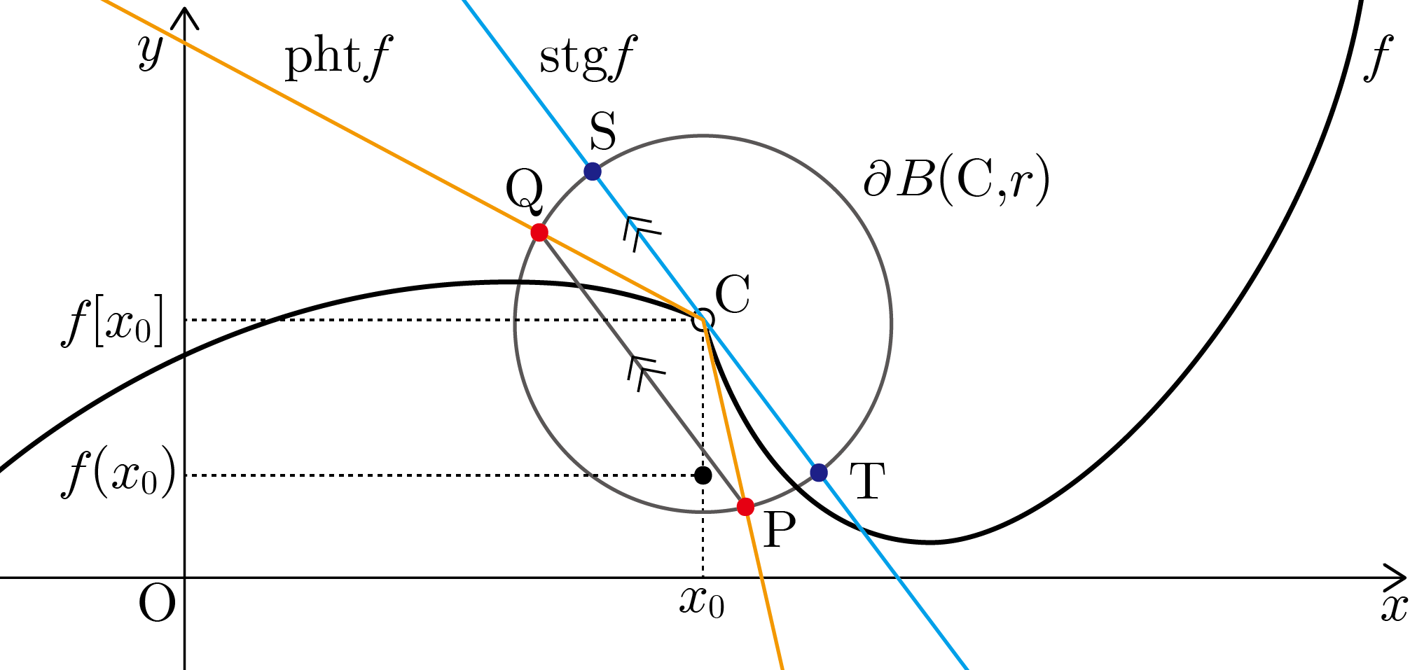
Figure 3: Basic concepts concerning specular derivatives

We suggest three avenues calculating a specular derivative. The first formula can be used as the criterion for the existence of specular derivatives.

Theorem 2.12.

(Specular Derivatives Criterion) Let $f:I\to\mathbb{R}$ be a function with an open interval $I\subset\mathbb{R}$ and $x$ be a point in $I$. If $f$ is specularly differentiable at $x$, then

$$f^{\mathbin{\vbox{\hbox{\scalebox{0.5}{$\bm{\wedge}$}}}}}(x)=\lim_{h\to 0}\frac{\left(f(x+h)-f[x]\right)\sqrt{\left(f(x-h)-f[x]\right)^{2}+h^{2}}-\left(f(x-h)-f[x]\right)\sqrt{\left(f(x+h)-f[x]\right)^{2}+h^{2}}}{h\sqrt{\left(f(x-h)-f[x]\right)^{2}+h^{2}}+h\sqrt{\left(f(x+h)-f[x]\right)^{2}+h^{2}}}.$$

Proof.

Set $\Gamma:=\left\{y-x:y\in I\right\}$ and define the function $g:\Gamma\to\mathbb{R}$ by $g(\gamma)=f(x+\gamma)-f[x]$ for $\gamma\in\Gamma$. Since specular derivatives are translation-invariant, we have $f^{\mathbin{\vbox{\hbox{\scalebox{0.5}{$\bm{\wedge}$}}}}}(x)=g^{\mathbin{\vbox{\hbox{\scalebox{0.5}{$\bm{\wedge}$}}}}}\left(0\right)$. Hence, it suffices to prove that

$$g^{\mathbin{\vbox{\hbox{\scalebox{0.5}{$\bm{\wedge}$}}}}}(0)=\lim_{h\to 0}\frac{g(h)\sqrt{g(-h)^{2}+h^{2}}-g(-h)\sqrt{g(h)^{2}+h^{2}}}{h\sqrt{g(-h)^{2}+h^{2}}+h\sqrt{g(h)^{2}+h^{2}}}.$$

Let $h>0$ be given. Fix $0<r<h$. Since $g$ is specularly differentiable at zero, there exists a circle $\partial B(\text{O},r)$ centered at the origin O with radius $r$. Moreover, the circle $\partial B(0,r)$ has the two distinct points A and B intersecting the half-lines $\overrightarrow{\text{OC}}$ and $\overrightarrow{\text{OD}}$, respectively, where $\text{C}=\left(h,g(h)\right)$ and $\text{D}=\left(-h,g(-h)\right)$. See Figure 4. Observe the similar right triangles:

$$\triangle\text{AFO}\sim\triangle\text{CEO}\qquad\text{and}\qquad\triangle\text{BGO}\sim\triangle\text{DHO},$$

where points $\text{E}=\left(h,0\right)$, $\text{F}=\left(\text{A}\mathbin{\vbox{\hbox{\scalebox{0.5}{$\bullet$}}}}\mathbf{e}_{1},0\right)$, $\text{G}=\left(\text{B}\mathbin{\vbox{\hbox{\scalebox{0.5}{$\bullet$}}}}\mathbf{e}_{1},0\right)$, and $\text{H}=\left(h,0\right)$ with $\mathbf{e}_{1}=\left(1,0\right)$. One can find that

$$\text{F}=\left(\frac{rh}{\sqrt{g(h)^{2}+h^{2}}},0\right)\qquad\text{and}\qquad\text{G}=\left(\frac{-rh}{\sqrt{g(-h)^{2}+h^{2}}},0\right),$$

using basic geometry properties for similar right triangles. Consider the continuous function $q:\mathbb{R}\to\mathbb{R}$ defined by

$$q(z)=\begin{cases}\displaystyle\frac{g(h)}{h}z&\text{if }z<0,\\[5.69046pt] 0&\text{if }z=0,\\ \displaystyle\frac{g(-h)}{h}z&\text{if }z>0,\end{cases}$$

which passes through points D, B, O, A, and C. Using the function $q$, we find that

$$\text{A}=\left(\frac{rh}{\sqrt{g(h)^{2}+h^{2}}},\frac{rg(h)}{\sqrt{g(h)^{2}+h^{2}}}\right)\qquad\text{and}\qquad\text{B}=\left(\frac{-rh}{\sqrt{g(-h)^{2}+h^{2}}},\frac{rg(-h)}{\sqrt{g(-h)^{2}+h^{2}}}\right).$$

Hence, the slope of the line AB is

$$\frac{g(h)\sqrt{g(-h)^{2}+h^{2}}-g(-h)\sqrt{g(h)^{2}+h^{2}}}{h\sqrt{g(-h)^{2}+h^{2}}+h\sqrt{g(h)^{2}+h^{2}}}=:\sigma(h).$$

Note that $\theta_{1}=\angle\text{AOP}$ and $\theta_{2}=\angle\text{BOQ}$ converges to zero as $h\to 0$, where P and Q are the intersection points of the circle $\partial B(\text{O},r)$ and $\operatorname{pht}g$. The definition of the specular derivative yields that $\sigma(h)$ converges to $g^{\mathbin{\vbox{\hbox{\scalebox{0.5}{$\bm{\wedge}$}}}}}(0)$ as $h\searrow 0$. Since the function $\sigma$ is even, we deduce that $\sigma(h)$ converges to $g^{\mathbin{\vbox{\hbox{\scalebox{0.5}{$\bm{\wedge}$}}}}}\left(0\right)$ as $h\to 0$, completing the proof. ∎

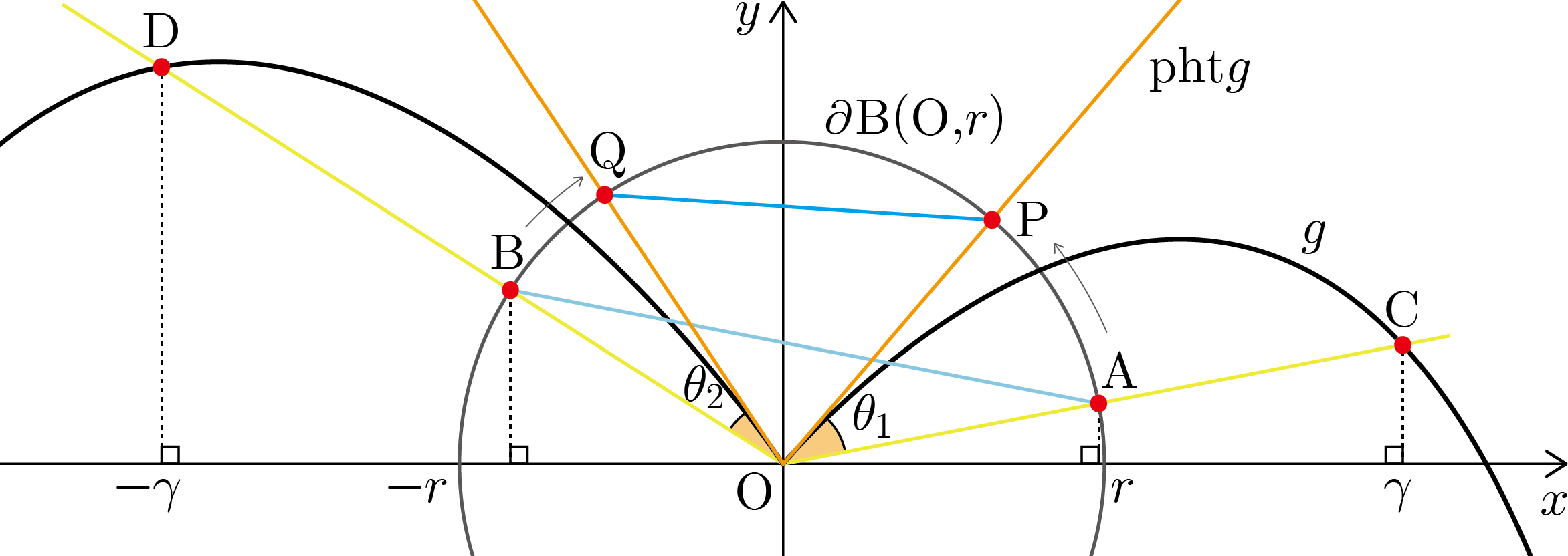
Figure 4: The slope of the line AB converges the specular derivative of $g$ at zero

In the proof of Theorem 2.12, the observation that the function $\sigma$ is even can be generalized as follows:

Corollary 2.13.

Let $f:I\to\mathbb{R}$ be a function with an open interval $I\subset\mathbb{R}$. Let $x_{0}$ be a point in $I$. Assume $f$ is specularly differentiable at $x_{0}$. If $f$ is symmetric about $x=x_{0}$ in a neighborhood of $x_{0}$, that is, there exists $\delta>0$ such that

$$f(x_{0}-x)=f(x_{0}+x)$$

for all $x\in\left(x_{0}-\delta,x_{0}+\delta\right)$. Then $f^{\mathbin{\vbox{\hbox{\scalebox{0.5}{$\bm{\wedge}$}}}}}(x_{0})=0$.

Example 2.14.

For the ReLU function $f(x)=\frac{1}{2}\left(x+|x|\right)$, one can calculate $f^{\mathbin{\vbox{\hbox{\scalebox{0.5}{$\bm{\wedge}$}}}}}(0)=-1+\sqrt{2}$.

In order to calculate specular derivatives more conveniently we suggest the second formula using semi specular derivatives.

Proposition 2.15.

Let $f:I\to\mathbb{R}$ be a function with an open interval $I\subset\mathbb{R}$ and $x_{0}$ be a point in $I$. Assume $f$ is specularly differentiable at $x_{0}$. Write $f^{\mathbin{\vbox{\hbox{\scalebox{0.5}{$\bm{\wedge}$}}}}}_{+}(x_{0})=:\alpha$ and $f^{\mathbin{\vbox{\hbox{\scalebox{0.5}{$\bm{\wedge}$}}}}}_{-}(x_{0})=:\beta$. Then, we have

$$f^{\mathbin{\vbox{\hbox{\scalebox{0.5}{$\bm{\wedge}$}}}}}(x_{0})=\begin{cases}\displaystyle\frac{\alpha\beta-1+\sqrt{\left(\alpha^{2}+1\right)\left(\beta^{2}+1\right)}}{\alpha+\beta}&\text{if }\alpha+\beta\neq 0,\\[12.80365pt] 0&\text{if }\alpha+\beta=0.\end{cases}$$ (2.3)

Proof.

See Appendix 5.1.1. ∎

Since the formula in (2.3) frequently appears on this paper, we state some statements for this formula in Appendix 5.1.2. In fact, the following corollary can be driven directly.

Corollary 2.16.

If $f$ is specularly differentiable at $x_{0}\in\mathbb{R}$, then the following statements hold:

1. $f^{\mathbin{\vbox{\hbox{\scalebox{0.5}{$\bm{\wedge}$}}}}}(x_{0})=0$ if and only if $f^{\mathbin{\vbox{\hbox{\scalebox{0.5}{$\bm{\wedge}$}}}}}_{+}(x_{0})+f^{\mathbin{\vbox{\hbox{\scalebox{0.5}{$\bm{\wedge}$}}}}}_{-}(x_{0})=0$.

2. Signs of $f^{\mathbin{\vbox{\hbox{\scalebox{0.5}{$\bm{\wedge}$}}}}}(x_{0})$ and $f^{\mathbin{\vbox{\hbox{\scalebox{0.5}{$\bm{\wedge}$}}}}}_{+}(x_{0})+f^{\mathbin{\vbox{\hbox{\scalebox{0.5}{$\bm{\wedge}$}}}}}_{-}(x_{0})$ are equal, i.e., $\operatorname{sgn}\left(f^{\mathbin{\vbox{\hbox{\scalebox{0.5}{$\bm{\wedge}$}}}}}(x_{0})\right)=\operatorname{sgn}\left(f^{\mathbin{\vbox{\hbox{\scalebox{0.5}{$\bm{\wedge}$}}}}}_{+}(x_{0})+f^{\mathbin{\vbox{\hbox{\scalebox{0.5}{$\bm{\wedge}$}}}}}_{-}(x_{0})\right)$.

Proof.

The application of Proposition 2.15 and (i), (ii) in Lemma 5.1 with respect to $\alpha=f^{\mathbin{\vbox{\hbox{\scalebox{0.5}{$\bm{\wedge}$}}}}}_{+}(x_{0})$ and $\beta=f^{\mathbin{\vbox{\hbox{\scalebox{0.5}{$\bm{\wedge}$}}}}}_{-}(x_{0})$ completes the proof (see Appendix 5.1.2). ∎

Remark 2.17.

Specular derivatives may do not have linearity. For instance, consider the ReLU function $f(x)=\frac{1}{2}\left(x+|x|\right)$ for $x\in\mathbb{R}$. First, we find that

$$\left(2f\right)^{\mathbin{\vbox{\hbox{\scalebox{0.5}{$\bm{\wedge}$}}}}}(0)=\frac{-1+\sqrt{5}}{2}\neq 2\left(-1+\sqrt{2}\right)=2f^{\mathbin{\vbox{\hbox{\scalebox{0.5}{$\bm{\wedge}$}}}}}(0).$$

Also, take the smooth function $g(x)=2x$ for $x\in\mathbb{R}$. Second, one can calculate that

$$f^{\mathbin{\vbox{\hbox{\scalebox{0.5}{$\bm{\wedge}$}}}}}(0)+g^{\mathbin{\vbox{\hbox{\scalebox{0.5}{$\bm{\wedge}$}}}}}(0)=\left(-1+\sqrt{2}\right)+2\neq\frac{1+\sqrt{5}}{2}=\left.\frac{d}{d^{S}x}\left(\frac{1}{2}\left(5x+\left|x\right|\right)\right)\right|_{x=0}=(f+g)^{\mathbin{\vbox{\hbox{\scalebox{0.5}{$\bm{\wedge}$}}}}}(0).$$

Furthermore, specular derivatives may do not obey the Chain Rule. Consider the composite function $f\circ g:\mathbb{R}\to\mathbb{R}$. Writing $y=g(x)$, we have $x=0$ if and only if $y=0$. Then we find that

$$\left.\frac{df}{d^{S}x}\right|_{x=0}=\frac{-1+\sqrt{5}}{2}\neq\left(-1+\sqrt{2}\right)2=\left.\frac{d}{d^{S}y}\left(\frac{1}{2}\left(y+\left|y\right|\right)\right)\right|_{y=0}\left.\frac{d}{d^{S}x}\left(2x\right)\right|_{x=0}=\left.\frac{df}{d^{S}y}\right|_{y=0}\left.\frac{dy}{d^{S}x}\right|_{x=0}.$$

As stated in the next theorem, the specular derivatives are generalization of classical derivatives.

Theorem 2.18.

Let $f:I\to\mathbb{R}$ be a function with an open interval $I\subset\mathbb{R}$ and a point $x_{0}\in I$.

1. If $f$ is differentiable at $x_{0}$, then $f$ is specularly differentiable at $x_{0}$ and $f^{\prime}(x_{0})=f^{\mathbin{\vbox{\hbox{\scalebox{0.5}{$\bm{\wedge}$}}}}}(x_{0})$.

2. $f$ is differentiable at $x_{0}$ if and only if $f$ is continuous at $x_{0}$ and the phototangent of $f$ at $x_{0}$ is differentiable at $x_{0}$.

Proof.

To prove (i), assume $f$ is differentiable at $x_{0}$. Then $f^{\mathbin{\vbox{\hbox{\scalebox{0.5}{$\bm{\wedge}$}}}}}_{+}(x_{0})=f^{\mathbin{\vbox{\hbox{\scalebox{0.5}{$\bm{\wedge}$}}}}}_{-}(x_{0})<\infty$ and $f$ is continuous at $x_{0}$. It is obvious that the phototangent of $f$ at $x_{0}$ is continuous at $x_{0}$, which implies that $f$ is specularly differentiable at $x_{0}$. If $f^{\mathbin{\vbox{\hbox{\scalebox{0.5}{$\bm{\wedge}$}}}}}_{+}(x_{0})=f^{\mathbin{\vbox{\hbox{\scalebox{0.5}{$\bm{\wedge}$}}}}}_{-}(x_{0})=0$, we see that

$$f^{\prime}(x_{0})=f^{\prime}_{+}(x_{0})=f^{\mathbin{\vbox{\hbox{\scalebox{0.5}{$\bm{\wedge}$}}}}}_{+}(x_{0})=0=f^{\mathbin{\vbox{\hbox{\scalebox{0.5}{$\bm{\wedge}$}}}}}(x_{0}),$$

using Proposition 2.15. On the other hand, if $f^{\mathbin{\vbox{\hbox{\scalebox{0.5}{$\bm{\wedge}$}}}}}_{+}(x_{0})\neq 0$ and $f^{\mathbin{\vbox{\hbox{\scalebox{0.5}{$\bm{\wedge}$}}}}}_{-}(x_{0})\neq 0$, then $f^{\mathbin{\vbox{\hbox{\scalebox{0.5}{$\bm{\wedge}$}}}}}_{+}(x_{0})+f^{\mathbin{\vbox{\hbox{\scalebox{0.5}{$\bm{\wedge}$}}}}}_{-}(x_{0})\neq 0$. Writing $\alpha:=f^{\mathbin{\vbox{\hbox{\scalebox{0.5}{$\bm{\wedge}$}}}}}_{+}(x_{0})$, one can calculate

$$f^{\prime}(x_{0})=f^{\prime}_{+}(x_{0})=f^{\mathbin{\vbox{\hbox{\scalebox{0.5}{$\bm{\wedge}$}}}}}_{+}(x_{0})=\frac{\alpha^{2}-1+\sqrt{\left(\alpha^{2}+1\right)^{2}}}{2\alpha}=f^{\mathbin{\vbox{\hbox{\scalebox{0.5}{$\bm{\wedge}$}}}}}(x_{0})$$

by applying Proposition 2.15 again.

Now, let $\operatorname{pht}f$ be the phototangent of $f$ at $x_{0}$ to show (ii). First, suppose $f$ is differentiable at $x_{0}$. Then $f$ is specularly differentiable at $x_{0}$ by (i). Since $f^{\mathbin{\vbox{\hbox{\scalebox{0.5}{$\bm{\wedge}$}}}}}_{+}(x_{0})=f^{\prime}_{+}(x_{0})=f^{\prime}_{-}(x_{0})=f^{\mathbin{\vbox{\hbox{\scalebox{0.5}{$\bm{\wedge}$}}}}}_{-}(x_{0})$ and $f[x_{0}]=f(x_{0})$, we conclude that $\operatorname{pht}f$ is a polynomial of degree $1$ or less.

Next, write $\operatorname{pht}f$ to indicate the phototangent of $f$ at $x_{0}$. Assume $f$ is continuous at $x_{0}$ and $\operatorname{pht}f$ is differentiable at $x_{0}$. Observing that $\left(\operatorname{pht}f\right)^{\prime}_{+}(x_{0})=\left(\operatorname{pht}f\right)^{\prime}_{-}(x_{0})$, we have $f^{\prime}_{+}(x_{0})=f^{\prime}_{-}(x_{0})$, which implies that $f$ is differentiable at $x_{0}$. ∎

2.2 Application

Specular derivatives does not satisfy neither the classical Roll’s Theorem nor the classical mean value theorem. Take the following function as the counterexample: $f:[-1,1]\to\mathbb{R}$ defined by $f(x)=x+|x|$.

Lemma 2.19.

Let $f$ be a continuous function on $[a,b]\subset\mathbb{R}$. Assume $f$ is specularly differentiable in $(a,b)$. Then the following properties hold:

1. If $f(a)<f(b)$, then there exists $c_{1}\in(a,b)$ such that $f^{\mathbin{\vbox{\hbox{\scalebox{0.5}{$\bm{\wedge}$}}}}}(c_{1})\geq 0$.

2. If $f(a)>f(b)$, then there exists $c_{2}\in(a,b)$ such that $f^{\mathbin{\vbox{\hbox{\scalebox{0.5}{$\bm{\wedge}$}}}}}(c_{2})\leq 0$.

Proof.

First of all, assume $f(a)<f(b)$. Throughout the proof, $k$ denotes a real number with $f(b)<k<f(a)$. Since the set $\left\{x\in[a,b]:f(x)>k\right\}=:K$ is bounded below by $a$, we have $\inf K=:c_{1}$ satisfying $c_{1}\neq a$, $c_{1}\neq b$. Note that $x\in(c_{1}-h,c_{1}+h)$ implies $f(x+h)>k$ and $f(x-h)\leq k$ for small $h>0$. Thanks to the continuity of $f$, we find that

$$f^{\mathbin{\vbox{\hbox{\scalebox{0.5}{$\bm{\wedge}$}}}}}_{+}(c_{1})=f^{\prime}_{+}(c_{1})=\lim_{h\searrow 0}\frac{f(c_{1}+h)-f(c_{1})}{h}\geq\lim_{h\searrow 0}\frac{k-f(c_{1})}{h}=0$$

and

$$f^{\mathbin{\vbox{\hbox{\scalebox{0.5}{$\bm{\wedge}$}}}}}_{-}(c_{1})=f^{\prime}_{-}(c_{1})=\lim_{h\nearrow 0}\frac{f(c_{1}+h)-f(c_{1})}{h}=\lim_{h\searrow 0}\frac{f(c_{1})-f(c_{1}-h)}{h}\geq\lim_{h\searrow 0}\frac{f(c_{1})-k}{h}=0.$$

On the one hand, assume $f^{\mathbin{\vbox{\hbox{\scalebox{0.5}{$\bm{\wedge}$}}}}}_{+}(c_{1})+f^{\mathbin{\vbox{\hbox{\scalebox{0.5}{$\bm{\wedge}$}}}}}_{-}(c_{1})=0$. Then $f^{\mathbin{\vbox{\hbox{\scalebox{0.5}{$\bm{\wedge}$}}}}}(c_{1})=0$ due to Proposition 2.15. On the other hand, suppose $f^{\mathbin{\vbox{\hbox{\scalebox{0.5}{$\bm{\wedge}$}}}}}_{+}(c_{1})+f^{\mathbin{\vbox{\hbox{\scalebox{0.5}{$\bm{\wedge}$}}}}}_{-}(c_{1})\neq 0$. One can estimate that

$$f^{\mathbin{\vbox{\hbox{\scalebox{0.5}{$\bm{\wedge}$}}}}}(c_{1})\geq\frac{f^{\prime}_{+}(c_{1})f^{\prime}_{-}(c_{1})}{f^{\prime}_{+}(c_{1})+f^{\prime}_{-}(c_{1})}\geq 0,$$

using Proposition 2.15. Hence, we conclude that $f^{\mathbin{\vbox{\hbox{\scalebox{0.5}{$\bm{\wedge}$}}}}}(c_{1})\geq 0$.

Similarly, the proof of the reversed inequalities in (ii) can be shown. ∎

Theorem 2.20.

(Quasi-Rolle’s Theorem) Let $f:[a,b]\to\mathbb{R}$ be a continuous function on $[a,b]$. Suppose $f$ is specularly differentiable in $(a,b)$ and $f(a)=f(b)=0$. Then there exist $c_{1}$, $c_{2}\in(a,b)$ such that $f^{\mathbin{\vbox{\hbox{\scalebox{0.5}{$\bm{\wedge}$}}}}}(c_{2})\leq 0\leq f^{\mathbin{\vbox{\hbox{\scalebox{0.5}{$\bm{\wedge}$}}}}}(c_{1})$.

Proof.

If $f\equiv 0$, the conclusion follows. Now, suppose $f\not\equiv 0$. The hypothesis implies three cases; there exists either $a^{\ast}\in(a,b)$ such that $f\left(a^{\ast}\right)>0$, or $b^{\ast}\in(a,b)$ such that $f\left(b^{\ast}\right)<0$, or both. If such $a^{\ast}$ exists, using Lemma 2.19 on $[a,a^{\ast}]$ and $[a^{\ast},b]$ respectively, there exist $c_{1}\in(a,a^{\ast})$ and $c_{2}\in(a^{\ast},b)$ such that $f^{\mathbin{\vbox{\hbox{\scalebox{0.5}{$\bm{\wedge}$}}}}}(c_{2})\leq 0\leq f^{\mathbin{\vbox{\hbox{\scalebox{0.5}{$\bm{\wedge}$}}}}}(c_{1})$. The other remained cases can be shown in a similar way. ∎

In order to prove the Quasi-Mean Value Theorem for specular derivatives, as specular derivatives do not have linearity, we establish a strategy differing from the strategy used in the proof of the classical Mean Value Theorem or Quasi-Mean Value Theorem for symmetric derivatives in [1]. Before that, we suggest the third formula calculating specular derivatives.

Lemma 2.21.

Let $f:I\to\mathbb{R}$ be a function, where $I$ is an open interval in $\mathbb{R}$. Let $x_{0}$ be a point in $I$. Suppose $f$ is specularly differentiable at $x_{0}$. Then

$$\theta=\frac{\theta_{1}+\theta_{2}}{2},$$

where $f^{\mathbin{\vbox{\hbox{\scalebox{0.5}{$\bm{\wedge}$}}}}}_{+}(x_{0})=\tan\theta_{1}$, $f^{\mathbin{\vbox{\hbox{\scalebox{0.5}{$\bm{\wedge}$}}}}}_{-}(x_{0})=\tan\theta_{2}$ and $f^{\mathbin{\vbox{\hbox{\scalebox{0.5}{$\bm{\wedge}$}}}}}(x_{0})=\tan\theta$ for $\theta_{1}$, $\theta_{2}$, $\theta\in\left(-\frac{\pi}{2},\frac{\pi}{2}\right)$.

Proof.

See Appendix 5.1.3. ∎

Theorem 2.22.

(Quasi-Mean Value Theorem) Let $f:[a,b]\to\mathbb{R}$ be a continuous function on $[a,b]\subset\mathbb{R}$. Assume $f$ is specularly differentiable in $(a,b)$. Then there exist points $c_{1}$, $c_{2}\in(a,b)$ such that

$$f^{\mathbin{\vbox{\hbox{\scalebox{0.5}{$\bm{\wedge}$}}}}}(c_{2})\leq\frac{f(b)-f(a)}{b-a}\leq f^{\mathbin{\vbox{\hbox{\scalebox{0.5}{$\bm{\wedge}$}}}}}(c_{1}).$$

Proof.

Write $(f(b)-f(a))/(b-a)=:A$. We consider three cases: $f(a)=f(b)$, $f(a)>f(b)$ and $f(a)<f(b)$. For starters, suppose $f(a)=f(b)$. Let $\phi:[a,b]\to\mathbb{R}$ be a function defined by

$$\phi(x)=f(x)-f(a)$$

for $x\in[a,b]$. Clearly, $\phi$ is continuous on $[a,b]$ and specularly differentiable in $(a,b)$. Observing that $\phi(a)=\phi(b)=0$ and $A=0$, we see that there exist points $c_{1}$, $c_{2}\in[a,b]$ such that $\phi^{\mathbin{\vbox{\hbox{\scalebox{0.5}{$\bm{\wedge}$}}}}}(c_{2})\leq A\leq\phi^{\mathbin{\vbox{\hbox{\scalebox{0.5}{$\bm{\wedge}$}}}}}(c_{1})$ by Theorem 2.20. Since $\phi^{\mathbin{\vbox{\hbox{\scalebox{0.5}{$\bm{\wedge}$}}}}}(x)=f^{\mathbin{\vbox{\hbox{\scalebox{0.5}{$\bm{\wedge}$}}}}}(x)$ for all $x\in[a,b]$, one can deduce that $f^{\mathbin{\vbox{\hbox{\scalebox{0.5}{$\bm{\wedge}$}}}}}(c_{2})\leq A\leq f^{\mathbin{\vbox{\hbox{\scalebox{0.5}{$\bm{\wedge}$}}}}}(c_{1})$.

Next, assume $f(a)<f(b)$. Define the function $\psi:[a,b]\to\mathbb{R}$ by

$$\psi(x)=A(x-a)+f(a)$$

and the set $\Psi:=\left\{x\in[a,b]:f(x)>\psi(x)\right\}$. Then there exist $\inf\Psi=:c_{1}$ and $\sup\Psi=:c_{2}$. First, notice that $f(c_{1}+h)>\psi(c_{1}+h)$, $f(c_{1}-h)\leq\psi(c_{1}-h)$ for small $h>0$ as well as $f(c_{1})\leq\psi(c_{1})$. Write $f^{\mathbin{\vbox{\hbox{\scalebox{0.5}{$\bm{\wedge}$}}}}}_{+}(c_{1})=\tan\theta_{1}$, $f^{\mathbin{\vbox{\hbox{\scalebox{0.5}{$\bm{\wedge}$}}}}}_{-}(c_{1})=\tan\theta_{2}$ and $A=\tan\theta_{0}$, where $\theta_{i}\in\left(-\frac{\pi}{2},\frac{\pi}{2}\right)$ for each $i=0$, $1$, $2$. Observe that

$$\tan\theta_{1}=f^{\mathbin{\vbox{\hbox{\scalebox{0.5}{$\bm{\wedge}$}}}}}_{+}(c_{1})=\lim_{h\searrow 0}\frac{f(c_{1}+h)-f(c_{1})}{h}\geq\lim_{h\searrow 0}\frac{\psi(c_{1}+h)-\psi(c_{1})}{h}=A=\tan\theta_{0}$$

and

$$\tan\theta_{2}=f^{\mathbin{\vbox{\hbox{\scalebox{0.5}{$\bm{\wedge}$}}}}}_{-}(c_{1})=\lim_{h\nearrow 0}\frac{f(c_{1}+h)-f(c_{1})}{h}\geq\lim_{h\nearrow 0}\frac{\psi(c_{1}+h)-\psi(c_{1})}{h}=\lim_{h\searrow 0}\frac{\psi(c_{1})-\psi(c_{1}-h)}{h}=A=\tan\theta_{0},$$

which implies that $\theta_{1}+\theta_{2}\geq 2\theta_{0}$. Writing $f^{\mathbin{\vbox{\hbox{\scalebox{0.5}{$\bm{\wedge}$}}}}}(c_{1})=\tan\theta$ for some $\theta\in\left(-\frac{\pi}{2},\frac{\pi}{2}\right)$, we attain

$$\theta=\frac{\theta_{1}+\theta_{2}}{2}\geq\theta_{0}.$$

Applying Lemma 2.21, we conclude that $f^{\mathbin{\vbox{\hbox{\scalebox{0.5}{$\bm{\wedge}$}}}}}(c_{1})\geq A$. Second, as the same argument is valid with respect to $c_{2}$, one can find that $f^{\mathbin{\vbox{\hbox{\scalebox{0.5}{$\bm{\wedge}$}}}}}(c_{2})\leq A$.

Similarly, the remaining case $f(a)>f(b)$ can be proven. ∎

Even if a continuous function $f$ may not be bounded, $f$ can satisfy the Lipschitz condition provided $f^{\mathbin{\vbox{\hbox{\scalebox{0.5}{$\bm{\wedge}$}}}}}$ is bounded.

Corollary 2.23.

Let $f:(a,b)\to\mathbb{R}$ be a continuous function on $(a,b)$. Assume $f^{\mathbin{\vbox{\hbox{\scalebox{0.5}{$\bm{\wedge}$}}}}}$ is bounded on $(a,b)$. Let $x_{1}$, $x_{2}$ be points in $(a,b)$. Then there exists a constant $M>0$ such that

$$\left|f(x_{1})-f(x_{2})\right|\leq M|x_{1}-x_{2}|,$$

where $M$ is independent of $x_{1}$ and $x_{2}$.

Proof.

Since $f^{\mathbin{\vbox{\hbox{\scalebox{0.5}{$\bm{\wedge}$}}}}}$ is bounded, $\left|f^{\mathbin{\vbox{\hbox{\scalebox{0.5}{$\bm{\wedge}$}}}}}(x)\right|\leq M$ for some constant $M>0$ for any $x\in(a,b)$. By Theorem 2.22, we have

$$-M\leq\frac{f(x_{1})-f(x_{2})}{x_{1}-x_{2}}\leq M$$

for any points $x_{1}$, $x_{2}\in(a,b)$, as required. ∎

Applying the Quasi-Mean Value Theorem for specular derivatives, one can find that the continuity of $f^{\mathbin{\vbox{\hbox{\scalebox{0.5}{$\bm{\wedge}$}}}}}$ at a point $x_{0}$ and the continuity of $f$ on a neighborhood of the point $x_{0}$ entail the existence of $f^{\prime}(x_{0})$. To achieve this, we first suggest the weaker proposition as follows.

Proposition 2.24.

Let $f:(a,b)\to\mathbb{R}$ be a function. Assume $f$ is specularly differentiable in $(a,b)$. Suppose $f$ and $f^{\mathbin{\vbox{\hbox{\scalebox{0.5}{$\bm{\wedge}$}}}}}$ is continuous on $(a,b)$. Then for each point $x\in(a,b)$ there exists $f^{\prime}(x)$ and $f^{\prime}(x)=f^{\mathbin{\vbox{\hbox{\scalebox{0.5}{$\bm{\wedge}$}}}}}(x)$.

Proof.

Let $x$ be a point in $(a,b)$. Choose $h>0$ to be sufficiently small so that $(x-h,x+h)\subset(a,b)$. Applying Theorem 2.22 to $f$ on $[x,x+h]$, there exist points $c_{1}$, $c_{2}$ in $(x,x+h)$ such that

$$f^{\mathbin{\vbox{\hbox{\scalebox{0.5}{$\bm{\wedge}$}}}}}(c_{2})\leq\frac{f(x+h)-f(x)}{h}\leq f^{\mathbin{\vbox{\hbox{\scalebox{0.5}{$\bm{\wedge}$}}}}}(c_{1}).$$

Thanks to the Intermediate Value Theorem for the continuous function $f^{\mathbin{\vbox{\hbox{\scalebox{0.5}{$\bm{\wedge}$}}}}}$, there exists a point $c_{3}\in(x,x+h)$ such that

$$f^{\mathbin{\vbox{\hbox{\scalebox{0.5}{$\bm{\wedge}$}}}}}(c_{3})=\frac{f(x+h)-f(x)}{h}.$$

Taking the limit of both sides as $h\to 0$, we see that

$$f^{\mathbin{\vbox{\hbox{\scalebox{0.5}{$\bm{\wedge}$}}}}}(x)=\lim_{h\to 0}f^{\mathbin{\vbox{\hbox{\scalebox{0.5}{$\bm{\wedge}$}}}}}(c_{3})=\lim_{h\to 0}\frac{f(x+h)-f(x)}{h}=f^{\prime}(x),$$

as required. ∎

Here we state the stronger theorem compared to the above proposition.

Theorem 2.25.

Let $x_{0}$ be a point in $\mathbb{R}$. Let $f:\mathbb{R}\to\mathbb{R}$ be a function to be specularly differentiable at $x_{0}$. Suppose $f$ is continuous in a neighborhood of $x_{0}$ and $f^{\mathbin{\vbox{\hbox{\scalebox{0.5}{$\bm{\wedge}$}}}}}$ is continuous at $x_{0}$. Then $f^{\prime}(x_{0})$ exists and $f^{\prime}(x_{0})=f^{\mathbin{\vbox{\hbox{\scalebox{0.5}{$\bm{\wedge}$}}}}}(x_{0})$.

Proof.

Let $\varepsilon>0$ be given. Using the continuity of $f^{\mathbin{\vbox{\hbox{\scalebox{0.5}{$\bm{\wedge}$}}}}}$ at $x_{0}$, choose $B_{\delta}(x_{0})$ to be a neighborhood of $x_{0}$ with $\delta>0$ such that $f$ is continuous at $x$ and

$$f^{\mathbin{\vbox{\hbox{\scalebox{0.5}{$\bm{\wedge}$}}}}}(x_{0})-\varepsilon<f^{\mathbin{\vbox{\hbox{\scalebox{0.5}{$\bm{\wedge}$}}}}}(x)<f^{\mathbin{\vbox{\hbox{\scalebox{0.5}{$\bm{\wedge}$}}}}}(x_{0})+\varepsilon$$ (2.4)

whenever a point $x\in B_{\delta}(x_{0})$. Choose $h>0$ to be sufficiently small so that $(x_{0}-h,x_{0}+h)\subset B_{\delta}(x_{0})$. Owing to Theorem 2.22 to $f$ on $[x_{0},x_{0}+h]$, there exist points $c_{1}$, $c_{2}$ in $(x_{0},x_{0}+h)$ such that

$$f^{\mathbin{\vbox{\hbox{\scalebox{0.5}{$\bm{\wedge}$}}}}}(c_{2})\leq\frac{f(x_{0}+h)-f(x_{0})}{h}\leq f^{\mathbin{\vbox{\hbox{\scalebox{0.5}{$\bm{\wedge}$}}}}}(c_{1}).$$

Since $c_{1}$ and $c_{2}$ are in $B_{\delta}(x_{0})$, we finally obtain that

$$f^{\mathbin{\vbox{\hbox{\scalebox{0.5}{$\bm{\wedge}$}}}}}(x_{0})-\varepsilon<\frac{f(x_{0}+h)-f(x_{0})}{h}<f^{\mathbin{\vbox{\hbox{\scalebox{0.5}{$\bm{\wedge}$}}}}}(x_{0})+\varepsilon$$

from (2.4), as required. ∎

2.3 Higher order specular derivatives

Naturally, one can try to extend an order of specular derivatives as classical derivatives. Let $f:I\to\mathbb{R}$ be a function, where $I\subset\mathbb{R}$ is an open interval containing a point $x_{0}$. Writing $f^{[1]}:=f^{\mathbin{\vbox{\hbox{\scalebox{0.5}{$\bm{\wedge}$}}}}}$, for each positive integer $n\geq 2$, we recursively define the $n$-th order specularly derivative of $f$ at $x_{0}$ as

$$f^{[n]}(x_{0}):=\left(f^{[n-1]}\right)^{\mathbin{\vbox{\hbox{\scalebox{0.5}{$\bm{\wedge}$}}}}}(x_{0})$$

if these specular derivatives exist. Also, we suggest the notation of higher order specularly derivatives in Appendix 5.2. Especially, we write the second order specularly derivative of $f$ at $x_{0}$ by

$$f^{\mathbin{\vbox{\hbox{\scalebox{0.5}{$\bm{\wedge}$}}}}\mathbin{\vbox{\hbox{\scalebox{0.5}{$\bm{\wedge}$}}}}}(x_{0}):=\left(f^{\mathbin{\vbox{\hbox{\scalebox{0.5}{$\bm{\wedge}$}}}}}\right)^{\mathbin{\vbox{\hbox{\scalebox{0.5}{$\bm{\wedge}$}}}}}(x_{0}).$$

The bottom line is that the second order specularly differentiability of a continuous function implies the classical differentiability.

Proposition 2.26.

Let $f:I\to\mathbb{R}$ be a function with an open interval $I\subset\mathbb{R}$. If $f$ is continuous on $I$ and there exists $f^{\mathbin{\vbox{\hbox{\scalebox{0.5}{$\bm{\wedge}$}}}}\mathbin{\vbox{\hbox{\scalebox{0.5}{$\bm{\wedge}$}}}}}(x)$ for all $x\in I$, then $f^{\mathbin{\vbox{\hbox{\scalebox{0.5}{$\bm{\wedge}$}}}}}$ is continuous on $I$.

Proof.

Let $x_{0}$ be a point in $I$. We claim that $f^{\mathbin{\vbox{\hbox{\scalebox{0.5}{$\bm{\wedge}$}}}}}$ is continuous at $x_{0}$. Let $\displaystyle\lim_{x\to x_{0}}f^{\mathbin{\vbox{\hbox{\scalebox{0.5}{$\bm{\wedge}$}}}}}(x)=:\alpha$. Let $\varepsilon>0$ be given. Then there exists $\delta>0$ such that

$$\left|f^{\mathbin{\vbox{\hbox{\scalebox{0.5}{$\bm{\wedge}$}}}}}(x)-\alpha\right|<\varepsilon$$ (2.5)

whenever $0<\left|x-x_{0}\right|<\delta$. From Lemma 2.21, we know that either

$$f^{\mathbin{\vbox{\hbox{\scalebox{0.5}{$\bm{\wedge}$}}}}}_{-}(x_{0})\leq f^{\mathbin{\vbox{\hbox{\scalebox{0.5}{$\bm{\wedge}$}}}}}(x_{0})\leq f^{\mathbin{\vbox{\hbox{\scalebox{0.5}{$\bm{\wedge}$}}}}}_{+}(x_{0})\qquad\text{or}\qquad f^{\mathbin{\vbox{\hbox{\scalebox{0.5}{$\bm{\wedge}$}}}}}_{+}(x_{0})\leq f^{\mathbin{\vbox{\hbox{\scalebox{0.5}{$\bm{\wedge}$}}}}}(x_{0})\leq f^{\mathbin{\vbox{\hbox{\scalebox{0.5}{$\bm{\wedge}$}}}}}_{-}(x_{0}),$$

using the fact that the tangent function is increasing. Without loss of generality, assume

$$f^{\mathbin{\vbox{\hbox{\scalebox{0.5}{$\bm{\wedge}$}}}}}_{-}(x_{0})\leq f^{\mathbin{\vbox{\hbox{\scalebox{0.5}{$\bm{\wedge}$}}}}}(x_{0})\leq f^{\mathbin{\vbox{\hbox{\scalebox{0.5}{$\bm{\wedge}$}}}}}_{+}(x_{0}).$$ (2.6)

Each definition of $f^{\mathbin{\vbox{\hbox{\scalebox{0.5}{$\bm{\wedge}$}}}}}_{+}(x_{0})$ and $f^{\mathbin{\vbox{\hbox{\scalebox{0.5}{$\bm{\wedge}$}}}}}_{-}(x_{0})$ implies

$$f^{\mathbin{\vbox{\hbox{\scalebox{0.5}{$\bm{\wedge}$}}}}}_{+}(x_{0})\leq\frac{f(x_{1})-f(x_{0})}{x_{1}-x_{0}}+\varepsilon\qquad\text{and}\qquad\frac{f(x_{2})-f(x_{0})}{x_{2}-x_{0}}-\varepsilon\leq f^{\mathbin{\vbox{\hbox{\scalebox{0.5}{$\bm{\wedge}$}}}}}_{-}(x_{0})$$ (2.7)

for some $x_{1}\in(x_{0},x_{0}+\delta)$ and $x_{2}\in\left(x_{0}-\delta,x_{0}\right)$, respectively. Applying twice Theorem 2.22 to $f$ on $\left[x_{0},x_{1}\right]$ and $\left[x_{2},x_{0}\right]$, there exist $x_{1}^{\ast}\in\left(x_{0},x_{1}\right)$ and $x_{2}^{\ast}\in\left(x_{2},x_{0}\right)$ such that

$$\frac{f(x_{1})-f(x_{0})}{x_{1}-x_{0}}\leq f^{\mathbin{\vbox{\hbox{\scalebox{0.5}{$\bm{\wedge}$}}}}}(x_{1}^{\ast})\qquad\text{and}\qquad f^{\mathbin{\vbox{\hbox{\scalebox{0.5}{$\bm{\wedge}$}}}}}(x_{2}^{\ast})\leq\frac{f(x_{2})-f(x_{0})}{x_{2}-x_{0}}.$$ (2.8)

Combining inequalities in (2.6), (2.7), and (2.8), we obtain

$$f^{\mathbin{\vbox{\hbox{\scalebox{0.5}{$\bm{\wedge}$}}}}}(x_{2}^{\ast})-\varepsilon\leq f^{\mathbin{\vbox{\hbox{\scalebox{0.5}{$\bm{\wedge}$}}}}}(x_{0})\leq f^{\mathbin{\vbox{\hbox{\scalebox{0.5}{$\bm{\wedge}$}}}}}(x_{1}^{\ast})+\varepsilon.$$ (2.9)

Since $x_{0}-\delta<x_{2}^{\ast}<x_{0}<x_{1}^{\ast}<x_{0}+\delta$, we find that

$$f^{\mathbin{\vbox{\hbox{\scalebox{0.5}{$\bm{\wedge}$}}}}}(x_{1}^{\ast})<\alpha+\varepsilon\qquad\text{and}\qquad\alpha-\varepsilon<f^{\mathbin{\vbox{\hbox{\scalebox{0.5}{$\bm{\wedge}$}}}}}(x_{2}^{\ast})$$

from (2.5). Combining with (2.9) yields that

$$\alpha-2\varepsilon<f^{\mathbin{\vbox{\hbox{\scalebox{0.5}{$\bm{\wedge}$}}}}}(x_{0})<\alpha+2\varepsilon.$$

Since $\varepsilon>0$ was arbitrary, we have

$$f^{\mathbin{\vbox{\hbox{\scalebox{0.5}{$\bm{\wedge}$}}}}}(x_{0})=\alpha=\lim_{x\to x_{0}}f^{\mathbin{\vbox{\hbox{\scalebox{0.5}{$\bm{\wedge}$}}}}}(x).$$

Consequently, we conclude that $f^{\mathbin{\vbox{\hbox{\scalebox{0.5}{$\bm{\wedge}$}}}}}$ is continuous at $x_{0}$. ∎

Theorem 2.27.

Let $f:I\to\mathbb{R}$ be a function with an open interval $I\subset\mathbb{R}$. Suppose $f$ is continuous on $I$ and there exists $f^{\mathbin{\vbox{\hbox{\scalebox{0.5}{$\bm{\wedge}$}}}}\mathbin{\vbox{\hbox{\scalebox{0.5}{$\bm{\wedge}$}}}}}(x)$ for all $x\in I$. Then there exists $f^{\prime}(x)$ and $f^{\prime}(x)=f^{\mathbin{\vbox{\hbox{\scalebox{0.5}{$\bm{\wedge}$}}}}}(x)$ whenever $x\in I$.

Proof.

Proposition 2.24 and Proposition 2.26 yield the conclusion of this theorem. ∎

Instead, what we are interested in is how to define specular derivatives in high-dimensions and their properties. We discuss this topic in the next section.

3 Specular derivatives for multi-variable functions

In stating specular derivatives and their properties in high-dimensional space $\mathbb{R}^{n}$, we mainly refer to [7].

3.1 Definitions and properties

Definition 3.1.

Let $f:U\to\mathbb{R}$ be a multi-variable function with an open set $U\subset\mathbb{R}^{n}$. Let $\mathbf{x}=(x_{1},x_{2},\cdots,x_{n})$ denote a point of $\mathbb{R}^{n}$. Let $\mathbf{a}=(a_{1},a_{2},\cdots,a_{n})$ be a point in $U$. For $1\leq i\leq n$, we define

$$f[\mathbf{a})_{(i)}:=f[a_{1},a_{2},\cdots,a_{n})_{(i)}:=\lim_{h\searrow 0}f(\mathbf{a}+h\mathbf{e}_{i})\qquad\text{and}\qquad f(\mathbf{a}]_{(i)}:=f(a_{1},a_{2},\cdots,a_{n}]_{(i)}:=\lim_{h\nearrow 0}f(\mathbf{a}+h\mathbf{e}_{i})$$

if each limit exists, where $\mathbf{e}_{i}$ is the $i$-th standard basis vector of $\mathbb{R}^{n}$. Also we denote $f[\mathbf{a}]_{(i)}:=\frac{1}{2}\left(f[\mathbf{a})_{(i)}+f(\mathbf{a}]_{(i)}\right)$ and

$$\overline{\mathbf{a}}_{(i)}:=\left(\mathbf{a},f[\mathbf{a}]_{(i)}\right):=\left(a_{1},a_{2},\cdots,a_{n},f[\mathbf{a}]_{(i)}\right),$$

where $1\leq i\leq n$. In particular, if $f[\mathbf{a}]_{(1)}=f[\mathbf{a}]_{(2)}=\cdots=f[\mathbf{a}]_{(n)}$, we write the common value as $f[\mathbf{a}]$.

Definition 3.2.

Let $U$ be an open subset of $\mathbb{R}^{n}$ and $f:U\rightarrow\mathbb{R}$ be a function. Let $\mathbf{x}=(x_{1},x_{2},\cdots,x_{n})$ denote a point of $\mathbb{R}^{n}$. Let $\mathbf{a}=\left(a_{1},a_{2},\cdots,a_{n}\right)$ be a point in $U$. For $1\leq i\leq n$, we define the (first order) right specularly partial derivative of $f$ at $\mathbf{a}$ with respect to the variable $x_{i}$ to be the limit

$$\partial^{R}_{x_{i}}f(\mathbf{a}):=\lim_{h\searrow 0}\frac{f(\mathbf{a}+h\mathbf{e}_{i})-f[\mathbf{a})_{(i)}}{h}$$

as a real number. Similarly, we say $f$ is the (first order) left specularly partial derivative of $f$ at $\mathbf{a}$ with respect to the variable $x_{i}$ to be the limit

$$\partial^{L}_{x_{i}}f(\mathbf{a}):=\lim_{h\nearrow 0}\frac{f(\mathbf{a}+h\mathbf{e}_{i})-f(\mathbf{a}]_{(i)}}{h}$$

as a real number. Especially, we say $f$ is (first order) semi-specularly partial differentiable at $\mathbf{a}$ with respect to the variable $x_{i}$ if there exist both $\partial^{R}_{x_{i}}f(\mathbf{a})$ and $\partial^{L}_{x_{i}}f(\mathbf{a})$.

We suggest the notation of semi-specularly partial derivatives in Appendix 5.2. Furthermore, consider one-dimension $\mathbb{R}$ together with abused notation $\partial^{R}_{x}f(\mathbf{a})=f^{\mathbin{\vbox{\hbox{\scalebox{0.5}{$\bm{\wedge}$}}}}}_{+}(a)$ and $\partial^{L}_{x}f(\mathbf{a})=f^{\mathbin{\vbox{\hbox{\scalebox{0.5}{$\bm{\wedge}$}}}}}_{-}(a)$ where $\mathbf{a}:=\left(a\right):=a\in\mathbb{R}$. In this context, Definition 3.1 and 3.2 make sense in extending semi-specular derivatives from one-dimension to high-dimensions.

Example 3.3.

Consider the function $f:\mathbb{R}^{2}\to\mathbb{R}$ defined by

$$f(x,y)=\begin{cases}\left|x+y\right|&\text{if }x+y\neq 0,\\ -1&\text{if }x+y=0,\end{cases}$$

for $(x,y)\in\mathbb{R}^{2}$. Define the set $W:=\left\{\left(w_{1},w_{2}\right)\in\mathbb{R}^{2}:w_{1}+w_{2}=0\right\}$. Let $\mathbf{w}=(w_{1},w_{2})$ be a point in $W$. Writing $x=x_{1}$ and $y=x_{2}$, one can compute

$$f[\mathbf{w})_{(1)}=\lim_{h\searrow 0}|w_{1}+h+w_{2}|=0=\lim_{h\nearrow 0}|w_{1}+h+w_{2}|=f(\mathbf{w}]_{(1)}$$

so that

$$\partial^{R}_{x}f(\mathbf{w})=\lim_{h\searrow 0}\frac{f(w_{1}+h,w_{2})-f[w_{1},w_{2})_{(1)}}{h}=\lim_{h\searrow 0}\frac{|w_{1}+h+w_{2}|}{h}=\lim_{h\nearrow 0}\frac{|h|}{h}=1$$

and

$$\partial^{L}_{x}f(\mathbf{w})=\lim_{h\nearrow 0}\frac{f(w_{1}+h,w_{2})-f[w_{1},w_{2})_{(1)}}{h}=\lim_{h\nearrow 0}\frac{|w_{1}+h+w_{2}|}{h}=\lim_{h\nearrow 0}\frac{|h|}{h}=-1.$$

To define specular derivatives in high-dimensions, it needs to define phototangents in high-dimensions first. We naturally define the $n$-dimensional version of phototangents to enable one to still apply the properties of specular derivatives in one-dimension.

Definition 3.4.

Suppose that $U$ is an open subset of $\mathbb{R}^{n}$ and $f:U\rightarrow\mathbb{R}$ is a function. Let $\mathbf{x}=(x_{1},x_{2},\cdots,x_{n})$ denote a point of $\mathbb{R}^{n}$ and let $\mathbf{a}=\left(a_{1},a_{2},\cdots,a_{n}\right)$ be a point in $U$. For $1\leq i\leq n$, write $\mathbf{e}_{i}$ for the $i$-th standard basis vector of $\mathbb{R}^{n}$.

1. For $1\leq i\leq n$, we define the section of the domain $U$ of the function $f$ by the point $\mathbf{a}$ with respect to the variable $x_{i}$ to be the set

   $$U_{x_{i}}(\mathbf{a}):=\left\{\mathbf{x}\in U:\mathbf{x}\mathbin{\vbox{\hbox{\scalebox{0.5}{$\bullet$}}}}\mathbf{e}_{j}=\mathbf{a}\mathbin{\vbox{\hbox{\scalebox{0.5}{$\bullet$}}}}\mathbf{e}_{j}\text{ for all }1\leq j\leq n\text{ with }j\neq i\right\}.$$

2. For $1\leq i\leq n$, assume $f$ is semi-specularly partial differentiable at $\mathbf{a}$ with respect to the variable $x_{i}$. We define a phototangent of $f$ at $\mathbf{a}$ with respect to the variable $x_{i}$ to be the function $\operatorname{pht}_{x_{i}}f:\mathbb{R}^{n}_{x_{i}}(\mathbf{a})\to\mathbb{R}$ defined by

   $$\operatorname{pht}_{x_{i}}f(\mathbf{y})=\begin{cases}\partial^{L}_{x_{i}}f(\mathbf{a})\left(\mathbf{y}\mathbin{\vbox{\hbox{\scalebox{0.5}{$\bullet$}}}}\mathbf{e}_{i}-\mathbf{a}\mathbin{\vbox{\hbox{\scalebox{0.5}{$\bullet$}}}}\mathbf{e}_{i}\right)+f(\mathbf{a}]_{(i)}&\text{if }\mathbf{y}\mathbin{\vbox{\hbox{\scalebox{0.5}{$\bullet$}}}}\mathbf{e}_{i}<\mathbf{a}\mathbin{\vbox{\hbox{\scalebox{0.5}{$\bullet$}}}}\mathbf{e}_{i},\\ f[\mathbf{a}]_{(i)}&\text{if }\mathbf{y}\mathbin{\vbox{\hbox{\scalebox{0.5}{$\bullet$}}}}\mathbf{e}_{i}=\mathbf{a}\mathbin{\vbox{\hbox{\scalebox{0.5}{$\bullet$}}}}\mathbf{e}_{i},\\ \partial^{R}_{x_{i}}f(\mathbf{a})\left(\mathbf{y}\mathbin{\vbox{\hbox{\scalebox{0.5}{$\bullet$}}}}\mathbf{e}_{i}-\mathbf{a}\mathbin{\vbox{\hbox{\scalebox{0.5}{$\bullet$}}}}\mathbf{e}_{i}\right)+f[\mathbf{a})_{(i)}&\text{if }\mathbf{y}\mathbin{\vbox{\hbox{\scalebox{0.5}{$\bullet$}}}}\mathbf{e}_{i}>\mathbf{a}\mathbin{\vbox{\hbox{\scalebox{0.5}{$\bullet$}}}}\mathbf{e}_{i},\end{cases}$$

   for $\mathbf{y}\in\mathbb{R}^{n}_{x_{i}}(\mathbf{a})$.

In case three dimensions, for instance, consider a function $f:U\to\mathbb{R}$ with an open set $U\subset\mathbb{R}^{2}$ and the variables $x=x_{1}$, $y=x_{2}$ as in Figure 5. If $f$ is semi-specularly partial differentiable at $\mathbf{a}$ with respect to $x$ and $y$, the figure illustrates the sections of the domain by $\mathbf{a}$ and phototangents of $f$ at $\mathbf{a}$ with respect to $x$ and $y$.

Figure 5: Basic concepts concerning specularly partial derivatives

Definition 3.5.

Let $f:U\to\mathbb{R}$ be a function, where $U$ is an open subset of $\mathbb{R}^{n}$. Let $\mathbf{x}=(x_{1},x_{2},\cdots,x_{n})$ denote a typical point of $\mathbb{R}^{n}$. Let $\mathbf{a}$ be a point in $U$. For $1\leq i\leq n$, suppose $f$ is semi-specularly partial differentiable at $\mathbf{a}$ with respect to the variable $x_{i}$ and let $\operatorname{pht}_{x_{i}}f$ be the phototangent of $f$ at $\mathbf{a}$ with respect to the variable $x_{i}$. We define as follows:

1. The function $f$ is said to be specularly partial differentiable at $\mathbf{a}$ with respect to the variable $x_{i}$ if $\operatorname{pht}_{x_{i}}f$ and a sphere $\partial B\left(\overline{\mathbf{a}}_{(i)},r\right)$ have two intersection points for all $r>0$.

2. Suppose $f$ is specularly differentiable at $\mathbf{a}$ with respect to the variable $x_{i}$ and fix $r>0$. The (first order) specular partial derivative of $f$ at $\mathbf{a}$ with respect to the variable $x_{i}$, denoted by $\partial_{x_{i}}^{S}f(\mathbf{a})$, is defined to be the slope of the line passing through the two distinct intersection points of $\operatorname{pht}_{x_{i}}f$ and a sphere $\partial B\left(\overline{\mathbf{a}}_{(i)},r\right)$.

In Appendix 5.2 we suggest the notation for specular partial derivatives.

Remark 3.6.

If $f$ is specularly differentiable at $\mathbf{a}$ with respect to variable $x_{i}$, Theorem 2.12 justifies the following extension that

$$\partial^{S}_{x_{i}}f(\mathbf{a})=\lim_{h\to 0}\frac{g(h)\sqrt{\left(g(h)\right)^{2}+h^{2}}-g(h)\sqrt{\left(g(h)\right)^{2}+h^{2}}}{h\sqrt{\left(g(h)\right)^{2}+h^{2}}+h\sqrt{\left(g(h)\right)^{2}+h^{2}}},$$ (3.1)

where $g(h)=f\left(\mathbf{a}+h\mathbf{e}_{i}\right)-f[\mathbf{a}]$.

From now on, we generalize a tangent plane in light of specular derivatives. Recall that a hyperplane in $n$-dimensions is determined with at least $n+1$ points. We later define certain tangents in the specular derivatives sense in high-dimensions by using these hyperplanes.

Definition 3.7.

Let $f:U\to\mathbb{R}$ be a multi-variable function with an open set $U\subset\mathbb{R}^{n}$ and let $\mathbf{a}$ be a point in $U$. Let $\mathbf{x}=(x_{1},x_{2},\cdots,x_{n})$ denote a typical point of $\mathbb{R}^{n}$.

1. We write $\mathcal{V}(f,\mathbf{a})$ for the set containing all indices $i$ of variables $x_{i}$ such that $f$ is specularly partial differentiable at $\mathbf{a}$ with respect to $x_{i}$ for $1\leq i\leq n$.

2. Let $\mathcal{P}(f,\mathbf{a})$ denote the set containing all intersection points of the phototangent of $f$ at $\mathbf{a}$ with respect to $x_{i}$ and a sphere $\partial B\left(\overline{\mathbf{a}}_{(i)},1\right)$ for each $i\in\mathcal{V}(f,\mathbf{a})$.

3. If $\left|\mathcal{P}(f,\mathbf{a})\right|\geq n+1$ and $f[\mathbf{a}]_{(i)}=f[\mathbf{a}]_{(j)}$ for all $i$, $j\in\mathcal{V}(f,\mathbf{a})$, we say that $f$ is weakly specularly differentiable at $\mathbf{a}$.

4. If $\left|\mathcal{P}(f,\mathbf{a})\right|=2n$ and $f[\mathbf{a}]_{(1)}=f[\mathbf{a}]_{(2)}=\cdots=f[\mathbf{a}]_{(n)}$, we say that $f$ is (strongly) specularly differentiable at $\mathbf{a}$.

For a point $\mathbf{a}=(a_{1},a_{2},\cdots,a_{n})$, we will write the sets $\mathcal{V}(f,\mathbf{a})$ and $\mathcal{P}(f,\mathbf{a})$ simply

$$\mathcal{V}(\mathbf{a}):=\mathcal{V}(a_{1},a_{2},\cdots,a_{n})\qquad\text{and}\qquad\mathcal{P}(\mathbf{a}):=\mathcal{P}(a_{1},a_{2},\cdots,a_{n})$$

when no confusion can arise. Note that $0\leq\left|\mathcal{P}(\mathbf{a})\right|=2\left|\mathcal{V}(\mathbf{a})\right|\leq 2n$. In particular, if $n=2$, the weakly specularly differentiability are equal with the strongly specularly differentiability, while this trait may fail for $n\geq 3$.

Example 3.8.

Consider the function $f:\mathbb{R}^{2}\setminus\left\{(0,0)\right\}\to\mathbb{R}$ by

$$f(x,y)=\frac{x^{2}}{x^{2}+y^{2}}$$

for $(x,y)\in\mathbb{R}^{2}\setminus\left\{(0,0)\right\}$. Then one can simply calculate that $f[0,0]_{(1)}=1$ and $f[0,0]_{(2)}=0$. Also, since

$$\partial^{R}_{x}f(0,0)=\partial^{L}_{x}f(0,0)=0=\partial^{L}_{y}f(0,0)=\partial^{R}_{y}f(0,0),$$

the phototangents of $f$ at $(0,0)$ with respect to $x$ and $y$ are the functions $\operatorname{pht}_{x}f:\mathbb{R}^{2}_{x}(0,0)\to\mathbb{R}$ and $\operatorname{pht}_{y}f:\mathbb{R}^{2}_{y}(0,0)\to\mathbb{R}$ defined by

$$\operatorname{pht}_{x}f(\mathbf{y}_{1})=1\qquad\text{and}\qquad\operatorname{pht}_{y}f(\mathbf{y}_{2})=0$$

for $\mathbf{y}_{1}\in\mathbb{R}_{x}(0,0)$ and $\mathbf{y}_{2}\in\mathbb{R}_{y}(0,0)$, respectively. Note that $\operatorname{pht}_{y}f$ is just $y$-axis. Hence, $f$ is specularly partial differentiable at $(0,0)$ with respect to $x$ and $y$, which means that $\mathcal{V}(0,0)=\left\{1,2\right\}$. The definition of specular partial derivatives implies that

$$\partial^{S}_{x}f(0,0)=0=\partial^{S}_{y}f(0,0).$$

Observe that

$$\mathcal{P}(0,0)=\left\{\left(0,0,1\right),\left(0,1,0\right),\left(0,-1,0\right)\right\}.$$

However, $f$ is neither weakly specularly differentiable nor strongly specularly differentiable at $(0,0)$ since

$$f[0,0]_{(1)}=1\neq 0=f[0,0]_{(2)}$$

even if $\left|\mathcal{P}(0,0)\right|=3$.

Example 3.9.

We appropriately employ the variables $x=x_{1}$ and $y=x_{2}$. Consider the function $f:\mathbb{R}^{2}\to\mathbb{R}$ defined by

$$f(x,y)=\begin{cases}\displaystyle\frac{xy}{\sqrt{x^{2}+y^{2}}}&\text{if }(x,y)\neq(0,0),\\[12.80365pt] 1&\text{if }(x,y)=(0,0),\end{cases}$$

as in Figure 6. Note that $f$ is not differentiable at $(0,0)$. Calculating that

$$f[0,0)_{(1)}=f(0,0]_{(1)}=0=f(0,0]_{(2)}=f[0,0)_{(2)},$$

one can compute that

$$\partial^{R}_{x}f(0,0)=\partial^{L}_{x}f(0,0)=0=\partial^{L}_{y}f(0,0)=\partial^{R}_{y}f(0,0).$$

Then, the phototangents of $f$ at $(0,0)$ with respect to $x$ and $y$ are $x$-axis and $y$-axis, respectively. Thus, $f$ is specularly partial differentiable at $(0,0)$ with respect to $x$ and $y$, which implies that $\mathcal{V}(0,0)=\left\{1,2\right\}$. Also, one can find that

$$\mathcal{P}(0,0)=\left\{(1,0,0),(-1,0,0),(0,1,0),(0,-1,0)\right\}.$$

Now, we can calculate the specular partial derivatives:

$$\partial_{x}^{S}f(0,0)=0=\partial_{y}^{S}f(0,0).$$

Lastly, since $\left|\mathcal{P}(0,0)\right|\geq 3$ and $f[0,0]_{(1)}=0=f[0,0]_{(2)}$, we conclude that $f$ is specularly differentiable at $(0,0)$.

Figure 6: The function specularly partial differentiable but not partial differentiable

Now, we generalize the concept of tangent hyperplane for classical derivatives. If $f$ is differentiable at $\mathbf{a}$, many authors define a tangent plane “at $\left(\mathbf{a},f(\mathbf{a})\right)$”. To accommodate this definition, it needs to devise notation for the point $\left(\mathbf{a},f(\mathbf{a})\right)$ in light of specular derivatives and to justify such notation. We start by reinterpreting weak specularly differentiability in light of equivalence relations. Let $f:U\to\mathbb{R}$ be a function with an open set $U\subset\mathbb{R}^{n}$ and let $\mathbf{a}$ be a point in $U$. Let $i$, $j$ be indices of variables in $\mathcal{V}(f,\mathbf{a})$. Define two indices $i$ and $j$ to be equivalent $\sim$ if $f[\mathbf{a}]_{(i)}=f[\mathbf{a}]_{(j)}$. Now, observe that $f$ is weakly specularly differentiable at $\mathbf{a}$ if and only if there exists $\text{w}\in\mathcal{V}(f,\mathbf{a})$ such that

$$\left|\left[\text{w}\right]_{\sim}\right|\geq\frac{n+1}{2},$$

where $\left[\text{w}\right]_{\sim}$ denotes the equivalence class of the index w. Furthermore, $f$ is strongly specularly differentiable at $\mathbf{a}$ if and only if there exists $\text{s}\in\mathcal{V}(f,\mathbf{a})$ such that

$$\left|\left[\text{s}\right]_{\sim}\right|=n.$$

Here, the following statement not only justifies our new notation but also ensures the uniqueness of the point at which $f$ has a tangent hyperplanes in specular derivatives sense (details in Corollary 3.12).

Proposition 3.10.

If $f$ is weakly specularly differentiable at $\mathbf{a}$, one can choose $\emph{w}\in\mathcal{V}(f,\mathbf{a})$ such that

$$\left|\left[\emph{w}\right]_{\sim}\right|\geq\frac{n+1}{2}\qquad\text{and}\qquad\left|\left[i\right]_{\sim}\right|<\frac{n+1}{2}$$ (3.2)

whenever $i\in\mathcal{V}(f,\mathbf{a})\setminus\left[\emph{w}\right]_{\sim}$.

Proof.

Let $i\in\mathcal{V}(f,\mathbf{a})$ be an index such that $i\not\in\left[\text{w}\right]_{\sim}$. Suppose to contrary that

$$\left|\left[i\right]_{\sim}\right|\geq\frac{n+1}{2}.$$

Then we find that

$$n\geq\left|\left[\text{w}\right]_{\sim}\right|+\left|\left[i\right]_{\sim}\right|=n+1,$$

which is a contradiction. Hence, we complete the proof. ∎

Now, if $f$ is weakly specularly differentiable at $\mathbf{a}$, one can write the point

$$\overline{\mathbf{a}}_{({\rm w})}:=\left(\mathbf{a},f[\mathbf{a}]_{({\rm w})}\right),$$

where ${\rm w}\in\mathcal{V}(f,\mathbf{a})$ satisfies (3.2). In particular, if $f$ is strongly specularly differentiable, we omit the subscript $(\text{w})$, i.e.,

$$\overline{\mathbf{a}}:=\left(\mathbf{a},f[\mathbf{a}]\right).$$

Incidentally, it has to be mentioned that dealing with two functions can lead to confusion about the notations $\overline{\mathbf{a}}_{(\text{w})}$ and $\overline{\mathbf{a}}$ so that we will not use these notations in such a case.

Definition 3.11.

Let $f:U\to\mathbb{R}$ be a multi-variable function with an open set $U\subset\mathbb{R}^{n}$ and let $\mathbf{a}$ be a point in $U$.

1. If $f$ is weakly differentiable at $\mathbf{a}$, we define the weak specular tangent hyperplane to the graph of $f$ at the point $\overline{\mathbf{a}}_{(\text{w})}$, written by $\operatorname{wstg}f$, to be the hyperplane which touches the point $\overline{\mathbf{a}}_{(\text{w})}$ and is parallel to the hyperplane determined by points in $\mathcal{P}(f,\mathbf{a})$.

2. If $f$ has only single weak specular tangent hyperplane to the graph of $f$ at $\overline{\mathbf{a}}_{(\text{w})}$, we call this hyperplane the (strong) specular tangent hyperplane to the graph of $f$ at the point $\overline{\mathbf{a}}_{(\text{w})}$ and write $\operatorname{stg}f$.

Here, the aforementioned uniqueness of the point at which a weakly differentiable function has a weak specular tangent hyperplane.

Corollary 3.12.

If a function $f:U\to\mathbb{R}$ with an open set $U\subset\mathbb{R}^{n}$ is weakly specularly differentiable at a point $\mathbf{a}$ in $U$, the point at which $f$ has a weak specular tangent hyperplane is unique.

Proof.

Assume $f$ has a weak specular tangent hyperplane $\operatorname{wstg}f$ at $\overline{\mathbf{a}}_{({\rm w})}$. Suppose to the contrary that there exists a point $\overline{\mathbf{a}}_{({\rm v})}$ at which $f$ has a weak specular tangent hyperplane $\operatorname{wstg}_{{\rm v}}f$ with $\overline{\mathbf{a}}_{({\rm v})}\neq\overline{\mathbf{a}}_{({\rm w})}$. However, the existence of $\operatorname{wstg}_{{\rm v}}f$ contradicts to Proposition 3.10, as required. ∎

Remark 3.13.

If $f$ is strongly specularly differentiable at $\mathbf{a}$, there are up to ${}_{2n}C_{n+1}$ weak specular tangent hyperplanes, where ${}_{m}C_{k}$ is the number of combinations of $k$ elements from $m$.

Notice that the choice of radius of the sphere $\partial B\left(\overline{\mathbf{a}}_{(i)},1\right)$ in (ii) of Definition 3.7 is independent of weak specular tangent hyperplanes. One can modify the radius as an arbitrary positive real number, if necessary, in dealing with weak specular tangent hyperplanes. But we prefer to use the fixed integer $1$ for convenience.

As for (c) and (d) in Definition 3.7, the reason why the condition that $f[\mathbf{a}]_{(i)}=f[\mathbf{a}]_{(j)}$ for all $i$, $j\in\mathcal{V}(f,\mathbf{a})$ is reasonable is in defining weak specular tangent hyperplanes. For example, if we drop this condition, the weak specular tangent hyperplane at $\left(0,0,f[0,0]\right)$ in Example 3.8 has to be the $yz$-plane, but such tangent plane is not acceptable.

Remark 3.14.

Based on Definition 3.11, we have the following remark which is the $n$-dimensional version of Remark 2.11. If $f$ is strongly specularly differentiable at $\mathbf{a}$ and has a single weak specular tangent hyperplane, the strong specular tangent hyperplane is given by the function $\operatorname{stg}f:U\to\mathbb{R}$ by

$$\operatorname{stg}f(\mathbf{x})=\sum_{i=1}^{n}\partial^{S}_{x_{i}}f(\mathbf{a})\left(x_{i}-a_{i}\right)+f[\mathbf{a}]$$ (3.3)

for $\mathbf{x}\in U$, where $\mathbf{a}=(a_{1},a_{2},\cdots,a_{n})$. Moreover, the specular tangent hyperplane has two properties: $f[\mathbf{a}]=\operatorname{stg}f(\mathbf{a})$ and $\partial^{S}_{x_{i}}f(\mathbf{a})=\partial^{S}_{x_{i}}\operatorname{stg}f(\mathbf{a})$ for each $1\leq i\leq n$.

The following functions do not have classical differentiability but have a strong specular tangent hyperplane.

Example 3.15.

Consider the functions $f_{1}(x,y)=\left||x|-|y|\right|+|x|+|y|$, $f_{2}(x,y)=\left||x|-|y|\right|-|x|+|y|$, and $f_{3}(x,y)=\left||x|-|y|\right|-|x|-|y|$ from $\mathbb{R}^{2}$ into $\mathbb{R}$ (see Figure 7). Also, let $f$ be the function in Example 3.9. All these functions are specularly differentiable at $(0,0)$. Also, each strong specular tangent hyperplane of $f_{1}$, $f_{2}$, $f_{3}$ and $f$ at $(0,0,0)$ is same as the $xy$-plane, that is,

$$\operatorname{stg}f_{1}(x,y)=\operatorname{stg}f_{2}(x,y)=\operatorname{stg}f_{3}(x,y)=\operatorname{stg}f(x,y)=0$$

for $(x,y)\in\mathbb{R}^{2}$.

Figure 7: Some examples for strong specular tangent hyperplanes in two-dimensions

Here, the following function has nontrivial weak specular tangent hyperplanes.

Example 3.16.

Consider the function $f(x,y)=|x|-|y|-x-y$ for $(x,y)\in\mathbb{R}^{2}$ with the variables $x=x_{1}$, $y=x_{2}$ (see Figure 8). The phototangent of $f$ at $(0,0)$ with respect to $x$ is $\operatorname{pht}_{x}f:\mathbb{R}^{2}_{x}(0,0)\to\mathbb{R}$ by

$$\operatorname{pht}_{x}f(\mathbf{y}_{1})=\begin{cases}-2\mathbf{y}_{1}\mathbin{\vbox{\hbox{\scalebox{0.5}{$\bullet$}}}}\mathbf{e}_{1}&\text{if }\mathbf{y}_{1}\mathbin{\vbox{\hbox{\scalebox{0.5}{$\bullet$}}}}\mathbf{e}_{1}<0,\\ 0&\text{if }\mathbf{y}_{1}\mathbin{\vbox{\hbox{\scalebox{0.5}{$\bullet$}}}}\mathbf{e}_{1}\geq 0,\end{cases}$$

for $\mathbf{y}_{1}\in\mathbb{R}^{2}_{x}(0,0)$ and the phototangent of $f$ at $(0,0)$ with respect to $y$ is $\operatorname{pht}_{y}f:\mathbb{R}^{2}_{y}(0,0)\to\mathbb{R}$ by

$$\operatorname{pht}_{y}f(\mathbf{y}_{2})=\begin{cases}0&\text{if }\mathbf{y}_{2}\mathbin{\vbox{\hbox{\scalebox{0.5}{$\bullet$}}}}\mathbf{e}_{2}<0,\\ -2\mathbf{y}_{2}\mathbin{\vbox{\hbox{\scalebox{0.5}{$\bullet$}}}}\mathbf{e}_{2}&\text{if }\mathbf{y}_{2}\mathbin{\vbox{\hbox{\scalebox{0.5}{$\bullet$}}}}\mathbf{e}_{2}\geq 0,\end{cases}$$

for $\mathbf{y}_{2}\in\mathbb{R}^{2}_{y}(0,0)$. Note that $f$ is specularly differentiable at $(0,0)$ with

$$\mathcal{P}(0,0)=\left\{(1,0,0),\left(-\frac{1}{\sqrt{5}},0,\frac{2}{\sqrt{5}}\right),(0,-1,0),\left(0,\frac{1}{\sqrt{5}},-\frac{2}{\sqrt{5}}\right)\right\}=:\left\{\mathbf{p}_{1},\mathbf{p}_{2},\mathbf{p}_{3},\mathbf{p}_{4}\right\}.$$

For each $i\in\left\{1,2,3,4\right\}$, let $\operatorname{wstg}_{i}f$ to be the weak specular tangent hyperplane of $f$ determined by the three points $\mathbf{p}_{j}$, where $j\in\left\{1,2,3,4\right\}\setminus\left\{i\right\}$. Then we see that

$$\displaystyle\operatorname{wstg}_{1}f(x,y) =-\left(\frac{9-\sqrt{5}}{2}\right)x+\left(\frac{1-\sqrt{5}}{2}\right)y,$$

$$\displaystyle\operatorname{wstg}_{2}f(x,y) =-\left(\frac{1-\sqrt{5}}{2}\right)x+\left(\frac{1-\sqrt{5}}{2}\right)y,$$

$$\displaystyle\operatorname{wstg}_{3}f(x,y) =\left(\frac{1-\sqrt{5}}{2}\right)x-\left(\frac{9-\sqrt{5}}{2}\right)y,$$

$$\displaystyle\operatorname{wstg}_{4}f(x,y) =\left(\frac{1-\sqrt{5}}{2}\right)x-\left(\frac{1-\sqrt{5}}{2}\right)y$$

for $(x,y)\in\mathbb{R}^{2}$ with the variable $z=x_{3}$.

Figure 8: An example for weak specular tangent hyperplanes in two-dimensions

In the specular derivative sense, one can handle weak specular tangent hyperplanes with just a few appropriate variables, not every variable. In other words, there exists a function which has a strong specular tangent hyperplane but is not strongly specularly differentiable. The following function can be exemplified for this property.

Example 3.17.

Consider the function $f:X\to\mathbb{R}$ defined by

$$f(x_{1},x_{2},x_{3})=\frac{1}{x_{1}}+\left|x_{2}\right|+x_{3}^{2}$$

for $(x_{1},x_{2},x_{3})\in X$, where $X=\left\{(x_{1},x_{2},x_{3})\in\mathbb{R}^{3}:x_{1}\neq 0\right\}$. Write the point $(0,0,0)$ as $\mathbf{o}$. Then $\mathcal{V}(\mathbf{o})=\left\{2,3\right\}$ and $f[\mathbf{o}]_{(2)}=0=f[\mathbf{o}]_{(3)}$. Hence, $f$ is weakly specularly differentiable at $\mathbf{o}$ with $f[\mathbf{o}]_{(\text{w})}=0$. One can calculate that

$$\mathcal{P}(\mathbf{o})=\left\{\left(0,\frac{1}{\sqrt{2}},0,\frac{1}{\sqrt{2}}\right),\left(0,-\frac{1}{\sqrt{2}},0,\frac{1}{\sqrt{2}}\right),\left(0,0,1,0\right),\left(0,0,-1,0\right)\right\}.$$

Since it needs $4$ points to determine a hyperplane in $\mathbb{R}^{4}$, there is a single weak specularly tangent hyperplane to the graph of $f$ determined by the points in $\mathcal{P}(\mathbf{o})$, that is, $\operatorname{stg}f(x_{1},x_{2},x_{3})=0$. Consequently, we conclude that $f$ has a strong specular tangent hyperplane at $\overline{\mathbf{o}}_{(\text{w})}$.

3.2 The specular gradient and specularly directional derivatives

Naturally, we define the gradient of a function in the specular derivative sense.

Definition 3.18.

Let $f:U\to\mathbb{R}$ be a function, where $U$ is an open subset of $\mathbb{R}^{n}$. Let $\mathbf{x}=(x_{1},x_{2},\cdots,x_{n})$ denote a typical point of $\mathbb{R}^{n}$. Let $\mathbf{a}$ be a point of $U$. Assume a function $f$ is specularly differentiable at $\mathbf{a}$. We define the specular gradient of $f$ to be the vector

$$D^{S}_{\mathbf{x}}f:=\left(\frac{\partial f}{\partial^{S}x_{1}},\frac{\partial f}{\partial^{S}x_{2}},\cdots,\frac{\partial f}{\partial^{S}x_{n}}\right).$$

Also, the specular gradient of $f$ at $\mathbf{a}$ is

$$D^{S}_{\mathbf{x}}f(\mathbf{a}):=\left(\frac{\partial f}{\partial^{S}x_{1}}(\mathbf{a}),\frac{\partial f}{\partial^{S}x_{2}}(\mathbf{a}),\cdots,\frac{\partial f}{\partial^{S}x_{n}}(\mathbf{a})\right).$$

When there is no danger of confusion, we write $D^{S}$ for $D^{S}_{\mathbf{x}}$.

Remark 3.19.

The notation for the specular gradient allows us to rewrite the function (3.3) as

$$\operatorname{stg}f(\mathbf{x})=D^{S}_{\mathbf{x}}f(\mathbf{a})\mathbin{\vbox{\hbox{\scalebox{0.5}{$\bullet$}}}}(\mathbf{x}-\mathbf{a})+f[\mathbf{a}]$$

for $\mathbf{x}\in U$.

We provide a simple example for the specular gradient.

Example 3.20.

Consider the function $f:\mathbb{R}^{n}\to\mathbb{R}$ defined by

$$f(\mathbf{x})=\left|x_{1}\right|+\left|x_{2}\right|+\cdots+\left|x_{n}\right|$$

for $\mathbf{x}=(x_{1},x_{2},\cdots,x_{n})\in\mathbb{R}^{n}$. For each $i=1$, $2$, $\cdots$, $n$, one can compute that

$$\partial^{S}_{x_{i}}f(\mathbf{x})=\operatorname{sgn}(x_{i})$$

so that we conclude

$$D^{S}f(\mathbf{x})=\left(\operatorname{sgn}(x_{1}),\operatorname{sgn}(x_{2}),\cdots,\operatorname{sgn}(x_{n})\right)$$

for $\mathbf{x}=(x_{1},x_{2},\cdots,x_{n})\in\mathbb{R}^{n}$.

Inspired by the formula (3.1), we define a directional derivatives in specular derivatives sense with considering Corollary 3.12.

Definition 3.21.

Let $f:U\to\mathbb{R}$ be a multi-variable function with an open set $U\subset\mathbb{R}^{n}$ and let $\mathbf{a}$ be a point in $U$. Assume $f$ is specularly differentiable at $\mathbf{a}$. Let $\mathbf{u}\in\mathbb{R}^{n}$ be a unit vector. We define the specularly directional derivative of $f$ at $\mathbf{a}$ in the direction of $\mathbf{u}$, denoted by $\partial^{S}_{\mathbf{u}}f(\mathbf{a})$, to be

$$\partial^{S}_{\mathbf{u}}f(\mathbf{a}):=\lim_{h\to 0}\frac{g(h)\sqrt{\left(g(h)\right)^{2}+h^{2}}-g(h)\sqrt{\left(g(h)\right)^{2}+h^{2}}}{h\sqrt{\left(g(h)\right)^{2}+h^{2}}+h\sqrt{\left(g(h)\right)^{2}+h^{2}}},$$ (3.4)

where $g(h)=f(\mathbf{a}+h\mathbf{u})-f[\mathbf{a}]$.

Writing $\partial^{S}_{\mathbf{e}_{i}}f=\partial^{S}_{x_{i}}f$, we can interpret a specularly partial derivative as a special case of specularly directional derivatives. Now, we want to find the relation between specularly directional derivatives and specularly partial derivatives. In classical derivatives sense, the directional derivative of $f$ at $\mathbf{a}$ in the direction of a unit vector $\mathbf{u}\in\mathbb{R}^{n}$, written by $\partial_{\mathbf{u}}f(\mathbf{a})$, is equal with the inner product of the gradient of $f$ at $\mathbf{a}$ and $\mathbf{u}$, i.e.,

$$\partial_{\mathbf{u}}f(\mathbf{a})=Df(\mathbf{a})\mathbin{\vbox{\hbox{\scalebox{0.5}{$\bullet$}}}}\mathbf{u}$$ (3.5)

whenever $f:U\to\mathbb{R}$ is differentiable at $\mathbf{a}$ with an open set $U\in\mathbb{R}^{n}$. Recall the proof for the formula (3.5) includes the usage of the Chain Rule. However, specular derivatives do not obey the Chain Rule as in Remark 2.17 so that it may not be guaranteed that $\partial^{S}_{\mathbf{u}}f(\mathbf{a})=D^{S}f(\mathbf{a})\mathbin{\vbox{\hbox{\scalebox{0.5}{$\bullet$}}}}\mathbf{u}$. Moreover, it is not easy to calculate the formula (3.4). Therefore, we want to find other way to calculate a specularly directional derivative by applying Proposition 2.15. We begin with the definition extended from Definition 3.2.

Definition 3.22.

Let $f:U\to\mathbb{R}$ be a multi-variable function with an open set $U\subset\mathbb{R}^{n}$ and let $\mathbf{a}$ be a point in $U$. Assume $f$ is specularly differentiable at $\mathbf{a}$. Let $\mathbf{u}\in\mathbb{R}^{n}$ be a unit vector. We define the right specularly directional derivative and left specularly directional derivative the at $\mathbf{a}$ in the direction of $\mathbf{u}$ to be the limit

$$\partial^{R}_{\mathbf{u}}f(\mathbf{a}):=\lim_{h\searrow 0}\frac{f(\mathbf{a}+h\mathbf{u})-f[\mathbf{a}]}{h}\qquad\text{and}\qquad\partial^{L}_{\mathbf{u}}f(\mathbf{a}):=\lim_{h\nearrow 0}\frac{f(\mathbf{a}+h\mathbf{u})-f[\mathbf{a}]}{h},$$

respectively, as a real number. Furthermore, we define the right specular gradient and left specular gradient of $f$ to be the vector

$$D^{R}_{\mathbf{x}}f:=\left(\frac{\partial f}{\partial^{R}x_{1}},\frac{\partial f}{\partial^{R}x_{2}},\cdots,\frac{\partial f}{\partial^{R}x_{n}}\right)\qquad\text{and}\qquad D^{L}_{\mathbf{x}}f:=\left(\frac{\partial f}{\partial^{L}x_{1}},\frac{\partial f}{\partial^{L}x_{2}},\cdots,\frac{\partial f}{\partial^{L}x_{n}}\right),$$

respectively. As before, we simply write $D^{R}$ and $D^{L}$ in place of $D^{R}_{\mathbf{x}}$ and $D^{L}_{\mathbf{x}}$, respectively, when there is no possible ambiguity.

Here, right and left specularly directional derivative can be calculated by using the right and left specular gradient as the way familiar to us.

Proposition 3.23.

Let $f:U\to\mathbb{R}$ be a multi-variable function with an open set $U\subset\mathbb{R}^{n}$ and let $\mathbf{a}$ be a point in $U$. If $f$ is specularly differentiable at $\mathbf{a}$, then

$$\partial^{R}_{\mathbf{u}}f(\mathbf{a})=D^{R}f(\mathbf{a})\mathbin{\vbox{\hbox{\scalebox{0.5}{$\bullet$}}}}\mathbf{u}\qquad\text{and}\qquad\partial^{L}_{\mathbf{u}}f(\mathbf{a})=D^{L}f(\mathbf{a})\mathbin{\vbox{\hbox{\scalebox{0.5}{$\bullet$}}}}\mathbf{u}.$$

Proof.

Without loss of generality, we prove $\partial^{R}_{\mathbf{u}}f(\mathbf{a})=D^{R}f(\mathbf{a})\mathbin{\vbox{\hbox{\scalebox{0.5}{$\bullet$}}}}\mathbf{u}$. Consider a new function $A:\mathbb{R}\to\mathbb{R}$ of a single variable by

$$A(\mathbf{a}+t\mathbf{u})=\begin{cases}f(\mathbf{a}+t\mathbf{u})&\text{if }t>0,\\ f[\mathbf{a}]&\text{if }t=0,\\ g(\mathbf{a}+t\mathbf{u})&\text{if }t<0,\end{cases}$$

where the function $g$ is chosen so that $A$ is differentiable at $t=0$, using the Whitney Extension Theorem (see [12]). Also, consider other new function $F$ of a single variable by

$$F(t)=A(\mathbf{a}+t\mathbf{u}).$$

Then, Definition 3.22 implies that

$$\partial^{R}_{\mathbf{u}}f(\mathbf{a})=\lim_{t\searrow 0}\frac{f(\mathbf{a}+t\mathbf{u})-f[\mathbf{a}]}{t}=\lim_{t\searrow 0}\frac{A(\mathbf{a}+t\mathbf{u})-A(\mathbf{a})}{t}=\lim_{t\to 0}\frac{F(t)-F(0)}{t-0}=F^{\prime}(0).$$

Consider $\mathbf{x}(t)=\mathbf{a}+t\mathbf{u}$. Since $A$ is differentiable at $\mathbf{a}$, we obtain a chance to apply the Chain Rule. Applying the Chain Rule to the right-hand side of the above equation, we see that

$$\left.\frac{d}{dt}A(\mathbf{a}+t\mathbf{u})\right|_{t=0}=\left.DA(\mathbf{x})\mathbin{\vbox{\hbox{\scalebox{0.5}{$\bullet$}}}}D\mathbf{x}(t)\right|_{t=0}=\left.DA(\mathbf{x})\mathbin{\vbox{\hbox{\scalebox{0.5}{$\bullet$}}}}\mathbf{u}\right|_{t=0}=DA(\mathbf{a})\mathbin{\vbox{\hbox{\scalebox{0.5}{$\bullet$}}}}\mathbf{u}.$$

Since $D^{R}A(\mathbf{a})=D^{R}f(\mathbf{a})$, we have

$$D^{R}A(\mathbf{a})\mathbin{\vbox{\hbox{\scalebox{0.5}{$\bullet$}}}}\mathbf{u}=D^{R}f(\mathbf{a})\mathbin{\vbox{\hbox{\scalebox{0.5}{$\bullet$}}}}\mathbf{u}.$$

Hence, we conclude that $\partial^{R}_{\mathbf{u}}f(\mathbf{a})=D^{R}f(\mathbf{a})\mathbin{\vbox{\hbox{\scalebox{0.5}{$\bullet$}}}}\mathbf{u}$, as desired. ∎

Here, we state the calculation of specularly directional derivatives and the condition when a specularly directional derivative is zero.

Corollary 3.24.

Under the hypothesis of Proposition 3.23, the following statements hold:

1. The specularly directional derivative $\partial^{S}_{\mathbf{u}}f(\mathbf{a})$ exists for all unit vectors $\mathbf{u}\in\mathbb{R}^{n}$.

2. It holds that

   $$\partial^{S}_{\mathbf{u}}f(\mathbf{a})=\begin{cases}\displaystyle\frac{\alpha\beta-1+\sqrt{\left(\alpha^{2}+1\right)\left(\beta^{2}+1\right)}}{\alpha+\beta}&\text{if }\alpha+\beta\neq 0,\\[12.80365pt] 0&\text{if }\alpha+\beta=0,\end{cases}$$

   where $\alpha:=D^{R}f(\mathbf{a})\mathbin{\vbox{\hbox{\scalebox{0.5}{$\bullet$}}}}\mathbf{u}$ and $\beta:=D^{L}f(\mathbf{a})\mathbin{\vbox{\hbox{\scalebox{0.5}{$\bullet$}}}}\mathbf{u}$.

3. $\partial^{S}_{\mathbf{u}}f(\mathbf{a})=0$ if and only if $\left(D^{R}f(\mathbf{a})+D^{L}f(\mathbf{a})\right)\mathbin{\vbox{\hbox{\scalebox{0.5}{$\bullet$}}}}\mathbf{u}=0$.

4. Signs of $\partial^{S}_{\mathbf{u}}f(\mathbf{a})$ and $\left(D^{R}f(\mathbf{a})+D^{L}f(\mathbf{a})\right)\mathbin{\vbox{\hbox{\scalebox{0.5}{$\bullet$}}}}\mathbf{u}$ are equal, i.e., $\operatorname{sgn}\left(\partial^{S}_{\mathbf{u}}f(\mathbf{a})\right)=\operatorname{sgn}\left(\left(D^{R}f(\mathbf{a})+D^{L}f(\mathbf{a})\right)\mathbin{\vbox{\hbox{\scalebox{0.5}{$\bullet$}}}}\mathbf{u}\right)$.

Proof.

The application of Proposition 2.15 and Proposition 3.23 yields the statements (i) and (ii). Next, the statements (iii) and (iv) can be proved by applying (i) and (ii) in Lemma 5.1 (see Appendix 5.1.2). ∎

Now, we estimate specularly directional derivatives and find the condition when they have the maximum and the minimum.

Theorem 3.25.

Let $f:U\to\mathbb{R}$ be a multi-variable function with an open set $U\subset\mathbb{R}^{n}$ and let $\mathbf{a}$ be a point in $U$. If $f$ is specularly differentiable at $\mathbf{a}$, then the following statements hold:

1. It holds that

   $$-\frac{\left\|D^{R}f(\mathbf{a})\right\|+\left\|D^{L}f(\mathbf{a})\right\|}{2}\leq\partial^{S}_{\mathbf{u}}f(\mathbf{a})\leq\frac{\left\|D^{R}f(\mathbf{a})\right\|+\left\|D^{L}f(\mathbf{a})\right\|}{2}.$$

2. The specularly directional derivative $\partial^{S}_{\mathbf{u}}f(\mathbf{a})$ is maximized with respect to direction when $\mathbf{u}$ points in the same direction as $D^{R}f(\mathbf{u})$ and $D^{L}f(\mathbf{u})$, and is minimized with respect to direction when $\mathbf{u}$ points in the opposite direction as $D^{R}f(\mathbf{u})$ and $D^{L}f(\mathbf{u})$.

3. Furthermore, the maximum and minimum values of $\partial^{S}_{\mathbf{u}}f(\mathbf{a})$ are

   $$\frac{\left\|D^{R}f(\mathbf{a})\right\|+\left\|D^{L}f(\mathbf{a})\right\|}{2}\qquad\text{and}\qquad-\frac{\left\|D^{R}f(\mathbf{a})\right\|+\left\|D^{L}f(\mathbf{a})\right\|}{2},$$

   respectively.

Proof.

In terms of (ii) in Corollary 3.24, one can find that

$$\alpha=D^{R}f(\mathbf{a})\mathbin{\vbox{\hbox{\scalebox{0.5}{$\bullet$}}}}\mathbf{u}=\left\|D^{R}f(\mathbf{a})\right\|\left\|\mathbf{u}\right\|\cos\theta_{1}=\left\|D^{R}f(\mathbf{a})\right\|\cos\theta_{1}$$

and

$$\beta=D^{L}f(\mathbf{a})\mathbin{\vbox{\hbox{\scalebox{0.5}{$\bullet$}}}}\mathbf{u}=\left\|D^{L}f(\mathbf{a})\right\|\left\|\mathbf{u}\right\|\cos\theta_{2}=\left\|D^{L}f(\mathbf{a})\right\|\cos\theta_{2},$$

where $\theta_{1}$ is the angle between the unit vector $\mathbf{u}$ and the right specular gradient $D^{R}f(\mathbf{a})$ and $\theta_{2}$ is the angle between the unit vector $\mathbf{u}$ and the left specular gradient $D^{L}f(\mathbf{a})$.

Applying Lemma 5.1 and the triangle inequality yields that

$$\left|\partial^{S}_{\mathbf{u}}f(\mathbf{a})\right| \leq\frac{1}{2}\left(\left|D^{R}f(\mathbf{a})\mathbin{\vbox{\hbox{\scalebox{0.5}{$\bullet$}}}}\mathbf{u}+D^{L}f(\mathbf{a})\mathbin{\vbox{\hbox{\scalebox{0.5}{$\bullet$}}}}\mathbf{u}\right|\right)$$

$$\leq\frac{1}{2}\left(\left|D^{R}f(\mathbf{a})\mathbin{\vbox{\hbox{\scalebox{0.5}{$\bullet$}}}}\mathbf{u}\right|+\left|D^{L}f(\mathbf{a})\mathbin{\vbox{\hbox{\scalebox{0.5}{$\bullet$}}}}\mathbf{u}\right|\right)$$

$$=\frac{1}{2}\left(\left\|D^{R}f(\mathbf{a})\right\|\left|\cos\theta_{1}\right|+\left\|D^{L}f(\mathbf{a})\right\|\left|\cos\theta_{2}\right|\right),$$

namely

$$-\frac{\left\|D^{R}f(\mathbf{a})\right\|\left|\cos\theta_{1}\right|+\left\|D^{L}f(\mathbf{a})\right\|\left|\cos\theta_{2}\right|}{2}\leq\partial^{S}_{\mathbf{u}}f(\mathbf{a})\leq\frac{\left\|D^{R}f(\mathbf{a})\right\|\left|\cos\theta_{1}\right|+\left\|D^{L}f(\mathbf{a})\right\|\left|\cos\theta_{2}\right|}{2}.$$

Now, first assume $\theta_{1}=0=\theta_{2}$. Then (iv) in Corollary 3.24 asserts $D^{R}f(\mathbf{a})\mathbin{\vbox{\hbox{\scalebox{0.5}{$\bullet$}}}}\mathbf{u}+D^{L}f(\mathbf{a})\mathbin{\vbox{\hbox{\scalebox{0.5}{$\bullet$}}}}\mathbf{u}\geq 0$ so that

$$0\leq\partial^{S}_{\mathbf{u}}f(\mathbf{a})\leq\frac{\left\|D^{R}f(\mathbf{a})\right\|+\left\|D^{L}f(\mathbf{a})\right\|}{2}.$$

Thus, $\partial^{S}_{\mathbf{u}}f(\mathbf{a})$ has the maximum, with respect to $\mathbf{u}$, that

$$\max_{\mathbf{u}\in\mathbb{R}^{n},~{}\left\|\mathbf{u}\right\|=1}\partial^{S}_{\mathbf{u}}f(\mathbf{a})=\frac{\left\|D^{R}f(\mathbf{a})\right\|+\left\|D^{L}f(\mathbf{a})\right\|}{2}$$

when $\mathbf{u}$ points in the same direction as $D^{R}f(\mathbf{u})$ and $D^{L}f(\mathbf{u})$.

As the same way, one can show that $\theta_{1}=\pi=\theta_{2}$ implies that $\partial^{S}_{\mathbf{u}}f(\mathbf{a})$ has the minimum, with respect to $\mathbf{u}$, that

$$\min_{\mathbf{u}\in\mathbb{R}^{n},~{}\left\|\mathbf{u}\right\|=1}\partial^{S}_{\mathbf{u}}f(\mathbf{a})=-\frac{\left\|D^{R}f(\mathbf{a})\right\|+\left\|D^{L}f(\mathbf{a})\right\|}{2}$$

when $\mathbf{u}$ points in the opposite direction as $D^{R}f(\mathbf{u})$ and $D^{L}f(\mathbf{u})$. ∎

4 Differential equations with specular derivatives

In this section, we construct differential equations with specular derivatives and solve them. Recall a piecewise continuous function is continuous at each point in the domain except at finitely many points at which the function has a jump discontinuity. Note that a piecewise continuous function on a closed interval is continuous at the end points of the closed interval.

Definition 4.1.

Let $f:[a,b]\to\mathbb{R}$ be a piecewise continuous function, where $[a,b]$ is a closed interval in $\mathbb{R}$. In this paper, the singular set of $f$ is defined to be the set of all points $s_{1}$, $s_{2}$, $\cdots$, $s_{k}$ at which $f$ has a jump discontinuity such that $s_{1}<s_{2}<\cdots<s_{k}$. We call elements of the singular set singular points.

Let $f:[a,b]\to\mathbb{R}$ be a generalized Riemann integral function on the closed interval $[a,b]\subset\mathbb{R}$ and $F:[a,b]\to\mathbb{R}$ be the indefinite integral of $f$ defined by

$$F(x):=\int_{a}^{x}f(t)~{}dt$$

for $x\in[a,b]$. Then the Fundamental Theorem of Calculus (FTC for short) asserts the following properties:

1. The indefinite integral $F$ is continuous on $[a,b]$.

2. There exists a null set $\mathcal{N}$ such that if $x\in[a,b]\setminus\mathcal{N}$, then $F$ is differentiable at $x$ and $F^{\prime}(x)=f(x)$.

3. If $f$ is continuous at $x_{0}\in[a,b]$, then $F^{\prime}(x_{0})=f(x_{0})$.

This statement is the second form, whereas the first form of FTC is stated without the indefinite integral as in [2].

4.1 The Fundamental Theorem of Calculus with specular derivatives

The goal of this subsection is to define an indefinite integral $F$ of a piecewise continuous function $f$ and to find the relationship between $F^{\mathbin{\vbox{\hbox{\scalebox{0.5}{$\bm{\wedge}$}}}}}$ and $f$. We take the first step with an example for a familiar function.

Example 4.2.

Consider the sign function $\operatorname{sgn}(x)$ for $x\in[-1,1]$ (see Figure 9). Note that the sign function is piecewise continuous. Our hope is to find a continuous function $F:[-1,1]\to\mathbb{R}$ such that

$$\frac{d}{d^{S}x}F(x)=f(x)$$

for $x\in[-1,1]$.

First off, define the functions $\overline{f_{0}}:[-1,0]\to\mathbb{R}$ and $\overline{f_{1}}:[0,1]\to\mathbb{R}$ by

$$\overline{f_{0}}(x_{0})=\begin{cases}\operatorname{sgn}[-1)&\text{if }x_{0}=-1,\\ \operatorname{sgn}(x_{0})&\text{if }x_{0}\in(-1,0),\\ \operatorname{sgn}(0]&\text{if }x_{0}=0\end{cases}=-1\qquad\text{and}\qquad\overline{f_{1}}(x_{1})=\begin{cases}\operatorname{sgn}[0)&\text{if }x_{1}=0,\\ \operatorname{sgn}(x_{1})&\text{if }x_{1}\in(0,1),\\ \operatorname{sgn}(1]&\text{if }x_{1}=1\end{cases}=1,$$

respectively. Write the indefinite integrals of $\overline{f_{0}}$ and $\overline{f_{1}}$:

$$F_{0}(x_{0})=\int_{-1}^{x_{0}}\overline{f_{0}}(t)~{}dt=\int_{-1}^{x_{0}}-1~{}dt=-x_{0}-1\qquad\text{and}\qquad F_{1}(x_{1})=\int_{0}^{x_{1}}\overline{f_{1}}(t)~{}dt=\int_{0}^{x_{1}}1~{}dt=x_{1}$$

for $x_{0}\in[-1,0]$ and $x_{1}\in[0,1]$.

Now, define the function $F:[-1,1]\to\mathbb{R}$ by

$$F(x)=\begin{cases}F_{0}(x)&\text{if }x\in[-1,0),\\ F_{1}(x)+C_{1}&\text{if }x\in[0,1]\end{cases}=\begin{cases}-x-1&\text{if }x\in[-1,0),\\ x+C_{1}&\text{if }x\in[0,1],\end{cases}$$

for some constant $C_{1}\in\mathbb{R}$. We want to find $C_{1}$ so that $F$ is continuous on $[-1,1]$ and $F^{\mathbin{\vbox{\hbox{\scalebox{0.5}{$\bm{\wedge}$}}}}}(x)=\operatorname{sgn}(x)$ for all $x\in[-1,1]$.

Since $\overline{f_{0}}$ is continuous on $[-1,0]$ and $\overline{f_{1}}$ is continuous $[0,1]$, FTC asserts that $F_{0}$ is continuous on $[-1,0]$ with $F_{0}^{\prime}(x_{0})=\overline{f_{0}}(x_{0})$ for all $x_{0}\in[-1,0]$ as well as $F_{1}$ is continuous on $[0,1]$ with $F_{1}^{\prime}(x_{1})=\overline{f_{1}}(x_{1})$ for all $x_{1}\in[0,1]$. Then we have $F(x)$ is continuous and $F^{\prime}(x)=\operatorname{sgn}(x)$ for all $x\in[-1,1]\setminus\left\{0\right\}$.

Moreover, Proposition 2.15 yields that $F^{\mathbin{\vbox{\hbox{\scalebox{0.5}{$\bm{\wedge}$}}}}}(0)=\operatorname{sgn}(0)$ since $F^{\mathbin{\vbox{\hbox{\scalebox{0.5}{$\bm{\wedge}$}}}}}_{-}(0)=-1$ and $F^{\mathbin{\vbox{\hbox{\scalebox{0.5}{$\bm{\wedge}$}}}}}(0)=1$. Hence, we have $F^{\mathbin{\vbox{\hbox{\scalebox{0.5}{$\bm{\wedge}$}}}}}(x)\equiv\operatorname{sgn}(x)$ thanks to Theorem 2.18.

Finally, it remains to prove that $F$ is continuous at $0$. The constant $C_{1}$ has to satisfy the equation $F(0]=F(0)+C_{1}$, i.e.,

$$\lim_{x\nearrow 0}(-x-1)=C_{1}.$$

Then $C_{1}=-1$. Hence, we see that $F(x)=|x|-1$ for $x\in[-1,1]$. Consequently, ignoring the constant, the function $F$ is continuous on $[-1,1]$ and

$$\frac{d}{d^{S}x}\left(\int_{-1}^{x}\operatorname{sgn}(t)~{}dt\right)=\frac{d}{d^{S}x}\left|x\right|=\operatorname{sgn}(x)$$

for $x\in[-1,1]$.

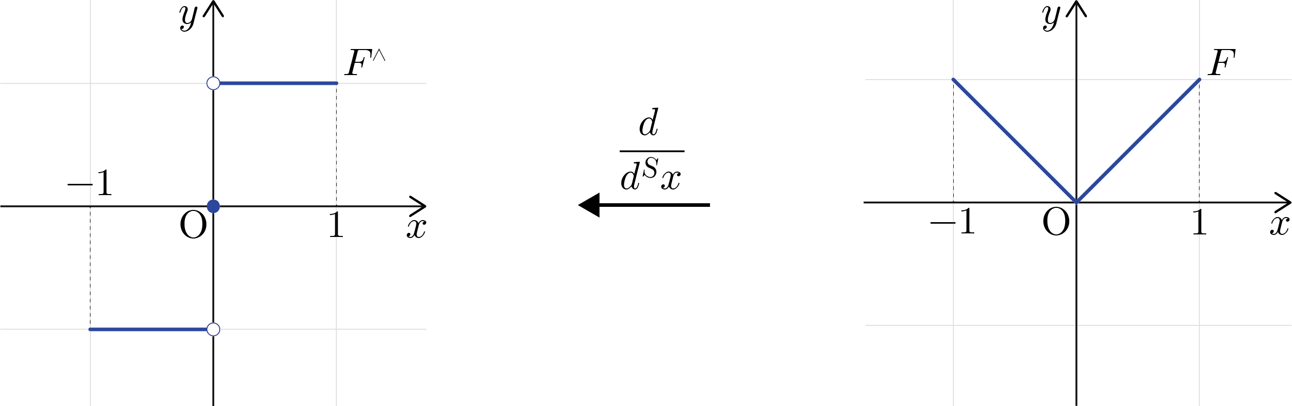
Figure 9: FTC with specular derivatives for the sign function

Motivated by the previous example, we define the indefinite integral of a piecewise continuous function.

Definition 4.3.

Suppose $f:[a,b]\to\mathbb{R}$ be a piecewise continuous function. Let $\left\{s_{1},s_{2},\cdots,s_{k}\right\}$ to be the singular set of $f$. Define $s_{0}:=a$ and $s_{k+1}:=b$. Denote index sets by $\mathcal{I}:=\left\{0,1,\cdots,k\right\}$. For each $i\in\mathcal{I}$, define the function $\overline{f_{i}}:\left[s_{i},s_{i+1}\right]\to\mathbb{R}$ to be the extended function of $f$ on $(s_{i},s_{i+1})$ by

$$\overline{f_{i}}(x_{i}):=\begin{cases}f[s_{i})&\text{if }x_{i}=s_{i},\\ f(x_{i})&\text{if }x_{i}\in(s_{i},s_{i+1}),\\ f(s_{i+1}]&\text{if }x_{i}=s_{i+1}.\end{cases}$$

We define the indefinite integral $F$ of $f$ by

$$F(x):=\begin{cases}\displaystyle\int_{a}^{x}\overline{f_{0}}(t)~{}dt&\text{if }x\in\left[a,s_{1}\right],\\[12.80365pt] \displaystyle\int_{s_{1}}^{x}\overline{f_{1}}(t)~{}dt+\int_{s_{0}}^{s_{1}}\overline{f_{0}}(t)~{}dt&\text{if }x\in\left(s_{1},s_{2}\right],\\[12.80365pt] \displaystyle\int_{s_{2}}^{x}\overline{f_{2}}(t)~{}dt+\sum_{\ell=1}^{2}\int_{s_{\ell-1}}^{s_{\ell}}\overline{f_{\ell-1}}(t)~{}dt&\text{if }x\in\left(s_{2},s_{3}\right],\\ \qquad\qquad\qquad\vdots\\ \displaystyle\int_{s_{k}}^{x}\overline{f_{k}}(t)~{}dt+\sum_{\ell=1}^{k}\int_{s_{\ell-1}}^{s_{\ell}}\overline{f_{\ell-1}}(t)~{}dt&\text{if }x\in\left(s_{k},s_{k+1}\right].\end{cases}$$

The our goal is to suggest and prove the relation, so-called FTC with specular derivatives, between a piecewise continuous function $f$ and specular derivatives $F^{\mathbin{\vbox{\hbox{\scalebox{0.5}{$\bm{\wedge}$}}}}}$ of indefinite integrals $F$ of $f$, that is, $F$ is continuous and

$$\frac{d}{d^{S}x}F(x)=f(x)$$ (4.1)

for $x\in[a,b]$. To achieve this, it needs to examine proper conditions of $f$. Consider the piecewise continuous function $g:[-1,1]\to\mathbb{R}$ defined by

$$g(x)=\begin{cases}-1&\text{if }x\in[-1,0],\\ 1&\text{if }x\in(0,1].\end{cases}$$

Our hope (4.1) fails in light of Proposition 2.15. If the indefinite integral $G$ of $g$ is specularly differentiable at $0$, then $g(0)=0$ according to Proposition 2.15. In other words, $G$ is not specularly differentiable at $0$ since $g(0)=1$. Hence, it is reasonable to assume the following hypothesis for a piecewise continuous function $f:[a,b]\to\mathbb{R}$ in stating FTC with specular derivatives:

1. For each point $x\in(a,b)$, the property

   $$f(x)=\begin{cases}\displaystyle\frac{\alpha\beta-1+\sqrt{\left(\alpha^{2}+1\right)\left(\beta^{2}+1\right)}}{\alpha+\beta}&\text{if }\alpha+\beta\neq 0,\\ 0&\text{if }\alpha+\beta=0,\end{cases}$$

   holds, where $\alpha:=f[x)$ and $\beta:=f(x]$.

As for (H1), it suffices to check only the points at which $f$ has a jump discontinuity. Also, one can assume the following hypotheses instead of (H1) resulted from Lemma 2.21:

1. For each point $x\in(a,b)$, the property

   $$f(x)=\tan\left(\frac{\arctan\alpha+\arctan\beta}{2}\right)$$

   holds, where $\alpha:=f[x)$ and $\beta:=f(x]$.

However, we prefer to assume (H1).

Before stating FTC with specular derivatives, we give an example with a simple periodic function in order to figure out our strategy of the proof.

Example 4.4.

For a fixed $k\in\mathbb{N}$, let $p:[0,k+1]\to\mathbb{R}$ be the periodic function defined by

$$p(x)=\begin{cases}2x&\text{if }x\in[0,1),\\ \displaystyle\frac{-1+\sqrt{5}}{2}&\text{if }x=1,\\[4.0pt] p(x-1)&\text{if }x\in(1,k+1),\\ 2&\text{if }x=k+1,\end{cases}$$

which is illustrated in Figure 10. Note that $p$ meets (H1).

Denote the index sets by $\mathcal{I}:=\left\{0,1,\cdots,k\right\}$ and $\mathcal{J}:=\mathcal{I}\setminus\left\{0\right\}$. For each $i\in\mathcal{I}$, the extended function $\overline{f_{i}}:[i,i+1]\to\mathbb{R}$ is defined by

$$\overline{f_{i}}(x_{i})=\begin{cases}p[i)&\text{if }x_{i}=i,\\ p(x_{i})&\text{if }x_{i}\in(i,i+1),\\ p(i+1]&\text{if }x_{i}=i+1,\end{cases}=2(x_{i}-i)$$

and the indefinite integral of $\overline{f_{i}}$ is defined by

$$F_{i}(x_{i})=\int_{i}^{x_{i}}\overline{f_{i}}(t)~{}dt=\int_{i}^{x_{i}}2(t-i)~{}dt=\left[t^{2}-2it\right]_{t=i}^{x_{i}}=(x_{i}-i)^{2}$$

for $x_{i}\in[i,i+1]$.

Now, observe that the function $F:[0,k+1]\to\mathbb{R}$ defined by

$$F(x)=\begin{cases}x^{2}&\text{if }x\in[0,1],\\ (x-1)^{2}+1&\text{if }x\in(1,2],\\ (x-2)^{2}+2&\text{if }x\in(2,3],\\ \qquad\qquad\qquad\vdots\\ (x-k)^{2}+k&\text{if }x\in(k,k+1],\end{cases}$$

is the indefinite integral $F$ of $p$. For each $i\in\mathcal{I}$, since $\overline{f_{i}}$ is continuous on $[i,i+1]$, FTC asserts that $F_{i}$ is continuous on $[i,i+1]$ with $F_{i}^{\prime}(x_{i})=\overline{f_{i}}(x_{i})$ for all $x_{i}\in[i,i+1]$. Then we have $F(x)$ is continuous and $F^{\prime}(x)=p(x)$ for all $x\in[0,k+1]\setminus\mathcal{J}$.

Moreover, for each $j\in\mathcal{J}$ one can calculate

$$F^{\mathbin{\vbox{\hbox{\scalebox{0.5}{$\bm{\wedge}$}}}}}_{-}(j)=\left.2[x-(j-1)]\right|_{x=j}=2\qquad\text{and}\qquad F^{\mathbin{\vbox{\hbox{\scalebox{0.5}{$\bm{\wedge}$}}}}}_{+}(j)=\left.2(x-j)\right|_{x=j}=0$$

so that

$$F^{\mathbin{\vbox{\hbox{\scalebox{0.5}{$\bm{\wedge}$}}}}}(j)=\frac{-1+\sqrt{5}}{2}=p(j)$$

by using Proposition 2.15. Hence, we have $F^{\mathbin{\vbox{\hbox{\scalebox{0.5}{$\bm{\wedge}$}}}}}(x)\equiv p(x)$ owing to Theorem 2.18.

It suffices to prove that $F$ is continuous on $\mathcal{J}$. Indeed, for each $j\in\mathcal{J}$, observe that

$$F(j)=\left[j-(j-1)\right]^{2}+(j-1)=j=\lim_{x\searrow j}(x-j)^{2}+j=\lim_{x\searrow j}F(x).$$

which means that $F$ is continuous at $x=j$. Consequently, the indefinite integral $F$ is continuous on $[0,k+1]$ and

$$\frac{d}{d^{S}x}\left(\int_{0}^{x}p(t)~{}dt\right)=\frac{d}{d^{S}x}F(x)=p(x)$$

for $x\in[0,k+1]$.

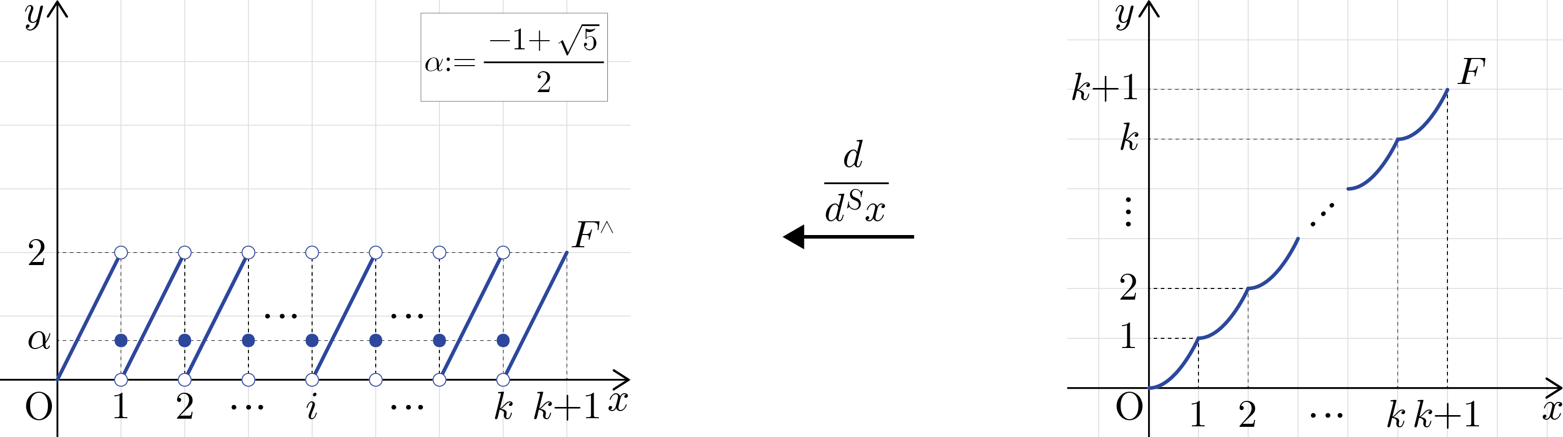
Figure 10: FTC with specular derivatives for the periodic function

Here is the connection between the notions of the specular derivative and the integral.

Theorem 4.5.

(The Fundamental Theorem of Calculus with specular derivatives) Suppose $f:[a,b]\to\mathbb{R}$ be a piecewise continuous function. Assume (H1). Let $F$ be the indefinite integral of $f$. Then the following properties hold:

1. $F$ is continuous on $[a,b]$.

2. $F^{\mathbin{\vbox{\hbox{\scalebox{0.5}{$\bm{\wedge}$}}}}}(x)=f(x)$ for all $x\in[a,b]$.

Proof.

Denote the singular set of $f$ by

$$\mathcal{S}:=\left\{s_{1},s_{2},\cdots,s_{k}\right\}$$

with the index sets $\mathcal{I}:=\left\{0,1,\cdots,k\right\}$ and $\mathcal{J}:=\mathcal{I}\setminus\left\{0\right\}$. For each $i\in\mathcal{I}$, the extended function $\overline{f_{i}}:\left[s_{i},s_{i+1}\right]\to\mathbb{R}$ is defined by

$$\overline{f_{i}}(x_{i})=\begin{cases}f[s_{i})&\text{if }x_{i}=s_{i},\\ f(x_{i})&\text{if }x_{i}\in(s_{i},s_{i+1}),\\ f(s_{i+1}]&\text{if }x_{i}=s_{i+1},\end{cases}$$

and the indefinite integral of $\overline{f_{i}}$ is defined by

$$F_{i}(x_{i})=\int_{s_{i}}^{x_{i}}\overline{f_{i}}(t)~{}dt$$

for $x_{i}\in\left[s_{i},s_{i+1}\right]$.

Now, one can find that the function $F:[a,b]\to\mathbb{R}$ defined by

$$F(x):=\begin{cases}F_{0}(x)&\text{if }x\in[a,s_{1}],\\ F_{1}(x)+F_{0}(s_{1})&\text{if }x\in(s_{1},s_{2}],\\ \displaystyle F_{2}(x)+\sum_{\ell=1}^{2}F_{\ell-1}(s_{\ell})&\text{if }x\in(s_{2},s_{3}],\\ \qquad\qquad\qquad\vdots\\ \displaystyle F_{k}(x)+\sum_{\ell=1}^{k}F_{\ell-1}(s_{\ell})&\text{if }x\in(s_{k},s_{k+1}],\end{cases}$$

is the indefinite integral $F$ of $f$. For each $i\in\mathcal{I}$, since $\overline{f_{i}}$ is continuous on $\left[s_{i},s_{i+1}\right]$, FTC asserts that $F_{i}$ is continuous on $\left[s_{i},s_{i+1}\right]$ with $F_{i}^{\prime}(x_{i})=\overline{f_{i}}(x_{i})$ for all $x_{i}\in\left[s_{i},s_{i+1}\right]$. Then $F(x)$ is continuous and $F^{\prime}(x)=f(x)$ for all $x\in[a,b]\setminus\mathcal{S}$.

Moreover, for each $j\in\mathcal{J}$ one can calculate

$$F^{\mathbin{\vbox{\hbox{\scalebox{0.5}{$\bm{\wedge}$}}}}}_{-}(s_{j})=\left.\frac{d}{d^{L}x}\left(F_{j-1}(x)+\sum_{\ell=1}^{j-1}F_{\ell-1}(s_{\ell})\right)\right|_{x=s_{j}}=\left.\frac{d}{d^{L}x}F_{j-1}(x)\right|_{x=s_{j}}=\left.\frac{d}{d^{L}x}\overline{f_{j-1}}(x)\right|_{x=s_{j}}=f^{\mathbin{\vbox{\hbox{\scalebox{0.5}{$\bm{\wedge}$}}}}}_{-}(s_{j})$$

and

$$F^{\mathbin{\vbox{\hbox{\scalebox{0.5}{$\bm{\wedge}$}}}}}_{+}(s_{j})=\left.\frac{d}{d^{R}x}\left(F_{j}(x)+\sum_{\ell=1}^{j}F_{\ell-1}(s_{\ell})\right)\right|_{x=s_{j}}=\left.\frac{d}{d^{R}x}F_{j}(x)\right|_{x=s_{j}}=\left.\frac{d}{d^{R}x}\overline{f_{j}}(x)\right|_{x=s_{j}}=f^{\mathbin{\vbox{\hbox{\scalebox{0.5}{$\bm{\wedge}$}}}}}_{+}(s_{j}),$$

which implies that $F^{\mathbin{\vbox{\hbox{\scalebox{0.5}{$\bm{\wedge}$}}}}}(s)=f(s)$ for all $s\in\mathcal{S}$ by the assumption (H1). Hence, we have $F^{\mathbin{\vbox{\hbox{\scalebox{0.5}{$\bm{\wedge}$}}}}}\equiv f$ owing to Theorem 2.18.

Lastly, it is enough to prove that $F$ is continuous on $\mathcal{S}$. To show this, for each $j\in\mathcal{J}$, observe that

$$F(s_{j}) =\int_{s_{j-1}}^{s_{j}}\overline{f_{j-1}}(t)~{}dt+\sum_{\ell=1}^{j-1}\int_{s_{\ell-1}}^{s_{\ell}}\overline{f_{\ell-1}}(t)~{}dt$$

$$=\sum_{\ell=1}^{j}\int_{s_{\ell-1}}^{s_{\ell}}\overline{f_{\ell-1}}(t)~{}dt$$

$$=\lim_{x\searrow s_{j}}\int_{s_{j}}^{x}\overline{f_{j}}(t)~{}dt+\sum_{\ell=1}^{j}\int_{s_{\ell-1}}^{s_{\ell}}\overline{f_{\ell-1}}(t)~{}dt$$

$$=\lim_{x\searrow s_{j}}F(x),$$

which means that $F$ is continuous at $x=s_{j}$. In conclusion, the indefinite integral $F$ is continuous on $[a,b]$ and

$$\frac{d}{d^{S}x}\left(\int_{a}^{x}f(t)~{}dt\right)=\frac{d}{d^{S}x}F(x)=f(x)$$

for $x\in[a,b]$. Consequently, we complete the proof. ∎

4.2 Ordinary differential equations with specular derivatives

In this subsection, we deal with an ordinary differential equation (ODE for short) in the specular derivative sense.

Let $U$ be an open set in $\mathbb{R}$ and $x$ be an arbitrary point in $U$. Consider a first order ordinary differential equation with specular derivatives, that is,

$$\frac{du}{d^{S}x}=f(u,x),$$ (4.2)

where $f:U\to\mathbb{R}$ is a given function of two variables and a function $u:U\to\mathbb{R}$ is unknown. We call $u$ is a solution of a first order ODE with specular derivatives (4.2) if $u$ is continuous on $U$ and satisfies (4.2).

In this paper, we study the general first order linear ordinary differential equation with specular derivatives of the form

$$a_{1}(x)u^{\mathbin{\vbox{\hbox{\scalebox{0.5}{$\bm{\wedge}$}}}}}+a_{0}(x)u=g(x),$$

where continuous functions $a_{1}:U\to\mathbb{R}\setminus\left\{0\right\}$, $a_{2}:U\to\mathbb{R}$ and a piecewise function $g:U\to\mathbb{R}$ with the singular set that all singular points are undefined are given. We usually write the standard form of a first order linear ODE with specular derivatives:

$$u^{\mathbin{\vbox{\hbox{\scalebox{0.5}{$\bm{\wedge}$}}}}}+p(x)u=f(x),$$ (4.3)

where a continuous function $p:U\to\mathbb{R}$ and a piecewise continuous function $f:U\to\mathbb{R}$ such that all singular points are unknown are given. As usual, we say that a first order linear ODE with specular derivatives (4.3) is either homogeneous if $f\equiv 0$ or non-homogeneous if $f\not\equiv 0$. Especially, we say that solving a first order linear ODE with specular derivatives is to obtain not only the solution $u$ but also the singular set of $f$.

Here is the reason why we consider the piecewise continuous function not a continuous function. According to Theorem 2.25, if $f$ is continuous on $U$, then the first order linear ODE with specular derivatives is equal with the first order linear ODE with classical derivatives. Indeed, we are not interested in a homogeneous first order linear ODE with specular derivatives. Thus, we assume that $f$ is piecewise continuous function when it comes to a first order linear ODE with specular derivatives. Furthermore, in order to agree with the unknown singular set, note that singular points may directly affect the solutions. We explain the reason later (see Remark 4.8).

Recall first how to solve the first order linear ordinary differential equation with classical derivatives. Let us consider the ODE:

$$u^{\prime}+p(x)u=f(x),$$ (4.4)

where the functions $p:\mathbb{R}\to\mathbb{R}$ and $f:\mathbb{R}\to\mathbb{R}$ are given, and the function $u:\mathbb{R}\to\mathbb{R}$ is the unknown. The function $\mu(x)$ such that

$$\frac{d}{dx}(\mu u)=p(x)\mu(x)$$

is called the integrating factor. Using the integrating factor and the Chain Rule yield the general solution of (4.4) is

$$u=\frac{1}{\mu(x)}\left(\int\mu(t)f(t)dt+C\right)$$

for some constant $C\in\mathbb{R}$ if the functions $f$ and $p$ are continuous. Otherwise, if $f$ or $p$ is a piecewise continuous function, one can find the way to solve the ODE by separating the given domain or by applying the Laplace transform in [3] and [13].

As in Remark 2.17, one cannot generally solve (4.3) by using the function $\mu(x)$, so-called an integrating factor, since

$$\frac{d}{d^{S}x}(\mu u)=\frac{d\mu}{d^{S}x}u+\mu\frac{du}{d^{S}x}$$

may fail. See the following example.

Example 4.6.

Consider the functions $u:(0,2)\to\mathbb{R}$ and $f:(0,2)\to\mathbb{R}$ defined by

$$u(x)=\begin{cases}0&\text{if }x\in(0,1],\\ x-1&\text{if }x\in(1,2),\end{cases}\qquad\text{and}\qquad f(x)=\begin{cases}0&\text{if }x\in(0,1),\\ x&\text{if }x\in(1,2),\end{cases}$$

respectively. Observe that the function $u$ and the singular point $f(1)=-1+\sqrt{2}$ solve the first order linear ODE with specular derivatives:

$$u^{\mathbin{\vbox{\hbox{\scalebox{0.5}{$\bm{\wedge}$}}}}}+u=f(x)$$

for $x\in(0,2)$. However, one can calculate

$$\left.\frac{d}{d^{S}x}\left(e^{x}u\right)\right|_{x=1}=\frac{-1+\sqrt{e^{2}+1}}{e}\neq e(-1+\sqrt{2})=\left.e^{x}u+e^{x}\frac{du}{d^{S}x}\right|_{x=1},$$

using Proposition 2.15. Hence, we have to find out other avenue not using an integrating factor in obtaining the general solution.

Now, we start with a restricted type of non-homogeneous first order linear ODE with specular derivatives:

$$u^{\mathbin{\vbox{\hbox{\scalebox{0.5}{$\bm{\wedge}$}}}}}+cu=f(x),$$ (4.5)

where a constant $c\in\mathbb{R}$ and a piecewise continuous function $f:U\to\mathbb{R}$ such that all singular points are unknown are given. We want to obtain the unknown continuous function $u:U\to\mathbb{R}$ and the singular set of $f$.

Here is the several steps to solve the equation: First, we separate the given equation based on the points at which $f$ has a jump discontinuity. Next, by Proposition 2.24, the separated equations are first order linear ODE with classical derivatives can be solved as usual. Third, the solutions are matched so that $u$ is continuous at which $f$ has a jump discontinuity by finding proper constants. Finally, the singular set of $f$ can be found by applying Proposition 2.15 or Lemma 2.21.

Example 4.7.

Let $f:\mathbb{R}\to\mathbb{R}$ be the function defined by

$$f(x)=\begin{cases}0&\text{if }x<0,\\ 3x+1&\text{if }x>0.\end{cases}$$

Consider the first order linear ODE with specular derivatives:

$$u^{\mathbin{\vbox{\hbox{\scalebox{0.5}{$\bm{\wedge}$}}}}}+3u=f(x)$$ (4.6)

for $x\in\mathbb{R}$. We want to obtain the solution $u$ and the value $f(0)$.

We first solve the equation separately for $x<0$ and $x>0$:

$$u^{\prime}+3u=\begin{cases}0&\text{if }x<0,\\ 3x+1&\text{if }x>0,\end{cases}$$

by Proposition 2.24. Using the intergrating factor $\mu(x)=e^{3x}$, the solutions are

$$u(x)=\begin{cases}C_{1}e^{-3x}&\text{if }x<0,\\ x+C_{2}e^{-3x}&\text{if }x>0,\end{cases}$$

for some constants $C_{1}$ and $C_{2}$ in $\mathbb{R}$, respectively. In order to match the two solutions so that $u$ is continuous at $0$, the calculation

$$u(0]=\lim_{x\nearrow 0}C_{1}e^{-3x}=C_{1}=C_{2}=\lim_{x\searrow 0}\left(x+C_{2}e^{-3x}\right)=u[0)$$

yields $u(0)=C_{1}=C_{2}=:C$. Hence, we obtain the solution of the given ODE with specular derivatives (4.6)

$$u(x)=\begin{cases}Ce^{-3x}&\text{if }x<0,\\ C&\text{if }x=0,\\ x+Ce^{-3x}&\text{if }x>0,\end{cases}$$

for some constant $C\in\mathbb{R}$. Also, the singular point is

$$f(0)=\begin{cases}\displaystyle\frac{9C^{2}+1-\sqrt{\left(9C^{2}+1\right)\left(9C^{2}-6C+2\right)}}{6C-1}&\displaystyle\text{if }C\neq\frac{1}{6},\\[12.80365pt] \displaystyle\frac{1}{2}&\displaystyle\text{if }C=\frac{1}{6},\end{cases}$$

by Proposition 2.15. Note that the solution is the ReLU function with $f(0)=-1+\sqrt{2}$ if $C=0$.

We explain the delayed motivation for the given piecewise continuous function $f$ which has the undefined singular set.

Remark 4.8.

The reason why we assume that every singular point of $f$ is undefined is in that the singular points affect not only the existence and but also the uniqueness of the solution. Consider Example 4.7. Write the function $\varphi:\mathbb{R}\to\mathbb{R}$ defined by $\varphi(C)=u^{\mathbin{\vbox{\hbox{\scalebox{0.5}{$\bm{\wedge}$}}}}}(0)+3C-f(0)$ for $C\in\mathbb{R}$, i.e.,

$$\varphi(C)=\begin{cases}\displaystyle\frac{9C^{2}+1-\sqrt{\left(9C^{2}+1\right)\left(9C^{2}-6C+2\right)}}{6C-1}-f(0)&\displaystyle\text{if }C\neq\frac{1}{6},\\[12.80365pt] \displaystyle\frac{1}{2}-f(0)&\displaystyle\text{if }C=\frac{1}{6}.\end{cases}$$

On the one hand, assume $f(0)=-1+\sqrt{2}$ is given. Then the equation $\varphi(C)=0$ has two solutions $C=0$ and $C=-\frac{2}{3}$. Hence, the solutions of the given ODE (4.6) are only

$$u_{1}(x)=\begin{cases}0&\text{if }x\leq 0,\\ x&\text{if }x>0,\end{cases}\qquad\text{and}\qquad u_{2}(x)=\begin{cases}\displaystyle-\frac{2}{3}e^{-3x}&\text{if }x\leq 0,\\[12.80365pt] \displaystyle x-\frac{2}{3}e^{-3x}&\text{if }x>0.\end{cases}$$

On the other hand, assume $f(0)=0$ is given. Then the equation $\varphi(C)=0$ has no solution. Hence, there is no solution of the given ODE (4.6). In conclusion, to achieve well-posedness concerning the existence and the uniqueness, the piecewise continuous function $f$ has to be undefined on the singular set unless each singular point is the given value.

To solve a first order linear ODE with specular derivatives (4.3) is akin to the way solving ODE with specular derivatives (4.5). Hence, we suggest the following theorem without any examples.

Theorem 4.9.

The non-homogeneous first order linear ODE with specular derivatives (4.3) has a solution.

Proof.

Denote the singular set of $f$ by

$$\mathcal{S}:=\left\{s_{1},s_{2},\cdots,s_{k}\right\}$$

with the index sets $\mathcal{I}:=\left\{0,1,\cdots,k\right\}$ and $\mathcal{J}:=\mathcal{I}\setminus\left\{0\right\}$. Denote the end points of the open set $U=(a,b)$ by $s_{0}:=a$ and $s_{k+1}:=b$ (possibly $a=-\infty$ or $b=\infty$). Since $p$ is continuous on $U$, there exists an integrating factor

$$\mu(x)=\exp\left(\int p(x)~{}dx\right)$$

such that $\mu^{\prime}(x)=p(x)\mu(x)$ for all $x\in U$. Then the function

$$u(x)=\begin{cases}\displaystyle\frac{1}{\mu(x)}\left(\int_{s_{0}}^{x}\mu(t)f(t)~{}dt+C_{0}\right)&\text{if }x\in(s_{0},s_{1}),\\[12.80365pt] \displaystyle\frac{1}{\mu(x)}\left(\int_{s_{1}}^{x}\mu(t)f(t)~{}dt+C_{1}\right)&\text{if }x\in(s_{1},s_{2}),\\[12.80365pt] \qquad\qquad\qquad\vdots&\\[12.80365pt] \displaystyle\frac{1}{\mu(x)}\left(\int_{s_{k}}^{x}\mu(t)f(t)~{}dt+C_{k}\right)&\text{if }x\in(s_{k},s_{k+1}),\end{cases}$$

is the solutions of the separated equations.

For each $j\in\mathcal{J}$, to achieve that $u$ is continuous at $s_{j}$, we calculate

$$u(s_{j}]=\frac{1}{\mu(s_{j})}\left(\int_{s_{j-1}}^{s_{j}}\mu(t)f(t)~{}dt+C_{j-1}\right)=\frac{1}{\mu(s_{j})}C_{j}=\frac{1}{\mu(s_{j})}\left(\int_{s_{j}}^{s_{j}}\mu(t)f(t)~{}dt+C_{j}\right)=u[s_{j}),$$

which implies that

$$C_{j}=\int_{s_{j-1}}^{s_{j}}\mu(t)f(t)~{}dt+C_{j-1}$$ (4.7)

defined inductively. Hence, for each $j\in\mathcal{J}$, $u$ is continuous at $x=s_{j}$ as well as $u(s_{j})=C_{j}$.

Since for each $j\in\mathcal{J}$ there exist $u^{\prime}_{+}(s_{j})$ and $u^{\prime}_{-}(s_{j})$, one can compute the value $f(s_{j})$ by using Proposition 2.15 or Lemma 2.21. Consequently, we conclude that $u$ is a solution of the given ODE with specular derivatives (4.3). ∎

Corollary 4.10.

The non-homogeneous first order linear ODE with specular derivatives (4.3) with the given value at a single point $x_{0}\in U$ has the unique solution.

Proof.

Assume $s_{1}$, $s_{2}$, $\cdots$, $s_{k}$ are elements of the singular set of $f$. Denote the end points of the open set $U=(a,b)$ by $s_{0}:=a$ and $s_{k+1}:=b$ (possibly $a=-\infty$ or $b=\infty$). Assume the value $u(x_{0})=y_{0}$ is given. Then $x_{0}\in(s_{i},s_{i+1})$ for some $i\in\left\{0,1,\cdots,k\right\}$. In the proof of Theorem 4.9, the given value determines the constant $C_{i}$ as the fixed real number. The undetermined constants are inductively determined thanks to (4.7). Clearly, the all constants are unique, which implies the solution of the ODE with specular derivatives (4.3) is unique. ∎

One can weaken the continuous function $p$ to be piecewise continuous. In this case, the given domain has to be more complicatedly separated.

4.3 Partial differential equations with specular derivatives

In this subsection, we address a partial differential equation (PDE for short) in light of specular derivatives.

Consider the PDE called the transport equation with specular derivatives:

$$\partial^{S}_{t}u+\mathbf{b}\mathbin{\vbox{\hbox{\scalebox{0.5}{$\bullet$}}}}D^{S}_{\mathbf{x}}u=c\chi_{\left\{\mathbf{x}=t\mathbf{b}\right\}}\quad\text{in }\mathbb{R}^{n}\times(0,\infty),$$ (4.8)

where the vector $\mathbf{b}\in\mathbb{R}^{n}$ and the constant $c\in\mathbb{R}$ are given, the function $u:\mathbb{R}^{n}\times[0,\infty)\to\mathbb{R}$ is the unknown with $u=u(\mathbf{x},t)=u(x_{1},\cdots,x_{n},t)$, and $\chi_{A}:\mathbb{R}^{n}\times(0,\infty)\to\left\{0,1\right\}$ is the characteristic function of a subset $A\subset\mathbb{R}^{n}\times(0,\infty)$ defined by

$$\chi_{A}(\mathbf{x},t)=\begin{cases}1&\text{if }(\mathbf{x},t)\in A,\\ 0&\text{if }(\mathbf{x},t)\notin A.\end{cases}$$

Here the spatial variable $\mathbf{x}=(x_{1},x_{2},\cdots,x_{n})\in\mathbb{R}^{n}$ and the time variable $t\geq 0$ denote a typical point in space and time, respectively.

From now on, we deal with the PDE (4.8) with the certain initial-value: the generalized ReLU function. Here, we state the initial-value problem with specular derivatives:

$$\begin{cases}\begin{aligned} \displaystyle\partial^{S}_{t}u+\mathbf{b}\mathbin{\vbox{\hbox{\scalebox{0.5}{$\bullet$}}}}D^{S}_{\mathbf{x}}u&=c\chi_{\left\{\mathbf{x}=t\mathbf{b}\right\}},&&\text{in }\mathbb{R}^{n}\times(0,\infty),\\ u&=g&&\text{on }\mathbb{R}^{n}\times\left\{t=0\right\},\end{aligned}\end{cases}$$ (4.9)

where the function $g:\mathbb{R}^{n}\to\mathbb{R}$ defined by

$$g(\mathbf{x})=\begin{cases}a_{1}(x_{1}+x_{2}+\cdots+x_{n})&\text{if }x_{1}+x_{2}+\cdots+x_{n}\geq 0,\\ a_{2}(x_{1}+x_{2}+\cdots+x_{n})&\text{if }x_{1}+x_{2}+\cdots+x_{n}<0,\end{cases}$$ (4.10)

is given with fixed constants $a_{1}$, $a_{2}\in\mathbb{R}$. Here $\mathbf{x}=(x_{1},x_{2},\cdots,x_{n})\in\mathbb{R}^{n}$ denotes a typical point in space, and $t\geq 0$ denotes a typical time.

Recall the PDE, so-called the transport equation, with constant coefficients and the initial-value:

$$\begin{cases}\begin{aligned} \displaystyle u_{t}+\mathbf{b}\mathbin{\vbox{\hbox{\scalebox{0.5}{$\bullet$}}}}D_{\mathbf{x}}u&=f&&\text{in }\mathbb{R}^{n}\times(0,\infty),\\ u&=g&&\text{on }\mathbb{R}^{n}\times\left\{t=0\right\},\end{aligned}\end{cases}$$ (4.11)

where the vector $\mathbf{b}\in\mathbb{R}^{n}$ and the functions $f:\mathbb{R}^{n}\times(0,\infty)\to\mathbb{R}$, $g:\mathbb{R}^{n}\to\mathbb{R}$ are given, and the function $u:\mathbb{R}^{n}\times[0,\infty)\to\mathbb{R}$ is the unknown with $u=u(\mathbf{x},t)=u(x_{1},x_{2},\cdots,x_{n},t)$. Here $\mathbf{x}=(x_{1},x_{2},\cdots,x_{n})\in\mathbb{R}^{n}$ and $t\geq 0$ denotes a typical point in space and a typical time, respectively. The solution of the initial value-problem (4.11) is

$$u(\mathbf{x},t)=g(\mathbf{x}-t\mathbf{b})+\int_{0}^{t}f(\mathbf{x}+(s-t)\mathbf{b},s)ds$$

for $\mathbf{x}\in\mathbb{R}^{n}$ and $t\geq 0$. The Chain Rule is used in solving the PDE (4.11). The detailed explanation is in [8].

First of all, we try to solve the equation for a one-dimensional spatial variable, that is,

$$\begin{cases}\begin{aligned} \displaystyle\partial^{S}_{t}u+b\partial^{S}_{x}u&=c\chi_{\left\{x=tb\right\}}&&\text{in }\mathbb{R}\times(0,\infty),\\ u&=g&&\text{on }\mathbb{R}\times\left\{t=0\right\},\end{aligned}\end{cases}$$ (4.12)

where constants $b$, $c\in\mathbb{R}$ are given, the function $u:\mathbb{R}\times[0,\infty)\to\mathbb{R}$ is the unknown with $u=u(x,t)$, the $\chi_{A}$ is the characteristic function of a set $A\subset\mathbb{R}\times(0,\infty)$, and the function $g:\mathbb{R}\to\mathbb{R}$ defined by

$$g(x)=\begin{cases}a_{1}x&\text{if }x\geq 0,\\ a_{2}x&\text{if }x<0,\end{cases}$$ (4.13)

is given with fixed constants $a_{1}$, $a_{2}\in\mathbb{R}$. Here $x\in\mathbb{R}$ denotes a typical point in space, and $t\geq 0$ denotes a typical time. The above setting can be illustrated as follows.

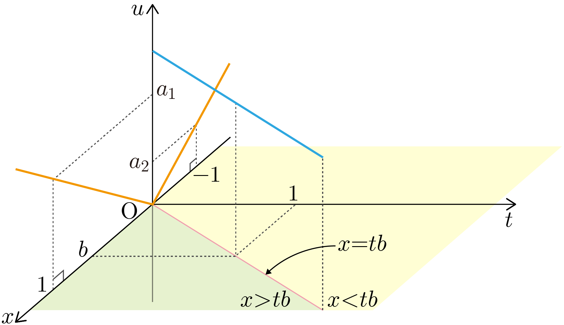
Figure 11: The setting for the initial-value problem with specular derivatives

Note that the function $g$ can be regarded as the generalized ReLU function by substituting zero in place of $a_{2}$. When we solve the transport equation with classical derivatives, the Chain Rule plays a crucial role. However, as for specular derivatives, the Chain Rule may fail (see Remark 2.17).

If $x=tb$, as we solve the transport equation in the classical derivative sense, one can find the incomplete solution of (4.12) is

$$u(x,t)=\begin{cases}a_{1}(x-tb)&\text{if }x>tb,\\ a_{2}(x-tb)&\text{if }x<tb.\end{cases}$$

Now, assume $x=tb$. Then we calculate that

$$\partial^{R}_{t}u=-a_{1}b,~{}\partial^{L}_{t}u=-a_{2}b\qquad\text{and}\qquad\partial^{R}_{x}u=a_{1},~{}\partial^{L}_{x}u=a_{2}.$$

Applying Proposition 2.15, one can compute that

$$\partial^{S}_{t}u=0=\partial^{S}_{x}u$$

if $a_{1}+a_{2}=0$ as well as

$$\partial^{S}_{t}u=\frac{a_{1}a_{2}b^{2}-1+\sqrt{\left(a_{1}^{2}b^{2}+1\right)\left(a_{2}^{2}b^{2}+1\right)}}{-(a_{1}+a_{2})b}\qquad\text{and}\qquad\partial^{S}_{x}u=\frac{a_{1}a_{2}-1+\sqrt{\left(a_{1}^{2}+1\right)\left(a_{2}^{2}+1\right)}}{a_{1}+a_{2}}$$

if $a_{1}+a_{2}\neq 0$. In any cases, the equality $\partial^{S}_{t}u+b\partial^{S}_{x}u=c$ must be held. Therefore, we deduce a solution of (4.12) exists provided $c$ satisfies the equality

$$c=\begin{cases}\displaystyle\frac{1-\sqrt{\left(a_{1}^{2}b^{2}+1\right)\left(a_{2}^{2}b^{2}+1\right)}-b^{2}\left(1-\sqrt{\left(a_{1}^{2}+1\right)\left(a_{2}^{2}+1\right)}\right)}{(a_{1}+a_{2})b}&\text{if }a_{1}+a_{2}\neq 0,\\[12.80365pt] 0&\text{if }a_{1}+a_{2}=0.\end{cases}$$ (4.14)

Consequently, since the values of the $u(x,t)$ on $\left\{x=tb\right\}$ do not affect specular derivatives on $\left\{x=tb\right\}$, a solution of (4.12) is

$$u(x,t)=\begin{cases}a_{1}(x-tb)&\text{if }x\geq tb,\\ a_{2}(x-tb)&\text{if }x<tb.\end{cases}$$

For instance, consider the initial-value problem

$$\begin{cases}\begin{aligned} \displaystyle 10\partial^{S}_{t}u+20\partial^{S}_{x}u&=\left(4\sqrt{34}-5\sqrt{13}-3\right)\chi_{\left\{x=2t\right\}}&&\text{in }\mathbb{R}\times(0,\infty),\\ u&=g&&\text{on }\mathbb{R}\times\left\{t=0\right\},\end{aligned}\end{cases}$$ (4.15)

where

$$g(x)=\begin{cases}4x&\text{if }x\geq 0,\\ x&\text{if }x<0.\end{cases}$$

Then the solution of (4.15) exists since $\displaystyle c=\frac{1}{10}\left(4\sqrt{34}-5\sqrt{13}-3\right)$ satisfies the equation (4.14) and is

$$u(x,t)=\begin{cases}4(x-2t)&\text{if }x\geq 2t,\\ x-2t&\text{if }x<2t.\end{cases}$$

As for high-dimensional spatial variables, the initial-value problem (4.9) has a solution provided the equation

$$c=\begin{cases}\displaystyle\frac{a_{1}a_{2}b^{2}-1+\sqrt{\left(a_{1}^{2}b^{2}+1\right)\left(a_{2}^{2}b^{2}+1\right)}}{-(a_{1}+a_{2})b}+b^{n}n\left(\frac{a_{1}a_{2}-1+\sqrt{\left(a_{1}^{2}+1\right)\left(a_{2}^{2}+1\right)}}{a_{1}+a_{2}}\right)&\text{if }a_{1}+a_{2}\neq 0,\\[12.80365pt] 0&\text{if }a_{1}+a_{2}=0,\end{cases}$$

holds and the solution is

$$u(\mathbf{x},t)=\begin{cases}a_{1}(\mathbf{x}-tb)&\text{if }\mathbf{x}\geq tb,\\ a_{2}(\mathbf{x}-tb)&\text{if }\mathbf{x}<tb.\end{cases}$$

5 Appendix

5.1 Delayed proofs

In this subsection, we provide the proof of Proposition 2.15, Corollary 2.16, and Lemma 2.21.

5.1.1 Proof of Proposition 2.15

Note that specular derivatives do not depend on the translation or radius of circles in the definition.

Proof.

Without loss of generality, suppose $f[0]=0$. Write $f^{\mathbin{\vbox{\hbox{\scalebox{0.5}{$\bm{\wedge}$}}}}}_{+}(0)=:\alpha_{0}$ and $f^{\mathbin{\vbox{\hbox{\scalebox{0.5}{$\bm{\wedge}$}}}}}_{-}(0)=:\beta_{0}$. From (2.2), we get

$$a_{0}=\frac{r}{\sqrt{\alpha_{0}^{2}+1}}\qquad\text{and}\qquad b_{0}=-\frac{r}{\sqrt{\beta_{0}^{2}+1}}$$

as the roots between the circle centered at the origin with radius $r>0$ and $\operatorname{pht}f$ at $x=0$. Denote the intersection points of the unit circle centered at the origin and $\operatorname{pht}f$ at $x=0$ by $\text{A}=(a_{0},\operatorname{pht}f(a_{0}))$ and $\text{B}=(b_{0},\operatorname{pht}f(b_{0}))$, i.e.,

$$\text{A}=\left(\frac{r}{\sqrt{\alpha_{0}^{2}+1}},\frac{r\alpha_{0}}{\sqrt{\alpha_{0}^{2}+1}}\right)\qquad\text{and}\qquad\text{B}=\left(-\frac{r}{\sqrt{\beta_{0}^{2}+1}},-\frac{r\beta_{0}}{\sqrt{\beta_{0}^{2}+1}}\right).$$

Since $f^{\mathbin{\vbox{\hbox{\scalebox{0.5}{$\bm{\wedge}$}}}}}(0)$ is equal with the slope of the line AB, we find that

$$f^{\mathbin{\vbox{\hbox{\scalebox{0.5}{$\bm{\wedge}$}}}}}(0) =\frac{\operatorname{pht}f(a_{0})-\operatorname{pht}f(b_{0})}{a_{0}-b_{0}}$$

$$=\left(\frac{\beta_{0}\sqrt{\alpha_{0}^{2}+1}+\alpha_{0}\sqrt{\beta_{0}^{2}+1}}{\sqrt{\left(\alpha_{0}^{2}+1\right)\left(\beta_{0}^{2}+1\right)}}\right)\left(\frac{{\sqrt{\left(\alpha_{0}^{2}+1\right)\left(\beta_{0}^{2}+1\right)}}}{\sqrt{\alpha_{0}^{2}+1}+\sqrt{\beta_{0}^{2}+1}}\right)$$

$$=\frac{\beta_{0}\sqrt{\alpha_{0}^{2}+1}+\alpha_{0}\sqrt{\beta_{0}^{2}+1}}{\sqrt{\alpha_{0}^{2}+1}+\sqrt{\beta_{0}^{2}+1}}.$$

If $\alpha_{0}+\beta_{0}=0$, it is obvious that $f^{\mathbin{\vbox{\hbox{\scalebox{0.5}{$\bm{\wedge}$}}}}}(0)=0$. Now, assume $\alpha_{0}+\beta_{0}\neq 0$. Then, we calculate that

$$f^{\mathbin{\vbox{\hbox{\scalebox{0.5}{$\bm{\wedge}$}}}}}(0) =\frac{\left(\beta_{0}\sqrt{\alpha_{0}^{2}+1}+\alpha_{0}\sqrt{\beta_{0}^{2}+1}\right)\left(\sqrt{\alpha_{0}^{2}+1}-\sqrt{\beta_{0}^{2}+1}\right)}{\alpha_{0}^{2}-\beta_{0}^{2}}$$

$$=\frac{\beta_{0}\left(\alpha_{0}^{2}+1\right)-\alpha_{0}\left(\beta_{0}^{2}+1\right)+\left(\alpha_{0}-\beta_{0}\right)\sqrt{\left(\alpha_{0}^{2}+1\right)\left(\beta_{0}^{2}+1\right)}}{\alpha_{0}^{2}-\beta_{0}^{2}}$$

$$=\frac{\alpha_{0}\beta_{0}\left(\alpha_{0}-\beta_{0}\right)-\left(\alpha_{0}-\beta_{0}\right)+\left(\alpha_{0}-\beta_{0}\right)\sqrt{\left(\alpha_{0}^{2}+1\right)\left(\beta_{0}^{2}+1\right)}}{\left(\alpha_{0}-\beta_{0}\right)\left(\alpha_{0}+\beta_{0}\right)}$$

$$=\frac{\alpha_{0}\beta_{0}-1+\sqrt{\left(\alpha_{0}^{2}+1\right)\left(\beta_{0}^{2}+1\right)}}{\alpha_{0}+\beta_{0}},$$

as required. ∎

5.1.2 Useful lemma

Let us introduce the temporary notation for the function $A:U\to\mathbb{R}$ defined by

$$A(\alpha,\beta):=\frac{\alpha\beta-1+\sqrt{\left(\alpha^{2}+1\right)\left(\beta^{2}+1\right)}}{\alpha+\beta}$$

for $(\alpha,\beta)\in U$, which comes from Proposition 2.15, where the domain of the function $A$ is

$$U=\left\{(\alpha,\beta)\in\mathbb{R}\times\mathbb{R}:\alpha+\beta\neq 0\right\}.$$

Analysis for this function can be useful in proving various properties of specular derivatives: Corollary 2.16, Corollary 3.24, and Theorem 3.25.

Lemma 5.1.

For every $(\alpha,\beta)\in U$, the following statements hold:

1. $A(\alpha,\beta)\neq 0$.

2. Signs of $\alpha+\beta$ and $A(\alpha,\beta)$ are equal, i.e., $\operatorname{sgn}(\alpha+\beta)=\operatorname{sgn}(A(\alpha,\beta))$.

3. $\displaystyle-\frac{\left|\alpha+\beta\right|}{2}\leq A(\alpha,\beta)\leq\frac{\left|\alpha+\beta\right|}{2}$.

Proof.

First of all, we prove (i). Assume $(\alpha,\beta)\in U$. Let $\alpha$, $\beta$ be real numbers with $\alpha+\beta\neq 0$. Suppose to the contrary that $A(\alpha,\beta)=0$. Calculating that

$$\left(\alpha^{2}+1\right)\left(\beta^{2}+1\right)=1+\alpha^{2}\beta^{2}-2\alpha\beta,$$

we find that $\alpha+\beta=0$, which implies that $(\alpha,\beta)\notin U$, a contradiction. Hence, we conclude that $A(\alpha,\beta)\neq 0$.

Next, to show (ii) and (iii), let $(\alpha,\beta)$ be an element of the domain $U$. The application of the Arithmetic Mean-Geometric Mean Inequality for $\alpha^{2}+1>0$ and $\beta^{2}+1>0$ implies that

$$\sqrt{\left(\alpha^{2}+1\right)\left(\beta^{2}+1\right)}\leq\frac{\alpha^{2}+\beta^{2}}{2}+1$$

and then we have

$$\alpha\beta-1+\sqrt{\left(\alpha^{2}+1\right)\left(\beta^{2}+1\right)}\leq\frac{(\alpha+\beta)^{2}}{2}.$$ (5.1)

Moreover, note that $(\alpha+\beta)^{2}\geq 0$ since $(\alpha,\beta)\in U$. This inequality implies that $\alpha\beta-1+\sqrt{\left(\alpha^{2}+1\right)\left(\beta^{2}+1\right)}\geq 0$. Combining with (5.1), we have

$$0\leq\alpha\beta-1+\sqrt{\left(\alpha^{2}+1\right)\left(\beta^{2}+1\right)}\leq\frac{(\alpha+\beta)^{2}}{2}.$$ (5.2)

Now, dividing the left inequality of (5.2) by $\alpha+\beta$, one can find that (ii). Furthermore, dividing the right inequality of (5.2) by $\left|\alpha+\beta\right|$, we obtain

$$\left|A(\alpha,\beta)\right|=\frac{\alpha\beta-1+\sqrt{\left(\alpha^{2}+1\right)\left(\beta^{2}+1\right)}}{\left|\alpha+\beta\right|}\leq\frac{\left|\alpha+\beta\right|}{2},$$

which yields (iii), completing the proof. ∎

5.1.3 Proof of Lemma 2.21

Proof.

Write $\alpha:=f^{\mathbin{\vbox{\hbox{\scalebox{0.5}{$\bm{\wedge}$}}}}}_{+}(x_{0})$, $\beta:=f^{\mathbin{\vbox{\hbox{\scalebox{0.5}{$\bm{\wedge}$}}}}}_{-}(x_{0})$ and $\gamma:=f^{\mathbin{\vbox{\hbox{\scalebox{0.5}{$\bm{\wedge}$}}}}}(x_{0})$. First of all, suppose $\alpha+\beta=0$. Then Proposition 2.15 implies that

$$\tan\theta=\gamma=0=\alpha+\beta=\tan\theta_{1}+\tan\theta_{2}.$$

On the one hand, $\theta=0$. On the other hand, observing that

$$0=\frac{\tan\theta_{1}+\tan\theta_{2}}{1-\tan\theta_{1}\tan\theta_{2}}=\tan(\theta_{1}+\theta_{2}),$$

we conclude that

$$\frac{1}{2}(\theta_{1}+\theta_{2})=0=\theta,$$

completing the proof for the case $\alpha+\beta=0$.

Next, assume $\alpha+\beta\neq 0$. Using Proposition 2.15, we have

$$\gamma=\frac{\alpha\beta-1+\sqrt{\left(\alpha^{2}+1\right)\left(\beta^{2}+1\right)}}{\alpha+\beta},$$

which implies that the second order equation with respect to $\gamma$.

$$(\alpha+\beta)\gamma^{2}+2(1-\alpha\beta)\gamma-(\alpha+\beta)=0.$$

Using this equation, observe that

$$\tan(2\theta)=\frac{2\tan\theta}{1-\tan^{2}\theta}=\frac{2\gamma}{1-\gamma^{2}}=\frac{\alpha+\beta}{1-\alpha\beta}=\frac{\tan\theta_{1}+\tan\theta_{2}}{1-\tan\theta_{1}\tan\theta_{2}}=\tan(\theta_{1}+\theta_{2}),$$

which yields $2\theta=\theta_{1}+\theta_{2}$, as required. ∎

5.2 Notation

Let $f:\mathbb{R}\to\mathbb{R}$ be a single-variable function and let $x$ denotes a typical point in $\mathbb{R}$. Also, let $g:\mathbb{R}^{n}\to\mathbb{R}$ be a multi-variable function with $n\in\mathbb{N}$ and let $\mathbf{x}=(x_{1},\cdots,x_{n})$ denotes a typical point in $\mathbb{R}^{n}$. We denote $x_{i}$ to indicate the $i$-th component of the vector $\mathbf{x}$. Lastly, let $k$ be a positive integer. In this paper, we employ the following notation:

	Classical derivative	Specular derivative
$\mathbb{R}\to\mathbb{R}$	$\displaystyle f^{\prime}_{+}\quad\text{and}\quad f^{\prime}_{-}$	$\displaystyle D^{R}f=D^{R}_{x}f=\frac{df}{d^{R}f}=f^{\mathbin{\vbox{\hbox{\scalebox{0.5}{$\bm{\wedge}$}}}}}_{+}\quad\text{and}\quad D^{L}f=D^{L}_{x}f=\frac{df}{d^{L}f}=f^{\mathbin{\vbox{\hbox{\scalebox{0.5}{$\bm{\wedge}$}}}}}_{-}$
	$\displaystyle Df=D_{x}f=\frac{df}{dx}=f^{\prime}=\dot{f}$, $\displaystyle\frac{d^{k}f}{dx^{k}}=f^{(k)}$	$\displaystyle D^{S}f=D^{S}_{x}f=\frac{df}{d^{S}x}=f^{\mathbin{\vbox{\hbox{\scalebox{0.5}{$\bm{\wedge}$}}}}}$, $\displaystyle\left(D^{S}\right)^{k}f=\left(D^{S}_{x}\right)^{k}f=\frac{d^{k}f}{d^{S}x^{k}}=f^{[k]}$
$\mathbb{R}^{n}\to\mathbb{R}$	$-$	$\displaystyle\partial^{R}_{x_{i}}g=\frac{\partial g}{\partial^{R}x_{i}}\quad\text{and}\quad\partial^{L}_{x_{i}}g=\frac{\partial g}{\partial^{L}x_{i}}$
	$\displaystyle\partial_{x_{i}}g=\frac{\partial g}{\partial x_{i}}=g_{x_{i}}$, $\displaystyle\partial^{k}_{x_{i}}g=\frac{\partial^{k}g}{\partial x^{k}_{i}}$	$\displaystyle\partial^{S}_{x_{i}}g=\frac{\partial g}{\partial^{S}x_{i}}$, $\displaystyle\left(\partial^{S}_{x_{i}}\right)^{k}g=\frac{\partial^{k}g}{\partial^{S}x^{k}_{i}}$
	$\displaystyle\partial_{\mathbf{u}}f=D_{\mathbf{u}}f=\nabla_{\mathbf{u}}f$	$\displaystyle\partial^{S}_{\mathbf{u}}f$
	$-$	$\displaystyle D^{R}f=D_{\mathbf{x}}^{R}f\quad\text{and}\quad D^{L}f=D_{\mathbf{x}}^{L}f$
	$Df=D_{\mathbf{x}}f=\nabla f$	$D^{S}f=D_{\mathbf{x}}^{S}f$

Table 1: Notation for classical and specular derivatives

References

- [1] C. E. Aull. The first symmetric derivative. Amer. Math. Monthly, 74:708–711, 1967.
- [2] R. G. Bartle and D. R. Sherbert. Introduction to Real Analysis. John Wiley & Sons, Inc., New York, 4th edition, 2011.
- [3] W. E. Boyce, R. C. DiPrima, and D. B. Meade. Elementary differential equations and boundary value problems. John Wiley & Sons, Inc., New York, 11th edition, 2017.
- [4] A. Bressan. Lecture notes on functional analysis, volume 143 of Graduate Studies in Mathematics. American Mathematical Society, Providence, RI, 2013.
- [5] A. M. Bruckner. Differentiation of real functions, volume 5 of CRM Monograph Series. American Mathematical Society, Providence, RI, 2nd edition, 1994.
- [6] A. M. Bruckner and J. L. Leonard. Derivatives. Amer. Math. Monthly, 73:24–56, 1966.
- [7] S. J. Colley. Vector calculus. Pearson, Boston, 4th edition, 2012.
- [8] L. C. Evans. Partial differential equations, volume 19 of Graduate Studies in Mathematics. American Mathematical Society, Providence, RI, 2nd edition, 2010.
- [9] L. Larson. The symmetric derivative. Trans. Amer. Math. Soc., 277(2):589–599, 1983.
- [10] P. K. Sahoo. Quasi-mean value theorems for symmetrically differentiable functions. Tamsui Oxf. J. Inf. Math. Sci., 27(3):279–301, 2011.
- [11] P. K. Sahoo and T. Riedel. Mean value theorems and functional equations. World Scientific Publishing Co., Inc., River Edge, NJ, 1998.
- [12] H. Whitney. Analytic extensions of differentiable functions defined in closed sets. Trans. Amer. Math. Soc., 36(1):63–89, 1934.
- [13] D. G. Zill. A first course in differential equations with modeling applications. Cengage Learning, Boston, 11th edition, 2018.