Reinforcement Learning with
Automated Auxiliary Loss Search

Abstract

A good state representation is crucial to solving complicated reinforcement learning (RL) challenges. Many recent works focus on designing auxiliary losses for learning informative representations. Unfortunately, these handcrafted objectives rely heavily on expert knowledge and may be sub-optimal. In this paper, we propose a principled and universal method for learning better representations with auxiliary loss functions, named Automated Auxiliary Loss Search (A2LS), which automatically searches for top-performing auxiliary loss functions for RL. Specifically, based on the collected trajectory data, we define a general auxiliary loss space of size $7.5\times 10^{20}$ and explore the space with an efficient evolutionary search strategy. Empirical results show that the discovered auxiliary loss (namely, A2-winner) significantly improves the performance on both high-dimensional (image) and low-dimensional (vector) unseen tasks with much higher efficiency, showing promising generalization ability to different settings and even different benchmark domains. We conduct a statistical analysis to reveal the relations between patterns of auxiliary losses and RL performance. The codes and supplementary materials are available at https://seqml.github.io/a2ls.

1 Introduction

Reinforcement learning (RL) has achieved remarkable progress in games [31, 47, 50], financial trading [8] and robotics [13]. However, in its core part, without designs tailored to specific tasks, general RL paradigms are still learning implicit representations from critic loss (value predictions) and actor loss (maximizing cumulative reward). In many real-world scenarios where observations are complicated (e.g., images) or incomplete (e.g., partial observable), training an agent that is able to extract informative signals from those inputs becomes incredibly sample-inefficient.

Therefore, many recent works have been devoted to obtaining a good state representation, which is believed to be one of the key solutions to improve the efficacy of RL [23, 24]. One of the main streams is adding auxiliary losses to update the state encoder. Under the hood, it resorts to informative and dense learning signals in order to encode various prior knowledge and regularization [40], and obtain better latent representations. Over the years, a series of works have attempted to figure out the form of the most helpful auxiliary loss for RL. Quite a few advances have been made, including observation reconstruction [51], reward prediction [20], environment dynamics prediction [40, 6, 35], etc. But we note two problems in this evolving process: (i) each of the loss designs listed above are obtained through empirical trial-and-errors based on expert designs, thus heavily relying on human labor and expertise; (ii) few works have used the final performance of RL as an optimization objective to directly search the auxiliary loss, indicating that these designs could be sub-optimal. To resolve the issues of the existing handcrafted solution mentioned above, we decide to automate the process of designing the auxiliary loss functions of RL and propose a principled solution named Automated Auxiliary Loss Search (A2LS). A2LS formulates the problem as a bi-level optimization where we try to find the best auxiliary loss, which, to the most extent, helps train a good RL agent. The outer loop searches for auxiliary losses based on RL performance to ensure the searched losses align with the RL objective, while the inner loop performs RL training with the searched auxiliary loss function. Specifically, A2LS utilizes an evolutionary strategy to search the configuration of auxiliary losses over a novel search space of size $7.5\times 10^{20}$ that covers many existing solutions. By searching on a small set of simulated training environments of continuous control from Deepmind Control suite (DMC) [43], A2LS finalizes a loss, namely A2-winner.

To evaluate the generalizability of the discovered auxiliary loss A2-winner, we test A2-winner on a wide set of test environments, including both image-based and vector-based (with proprioceptive features like positions, velocities and accelerations as inputs) tasks. Extensive experiments show the searched loss function is highly effective and largely outperforms strong baseline methods. More importantly, the searched auxiliary loss generalizes well to unseen settings such as (i) different robots of control; (ii) different data types of observation; (iii) partially observable settings; (iv) different network architectures; and (v) even to a totally different discrete control domain (Atari 2600 games [1]). In the end, we make detailed statistical analyses on the relation between RL performance and patterns of auxiliary losses based on the data of whole evolutionary search process, providing useful insights on future studies of auxiliary loss designs and representation learning in RL.

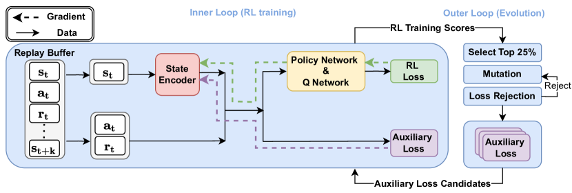
Figure 1: Overview of A2LS. A2LS contains an inner loop (left) and an outer loop (right). The inner loop performs an RL training procedure with searched auxiliary loss functions. The outer loop searches auxiliary loss functions using an evolutionary algorithm to select the better auxiliary losses.

2 Problem Formulation and Background

We consider the standard Markov Decision Process (MDP) $\mathcal{E}$ where the state, action and reward at time step $t$ are denoted as $(s_{t},a_{t},r_{t})$. The sequence of rollout data sampled by the agent in the episodic environment is $({s_{0},\ldots,s_{t},a_{t},r_{t},s_{t+1},\cdots,s_{T}})$, where $T$ represents the episode length. Suppose the RL agent is parameterized by $\omega$ (either the policy $\pi$ or the state-action value function $Q$), with a state encoder $g_{\theta}$ parameterized by $\theta\subseteq\omega$ which plays a key role for representation learning in RL. The agent is required to maximize its cumulative rewards in environment $\mathcal{E}$ by optimizing $\omega$, noted as $\mathcal{R}(\omega;\mathcal{E})=\mathbb{E}_{\pi}[\sum_{t=0}^{T-1}r_{t}]$.

In this paper, we aim to find the optimal auxiliary loss function $\mathcal{L}_{\text{Aux}}$ such that the agent can reach the best performance by optimizing $\omega$ under a combination of an arbitrary RL loss function $\mathcal{L}_{\text{RL}}$ together with an auxiliary loss $\mathcal{L}_{\text{Aux}}$. Formally, our optimization goal is:

$$\max_{\mathcal{L}_{\text{Aux}}}\quad\mathcal{R}(\min_{\omega}\mathcal{L}_{\text{RL}}(\omega;\mathcal{E})+\lambda\mathcal{L}_{\text{Aux}}(\theta;\mathcal{E});\mathcal{E})~{},$$ (1)

where $\lambda$ is a hyper-parameter balancing the relative weight of the auxiliary loss. The left part (inner loop) of Figure 1 illustrates how data and gradients flow in RL training when an auxiliary loss is enabled. Some instances of $\mathcal{L}_{\text{RL}}$ and $\mathcal{L}_{\text{Aux}}$ are given in Appendix B. Unfortunately, existing auxiliary losses $\mathcal{L}_{\text{Aux}}$ are handcrafted, which heavily rely on expert knowledge, and may not generalize well in different scenarios as shown in the experiment part. To find better auxiliary loss functions for representation learning in RL, we introduce our principled solution in the following section.

3 Automated Auxiliary Loss Search

To meet our goal of finding top-performing auxiliary loss functions without expert assignment, we turn to the help of automated loss search, which has shown promising results in the automated machine learning (AutoML) community [27, 28, 48]. Correspondingly, we propose Automated Auxiliary Loss Search (A2LS), a principled solution for resolving the above bi-level optimization problem in Equation 1. A2LS resolves the inner problem as a standard RL training procedure; for the outer one, A2LS defines a finite and discrete search space (Section 3.1), and designs a novel evolution strategy to efficiently explore the space (Section 3.2).

Table 1: Typical solution with auxiliary loss and their common elements.

Auxiliary Loss	Operator	Input Elements
		Horizon	Source	Target
Forward dynamics [35, 40, 6]	MSE	1	$\{s_{t},a_{t}\}$	$\{s_{t+1}\}$
Inverse dynamics	MSE	1	$\{a_{t},s_{t+1}\}$	$\{s_{t}\}$
Reward prediction [20, 6]	MSE	1	$\{s_{t},a_{t}\}$	$\{r_{t}\}$
Action inference [40, 6]	MSE	1	$\{s_{t},s_{t+1}\}$	$\{a_{t}\}$
CURL [23]	Bilinear	1	$\{s_{t}\}$	$\{s_{t}\}$
ATC [42]	Bilinear	k	$\{s_{t}\}$	$\{s_{t+1},\cdots,s_{t+k}\}$
SPR [39]	N-MSE	k	$\{s_{t},a_{t},a_{t+1},\cdots,a_{t+k-1}\}$	$\{s_{t+1},\cdots,s_{t+k}\}$

3.1 Search Space Design

We have argued that almost all existing auxiliary losses require expert knowledge, and we expect to search for a better one automatically. To this end, it is clear that we should design a search space that satisfies the following desiderata.

• Generalization: the search space should cover most of the existing handcrafted auxiliary losses to ensure the searched results can be no worse than handcrafted losses;

• Atomicity: the search space should be composed of several independent dimensions to fit into any general search algorithm [30] and support an efficient search scheme;

• Sufficiency: the search space should be large enough to contain the top-performing solutions.

Given the criteria, we conclude and list some existing auxiliary losses in Table 1 and find their commonalities, as well as differences. We realize that these losses share similar components and computation flow. As shown in Figure 2, when training the RL agent, the loss firstly selects a sequence $\{s_{t},a_{t},r_{t}\}_{t=i}^{i+k}$ from the replay buffer, when $k$ is called horizon. The agent then tries to predict some elements in the sequence (called target) based on another picked set of elements from the sequence (called source). Finally, the loss calculates and minimizes the prediction error (rigorously defined with operator). To be more specific, the encoder part $g_{\theta}$ of the agent, first encodes the source into latent representations, which is further fed into a predictor $h$ to get a prediction $y$; the auxiliary loss is computed by the prediction $y$ and the target $\hat{y}$ that is translated from the target by a target encoder $g_{\hat{\theta}}$, using an operator $f$. The target encoder is updated in an momentum manner as shown in Figure 2 (details are given in Section C.1.2). Formally,

$$\mathcal{L}_{\text{Aux}}(\theta;\mathcal{E})=f\Big{(}h\big{(}g_{\theta}(\text{seq}_{\text{source}})\big{)},g_{\hat{\theta}}(\text{seq}_{\text{target}})\Big{)}~{},$$ (2)

where $\text{seq}_{\text{source}},\text{seq}_{\text{target}}\subseteq\{s_{t},a_{t},r_{t}\}_{t=i}^{i+k}$ are both subsets of the candidate sequence. And for simplicity, we will denote $g_{\theta}(s_{t},a_{t},r_{t},s_{t+1},\cdots)$ as short for $[g_{\theta}(s_{t}),a_{t},r_{t},g_{\theta}(s_{t+1}),\cdots]$ for the rest of this paper (the encoder $g$ only deals with states $\{s_{i}\}$). Thereafter, we observe that these existing auxiliary losses differ in two dimensions, i.e., input elements and operator, where input elements are further combined by horizon, source and target. These differences compose our search dimensions of the whole space. We then illustrate the search ranges of these dimensions in detail.

Input elements.

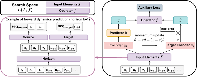
Figure 2: Overview of the search space $\{\mathcal{I},f\}$ and the computation graph of auxiliary loss functions. $\mathcal{I}$ selects a candidate sequence $\{s_{t},a_{t},r_{t}\}_{t=i}^{i+k}$ with horizon $k$; then determine a source and a target as arbitrary subsets of the sequence; an encoder $g_{\theta}$ first encodes the source into latent representations, which is fed into a predictor $h$ to get a prediction $y$; the auxiliary loss is computed over the prediction $y$ and the ground truth $\hat{y}$ that is translated from the target by a target encoder $g_{\hat{\theta}}$, using a operator $f$.

The input elements denote all inputs to the loss functions, which can be further disassembled as horizon, source and target. Different from previous automated loss search works, the target here is not “ground-truth” because auxiliary losses in RL have no labels beforehand. Instead, both source and target are generated via interacting with the environment in a self-supervised manner. Particularly, the input elements first determine a candidate sequence $\{s_{t},a_{t},r_{t}\}_{t=i}^{i+k}$ with horizon $k$. Then, it chooses two subsets from the candidate sequence as source and target respectively. For example, the subsets can be $\{s_{t}\},\{s_{t},s_{t+1}\}$, or $\{s_{t},r_{t+1},a_{t+2}\},\{s_{t},s_{t+1},a_{t+1}\}$, etc.

Operator. Given a prediction $y$ and its target $\hat{y}$, the auxiliary loss is computed by an operator $f$, which is often a similarity measure. In our work, we cover all different operators $f$ used by the previous works, including inner product (Inner) [17, 42], bilinear inner product (Bilinear) [23], cosine similarity (Cosine) [3], mean squared error (MSE) [35, 6] and normalized mean squared error (N-MSE) [39]. Additionally, other works also utilize contrastive objectives, e.g., InfoNCE loss [33], incorporating the trick to sample un-paired predictions and targets as negative samples and maximize the distances between them. This technique is orthogonal to the five similarity measures mentioned above, so we make it optional and create $5\times 2=10$ different operators in total.

Final design. In the light of preceding discussion, with the definition of input elements and operator, we finish the design of the search space, which satisfactorily meets the desiderata mentioned above. Specifically, the space is generalizable to cover most of the existing handcrafted auxiliary losses; additionally, the atomicity is embodied by the compositionality that all input elements work with any operator; most importantly, the search space is sufficiently large with a total size of $7.5\times 10^{20}$ (detailed calculation can be found in Appendix E) to find better solutions.

3.2 Search Strategy

The success of evolution strategies in exploring large, multi-dimensional search space has been proven in many works [19, 4]. Similarly, A2LS adopts an evolutionary algorithm [37] to search for top-performing auxiliary loss functions over the designed search space. In its essence, the evolutionary algorithm (i) keeps a population of loss function candidates; (ii) evaluates their performance; (iii) eliminates the worst and evolves into a new better population. Note that step (ii) of “evaluating” is very costly because it needs to train the RL agents with dozens of different auxiliary loss functions. Therefore, our key technical contribution contains how to further reduce the search cost (Section 3.2.1) and how to make an efficient search procedure (Section 3.2.2).

3.2.1 Search Space Pruning

In our preliminary experiment, we find out the dimension of operator in the search space can be simplified. In particular, MSE outperforms all the others by significant gaps in most cases. So we effectively prune other choices of operators except MSE. See Section D.1 for complete comparative results and an ablation study on the effectiveness of search space pruning.

3.2.2 Evolution Procedure

Our evolution procedure roughly contains four important components: (i) evaluation and selection: a population of candidate auxiliary losses is evaluated through an inner loop of RL training, then we select the top candidates for the next evolution stage (i.e., generation); (ii) mutation: the selected candidates mutate to form a new population and move to the next stage; (iii) loss rejection: filter out and skip evaluating invalid auxiliary losses for the next stage; and (iv) bootstrapping initial population: assign more chance to initial auxiliary losses that may contain useful patterns by prior knowledge for higher efficiency. The step-by-step evolution algorithm is provided in Algorithm 1 in the appendix, and an overview of the A2LS pipeline is illustrated in Figure 1. We next describe them in detail.

Evaluation and selection. At each evolution stage, we first train a population of candidates with a population size $P=100$ by the inner loop of RL training. The candidates are then sorted by computing the approximated area under learning curve (AULC) [11, 41], which is a single metric reflecting both the convergence speed and the final performance [46] with low variance of results. After each training stage, the top-25% candidates are selected to generate the population for the next stage. We include an ablation study on the effectiveness of AULC in Section D.3.

Mutation. To obtain a new population of auxiliary loss functions, we propose a novel mutation strategy. First, we represent both the source and the target of the input elements as a pair of binary masks, where each bit of the mask represents selected by 1 or not selected by 0. For instance, given a candidate sequence $\{s_{t},a_{t},r_{t},s_{t+1},a_{t+1},r_{t+1}\}$, the binary mask of this subset sequence $\{s_{t},a_{t},r_{t+1}\}$ is denoted as $110001$. Afterward, we adopt four types of mutations, also shown in Figure 3: (i) replacement (50% of the population): flip the given binary mask with probability $p=\frac{1}{2\cdot(3k+3)}$ with the horizon length $k$; (ii) crossover (20%): generate a new candidate by randomly combining the mask bits of two candidates with the same horizon length in the population; (iii) horizon decrease and horizon increase (10%): append new binary masks to the tail or delete existing binary masks at the back. (iv) random generation (20%): every bit of the binary mask is generated from a Bernoulli distribution $\mathcal{B}(0.5)$.

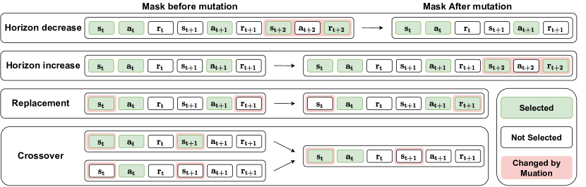
Figure 3: Four types of mutation strategy for evolution. We represent both the source and the target of the input elements as a pair of binary masks, where each bit of the binary mask represents selected (green block) by 1 or not selected (white block) by 0.

Loss rejection protocol. Since the auxiliary loss needs to be differentiable with respect to the parameters of the state encoder, we perform a gradient flow check on randomly generated loss functions during evolution and skip evaluating invalid auxiliary losses. Concretely, the following conditions must be satisfied to make a valid loss function: (i) having at least one state element in $\text{seq}_{\text{source}}$ to make sure the gradient of auxiliary loss can propagate back to the state encoder; (ii) $\text{seq}_{\text{target}}$ is not empty; (iii) the horizon should be within a reasonable range ($1\leq k\leq 10$ in our experiments). If a loss is rejected, we repeat the mutation to fill the population.

Bootstrapping initial population. To improve the computational efficiency so that the algorithm can find reasonable loss functions quickly, we incorporate prior knowledge into the initialization of the search. Particularly, before the first stage of evolution, we bootstrap the initial population with a prior distribution that assigns high probability to auxiliary loss functions containing useful patterns like dynamics and reward prediction. More implementation details are provided in Section C.3.

4 Evolution and Searched Results

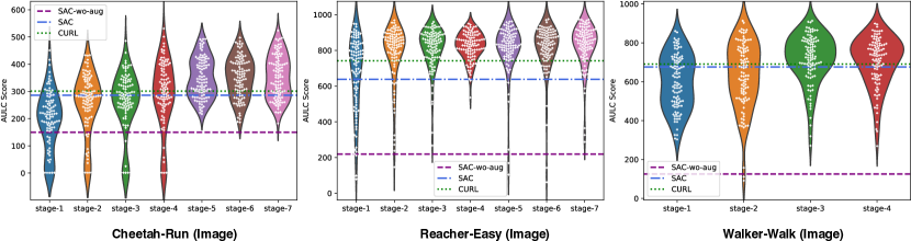
Figure 4: Evolution process in the three training (image-based) environments. Every white dot represents a candidate of auxiliary loss, and y-axis shows its corresponding approximated AULC score [11, 41]. The horizontal lines show the scores of the baselines. The AULC score is approximated with the average evaluation score at 100k, 200k, 300k, 400k, 500k time steps.

As mentioned in Section 1, we expect to find auxiliary losses that align with the RL objective and generalize well to unseen test environments. To do so, we use A2LS to search over a small set of training environments, and then test the searched results on a wide range of test environments. In this section, we first introduce the evolution on training environments and search results.

4.1 Evolution on Training Environments

The training environments are chosen as three image-based (observations for agents are images) continuous control tasks in DMC benchmark [43], Cheetah-Run, Reacher-Easy, and Walker-Walk. For each environment, we set the total budget to 16k GPU hours (on NVIDIA P100) and terminate the search when the resource is exhausted. Due to computation complexity, we only run one seed for each inner loop RL training, but we try to prevent such randomness by cross validation (see Section 4.2). We use the same network architecture and hyperparameters config as CURL [23] (see Section C.4.1 for details) to train the RL agents. To evaluate the population during evolution, we measure A2LS as compared to SAC, SAC-wo-aug, and CURL, where we randomly crop images from $100\times 100$ to $84\times 84$ as data augmentation (the same technique used in CURL[23]) for all methods except SAC-wo-aug. The whole evolution process on three environments is demonstrated in Figure 4. Even in the early stages (e.g., stage 1), some of the auxiliary loss candidates already surpass baselines, indicating the high potential of automated loss search. The overall AULC scores of the population continue to improve when more stages come in (detailed numbers are summerized in Section D.10). Judging from the trend, we believe the performances could improve even more if we had further increased the budget.

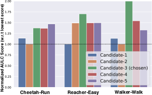
Figure 5: Cross validation on image-based training environments.

4.2 Searched Results: A2-winner

Although some candidates in the population have achieved remarkable AULC scores in the evolution (Figure 4), they were only evaluated with one random seed in one environment, making their robustness under question. To ensure that we find a consistently-useful auxiliary loss, we conduct a cross validation. We first choose the top 5 candidates of stage-5 of the evolution on Cheetah-Run (detailed top candidates during the whole evolution procedure are provided in Appendix F). For each of the five candidates, we repeat the RL training on all three training environments, shown in Figure 5. Finally, we mark the best among five (green bar in Figure 5) as our final searched result. We call it A2-winner, which has the following form:

$$\mathcal{L}_{\text{Aux}}(\theta;\mathcal{E})=\|h\big{(}g_{\theta}(s_{t+1},a_{t+1},a_{t+2},a_{t+3})\big{)}-g_{\hat{\theta}}(r_{t},r_{t+1},s_{t+2},s_{t+3})\|_{2}~{}.$$ (3)

5 Generalization Experiments

To verify the effectiveness of the searched results, we conduct various generalization experiments on a wide range of test environments in depth. Implementation details and more ablation studies are given in Appendix C and Appendix D.

Generalize to unseen image-based tasks. We first investigate the generalizability of A2-winner to unseen image-based tasks by training agents with A2-winner on common DMC tasks and compare with model-based and model-free baselines that use different auxiliary loss functions (see Section C.5 for details about baseline methods). The results are summarized in Table 2 where A2-winner greatly outperforms other baseline methods on most tasks, including unseen test environments. This implies that A2-winner is a robust and effective auxiliary loss for image-based continuous control tasks to improve both the efficiency and final performance.

Table 2: Episodic rewards (mean & standard deviation for 10 seeds) on DMC100K (100K time steps) and DMC500K (500K time steps). Note that the optimal score of DMC is 1000 for all environments. The baseline methods are PlaNet [16], Dreamer [15], SAC+AE [51], SLAC [26], image-based SAC [14]. Performance values of all baselines are referred to [23], except for Image SAC. Learning curves of all 12 DMC environments are included in Section D.2.

500K Steps Scores	A2-winner	CURL§	PlaNet§	Dreamer§	SAC+AE§	SLACv1§	Image SAC
Cheetah-Run†	613 $\pm$ 39	$518\pm 28$	$305\pm 131$	$570\pm 253$	$550\pm 34$	640 $\pm$ 19	99 $\pm$ 28
Reacher-Easy†	938 $\pm$ 46	$929\pm 44$	$210\pm 390$	$793\pm 164$	$627\pm 58$	-	312 $\pm$ 132
Walker-Walk†	917 $\pm$ 18	$902\pm 43$	$351\pm 58$	$897\pm 49$	$847\pm 48$	$842\pm 51$	76 $\pm$ 44
Finger-Spin∗	983 $\pm$ 4	$926\pm 45$	$561\pm 284$	$796\pm 183$	$884\pm 128$	$673\pm 92$	282 $\pm$ 102
Cartpole-Swingup∗	864 $\pm$ 19	$841\pm 45$	$475\pm 71$	$762\pm 27$	$735\pm 63$	-	344 $\pm$ 104
Ball in cup-Catch∗	970 $\pm$ 8	$959\pm 27$	$460\pm 380$	$897\pm 87$	$794\pm 58$	$852\pm 71$	200 $\pm$ 114
100K Steps Scores
Cheetah-Run†	449 $\pm$ 34	$299\pm 48$	$138\pm 88$	$235\pm 137$	$267\pm 24$	$319\pm 56$	128 $\pm$ 12
Reacher-Easy†	778 $\pm$ 164	$538\pm 223$	$20\pm 50$	$314\pm 155$	$274\pm 14$	-	277 $\pm$ 69
Walker-Walk†	510 $\pm$ 151	$403\pm 24$	$224\pm 48$	$277\pm 12$	$394\pm 22$	$361\pm 73$	127 $\pm$ 28
Finger-Spin∗	872 $\pm$ 27	$767\pm 56$	$136\pm 216$	$341\pm 70$	$740\pm 64$	$693\pm 141$	160 $\pm$ 138
Cartpole-Swingup∗	815 $\pm$ 66	$582\pm 146$	$297\pm 39$	$326\pm 27$	$311\pm 11$	-	243 $\pm$ 19
Ball in cup-Catch∗	862 $\pm$ 167	$769\pm 43$	$0\pm 0$	$246\pm 174$	$391\pm 82$	$512\pm 110$	100 $\pm$ 90

• ${\dagger}$: Training environments. $*$: Unseen test environments. $\S$: Results reported in  [23].

Table 3: Mean and Median scores (normalized by human score and random score) achieved by A2LS and baselines on 26 Atari games benchmarked at 100k time-steps (Atari100k).

Metric	A2-winner	CURL	Eff. Rainbow	DrQ [22]	Random	Human
Mean Human-Norm’d	0.568	0.381	0.285	0.357	0.000	1.000
Median Human-Norm’d	0.317	0.175	0.161	0.268	0.000	1.000

Generalize to totally different benchmark domains. To further verify the generalizability of A2-winner on totally different benchmark domains other than DMC tasks, we conduct experiments on the Atari 2600 Games [1], where we take Efficient Rainbow [44] as the base RL algorithm and add A2-winner to obtain a better state representation. Results are shown in Table 3 where A2-winner outperforms all baselines, showing strong evidence of the generalization and potential usages of A2-winner. Note that the base RL algorithm used in Atari is a value-based method, indicating that A2-winner generalizes well to both value-based and policy-based RL algorithms.

r 100K Steps Scores A2-winner A2-winner-v SAC-Identity SAC CURL Cheetah-Run^† 529 $\pm$ 76 472 $\pm$ 30 237 $\pm$ 27 172 $\pm$ 29 190 $\pm$ 32 Finger-Spin^∗ 790 $\pm$ 128 837 $\pm$ 52 805 $\pm$ 32 785 $\pm$ 106 712 $\pm$ 83 Finger-Turn hard^∗ 272 $\pm$ 149 218 $\pm$ 117 347 $\pm$ 150 174 $\pm$ 94 43 $\pm$ 42 Cartpole-Swingup^∗ 866 $\pm$ 24 877 $\pm$ 5 873 $\pm$ 10 866 $\pm$ 7 854 $\pm$ 17 Cartpole-Swingup sparse^∗ 634 $\pm$ 226 695 $\pm$ 147 455 $\pm$ 359 627 $\pm$ 307 446 $\pm$ 196 Reacher-Easy^∗ 818 $\pm$ 211 934 $\pm$ 38 697 $\pm$ 192 874 $\pm$ 87 749 $\pm$ 183 Walker-Stand^∗ 935 $\pm$ 32 948 $\pm$ 7 940 $\pm$ 10 862 $\pm$ 196 767 $\pm$ 104 Walker-Walk^∗ 932 $\pm$ 39 906 $\pm$ 78 873 $\pm$ 89 925 $\pm$ 22 852 $\pm$ 64 Walker-Run^∗ 616 $\pm$ 52 564 $\pm$ 45 559 $\pm$ 34 403 $\pm$ 43 289 $\pm$ 61 Ball in cup-Catch^∗ 964 $\pm$ 7 965 $\pm$ 7 954 $\pm$ 12 962 $\pm$ 13 941 $\pm$ 32 Fish-Upright^∗ 586 $\pm$ 128 498 $\pm$ 88 471 $\pm$ 62 400 $\pm$ 62 295 $\pm$ 117 Hopper-Stand^∗ 177 $\pm$ 257 311 $\pm$ 177 14 $\pm$ 16 26 $\pm$ 40 6 $\pm$ 3 1,000K Steps Scores A2-winner-v A2-winner SAC-Identity SAC CURL Quadruped-Run^† 863 $\pm$ 50 838 $\pm$ 58 345 $\pm$ 157 707 $\pm$ 148 497 $\pm$ 128 Hopper-Hop^† 213 $\pm$ 31 278 $\pm$ 106 121 $\pm$ 51 134 $\pm$ 93 60 $\pm$ 22 Pendulum-Swingup^∗ 200 $\pm$ 322 579 $\pm$ 410 506 $\pm$ 374 379 $\pm$ 391 363 $\pm$ 366 Humanoid-Stand^∗ 329 $\pm$ 35 286 $\pm$ 15 9 $\pm$ 2 7 $\pm$ 1 7 $\pm$ 1 Humanoid-Walk^∗ 311 $\pm$ 36 299 $\pm$ 55 16 $\pm$ 28 2 $\pm$ 0 2 $\pm$ 0 Humanoid-Run^∗ 75 $\pm$ 37 88 $\pm$ 2 1 $\pm$ 0 1 $\pm$ 0 1 $\pm$ 0 ${\dagger}$: Training environments. $*$: Unseen test environments.

Table 4: Episodic rewards (mean & standard deviation for 10 seeds) on DMC100K (easy tasks) and DMC1000K (difficult tasks) with vector inputs.

Generalize to different observation types. To see whether A2-winner (searched in image-based environments) is able to generalize to the environments with different observation types, we test A2-winner on vector-based (inputs for RL agents are proprioceptive features such as positions, velocities and accelerations) tasks of DMC and list the results in Table 4. Concretely, we compare A2-winner with SAC-Identity, SAC and CURL, where SAC-Identity does not have state encoder while the others share the same state encoder architecture (See Section C.1.1 and Section D.6 for detailed implementations). To our delight, A2-winner still outperforms all baselines in 12 out of 18 environments, showing A2-winner can also benefit RL performance in vector-based observations. Moreover, the performance gain is particularly significant in more complex environments like Humanoid, where SAC barely learns anything at 1000K time steps. In order to get a deeper understanding of this phenomenon, we additionally visualize the Q loss landscape for both methods in Section D.7.

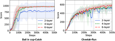
Figure 6: Comparison of A2-winner with different depth of convolutional encoder in image-based DMC environments.

Generalize to different hypothesis spaces.

The architecture of a neural network defines a hypothesis space of functions to be optimized. During the evolutionary search in Section 4.1, the encoder architecture has been kept static as a 4-layer convolutional neural network. Since encoder architecture may have a large impact on the RL training process [34, 2], we test A2-winner with three encoders with different depth of neural networks. The result is shown in Figure 6. Note that even though the auxiliary loss is searched with a 4-layer encoder, the 6-layer convolutional encoder is able to perform better in both two environments. This proves that the auxiliary loss function of A2-winner is able to improve RL performance with a deeper and more expressive image encoder. Moreover, the ranking of RL performance (6-layer > 4-layer > 2-layer) is consistent across the two environments. This shows that the auxiliary loss function of A2-winner does not overfit one specific architecture of the encoder.

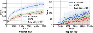
Figure 7: Comparison of A2-winner and baselines in partially observable vector-based DMC environments.

Generalize to partially observable scenarios.

Claiming the generality of a method based on conclusions drawn just on fully observable environments like DMC is very dangerous. Therefore, we conduct an ablation study on the Partially Observable Markov Decision Process (POMDP) setting to see whether A2-winner is able to perform well in POMDP. We random mask 20% of the state dimensions (e.g., 15 dimensions -> 12 dimensions) to form a POMDP environment in DMC. As demonstrated in Figure 7, A2-winner consistently outperforms CURL and SAC-DenseMLP in the POMDP setting in Hopper-Hop and Cheetah-Run, showing that A2-winner is not only effective in fully observable environments but also partially observable environments.

To search or not? As shown above, the searched result A2-winner can generalize well to all kinds of different settings. A natural question here is, however, for a new type of domain, why not perform a new evolution search, instead of simply using the previously searched result? To compare these two solutions, we conduct another evolutionary search similar to Section 4.1 but replaced the three image-based tasks with three vector-based ones (marked by ${\dagger}$ in Table 4) from scratch. More details are summarized in Section D.5. We name the searched result as “A2-winner-v”. As shown in Table 4, A2-winner-v is a very strong-performing loss for vector-based tasks, even stronger than A2-winner. Actually, A2-winner-v is able to outperform baselines in 16 out of 18 environments (with 15 unseen test environments), while A2-winner only outperforms baselines in 12 out of 18 environments. However, please note that it costs another 5k GPU hours (on NVIDIA P100) to search for A2-winner-v while there is no additional cost to directly use A2-winner. It is a trade-off between lower computational cost and better performance.

6 Analysis of Auxiliary Loss Functions

In this section, we analyze all the loss functions we have evaluated during the evolution procedure as a whole dataset in order to gain some insights into the role of auxiliary loss in RL performance. By doing so, we hope to shed light on future auxiliary loss designs. We will also release this “dataset” publicly to facilitate future research.

Typical patterns. We say that an auxiliary loss candidate has a certain pattern if the pattern’s source is a subset of the candidate’s source, and the pattern’s target is a subset of the candidate’s target. For instance, a loss candidate of $\bm{\{s_{t},a_{t}\}\rightarrow\{s_{t+1},s_{t+2}\}}$ has the pattern $\{s_{t},a_{t}\}\rightarrow\{s_{t+1}\}$, and does not have the pattern $\{a_{t},s_{t+1}\}\rightarrow\{s_{t}\}$. We then try to analyze whether a certain pattern is helpful to representation learning in RL in expectation.

Specifically, we analyze the following patterns: (i) forward dynamics $\{s_{t},a_{t}\}\rightarrow\{s_{t+1}\}$; (ii) inverse dynamics $\{a_{t},s_{t+1}\}\rightarrow\{s_{t}\}$; (iii) reward prediction $\{s_{t},a_{t}\}\rightarrow\{r_{t}\}$; (iv) action inference $\{s_{t},s_{t+1}\}\rightarrow\{a_{t}\}$ and (v) state reconstruction in the latent space $\{s_{t}\}\rightarrow\{s_{t}\}$. For each of these patterns, we categorize all the loss functions we have evaluated into (i) with or (ii) without this pattern. We then calculate the average RL performances of these two categories, summarized in Table 5. Some interesting observations are as follows.

• Forward dynamics is helpful in most tasks and improves RL performance on Reacher-Easy (image) and Cheetah-Run (vector) significantly (p-value$<$0.05).

• State reconstruction in the latent space improves RL performance in image-based tasks but undermines vector-based tasks. The improvements in image-based tasks could be attributed to the combination of augmentation techniques, which, combined with reconstruction loss, enforces the extraction of meaningful features. In contrast, no augmentation is used in the vector-based setting, and thus the encoder learns no useful representations. This also explains why CURL performs poorly in vector-based experiments.

• In the vector-based setting, some typical human-designed patterns (e.g., reward prediction, inverse dynamics, and action inference) can be very detrimental to RL performance, implying that some renowned techniques in loss designs might not work well under atypical settings.

Table 5: Statistical analysis on auxiliary loss functions. The number reported is the difference of the expected RL score when the auxiliary losses have one pattern compared to those do not have. The corresponding p-value from the t-test is also reported. Positive numbers indicate that this pattern is beneficial. If the performance gain is statistically significant, the number is marked with the asterisk, indicating it is very likely to be helpful. Negative numbers indicate this pattern is detrimental.

	The score difference between average performances w/ and w/o typical patterns (w/ - w/o)
	Forward dynamics	Inverse dynamics	Reward prediction	Action inference	State reconstruction
Cheetah-Run (Image)	$+1.28~{}~{}~{}~{}~{}$	$-3.51~{}~{}~{}~{}~{}$	$-31.16^{**}~{}~{}$	$-75.95^{**}~{}~{}$	$+42.44^{**}~{}~{}$
Reacher-Easy (Image)	$+28.25^{*}~{}~{}~{}$	$+8.36~{}~{}~{}~{}~{}$	$+37.80^{**}~{}~{}$	$+3.35~{}~{}~{}~{}~{}$	$+70.72^{**}~{}~{}$
Walker-Walk (Image)	$+22.20~{}~{}~{}~{}$	$-48.59^{**}~{}~{}$	$-8.11~{}~{}~{}~{}~{}$	$+29.86^{*}~{}~{}~{}$	$+13.93~{}~{}~{}~{}$
Cheetah-Run (Vector)	$+94.18^{**}~{}~{}$	$-23.66^{**}~{}~{}$	$-33.28^{**}~{}~{}$	$-109.33^{**}~{}$	$-50.15^{**}~{}~{}$
Hopper-Hop (Vector)	$+15.50^{**}~{}~{}$	$-16.47^{**}~{}~{}$	$-11.30^{*}~{}~{}~{}$	$-32.10^{**}~{}~{}$	$-25.67^{**}~{}~{}$
Quadruped-Run (Vector)	$-28.07~{}~{}~{}~{}$	$-18.19~{}~{}~{}~{}$	$-114.23^{**}~{}$	$-105.37^{**}~{}$	$-82.06^{**}~{}~{}$

• $*$: p-value $<$ 0.05. $**$: p-value $<$ 0.01

	The score difference between two sets varying the number of elements in source and target
	State, $n_{target}>n_{source}$	Action, $n_{target}>n_{source}$	Reward, $n_{target}>n_{source}$
Cheetah-Run (Image)	$+80.09^{**}~{}~{}$	$+13.62~{}~{}~{}~{}$	$+3.33~{}~{}~{}~{}~{}$
Reacher-Easy (Image)	$+1.98~{}~{}~{}~{}~{}$	$-12.72~{}~{}~{}~{}$	$+65.66^{**}~{}~{}$
Walker-Walk (Image)	$+73.56^{**}~{}~{}$	$+42.22^{*}~{}~{}~{}$	$-41.90^{*}~{}~{}~{}$
Cheetah-Run (Vector)	$+188.06^{**}~{}$	$-102.62^{**}~{}$	$-93.94^{**}~{}~{}$
Hopper-Hop (Vector)	$+19.80^{**}~{}~{}$	$-29.70^{**}~{}~{}$	$-5.03~{}~{}~{}~{}~{}$
Quadruped-Run (Vector)	$+75.17^{**}~{}~{}$	$-4.31~{}~{}~{}~{}~{}$	$-46.60^{*}~{}~{}~{}$

• $*$: p-value $<$ 0.05. $**$: p-value $<$ 0.01

Number of Sources and Targets. We further investigate whether it is more beneficial to use a small number of sources to predict a large number of targets ($n_{target}>n_{source}$, e.g., using $s_{t}$ to predict $s_{t+1},s_{t+2},s_{t+3}$), or the other way around ($n_{target}<n_{source}$, e.g., using $s_{t},s_{t+1},s_{t+2}$ to predict $s_{t+3}$). Statistical results are shown in Table 5, where we find that auxiliary losses with more states on the target side have a significant advantage over losses with more states on the source side. This result echoes recent works [42, 39]: predicting more states leads to strong performance gains.

7 Related Work

Reinforcement Learning with Auxiliary Losses. Usage of auxiliary tasks for learning better state representations and improving the sample efficiency of RL agents, especially on image-based tasks, has been explored in many recent works. A number of manually designed auxiliary objectives are shown to boost RL performance, including observation reconstruction [51], reward prediction [20], dynamics prediction [6] and contrastive learning objectives [23, 39, 42]. It is worth noting that most of these works focus on image-based settings, and only a limited number of works study the vector-based setting [32, 35]. Although people may think that vector-based settings can benefit less from auxiliary tasks due to their lower-dimensional state space, we show in our paper that there is still much potential for improving their performance with better learned representations.

Compared to the previous works, we point out two major advantages of our approach. (i) Instead of handcrafting an auxiliary loss with expert knowledge, A2LS automatically searches for the best auxiliary loss, relieving researchers from such tedious work. (ii) A2LS is a principled approach that can be used in arbitrary RL settings. We discover great auxiliary losses that bring significant performance improvement in image-based and the rarely studied vector-based settings.

Automated Reinforcement Learning. RL training is notoriously sensitive to hyper-parameters and environment changes [18]. Recently, many works attempted to take techniques in AutoML to alleviate human intervention, for example, hyper-parameter optimization [7, 36, 49, 53], reward search [9, 45] and network architecture search [38, 10]. In contrast to these methods which optimize a new configuration for each environment, we search for auxiliary loss functions that generalize across different settings such as (i) different robots of control; (ii) different data types of observation; (iii) partially observable settings; (iv) different network architectures; (v) different benchmark domains.

Automated Loss Design. In the AutoML community, it has become a trend to design good loss functions that can outperform traditional and handcrafted ones. To be specific, to resolve computer vision tasks, AM-LFS [27] defines the loss function search space as a parameterized probability distribution of the hyper-parameters of softmax loss. A recent work, AutoLoss-Zero [28], proposes to search loss functions with primitive mathematical operators.

For RL, existing works focus on searching for a better RL objective, EPG [19] and MetaGenRL [21] define the search space of loss functions as parameters of a low complexity neural network. Recently, [4] defines the search space of RL loss functions as a directed acyclic graph and discovers two DQN-like regularized RL losses. Note that none of these works investigates auxiliary loss functions, which are crucial to facilitate representation learning in RL and to make RL successful in highly complex environments. To the best of our knowledge, our work is the first attempt to search for auxiliary loss functions that can significantly improve RL performance.

8 Conclusion and Future Work

We present A2LS, a principled and universal framework for automated auxiliary loss design for RL. By searching on training environments with this framework, we discover a top-performing auxiliary loss function A2-winner that generalizes well to a diverse set of test environments. Furthermore, we present an in-depth investigation of the statistical relations between auxiliary loss patterns and RL performance. We hope our studies provide insights that will deepen the understanding of auxiliary losses in RL, and shed light on how to make RL more efficient and practical. Limitations of our current work lie in that searching requires an expensive computational cost. In the future, we plan to incorporate more delicate information such as higher-order information [12] of the inner-loop RL training procedure to derive more efficient auxiliary loss search methods.

Appendix A Algorithm

Algorithm 1 Automated Auxiliary Loss Search

1:  Initialization: Randomly generate (bootstrapping) P auxiliary loss functions $\{\mathcal{L}_{p}\}_{\text{stage-}1}^{P}$ and P parameterized policy $\{\pi_{{\omega}_{p}}\}_{\text{stage-}1}^{P}$;

2:  for $i=1,2,\dotsc N$ do

3:     Optimize policies $\{\pi_{{\omega}_{p}}\}_{\text{stage-}i}^{P}$ with RL loss $\mathcal{L}_{\text{RL}}$ and corresponding Auxiliary loss $\{\mathcal{L}_{p}\}_{\text{stage-}i}^{P}$.

4:     Evaluate performance (AULC scores) of each RL agent $\{\mathcal{E}_{p}\}_{\text{stage-}i}^{P}$ and select top T candidates $\{\mathcal{L}_{t}\}_{\text{stage-}i}^{T}$.

5:     Apply mutations and loss rejection check (introduced in Section 3.2.2) on top T candidates $\{\mathcal{L}_{t}\}_{\text{stage-}i}^{T}$ to generate new auxiliary loss candidates $\{\mathcal{L}_{p}\}_{\text{stage-}(i+1)}^{P}$

6:  end for

7:  Cross validate (introduced in Section 4.2) top-performing candidates during evolution to get the optimal auxiliary loss $\mathcal{L}^{*}$.

8:  return  $\mathcal{L}^{*}$

Appendix B Examples of Loss Functions

We show examples of existing $\mathcal{L}_{\text{RL}}$ and $\mathcal{L}_{\text{Aux}}$ below.

RL loss instances.

RL losses are the basic objectives for solving RL problems. For example, when solving discrete control tasks, the Deep Q Networks (DQN) [31] only fit the Q function, where $\mathcal{L}_{\text{RL}}$ is minimizing the error between $Q_{\omega}$ and $Q_{\hat{\omega}}$ (target Q network):

$$\mathcal{L}_{\text{RL}}=\mathcal{L}_{\text{RL},Q}(\omega;\mathcal{E})=\mathbb{E}_{s,r\sim\mathcal{E},a\sim\pi}(Q_{\omega}(s_{t},a_{t})-(r_{t}+\gamma\max_{a}Q_{\hat{\omega}}(s_{t+1},a_{t})))^{2}$$ (4)

However, for continuous action space, the agent is always required to optimize a policy function alongside the Q loss as in eq. 4. For instance, Soft Actor Critic (SAC) [14] additionally optimizes the policy by policy gradient like:

$$\mathcal{L}_{\text{RL}}=\mathcal{L}_{\text{RL},Q}+\mathcal{L}_{\text{RL},\pi},\quad\mathcal{L}_{\text{RL},\pi}(\omega;\mathcal{E})=\mathbb{E}_{s,r\sim\mathcal{E},a\sim\pi}(-\min_{i=1,2}Q_{\hat{\omega}_{i}}(s_{t},a_{t})+\alpha\log\pi_{\omega}(a_{t}|s_{t}))$$ (5)

Auxiliary loss instances.

Besides $\mathcal{L}_{\text{RL}}$, adding an auxiliary loss $\mathcal{L}_{\text{Aux}}$ helps to learn informative state representation for the best learning efficiency and final performance. For example, auxiliary loss of forward dynamics measures the mean squared error of state in the latent space:

$$\mathcal{L}_{\text{Aux}}(\theta;\mathcal{E})=\|h(g_{\theta}(s_{t}),a_{t})-g_{\hat{\theta}}(s_{t+1})\|_{2},$$ (6)

where $h$ denotes a predictor network. Another instance, Contrastive Unsupervised RL (CURL) [23] designs the auxiliary loss by contrasitive similarity relations:

$$\mathcal{L}_{\text{Aux}}(\theta;\mathcal{E})=\frac{\exp(g_{\theta}(s_{t}^{\prime})^{\top}Wg_{\hat{\theta}}(s_{t_{+}}^{\prime}))}{\exp(g_{\theta}(s_{t}^{\prime})^{\top}Wg_{\hat{\theta}}(s_{t_{+}}^{\prime}))+\sum_{i=0}^{K-1}\exp(g_{\theta}(s_{t}^{\prime})^{\top}Wg_{\hat{\theta}}(s_{i}^{\prime}))},$$ (7)

where $s_{t}^{\prime}$ and $s_{t_{+}}^{\prime}$ are states of the same state $s_{t}$ after different random augmentations, and $W$ is a learned parameter matrix.

Appendix C Implementation Details

C.1 Architecture

C.1.1 State Encoder Architectures

In Figure 8, we demonstrate the overall architecture when auxiliary loss is used. The architecture is generally identical to architectures adopted in CURL [23]. “Image-based” and “1-layer DenseMLP” are the architectures we used in our experiments. “MLP” and “4-layer DenseMLP” are for ablations. Ablation details are given in Section D.6.

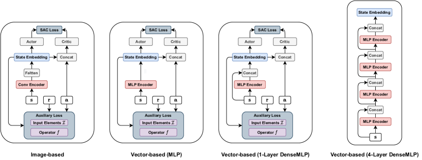
Figure 8: Network structures of image-based RL and vector-based RL with auxiliary losses.

C.1.2 Siamese Network

For a fair comparison with baseline methods, we follow the same Siamese network structure for representation learning as CURL [23]. As shown in Figure 2, when computing targets $\hat{y}$ for auxiliary losses, we map states to state embeddings with a target encoder. We stop gradients from target encoder $\hat{\theta}$ and update $\hat{\theta}$ in the exponential moving averaged (EMA) manner where $\hat{\theta}^{\prime}=\tau\theta+(1-\tau)\hat{\theta}$. This step, i.e., to freeze the gradients of the target encoder, is necessary when the loss is computed without negative samples. Otherwise, encoders will collapse to generate the same representation for any input. We have verified this in our early experiments.

C.2 Loss Operators

Instance Discrimination

Our implementation is based on InfoNCE loss [33]:

$$L=\log\frac{\exp(\phi(y,\hat{y}))}{\exp(\phi(y,\hat{y}))+\sum_{i=0}^{K-1}\exp(\phi(y,y_{i}))}$$ (8)

The instance discrimination loss can be interpreted as a log-loss of a K-way softmax classifier whose label is $\hat{y}$. The difference between discrimination-based loss operators lies in the discrimination objective $\phi$ used to measure agreement between $(y,\hat{y})$ pairs. Inner employs inner product $\phi(y,\hat{y})=y^{\top}\hat{y}$ while Bilinear employs bilinear product $\phi(y,\hat{y})=yW\hat{y}$, where $W$ is a learnable parameter matrix. Cosine uses cosine distance $\phi(y,\hat{y})=\frac{y^{\top}\hat{y}}{\|y\|\cdot\|\hat{y}\|}$ for further matrix calculation. As for losses implemented with cross entropy calculation without negative samples, we only take diagonal elements of matrix $M$ where $M_{i,j}=\phi(y_{j},\hat{y_{i}})$ for cross entropy calculation.

Mean Squared Error

The implementation of MSE-based loss operators are straightforward. MSE loss operator = $(y-\hat{y})^{2}$ while normalized MSE = $(\frac{y}{\|y\|}-\frac{\hat{y}}{\|\hat{y}\|})^{2}$. When combined with negative samples, MSE loss operator (with negative pairs) = $(y-\hat{y})^{2}-(y-y_{i})^{2}$ while normalized MSE (with negative pairs) = $(\frac{y}{\|y\|}-\frac{\hat{y}}{\|\hat{y}\|})^{2}-(\frac{y}{\|y\|}-\frac{y_{i}}{\|y_{i}\|})^{2}$.

C.3 Evolution Strategy

Horizon-changing Mutations

There are two kinds of mutations that can change horizon length. One is to decrease horizon length. Specifically, we remove the last time step, i.e., $(s_{t+k},a_{t+k},r_{t+k})$ if the target horizon length is $k$. The other is to increase horizon length, in which we append three randomly generated bits to the given masks at the end. We do not shorten the horizon when it becomes too small (less than 1) or lengthen the horizon when it is too long (exceeding 10).

Mutating Source and Target Masks

When mutating a candidate, the mutation on the source and the target are independent except for horizon change mutation where two masks should either both increase horizon or decrease horizon.

Initialization

At each initialization, we randomly generate 75 auxiliary loss functions (every bit of masks are generated from $\text{Bernoulli}(p)$ where $p=0.5$.) and generate 25 auxiliary loss functions with prior probability, which makes the auxiliary loss have some features like forward dynamics prediction or reward prediction. The prior probability for generating the pattern of forward dynamics prediction is: (i) every bit of states from target is generated from $\text{Bernoulli}(p)$ where $p=0.2$; (ii) every bit of actions from source is generated from $\text{Bernoulli}(p)$ where $p=0.8$; (iii) every bit of states from target is generated by flipping the states of source; (iv) The other bits are generated from $\text{Bernoulli}(p)$ where $p=0.5$. The prior probability for generating the pattern of reward prediction is: (i) every bit of rewards from target is generated from $\text{Bernoulli}(p)$ where $p=0.8$; (ii) Every bit of states and actions from target is 0; (iii) The other bits are generated from $\text{Bernoulli}(p)$ where $p=0.5$.

C.4 Training Details

C.4.1 Hyper-parameters in the Image-based Setting

We use the same hyper-parameters for A2LS, SAC-wo-aug, SAC and CURL during the search phase to ensure a fair comparison. When evaluating the searched auxiliary loss, we use a slightly larger setting (e.g., larger batch size) to train RL agents sufficiently. A full list is shown in Table 6.

Table 6: Hyper-parameters used in image-based environments.

Hyper-parameter	During Evolution	Final Evaluation of A2-winner
Random crop	False for SAC-wo-aug; True for others	True
Observation rendering	(84, 84) for SAC-wo-aug; (100, 100) for others	(100, 100)
Observation downsampling	(84, 84)	(84, 84)
Replay buffer size	100000	100000
Initial steps	1000	1000
Stacked frames	3	3
Actoin repeat	4 (Cheetah-Run, Reacher-Easy) 2 (Walker-Walk);	8 (Cartpole-Swingup); 4 (Others) 2 (Walker-Walk, Finger-Spin)
Hidden units (MLP)	1024	1024
Hidden units (Predictor MLP)	256	256
Evaluation episodes	10	10
Optimizer	Adam	Adam
($\beta_{1},\beta_{2}$) for actor/critic/encoder	(.9, .999)	(.9, .999)
($\beta_{1},\beta_{2}$) for entropy $\alpha$	(.5, .999)	(.5, .999)
Learning rate for actor/critic	1e-3	2e-4 (Cheetah-Run); 1e-3 (Others)
Learning rate for encoder	1e-3	3e-3 (Cheetah-Run, Finger-Spin, Walker-Walk); 1e-3 (Others)
Learning for $\alpha$	1e-4	1e-4
Batch size for RL loss	128	512
Batch size for auxiliary loss	128	128 (Walker-Walk) 256 (Cheetah-Run, Finger-Spin) 512 (Others);
Auxiliary Loss multipilier $\lambda$	1	1
Q function EMA $\tau$	0.01	0.01
Critic target update freq	2	2
Convolutional layers	4	4
Number of filters	32	32
Non-linearity	ReLU	ReLU
Encoder EMA $\tau$	0.05	0.05
Latent dimension	50	50
Discount $\gamma$	.99	.99
Initial temperature	0.1	0.1

C.4.2 Hyper-parameters in the Vector-based Setting

We use the same hyper-parameters for A2LS, SAC-Identity, SAC-DenseMLP and CURL-DenseMLP, shown in Table 7. Since training in vector-based environments is substantially faster than in image-based environments, there is no need to balance training cost and agent performance. We use this setting for both the search and final evaluation phases.

Table 7: Hyper-parameters used in vector-based environments.

Replay buffer size	100000
Initial steps	1000
Action repeat	4
Hidden units (MLP)	1024
Hidden units (Predictor MLP)	256
Evaluation episodes	10
Optimizer	Adam
($\beta_{1},\beta_{2}$) for actor/critic/encoder	(.9, .999)
($\beta_{1},\beta_{2}$) for entropy $\alpha$	(.5, .999)
Learning rate for actor/critic/encoder	2e-4 (Cheetah-Run); 1e-3 (Others)
Learning for $\alpha$	1e-4
Batch size	512
Auxiliary Loss multipilier $\lambda$	1
Q function EMA $\tau$	0.01
Critic target update freq	2
DenseMLP Layers	1
Non-linearity	ReLU
Encoder EMA $\tau$	0.05
Latent dimension of DenseMLP	40
Discount $\gamma$	.99
Initial temperature	0.1

C.5 Baselines Implementation

Image-based Setting

These following baselines are chosen because they are competitive methods for benchmarking control from pixels. CURL [23] is the main baseline to compare within the image-based setting, which is considered to be the state-of-the-art image-based RL algorithm. CURL learns state representations with a contrastive auxiliary loss. PlaNet [16] and Dreamer [15] are model-based methods that generate synthetic rollouts with a learned world model. SAC+AE [51] uses a reconstruction auxiliary loss of images to boost RL training. SLAC [26] leverages forward dynamics to construct a latent space for RL agents. Note that there are two versions of SLAC with different gradient Updates per agent step: SLACv1 (1:1) and SLACv2(3:1). We adopt SLACv1 for comparison since all methods only make one gradient update per agent step. Image SAC is just vanilla SAC [14] agents with images as inputs.

Vector-based Setting

As for the vector-based setting, we compare A2LS with SAC-Identity, SAC and CURL. SAC-Identity is the vanilla vector-based SAC where states are directly fed to actor/critic networks. SAC and CURL use the same architecture of 1-layer densely connected MLP as a state encoder. Note that both A2LS and baseline methods use the same hyper-parameter reported in Table 7 without additional hyper-parameter tuning.

Appendix D Additional Experiment Results

D.1 Search Space Pruning

Results of Search Space Pruning

Considering that the loss space is huge, an effective optimization strategy is required. Directly grid-searching over the whole space is infeasible because of unacceptable computational costs. Thus some advanced techniques such as space pruning and an elaborate search strategy are necessary. Our search space can be seen as a combination of the space for the input $\mathcal{I}$ and the space for the operator $f$. Inspired by AutoML works [5, 52] that search for hyper-parameters first and then neural architectures, we approximate the joint search of input and operator in Equation 1 in a two-step manner. The optimal auxiliary loss $\{\mathcal{I}^{*},f^{*}\}$ can be optimized as:

$$\begin{split}\max_{\mathcal{L}}\mathcal{R}(M_{\omega^{*}(\mathcal{L})};\mathcal{E})&=\max_{\mathcal{I},f}\mathcal{R}(M_{\omega^{*}(\mathcal{I},f)};\mathcal{E})\approx\max_{\mathcal{I}}\mathcal{R}(M_{\omega^{*}(\mathcal{I},f^{*})};\mathcal{E})\\ \text{where}\quad f^{*}&\approx\operatorname*{arg\,max}_{f}\mathbb{E}_{\mathcal{I}}[\mathcal{R}(M_{\omega^{*}(\mathcal{I},f)};\mathcal{E})]\end{split}$$ (9)

To decide the best loss operator, for every $f$ in the operator space, we estimate $\mathbb{E}_{\mathcal{I}}[\mathcal{R}(M_{\omega^{*}(\mathcal{I},f)};\mathcal{E})]$ with a random sampling strategy. We run 15 trials for each loss operator to estimate performance expectation. For each of 10 possible $f$ in the search space (5 operators with optional negative samples), we run 5 trials on each of the 3 image-based environments (used in evolution) with the same input elements $\{s_{t},a_{t}\}\rightarrow\{s_{t+1}\}$, as we found that forward dynamics is a reasonable representative of our search space with highly competitive performance. Surprisingly, as summarized in Table 8, the simplest MSE without negative samples outperforms all other loss operators with complex designs. Therefore, this loss operator is chosen for the rest of this paper.

Table 8: Normalized episodic rewards (mean & standard deviation for 5 seeds) of 3 environments used in evolution on image-based DMControl500K with different loss operators.

Loss operator and discrimination	Inner	Bilinear	Cosine	MSE	N-MSE
w/ negative samples	$0.979\pm 0.344$	$0.953\pm 0.329$	$0.872\pm 0.412$	$0.124\pm 0.125$	$0.933\pm 0.360$
w/o negative samples	$0.669\pm 0.311$	$0.707\pm 0.299$	$0.959\pm 0.225$	$\bf{1.000\pm 0.223}$	$0.993\pm 0.229$

Ablation Study on Search Space Pruning

As introduced in Section D.1, we decompose the full search space into operator and input elements. Here we try to directly apply the evolution strategy to the whole space without the pruning step. The comparison results are shown in Figure 9. We can see that pruning improves the evolution process, making it easier to find good candidates.

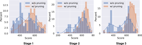
Figure 9: Comparison of evolution with and without pruning by performance histogram.

D.2 Learning Curves for A2LS on Image-based DMControl

We benchmark the performance of A2LS to the best-performing image-based baseline (CURL). As shown in Figure 10, the sample efficiency of A2LS outperforms CURL in 10 out of 12 environments. Note that the learning curves of CURL may not match the data in Table 2. This is because we use the data reported in the CURL paper for tabular while we rerun CURL for learning curves plotting, where we find the performance of our rerunning CURL is sightly below the CURL paper.

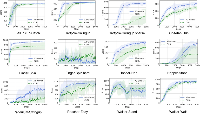
Figure 10: Learning curves of A2-winner and CURL on 12 DMC environments. Shadow represents the standard deviation over five random seeds. The curves are uniformly smoothed for visual display. The y-axis represents episodic reward and x-axis represents interaction steps.

D.3 Effectiveness of AULC scores

To illustrate why we use the area under learning curve (AULC) instead of other metrics, we select top-10 candidates with different evolution metrics. In practice, AULC is calculated as the sum of scores of all checkpoints during training. Figure 11 demonstrates the usage of AULC score could well balance both sample efficiency and final performance. The learning curves of the top-10 candidates selected by AULC score look better than the other two metrics (that select top candidates simply with 100k step score or 500k step score).

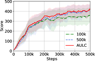
Figure 11: Learning curves of top-10 loss candidates selected with different metrics.

D.4 Comparing Auxiliary Loss with Data Augmentation

Besides auxiliary losses, data augmentation has been shown to be a strong technique for data-efficient RL, especially in image-based environments[25, 22]. RAD [25] can be seen as a version of CURL without contrastive loss but with a better image transformation function for data augmentation. We compare A2-winner with RAD in both image-based and vector-based DMControl environments. The learning curves in image-based environments are shown in Figure 12, where no statistically significant difference is observed. As readers may notice, the scores on RAD paper [25] are higher than the RAD and A2-winner learning curves reported. To avoid a misleading conclusion that RAD is much stronger than A2-winner , we would like to emphasize some key differences between RAD and our implementationt: 1) Large Conv encoder output dim (RAD: 47, A2LS/CURL: 25); 2) Larger image size (RAD: 108, A2LS/CURL: 100); 3) Larger encoder feature dim (RAD: 64, A2LS/CURL: 50). We use the hyper-parameters used in CURL for consistency of scores reported in our paper. However, in vector-based environments, as shown in Figure 13, A2-winner greatly outperforms RAD. Due to the huge difference between images and proprioceptive features, RAD could not transfer augmentation techniques like random crop and transforms used for images to vectors. Though RAD designs noise and random scaling for proprioceptive features, A2-winner shows much better performance on vector-based settings. These results show that recent progress in using data augmentation for RL is still limited to image-based RL while using auxiliary loss functions for RL is able to boost RL across environments with totally different data types of observation. Besides comparing auxiliary losses with data augmentation in DMC, we also provide experimental results in Atari [1]. As shown in Table 3, A2-winner significantly outperforms DrQ [22].

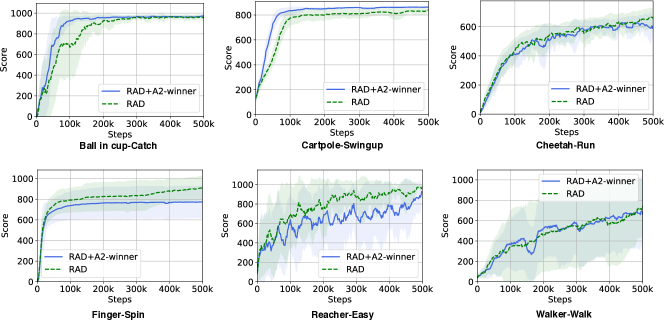
Figure 12: Comparison of learning curves of A2LS and RAD in image-based DMC environments.

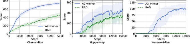
Figure 13: Comparison of learning curves of A2LS and RAD in vector-based DMControl environments.

D.5 Evolution on Vector-based RL

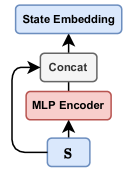
Figure 14: Network architecture of 1-layer DenseMLP state encoder.

Experiment Settings

As for vector-based RL, we use a 1-layer densely connected MLP as the state encoder as shown in Figure 14 due to the low-dimensional state space. So, for this setting, we focus on this simple encoder structure. Additional ablations on state encoder architectures are given in Section D.6. In the search phase, we compare A2LS to SAC-Identity, SAC-DenseMLP, CURL-DenseMLP. To ensure a fair comparison, all SAC related hyper-parameters are the same as those reported in the CURL paper. Details can be found in Section C.4.2. SAC-Identity is vanilla SAC with no state encoder, while the other three methods (A2LS, SAC-DenseMLP, CURL-DenseMLP) use the same encoder architecture. Different from the image-based setting, there is no data augmentation in the vector-based setting. Note that many environments that are challenging in image-based settings become easy to tackle with vector-based inputs. Therefore we apply our search framework to more challenging environments for vector-based RL, including Cheetah-Run, Hopper-Hop and Quadruped-Run.

Search Results

Similar to image-based settings, we approximate AULC with the average score agents achieved at 300k, 600k, 900k, 1200k, and 1500k time steps. For each environment, we early stop the experiment when the budget of 1,500 GPU hours is exhausted. The evolution process is shown in Figure 15, where we find a large portion of candidates outperform baselines (horizontal dashed lines). The performance improvement is especially significant on Cheetah-Run, where almost all candidates in the population greatly outperform all baselines by the end of the first stage. Similar to image-based settings, we also use cross-validation to select the best loss function, which we call “A2-winner-v” here (all the top candidates during evolution are reported in Appendix F)

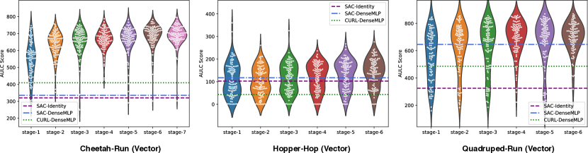
Figure 15: Evolution process in in the three training (vector-based) environments. Every white dot represents a loss candidate, and the score of y-axis shows its corresponding approximated AULC score. The horizontal lines show the scores of baselines. The AULC score is approximated with the average evaluation score at 300k, 600k, 900k, 1200k, 1500k time steps (Cheetah-Run at 100k, 200k, 300k, 400K).

D.6 Encoder Architecture Ablation for Vector-based RL

Table 9: Normalized episodic rewards of A2LS (mean & standard deviation for 5 seeds of 6 environments) on v DMControl100K with different encoder architectures.

A2LS-MLP (1-layer)	A2LS-MLP (4-layer)	A2LS-DenseMLP (1-layer)	A2LS-DenseMLP (4-layer)
0.919 $\pm$ 0.217	0.544 $\pm$ 0.360	1.000 $\pm$ 0.129	0.813 $\pm$ 0.218

As shown in Figure 14, we choose a 1-layer densely connected MLP as the state encoder for vector-based RL. We conduct an ablation study on different encoder architectures in the vector-based setting. The results are summarized in Table 9, where A2LS with 4-layer encoders consistently perform worse than 1-layer encoders. We also note that dense connection is helpful in the vector-based setting compared with naive MLP encoders.

D.7 Visualization of Loss Landscape

In an effort to reveal why auxiliary losses are helpful to RL, we draw the loss landscape of critic loss of both A2-winner and SAC using the technique in [29, 34]. We choose Humanoid-Stand as the testing environment since we observe the most significant advantage of A2-winner over SAC on complex robotics tasks like Humanoid. Note that the only difference between A2-winner and SAC is whether using auxiliary loss or not. As shown in Figure 16, the critic loss landscape of A2-winner appears to be convex during training, while the loss landscape of SAC becomes more non-convex as training proceeds. The auxiliary loss of A2-winner is able to efficiently boost Q learning (gaining near 300 reward at 500k steps), while SAC suffers from the poor results of critic learning (gaining near 0 reward even at 1000k time steps). This result shows that such an auxiliary loss might make learning easier from an optimization perspective.

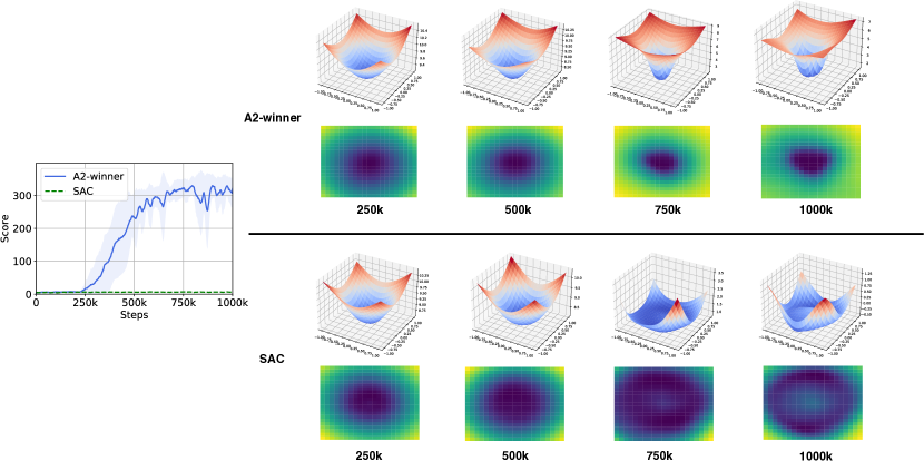
Figure 16: Left: Learning curves of A2-winner and SAC on vector-based Humanoid-Stand. Right: Critic Loss Landscape of A2-winner (upper right ) and SAC (lower right) at 250k, 500k, 750k and 1000k time steps, trained on vector-based Humanoid-Stand. The first row shows 3D surface plots, and the second row shows heatmap plots of loss landscapes.

D.8 Histogram of Auxiliary Loss Analysis

The histogram of each pattern analysis is shown in Figure 17.

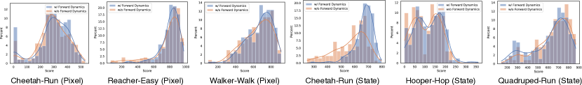
(a) Forward dynamics

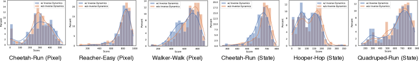
(b) Inverse dynamics

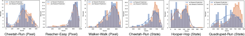
(c) Reward prediction

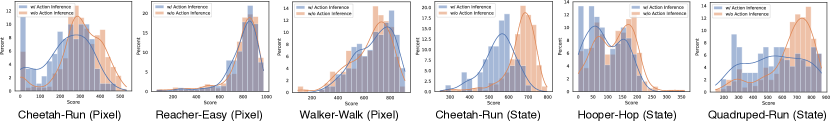
(d) Action inference

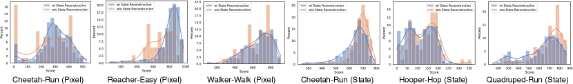
(e) State reconstruction

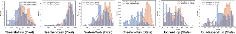
(f) State source & target

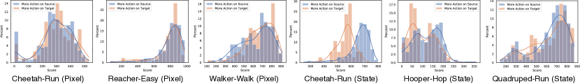
(g) Action source & target

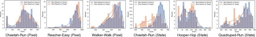
(h) Reward source & target

Figure 17: Histogram of statistical analysis of auxiliary loss candidates in six evolution processes. The x-axis represents approximated AULC score while the y-axis represents the percentage of the corresponding bin of population. Best viewed in color.

D.9 Comparing A2-winner with Advanced Human-designed Auxiliary Losses

Besides CURL, many recent works (e.g., SPR [39] and ATC [42]) also proposed advanced auxiliary losses that achieve strong performance. Surprisingly, we find that both SPR and ATC designed similar patterns as we conclude in Section 6, like forward dynamics and $n_{\text{target}}>n_{\text{source}}$. Particularly, in ATC, they train the encoder only with ATC loss, and we find the performance of A2-winner has better performances than the results reported in their paper: we are 2$\times$ more sample efficient to reach 800 scores on Cartpole-Swingup, 2$\times$ more sample efficient to reach 100 scores on Hopper-Hop, and 3$\times$ more sample efficient to reach 600 scores on Cartpole-Swingup sparse (see Figure 2 of [42]). As for SPR, we find they have superior performance on Atari games benchmark, as shown in Table 10, where A2-winner outperform all baselines except SPR. However, note that, our A2-winner is only searched on a small set of DMC benchmarks and can still generalize well to discrete-control tasks of Atari, while SPR is designed and only evaluated on Atari environments. In addition, we believe such a gap can arise from different base RL algorithm implementation (A2LS is based on Efficient Rainbow DQN while SPR adopts Categorical DQN) and different hyper-parameters.

Table 10: Mean and Median scores (normalized by human score and random score) achieved by A2LS and baselines on 26 Atari games benchmarked at 100k time-steps (Atari100k).

Metric	A2-winner	CURL	Eff. Rainbow	DrQ [22]	SimPLe	DER	OTRainbow	SPR	Random	Human
Mean Human-Norm’d	0.568	0.381	0.285	0.357	0.443	0.285	0.264	0.704	0.000	1.000
Median Human-Norm’d	0.317	0.175	0.161	0.268	0.144	0.161	0.204	0.415	0.000	1.000

D.10 The Trend of Increasing Performance during Evolution

Table 11: Average AULC scores of populations of each stage.

	stage-1	stage-2	stage-3	stage-4	stage-5	stage-6	stage-7	SAC (baseline)
Cheetah-Run	191.75	252.51	258.09	284.53	349.52	351.51	352.57	285.82
Reacher-Easy	674.87	782.75	812.61	823.04	810.15	811.88	827.19	637.60
Walker-Walk	599.38	633.75	716.18	702.49	N/A	N/A	N/A	675.84

Table 12: Average AULC scores of Top-5 candidates of each stage.

	stage-1	stage-2	stage-3	stage-4	stage-5	stage-6	stage-7	SAC (baseline)
Cheetah-Run	398.18	424.27	428.08	485.54	487.94	482.65	498.46	285.82
Reacher-Easy	931.27	950.61	943.83	938.91	954.77	955.02	969.43	637.60
Walker-Walk	834.09	883.77	896.52	880.73	N/A	N/A	N/A	675.84

To illustrate the trend of increasing performance during evolution, we provide the average AULC score of populations of each stage in Table 11. As for comparing evoluationary search with random sampling, we can take the stage-1 of each evolution procedure as random sampling. As shown in Table 11, the average performance of the stage-1 population (i.e., random sampling) is even worse than SAC in Cheetah-Run and Walker-Walk. Nevertheless, as evolution continues, the performance of the evolved population in the following stages improves significantly, surpassing the score of SAC.

To illustrate the trend of increasing performance of best individuals during evolution, we provide the average AULC score of the top 5 candidates of the population at each stage in Table 12. As shown in Table 12, there is an obvious trend that the performance of the best individuals in the population at each stage continues to improve and also outperformed the baseline by a large margin during the evolution across all the three training environments.

Appendix E Search Space Complexity Analysis

The search space size is calculated by the size of input element space multiplying by the size of the loss operator space.

For input elements, the search space for input elements is a pair of binary masks $(m,\hat{m})$, each of which is up to length $(3k+3)$ if the length of an interaction data sequence, i.e., horizon, is limited to $k$ steps. In our case, we set the maximum horizon length $k_{\text{max}}=10$. we calculate separately for each possible horizon length $k$. When length is $k$, the interaction sequence length $(s_{t},a_{t},r_{t},\cdots,s_{t+k})$ has length $(3k+3)$. For binary mask $\hat{m}$, there are $2^{3k+3}$ different options. There are also $2^{3k+3}$ distinct binary mask $m$ to select targets. Therefore, there are $2^{6k+6}$ combinations when horizon length is fixed to $k$. As our maximum horizon is 10, we enumerate $k$ from $1$ to $10$, resulting in $\sum_{i=1}^{10}2^{6i+6}$.

For operator, we can learn intuitively from Table 8 that there are 5 different similarity measures with or without negative samples, resulting in $5\times 2=10$ different loss operators.

In total, the size of the entire space is

$$10\times\sum_{i=1}^{10}2^{6i+6}\approx 7.5\times 10^{20}.$$

Appendix F Top-performing Auxiliary Losses

F.1 A2-winner and A2-winner-v

We introduce all the top-performing auxiliary losses during evolution in this section. Note that MSE is chosen (details are given Section D.1) as the loss operator for all the auxliary losses reported below. The source $\text{seq}_{source}$ and target $\text{seq}_{target}$ of auxiliary loss of A2-winner are:

$$\{s_{t+1},a_{t+1},a_{t+2},a_{t+3}\}\rightarrow\{r_{t},r_{t+1},s_{t+2},s_{t+3}\},$$ (10)

where A2-winner is the third-best candidate of stage 4 in Cheetah-Run (Image).

The source $\text{seq}_{source}$ and target $\text{seq}_{target}$ of auxiliary loss of A2-winner-v are:

$$\begin{split}\{s_{t},a_{t},a_{t+1},s_{t+2},a_{t+2},a_{t+3},r_{t+3},a_{t+4},r_{t+4},a_{t+5},a_{t+7},s_{t+8},a_{t+8},r_{t+8}\}\\ \rightarrow\{s_{t+1},s_{t+3},a_{t+4},s_{t+6},s_{t+9}\},\end{split}$$ (11)

where A2-winner-v is the fourth-best candidate of stage 4 in Cheetah-Run (Vector).

These two losses are chosen because they are the best-performing loss functions during cross-validation.

F.2 During Evolution

We report all the top-5 auxiliary loss candidates during evolution in this section.

Table 13: Top-5 candidates of each stage in Cheetah-Run (Image) evolution process

Cheetah-Run (Image)
Stage-1	$\{r_{t},s_{t+1},a_{t+1},r_{t+1},a_{t+2},r_{t+2},a_{t+3},r_{t+3}\}\rightarrow\{s_{t},a_{t},s_{t+2},s_{t+3},s_{t+4}\}$ $\{s_{t},a_{t},r_{t}\}\rightarrow\{s_{t+1}\}$ $\{s_{t},a_{t},a_{t+1},r_{t+2}\}\rightarrow\{s_{t},a_{t},s_{t+1},a_{t+1},r_{t+1},s_{t+2},r_{t+2},s_{t+3}\}$ $\{s_{t},r_{t},a_{t+1},a_{t+2},a_{t+3},r_{t+3},r_{t+4},a_{t+5},r_{t+5},s_{t+6},s_{t+7}\}\rightarrow\{s_{t},a_{t},s_{t+1},s_{t+2},r_{t+2},r_{t+3},s_{t+4},r_{t+5},s_{t+6},a_{t+6},s_{t+7}\}$ $\{s_{t},a_{t},s_{t+1},a_{t+1},s_{t+2},r_{t+2}\}\rightarrow\{s_{t},s_{t+1},r_{t+1},s_{t+2},r_{t+2},s_{t+3}\}$
Stage-2	$\{s_{t},a_{t+1},r_{t+2},s_{t+4},r_{t+4}\}\rightarrow\{s_{t+2},a_{t+3},r_{t+3},a_{t+4},s_{t+5}\}$ $\{s_{t},a_{t},a_{t+2},r_{t+2}\}\rightarrow\{s_{t},r_{t},s_{t+1},s_{t+2},r_{t+2}\}$ $\{a_{t},r_{t},s_{t+1},r_{t+1},s_{t+2},a_{t+2},r_{t+2},a_{t+3},a_{t+4}\}\rightarrow\{s_{t+1},s_{t+2},s_{t+3},a_{t+3},s_{t+4}\}$ $\{s_{t},a_{t},r_{t},a_{t+1},r_{t+1},a_{t+2},r_{t+2},a_{t+3},a_{t+4}\}\rightarrow\{s_{t},s_{t+1},s_{t+2},s_{t+4},s_{t+5}\}$ $\{r_{t},s_{t+1},r_{t+1}\}\rightarrow\{s_{t},a_{t},a_{t+1},s_{t+2}\}$
Stage-3	$\{s_{t},a_{t},a_{t+2},r_{t+2}\}\rightarrow\{s_{t},s_{t+1},s_{t+2},r_{t+2}\}$ $\{s_{t},r_{t},a_{t+1},a_{t+3},r_{t+3},r_{t+4},a_{t+5},r_{t+5},s_{t+6},a_{t+6},s_{t+7}\}\rightarrow\{s_{t},a_{t},s_{t+1},s_{t+2},r_{t+2},r_{t+3},s_{t+4},r_{t+5},s_{t+6},s_{t+7},a_{t+7}\}$ $\{s_{t},a_{t},a_{t+1},r_{t+1},a_{t+2},r_{t+2},a_{t+3},s_{t+4},a_{t+4}\}\rightarrow\{s_{t+1},s_{t+2},s_{t+4},s_{t+5}\}$ $\{s_{t},a_{t},a_{t+1},r_{t+1},r_{t+2},s_{t+3},a_{t+3},r_{t+4}\}\rightarrow\{s_{t+1},s_{t+2},r_{t+3},s_{t+4},a_{t+4},s_{t+5}\}$ $\{r_{t},s_{t+1}\}\rightarrow\{s_{t},a_{t},a_{t+1},s_{t+2}\}$
Stage-4	$\{s_{t},s_{t+1},a_{t+2},r_{t+2},s_{t+3},s_{t+4}\}\rightarrow\{a_{t+1},s_{t+2},r_{t+2},s_{t+4},a_{t+4},s_{t+5}\}$ $\{s_{t},a_{t},a_{t+1},r_{t+1},r_{t+2},s_{t+3},a_{t+3}\}\rightarrow\{s_{t+1},s_{t+2},r_{t+3},s_{t+4}\}$ $\{s_{t}\}\rightarrow\{s_{t},r_{t},s_{t+1},r_{t+1},s_{t+2},a_{t+2},r_{t+2}\}$ $\{s_{t},r_{t},a_{t+1},s_{t+2},a_{t+2},r_{t+2},a_{t+3},r_{t+3},a_{t+4}\}\rightarrow\{s_{t},a_{t},s_{t+1},r_{t+1},r_{t+3},s_{t+4},a_{t+4},s_{t+5}\}$ $\{r_{t},s_{t+1},a_{t+1}\}\rightarrow\{s_{t},a_{t},a_{t+1},s_{t+2}\}$
Stage-5∗	$\{a_{t},r_{t},s_{t+1},a_{t+1},r_{t+1},a_{t+2},r_{t+2},a_{t+3},r_{t+3}\}\rightarrow\{r_{t},s_{t+1},a_{t+1},s_{t+2},s_{t+4}\}$ $\{s_{t},a_{t+1},r_{t+2},a_{t+3},s_{t+4},r_{t+4}\}\rightarrow\{s_{t+1},s_{t+2},a_{t+3},s_{t+4},a_{t+4},s_{t+5}\}$ ${}^{\dagger}\{s_{t+1},a_{t+1},a_{t+2},a_{t+3}\}\rightarrow\{r_{t},r_{t+1},s_{t+2},s_{t+3}\}$ $\{s_{t}\}\rightarrow\{s_{t},r_{t},s_{t+1},r_{t+1},s_{t+2}\}$ $\{s_{t}\}\rightarrow\{s_{t},r_{t},s_{t+1},r_{t+1},s_{t+2},r_{t+2}\}$
Stage-6	$\{a_{t+1},r_{t+1},s_{t+2},r_{t+2},a_{t+3},a_{t+4}\}\rightarrow\{r_{t},s_{t+1},r_{t+1},r_{t+3},s_{t+4},a_{t+4},s_{t+5}\}$ $\{s_{t},a_{t+1},a_{t+3},s_{t+4},r_{t+4}\}\rightarrow\{s_{t+1},s_{t+2},a_{t+3},s_{t+4},a_{t+4},s_{t+5}\}$ $\{s_{t},a_{t+1},r_{t+1},s_{t+2},a_{t+2},r_{t+2},s_{t+3},a_{t+3},r_{t+3}\}\rightarrow\{a_{t},s_{t+2},r_{t+2},a_{t+3},s_{t+4},a_{t+4},s_{t+5}\}$ $\{s_{t},a_{t+1},r_{t+2},a_{t+3},s_{t+4},r_{t+4}\}\rightarrow\{s_{t+1},s_{t+2},a_{t+3},s_{t+4},a_{t+4},s_{t+5},a_{t+5}\}$ $\{s_{t},a_{t+1},a_{t+2},r_{t+2},s_{t+3},a_{t+3},s_{t+4},r_{t+4}\}\rightarrow\{s_{t+1},a_{t+1},s_{t+2},r_{t+2},s_{t+4},a_{t+4},r_{t+4},s_{t+5}\}$
Stage-7	$\{s_{t},a_{t},r_{t},a_{t+1},r_{t+2},a_{t+3},s_{t+4}\}\rightarrow\{a_{t},r_{t},s_{t+2},r_{t+3},s_{t+4},a_{t+4},r_{t+4},s_{t+5}\}$ $\{s_{t},r_{t+2},a_{t+3},s_{t+4}\}\rightarrow\{a_{t},s_{t+1},s_{t+2},r_{t+2},a_{t+3},r_{t+3},s_{t+4},a_{t+4},r_{t+4},s_{t+5}\}$ $\{s_{t+1},a_{t+2},r_{t+2},s_{t+3},a_{t+3},r_{t+3},s_{t+4}\}\rightarrow\{r_{t},a_{t+1},r_{t+1},s_{t+2},r_{t+2},s_{t+4},a_{t+4},s_{t+5}\}$ $\{s_{t},a_{t+1},s_{t+2},a_{t+2},r_{t+2},s_{t+3},a_{t+3},r_{t+3},a_{t+4}\}\rightarrow\{a_{t},s_{t+1},s_{t+2},r_{t+2},s_{t+3},r_{t+3},s_{t+4},a_{t+4},s_{t+5}\}$ $\{s_{t},a_{t+1},r_{t+2},a_{t+3},s_{t+4},r_{t+4}\}\rightarrow\{s_{t+1},s_{t+2},r_{t+2},a_{t+3},s_{t+4},a_{t+4},s_{t+5},a_{t+5}\}$

• $*$: Used for cross-validation. ${\dagger}$: A2-winner.

Table 14: Top-5 candidates of each stage in Reacher-Easy (Image) evolution process

Reacher-Easy (Image)
Stage-1	$\{s_{t+1},a_{t+1}\}\rightarrow\{r_{t},r_{t+1}\}$ $\{r_{t},s_{t+1},a_{t+1},s_{t+2},a_{t+2},r_{t+2},a_{t+3},a_{t+4},r_{t+4},s_{t+5},a_{t+5},r_{t+5},s_{t+6},a_{t+6},r_{t+6},r_{t+7},s_{t+8},a_{t+8},s_{t+9}\}\rightarrow\{a_{t+1},r_{t+1},s_{t+2},s_{t+3},r_{t+3},s_{t+4},a_{t+4},a_{t+5},a_{t+6},r_{t+6},s_{t+7},a_{t+7},r_{t+7},a_{t+8},r_{t+8},s_{t+10}\}$ $\{s_{t},r_{t},s_{t+1},a_{t+2},s_{t+4},a_{t+4},r_{t+5},s_{t+6},a_{t+6},a_{t+7},s_{t+9},s_{t+10}\}\rightarrow\{s_{t},s_{t+1},r_{t+1},s_{t+2},r_{t+2},r_{t+3},s_{t+4},a_{t+4},r_{t+4},s_{t+5},s_{t+6},a_{t+6},r_{t+7},r_{t+8},s_{t+10}\}$ $\{s_{t},r_{t},s_{t+1},a_{t+1},s_{t+2},s_{t+3},a_{t+3},a_{t+4},s_{t+5},r_{t+5},a_{t+6},r_{t+6},s_{t+7}\}\rightarrow\{a_{t+1},s_{t+2},a_{t+2},r_{t+2},s_{t+3},a_{t+3},r_{t+3},s_{t+4},a_{t+4},r_{t+4},s_{t+6},a_{t+6}\}$ $\{s_{t+1},r_{t+1},a_{t+2},r_{t+2},r_{t+3},s_{t+4},a_{t+4},r_{t+4},s_{t+5},s_{t+6},r_{t+6}\}\rightarrow\{r_{t},s_{t+1},s_{t+2},a_{t+2},r_{t+2},s_{t+4},s_{t+5},r_{t+5},s_{t+6},a_{t+6},s_{t+7},s_{t+8}\}$
Stage-2	$\{s_{t},s_{t+1},a_{t+1}\}\rightarrow\{r_{t},r_{t+1}\}$ $\{s_{t},r_{t},a_{t+2},a_{t+3},s_{t+4},a_{t+4},r_{t+4},a_{t+5},r_{t+5},s_{t+6},a_{t+7},a_{t+8}\}\rightarrow\{r_{t},a_{t+1},s_{t+2},r_{t+2},s_{t+3},a_{t+3},r_{t+3},a_{t+4},r_{t+4},a_{t+5},r_{t+5},a_{t+6},s_{t+7},s_{t+9}\}$ $\{s_{t},a_{t},r_{t},s_{t+1},a_{t+2},a_{t+3},s_{t+5}\}\rightarrow\{a_{t},s_{t+2},a_{t+2},r_{t+2},s_{t+3},a_{t+3},a_{t+4},r_{t+4}\}$ $\{s_{t},a_{t},s_{t+1},a_{t+3},s_{t+4},a_{t+4},a_{t+5},s_{t+6},a_{t+6},a_{t+7},r_{t+7},s_{t+9},a_{t+9}\}\rightarrow\{s_{t},a_{t},r_{t},s_{t+1},r_{t+1},s_{t+2},r_{t+3},s_{t+4},r_{t+4},s_{t+6},a_{t+6},r_{t+7},a_{t+8},s_{t+10}\}$ $\{s_{t},a_{t},r_{t},a_{t+1},a_{t+3},r_{t+3},s_{t+4},a_{t+4},s_{t+5},a_{t+5},r_{t+5},a_{t+6},r_{t+6},a_{t+7}\}\rightarrow\{s_{t+1},s_{t+2},a_{t+2},s_{t+3},s_{t+6},a_{t+6},s_{t+7},s_{t+8}\}$
Stage-3	$\{a_{t},s_{t+1},a_{t+1},s_{t+2},a_{t+2}\}\rightarrow\{r_{t},a_{t+1},r_{t+1},r_{t+2}\}$ $\{s_{t},a_{t},s_{t+1},s_{t+2},a_{t+2},a_{t+3},s_{t+4},r_{t+4},a_{t+5},r_{t+5},r_{t+6},a_{t+7}\}\rightarrow\{s_{t},a_{t},r_{t},s_{t+2},s_{t+3},a_{t+3},s_{t+4},a_{t+4},a_{t+5},r_{t+5},s_{t+6},s_{t+7},s_{t+8}\}$ $\{s_{t},a_{t},s_{t+1},a_{t+1},r_{t+1},s_{t+2},a_{t+2},a_{t+3},s_{t+4},r_{t+6},a_{t+7}\}\rightarrow\{r_{t},a_{t+2},r_{t+2},a_{t+3},r_{t+3},s_{t+4},a_{t+4},a_{t+5},s_{t+6},a_{t+6},s_{t+7},r_{t+7},s_{t+8}\}$ $\{s_{t},a_{t},s_{t+1},r_{t+1},a_{t+2},a_{t+3},s_{t+4},r_{t+4},s_{t+6},r_{t+6},a_{t+7}\}\rightarrow\{s_{t},r_{t},r_{t+1},a_{t+2},r_{t+2},a_{t+3},r_{t+3},s_{t+4},a_{t+4},a_{t+5},r_{t+5},s_{t+6},s_{t+7},s_{t+8}\}$ $\{s_{t},a_{t},r_{t},a_{t+1},r_{t+1},a_{t+2},s_{t+6},s_{t+7},a_{t+7},s_{t+8}\}\rightarrow\{s_{t},r_{t},s_{t+2},a_{t+2},r_{t+2},a_{t+3},r_{t+3},s_{t+8},a_{t+8}\}$
Stage-4	$\{s_{t},a_{t},r_{t},a_{t+1},a_{t+3},r_{t+3},s_{t+4},s_{t+5},a_{t+5},r_{t+5},a_{t+6},r_{t+6},a_{t+7}\}\rightarrow\{s_{t+1},s_{t+2},s_{t+3},r_{t+4},r_{t+5},r_{t+7},s_{t+8}\}$ $\{a_{t},s_{t+1},a_{t+1},s_{t+2}\}\rightarrow\{r_{t},r_{t+1},a_{t+2},r_{t+2}\}$ $\{s_{t},a_{t},r_{t},a_{t+1},r_{t+3},s_{t+4},s_{t+5},s_{t+6},r_{t+6},a_{t+7}\}\rightarrow\{s_{t+1},s_{t+2},a_{t+3},s_{t+4},r_{t+4},s_{t+5},s_{t+6},s_{t+7},r_{t+7},s_{t+8}\}$ $\{s_{t},a_{t},r_{t+1},a_{t+2},a_{t+3},s_{t+4},r_{t+4},r_{t+5},s_{t+6},r_{t+6},a_{t+7}\}\rightarrow\{s_{t},r_{t},r_{t+1},a_{t+2},r_{t+2},a_{t+3},r_{t+3},s_{t+4},a_{t+4},a_{t+5},r_{t+5},s_{t+6},s_{t+7},s_{t+8}\}$ $\{a_{t},s_{t+1},a_{t+1},s_{t+2},a_{t+2}\}\rightarrow\{r_{t},r_{t+1},r_{t+2}\}$
Stage-5	$\{s_{t},a_{t},a_{t+1},a_{t+2},a_{t+3},s_{t+4},s_{t+5},a_{t+6},r_{t+6},a_{t+7},s_{t+8}\}\rightarrow\{r_{t},a_{t+2},r_{t+2},a_{t+3},s_{t+4},s_{t+5},a_{t+5},s_{t+6},a_{t+6},s_{t+7},r_{t+7},s_{t+8}\}$ $\{s_{t},a_{t},s_{t+1},a_{t+1},r_{t+1}\}\rightarrow\{r_{t},s_{t+2}\}$ $\{s_{t},a_{t},r_{t},a_{t+1},r_{t+3},s_{t+4},s_{t+5},s_{t+6},r_{t+6},a_{t+7}\}\rightarrow\{s_{t+1},s_{t+2},a_{t+3},s_{t+4},r_{t+4},s_{t+5},r_{t+6},s_{t+7},r_{t+7},s_{t+8}\}$ $\{s_{t},a_{t},r_{t},a_{t+1},r_{t+1},s_{t+2},a_{t+2},a_{t+3},s_{t+4},s_{t+5},a_{t+5},r_{t+6},a_{t+7}\}\rightarrow\{s_{t},r_{t},a_{t+1},r_{t+1},a_{t+2},r_{t+2},s_{t+3},a_{t+3},s_{t+4},s_{t+6},a_{t+6},r_{t+6},s_{t+7}\}$ $\{s_{t},a_{t},s_{t+1},r_{t+1},a_{t+2},s_{t+3},s_{t+4},r_{t+6},a_{t+7},s_{t+8}\}\rightarrow\{s_{t},r_{t},r_{t+1},a_{t+2},r_{t+2},a_{t+3},s_{t+4},a_{t+4},a_{t+5},s_{t+6},r_{t+6},s_{t+7},s_{t+8}\}$
Stage-6	$\{s_{t},a_{t},r_{t},a_{t+1},a_{t+3},r_{t+3},s_{t+4},a_{t+4},s_{t+5},a_{t+5},r_{t+5},s_{t+6},a_{t+6},r_{t+6}\}\rightarrow\{s_{t+1},s_{t+2},a_{t+2},s_{t+3},r_{t+4},s_{t+6}\}$ $\{s_{t},a_{t},r_{t},s_{t+1},a_{t+1},r_{t+1},s_{t+2},a_{t+2},s_{t+3},a_{t+4},r_{t+5},r_{t+6},s_{t+7},s_{t+8}\}\rightarrow\{s_{t},r_{t},r_{t+2},a_{t+3},r_{t+3},s_{t+4},r_{t+4},a_{t+5},r_{t+5},s_{t+6},a_{t+6},r_{t+6},s_{t+7},a_{t+7},r_{t+7},s_{t+8}\}$ $\{s_{t},a_{t},r_{t},r_{t+1},a_{t+2},a_{t+3},s_{t+4},s_{t+5},r_{t+5}\}\rightarrow\{s_{t},r_{t},r_{t+1},a_{t+2},a_{t+3},r_{t+3},a_{t+4},r_{t+4},a_{t+5},s_{t+6},a_{t+6},r_{t+6},s_{t+7},s_{t+8}\}$ $\{s_{t},a_{t},s_{t+1},a_{t+3},a_{t+4},a_{t+5},s_{t+6},a_{t+6},s_{t+7},a_{t+7},r_{t+7},s_{t+9},a_{t+9}\}\rightarrow\{s_{t},a_{t},r_{t},s_{t+1},r_{t+1},s_{t+2},s_{t+3},r_{t+3},s_{t+4},a_{t+4},r_{t+4},s_{t+6},a_{t+6},r_{t+7},a_{t+8},a_{t+9},s_{t+10}\}$ $\{s_{t},a_{t},r_{t},a_{t+1},r_{t+1},a_{t+2},a_{t+3},s_{t+4},s_{t+5},a_{t+5},r_{t+6},a_{t+7}\}\rightarrow\{r_{t},s_{t+1},r_{t+1},a_{t+2},r_{t+2},s_{t+3},s_{t+4},s_{t+6},a_{t+6},r_{t+6},s_{t+7},s_{t+8}\}$
Stage-7	$\{s_{t},a_{t},s_{t+1},a_{t+1},r_{t+1},s_{t+2},a_{t+2},r_{t+5},r_{t+6},a_{t+7},s_{t+8}\}\rightarrow\{r_{t},a_{t+2},r_{t+2},r_{t+3},s_{t+4},a_{t+4},a_{t+5},a_{t+6},r_{t+6},s_{t+7},s_{t+8}\}$ $\{s_{t},a_{t},a_{t+1},s_{t+2},a_{t+2},a_{t+3},s_{t+4},a_{t+5},r_{t+5},r_{t+6},a_{t+7}\}\rightarrow\{s_{t+1},r_{t+2},a_{t+3},r_{t+3},s_{t+4},a_{t+5},r_{t+5},s_{t+6},a_{t+6},s_{t+7},r_{t+7}\}$ $\{s_{t},a_{t},r_{t},a_{t+2},a_{t+3},s_{t+4},s_{t+5},r_{t+5},a_{t+6}\}\rightarrow\{s_{t},r_{t},r_{t+1},s_{t+2},a_{t+2},a_{t+3},r_{t+3},r_{t+4},s_{t+6},s_{t+8}\}$ $\{s_{t},a_{t},r_{t},a_{t+1},a_{t+3},r_{t+3},s_{t+4},a_{t+4},s_{t+5},a_{t+5},r_{t+5},s_{t+6},a_{t+6},r_{t+6}\}\rightarrow\{r_{t},s_{t+1},s_{t+2},a_{t+2},s_{t+3},r_{t+4},s_{t+6}\}$ $\{s_{t},a_{t},r_{t},a_{t+1},r_{t+1},a_{t+3},r_{t+3},s_{t+4},a_{t+4},s_{t+5},r_{t+5},s_{t+6},a_{t+7},r_{t+7}\}\rightarrow\{s_{t},r_{t},s_{t+1},r_{t+1},a_{t+2},s_{t+3},a_{t+3},r_{t+4},s_{t+6},s_{t+8}\}$

Table 15: Top-5 candidates of each stage in Walker-Walk (Image) evolution process

Walker-Walk (Image)
Stage-1	$\{s_{t},a_{t},s_{t+2},a_{t+2},r_{t+2},s_{t+3},a_{t+4},a_{t+5},s_{t+6},a_{t+6},a_{t+7},s_{t+8},r_{t+8}\}\rightarrow\{s_{t},s_{t+1},r_{t+1},s_{t+2},r_{t+2},r_{t+3},a_{t+4},r_{t+4},a_{t+5},r_{t+5},a_{t+6},r_{t+6},r_{t+7},s_{t+8},a_{t+8},s_{t+9}\}$ $\{s_{t},a_{t},a_{t+1},r_{t+1}\}\rightarrow\{a_{t},s_{t+1},r_{t+1}\}$ $\{r_{t},a_{t+1},s_{t+2},a_{t+2},r_{t+3},s_{t+5},a_{t+5},a_{t+6},r_{t+7},a_{t+8}\}\rightarrow\{s_{t},a_{t},s_{t+1},s_{t+3},a_{t+3},s_{t+4},a_{t+4},s_{t+6},s_{t+7},a_{t+7},s_{t+8},s_{t+9},a_{t+9},s_{t+10}\}$ $\{s_{t},r_{t},s_{t+1},a_{t+1},s_{t+2},a_{t+2},r_{t+2},s_{t+3},a_{t+4},r_{t+4},s_{t+5},a_{t+5},a_{t+6}\}\rightarrow\{s_{t},a_{t},r_{t},s_{t+1},s_{t+2},s_{t+3},s_{t+4},r_{t+4},a_{t+5},r_{t+5},s_{t+6},s_{t+7}\}$ $\{s_{t},r_{t},a_{t+1},s_{t+2},a_{t+2},s_{t+3},a_{t+3},a_{t+4},s_{t+5},a_{t+5},r_{t+5}\}\rightarrow\{s_{t},a_{t},r_{t},a_{t+1},r_{t+1},s_{t+2},s_{t+3},a_{t+3},s_{t+5},a_{t+5},r_{t+5},s_{t+6}\}$
Stage-2	$\{s_{t},r_{t},s_{t+1},a_{t+1},r_{t+1},s_{t+3},a_{t+3},a_{t+4}\}\rightarrow\{a_{t},r_{t},s_{t+1},s_{t+2},s_{t+3},r_{t+3},a_{t+4},s_{t+5}\}$ $\{s_{t},r_{t},s_{t+2},a_{t+2},r_{t+2},s_{t+3},r_{t+3}\}\rightarrow\{a_{t},s_{t+1},a_{t+1},s_{t+2},a_{t+2},r_{t+2},r_{t+3},s_{t+4}\}$ $\{r_{t},a_{t+1},s_{t+2},r_{t+2},s_{t+3},r_{t+3}\}\rightarrow\{a_{t},s_{t+1},a_{t+1},s_{t+2},a_{t+2},r_{t+2},a_{t+3},r_{t+3},s_{t+4}\}$ $\{s_{t},r_{t},s_{t+2},s_{t+3},r_{t+3},s_{t+4}\}\rightarrow\{s_{t},r_{t},s_{t+1},a_{t+2},r_{t+2},s_{t+3},s_{t+4},a_{t+4},s_{t+5}\}$ $\{s_{t},r_{t},s_{t+1},s_{t+2},s_{t+4},a_{t+4},a_{t+5},s_{t+6},r_{t+6},s_{t+7}\}\rightarrow\{s_{t},r_{t},a_{t+1},r_{t+1},s_{t+2},r_{t+2},s_{t+3},s_{t+4},a_{t+4},r_{t+5},s_{t+6},a_{t+7},r_{t+7},s_{t+8}\}$
Stage-3	$\{s_{t},a_{t},s_{t+1},a_{t+1},r_{t+1},s_{t+2},r_{t+2},s_{t+3},a_{t+3},r_{t+3}\}\rightarrow\{s_{t+2},a_{t+2},s_{t+3},r_{t+3},s_{t+4}\}$ $\{s_{t},r_{t},s_{t+1},a_{t+1},r_{t+1},s_{t+2},r_{t+2},a_{t+3},s_{t+4},a_{t+4}\}\rightarrow\{a_{t},r_{t},s_{t+1},s_{t+2},a_{t+2},s_{t+3},r_{t+3},a_{t+4},s_{t+5}\}$ $\{s_{t},a_{t},a_{t+1},r_{t+1}\}\rightarrow\{s_{t+2}\}$ $\{s_{t},r_{t},s_{t+1},a_{t+1},r_{t+1},s_{t+3},a_{t+3},a_{t+4},r_{t+4}\}\rightarrow\{s_{t},a_{t},r_{t},s_{t+1},s_{t+2},a_{t+2},s_{t+3},r_{t+3},a_{t+4},s_{t+5}\}$ $\{s_{t},r_{t},s_{t+2},a_{t+2},r_{t+2},s_{t+3},r_{t+3}\}\rightarrow\{a_{t},s_{t+1},a_{t+1},s_{t+2},a_{t+2},r_{t+2},r_{t+3},s_{t+4}\}$
Stage-4	$\{s_{t},a_{t},a_{t+1}\}\rightarrow\{s_{t+1},a_{t+1},s_{t+2}\}$ $\{s_{t},r_{t},r_{t+1},s_{t+2},s_{t+3},r_{t+3},r_{t+4}\}\rightarrow\{s_{t},a_{t},r_{t},s_{t+1},r_{t+1},s_{t+2},a_{t+2},s_{t+3},r_{t+3},s_{t+4},a_{t+4},s_{t+5}\}$ $\{s_{t},s_{t+2},s_{t+3},a_{t+3},r_{t+3},s_{t+4},a_{t+4}\}\rightarrow\{s_{t},a_{t},r_{t},a_{t+2},r_{t+2},a_{t+4},s_{t+5}\}$ $\{s_{t},r_{t},s_{t+1},a_{t+1},r_{t+1},s_{t+2},a_{t+3},s_{t+4},a_{t+4}\}\rightarrow\{a_{t},r_{t},s_{t+1},s_{t+2},a_{t+2},r_{t+3},s_{t+5}\}$ $\{s_{t},r_{t},s_{t+1},a_{t+1},r_{t+1},r_{t+2},s_{t+3},a_{t+3},s_{t+4},a_{t+4}\}\rightarrow\{a_{t},r_{t},s_{t+1},s_{t+2},a_{t+2},s_{t+3},r_{t+3},a_{t+4},s_{t+5}\}$

Table 16: Top-5 candidates of each stage in Cheetah-Run (Vector) evolution process

Cheetah-Run (Raw)
Stage-1	$\{s_{t},a_{t},r_{t},a_{t+1},r_{t+1}\}\rightarrow\{s_{t+1},s_{t+2}\}$ $\{a_{t},r_{t},s_{t+2},a_{t+2},a_{t+3},r_{t+3}\}\rightarrow\{s_{t},s_{t+1},a_{t+1},s_{t+3},s_{t+4}\}$ $\{a_{t},a_{t+1},s_{t+2},a_{t+2},r_{t+2},a_{t+3},r_{t+3},s_{t+4},r_{t+4},a_{t+5},r_{t+5},a_{t+7},r_{t+7},s_{t+8},a_{t+8},r_{t+8}\}\rightarrow\{s_{t},s_{t+1},s_{t+3},a_{t+4},s_{t+5},s_{t+6},a_{t+6},s_{t+7},s_{t+9}\}$ $\{a_{t+1},a_{t+2},s_{t+3},a_{t+3},a_{t+4},a_{t+5},r_{t+5},a_{t+6},r_{t+7}\}\rightarrow\{s_{t},a_{t},s_{t+1},s_{t+2},s_{t+4},s_{t+5},s_{t+6},s_{t+7},a_{t+7},s_{t+8}\}$ $\{s_{t},a_{t},a_{t+1},a_{t+2},r_{t+3},a_{t+4},r_{t+4},s_{t+5},a_{t+5},a_{t+6},s_{t+7},a_{t+7},s_{t+8},a_{t+8},r_{t+8}\}\rightarrow\{s_{t+1},s_{t+2},s_{t+3},a_{t+3},s_{t+4},s_{t+6},s_{t+9}\}$
Stage-2	$\{s_{t},a_{t},r_{t},a_{t+1},r_{t+1}\}\rightarrow\{s_{t+1},s_{t+2}\}$ $\{s_{t},a_{t},r_{t},a_{t+1},r_{t+1}\}\rightarrow\{s_{t+1},s_{t+2}\}$ $\{s_{t},a_{t},a_{t+1},r_{t+1},a_{t+2},r_{t+2},a_{t+3},r_{t+3},a_{t+4},r_{t+4},s_{t+5},a_{t+5},r_{t+5},a_{t+6},a_{t+7},a_{t+8},r_{t+8}\}\rightarrow\{a_{t},s_{t+1},s_{t+2},a_{t+2},s_{t+3},s_{t+4},s_{t+6},s_{t+9}\}$ $\{s_{t},a_{t},a_{t+1},s_{t+2},a_{t+2},a_{t+3},r_{t+3},a_{t+4},r_{t+4},a_{t+5},a_{t+7},s_{t+8},a_{t+8},r_{t+8}\}\rightarrow\{s_{t+1},s_{t+3},a_{t+4},s_{t+6},s_{t+9}\}$ $\{s_{t},a_{t},r_{t}\}\rightarrow\{r_{t},s_{t+1}\}$
Stage-3	$\{s_{t},a_{t},r_{t},a_{t+1},r_{t+1}\}\rightarrow\{s_{t+1}\}$ $\{s_{t},a_{t}\}\rightarrow\{r_{t},s_{t+1}\}$ $\{s_{t},a_{t},r_{t},a_{t+1}\}\rightarrow\{s_{t+2}\}$ $\{s_{t},a_{t},r_{t}\}\rightarrow\{s_{t+1}\}$ $\{s_{t},a_{t},a_{t+1},r_{t+1}\}\rightarrow\{s_{t},s_{t+1},s_{t+2}\}$
Stage-4∗	$\{s_{t},a_{t},r_{t},a_{t+1}\}\rightarrow\{s_{t+1},s_{t+2}\}$ $\{s_{t},a_{t},a_{t+1},r_{t+1},a_{t+2},r_{t+2},r_{t+3},r_{t+4},s_{t+5},a_{t+5},r_{t+5},a_{t+6},a_{t+7},a_{t+8},r_{t+8}\}\rightarrow\{a_{t},s_{t+1},s_{t+2},a_{t+2},s_{t+3},s_{t+4},s_{t+6},s_{t+9}\}$ $\{s_{t},a_{t},a_{t+1},a_{t+2},r_{t+2},r_{t+3},a_{t+4},r_{t+4},a_{t+5},r_{t+5},a_{t+6},a_{t+7},a_{t+8},r_{t+8}\}\rightarrow\{a_{t},s_{t+1},s_{t+2},a_{t+2},s_{t+3},s_{t+4},s_{t+6},a_{t+8},s_{t+9}\}$ ${}^{\dagger}\{s_{t},a_{t},a_{t+1},s_{t+2},a_{t+2},a_{t+3},r_{t+3},a_{t+4},r_{t+4},a_{t+5},a_{t+7},s_{t+8},a_{t+8},r_{t+8}\}\rightarrow\{s_{t+1},s_{t+3},a_{t+4},s_{t+6},s_{t+9}\}$ $\{s_{t},a_{t},a_{t+1},a_{t+2},r_{t+3},a_{t+4},r_{t+4},s_{t+5},a_{t+5},s_{t+7},a_{t+7},s_{t+8},a_{t+8},r_{t+8}\}\rightarrow\{s_{t+1},s_{t+2},s_{t+3},a_{t+3},s_{t+4},s_{t+6},a_{t+8},r_{t+8},s_{t+9}\}$
Stage-5∗	$\{s_{t},a_{t},r_{t},a_{t+1}\}\rightarrow\{s_{t+1},r_{t+1}\}$ $\{s_{t},a_{t},a_{t+1},r_{t+1}\}\rightarrow\{s_{t+1},a_{t+1},s_{t+2},a_{t+2},r_{t+2},s_{t+3}\}$ $\{s_{t},a_{t},r_{t},a_{t+1},r_{t+1}\}\rightarrow\{s_{t+1}\}$ $\{s_{t},a_{t},a_{t+1},a_{t+2},r_{t+2},r_{t+3},a_{t+4},r_{t+4},s_{t+5},a_{t+5},r_{t+5},a_{t+6},a_{t+7},a_{t+8},r_{t+8}\}\rightarrow\{s_{t+1},s_{t+2},s_{t+3},s_{t+4},s_{t+6},a_{t+8},s_{t+9}\}$ $\{s_{t},a_{t},r_{t},a_{t+1}\}\rightarrow\{s_{t+1},s_{t+2}\}$
Stage-6	$\{s_{t},a_{t},a_{t+1},a_{t+2},r_{t+2},a_{t+3},r_{t+3},r_{t+4},s_{t+5},a_{t+5},r_{t+5},a_{t+6},a_{t+7},a_{t+8},r_{t+8}\}\rightarrow\{s_{t},a_{t},s_{t+1},s_{t+2},a_{t+2},s_{t+3},a_{t+3},a_{t+4},s_{t+5},s_{t+6},a_{t+8},s_{t+9}\}$ $\{s_{t},a_{t},a_{t+1}\}\rightarrow\{r_{t},s_{t+1},r_{t+1},s_{t+2}\}$ $\{s_{t},a_{t},a_{t+1},a_{t+2},r_{t+2},a_{t+3},r_{t+3},a_{t+4},r_{t+4},s_{t+5},a_{t+5},a_{t+6},a_{t+7},s_{t+8},a_{t+8},r_{t+8}\}\rightarrow\{a_{t},s_{t+1},s_{t+2},s_{t+3},s_{t+6},a_{t+8},r_{t+8},s_{t+9}\}$ $\{s_{t},a_{t},r_{t},a_{t+1}\}\rightarrow\{s_{t+1},s_{t+2}\}$ $\{s_{t},a_{t},r_{t},a_{t+1}\}\rightarrow\{s_{t+1},s_{t+2}\}$
Stage-7	$\{s_{t},a_{t},r_{t},a_{t+1},r_{t+1}\}\rightarrow\{s_{t+1},s_{t+2}\}$ $\{s_{t},a_{t},r_{t},a_{t+1},r_{t+1}\}\rightarrow\{s_{t+1},r_{t+1},s_{t+2}\}$ $\{s_{t},a_{t},r_{t},a_{t+1}\}\rightarrow\{r_{t},s_{t+1},s_{t+2}\}$ $\{s_{t},a_{t},a_{t+1}\}\rightarrow\{s_{t+1},a_{t+1},s_{t+2}\}$ $\{s_{t},a_{t},a_{t+1},a_{t+2},r_{t+2},a_{t+3},r_{t+3},a_{t+4},r_{t+4},s_{t+5},a_{t+5},a_{t+6},a_{t+7},a_{t+8},r_{t+8}\}\rightarrow\{s_{t+1},s_{t+2},s_{t+3},a_{t+3},a_{t+4},s_{t+6},s_{t+8},s_{t+9}\}$

• $*$: Used for cross-validation. ${\dagger}$: A2-winner-v.

Table 17: Top-5 candidates of each stage in Hopper-Hop (Vector) evolution process

Hopper-Hop (Raw)
Stage-1	$\{s_{t},a_{t}\}\rightarrow\{r_{t},s_{t+1}\}$ $\{a_{t},r_{t},s_{t+2},a_{t+2},r_{t+2},s_{t+3},a_{t+3},r_{t+3},s_{t+5},a_{t+5},r_{t+5},a_{t+6},a_{t+7},r_{t+7},a_{t+8},r_{t+8}\}\rightarrow\{s_{t},s_{t+1},a_{t+1},s_{t+4},a_{t+4},s_{t+6},s_{t+7},s_{t+8},s_{t+9}\}$ $\{s_{t},a_{t},s_{t+2},a_{t+3},r_{t+4},a_{t+5},r_{t+5},s_{t+6},a_{t+6},r_{t+7},r_{t+8}\}\rightarrow\{s_{t},r_{t},s_{t+1},a_{t+1},r_{t+1},s_{t+2},s_{t+3},s_{t+4},a_{t+6},s_{t+7},a_{t+7},r_{t+7},a_{t+8},s_{t+9}\}$ $\{s_{t},a_{t},s_{t+2},a_{t+3},r_{t+3},a_{t+5}\}\rightarrow\{s_{t},a_{t+1},s_{t+2},s_{t+3},r_{t+3},s_{t+4},r_{t+4},r_{t+5},s_{t+6}\}$ $\{s_{t},r_{t}\}\rightarrow\{s_{t},r_{t},s_{t+1}\}$
Stage-2	$\{s_{t},a_{t},s_{t+1},a_{t+1}\}\rightarrow\{s_{t+1},s_{t+2}\}$ $\{s_{t},a_{t},r_{t},s_{t+2},r_{t+2}\}\rightarrow\{r_{t+1},s_{t+2},a_{t+2},s_{t+3}\}$ $\{s_{t},a_{t},s_{t+1},a_{t+1},a_{t+4},s_{t+5},a_{t+5},s_{t+6},a_{t+6}\}\rightarrow\{s_{t+2},r_{t+2},r_{t+3},r_{t+4},s_{t+5},r_{t+5},s_{t+6},a_{t+6},r_{t+6}\}$ $\{r_{t},a_{t+1},r_{t+1},s_{t+2},a_{t+2},s_{t+3},a_{t+3},a_{t+4},r_{t+4}\}\rightarrow\{s_{t},a_{t},r_{t},s_{t+1},s_{t+2},s_{t+3},s_{t+4},r_{t+4}\}$ $\{s_{t},a_{t+1},s_{t+2},a_{t+2},r_{t+2}\}\rightarrow\{s_{t+1},r_{t+1},a_{t+2},s_{t+3}\}$
Stage-3	$\{s_{t},a_{t},s_{t+1},a_{t+1}\}\rightarrow\{s_{t},s_{t+2}\}$ $\{s_{t}\}\rightarrow\{s_{t},a_{t},r_{t},s_{t+1}\}$ $\{s_{t},a_{t},r_{t},s_{t+2},a_{t+2},r_{t+2}\}\rightarrow\{s_{t},s_{t+1},r_{t+1},s_{t+2},a_{t+2},r_{t+2},s_{t+3}\}$ $\{s_{t},a_{t},a_{t+1}\}\rightarrow\{s_{t+1},s_{t+2}\}$ $\{s_{t},a_{t},a_{t+1}\}\rightarrow\{s_{t},s_{t+1},s_{t+2}\}$
Stage-4	$\{s_{t},r_{t},s_{t+2},a_{t+2},r_{t+2}\}\rightarrow\{r_{t+1},a_{t+2},s_{t+3}\}$ $\{s_{t},a_{t},s_{t+1},a_{t+1}\}\rightarrow\{s_{t+2}\}$ $\{s_{t},r_{t},s_{t+1},a_{t+1},r_{t+1},s_{t+2},a_{t+2},r_{t+2}\}\rightarrow\{s_{t},r_{t+1},a_{t+2},s_{t+3}\}$ $\{s_{t},a_{t+1},s_{t+2},a_{t+2},r_{t+2}\}\rightarrow\{s_{t+1},r_{t+1},a_{t+2},s_{t+3}\}$ $\{s_{t},a_{t},s_{t+1},a_{t+1}\}\rightarrow\{s_{t+1},s_{t+2}\}$
Stage-5	$\{s_{t},a_{t},r_{t},a_{t+1},s_{t+2},a_{t+2},r_{t+2}\}\rightarrow\{s_{t},r_{t+1},a_{t+2},s_{t+3}\}$ $\{s_{t},a_{t+1},r_{t+1},s_{t+2},a_{t+2},r_{t+2}\}\rightarrow\{s_{t},r_{t+1},s_{t+2},a_{t+2},s_{t+3}\}$ $\{s_{t},a_{t},r_{t+1}\}\rightarrow\{s_{t},s_{t+1},s_{t+2}\}$ $\{s_{t},r_{t},a_{t+1},s_{t+2},r_{t+2}\}\rightarrow\{s_{t+1},a_{t+2},s_{t+3}\}$ $\{s_{t},a_{t},s_{t+1},a_{t+1}\}\rightarrow\{r_{t+1},s_{t+2}\}$
Stage-6	$\{s_{t},a_{t},a_{t+1}\}\rightarrow\{s_{t},s_{t+1},s_{t+2}\}$ $\{s_{t},r_{t},s_{t+2},a_{t+2},r_{t+2}\}\rightarrow\{s_{t},s_{t+1},s_{t+2},s_{t+3}\}$ $\{s_{t},a_{t},a_{t+1}\}\rightarrow\{s_{t},s_{t+1},s_{t+2}\}$ $\{s_{t},a_{t},r_{t},s_{t+1},a_{t+1},r_{t+1}\}\rightarrow\{r_{t},s_{t+1},s_{t+2}\}$ $\{s_{t},a_{t},r_{t},a_{t+1},s_{t+2}\}\rightarrow\{s_{t},s_{t+1},r_{t+1}\}$

Table 18: Top-5 candidates of each stage in Quadruped-Run (Vector) evolution process

Quadruped-Run (Raw)
Stage-1	$\{a_{t},r_{t},s_{t+1},s_{t+2},a_{t+2}\}\rightarrow\{s_{t},a_{t+1},s_{t+3}\}$ $\{r_{t},s_{t+1},s_{t+3},r_{t+3}\}\rightarrow\{s_{t},a_{t},r_{t},s_{t+1},a_{t+1},r_{t+1},s_{t+2},r_{t+2},s_{t+3},a_{t+3},s_{t+4}\}$ $\{a_{t},a_{t+1},r_{t+1},s_{t+2},r_{t+2},s_{t+3},a_{t+3},r_{t+3}\}\rightarrow\{s_{t},s_{t+1},a_{t+2},s_{t+4}\}$ $\{s_{t},a_{t},r_{t+1},a_{t+2},s_{t+3},a_{t+3},r_{t+3},s_{t+4},s_{t+5}\}\rightarrow\{a_{t},a_{t+1},r_{t+1},a_{t+2},r_{t+3},a_{t+4}\}$ $\{s_{t},a_{t},r_{t},s_{t+1},a_{t+1},s_{t+3}\}\rightarrow\{r_{t+1},r_{t+2}\}$
Stage-2	$\{a_{t},r_{t},a_{t+2},r_{t+2},s_{t+3},a_{t+3},r_{t+3},a_{t+4}\}\rightarrow\{s_{t},s_{t+1},a_{t+1},s_{t+2},s_{t+4},s_{t+5}\}$ $\{s_{t},a_{t},a_{t+1},r_{t+1},r_{t+2},a_{t+3},a_{t+4},r_{t+4},a_{t+5},r_{t+5},s_{t+6},r_{t+6},a_{t+7},a_{t+8},r_{t+8},s_{t+9}\}\rightarrow\{s_{t+1},s_{t+2},a_{t+2},s_{t+3},s_{t+4},s_{t+5},s_{t+7},s_{t+8}\}$ $\{a_{t+1},r_{t+1},s_{t+2},a_{t+3},r_{t+3}\}\rightarrow\{s_{t},a_{t},r_{t},a_{t+1},a_{t+3},s_{t+4}\}$ $\{a_{t},a_{t+1},s_{t+2},a_{t+2},a_{t+3},a_{t+4},a_{t+5},r_{t+5},a_{t+6},r_{t+6},a_{t+7},s_{t+8},a_{t+8}\}\rightarrow\{s_{t},s_{t+1},s_{t+3},s_{t+4},s_{t+5},s_{t+6},s_{t+7},s_{t+8},s_{t+9}\}$ $\{s_{t},s_{t+1},a_{t+1},s_{t+2},a_{t+2},s_{t+3},s_{t+4}\}\rightarrow\{s_{t},a_{t},s_{t+1},s_{t+2},a_{t+2}\}$
Stage-3	$\{a_{t},a_{t+1},a_{t+3},r_{t+3},r_{t+4},a_{t+5},a_{t+7},r_{t+7},s_{t+8},a_{t+8}\}\rightarrow\{s_{t},s_{t+1},s_{t+2},s_{t+3},s_{t+4},a_{t+4},s_{t+5},a_{t+5},r_{t+5},s_{t+6},a_{t+6},r_{t+6},s_{t+7},s_{t+9}\}$ $\{a_{t},a_{t+1},a_{t+3},r_{t+3},a_{t+5},a_{t+7},s_{t+8},a_{t+8}\}\rightarrow\{s_{t},a_{t},s_{t+1},a_{t+2},s_{t+3},s_{t+4},a_{t+4},s_{t+5},s_{t+6},a_{t+6},s_{t+7},s_{t+9}\}$ $\{a_{t},r_{t},r_{t+2},s_{t+3},a_{t+3},r_{t+3},r_{t+4}\}\rightarrow\{s_{t},s_{t+1},a_{t+1},s_{t+2},a_{t+2},a_{t+3},s_{t+4},s_{t+5}\}$ $\{a_{t},a_{t+1},r_{t+3},a_{t+4},r_{t+4},a_{t+5},a_{t+7},r_{t+7},s_{t+8}\}\rightarrow\{s_{t},r_{t},s_{t+1},s_{t+3},s_{t+4},s_{t+5},s_{t+6},a_{t+6},s_{t+7},s_{t+8},s_{t+9}\}$ $\{s_{t},a_{t},r_{t},r_{t+1},a_{t+2},r_{t+2},s_{t+3},a_{t+3},r_{t+3},s_{t+4},s_{t+5}\}\rightarrow\{a_{t},a_{t+1},r_{t+1},a_{t+2},r_{t+3}\}$
Stage-4	$\{r_{t},r_{t+1},a_{t+2},r_{t+2},s_{t+3},a_{t+3},r_{t+3},s_{t+4},s_{t+5}\}\rightarrow\{a_{t+2},r_{t+3},a_{t+4}\}$ $\{s_{t},a_{t},r_{t+1},a_{t+2},r_{t+2},s_{t+3},a_{t+3},r_{t+3},s_{t+4},s_{t+5}\}\rightarrow\{a_{t},a_{t+1},a_{t+2},r_{t+3},a_{t+4}\}$ $\{a_{t},a_{t+1},a_{t+3},r_{t+3},s_{t+4}\}\rightarrow\{s_{t+1},r_{t+1},s_{t+2},a_{t+2},r_{t+2},s_{t+3}\}$ $\{s_{t},a_{t},r_{t},r_{t+1},a_{t+2},s_{t+3},a_{t+3},r_{t+3},s_{t+4},s_{t+5}\}\rightarrow\{a_{t},a_{t+2},r_{t+3},a_{t+4}\}$ $\{s_{t+2},a_{t+2},a_{t+3}\}\rightarrow\{s_{t},a_{t},a_{t+2},s_{t+3},a_{t+3},s_{t+4}\}$
Stage-5	$\{a_{t+1},r_{t+1},s_{t+2},a_{t+2},r_{t+2},a_{t+3},r_{t+3}\}\rightarrow\{s_{t},a_{t},r_{t},a_{t+1},r_{t+1},a_{t+2},s_{t+3},a_{t+3}\}$ $\{a_{t},r_{t},r_{t+1},a_{t+2},r_{t+2},s_{t+3},a_{t+3},r_{t+3},r_{t+4}\}\rightarrow\{s_{t},s_{t+1},a_{t+1},s_{t+2},a_{t+2},a_{t+3},s_{t+4},s_{t+5}\}$ $\{a_{t},a_{t+1},a_{t+3},r_{t+3},a_{t+4},r_{t+4},a_{t+5},a_{t+7},r_{t+7},s_{t+8},a_{t+8}\}\rightarrow\{s_{t},r_{t},s_{t+1},s_{t+2},s_{t+3},s_{t+4},s_{t+5},a_{t+5},s_{t+6},a_{t+6},r_{t+6},s_{t+7},s_{t+8}\}$ $\{a_{t},a_{t+1},s_{t+2},a_{t+3},r_{t+3},a_{t+4},a_{t+5},s_{t+6},a_{t+7},s_{t+8},a_{t+8}\}\rightarrow\{s_{t},s_{t+1},s_{t+2},a_{t+2},s_{t+3},s_{t+4},a_{t+4},s_{t+5},s_{t+6},s_{t+7},r_{t+7},r_{t+8}\}$ $\{s_{t},a_{t},r_{t},r_{t+1},a_{t+2},s_{t+3},a_{t+3},r_{t+3},s_{t+5}\}\rightarrow\{a_{t},a_{t+2},r_{t+3},a_{t+4}\}$

References

- [1] Marc G Bellemare, Yavar Naddaf, Joel Veness, and Michael Bowling. The arcade learning environment: An evaluation platform for general agents. Journal of Artificial Intelligence Research, 47:253–279, 2013.
- [2] Johan Bjorck, Carla P Gomes, and Kilian Q Weinberger. Towards deeper deep reinforcement learning. arXiv preprint arXiv:2106.01151, 2021.
- [3] Ting Chen, Simon Kornblith, Mohammad Norouzi, and Geoffrey Hinton. A simple framework for contrastive learning of visual representations. In International conference on machine learning, pages 1597–1607. PMLR, 2020.
- [4] John D Co-Reyes, Yingjie Miao, Daiyi Peng, Esteban Real, Quoc V Le, Sergey Levine, Honglak Lee, and Aleksandra Faust. Evolving reinforcement learning algorithms. In International Conference on Learning Representations, 2020.
- [5] Xiaoliang Dai, Alvin Wan, Peizhao Zhang, Bichen Wu, Zijian He, Zhen Wei, Kan Chen, Yuandong Tian, Matthew Yu, Peter Vajda, and Joseph E. Gonzalez. Fbnetv3: Joint architecture-recipe search using predictor pretraining, 2020.
- [6] Tim De Bruin, Jens Kober, Karl Tuyls, and Robert Babuška. Integrating state representation learning into deep reinforcement learning. IEEE Robotics and Automation Letters, 3(3):1394–1401, 2018.
- [7] Lasse Espeholt, Hubert Soyer, Remi Munos, Karen Simonyan, Vlad Mnih, Tom Ward, Yotam Doron, Vlad Firoiu, Tim Harley, Iain Dunning, et al. Impala: Scalable distributed deep-rl with importance weighted actor-learner architectures. In International Conference on Machine Learning, pages 1407–1416. PMLR, 2018.
- [8] Yuchen Fang, Kan Ren, Weiqing Liu, Dong Zhou, Weinan Zhang, Jiang Bian, Yong Yu, and Tie-Yan Liu. Universal trading for order execution with oracle policy distillation. In Proceedings of the AAAI Conference on Artificial Intelligence, volume 35, pages 107–115, 2021.
- [9] Aleksandra Faust, Anthony Francis, and Dar Mehta. Evolving rewards to automate reinforcement learning. arXiv preprint arXiv:1905.07628, 2019.
- [10] Jörg K. H. Franke, Gregor Köhler, André Biedenkapp, and Frank Hutter. Sample-efficient automated deep reinforcement learning. In 9th International Conference on Learning Representations, ICLR 2021, Virtual Event, Austria, May 3-7, 2021. OpenReview.net, 2021.
- [11] Sina Ghiassian, Banafsheh Rafiee, Yat Long Lo, and Adam White. Improving performance in reinforcement learning by breaking generalization in neural networks. arXiv preprint arXiv:2003.07417, 2020.
- [12] Behrooz Ghorbani, Shankar Krishnan, and Ying Xiao. An investigation into neural net optimization via hessian eigenvalue density. In International Conference on Machine Learning, pages 2232–2241. PMLR, 2019.
- [13] Shixiang Gu, Ethan Holly, Timothy Lillicrap, and Sergey Levine. Deep reinforcement learning for robotic manipulation with asynchronous off-policy updates. In 2017 IEEE international conference on robotics and automation (ICRA), pages 3389–3396. IEEE, 2017.
- [14] Tuomas Haarnoja, Aurick Zhou, Kristian Hartikainen, George Tucker, Sehoon Ha, Jie Tan, Vikash Kumar, Henry Zhu, Abhishek Gupta, Pieter Abbeel, et al. Soft actor-critic algorithms and applications. arXiv preprint arXiv:1812.05905, 2018.
- [15] Danijar Hafner, Timothy Lillicrap, Jimmy Ba, and Mohammad Norouzi. Dream to control: Learning behaviors by latent imagination. arXiv preprint arXiv:1912.01603, 2019.
- [16] Danijar Hafner, Timothy Lillicrap, Ian Fischer, Ruben Villegas, David Ha, Honglak Lee, and James Davidson. Learning latent dynamics for planning from pixels. In International Conference on Machine Learning, pages 2555–2565. PMLR, 2019.
- [17] Kaiming He, Haoqi Fan, Yuxin Wu, Saining Xie, and Ross Girshick. Momentum contrast for unsupervised visual representation learning. In Proceedings of the IEEE/CVF Conference on Computer Vision and Pattern Recognition, pages 9729–9738, 2020.
- [18] Peter Henderson, Riashat Islam, Philip Bachman, Joelle Pineau, Doina Precup, and David Meger. Deep reinforcement learning that matters. In Proceedings of the AAAI conference on artificial intelligence, volume 32, 2018.
- [19] Rein Houthooft, Yuhua Chen, Phillip Isola, Bradly C. Stadie, Filip Wolski, Jonathan Ho, and Pieter Abbeel. Evolved policy gradients. In Samy Bengio, Hanna M. Wallach, Hugo Larochelle, Kristen Grauman, Nicolò Cesa-Bianchi, and Roman Garnett, editors, Advances in Neural Information Processing Systems 31: Annual Conference on Neural Information Processing Systems 2018, NeurIPS 2018, December 3-8, 2018, Montréal, Canada, pages 5405–5414, 2018.
- [20] Max Jaderberg, Volodymyr Mnih, Wojciech Marian Czarnecki, Tom Schaul, Joel Z. Leibo, David Silver, and Koray Kavukcuoglu. Reinforcement learning with unsupervised auxiliary tasks. In 5th International Conference on Learning Representations, ICLR 2017, Toulon, France, April 24-26, 2017, Conference Track Proceedings. OpenReview.net, 2017.
- [21] Louis Kirsch, Sjoerd van Steenkiste, and Jürgen Schmidhuber. Improving generalization in meta reinforcement learning using learned objectives. In 8th International Conference on Learning Representations, ICLR 2020, Addis Ababa, Ethiopia, April 26-30, 2020. OpenReview.net, 2020.
- [22] Ilya Kostrikov, Denis Yarats, and Rob Fergus. Image augmentation is all you need: Regularizing deep reinforcement learning from pixels. arXiv preprint arXiv:2004.13649, 2020.
- [23] Michael Laskin, Aravind Srinivas, and Pieter Abbeel. Curl: Contrastive unsupervised representations for reinforcement learning. In International Conference on Machine Learning, pages 5639–5650. PMLR, 2020.
- [24] Misha Laskin, Kimin Lee, Adam Stooke, Lerrel Pinto, Pieter Abbeel, and Aravind Srinivas. Reinforcement learning with augmented data. Advances in Neural Information Processing Systems, 33:19884–19895, 2020.
- [25] Misha Laskin, Kimin Lee, Adam Stooke, Lerrel Pinto, Pieter Abbeel, and Aravind Srinivas. Reinforcement learning with augmented data. Advances in Neural Information Processing Systems, 33:19884–19895, 2020.
- [26] Alex X Lee, Anusha Nagabandi, Pieter Abbeel, and Sergey Levine. Stochastic latent actor-critic: Deep reinforcement learning with a latent variable model. arXiv preprint arXiv:1907.00953, 2019.
- [27] Chuming Li, Xin Yuan, Chen Lin, Minghao Guo, Wei Wu, Junjie Yan, and Wanli Ouyang. Am-lfs: Automl for loss function search. In Proceedings of the IEEE/CVF International Conference on Computer Vision, pages 8410–8419, 2019.
- [28] Hao Li, Tianwen Fu, Jifeng Dai, Hongsheng Li, Gao Huang, and Xizhou Zhu. Autoloss-zero: Searching loss functions from scratch for generic tasks. arXiv preprint arXiv:2103.14026, 2021.
- [29] Hao Li, Zheng Xu, Gavin Taylor, Christoph Studer, and Tom Goldstein. Visualizing the loss landscape of neural nets. Advances in neural information processing systems, 31, 2018.
- [30] M. Lindauer, K. Eggensperger, M. Feurer, A. Biedenkapp, J. Marben, P. Müller, and F. Hutter. Boah: A tool suite for multi-fidelity bayesian optimization & analysis of hyperparameters. arXiv:1908.06756 [cs.LG].
- [31] Volodymyr Mnih, Koray Kavukcuoglu, David Silver, Alex Graves, Ioannis Antonoglou, Daan Wierstra, and Martin Riedmiller. Playing atari with deep reinforcement learning. arXiv preprint arXiv:1312.5602, 2013.
- [32] Jelle Munk, Jens Kober, and Robert Babuška. Learning state representation for deep actor-critic control. In 2016 IEEE 55th Conference on Decision and Control (CDC), pages 4667–4673. IEEE, 2016.
- [33] Aaron van den Oord, Yazhe Li, and Oriol Vinyals. Representation learning with contrastive predictive coding. arXiv preprint arXiv:1807.03748, 2018.
- [34] Kei Ota, Devesh K Jha, and Asako Kanezaki. Training larger networks for deep reinforcement learning. arXiv preprint arXiv:2102.07920, 2021.
- [35] Kei Ota, Tomoaki Oiki, Devesh Jha, Toshisada Mariyama, and Daniel Nikovski. Can increasing input dimensionality improve deep reinforcement learning? In International Conference on Machine Learning, pages 7424–7433. PMLR, 2020.
- [36] Supratik Paul, Vitaly Kurin, and Shimon Whiteson. Fast efficient hyperparameter tuning for policy gradients. arXiv preprint arXiv:1902.06583, 2019.
- [37] Esteban Real, Alok Aggarwal, Yanping Huang, and Quoc V. Le. Regularized evolution for image classifier architecture search. Proceedings of the AAAI Conference on Artificial Intelligence, 33:4780–4789, Jul 2019.
- [38] Frederic Runge, Danny Stoll, Stefan Falkner, and Frank Hutter. Learning to design RNA. In 7th International Conference on Learning Representations, ICLR 2019, New Orleans, LA, USA, May 6-9, 2019. OpenReview.net, 2019.
- [39] Max Schwarzer, Ankesh Anand, Rishab Goel, R Devon Hjelm, Aaron Courville, and Philip Bachman. Data-efficient reinforcement learning with self-predictive representations. In International Conference on Learning Representations, 2020.
- [40] Evan Shelhamer, Parsa Mahmoudieh, Max Argus, and Trevor Darrell. Loss is its own reward: Self-supervision for reinforcement learning. arXiv preprint arXiv:1612.07307, 2016.
- [41] Bradly C Stadie, Sergey Levine, and Pieter Abbeel. Incentivizing exploration in reinforcement learning with deep predictive models. arXiv preprint arXiv:1507.00814, 2015.
- [42] Adam Stooke, Kimin Lee, Pieter Abbeel, and Michael Laskin. Decoupling representation learning from reinforcement learning. In International Conference on Machine Learning, pages 9870–9879. PMLR, 2021.
- [43] Yuval Tassa, Yotam Doron, Alistair Muldal, Tom Erez, Yazhe Li, Diego de Las Casas, David Budden, Abbas Abdolmaleki, Josh Merel, Andrew Lefrancq, et al. Deepmind control suite. arXiv preprint arXiv:1801.00690, 2018.
- [44] Hado P van Hasselt, Matteo Hessel, and John Aslanides. When to use parametric models in reinforcement learning? Advances in Neural Information Processing Systems, 32, 2019.
- [45] Vivek Veeriah, Matteo Hessel, Zhongwen Xu, Janarthanan Rajendran, Richard L. Lewis, Junhyuk Oh, Hado van Hasselt, David Silver, and Satinder Singh. Discovery of useful questions as auxiliary tasks. In Hanna M. Wallach, Hugo Larochelle, Alina Beygelzimer, Florence d’Alché-Buc, Emily B. Fox, and Roman Garnett, editors, Advances in Neural Information Processing Systems 32: Annual Conference on Neural Information Processing Systems 2019, NeurIPS 2019, December 8-14, 2019, Vancouver, BC, Canada, pages 9306–9317, 2019.
- [46] Tom Viering and Marco Loog. The shape of learning curves: a review. arXiv preprint arXiv:2103.10948, 2021.
- [47] Oriol Vinyals, Igor Babuschkin, Wojciech M Czarnecki, Michaël Mathieu, Andrew Dudzik, Junyoung Chung, David H Choi, Richard Powell, Timo Ewalds, Petko Georgiev, et al. Grandmaster level in starcraft ii using multi-agent reinforcement learning. Nature, 575(7782):350–354, 2019.
- [48] Xiaobo Wang, Shuo Wang, Cheng Chi, Shifeng Zhang, and Tao Mei. Loss function search for face recognition. In International Conference on Machine Learning, pages 10029–10038. PMLR, 2020.
- [49] Zhongwen Xu, Hado Philip van Hasselt, Matteo Hessel, Junhyuk Oh, Satinder Singh, and David Silver. Meta-gradient reinforcement learning with an objective discovered online. In Hugo Larochelle, Marc’Aurelio Ranzato, Raia Hadsell, Maria-Florina Balcan, and Hsuan-Tien Lin, editors, Advances in Neural Information Processing Systems 33: Annual Conference on Neural Information Processing Systems 2020, NeurIPS 2020, December 6-12, 2020, virtual, 2020.
- [50] Guan Yang, Minghuan Liu, Weijun Hong, Weinan Zhang, Fei Fang, Guangjun Zeng, and Yue Lin. Perfectdou: Dominating doudizhu with perfect information distillation. arXiv preprint arXiv:2203.16406, 2022.
- [51] Denis Yarats, Amy Zhang, Ilya Kostrikov, Brandon Amos, Joelle Pineau, and Rob Fergus. Improving sample efficiency in model-free reinforcement learning from images. arXiv preprint arXiv:1910.01741, 2019.
- [52] Chris Ying, Aaron Klein, Esteban Real, Eric Christiansen, Kevin Murphy, and Frank Hutter. Nas-bench-101: Towards reproducible neural architecture search, 2019.
- [53] Tom Zahavy, Zhongwen Xu, Vivek Veeriah, Matteo Hessel, Junhyuk Oh, Hado van Hasselt, David Silver, and Satinder Singh. A self-tuning actor-critic algorithm. In Hugo Larochelle, Marc’Aurelio Ranzato, Raia Hadsell, Maria-Florina Balcan, and Hsuan-Tien Lin, editors, Advances in Neural Information Processing Systems 33: Annual Conference on Neural Information Processing Systems 2020, NeurIPS 2020, December 6-12, 2020, virtual, 2020.