A sparse matrix formulation of model-based ensemble Kalman filter

Abstract

We introduce a computationally efficient variant of the model-based ensemble Kalman filter (EnKF). We propose two changes to the original formulation. First, we phrase the setup in terms of precision matrices instead of covariance matrices, and introduce a new prior for the precision matrix which ensures it to be sparse. Second, we propose to split the state vector into several blocks and formulate an approximate updating procedure for each of these blocks.

We study in a simulation example the computational speedup and the approximation error resulting from using the proposed approach. The speedup is substantial for high dimensional state vectors, allowing the proposed filter to be run on much larger problems than can be done with the original formulation. In the simulation example the approximation error resulting from using the introduced block updating is negligible compared to the Monte Carlo variability inherent in both the original and the proposed procedures.

1 Introduction

State-space models are frequently used in many applications. Examples of application areas are economics (Creal2011; ChanStrachan2020), weather forecasting (HoutekamerZhang2016; HottaOta2021), signal processing (LoeligerEtAl2007) and neuroscience (SmithBrownEmery2003). A state-space model consists of an unobserved latent $\{x_{t}\}$ discrete time Markov process and a related observed $\{y_{t}\}$ process, where $y_{t}$ gives information about $x_{t}$, and the $y_{t}$’s are assumed to be conditionally independent given the $\{x_{t}\}$ process. Given observed values $y_{1},\ldots,y_{t}$ the goal is to do inference about one or more of the $x_{t}$’s. In this article the focus is on the filtering problem, where the goal is to find the conditional distribution of $x_{t}$ given observations $y_{1:t}=(y_{1},\ldots,y_{t})$. The filtering problem is also known as sequential data assimilation and online inference.

The Markov structure in the specification of the state-space model allows the filtering problem to be solved recursively. Having available a solution of the filtering problem at time $t-1$, i.e. the distribution $p(x_{t-1}|y_{1:t-1})$, one can first use this filtering distribution to find the one-step forecast distribution $p(x_{t}|y_{1:t-1})$, which one in turn can combine with the observed data at the next time step, $y_{t}$, to find $p(x_{t}|y_{1:t})$. The identification of the forecast distribution is often termed the forecast or prediction step, whereas the process of finding the filtering distribution is called the update or analysis step. If a linear-Gaussian model is assumed analytical solutions are available both for the forecast and update steps, and is known as the Kalman filter (Kalman1960; KalmanBucy1961). Another situation where an analytical solution is available for the forecast and update steps is when $x_{t}$ is a vector of categorical or discrete variables. In essentially all other situations, however, analytical solutions are not available and one has to resort to approximate solutions. Ensemble-based methods are here the most popular choice, where each distribution of interest is represented by a set of particles, or an ensemble of realisations, from the distribution of interest. In ensemble-based methods one also alternates between a forecast and an update step. The forecast step is straightforward to implement without approximations in ensemble methods, whereas the update step is challenging. In the update step an ensemble of realisations, $x_{t}^{(1)},\ldots,x_{t}^{({\mathcal{M}})}$, from the forecast distribution $p(x_{t}|y_{1:t-1})$ is available and the task is to update each realisation $x_{t}^{(m)}$ to a corresponding realisation $\widetilde{x}_{t}^{(m)}$ from the filtering distribution $p(x_{t}|y_{1:t})$. The forecast distribution $p(x_{t}|y_{1:t-1})$ serves as a prior in the update step, and the filtering distribution $p(x_{t}|y_{1:t})$ is the resulting posterior. In the following we therefore refer to the ensemble of realisations from the forecast distribution as the prior ensemble and the ensemble of realisations from the filtering distribution as the posterior ensemble.

There are two popular classes of ensemble filtering methods, particle filters (DoucetEtAl2001; DoucetJohansen2011) and ensemble Kalman filters (EnKFs) (BurgersEtAl1998; Evensen2009). Particle filters are based on importance sampling and resampling and has the advantage that it can be shown to converge to the correct filtering solution in the limit when the number of particles goes towards infinity. However, in applications with high dimensional state vectors, $x_{t}$, particle filters typically collapse when run with a finite number of particles. The updating procedure in EnKFs is based on a linear-Gaussian model, but experience in applications is that EnKFs produce good results also in situations where the linear-Gaussian assumptions are not fulfilled. However, except when the linear-Gaussian model is correct the EnKF is only approximate, even in the limit when the number of ensemble elements goes towards infinity. Most of the EnKF literature is in applied journals and has not much focus on the underlying statistical theory, but some publications has also appeared in statistical journals (SaetromOmre2013; Katzfuss; Katzfuss2020; LoeTjelmeland2020; LoeTjelmeland2022).

In EnKF the update step consists of two parts. First a prior covariance matrix is established based on the prior ensemble, which thereafter is used to modify each prior ensemble element to a corresponding posterior element. Many variants of the original EnKF algorithm of EnKF have been proposed and studied in the literature, see for example Evensen2009 and HoutekamerZhang2016 and references therein. In particular the original algorithm of EnKF is known to severely underestimate the uncertainty and much attention has focused on how to correct for this. The most frequent approach to this problem is the rather ad hoc solution of variance inflation, see the discussion in LuoHoteit1997. HoutekamerMitchell1997 identified the source of the problem to be inbreeding, that the same prior ensemble elements that are first used to establish the prior covariance matrix are thereafter modified into posterior ensemble elements. To solve this problem HoutekamerMitchell1997 proposed to split the prior ensemble in two, where the prior ensemble elements in one part is used to establish a prior covariance matrix which is used when modifying the prior ensemble elements in the other part into corresponding posterior elements. As discussed in HoutekamerZhang2016 this cross validation setup is later generalised to a situation where the prior ensemble is split into more than two parts. MyrsethEtAl2013 propose to use a resampling approach to solve the inbreeding problem. Another issue with the original EnKF setup of Evensen2009 that has been focused in the literature is that the empirical covariance matrix of the prior ensemble is used as the prior covariance matrix, thereby effectively ignoring the associated estimation uncertainty. To cope with this problem HEnKF set the problem of identifying the prior covariance matrix in a Bayesian setting. To obtain an analytically tractable posterior distribution for the mean vector and the covariance matrix of the prior ensemble, the natural conjugate normal inverse Wishart prior is adopted. For each ensemble element, a sample from the resulting normal inverse Wishart posterior distribution is generated and used in the updating of that ensemble element. Corresponding Bayesian schemes for establishing the prior covariance matrix are later adopted in Bocquet2011, BocquetEtAl2015 and TsyrulnikovRakitko2017. LoeTjelmeland2021 propose to base the updating step of the EnKF on an assumed Bayesian model for all variables involved. The updating step is defined by restricting it to be consistent with the assumed model at the same time as it should be robust against modeling error. Both the need for defining a prior for the covariance matrix and the cross validation approach discussed above comes as necessary consequences of this setup. In addition it entails that the new data $y_{t}$ should be taken into account when generating the prior covariance matrix.

In the present article we adopt the model-based EnKF approach of LoeTjelmeland2021, but our focus is to formulate a computationally efficient variant of this approach. To obtain this we do two important changes. First, in LoeTjelmeland2021 the natural conjugate normal inverse Wishart prior is used for the mean vector and covariance matrix of the prior ensemble elements. When sampling from the corresponding posterior distribution this results in a covariance matrix that is full. To update a prior ensemble element to the corresponding posterior element the covariance matrices must be used in a series of matrix operations, such as various matrix decompositions and multiplications with vectors. We rephrase the approach of LoeTjelmeland2021 to use precision matrices, or inverse covariance matrices, instead of covariance matrices and propose to use a Gaussian partially ordered Markov model (CressieDavidson1998) to construct a prior for the mean vector and the precision matrix of the prior ensemble. This prior is also conjugate for the assumed normal likelihood for the ensemble elements, and the resulting posterior is therefore analytically tractable. Moreover, with this prior distribution we are able to ensure that the precision matrices sampled from the resulting posterior distribution are band matrices. With a band structure in the precision matrix some of the matrix operations in the updating of a prior ensemble element to the corresponding posterior element can be done more efficiently. However, some of the matrix operations, singular value decompositions, do not benefit from this band structure. To make also this part of the procedure computationally more efficient we propose to do an approximation which allows us to replace the singular value decomposition of one large matrix with singular value decompositions of several smaller matrices.

Compared to the updating procedure in the original EnKF setup of EnKF, the updating procedure resulting from adopting the Bayesian scheme introduced in HEnKF is clearly computationally much more expensive. The increased computational demands come for two reasons. First, the Bayesian setup requires one covariance matrix to be generated for each ensemble element, whereas the original EnKF setup uses the same covariance matrix for all ensemble elements. Second, the covariance matrices generated by the original Bayesian setup of HEnKF are full and without any special structure, whereas the covariance matrix used in the original EnKF setup has a low rank which can be used to speed up the necessary matrix computations. In the present paper we resolve the second issue by adopting a prior model producing sparse precision matrices. Regarding the first issue, LoeTjelmeland2021 demonstrated that with their model-based EnKF approach the generated ensemble gave a realistic representation of the uncertainty, whereas the original EnKF setup produced ensembles which underestimated the uncertainty. For small ensemble sizes the underestimation of the uncertainty when adopting the original EnKF setup is severe, whereas with large enough ensemble sizes it becomes negligible. To obtain a realistic representation of the uncertainty we therefore have two possible strategies. One can either adopt the model-based EnKF approach used in LoeTjelmeland2021 and in the present paper, or one can use the original EnKF setup with a very large number of ensemble elements. Which of the two approaches that are computationally more efficient depends on the computational cost of running the forward function. If the forward function is computationally expensive, so that this part dominates the total computing time of the filter, it is clearly computationally most efficient to adopt the model-based EnKF procedure introduced in the present paper. If the computation time is not dominated by the running of the forward function, the picture is less clear. Depending on how many ensemble elements that are necessary to get a sufficiently small underestimation of the uncertainty, the original EnKF with a large number of ensemble elements may be the computationally most efficient alternative.

This article is structured as follows. In Section 2 we first review some numerical algorithms for sparse matrices and some properties of the Gaussian density. In the same section we also present the state-space model. In Section 3 we rephrase the approach introduced in LoeTjelmeland2021 to use precision matrices instead of covariance matrices. The new prior for the precision matrix is proposed in Section 4. In Section 5 we propose a computationally efficient approximation of the updating procedure presented in Section 3. We present results of simulation examples in Section 6, and finally we provide some closing remarks in Section 7.

2 Preliminaries

This section introduces material necessary to understand the approach proposed in later sections. We start by discussing some numerical properties of sparse matrices, thereafter review how the multivariate Gaussian distribution can be formulated in terms of precision matrices. Lastly, we introduce the state-space model and provide a brief introduction on simulation-based techniques.

2.1 Numerical properties of sparse matrices

Suppose that $x,y\in\mathbb{R}^{n}$, that $Q\in\mathbb{R}^{n\times n}$ is a given symmetric positive definite band matrix with bandwidth $p$, where $n\gg p$, that $y$ is given, and that we want to solve the matrix equation

$$Qx=y$$ (1)

with respect to $x$. Since we assume that $Q$ is a symmetric matrix, we can solve the equation above using the Cholesky decomposition $Q=LL^{T}$, where $L\in\mathbb{R}^{n\times n}$ is a lower triangular matrix. Due to the band structure of $Q$ we know that $L$ has lower bandwidth $p$, which in turn enables us to compute $L$ with complexity $\mathcal{O}(np^{2})$, see Algorithm 2.9 in GMRF. Since we now are able to compute $L$ efficiently, we can make use of Algorithm 2.1 in GMRF to solve (1) efficiently as well. In the following, we describe the algorithm step by step.

First, we rewrite (1) as

$$LL^{T}x=y.$$ (2)

If we define $L^{T}x=v$, we can solve (1) by first solving $Lv=y$ for $v$ and then solving $L^{T}x=v$ for $x$. We can exploit the band structure of $L$ to solve these equations efficiently. Using that $L$ is lower triangular, we can solve $Lv=y$ row by row, using ”forward substitution” (GMRF, p. 32). We denote the $(i,j)$th entry of $L$ as $L^{i,j}$ and the $i$th element of $y$ as $y^{i}$. The $i$th element of $v$, denoted $v^{i}$, is computed as follows

$$v^{i}=\frac{1}{L^{i,i}}(y^{i}-\sum_{j=\max\{0,i-p\}}^{i-1}L^{i,j}v^{j}).$$ (3)

Similarly, we can solve $v=L^{T}x$ for $x$ using ”backward substitution”

$$x^{i}=\frac{1}{L^{i,i}}(v^{i}-\sum_{j=i+1}^{\min\{i+p,n\}}L^{j,i}x^{j}).$$ (4)

Notice that we compute the entries of $x$ ”backwards”; we first compute $x^{n}$ and then move our way backwards to $x^{1}$. If we again assume $n\gg p$, the computational complexity of forward and backward substitution is $\mathcal{O}(np)$. This means that the overall complexity of computing $x$ using the presented approach is $\mathcal{O}(np^{2})$. Note that solving (1) with the ”brute force” approach, i.e. computing $x=Q^{-1}y$, has computational complexity $\mathcal{O}(n^{3})$.

Backward substitution can also be used to sample efficiently from a Gaussian distribution when the precision matrix is a band matrix. Assume that $z$ is a vector of standard normally distributed variables and that we want to simulate $x$ from a Gaussian distribution with mean $0$ and covariance matrix $Q^{-1}$. We can simulate $x$ by solving

$$L^{T}x=z$$ (5)

using backward substitution, as specified in (4). When $Q$ is a band matrix with bandwidth $p$, where $n\gg p$, the computational complexity is $\mathcal{O}(np^{2})$. However, when $Q$ is full the computational complexity of simulating $x$ is $\mathcal{O}(n^{3})$.

2.2 Gaussian distribution phrased with precision matrices

Let $x\in\mathbb{R}^{n}$ have a multivariate Gaussian distribution with mean $\mu\in\mathbb{R}^{n}$ and precision matrix $Q\in\mathbb{R}^{n\times n}$. We let ${\mathcal{N}}(x\mathchar 24635\relax\;\mu,Q)$ denote the density function of this distribution, i.e.

$${\mathcal{N}}(x\mathchar 24635\relax\;\mu,Q)=(2\pi)^{-n/2}|Q|^{1/2}\exp{\left(-\frac{1}{2}(x-\mu)^{T}Q(x-\mu)\right)}.$$ (6)

Defining $A\subset\{1,\dots n\}$ and $B=\{1,\dots,n\}\setminus A$, we can partition $x$, $\mu$ and $Q$ into blocks

$$x=\begin{pmatrix}x^{A}\\ x^{B}\end{pmatrix},\quad\mu=\begin{pmatrix}\mu^{A}\\ \mu^{B}\end{pmatrix},\quad Q=\begin{pmatrix}Q^{AA}&Q^{AB}\\ Q^{BA}&Q^{BB}\end{pmatrix}.$$ (7)

According to Theorem 2.5 in GMRF, we then have that

$$p(x^{A}|x^{B})={\mathcal{N}}(x^{A}\mathchar 24635\relax\;\mu^{A}-(Q^{AA})^{-1}Q^{AB}(x^{B}-\mu^{B}),Q^{AA}).$$ (8)

Similarly,

$$p(x^{B})={\mathcal{N}}(x^{B}\mathchar 24635\relax\;\mu^{B},Q^{BB}-(Q^{AB})^{T}(Q^{AA})^{-1}Q^{AB}).$$ (9)

The last expression can be derived by picking out the parts of the mean vector $\mu$ and covariance matrix $Q^{-1}$ that corresponds to $x^{B}$. When we have found the covariance matrix of $x^{B}$ we find the precision matrix by inversion. From the first expression we see that computing the precision matrix for $x^{A}|x^{B}$ is particularly easy when the Gaussian distribution is formulated with precision matrices.

2.3 State-space model

A state-space model (ShumwayStoffer; BrockwellDavis) consists of a set of latent variables, denoted ${\{x_{t}\}_{t=1}^{T}}$, ${x_{t}\in\mathbb{R}^{n_{x}}}$, and a set of observations $\{y_{t}\}_{t=1}^{T}$, ${y_{t}\in\mathbb{R}^{n_{y}}}$. The latent variables follow a first order Markov chain with initial distribution $p(x_{1})$ and transition probabilities $p(x_{t}|x_{t-1})$, $t\geq 2$. That is, the joint distribution for $x_{1:T}=(x_{1},\dots,x_{T})$ can be written as

$$p(x_{1:T})=p(x_{1})\prod_{t=2}^{T}p(x_{t}|x_{t-1}).$$ (10)

In addition, each observation $y_{t}$ is considered to be conditionally independent of the remaining observations, given $x_{t}$. The joint likelihood for the observations $y_{1:T}=(y_{1},\dots,y_{T})$ can be formulated as

$$p(y_{1:T}|x_{1:T})=\prod_{t=1}^{T}p(y_{t}|x_{t}).$$ (11)

A state-space model is illustrated by a directed acyclic graph (DAG) in Figure 1, where each variable is represented with a node and the edges symbolise the dependencies between the variables.

Figure 1: DAG illustration of a state-space model. The edges illustrate the stochastic dependencies between the nodes. The latent variables $x_{t},t=1,\dots,T$ are unobserved, while $y_{t},t=1,\dots,T$ are observations

The main interest of this article, and the reason we introduce the state-space model, is to assess the filtering problem. The objective of the filtering problem is to compute the filtering distribution, $p(x_{t}|y_{1:t})$, for $t=1,\dots,T$. That is, we want to find the distribution for the latent variable at time $t$, i.e. $x_{t}$, given all of the observations up to the same time step, $y_{1:t}$. Due to the Markov assumptions made in the state-space model, we are in principle able to assess this quantity sequentially. Each iteration is performed in two steps, namely

$$p(x_{t}|y_{1:t-1}) =\int p(x_{t}|x_{t-1})p(x_{t-1}|y_{1:t-1})dx_{t-1},$$ (12)

$$p(x_{t}|y_{1:t}) =\frac{p(x_{t}|y_{1:t-1})p(y_{t}|x_{t})}{\int p(x_{t}|y_{1:t-1})p(y_{t}|x_{t})dx_{t}}.$$ (13)

The first expression is the prediction step and gives the forecast distribution $p(x_{t}|y_{1:t-1})$, while the second expression is called the update step and yields the filtering distribution $p(x_{t}|y_{1:t})$. Note that the filtering distribution is computed through Bayes’ rule, where $p(x_{t}|y_{1:t-1})$ is the prior, $p(y_{t}|x_{t})$ is the likelihood and $p(x_{t}|y_{1:t})$ is the posterior. In the following we therefore use the terms prior and forecast, and the terms posterior and filtering, interchangeably. In this article, our main focus is on the update step.

When the state-space model is linear and Gaussian, the expressions can be solved analytically through the Kalman filter (Kalman1960). However, the prediction and update steps in (12) and (13) are generally speaking not feasible to solve analytically. Hence approximative methods are used. A common approach is to use simulation-based techniques, where a set of realisations, which is called an ensemble, are used to explore the state-space model by moving the realisations forward in time according to the state-space model. The filtering and forecast distributions are then represented by an ensemble at each time step, which is initially sampled from $p(x_{1})$. The following paragraph provides an overview of how this is done for one iteration.

Assume that a set of ${\mathcal{M}}$ independent realisations $\{\widetilde{x}_{t-1}^{(1)},\dots,\widetilde{x}_{t-1}^{({\mathcal{M}})}\}$ from $p(x_{t-1}|y_{1:t-1})$ is available at time $t$. If we are able to simulate from the forward model $p(x_{t}|x_{t-1})$, we can obtain ${\mathcal{M}}$ independent realisations from $p(x_{t}|y_{1:t-1})$ by simulating from $x_{t}^{(m)}|\widetilde{x}_{t-1}^{(m)}\sim p(x_{t}|\widetilde{x}_{t-1}^{(m)})$ independently for $m=1,\dots,{\mathcal{M}}$. This is the prediction step, and can usually be performed without any approximations. Next, we use the prediction, or prior, ensemble $\{{x}_{t-1}^{(1)},\dots,{x}_{t-1}^{({\mathcal{M}})}\}$ to obtain samples from the filtering distribution $p(x_{t}|y_{1:t})$, which is often called a posterior ensemble. This can be done by conditioning the samples from the forecast distribution, $\{x_{t}^{(1)},\dots,x_{t}^{({\mathcal{M}})}\}$, on the new observation $y_{t}$. This step is called the update step and is generally not analytically feasible. Hence approximative methods are necessary. In the following section, we present a procedure that enables us to carry out the update step.

3 Model-based EnKF

In this section we start by reviewing the model-based EnKF framework introduced in LoeTjelmeland2021. The focus in our presentation is on the underlying model framework, the criterion used for selecting the particular chosen update, and on the resulting updating procedure. We do not include the mathematical derivations leading to the computational procedure. Moreover, we phrase the framework in terms of precision matrices, whereas LoeTjelmeland2021 use covariance matrices.

The focus in the section is on how to use a prior ensemble $\{x_{t}^{(1)},\ldots,x_{t}^{({\mathcal{M}})}\}$ to update one of these prior ensemble elements, number $m$ say, to a corresponding posterior ensemble element $\widetilde{x}_{t}^{(m)}$. All the variables involved in this operation are associated with the same time $t$. To simplify the notation we therefore omit the time subscript $t$ in the following discussion. So we write $\{x^{(1)},\ldots,x^{({\mathcal{M}})}\}$ instead of $\{x_{t}^{(1)},\ldots,x_{t}^{({\mathcal{M}})}\}$ for the available prior ensemble, we write $\widetilde{x}^{(m)}$ instead of $\widetilde{x}_{t}^{(m)}$ for the generated posterior ensemble element number $m$, we write $x$ instead of $x_{t}$ for the latent variable at time $t$, and we write $y$ instead of $y_{t}$ for the new data that becomes available at time $t$.

3.1 Assumed Bayesian model

In model-based EnKF the updating of a prior ensemble element $x^{(m)}$ to the corresponding posterior ensemble element $\widetilde{x}^{(m)}$ is based on an assumed model. The dependence structure of the assumed model is illustrated in the DAG in Figure 2.

Figure 2: DAG representation of the assumed Bayesian model for updating the $m$th realisation

It should be noted that the assumed model is not supposed to be correct, it is just used as a mean to formulate a reasonable and consistent updating procedure. To stress this we follow the notation in LoeTjelmeland2021 and use $f$ as the generic symbol for all densities associated to the assumed model, whereas we continue to use $p$ to denote the corresponding correct (and typically unknown) densities. We use subscripts on $f$ to specify what stochastic variables the density relates to. For example $f_{y|x}(y|x)$ is the conditional density for the new observations $y$ given the latent variable $x$.

In the assumed model we let the prior ensemble elements $x^{(1)},\ldots,x^{({\mathcal{M}})}$ and the unobserved latent variable $x$ at time $t$ be conditionally independent and identically Gaussian distributed with a mean vector $\mu$ and a precision matrix $Q$, i.e.

$$f_{x|\theta}(x|\theta) ={\cal N}(x\mathchar 24635\relax\;\mu,Q),$$ (14)

$$f_{x^{(i)}|\theta}(x^{(i)}|\theta) ={\cal N}(x^{(i)}\mathchar 24635\relax\;\mu,Q),\quad i=1,\dots,{\mathcal{M}},$$ (15)

where $\theta=(\mu,Q)$. For the parameter $\theta$ of this Gaussian density we assume some prior distribution $f_{\theta}(\theta)$. LoeTjelmeland2021 assume a normal inverse Wishart prior for $(\mu,Q^{-1})$, which implies that $Q$ is full, whereas we want to adopt a prior which ensures that $Q$ is a band matrix. In Section 4.1 we detail the prior we are using. The last element of the assumed model is to let the new data $y$ be conditionally independent of $x^{(1)},\ldots,x^{({\mathcal{M}})}$ and $\theta$ given $x$, and

$$f_{y|x}(y|x)={\cal N}(y\mathchar 24635\relax\;Hx,R).$$ (16)

Based on the assumed model the goal is to construct a procedure for generating an updated version $\widetilde{x}^{(m)}$ of $x^{(m)}$. One should first generate a $\theta=(\mu,Q)$ and thereafter $\widetilde{x}^{(m)}$. In addition to being a function of $x^{(m)}$ it is natural to allow $\widetilde{x}^{(m)}$ to depend on the generated $\theta$ and the new data $y$, as also indicated in the DAG in Figure 2. The corresponding conditional distribution for $\widetilde{x}^{(m)}$ we denote by $q(\widetilde{x}^{(m)}|x^{(m)},\theta,y)$. The updated $\widetilde{x}^{(m)}$ is to be used as an (approximate) sample from $p(x_{t}|y_{1:t})$, which in the ensemble based setting we are considering here is represented by $p(x_{t}|x_{t}^{(1)},\ldots,x_{t}^{({\mathcal{M}})},y_{t})$. However, as we want to use $x^{(m)}$ as a source for randomness when generating $\widetilde{x}^{(m)}$, the $x^{(m)}$ must be removed from the conditioning set so one should instead consider $p(x_{t}|x_{t}^{(1)},\ldots,x_{t}^{(m-1)},x_{t}^{(m+1)},\ldots,x_{t}^{({\mathcal{M}})},y_{t})$. Under the assumed model this density is equal to $f_{x|z^{(m)},y}(x|z^{(m)},y)$ when using the shorthand notation ${z^{(m)}=(x^{(1)},\ldots,x^{(m-1)},x^{(m+1)},\ldots,x^{({\mathcal{M}})})}$. Thus, we should construct $q(\widetilde{x}^{(m)}|x^{(m)},\theta,y)$ so that

$$f_{\widetilde{x}^{(m)}|z^{(m)},y}(x|z^{(m)},y)=f_{x|z^{(m)},y}(x|z^{(m)},y)$$ (17)

holds for all values of $x$, $z^{(m)}$ and $y$. LoeTjelmeland2021 show that (17) is fulfilled if $\widetilde{x}^{(m)}$ is generated by first sampling $\theta=(\mu,Q)$ from $f_{\theta,z^{(m)},y}(\theta|z^{(m)},y)$ and thereafter $\widetilde{x}^{(m)}$ is sampled according to a $q(\widetilde{x}^{(m)}|x^{(m)},\theta,y)$ defined by

$$\widetilde{x}^{(m)}=B(x^{(m)}-\mu)+\mu+K(y-H\mu)+\widetilde{\epsilon}^{(m)},$$ (18)

where $\widetilde{\epsilon}^{(m)}$ is independent of everything else and generated from a zero-mean Gaussian distribution with a covariance matrix $S$, $B$ is a matrix connected to the positive semidefinite $S$ by the relation

$$BQ^{-1}B^{T}+S=(I-KH)Q^{-1},$$ (19)

and $K$ is the Kalman gain matrix

$$K=(Q+H^{T}RH)^{-1}H^{T}R.$$ (20)

We note in passing that by inserting for $K$ in (19) and thereafter applying the Woodbury identity (Sherman_Morrison_Woodbury), one gets ${(I-KH)Q^{-1}=(Q+H^{T}RH)^{-1}}$, so (19) is equivalent to

$$BQ^{-1}B^{T}+S=(Q+H^{T}RH)^{-1}.$$ (21)

3.2 Optimality criterion

When applying the updating equation (18) we have a freedom in the choice of the matrices $B$ and $S$. The restrictions are that $S$ must be positive semidefinite and that $B$ and $S$ should be related as specified by (21).

Under the assumed model all choices of $B$ and $S$ fulfilling the given restrictions are equally good, as they are all generating an $\widetilde{x}^{(m)}$ from the same distribution. When recognising that the assumed model is wrong, however, all solutions are no longer equally good. So we should choose a solution which is robust against the assumptions made in the assumed model. LoeTjelmeland2021 formulate a robust solution as one where the $x^{(m)}$ is changed as little as possible when forming $\widetilde{x}^{(m)}$, under the condition that $B$ and $S$ satisfy (21). The intuition is that this should allow non-Gaussian properties in $x^{(m)}$ to be transferred to $\widetilde{x}^{(m)}$. Mathematically the criterion is formulated as minimising the expected squared Euclidean distance between $x^{(m)}$ and $\widetilde{x}^{(m)}$. Thus, we should minimise

$$\mbox{E}\left[(x^{(m)}-\widetilde{x}^{(m)})^{T}(x^{(m)}-\widetilde{x}^{(m)})\right],$$ (22)

with respect to $B$ and $S$ under the restriction (21), where the expectation is with respect to the joint distribution of $x^{(m)}$ and $\widetilde{x}^{(m)}$ under the assumed model. Note that LoeTjelmeland2021 is considering a slightly more general solution by using a Mahalanobis distance. LoeTjelmeland2021 show that (22) is minimised under the specified restrictions when $S=0$ and

$$B=U\Lambda^{-\frac{1}{2}}PF^{T}D^{\frac{1}{2}}V^{T},$$ (23)

where $U$ and $V$ are orthogonal matrices and $D$ and $\Lambda$ are diagonal matrices given by the singular value decompositions

$$Q =VDV^{T},$$ (24)

$$Q+H^{T}RH =U\Lambda U^{T},$$ (25)

and $P$ and $F$ are orthogonal matrices given by the singular value decomposition

$$Z=\Lambda^{-\frac{1}{2}}U^{T}VD^{-\frac{1}{2}}=PGF^{T}.$$ (26)

3.3 Resulting updating procedure

The resulting procedure for updating a prior ensemble $x^{(1)},\ldots,x^{({\mathcal{M}})}$ to the corresponding posterior ensemble ${\widetilde{x}^{(1)},\ldots,\widetilde{x}^{({\mathcal{M}})}}$ is summarised by the pseudocode in Algorithm 1.

1. Given $x^{(1)},\ldots,x^{({\mathcal{M}})}$, $y$, $H$ and $R$.

2. For $m=1,\ldots,{\mathcal{M}}$:

3. Sample $\theta=(\mu,Q)$ from $f_{\theta|z^{(m)},y}(\theta|z^{(m)},y)$.

4. Do singular value decomposition in (24): $VDV^{T}=Q$.

5. Do singular value decomposition in (25): $U\Lambda U^{T}=Q+H^{T}RH$.

6. Evaluate $Z$ in (26): $Z=\Lambda^{-\frac{1}{2}}U^{T}VD^{-\frac{1}{2}}$.

7. Do singular value decomposition in (26): $PGF^{T}=Z$.

8. Evaluate $B$ in (23): $B=U\Lambda^{-\frac{1}{2}}PF^{T}D^{\frac{1}{2}}V^{T}$.

9. Evaluate $\widetilde{x}^{(m)}$: $\widetilde{x}^{(m)}=B(x^{(m)}-\mu)+\mu+K(y-H\mu)$

Algorithm 1 Summary of the resulting updating procedure for computing the posterior ensemble $\widetilde{x}^{(1)},\ldots,\widetilde{x}^{({\mathcal{M}})}$ from the prior ensemble $x^{(1)},\ldots,x^{({\mathcal{M}})}$.

In the following sections our focus is on how to make this updating procedure computationally efficient when the dimensions of the state vector and corresponding observation vector are large. First, in Section 4, we propose a new prior for $\theta$ which enables efficient sampling of $\theta=(\mu,Q)$ from the corresponding posterior $f_{\theta|z^{(m)},y}(\theta|z^{(m)},y)$. The generated $Q$ is then a sparse matrix, which also limits the memory usage necessary to store it, since we of course only need to store the non-zero elements. However, sparsity of $Q$ does not influence the computational efficiency of the singular value decompositions in Steps 2, 3 and 5 of Algorithm 1. One should note that we may rephrase Steps 2 and 3 to use Cholesky decompositions instead, since $Q$ and $Q+H^{T}RH$ are symmetric and positive definite matrices. Under reasonable assumptions also $Q+H^{T}RH$ is a sparse matrix so thereby these two steps can be done computationally efficient. The $Z$ in Step 5, however, is in general neither a symmetric positive definite matrix, nor sparse. To introduce Cholesky decompositions in Steps 2 and 3 will therefore not change the order of the computational complexity of the procedure. Instead of substituting the singular value decompositions in Steps 2 and 3 with Cholesky decompositions, we therefore in Section 5 propose an approximation of Steps 2 to 6 by splitting the state vector into a series of blocks and running Steps 2 to 6 for each of the blocks separately.

4 Prior model and sampling of $\theta=(\mu,Q)$

In this section we first formulate the new prior for $\theta=(\mu,Q)$, where $Q$ is restricted to be a band matrix. Thereafter we formulate a computationally efficient procedure to generate a sample from the resulting $f_{\theta|z^{(m)},y}(\theta|z^{(m)},y)$. We start by formulating the prior.

4.1 Prior for $\theta=(\mu,Q)$

To obtain a band structure for the precision matrix $Q$ we restrict the assumed Gaussian distributions in (14) and (15) to be a Gaussian partially ordered Markov model, a Gaussian POMM (CressieDavidson1998). To be able to give a mathematically precise definition of the Gaussian POMM we first introduce some notation.

We let $x^{k}$ denote the $k$’th element of $x$, so $x=(x^{1},\ldots,x^{n_{x}})$. To each element $x^{k}$ of $x$ we associate a sequential neighbourhood $\Lambda_{k}\subseteq\{1,\ldots,k-1\}$, and use the notation introduced in Section 2.2 to denote the elements in $x$ associated to $\Lambda_{k}$ by $x^{\Lambda_{k}}$. The number of elements in $\Lambda_{k}$ we denote by $|\Lambda_{k}|$. Moreover, we let $\Lambda_{k}(1)$ denote the smallest element in the set $\Lambda_{k}$, we let $\Lambda_{k}(2)$ be the second smallest element in $\Lambda_{k}$, and so on until $\Lambda_{k}(|\Lambda_{k}|)$, which is the largest element in $\Lambda_{k}$. We let the distribution of $x$ be specified by the two parameter vectors $\eta=(\eta^{1},\ldots,\eta^{n_{x}})$ and $\phi=(\phi^{1},\ldots,\phi^{n_{x}})$, where for each $k=1,\ldots,n_{x}$ we have that $\eta^{k}\in\mathbb{R}^{|\Lambda_{k}|+1}$ and $\phi^{k}>0$ is a scalar. With this notation the Gaussian POMM is specified as

$$f_{x|\eta,\phi}(x|\eta,\phi)=\prod_{k=1}^{n_{x}}f_{x^{k}|\eta^{k},\phi^{k},x^{\Lambda_{k}}}(x^{k}|\eta^{k},\phi^{k},x^{\Lambda_{k}}),$$ (27)

where $x^{k}|\eta^{k},\phi^{k},x^{\Lambda_{k}}$ is Gaussian with mean

$$\mbox{E}[x^{k}|\eta^{k},\phi^{k},x^{\Lambda_{k}}] =\eta^{k,1}+x^{\Lambda_{k}(1)}\eta^{k,2}+\dots+x^{\Lambda_{k}(|\Lambda_{k}|)}\eta^{k,|\Lambda_{k}|+1}$$

$$=\left[\begin{array}[]{cc}1&(x^{\Lambda_{k}})^{T}\end{array}\right]\eta^{k}$$ (29)

and variance $\mbox{Var}[x^{k}|\eta^{k},\phi^{k},x^{\Lambda_{k}}]=\phi^{k}$.

It should be noted that $\theta=(\mu,Q)$ in ${\mathcal{N}}(x\mathchar 24635\relax\;\mu,Q)$ is uniquely specified by $\eta$ and $\phi$. If the number of sequential neighbours is small, the resulting precision matrix $Q$ becomes sparse, see Appendices LABEL:section:derivation_prec_mx and LABEL:section:seq_neigh_sparsity_Q_app for a detailed discussion. We can therefore specify a prior for $\theta$ by specifying a prior for $\eta$ and $\phi$, which we choose as conjugate to the Gaussian POMM just defined. More specifically, we first assume the elements in $\phi$ to be independent, and each element $\phi^{k}$ to be inverse Gamma distributed with parameters $\alpha^{k}$ and $\beta^{k}$. Next, we assume the elements of $\eta$ to be conditionally independent and Gaussian distributed given $\phi$,

$$\eta^{k}|\phi\sim{\mathcal{N}}(\eta^{k}\mathchar 24635\relax\;\zeta^{k},(\phi^{k}\Sigma_{\eta^{k}})^{-1}),$$ (30)

where $\zeta^{k}\in\mathbb{R}^{|\Lambda_{k}|+1}$ and $\Sigma_{\eta^{k}}\in\mathbb{R}^{(|\Lambda_{k}|+1)\times(\Lambda_{k}|+1)}$ are hyperparameters that have to be set.

4.2 Sampling from $f_{\theta|z^{(m)},y}(\theta|z^{(m)},y)$

To sample from $f_{\theta|z^{(m)},y}(\theta|z^{(m)},y)$ we adopt the same general strategy as proposed in LoeTjelmeland2021. We include the underlying state vector at time $t$, $x$, as an auxiliary variable and simulate $(\theta,x)$ from

$$f_{\theta,x|z^{(m)},y}(\theta,x|z^{(m)},y)\propto f_{\theta}(\theta)f_{x|\theta}(x|\theta)f_{y|x}(y|x)\prod_{i\neq m}f_{x^{(i)}|\theta}(x^{(i)}|\theta)$$

$$=f_{\theta}(\theta)\ {\mathcal{N}}(x\mathchar 24635\relax\;\mu,Q)\ {\mathcal{N}}(y\mathchar 24635\relax\;Hx,R)\ \prod_{i\neq m}{\mathcal{N}}(x^{(i)}\mathchar 24635\relax\;\mu,Q).$$ (31)

By thereafter ignoring the simulated $x$ we have a sample of $\theta$ from the desired distribution. To simulate from the joint distribution $f_{\theta,x|z^{(m)},y}(\theta,x|z^{(m)},y)$ we adopt a two block Gibbs sampler, alternating between drawing $x$ and $\theta$ from the full conditionals $f_{x|\theta,z^{(m)},y}(x|\theta,z^{(m)},y)$ and $f_{\theta|x,z^{(m)},y}(\theta|x,z^{(m)},y)$, respectively. We initialise the Gibbs sampler by setting $x=\frac{1}{{\mathcal{M}}-1}\sum_{i\neq m}x^{(i)}$. This initial value should be centrally located in $f_{x|z^{(m)},y}(x|z^{(m)},y)$, and since the Gibbs sampler we are using only consists of two blocks we should expect it to converge very fast. So just a few iterations should suffice.

From (31) we get the full conditional for $x$

$$f_{x|\theta,z^{(m)},y}(x|\theta,z^{(m)},y)=f_{x|\theta,y}(x|\theta,y)\propto{\mathcal{N}}(x\mathchar 24635\relax\;\mu,Q)\ {\mathcal{N}}(y\mathchar 24635\relax\;Hx,R).$$ (32)

It is straightforward to show that this is a Gaussian distribution with mean $\widetilde{\mu}$ and covariance matrix $\widetilde{Q}$ given by

$$\widetilde{\mu} =\mu+(Q+H^{T}RH)^{-1}H^{T}R(y-H\mu),$$ (33)

$$\widetilde{Q} =Q+H^{T}RH.$$ (34)

As discussed in Appendices LABEL:section:derivation_prec_mx and LABEL:section:seq_neigh_sparsity_Q_app, the $Q$ becomes sparse whenever the number of sequential neighbours is small. If $x$ represents values in a two dimensional lattice and the sequential neighbourhoods $\Lambda_{k}$ are chosen as translations of each other, as we use in the simulation example in Section 6, the $Q$ is a band matrix, again see the discussion in Appendix LABEL:section:seq_neigh_sparsity_Q_app. Assuming also $R$ and $H$ to be band matrices, the product $H^{T}RH$ can be efficiently computed and is also a band matrix. The $\widetilde{Q}$ is thereby also a band matrix, so the Cholesky decomposition of it can be computed efficiently as discussed in Section 2.1. The band structures of $H$ and $R$ can be used to evaluate the right hand side of (33) efficiently, and in addition computational efficiency can be gained by computing the product $H^{T}R(y-H\mu)$ in the right order. In general, multiplying two matrices $C\in\mathbb{R}^{u\times v}$ and $D\in\mathbb{R}^{v\times w}$ has computational complexity $\mathcal{O}(uvw)$. Hence, we should first compute $R(y-H\mu)$ before calculating $H^{T}R(y-H\mu)$. Having $\widetilde{Q}$ and the Cholesky decomposition of $\widetilde{Q}$ we can both get $\widetilde{\mu}$ and generate a sample from the Gaussian distribution efficiently as discussed in Section 2.1.

From (31) we also get the full conditional for $\theta$,

$$f_{\theta|x,z^{(m)},y}(\theta|x,z^{(m)},y) =f_{\theta|x,z^{(m)}}(\theta|x,z^{(m)})$$

$$\propto f_{\theta}(\theta)\ {\mathcal{N}}(x\mathchar 24635\relax\;\mu,Q)\ \prod_{i\neq m}{\mathcal{N}}(x^{(i)}\mathchar 24635\relax\;\mu,Q).$$ (35)

To simulate from this full conditional we exploit that $\theta=(\mu,Q)$ is uniquely given by the parameters $\phi$ and $\eta$ of the Gaussian POMM prior, which means that we can first simulate values for $\phi$ and $\eta$ from $f_{\phi,\eta|x,z^{(m)}}(\phi,\eta|x,z^{(m)})$ and thereafter use the generated $\phi$ and $\eta$ to compute the corresponding $\mu$ and $Q$. In Appendix LABEL:section:posterior_derivation_appendix we study in detail the resulting $f_{\phi,\eta|x,z^{(m)}}(\phi,\eta|x,z^{(m)})$ and show that it has the same form as the corresponding prior $f_{\phi,\eta}(\phi,\eta)$, but with updated parameters. More specifically, the elements of $\phi$ are conditionally independent given $x$ and $z^{(m)}$, with

$$\phi^{k}|z^{(m)},x\sim\text{InvGam}(\widetilde{\alpha}^{k},\widetilde{\beta}^{(m),k}),$$ (36)

where

$$\widetilde{\alpha}^{k} =\alpha^{k}+\frac{{\mathcal{M}}}{2},$$ (37)

$$\widetilde{\beta}^{(m),k} =\left(\frac{1}{\beta^{k}}+\frac{1}{2}(\gamma^{(m),k}-(\rho^{(m),k})^{T}(\Theta^{(m),k})^{-1}\rho^{(m),k})\right)^{-1},$$ (38)

$$\gamma^{(m),k} =(\zeta^{k})^{T}\Sigma_{\eta^{k}}^{-1}\zeta^{k}+(\chi^{(m),k})^{T}\cdot\chi^{(m),k},$$ (39)

$$\rho^{(m),k} =\Sigma_{\eta^{k}}^{-1}\zeta^{k}+(1,(\chi^{(m),\Lambda_{k}})^{T})^{T}\cdot(\chi^{(m),k})^{T},$$ (40)

$$\Theta^{(m),k} =\Sigma_{\eta^{k}}^{-1}+(1,(\chi^{(m),\Lambda_{k}})^{T})^{T}\cdot(1,(\chi^{(m),\Lambda_{k}})^{T})$$ (41)

and

$$\chi^{(m),k} =(x^{(1),k},\dots,x^{(m-1),k},x^{(m+1),k},\dots,x^{({\mathcal{M}}),k},x^{k}),$$ (42)

$$\chi^{(m),\Lambda_{k}} =(x^{(1),\Lambda_{k}},\dots,x^{(m-1),\Lambda_{k}},x^{(m+1),\Lambda_{k}},\dots,x^{({\mathcal{M}}),\Lambda_{k}},x^{\Lambda_{k}}).$$ (43)

The distribution for $\eta$ given $\phi$, $x$ and $z^{(m)}$ becomes

$$f_{\eta|\phi,z^{(m)},x}(\eta|\phi,z^{(m)},x)=\prod_{k=1}^{n_{x}}f_{\eta^{k}|\phi^{k},z^{(m)},x}(\eta^{k}|\phi^{k},z^{(m)},x)$$ (44)

where

$$\eta^{k}|\phi^{k},z^{(m)},x\sim{\mathcal{N}}(\eta^{k}\mathchar 24635\relax\;(\Theta^{i,k})^{-1}\rho^{i,k},(\phi^{k})^{-1}\Theta^{i,k}).$$ (45)

In particular we see that it is easy to sample from $f_{\phi,\eta|x,z^{(m)}}(\phi,\eta|x,z^{(m)})$ by first sampling the elements of $\phi$ independently according to (36) and thereafter generate the elements of $\eta$ according to (45). Having samples of $\phi$ and $\eta$ we can thereafter compute the corresponding $\mu$ and $Q$ as detailed in Appendix LABEL:section:derivation_prec_mx.

5 Block update

Section 3 presents a set of updating procedures that allows us to update a prior realisation into a posterior realisation, where the posterior realisation takes the observation in the current time step into account. In Section 3.2, we found the optimal filter according to our chosen criterion. However, as also discussed in Section 3.3, parts of this procedure is computationally demanding. In the following we introduce the approximate, but computationally more efficient procedure for Steps 2 to 7 in Algorithm 1 that we mentioned in Section 3.3. So the situation considered is that we want to update a prior realisation $x^{(m)}$ and that we already have generated a mean vector $\mu$ and a sparse precision matrix $Q$. The goal is now to define an approximation to the vector $\widetilde{x}^{(m)}$ given in Step 7 in Algorithm 1. The strategy is then to use the approximation to $\widetilde{x}^{(m)}$, which we denote by $\widetilde{x}^{(m),\mbox{\scriptsize Block}}$, instead of $\widetilde{x}^{(m)}$. In the following we assume the matrices $H$ and $R$ to be sparse.

The complete block updating procedure we propose is summarised in Algorithm 2. In the following we motivate and explain the various steps, and define the notation used.

1. Given $x^{(1)},\ldots,x^{({\mathcal{M}})}$, $y$, $H$, $R$ and $C_{b}$, $D_{b}$, $E_{b}$ for $b=1,\ldots,{\cal B}$.

2. For $m=1,\ldots,{\mathcal{M}}$:

3. Sample $\theta=(\mu,Q)$ from $f_{\theta|z^{(m)},y}(\theta|z^{(m)},y)$.

4. For $b=1,\ldots,{\cal B}$:

   1. Form the set $J_{b}$ in (48).

   2. Form $g(x^{E_{b}},y^{J_{b}}|\theta)$ in (49).

   3. Form $g(x^{D_{b}},y^{J_{b}}|\theta)$ by marginalising $g(x^{E_{b}},y^{J_{b}}|\theta)$ over $x^{E_{b}\setminus D_{b}}$.

   4. Form $g(x^{D_{b}}|\theta)$ and $g(y^{J_{b}}|\theta,x^{D_{B}})$ from $g(x^{D_{b}},y^{J_{b}}|\theta)$, and identify $\widetilde{\mu}^{b}$,    $\widetilde{Q}^{b}$, $\widetilde{a}^{b}$, $\widetilde{H}^{b}$ and $\widetilde{R}^{b}$.

   5. Compute $\widetilde{x}^{(m),D_{b}}$ by Steps 2 to 7 in Algorithm 1 when $x^{(m)}$, $\widetilde{x}^{(m)}$,
          $y$, $\mu$, $Q$, $H$ and $R$ are replaced with $x^{(m),D_{b}}$, $\widetilde{x}^{(m),D_{b}}$, $y^{J_{b}}-\widetilde{a}^{b}$, $\widetilde{\mu}^{b}$,
         $\widetilde{Q}^{b}$, $\widetilde{H}^{b}$ and $\widetilde{R}^{b}$, respectively.

5. Define $\widetilde{x}^{(m),\mbox{\scriptsize Block}}$ by setting $\widetilde{x}^{(m),\mbox{\scriptsize Block}}_{\ell}=\widetilde{x}^{(m),D_{b}}_{\ell_{b}}$ for $\ell\in C_{b},\newline \hskip 12.80365ptb=1,\ldots,{\cal B}$.

Algorithm 2 Summary of the block updating procedure for computing the posterior ensemble $\widetilde{x}^{(1),\mbox{\scriptsize Block}},\ldots,\widetilde{x}^{({\mathcal{M}}),\mbox{\scriptsize Block}}$ from the prior ensemble $x^{(1)},\ldots,x^{({\mathcal{M}})}$.

Our construction of $\widetilde{x}^{(m),\mbox{\scriptsize Block}}$ is general, but to motivate our construction we consider a situation where the elements of the state vector are related to nodes in a two-dimensional (2D) lattice of nodes, with $r$ rows and $s$ columns say, and where the correlation between two elements of the state vector decay with distance between the corresponding nodes. We assume the nodes in the lattice to be numbered in the lexicographical order, so node $(k,\ell)$ in the lattice is related to the value of element number $(k-1)\cdot s+\ell$ of the state vector. We use ${\mathcal{S}}=\{(k,\ell):k=1,\dots,r,l=1,\dots,s\}$ to denote the set of all indices of the elements in the state vector, where we for the 2D lattice example have $n_{x}=rs$.

The first step in the construction of $\widetilde{x}^{(m),\mbox{\scriptsize Block}}$ is to define a partition $C_{1},\ldots,C_{\mathcal{B}}$ of ${\mathcal{S}}$. The sets $C_{b},b=1,\ldots,{\mathcal{B}}$ should be chosen so that elements of the state vector corresponding to elements in the same set $C_{b}$ are highly correlated. In the 2D lattice example the most natural choice would be to let each $C_{b}$ be a block of consecutive nodes in the lattice, for example a block of $r_{C}\times s_{C}$ nodes. Such a choice of the partition is visualised in Figure 5(a).

&

(a) (b)

Figure 3: Example of how the sets $C_{b}$, $D_{b}$ and $E_{b}$ can be chosen when the elements of $x$ are related to the nodes of a 2D lattice. The dots denote nodes. In (a) the nodes are partitioned in $\mathcal{B}$ different blocks, while (b) shows an example of how $D_{b}$ and $E_{b}$ might look like

One should note that a similar partition of ${\mathcal{S}}$ is also used in the domain localisation version of EnKF (domain_localization_1). However, the motivation for the partition in domain localisation is mainly to eliminate or at least reduce the effect of spurious correlations (domain_localization_2), whereas in our setup the motivation is merely to reduce the computational complexity of the updating procedure. In particular, if the dimension of the state vector, $n_{x}$, is sufficiently small we recommend not to use the block updating procedure at all, one should then rather use the procedure summarised in Section 4.

When forming $\widetilde{x}^{(m)}$ from $x^{(m)}$ in Step 7 of Algorithm 1 one would intuitively expect that element number $k$ of $x^{(m)}$ has a negligible effect on element $\ell$ of $\widetilde{x}^{(m)}$ whenever the correlation between elements $k$ and $\ell$ of the state vector is sufficiently weak. In numerical experiments where the dimension of the state vector is sufficiently small so that we can use the procedure in Section 3.3, this intuition has already been confirmed. This motivates our first approximation, which is to not allow an element of $x^{(m)}$ to influence an element of $\widetilde{x}^{(m),\mbox{\scriptsize Block}}$ when the two elements of the state vector have a very low correlation. More formally, for each $b=1,\ldots,{\mathcal{B}}$ we define a set of nodes $D_{b}$ so that $C_{b}\subseteq D_{b}$, where $D_{b}$ should be chosen so that in the state vector, elements $j\in C_{b}$ are only weakly correlated with elements $i\in{\cal S}\setminus D_{b}$. In the approximation we only allow an element $\ell\in C_{b}$ of $\widetilde{x}^{(m),\mbox{\scriptsize Block}}$ to be a function of element $k$ of $x^{(m)}$ if $k\in D_{b}$. In the 2D lattice example it is natural to define $D_{b}$ by expanding the $C_{b}$ block of nodes with $u$, say, nodes in each direction, see the illustration in Figure 5(b) where $u=2$ is used.

To decide how $\widetilde{x}^{(m),\mbox{\scriptsize Block}}_{\ell},\ell\in C_{b}$ is given from $x^{(m)}_{k},k\in D_{b}$, the most natural procedure would be the following. Start with the assumed joint Gaussian distribution for the state vector $x$ and the observation vector $y$,

$$f_{x,y|\theta}(x,y|\theta)={\cal N}(x\mathchar 24635\relax\;\mu,Q)\cdot{\cal N}(y\mathchar 24635\relax\;Hx,R).$$ (46)

Then we could have marginalised out all elements of the state vector that are not in $D_{b}$,

$$f_{x^{D_{b}},y|\theta}(x^{D_{b}},y|\theta)=\int f_{x,y|\theta}(x,y|\theta)dx^{-D_{b}},$$ (47)

where we use the notation introduced in Section 2.2 and let $x^{D_{b}}$ and $x^{-D_{b}}$ denote vectors of the elements of $x$ related to the sets $D_{b}$ and ${\cal S}\setminus D_{b}$, respectively. From this, one could find the marginal distribution for the elements of the state vector $x$ related to the block $D_{b}$, i.e. $f_{x^{D_{b}}|\theta}(x^{D_{b}}|\theta)$, and the conditional distribution for the observation vector $y$ given the elements of the state vector related to $D_{b}$, $f_{y|x^{D_{b}},\theta}(y|x^{x_{b}},\theta)$. As $f_{x^{D_{b}}|\theta}(x^{D_{b}}|\theta)$ becomes a Gaussian distribution, and $f_{y|x^{D_{b}},\theta}(y|x^{x_{b}},\theta)$ becomes a Gaussian distribution where the mean vector that is a linear function of $x^{D_{b}}$ and the precision matrix is constant, one could use the procedure specified in Section 3.3 to find the optimal update of the sub-vector $x^{(m),D_{b}}$, $\widetilde{x}^{(m),D_{b}}$ say. Finally, we could for each $\ell\in C_{b}$ have set $\widetilde{x}^{(m),\mbox{\scriptsize Block}}_{\ell}$ equal to the the value of the corresponding element in $\widetilde{x}^{(m),D_{b}}$. However, such a procedure is not computationally feasible when the dimension of the state vector is large, and for two reasons. First, the marginalisation in (46) is computationally expensive when dependence is represented by precision matrices. Second, when the dimension of the state vector is large the dimension of the observation vector $y$ is typically also large, which makes such a marginalisation process even more computationally expensive. We therefore do one more approximation before following the procedure described above. Instead of starting out with (46), we start with a corresponding conditional distribution, where we condition on the value of elements of the state vector $x$ and observation vector $y$ that are only weakly correlated with the elements in $x^{D_{b}}$. The motivation for such a conditioning is twofold. First, to condition on elements that are only weakly correlated with the elements in $x^{D_{b}}$ should not change the distribution of $x^{D_{b}}$ much. Second, when representing dependence by precision matrices the computation of conditional distributions is computationally very efficient. In the following, we define this last approximation more formally and discuss related computational aspects.

For each $b=1,\dots\mathcal{B}$, we define a set of nodes $E_{b}$ such that $D_{b}\subseteq E_{b}$. The set $E_{b}$ should be chosen so that the nodes in $D_{b}$ are weakly correlated with the nodes that are not in $E_{b}$. For the 2D lattice example it is reasonable to define $E_{b}$ by expanding the $D_{b}$ block with, say, $v$ nodes in each direction. Figure 5(b) displays an example of $E_{b}$ where $v=2$. Moreover, we let a set $J_{b}$ contain the indices of the elements in $y$ that by the likelihood are linked to one or more elements in $x^{E_{b}}$, i.e.

$$J_{b}=\{k\in{\mathcal{S}}:H^{k,\ell}\neq 0\mbox{~{}for at least one $(k,\ell)$},k\in\{1,\ldots,n_{y}\},\ell\in E_{b}\}.$$ (48)

Starting from (46) we now find the corresponding conditional distribution when conditioning on $x^{k}$ being equal to its mean value $\mu^{k}$ for all $k\not\in E_{b}$, and conditioning on $y_{k}$ being equal to its mean value $(Hx)^{k}$ for all $k\not\in J_{b}$. The resulting conditional distribution we denote by

$$g(x^{E_{b}},y^{J_{b}}|\theta)=f(x^{E_{b}},y^{J_{b}}|\theta,x^{-E_{b}}=\mu^{-E_{b}},y^{-J_{b}}=(Hx)^{-J_{b}}).$$ (49)

This (conditional) distribution is also multivariate Gaussian, and the mean vector and the precision matrix can be found by using the expressions in Section 2.2. One should note that the conditional precision matrix is immediately given, simply by clipping out the parts of the unconditional precision matrix that belong to $x^{E_{b}}$ and $y^{J_{b}}$. The formula for the conditional mean includes a matrix inversion, where the size of the matrix that needs to be inverted equals the sum of the dimensions of the vectors $x^{E_{b}}$ and $y^{J_{b}}$. The dimension of the matrix is thereby not problematically large. Moreover, one should note that in practice the conditional mean is computed using the techniques discussed in Section 2.1, thereby avoiding the matrix inversion. From $g(x^{E_{b}},y^{J_{b}}|\theta)$ we marginalise over $x^{E_{b}\setminus D_{b}}$ to get $g(x^{D_{b}},y^{J_{b}}|\theta)$, which is also Gaussian and where the mean vector and the precision matrix can be found as discussed in Section 2.2. The $g(x^{D_{b}},y^{J_{b}}|\theta)$ should be thought of as a substitute for the $f(x^{D_{b}},y^{J_{b}}|\theta)$ defined in (47). So following what we ideally would have liked to do with $f(x^{D_{b}},y^{J_{b}}|\theta)$ we use $g(x^{D_{b}},y^{J_{b}}|\theta)$ to form the marginal distribution for $x^{D_{b}}$, $g(x^{D_{b}}|\theta)$, and the conditional distribution for $y^{J_{b}}$ given $x^{D_{b}}$, $g(y^{J_{b}}|\theta,x^{D_{b}})$. These two distributions are both Gaussian and can be found using the expressions in Section 2.2. The $g(x^{D_{b}}|\theta)$ should be thought of as a prior for $x^{D_{b}}$, and the $g(y^{J_{b}}|\theta,x^{D_{b}})$ represents the likelihood for $y^{J_{b}}$ given $x^{D_{b}}$. In the following we let $\widetilde{\mu}^{b}$ and $\widetilde{Q}^{b}$ denote the resulting mean vector and precision matrix in the prior $g(x^{D_{b}}|\theta)$, respectively. From (8) we get that the Gaussian likelihood $g(y^{J_{b}}|\theta,x^{D_{b}})$ has a conditional mean in the form $\mbox{E}[y^{J_{b}}|x^{D_{b}},\theta]=\widetilde{a}^{b}+\widetilde{H}^{b}x^{D_{b}}$, where $\widetilde{a}^{b}$ is a column vector of size $|J_{b}|$ and $\widetilde{H}^{b}$ is a $|J_{b}|\times|D_{b}|$ matrix. The precision matrix of the likelihood $g(y^{J_{b}}|\theta,x^{D_{b}})$ we in the following denote by $\widetilde{R}^{b}$. Noting that observing $y^{J_{b}}$ is equivalent to observing $y^{J_{b}}-\widetilde{a}^{b}$, we thereby have a Bayesian model corresponding to what we discussed in Section 3.1, except that now $x$ is replaced with $x^{D_{b}}$, the ensemble element $x^{(m)}$ is similarly replaced with the sub-vector $x^{(m),D_{b}}$, and $y$, $\mu$, $Q$, $H$ and $R$ are replaced with $y^{J_{b}}-\widetilde{a}^{b}$, $\widetilde{\mu}^{b}$, $\widetilde{Q}^{b}$, $\widetilde{H}^{b}$ and $\widetilde{R}^{b}$, respectively. To update $x^{(m),D_{b}}$ we can thereby use Steps 2 to 7 in Algorithm 1 to find the optimal update of $x^{(m),D_{b}}$, $\widetilde{x}^{(m),D_{b}}$ say. Finally, for each $\ell\in C_{b}$, we set $\widetilde{x}^{(m),\mbox{\scriptsize Block}}_{\ell}=\widetilde{x}^{(m),D_{b}}_{\ell_{b}}$, where $\ell_{b}$ is the index of the element in $\widetilde{x}^{(m),D_{b}}$ that corresponds to element $\ell$ in $\widetilde{x}^{(m),\mbox{\scriptsize Block}}$.

6 Simulation example

In the following we present a numerical experiment with the model-based EnKF using the proposed block update approximations. The purpose of the experiment is both to study the computational speedup we obtain by using the block updating, and to evaluate empirically the quality of approximation introduced by adopting the block updating procedure. To do this we do a simulation study where we run the model-based EnKF with block updates and the exact model-based EnKF on the same observed values, and compare the run time and filter outputs. As our focus is on the effect of the approximation introduced by using the block update, we use the Gaussian POMM prior distribution introduced in Section 4.1 for both filter variants and we also use the exact same observed data in both cases. We first define and study the results for a linear example in Section 6.1 and thereafter discuss a non-linear examples in Section 6.2.

6.1 Linear example

In the simulation experiment we first generate a series of reference states $\{x_{t}\}_{t=1}^{T}$ and corresponding observed values $\{y_{t}\}_{t=1}^{T}$. The series of reference states we consider as the unknown true values of the latent $x_{t}$ process and we use the corresponding generated observed values in the two versions of EnKF. We then compare the computational demands and the output of the two filtering procedures. Lastly, we compare the output of the block update procedure to the Kalman filter solution.

6.1.1 Reference time series and observations

To generate the series of reference states we adopt a two dimensional variant of the one dimensional setup used in HEnKF. So for each time step $t=1,\ldots,T$ the reference state $x_{t}$ represents the values in a two dimensional $s\times s$ lattice. As described in Section 5 we number the nodes in the lexicographical order. The reference state at time $t=1$ we generate as a moving average of a white noise field. More precisely, we first generate independent and standard normal variates $z^{(k,\ell)}$ for each node $(k,\ell)$, and to avoid boundary effects we do this for an extended lattice. The reference state at node $(k,\ell)$ and time $t=1$ is then defined by

$$x_{1}^{(k-1)\cdot s+\ell}=\sqrt{\frac{20}{|\Gamma_{3,(k,\ell)}|}}\sum_{(i,j)\in\Gamma_{3,(k,\ell)}}z^{(i,j)},$$ (50)

where $\Gamma_{r,(k,\ell)}$ is the set of nodes in the extended lattice, that are less than or equal to a distance $r$ from node $(k,\ell)$, and $|\Gamma_{r,(k,\ell)}|$ is the number of elements in that set. One should note that the factor $\sqrt{20/|\Gamma_{3,(k,\ell)}|}$ gives that the variance of each generated $x_{1}^{(k-1)\cdot s+\ell}$ is $20$. Figure 4(a)

(a)		(b)
(c)		(d)

Figure 4: Linear example: Reference states at times (a) $t=1$ and (b) $t=5$, and corresponding generated observed values at times (c) $t=1$ and (d) $t=5$

shows a generated $x_{1}$ with $s=100$, which is used in the numerical experiments discussed in Sections 6.1.4 and 6.1.5.

Given the reference state at time $t=1$, corresponding reference states at later time steps are generated sequentially. For $t=2,\ldots,T$ the reference state at time $t-1$ is used to generate the reference state at time $t$ by performing a moving average operation on nodes that are inside an annulus defined by circles centred at the middle of the lattice. For $t=2$ the radius of the inner circle defining the annulus is zero, and as $t$ increases the annulus is gradually moved further away from the centre. More precisely, to generate $x_{t}$ from $x_{t-1}$ we define the annulus by the two radii $r_{1}=\max\{0,\lfloor{\left(\frac{s}{2}-1\right)\frac{1}{T-1}\left(t-\frac{5}{2}\right)\rfloor}\}$ and $r_{2}=\lfloor{}\left(\frac{s}{2}-1\right)\frac{t-1}{T-1}\rfloor{}$, where $\lfloor v\rfloor$ denotes the largest integer less than or equal to $v$. For all nodes $(k,\ell)$ inside the annulus we define

$$x_{t}^{(k-1)\cdot s+\ell}=\frac{1}{{|\Gamma_{1,(k,\ell)}|}}\sum_{(i,j)\in\Gamma_{1,(k,\ell)}}x_{t-1}^{(i-1)\cdot s+j}.$$ (51)

For nodes $(k,\ell)$ that are not inside the specified annulus the values are unchanged, i.e. for such nodes we have $x_{t}^{(k-1)\cdot s+\ell}=x_{t-1}^{(k-1)\cdot s+\ell}$. The reference solution at time $T=5$ corresponding to the $x_{1}$ given in Figure 4(a) is shown in Figure 4(b). By comparing the two we can see the effect of the smoothing operations.

For each time step $t=1,\ldots,T$ we generate an observed value associated to each node in the lattice, so $n_{y}=n_{x}$. We generate the observed values at time $t$, $y_{t}$, by blurring $x_{t}$ and adding independent Gaussian noise in each node. More precisely, the observed value in node $(k,\ell)$ at time $t$ is generated as

$$y_{t}^{(k-1)\cdot s+\ell}=\frac{1}{|\Gamma_{\sqrt{2},(k,\ell)}\cap\mathcal{S}|}\sum_{(i,j)\in\Gamma_{\sqrt{2},(k,\ell)}\cap\mathcal{S}}x_{t}^{(i-1)\cdot s+j}+w^{(k-1)\cdot s+\ell},$$ (52)

where $w^{(k-1)\cdot s+\ell}$ is a zero-mean normal variate with variance $20$. Figures 4(c) and 4(d) shows the generated observations corresponding to the $x_{1}$ and $x_{5}$ in Figures 4(a) and (b), respectively. These observations are used in the numerical experiments discussed in Sections 6.1.4 and 6.1.5.

6.1.2 Assumed model and algorithmic parameters

In the numerical experiments with EnKFs we use the assumed model defined in Section 3.1. For nodes sufficiently far away from the lattice borders we let the sequential neighbourhood consist of ten nodes as shown in Figure 5.

Figure 5: The sequential neighbourhood used in the numerical examples. The red dots denote the sequential neighbours of the green node

This set of sequential neighbours should be sufficient to be able to represent a large variety of spatial correlation structures at the same time as it induces sparsity in the resulting precision matrix. For nodes close to the lattice borders we reduce the number of sequential neighbours to consist of only the subset of the ten nodes shown in Figure 5 that are within the lattice.

As priors for $\eta$ and $\phi$ we use the parametric forms specified in Section 4.1. We want these priors to be vague so that the resulting posterior distributions are mainly influenced by the prior ensemble. We let the prior for $\phi$ be improper by setting $\alpha^{k}=0$ and $\beta^{k}=\infty$ for all $k$. In the prior for $\eta_{k}|\phi_{k}$ we set $\zeta^{k}=0$ and $\Sigma_{\eta^{k}}=100\cdot I_{|\Lambda_{k}|+1}$ for all $k$.

In preliminary simulation experiments we found that the Gibbs sampler for the sampling of $\theta$ converged very rapidly, consistent with our discussion in Section 4.2. In the numerical experiments we therefore only used five iterations of the Gibbs sampler. When using the block update procedure we let each $C_{b}$ consist of a block of $20\times 20$ nodes. To define the corresponding sets $D_{b}$ and $E_{b}$ we follow the procedure outlined in Section 5 with $u=v=5$.

6.1.3 Comparison of computational demands

The main objective of the block update procedure is to provide a computationally efficient approximation to the optimal model-based EnKF procedure defined in Section 3. In this section we compare the computational demands of the two updating procedures as a function of the number of nodes in the lattice.

For an implementation in Python, we run the two EnKF updating procedures discussed above with ${\mathcal{M}}=25$ ensemble elements for $T=5$ time steps for different lattice sizes and monitor the computing time used in each case. The results are shown in Figure 6.

Figure 6: Linear example: Computing time used for running each of the two model-based EnKF procedures with ${\mathcal{M}}=25$ ensemble elements for $T=5$ time steps as a function of the number of nodes $n_{x}=s^{2}$ in the lattice. Computing time for the optimal model-based EnKF procedure is shown in blue, and corresponding computing time for the block updating procedure is shown in orange

The observed computing times are shown as dots in the plot, in blue for the optimal model-based EnKF procedure and in orange for the block updating procedure. The lines between the dots are just included to make it easier to read the plot. As we should expect from the discussion in Section 5 we observe that the speedup resulting from adopting the block update increases quickly with the lattice size.

6.1.4 Approximation error by the block update

When adopting the block update in an EnKF procedure we will clearly get an approximation error in each update. When assessing this approximation error it is important to realise that the approximation error in one update may influence the behaviour of the filter also in later iterations. First, the effect of the approximation error emerged in one update may change when later iterations of the filter is run, the error may increase or decrease when run through later updates. Second, since the EnKF we are using is a stochastic filter, with the stochasticity lying in the sampling of $\theta$, even a small change after one update may have a large impact on the resulting values in later iterations. In particular it is important to note that even if the approximation error in one update only marginally change the distribution of the values generated in later iterations, it may have a large impact on the actually sampled values. In this section our focus is first to assess the approximation error in one update when using the block update, whereas in the second part of this section we concentrate on the accumulated effect of the approximations after several iterations.

Adopting the reference time series and the data described in Section 6.1.1 and the assumed model and algorithmic parameters defined in Section 6.1.2 we isolate the approximation error in one update by the following procedure. We first run the optimal model-based EnKF procedure for all $T=5$ steps. Thereafter, for each $t=1,\ldots,T$, we start with the prior ensemble generated for that time step in the optimal model-based EnKF and perform one step with the block update. One should note that since we are using the same prior ensemble for the block update as for the optimal model-based EnKF the generated parameters $\theta$ are identical for both updates, so the resulting difference in the updated values are only due to the difference in the $B$ matrix used in the two procedures.

Figure 7

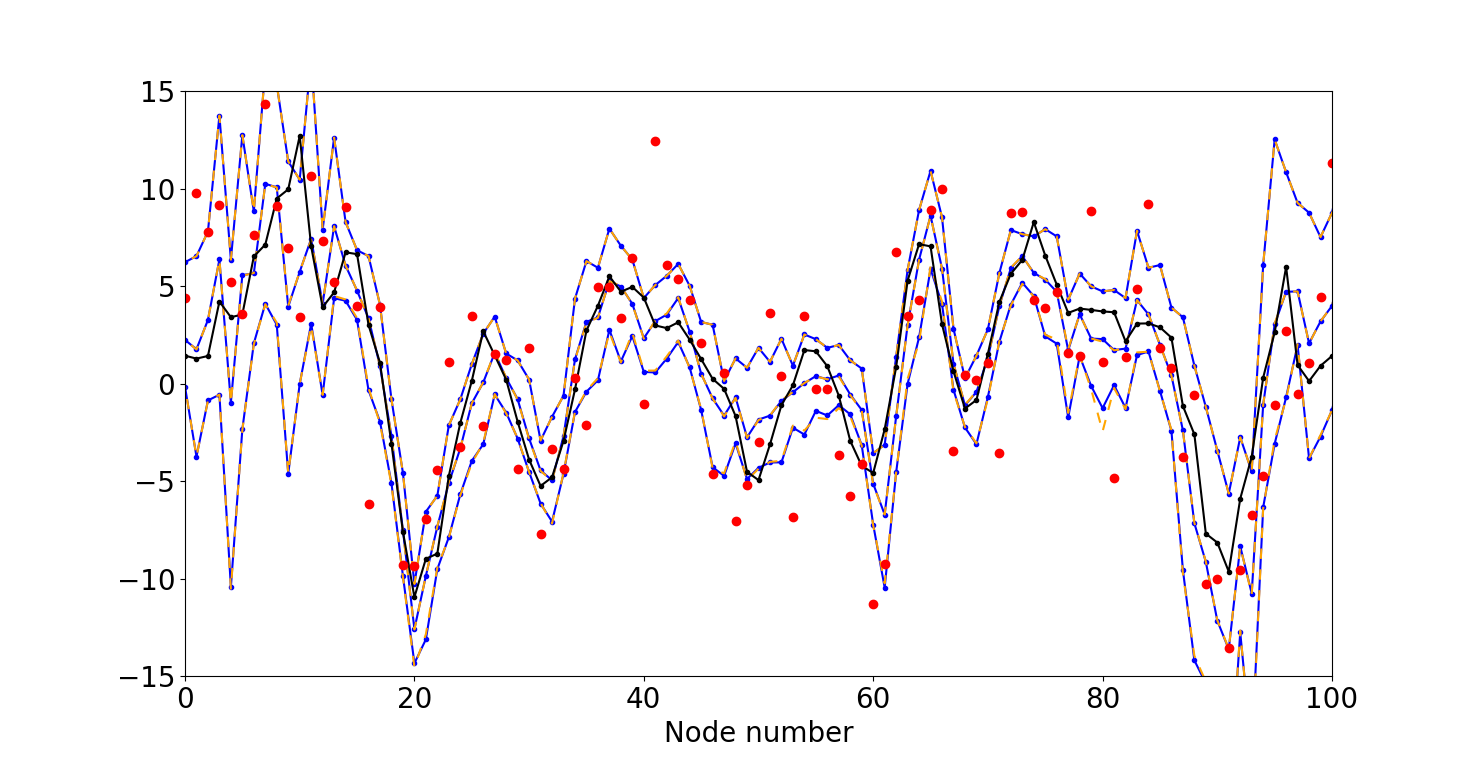
Figure 7: Linear example: Assessment of the approximation error by using the block update at step $t=4$. The figure shows values for nodes $(50,\ell),\ell=1,\ldots,100$. The values of the reference are shown in black and the observations at $t=4$ are shown in red. The ensemble averages and bounds for the empirical $90\%$ credibility intervals when using the optimal model-based EnKF are shown in blue. The corresponding ensemble averages and bounds for the empirical $90\%$ credibility intervals when using the block update are shown in dashed orange

shows results for the nodes $(50,\ell),\ell=1,\ldots,100$ at time step $t=4$. The ensemble averages and bounds of the empirical $90\%$ credibility intervals for the optimal model-based EnKF procedure are shown in blue, and the corresponding values when using the block update procedure for time $t=4$ are shown in dashed orange. For comparison the reference is shown in black. One can observe that for most nodes the mean value and interval bounds when using the block update are visually indistinguishable from the corresponding values when using the block update. The largest difference can be observed for the lower bound of the credibility interval for $\ell=80$. Remembering that we are using blocks of $20\times 20$ nodes in the block update it should not come as a surprise that the largest errors are for values of $\ell$ that are multiples of $20$.

To study the approximation errors in more detail and in particular how the block structure used in the block update influence the approximation, we in Figure 8

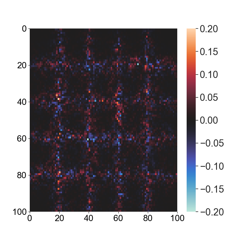
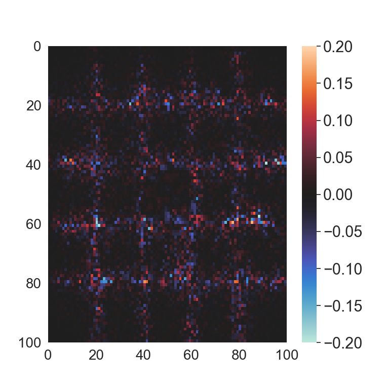
$t=1$		$t=2$
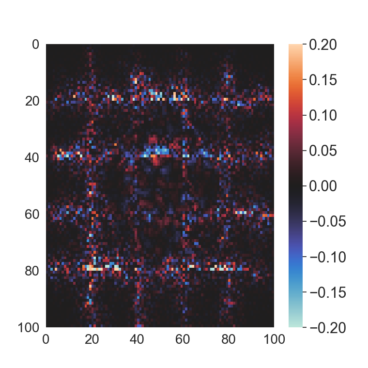
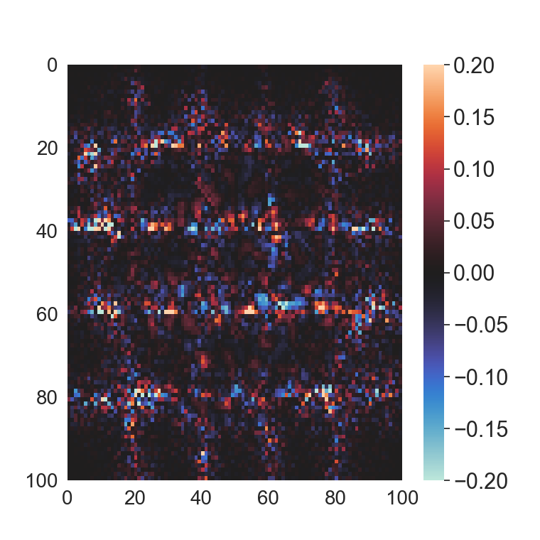
$t=3$		$t=4$
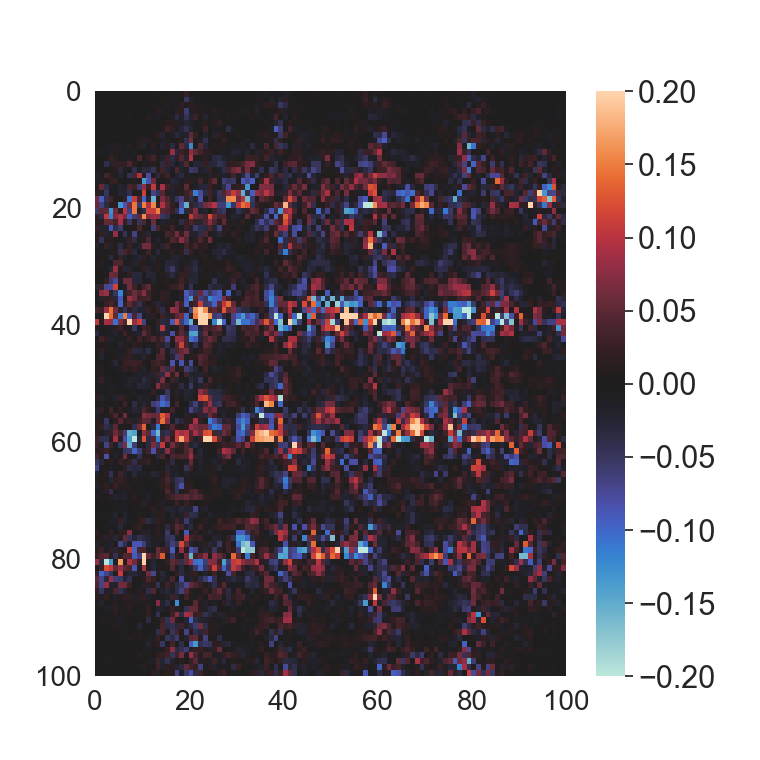
$t=5$

Figure 8: Linear example: Difference between the averages of the ensembles when using the optimal model-based EnKF and when using the block update. Results are shown for each $t=1,\dots,5$

show, for each $t=1,\ldots,5$, the difference between the averages of the ensembles when using the optimal model-based EnKF and when using the block update procedure. As one should expect we see that the largest differences occur along the borders of the $20\times 20$ blocks used in the block update. We can, however, also observe that the magnitude of the errors are all small compared with the spatial variability of the underlying $x_{t}$ process, which explains why the approximation errors are almost invisible in Figure 7.

We then turn our focus to the accumulated effect of the approximation error over several iterations. To do this we again adopt the reference time series and the data described in Section 6.1.1, and the assumed model and algorithmic parameters defined in Section 6.1.2. Based on this we run each of the optimal model-based EnKF and the block update procedures several times, each time with a different initial ensemble and using different random numbers in the updates. For two runs with each of the two filters, Figure 9

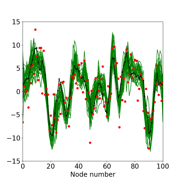
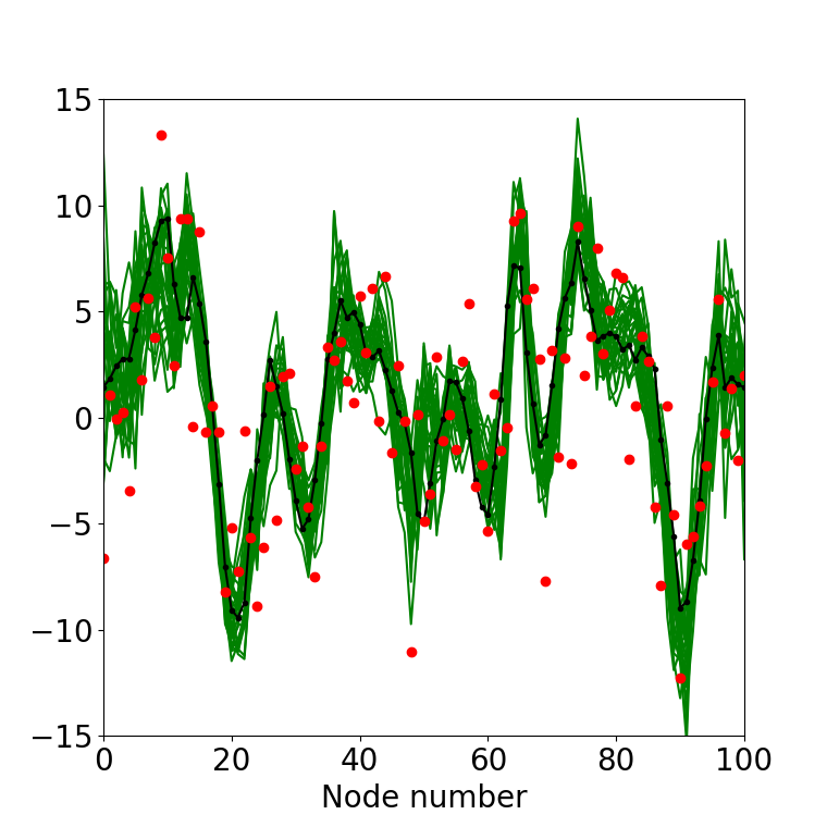
(a)		(b)
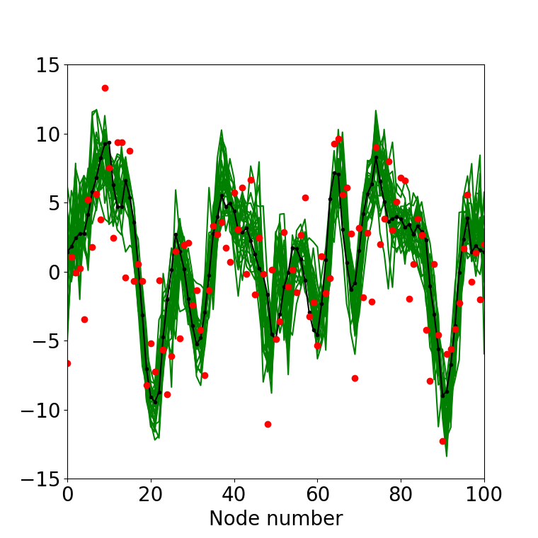
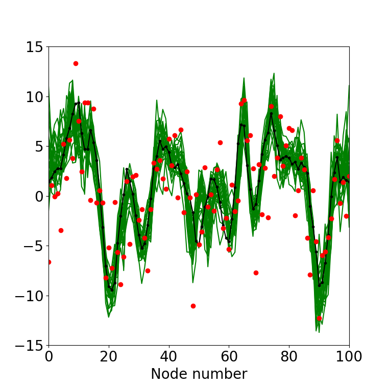
(c)		(d)

Figure 9: Linear example: The reference solution (black) and the observations (red) along one cross section of the grid at time $T=5$. The green lines are the ensemble elements along the same cross section. Figures (a) and (c) show two simulations from the optimal update procedure, while (b) and (d) display two simulations from the block update

shows in green the values of all the ${\mathcal{M}}=25$ ensemble elements in nodes $(50,\ell),\ell=1,\ldots,100$ at time $T=5$. The reference state at $T=5$ is shown in black and the observations at time $T=5$ are again shown as red dots. Figures 9(a) and (c) show results for the optimal model-based EnKF, whereas Figures 9(b) and (d) show results for the proposed block update procedure. Since all four runs are based on the same observations they obviously have many similarities. However, all the ensembles are different. Ensembles updated with the same updating procedure differ because of Monte Carlo variability, i.e. because they used different initial ensembles and different random numbers in the updates. When comparing an ensemble updated with the optimal model-based EnKF procedure with an ensemble updated with the block update, they differ both because of Monte Carlo variability and because of the accumulated effect of the approximation errors up to time $T$. In Figure 9, however, the differences between the ensembles in (a) and (b) and between the ensembles in (c) and (d) seem similar to the differences between the ensembles in (a) and (c) and between the ensembles in (b) and (d). So this indicates that the accumulated effect of the approximation error is small compared to the Monte Carlo variability.

To compare the magnitude of the accumulated approximation error with the Monte Carlo variability in more detail we adopt the two-sample Kolmogorov-Smirnov statistic to measure the difference between the values of two ensembles in one node. More precisely, letting $\widehat{F}_{1}(x\mathchar 24635\relax\;k,\ell)$ and $\widehat{F}_{2}(x\mathchar 24635\relax\;k,\ell)$ denote the empirical distribution functions for the values in node $(k,\ell)$ in two ensembles we use

$$D(k,\ell)=\max_{x}|\widehat{F}_{1}(x\mathchar 24635\relax\;k,\ell)-\widehat{F}_{2}(x\mathchar 24635\relax\;k,\ell)|$$ (53)

to measure the difference between the two ensembles at node $(k,\ell)$. One should note that since we are using ${\mathcal{M}}=25$ elements in each ensemble the $D(k,\ell)$ is a discrete variable with possible values $0.04d\mathchar 24635\relax\;d=0,1,\ldots,25$. Using three runs based on the optimal model-based EnKF we compute $D(k,\ell)$ for each possible pair of ensembles, for each $t=1,\ldots,5$ and for each node in the $100\times 100$ lattice. In Figure 10

$t=1$		$t=2$
$t=3$		$t=4$
$t=5$

Figure 10: Linear example: Histograms of the two-sample Kolmogorov-Smirnov statistics. The statistics computed from two ensembles updated with the optimal ensemble are displayed in blue, while the statistics computed by two ensembles from different updating procedures are visualised in red

histogram of the resulting $30\ 000$ values for each $t=1,\ldots,5$ are shown in blue. Correspondingly we estimate the distribution of $D(k,\ell)$ when one of the ensembles is based on the optimal model-based EnKF and the other is using the block update, and this is shown in red in Figure 10. Comparing the blue and the red histograms for each $t=1,\ldots,5$ in Figure 10 one may arguably see a tendency of the mass in the red histograms to be slightly moved to the right relative to the corresponding blue histograms. This is as one would expect, but we also observe that the effect of the approximation error is negligible compared to the Monte Carlo variability.

6.1.5 Comparison of the results with the Kalman filter output

Since the forward model in this numerical example is linear and deterministic and the observation model is Gauss-linear, we are able to compare the block update to the Kalman filter solution. Figure 11

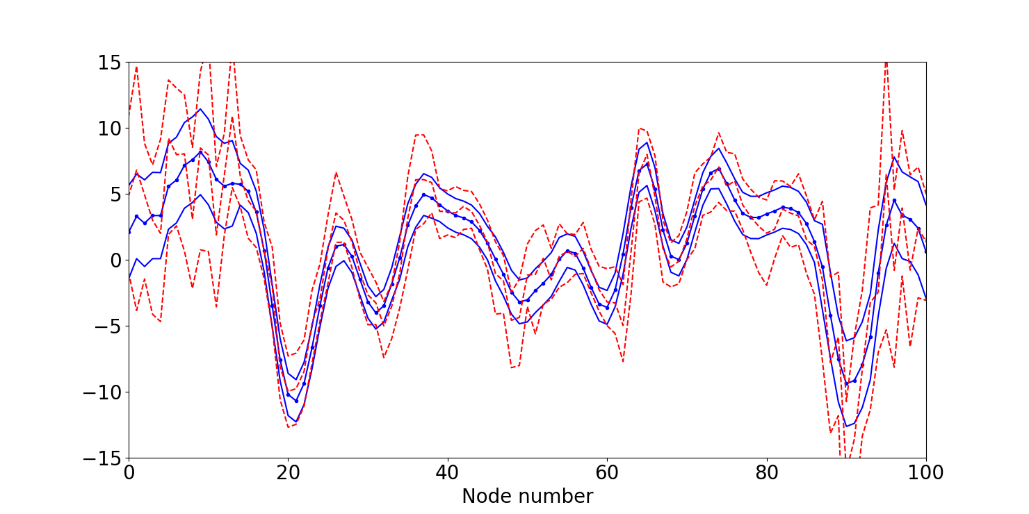
Figure 11: Linear example: The blue lines display the mean of the Kalman filter solution along with the $90\%$ credibility intervals for one cross section at time $t=4$. The red lines visualise the empirical mean and empirical $90\%$ credibility interval for the block update for the same cross section at the same time step.

displays the mean of the Kalman filter solution along with the $90\%$ credibility interval for the nodes $(50,\ell),l=1,\ldots,100$ in blue at $t=4$. The red lines visualise the empirical mean and empirical $90\%$ credibility interval as given by one simulation of the block update. When comparing the two set of curves one should remember that the EnKF output is stochastic, so for another EnKF run a different set of curves would be produced. In general, however, we notice that the mean given by the block update follows the mean of the Kalman filter quite well.

When comparing the credibility intervals we can observe that the intervals provided by the block update appears to be somewhat longer than the credibility intervals provided by the Kalman filter. This is as one should expect. At each step of the block update filter, as for any other ensemble based filter, we represent the credibility and filtering distribution by a rather small set of realisations. So compared to the Kalman filter, where the exact credibility and filtering distributions are represented by mean vectors and covariance matrices, we necessarily loose some information about the the underlying true state vector at each iteration of the block update filter, when representing the distributions by a set of realisations only.

The results for times $t=1,2,3$ and $5$ are similar to the results for time $t=4$, except that the widths of the credibility intervals decrease with time. The shrinkage of the widths of the credibility intervals is clearly visible for both the Kalman filter and the block update filter, but is stronger for the Kalman filter than for the block update filter. Such a shrinkage is as one should expect when the forward function is deterministic. That the shrinkage is strongest for the Kalman filter is reasonable since in each iteration of block update filter we loose some information about the underlying true state when just representing the distributions by ensembles.

6.2 Non-linear example

In the following we consider a non-linear example. We first describe how the reference solution and observations are generated, before we proceed to compare the results provided by the block update filter with the results of the optimal model-based EnKF.

6.2.1 Reference time series and observations

The reference state for the initial time step, $x_{1}$, is generated in the exact same manner as for the linear case. The forward model used is inspired by the non-linear forward function in HEnKF. The forward function is acting on each element of the state vector separately. The reference state at time $t>1$ for node $(k,\ell)$ is defined by

$$x_{t}^{(k-1)\cdot s+\ell}=x_{t-1}^{(k-1)\cdot s+\ell}+0.5\cdot\arctan\left(\frac{x_{t-1}^{(k-1)\cdot s+\ell}}{2}\right).$$ (54)

The term $0.5\cdot\arctan(x/2)$ is chosen to make the forward function clearly non-linear over the interval in which the elements of the state vector vary. The term is displayed in Figure 12.

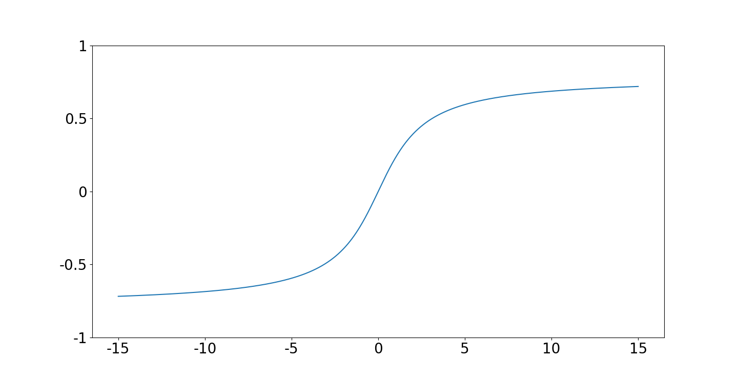
Figure 12: Non-linear example: The term $0.5\cdot\arctan(x/2)$ in the forward function of the non-linear example

The observations are generated in the exact same manner as in the linear example. The assumed model and all the algorithmic parameters are also chosen identical to what we used in the linear example.

6.2.2 Approximation error in block update

As for the linear example, we first consider the approximation error obtained in one update, and thereafter study how the approximation error accumulates over multiple iterations.

To study the effect of the approximation error in one iteration we follow the same procedure as used in Section 6.1.4. In Figure 13

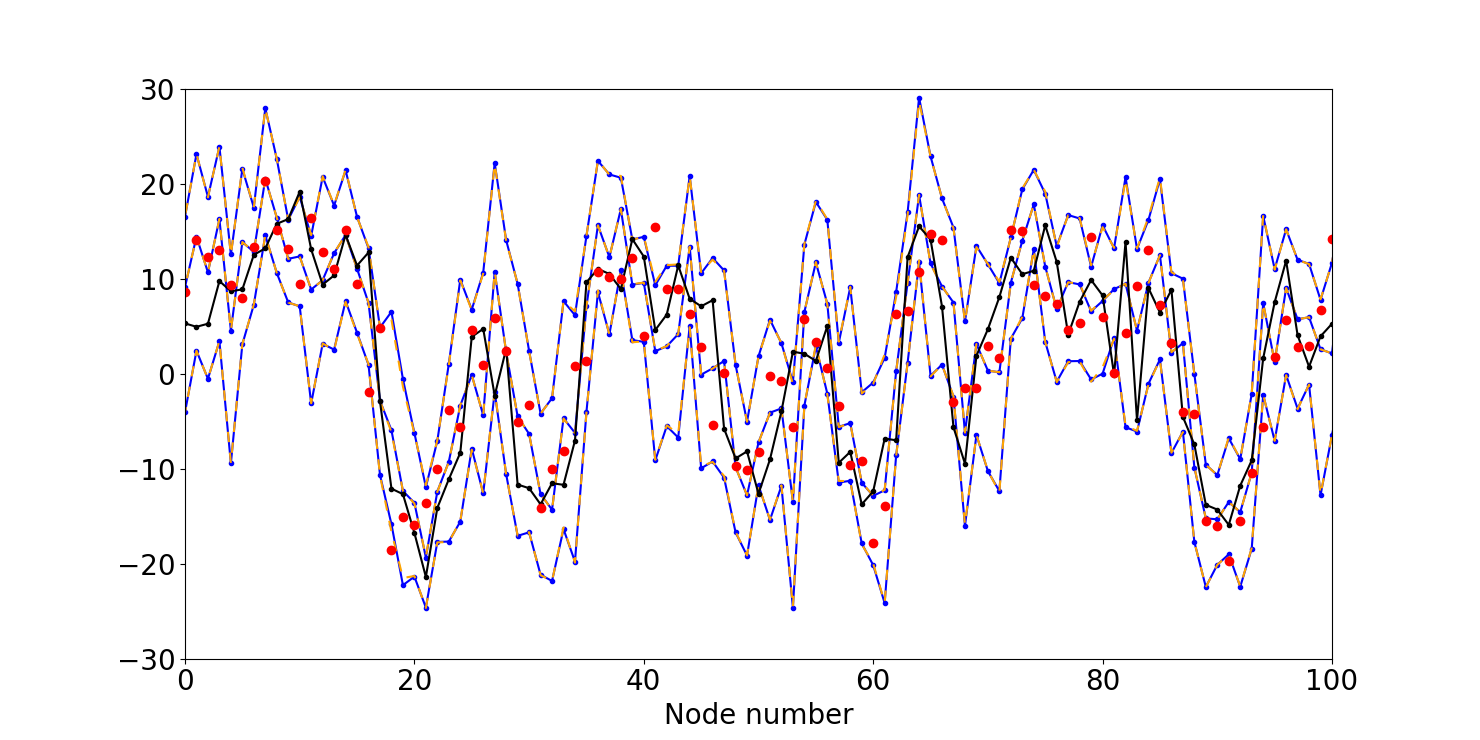
Figure 13: Non-linear example: Assessment of the approximation error by using the block update at step $t=4$. The figure shows values for nodes $(50,\ell),\ell=1,\ldots,100$. The values of the reference are shown in black and the observations at $t=4$ are shown in red. The ensemble averages and bounds for the empirical $90\%$ credibility intervals when using the optimal model-based EnKF are shown in blue. The corresponding ensemble averages and bounds for the empirical $90\%$ credibility intervals when using the block update are shown in dashed orange

we compare the credibility intervals provided by the optimal update and block update at time $t=4$, similar to Figure 7 for the linear case. The credibility interval for the nodes $(50,\ell)$, $\ell=1,\ldots,100$ provided by the optimal update is displayed in blue, while the credibility interval provided by the block update is visualised in orange. We notice that the credibility intervals provided by the two update procedures are practically speaking visually indistinguishable, similar to what we observe for the linear case. We have also studied the spatial variability of the approximation errors by inspecting plots of the difference of the means of the ensembles provided by the two update procedures, similar to Figure 8. The results for the non-linear example are similar to what we observed in the linear case. The largest approximation errors are again concentrated around the block borders, and the relative approximation errors are similar to what we had with the linear forward function.

To study how the approximation errors accumulated over several iterations, we followed the same procedure as in the linear example. When comparing ensembles resulting from the two filters, corresponding to what is done in Figure 9, the accumulated effect of the approximation error again seem to be small compared to the Monte Carlo variability. Figure 14

$t=1$		$t=2$
$t=3$		$t=4$
$t=5$

Figure 14: Non-linear example: Histograms of the two-sample Kolmogorov-Smirnov statistics. The statistics computed from two ensembles updated with the optimal ensemble are displayed in blue, while the statistics computed by two ensembles from different updating procedures are visualised in red

displays the histograms of the Kolmogorov-Smirnov statistics for $t=1,\ldots,5$, analogous to Figure 10 for the linear case. We arguably can observe that the tendency of the mass in the red histograms to be moved to the right compared to the corresponding blue histograms, is slightly stronger in this non-linear example than in the linear case.

7 Closing remarks

In this paper we propose two changes in the model-based EnKF procedure introduced in LoeTjelmeland2021. Our motivation is to get a procedure that is computationally faster than the original one, so that it is feasible to use it also in situations with high dimensional state vectors. The first change we introduce is to formulate the assumed model in terms of precision matrices instead of covariance matrices, and to adopt a prior for the precision matrix that ensures the sampled precision matrices to be sparse. The second change we propose is to adopt the block update, which allows us to do singular value decompositions of many smaller matrices instead of for one large one.

In a simulation example we have studied both the computational speedup and the associated approximation error resulting when adopting the proposed procedure. The computational speedup is substantial for high dimensional state vectors and this allows the proposed filter to be run on much larger problems than can be done with the original formulation. At the same time the approximation error resulting from using the introduced block updating is negligible compared to the Monte Carlo variability inherent in both the original and the proposed procedures.

In order to further investigate the strengths and weaknesses of the proposed approach, it should be applied on more examples. It is of interest to gain more experience with the proposed procedure both in other simulation examples and in real data situations. In particular it is of interest to experiment more with different sizes for the $C_{b}$, $D_{b}$ and $E_{b}$ blocks to try to find the best sizes for these when taking both the computational time and the approximation quality into account. As for all EnKFs the proposed procedure is ideal for parallel computation and with an implementation more tailored for parallellisation it should be possible get a code that is running much faster than our more basic implementation.