cuFasterTucker: A Stochastic Optimization Strategy for Parallel Sparse FastTucker Decomposition on GPU Platform

Abstract

Currently, the size of scientific data is growing at an unprecedented rate. Data in the form of tensors exhibit high-order, high-dimensional, and highly sparse features. Although tensor-based analysis methods are very effective, the large increase in data size makes the original tensor impossible to process. Tensor decomposition decomposes a tensor into multiple low-rank matrices or tensors that can be exploited by tensor-based analysis methods. Tucker decomposition is such an algorithm, which decomposes a $n$-order tensor into $n$ low-rank factor matrices and a low-rank core tensor. However, most Tucker decomposition methods are accompanied by huge intermediate variables and huge computational load, making them unable to process high-order and high-dimensional tensors.

In this paper, we propose FasterTucker decomposition based on FastTucker decomposition, which is a variant of Tucker decomposition. And an efficient parallel FasterTucker decomposition algorithm cuFasterTucker on GPU platform is proposed. It has very low storage and computational requirements, and effectively solves the problem of high-order and high-dimensional sparse tensor decomposition. Compared with the state-of-the-art algorithm, it achieves a speedup of around $15X$ and $7X$ in updating the factor matrices and updating the core matrices, respectively.

I Introduction

Tensors are extensions of vectors and matrices, and are a general term for three-order or higher-order data[1]. Data derived from the real world is usually high-order and can naturally be represented by tensors[2]. For example, an image is a $3$-order tensor, and a video is a $4$-order tensor. Tensors can clearly represent the complex interaction of multiple features of an entity, which cannot be represented using linear or planar data forms. As tensor data becomes higher in order and larger in scale, it is no longer practical to analyze full tensors directly. The tensor decomposition, which uses multiple low-rank feature matrices or tensors to represent the original tensor and preserves the multi-order structural information of the original tensor, emerges as the times require. At present, tensor methods based on tensor decomposition have been widely used in recommender system[3], social network[4], psychological testing[5], biology[6], stoichiometry[7], cryptography[8], signal processing[9], deep learning [10, 11], numerical analysis [12] and other fields.

Tucker decomposition[13] is one of the mainstream tensor decomposition algorithms, and it is a generalization of Singular Value Decomposition (SVD) for high-order data. It decomposes an $n$-order tensor into $n$ low-rank factor matrices and a low-rank core tensor. These factor matrices extract important features of different orders respectively, and the core tensor reflects the interaction between different orders. Tucker decomposition is usually implemented by the Higher Order Singular Value Decomposition (HOSVD) algorithm[14] or the Higher Order Orthogonal Iteration (HOOI) algorithm[15]. HOSVD algorithm flattens each order of the original tensor and does SVD operations, with huge memory overhead and computational complexity for intermediate matrices[16]. Some variants of HOSVD algorithm were proposed, such as Truncated HOSVD (T-HOSVD) [17, 18], Sequentially Truncated HOSVD (ST-HOSVD)[19], Hierarchical HOSVD[20], but did not solve the problem fundamentally. The operation of Tensor Multiplying Matrix Chain (TTMc) in HOOI algorithm also has huge intermediate variables and computational complexity, which is its computational bottleneck. Some variants of the Alternating Least Squares(ALS)-based HOOI algorithm have attempted to address these issues, such as, P-Tucker[21], Vest[22], ParTi[23] and GTA[24], with little success.

The scale of data derived from multiple relational interactions is growing at an unprecedented rate, such as recommender systems[25], Quality of Service (QoS)[26], social networks [27], etc., forming High-Order, High-Dimension, and Sparse Tensor (HOHDST). To compress and process these HOHDST, which cannot even be stored and computed in a single machine, we need efficient and scalable parallel algorithms. Some parallel sparse Tucker decomposition algorithms on different parallel platforms have made some progress on the above problem. But they still have high intermediate variable storage and high computational complexity and scalability issues. The FastTucker proposed in [28] replaces the $n$-order core tensor with $n$ low-rank core matrices, reduces the space complexity and computational complexity of Tucker decomposition from exponential to polynomial level, and keeps the solution space of Tucker decomposition unchanged. However, its parallel algorithm cuFastTucker on the GPU platform has a large number of redundant calculations, and its utilization efficiency of the GPU is not ideal.

In this paper, we propose cuFasterTucker, a stochastic optimization strategy for parallel sparse FastTucker decomposition on GPU Platform. It updates one factor matrix or core matrix at a time and fixes other factor matrices and core matrices, which ensures that it is a convex optimization problem every time. cuFasterTucker uses the Balanced Compressed Sparse Fiber (B-CSF) tensor storage format[29], which increases the memory access efficiency while ensuring a relatively balanced load, and reduces the calculation of shared intermediate variables. More importantly, cufast stores reusable intermediate variables, which only occupy a small amount of memory, but greatly reduce its computational complexity.

Our main contributions are the following:

1. Algorithm. We propose cuFasterTucker, a stochastic optimization strategy for parallel sparse FastTucker decomposition on GPU Platform. It reduces the computation of reusable intermediate variables and shared intermediate variables, and makes full use of GPU storage resources. It works fine on HOHDST data.

2. Theory. We analyze the computational complexity of the main process of cuFastTucker and cuFasterTucker, and prove that cuFasterTucker reduces the computational complexity from $(N-1)|\Omega|\sum J_{n}R$ $to$ $\sum I_{n}J_{n}R$.

3. Performance. Before cuFasterTucker, cuFastTucker was the known optimal parallel sparse Tucker decomposition algorithm capable of handling hosterge data. Experiments show that compared with cuFastTucker, cuFasterTucker achieves about $15.0X$ and $7.0X$ speedup in update factor matrices and update core matrices, respectively. In addition, cuFasterTucker is more suitable for processing higher-order tensors than cuFastTucker, because cuFasterTucker takes much less time than cuFastTucker.

The code of cuFasterTucker used in this paper and a toy dataset are available at https://github.com/ZixuanLi-China/cuFasterTucker for reproducibility. The rest of this paper is organized as follows. Section II introduces the notations, definitions, tensor operations, and FastTucker decomposition. Section III describes our proposed method FasterTucker decomposition. Section IV describes our proposed fine-grained parallel sparse FasterTucker algorithm cuFasterTucker on GPU platform. Section V presents experimental results of cuFasterTucker andits contrasting algorithms. And Section VI summarizes our work.

II Preliminaries

We describe the notations in this paper in Section II-A, definitions in Section II-B, and FastTucker decomposition in II-C and Stochastic Gradient Descent (SGD) based sparse FastTucker decomposition in II-D. Notations are summarized in Table I.

II-A Notations

We denote tensors by bold Euler script letters (such as $\bm{\mathcal{X}}$), matrices by bold uppercase (such as A), vectors by bold lowercase (such as a), scalars by regular lowercase or uppercase (such as $N$ and $k$). The elements in the tensor are denoted by the symbolic name of the tensor and the index, for example, $x_{i_{1},i_{2},\cdots,i_{n}}$ denotes the $(i_{1},i_{2},\cdots,i_{n})$th element of the tensor $\bm{\mathcal{X}}$. And, $\textbf{a}_{i}$ denotes the $i$th row of matrix A, $\textbf{a}_{:,j}$ denotes the $j$th column of matrix A.

TABLE I: Table of symbols.

Symbol	Definition
$\bm{\mathcal{X}}$	Input $N$-order tensor $\in$ $\mathbb{R}^{I_{1}\times I_{2}\times\cdots\times I_{N}}$;
$x_{i_{1},i_{2},\cdots,i_{n}}$	$i_{1},i_{2},\cdots,i_{n}$th element of tensor $\mathcal{X}$
$\{N\}$	The ordered set $\{1,2,\cdots,N-1,N\}$
$\{R\}$	The core index set $\{1,2,\cdots,R-1,R\}$
$\{I_{n}\}$	The index set $\{1,2,\cdots,I_{n}-1,I_{n}\}$
$\Omega$	Index $(i_{1},\cdots,i_{n},\cdots,i_{N})$ of a tensor $\mathcal{X}$
$\textbf{A}^{(n)}$	$n$th factor matrix $\in$ $\mathbb{R}^{I_{n}\times J_{n}}$
$\textbf{B}^{(n)}$	$n$th core matrix $\in$ $\mathbb{R}^{J_{n}\times R}$
$a_{i_{n},:}^{(n)}$	$i_{n}$th row vector $\in$ $\mathbb{R}^{J_{n}}$ of $\textbf{A}^{(n)}$
$b_{:,r}^{(n)}$	$r$th column vector $\in$ $\mathbb{R}^{J_{n}}$ of $\textbf{B}^{(n)}$
$\circ$	Outer product
$\times$	Matrix product
$\times_{(n)}$	$n$-Mode Tensor-Matrix product
$\otimes$	Kronecker product
$\%$	Remainder

II-B Basic Definitions

Definition 1 ($n$-Mode Tensor Matricization)

Given a $N$-order tensor $\bm{\mathcal{X}}$ $\in$ $\mathbb{R}^{I_{1}\times\cdots\times I_{N}}$, $n$-Mode Tensor Matricization refers to that $\bm{\mathcal{X}}$ is unfolded in the $n$th order to form a low order matrix $\textbf{X}^{(n)}\in\mathbb{R}^{I_{n}\times I_{1}\cdots I_{n-1}\cdot I_{n+1}\cdot\cdots\cdot I_{N}}$, where $\textbf{X}^{(n)}$ stores all element of the $\bm{\mathcal{X}}\in\mathbb{R}$ and the matrix element $x^{(n)}_{i_{n},j}$ of $\textbf{X}^{(n)}$ at the position $j=1+\sum_{k=1,n\neq k}^{N}\left[(i_{k}-1)\mathop{\prod}_{m=1,m\neq n}^{k-1}I_{m}\right]$ contains the tensor element $x_{i_{1},i_{2},\cdots,i_{n},\cdots,i_{N}}$ of the tensor $\bm{\mathcal{X}}$.

Definition 2 ($n$-Mode Tensor Vectorization)

Given a $N$-order tensor $\bm{\mathcal{X}}$ $\in$ $\mathbb{R}^{I_{1}\times\cdots\times I_{N}}$, $n$-Mode Tensor Vectorization refers to that $\bm{\mathcal{X}}$ is unfolded in the $n$th order to form a vector $\textbf{x}^{(n)}$, where $\textbf{x}^{(n)}$ stores all element of the $\bm{\mathcal{X}}\in\mathbb{R}$ and the vector element $x^{(n)}_{k}$ of $\textbf{x}^{(n)}$ at the position $k=(j-1)I_{n}+i$ contains the tensor element $\textbf{X}^{(n)}_{i,j}$ of $n$th matricization $\textbf{X}^{(n)}$ of a tensor $\mathcal{X}$.

Definition 3 ($n$-Mode Tensor-Matrix product)

Given a $N$-order tensor $\bm{\mathcal{X}}$ $\in$ $\mathbb{R}^{I_{1}\times\cdots\times I_{N}}$ and a matrix A $\in$ $\mathbb{R}^{J_{n}\times I_{n}}$, $n$-Mode Tensor-Matrix product projects $\bm{\mathcal{X}}$ and A to a new tensor $(\bm{\mathcal{X}}\times_{(n)}\textbf{A})$ $\in$ $\mathbb{R}^{I_{1}\times\cdots\times I_{n-1}\times J_{n}\times I_{n+1}\times\cdots I_{N}}$ according to the coordinates, where $(\bm{\mathcal{X}}\times_{(n)}\textbf{A})_{i_{1}\times\cdots\times i_{n-1}\times j_{n}\times i_{n+1}\times\cdots\times i_{N}}$ $=$ $\sum\limits_{i_{n}=1}^{I_{n}}$ $x_{i_{1}\times\cdots\times i_{n}\times\cdots\times i_{N}}$ $\cdot a_{j_{n},i_{n}}$.

Definition 4 (Rank-one Tensor)

Given a $N$-order tensor $\bm{\mathcal{X}}$ $\in$ $\mathbb{R}^{I_{1}\times\cdots\times I_{N}}$, $\bm{\mathcal{X}}$ is Rank-one Tensor if it can be written as the outer product of N vectors, i.e., $\bm{\mathcal{X}}$ $=$ $b^{(1)}\circ b^{(2)}\circ\cdots\circ b^{(n)}$.

Definition 5 (The Rank of a Tensor)

Given a $N$-order tensor $\bm{\mathcal{X}}$ $\in$ $\mathbb{R}^{I_{1}\times\cdots\times I_{N}}$, the rank of $\bm{\mathcal{X}}$, denoted $rank_{n}(\bm{\mathcal{X}})$, is defined as the smallest number of Rank-one Tensors that generate $\bm{\mathcal{X}}$ as their sum.

Definition 6 ($R$ Kruskal Product)

Given $N$ matrices $\textbf{B}^{(n)}$ $\in$ $\mathbb{R}^{I_{n}\times R}$, $n\in\{N\}$, a $N$-order tensor $\widehat{\bm{\mathcal{X}}}$ $\in$ $\mathbb{R}^{I_{1}\times\cdots\times I_{N}}$ can be obtained by $R$ Kruskal Product: $\widehat{\bm{\mathcal{X}}}=\sum_{r=1}^{R}b^{(1)}_{:,r}\circ\cdots\circ b^{(n)}_{:,r}\circ\cdots\circ b^{(N)}_{:,r}$.

Definition 7 (Khatri-Rao product)

Given a matrice A $\in$ $\mathbb{R}^{I\times K}$ and a matrice B $\in$ $\mathbb{R}^{J\times K}$, Khatri-Rao product projects A and B to a new matrice $(\textbf{A}\odot\textbf{B})$ $\in$ $\mathbb{R}^{IJ\times K}$ according to the coordinates, where $(\textbf{A}\odot\textbf{B})_{m,n}$ $=$ $\textbf{a}_{i/I,n}$ $\cdot$ $\textbf{b}_{m\%J,n}$.

Definition 8 (Kronecker product)

Given a matrice A $\in$ $\mathbb{R}^{I\times J}$ and a matrice B $\in$ $\mathbb{R}^{K\times L}$, Kronecker product projects A and B to a new matrice $(\textbf{A}\otimes\textbf{B})$ $\in$ $\mathbb{R}^{IK\times JL}$ according to the coordinates, where $(\textbf{A}\otimes\textbf{B})_{m,n}$ $=$ $\textbf{a}_{m/I,n/J}$ $\cdot$ $\textbf{b}_{m\%K,n\%L}$.

Definition 9 (Tensor Approximation)

Given a $N$-order sparse tensor $\bm{\mathcal{X}}$ $\in$ $\mathbb{R}^{I_{1}\times\cdots\times I_{N}}$, the Tensor Approximation is to find a low-rank tensor $\widehat{\bm{\mathcal{X}}}$ $\in$ $\mathbb{R}^{I_{1}\times\cdots\times I_{N}}$ such that $\mathcal{D}(\bm{\mathcal{E}})$ small enough, where noisy tensor $\bm{\mathcal{E}}=$$\bm{\mathcal{X}}-\widehat{\bm{\mathcal{X}}}$$\in$ $\mathbb{R}^{I_{1}\times\cdots\times I_{N}}$ and $\mathcal{D}$ is a norm function.

II-C FastTucker Decomposition

Tensor decomposition is a solution to tensor approximation. Commonly used tensor decomposition methods include Canonical Polyadic (CP) decomposition, Tucker decomposition and FastTucker decomposition. Our proposed method FasterTucker is based on FastTucker decomposition. Given a $N$-order tensor $\bm{\mathcal{X}}$ $\in$ $\mathbb{R}^{I_{1}\times\cdots\times I_{N}}$, the goal of FastTucker decomposition is to find $N$ factor matrices $\textbf{A}^{(n)}$ $\in$ $\mathbb{R}^{I_{n}\times J_{n}}$,$J_{n}\ll rank_{n}(\mathcal{X})$, $n\in\{N\}$ and $N$ core matrices $\textbf{B}^{(n)}$ $\in$ $\mathbb{R}^{J_{n}\times R}$, $n\in\{N\}$, such that:

$$\bm{\mathcal{X}}\approx\widehat{\bm{\mathcal{X}}}= \bigg{(}\sum_{r=1}^{R}b^{(1)}_{:,r}\circ\cdots\circ b^{(n)}_{:,r}\circ\cdots\circ b^{(N)}_{:,r}\bigg{)}\times_{(1)}\textbf{A}^{(1)}\times_{(2)}$$ (1)

$$\cdots\times_{(n)}\textbf{A}^{(n)}\times_{(n+1)}\cdots\times_{(N)}\textbf{A}^{(N)}$$

In fact, FastTucker decomposition further decomposes the $N$-order core tensor in the tucker decomposition into N core matrices.

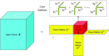
Figure 1: An example of FastTucker

We let $\mathcal{D}$ be the Frobenius Norm, in order to make $\mathcal{D}(\bm{\mathcal{X}}-\widehat{\bm{\mathcal{X}})}$ as small as possible, it is transformed into the following optimization problem:

$$\mathop{\arg\min}_{\textbf{A}^{(n)},n\in\{N\},\textbf{B}^{(n)},n\in\{N\}}f\bigg{(}\bm{\mathcal{X}},\big{\{}\textbf{A}^{(n)}\big{\}},\big{\{}\textbf{B}^{(n)}\big{\}},n\in\{N\}\bigg{)}$$ (2)

$$=\bigg{\|}\bm{\mathcal{X}}-\widehat{\bm{\mathcal{X}}}\bigg{\|}_{2}^{2}+\sum_{n=1}^{N}\lambda_{\textbf{A}^{(n)}}\|\textbf{A}^{(n)}\|_{2}^{2}+\sum_{n=1}^{N}\lambda_{\textbf{B}^{(n)}}\|\textbf{B}^{(n)}\|_{2}^{2}$$

where $\lambda_{\textbf{A}^{(n)}},n\in\{N\}$ and $\lambda_{\textbf{B}^{(n)}},n\in\{N\}$ are the regularization parameters for low-rank factor matrices $\textbf{A}^{(n)},n\in\{N\}$ and core matrices $\textbf{B}^{(n)},n\in\{N\}$, respectively.

The optimization objective (2) involves variables multiplication, which is non-convex. The non-convex problem can be tackled by convex solution via updating a variable and fixing the others. And the matricized version of equation (1) is

$$\widehat{\textbf{X}}^{(n)}= \textbf{A}^{(n)}(\textbf{B}^{(n)}(\textbf{B}^{(N)}\odot\cdots\odot\textbf{B}^{(n+1)}\odot\textbf{B}^{(n-1)}\odot\cdots$$ (3)

$$\odot\textbf{B}^{(1)})^{T})(\textbf{A}^{(N)}\otimes\cdots\otimes\textbf{A}^{(n+1)}\otimes\textbf{A}^{(n-1)}\otimes\cdots$$

$$\otimes\textbf{A}^{(1)})^{T}$$

where $\widehat{\textbf{X}}^{(n)}$ is $n$th matricization of tensor $\widehat{\bm{\mathcal{\bm{X}}}}$. The optimization problem (2) can be split into updating low-rank factor matrices $\textbf{A}^{(n)},n\in\{N\}$ and updating core matrices $\textbf{B}^{(n)},n\in\{N\}$ as following:

$$\mathop{\arg\min}_{\textbf{A}^{(n)},n\in\{N\}} f\bigg{(}\textbf{A}^{(n)}\bigg{|}\textbf{X}^{(n)},\big{\{}\textbf{A}^{(n)}\big{\}},\big{\{}\textbf{B}^{(n)}\big{\}},n\in\{N\}\bigg{)}$$ (4)

$$=\bigg{\|}\textbf{X}^{(n)}-\widehat{\textbf{X}}^{(n)}\bigg{\|}_{2}^{2}+\lambda_{\textbf{A}^{(n)}}\|\textbf{A}^{(n)}\|_{2}^{2}$$

and

$$\mathop{\arg\min}_{\textbf{B}^{(n)},n\in\{N\}} f\bigg{(}\textbf{B}^{(n)}\bigg{|}\textbf{X}^{(n)},\big{\{}\textbf{A}^{(n)}\big{\}},\big{\{}\textbf{B}^{(n)}\big{\}},n\in\{N\}\bigg{)}$$ (5)

$$=\bigg{\|}\textbf{X}^{(n)}-\widehat{\textbf{X}}^{(n)}\bigg{\|}_{2}^{2}+\lambda_{\textbf{B}^{(n)}}\|\textbf{B}^{(n)}\|_{2}^{2}$$

where $\widehat{\textbf{X}}^{(n)}$ $=$ $\textbf{A}^{(n)}\textbf{B}^{(n)}\textbf{Q}^{(n)^{T}}\textbf{S}^{(n)^{T}}$, $\textbf{S}^{(n)}$ $=$ $\textbf{A}^{(N)}\otimes\cdots\otimes\textbf{A}^{(n+1)}\otimes\textbf{A}^{(n-1)}\otimes\cdots\otimes\textbf{A}^{(1)}$ and $\textbf{Q}^{(n)}$ $=$ $\textbf{B}^{(N)}\odot\cdots\odot\textbf{B}^{(n+1)}\odot\textbf{B}^{(n-1)}\odot\cdots\odot\textbf{B}^{(1)}$.

For any $n\in\{N\}$, optimization objectives (4) and (5) are both convex optimization problems, and the smaller the value of the loss function, the smaller the value of the loss function of optimization objective (2). Solving convex optimization problems can make the value of the loss function keep decreasing, and by solving these optimization objectives in a loop, the non-convex optimization objective can finally reach convergence.

II-D Sparse FastTucker Decomposition

Note that the optimization objectives (2), (4) and (5) are calculated by all elements of $\bm{\mathcal{X}}$, and whole missing values of $\bm{\mathcal{X}}$ are regarded as zeros. In fact, most tensors are extremely sparse, and it is unreasonable to treat all missing elements as zeros. We denote the set of observable elements in $\bm{\mathcal{X}}$ as $\Omega$, and the number of elements in $\Omega$ as $|\Omega|$. Sparse FastTucker decomposition finds $\textbf{A}^{(n)},n\in\{N\}$ and $\textbf{B}^{(n)},n\in\{N\}$ only by optimization objective (6) with the elements present in $\bm{\mathcal{X}}$, and predicts values of missing elements after $\textbf{A}^{(n)},n\in\{N\}$ and $\textbf{B}^{(n)},n\in\{N\}$ are found.

$$\mathop{\arg\min}_{\textbf{A}^{(n)},n\in\{N\},\textbf{B}^{(n)},n\in\{N\}}f\bigg{(}\bm{\mathcal{X}},\big{\{}\textbf{A}^{(n)}\big{\}},\big{\{}\textbf{B}^{(n)}\big{\}},n\in\{N\}\bigg{)}$$ (6)

$$= \sum_{x_{i_{1},\dots,i_{N}}\in\Omega}\bigg{\|}x_{i_{1},\dots,i_{N}}-\widehat{x}_{i_{1},\dots,i_{N}}\bigg{\|}_{2}^{2}+\sum_{n=1}^{N}\lambda_{\textbf{A}^{(n)}}\|\textbf{A}^{(n)}\|_{2}^{2}$$

$$+\sum_{n=1}^{N}\lambda_{\textbf{B}^{(n)}}\|\textbf{B}^{(n)}\|_{2}^{2}$$

In fact, the overall optimization problem (6) can be decomposed into multiple single-element optimization problems. Similar to the dense FastTucker, the overall optimization problem (6) can be solved by alternately solving convex factor matrix optimization problem (7)

$$\mathop{\arg\min}_{\textbf{a}^{(n)}_{i_{n}},n\in\{N\}}f\bigg{(}\textbf{a}^{(n)}_{i_{n}}\bigg{|}x_{i_{1},\dots,i_{N}},\big{\{}\textbf{A}^{(n)}\big{\}},\big{\{}\textbf{B}^{(n)}\big{\}},n\in\{N\}\bigg{)}$$ (7)

$$=\bigg{\|}x_{i_{1},\dots,i_{N}}-\widehat{x}_{i_{1},\dots,i_{N}}\bigg{\|}_{2}^{2}+\lambda_{\textbf{a}^{(n)}_{i_{n}}}\|\textbf{a}^{(n)}_{i_{n}}\|_{2}^{2}$$

and convex core matrix optimization problem (8)

$$\mathop{\arg\min}_{\textbf{b}^{(n)}_{:,r},n\in\{N\},r\in\{R\}}f\bigg{(}\textbf{b}^{(n)}_{:,r}\bigg{|}x_{i_{1},\dots,i_{N}},\big{\{}\textbf{A}^{(n)}\big{\}},\big{\{}\textbf{B}^{(n)}\big{\}},n\in\{N\}\bigg{)}$$ (8)

$$=\bigg{\|}x_{i_{1},\dots,i_{N}}-\widehat{x}_{i_{1},\dots,i_{N}}\bigg{\|}_{2}^{2}+\lambda_{\textbf{b}^{(n)}_{:,r}}\|\textbf{b}^{(n)}_{:,r}\|_{2}^{2}$$

In large-scale optimization scenarios, SGD is a common strategy and promises to obtain the optimal accuracy via a certain number of training epoches. An $M$ elements set $\Psi$ is randomly selected from the set $\Omega$, the learning rate is $\gamma$, and the SGD is presented as:

$$w \leftarrow w-\gamma\frac{\partial f_{\Psi}(w)}{\partial w}$$ (9)

$$=w-\gamma\frac{1}{M}\sum_{i\in\Psi}\frac{\partial f_{i}(w)}{\partial w}.$$

The SGD for the approximated function $f\bigg{(}\textbf{a}^{(n)}_{i_{n}}\bigg{|}x_{i_{1},\dots,i_{N}},\big{\{}\textbf{a}^{(n)}_{i_{n}}\big{\}},\big{\{}\textbf{B}^{(n)}\big{\}},n\in\{N\}\bigg{)}$ is deduced as:

$$\frac{\partial f\bigg{(}\textbf{a}^{(n)}_{i_{n}}\bigg{|}x_{i_{1},\dots,i_{N}},\big{\{}\textbf{a}^{(n)}_{i_{n}}\big{\}},\big{\{}\textbf{B}^{(n)}\big{\}},n\in\{N\}\bigg{)}}{\partial\textbf{a}^{(n)}_{i_{n}}}$$ (10)

$$= \bigg{(}x_{i_{1},\dots,i_{N}}-\textbf{a}^{(n)}_{i_{n}}\textbf{B}^{(n)}\textbf{Q}^{(n)^{T}}\textbf{s}^{(n)^{T}}_{i_{1},\dots,i_{N}}\bigg{)}$$

$$\cdot\textbf{s}^{(n)}_{i_{1},\dots,i_{N}}\textbf{Q}^{(n)}\textbf{B}^{(n)^{T}}+\lambda_{\textbf{a}^{(n)}_{i_{n}}}\textbf{a}^{(n)}_{i_{n}}$$

$$= -\bigg{(}x_{i_{1},\dots,i_{N}}-\textbf{a}^{(n)}_{i_{n}}\big{(}\sum_{r=1}^{R}\textbf{b}^{(n)}_{:,r}\textbf{s}^{(n)}_{i_{1},\dots,i_{N}}\textbf{q}^{(n)}_{:,r}\big{)}\bigg{)}$$

$$\cdot\big{(}\sum_{r=1}^{R}\textbf{b}^{(n)}_{:,r}\textbf{s}^{(n)}_{i_{1},\dots,i_{N}}\textbf{q}^{(n)}_{:,r}\big{)}^{T}+\lambda_{\textbf{a}^{(n)}_{i_{n}}}\textbf{a}^{(n)}_{i_{n}}$$

and the SGD for the approximated function $f\bigg{(}\textbf{b}^{(n)}_{:,r}\bigg{|}x_{i_{1},\dots,i_{N}},\big{\{}\textbf{a}^{(n)}_{i_{n}}\big{\}},\big{\{}\textbf{b}^{(n)}_{:,r}\big{\}}\bigg{)}$ is deduced as:

$$\frac{\partial f\bigg{(}\textbf{b}^{(n)}_{:,r}\bigg{|}x_{i_{1},\dots,i_{N}},\big{\{}\textbf{a}^{(n)}_{i_{n}}\big{\}},\big{\{}\textbf{b}^{(n)}_{:,r}\big{\}}\bigg{)}}{\partial\textbf{b}^{(n)}_{:,r}}$$ (11)

$$= -\bigg{(}x_{i_{1},\dots,i_{N}}-\textbf{a}^{(n)}_{i_{n}}\textbf{B}^{(n)}\textbf{Q}^{(n)^{T}}\textbf{s}^{(n)^{T}}_{i_{1},\dots,i_{N}}\bigg{)}$$

$$\cdot\textbf{a}^{(n)^{T}}_{(i_{n})}\textbf{s}^{(n)}_{i_{1},\dots,i_{N}}\textbf{q}^{(n)}_{:,r}+\lambda_{\textbf{b}^{(n)}_{:,r}}\textbf{b}^{(n)}_{:,r}$$

$$= -\bigg{(}x_{i_{1},\dots,i_{N}}-\textbf{a}^{(n)}_{i_{n}}\big{(}\sum_{r^{{}^{\prime}}=1}^{R}\textbf{b}^{(n)}_{:,r^{{}^{\prime}}}\textbf{s}^{(n)}_{i_{1},\dots,i_{N}}\textbf{q}^{(n)}_{:,r^{{}^{\prime}}}\big{)}\bigg{)}$$

$$\cdot\textbf{a}^{(n)^{T}}_{(i_{n})}\textbf{s}^{(n)}_{i_{1},\dots,i_{N}}\textbf{q}^{(n)}_{:,r}+\lambda_{\textbf{b}^{(n)}_{:,r}}\textbf{b}^{(n)}_{:,r}$$

More importantly, in equations (10) and (11), $\textbf{s}^{(n)}_{i_{1},\dots,i_{N}}\textbf{q}^{(n)}_{:,r}$ has a simpler way of computing as shown in equation (12), which is also the core of FastTucker decomposition that reduces the Tucker decomposition from exponential computational complexity to polynomial computational complexity.

$$\textbf{s}^{(n)}_{i_{1},\dots,i_{N}}\textbf{q}^{(n)}_{:,r}= (\textbf{a}^{(N)}_{i_{N}}\otimes\cdots\otimes\textbf{a}^{(n+1)}_{i_{n+1}}\otimes\textbf{a}^{(n-1)}_{i_{n-1}}\otimes\cdots$$ (12)

$$\otimes\textbf{a}^{(1)}_{i_{1}})(\textbf{b}^{(N)}_{:,r}\otimes\cdots\otimes\textbf{b}^{(n+1)}_{:,r}\otimes\textbf{b}^{(n-1)}_{:,r}$$

$$\otimes\cdots\otimes\textbf{b}^{(1)}_{:,r})$$

$$= (\textbf{a}^{(N)}_{i_{N}}\textbf{b}^{(N)}_{:,r})\otimes\cdots\otimes(\textbf{a}^{(n+1)}_{i_{n+1}}\textbf{b}^{(n+1)}_{:,r})\otimes$$

$$(\textbf{a}^{(n-1)}_{i_{n-1}}\textbf{b}^{(n-1)}_{:,r})\otimes\cdots\otimes(\textbf{a}^{(1)}_{i_{1}}\textbf{b}^{(1)}_{:,r})$$

$$= (\textbf{a}^{(N)}_{i_{N}}\textbf{b}^{(N)}_{:,r})\cdots(\textbf{a}^{(n+1)}_{i_{n+1}}\textbf{b}^{(n+1)}_{:,r})\cdot$$

$$(\textbf{a}^{(n-1)}_{i_{n-1}}\textbf{b}^{(n-1)}_{:,r})\cdots(\textbf{a}^{(1)}_{i_{1}}\textbf{b}^{(1)}_{:,r})$$

To minimize the optimization problem (6), a SGD technique is used, which updates a factor matrix or a core matrix while keeping all others fixed. Algorithm 1 describes the conventional FastTucker decomposition algorithm. Algorithm 1 is mainly divided into two parts, one is the update factor matrices module, the other is the update core matrices module. In the update factor matrix module, Algorithm 1 updates the factor matrix of each order in turn and fixes the factor matrix of other orders and all core matrices. Next, traverse all element sets $\Psi_{i_{n}}^{(n)}$ and update the factor matrix. It is worth noting that the index of the $n$th order of all elements $x_{i_{1},\dots,i_{N}}$ contained in $\Psi_{i_{n}}^{(n)}$ is $i_{n}$, so that $\textbf{a}^{(n)}_{i_{n}}$ can be updated at the same time. Similar to the update factor matrix module, in the update core matrix module, Algorithm 1 updates the core matrices of each order in turn and fixes the core matrix of other orders and all factor matrices. Next, traverse all element sets $\Psi$ and update the core matrix. The difference is that the $x_{i_{1},\dots,i_{N}}$ in $\Psi$ here can be completely randomly selected.

Input: Sparse tensor $\mathcal{X}$ $\in$ $\mathbb{R}^{I_{1}\times\cdots\times I_{N}}$, initialized factor matrices $\textbf{A}^{(n)}$ $\in$ $\mathbb{R}^{I_{n}\times J_{n}}$, $n\in\{N\}$ and core matrices $\textbf{B}^{(n)}$ $\in$ $\mathbb{R}^{J_{n}\times R}$, $n\in\{N\}$, learning rates $\gamma_{\textbf{A}}$ and $\gamma_{\textbf{B}}$, regularization parameters $\lambda_{\textbf{A}}$ and $\lambda_{\textbf{A}}$.

Output: Factor matrices $\textbf{A}^{(n)}$, $n$ $\in$ $\{N\}$ and core matrices $\textbf{B}^{(n)}$, $n$ $\in$ $\{N\}$.

1:  while $\mathcal{D}(\bm{\mathcal{E}})$ is not small enough do

2:     for $n$ from $1$ to $N$ do

3:        for all sampling sets $\Psi_{i_{n}}^{(n)}$ do

4:           Update $\textbf{a}^{(n)}_{i_{n}}$ according to equations (9)

and (10).

5:        end for

6:     end for

7:     for $n$ from $1$ to $N$ do

8:        for all sampling sets $\Psi$ do

9:           Update $\textbf{b}^{(n)}_{:,r},r\in R$ according to equations

(9) and (11).

10:        end for

11:     end for

12:  end while

Algorithm 1 FastTucker Algorithm

III Proposed Method

We describe FasterTucker, our proposed FastTucker decomposition based algorithm for sparse tensors. FastTucker decomposition keeps the solution space of Tucker decomposition unchanged and reduces its exponential computational complexity to polynomial computational complexity, but there is still a lot of computational redundancy in FastTucker. Our proposed FasterTucker avoids unnecessary computational redundancy in FastTucker. We describe reusable intermediate variables and shared intermediate variables in Sections III-A and III-B, respectively. We present the fast decomposition algorithm in Section III-C and perform a complexity analysis in Section III-D.

III-A Reusable Intermediate Variables

It can be known from equations (10) and (11) that the main calculation amount of the gradient is the calculation of $\textbf{s}^{(n)}_{i_{1},\dots,i_{N}}\textbf{q}^{(n)}_{:,r}$. At the same time according to equation (9), the value of $\textbf{s}^{(n)}_{i_{1},\dots,i_{N}}\textbf{q}^{(n)}_{:,r},n\in\{N\},r\in\{R\}$ remains unchanged when $\textbf{a}^{(n)}_{i_{n}},n\in\{N\}$ or $\textbf{b}^{(n)}_{:,r},n\in\{N\},r\in\{R\}$ is updated. Further, it can be seen from equation (12) that $\textbf{s}^{(n)}_{i_{1},\dots,i_{N}}\textbf{q}^{(n)}_{:,r},n\in\{N\},r\in\{R\}$ is formed by the permutation and combination of $\textbf{a}^{(n^{)}}_{i_{n}}\textbf{b}^{(n)}_{:,r},n\in\{N\},r\in\{R\}$. Therefore, calculating each $\textbf{a}^{(n)}_{i_{n}}\textbf{b}^{(n)}_{:,r},n\in\{N\},r\in\{R\}$ in advance and then calling them when calculating $\textbf{s}^{(n)}_{i_{1},\dots,i_{N}}\textbf{q}^{(n)}_{:,r},n\in\{N\},r\in\{R\}$, which can avoid a lot of repeated calculations.

III-B Shared Invariant Intermediate Variables

Also note, for two non-zero elements $x_{i_{1},\dots,i_{n_{1}},\dots,i_{N}}$ and $x_{i_{1},\dots,i_{n_{2}},\dots,i_{N}}$ which update $\textbf{a}^{(n)}_{i_{n_{1}}}$ and $\textbf{a}^{(n)}_{i_{n_{2}}}$ respectively, their intermediate matrix $\textbf{B}^{(n)}\textbf{Q}^{(n)^{T}}\textbf{s}^{(n)^{T}}_{i_{1},\dots,i_{N}}$ is consistent and does not change after the update. Therefore, updating $\textbf{a}^{(n)}_{i_{n_{1}}}$ and $\textbf{a}^{(n)}_{i_{n_{2}}}$ together can reduce the number of multiplication operations for $\textbf{B}^{(n)}\textbf{Q}^{(n)^{T}}\textbf{s}^{(n)^{T}}_{i_{1},\dots,i_{N}}$. So only need to calculate $\textbf{B}^{(n)}\textbf{Q}^{(n)^{T}}\textbf{s}^{(n)^{T}}_{i_{1},\dots,i_{N}}$ once when updating $\textbf{a}^{(n)}_{i_{n^{{}^{\prime}}}},i_{n^{{}^{\prime}}}\in\{I_{n}\},x_{i_{1},\dots,i_{n^{{}^{\prime}}},\dots,i_{N}}\in\bm{\mathcal{X}}$, if put all $\{x_{i_{1},\dots,i_{n^{{}^{\prime}}},\dots,i_{N}}|i_{n^{{}^{\prime}}}\in\{I_{n}\},x_{i_{1},\dots,i_{n^{{}^{\prime}}},\dots,i_{N}}\in\bm{\mathcal{X}}\}$ into a $\Psi^{(n)}_{i_{n^{{}^{\prime}}}}$. When $\textbf{b}^{(n)}_{:,r},n\in\{N\},r\in\{R\}$ is updated, the elements set $\Psi^{(n)}_{i_{n^{{}^{\prime}}}}$ is also used, then $\textbf{B}^{(n)}\textbf{Q}^{(n)^{T}}\textbf{s}^{(n)^{T}}_{i_{1},\dots,i_{N}}$ can also be reused, and $\textbf{s}^{(n)}_{i_{1},\dots,i_{N}}\textbf{q}^{(n)}_{:,r},n\in\{N\},r\in\{R\}$ can also be reused.

III-C Sparse FasterTucker Decomposition

On the basis of FastTucker, FasterTucker avoids the repeated calculation of the above two intermediate variables. Algorithm 2 describes the FasterTucker decomposition algorithm. Same as Algorithm 1, Algorithm 2 is also divided into two parts: the factor matrices module and the core matrices module. But before that, Algorithm 2 computes the reusable intermediate variables $\textbf{a}^{(n)}_{i_{n}}\textbf{b}^{(n)}_{:,r},i_{n}\in\{I_{n}\},n\in\{N\},r\in\{R\}$ first. Algorithm 2 updates each order in the same order and way as Algorithm 1, but the selection and processing of the element sets $\Psi^{(n)}_{i_{n^{{}^{\prime}}}}$ is different. Whether it is the factor matrices module or the kernel matrices module, the selection of the element set $\Psi^{(n)}_{i_{n^{{}^{\prime}}}}$ is consistent. $\Psi^{(n)}_{i_{n^{{}^{\prime}}}}$ fixes the indices of all order but the $n$th order, putting all elements $x_{i_{1},\dots,i_{n^{{}^{\prime}}},\dots,i_{N}}$ that meet that criteria into the same $\Psi^{(n)}_{i_{n^{{}^{\prime}}}}$. This allows all elements $x_{i_{1},\dots,i_{n^{{}^{\prime}}},\dots,i_{N}}$ in the elements set $\Psi^{(n)}_{i_{n^{{}^{\prime}}}}$ to share $\textbf{B}^{(n)}\textbf{Q}^{(n)^{T}}\textbf{s}^{(n)^{T}}_{i_{1},\dots,i_{N}}$, avoiding the overhead of multiple computations. For the factor matrices module, Algorithm 2 does not update $\textbf{a}^{(n)}_{i_{n}}$ through the entire $\Psi_{i_{n}}^{(n)}$ as in Algorithm 1, but sequentially updates $\textbf{a}^{(n)}_{i_{n^{{}^{\prime}}}}$ according to the $x_{i_{1},\dots,i_{n^{{}^{\prime}}},\dots,i_{N}}$ in $\Psi^{(n)}_{i_{n^{{}^{\prime}}}}$. For the factor matrices module, $\textbf{b}^{(n)}_{:,r},r\in\{R\}$ can be updated by the whole $\Psi^{(n)}_{i_{n^{{}^{\prime}}}}$. And after updating the factor matrix or core matrix of $n$th order each time, the stored $\textbf{a}^{(n)}_{i_{n}}\textbf{b}^{(n)}_{:,r},i_{n}\in\{I_{n}\},r\in\{R\}$ needs to be updated.

Input: Sparse tensor $\mathcal{X}$ $\in$ $\mathbb{R}^{I_{1}\times\cdots\times I_{N}}$, initialized factor matrices $\textbf{A}^{(n)}$ $\in$ $\mathbb{R}^{I_{n}\times J_{n}}$, $n\in\{N\}$ and core matrices $\textbf{B}^{(n)}$ $\in$ $\mathbb{R}^{J_{n}\times R}$, $n\in\{N\}$, learning rates $\gamma_{\textbf{A}}$ and $\gamma_{\textbf{B}}$, regularization parameters $\lambda_{\textbf{A}}$ and $\lambda_{\textbf{A}}$.

Output: Factor matrices $\textbf{A}^{(n)}$, $n$ $\in$ $\{N\}$ and core matrices $\textbf{B}^{(n)}$, $n$ $\in$ $\{N\}$.

1:  for $n$ from $1$ to $N$ do

2:     Calculate and store $\textbf{a}^{(n)}_{i_{n}}\textbf{b}^{(n)}_{:,r},i_{n}\in\{I_{n}\},r\in\{R\}$.

3:  end for

4:  while $\mathcal{D}(\bm{\mathcal{E}})$ is not small enough do

5:     for $n$ from $1$ to $N$ do

6:        for all sampling sets $\Psi^{(n)}_{i_{n^{{}^{\prime}}}}$ do

7:           Calculate $\textbf{s}^{(n)}_{i_{1},\dots,i_{N}}\textbf{q}^{(n)}_{:,r},r\in\{R\}$ by calling $\textbf{a}^{(n^{{}^{\prime}})}_{i_{n^{{}^{\prime}}}}\textbf{b}^{(n^{{}^{\prime}})}_{:,r},n\in\{N\},n^{{}^{\prime}}\neq n,r\in\{R\}$.

8:           Calculate $\textbf{B}^{(n)}\textbf{Q}^{(n)^{T}}\textbf{s}^{(n)^{T}}_{i_{1},\dots,i_{N}}$.

9:           for all $x_{i_{1},\dots,i_{n^{{}^{\prime}}},\dots,i_{N}}$ in $\Psi^{(n)}_{i_{n^{{}^{\prime}}}}$ do

10:              Update $\textbf{a}^{(n)}_{i_{n^{{}^{\prime}}}}$ according to equations (9)

and (10).

11:           end for

12:        end for

13:        Calculate and store $\textbf{a}^{(n)}_{i_{n}}\textbf{b}^{(n)}_{:,r},i_{n}\in\{I_{n}\},r\in\{R\}$.

14:     end for

15:     for $n$ from $1$ to $N$ do

16:        for all sampling sets $\Psi^{(n)}_{i_{n^{{}^{\prime}}}}$ do

17:           Calculate $\textbf{s}^{(n)}_{i_{1},\dots,i_{N}}\textbf{q}^{(n)}_{:,r},r\in\{R\}$ by calling $\textbf{a}^{(n^{{}^{\prime}})}_{i_{n^{{}^{\prime}}}}\textbf{b}^{(n^{{}^{\prime}})}_{:,r},n\in\{N\},n^{{}^{\prime}}\neq n,r\in\{R\}$.

18:           Calculate $\textbf{B}^{(n)}\textbf{Q}^{(n)^{T}}\textbf{s}^{(n)^{T}}_{i_{1},\dots,i_{N}}$.

19:           Update $\textbf{b}^{(n)}_{:,r},n\in\{N\},r\in\{R\}$ according to equations (9) and (11).

20:        end for

21:        Calculate and store $\textbf{a}^{(n)}_{i_{n}}\textbf{b}^{(n)}_{:,r},i_{n}\in\{I_{n}\},r\in\{R\}$.

22:     end for

23:  end while

Algorithm 2 FasterTucker Algorithm

III-D Complexity Analysis

In the basic FastTucker algorithm, the most important calculation amount in the process of updating $\textbf{a}^{(n)}_{i_{n}},n\in\{N\}$ or $\textbf{b}^{(n)}_{:,r},n\in\{N\},r\in\{R\}$ is the calculation of $\textbf{a}^{(n)}_{i_{n}}\textbf{b}^{(n)}_{:,r},n\in N,r\in R$. The biggest difference between FastTucker algorithm and FasterTucker algorithm is the calculation method of $\textbf{a}^{(n)}_{i_{n}}\textbf{b}^{(n)}_{:,r},n\in\{N\},r\in\{R\}$. The FastTucker algorithm calculates $\textbf{a}^{(n^{{}^{\prime}})}_{i_{n^{{}^{\prime}}}}\textbf{b}^{(n^{{}^{\prime}})}_{:,r},n^{{}^{\prime}}\in\{N\},n^{{}^{\prime}}\neq n,r\in\{R\}$ as needed when updating $\textbf{a}^{(n)}_{i_{n}}$ with $x_{i_{1},\dots,i_{n},\dots,i_{N}}$, its multiplication calculation amount is $\sum\limits_{n^{{}^{\prime}}\neq n}J_{n^{{}^{\prime}}}R$. For $N$ orders and $|\Omega|$ non-zero values in the sparse tensor $\bm{\mathcal{X}}$, the overall multiplication cost is $(N-1)|\Omega|\sum J_{n}R$. And FasterTucker algorithm calculates the required $\textbf{a}^{(n^{{}^{\prime}})}_{i_{n^{{}^{\prime}}}}\textbf{b}^{(n^{{}^{\prime}})}_{:,r},n^{{}^{\prime}}\in\{N\},n^{{}^{\prime}}\neq n,r\in\{R\}$ in advance and calls them when them are used, the multiplication calculation of the whole process is $\sum I_{n}J_{n}R$. Obviously, $\sum I_{n}J_{n}R$ $<$ $max(I_{n})\sum J_{n}R$ $<$ $(N-1)|\Omega|\sum J_{n}R$. For shared intermediate variables, the multiplication computational cost of the $n$th order $\textbf{B}^{(n)}\textbf{Q}^{(n)^{T}}\textbf{s}^{(n)^{T}}_{i_{1},\dots,i_{N}}$ is $J_{n}R+N-2$, and the multiplication computational cost of the entire FastTucker is $\sum_{n=1}^{N}\sum_{\Psi_{i_{n}}^{(n)}\in\Omega}|\Psi_{i_{n}}^{(n)}|(J_{n}R+N-2)$. However, the FasterTucker only needs to calculate $\textbf{B}^{(n)}\textbf{Q}^{(n)^{T}}\textbf{s}^{(n)^{T}}_{i_{1},\dots,i_{N}}$ once for each $\Psi^{(n)}_{i_{n^{{}^{\prime}}}}$, and the multiplication calculation amount of the shared intermediate variable of the FasterTucker is $\sum_{n=1}^{N}\sum_{\Psi^{(n)}_{i_{n^{{}^{\prime}}}}\in\Omega}(J_{n}R+N-2)$.

IV cuFasterTucker On GPU

We describe our fine-grained parallel sparse FastTucker decomposition algorithm cuFasterTucker on GPU in detail. We describe the tensor storage format used by cuFasterTucker in Section IV-A. cuFasterTucker uses a two-level parallelism model: worker parallelization is described in Section IV-B, and thread parallelization is described in Section IV-C. And we describe the GPU technology used by cuFasterTucker in Section IV-D. Finally, we describe the specific implementation of cufaster with algorithms in Section IV-E.

IV-A Tensor Storage Format

The elements set $\Psi^{(n)}_{i_{n^{{}^{\prime}}}}$ used by FasterTucker is different from that of FastTucker. Except for the index of a certain order, all the other indexes of the elements $x_{i_{1},\dots,i_{n^{{}^{\prime}}},\dots,i_{N}}$ in $\Psi^{(n)}_{i_{n^{{}^{\prime}}}}$ are fixed. In fact, such $x_{i_{1},\dots,i_{n^{{}^{\prime}}},\dots,i_{N}}$ is a subset of one of the slices of the tensor $\mathcal{X}$. Considering the particularity of random sampling in FasterTucker algorithm, it is more appropriate to use CSF format to store sparse tensors. At the same time, using CSF as a storage format offers opportunities to reduce operations and random memory accesses. However, real-world tensors tend to follow a power-law distribution, which can lead to widespread load imbalances between threads or thread blocks on parallel platforms. For example, the number of non-zero elements in slices allocated to different threads or thread blocks may vary widely. B-CSF is used to solve such problems, it divides heavy slices into multiple sub-slices, heavy fibers into multiple sub-fibers, and heavy tensors into multiple sub-tensors. This results in a relatively uniform distribution of non-zero elements among multiple threads or thread blocks. The cuFastertucker of our proposed cuda platform uses the B-CSF tensor storage format. Although the division of sub-slices slightly increases the amount of computation, it is negligible compared to the benefits brought by load balancing.

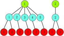
(a) CSF

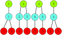
(b) B-CSF

Figure 2: Convergence curves of cuFasterTucker and its contrasting algorithm, they all set $J_{n}=32,n\in\{N\}$ and $R=32$.

IV-B Worker Parallelization

GPU is a single-instruction multi-device architecture that can execute multiple blocks in parallel, and a block contains multiple threads. Multiple threads form a thread group, and the size of the scheduling unit (Warp) of the current mainstream Nvidia GPU architecture is $32$ threads. Therefore, it has better performance when the number of threads in a thread block is a divisor or multiple of $32$, and the number of threads in a block is a multiple of $32$. We divide each block into multiple thread groups and treat a thread group as a worker. Each worker is responsible for a sub-tensor of tensor $\mathcal{X}$ at a time, and this sub-tensor is obtained by fixing a certain index of a certain dimension of tensor $\mathcal{X}$. We use the B-CSF format to store the tensor $\mathcal{X}$, which makes the number of non-zero elements contained in each sub-tensor relatively balanced. Therefore, the loads of multiple thread groups in multiple blocks are not much different, which avoids the problem of very unbalanced load among thread groups.

IV-C Thread Parallelization

Although each worker is responsible for a sub-tensor, instead of processing multiple non-zero elements at the same time, all non-zero elements of the sub-tensor are sequentially traversed. If a single threads group updates multiple non-zero elements at the same time, it will bring new load balancing problems, multiple calculations of intermediate variables, and additional communication overhead. We make each thread in the thread group process a scalar, then a threads group can process a vector. We set all $J_{n},n\in\{N\}$ to be divisors of $32$ or multiples of $32$. If $J_{n},n\in\{N\}$ is a divisor of $32$ including $32$, set the size of the thread group to $J_{n},n\in\{N\}$. A thread group processes exactly one vector of length $J_{n},n\in\{N\}$, the size of $\textbf{a}^{(n)}_{i_{n}},n\in\{N\}$ or $\textbf{b}^{(n)}_{:,r},n\in\{N\},r\in\{R\}$, at a time. If $J_{n},n\in\{N\}$ is a multiple of $32$ excluding $32$, set the thread group size to $32$. A thread group processes a vector of length $32$ at a time, the thread group processes multiple times to complete the processing of a vector of length $J_{n},n\in\{N\}$.

IV-D Fine-grained Parallelization

According to the algorithmic characteristics of the Fastertucker and the architectural characteristics of the GPU, we perform fine-grained parallel optimization on the proposed cuFasterTucker. The major optimization techniques in cuFasterTucker are concluded as:

$\mathcal{G}\{parameter\}$: parameter in global memory.

$\mathcal{C}\{parameter\}$: parameter in on-chip cache memory.

$\mathcal{R}\{parameter\}$: parameter in register memory.

Input: Initialized factor matrices $\textbf{A}^{(n)}$ $\in$ $\mathbb{R}^{I_{n}\times J_{n}}$, $n\in\{N\}$ and core matrices $\textbf{B}^{(n)}$ $\in$ $\mathbb{R}^{J_{n}\times R}$, $n\in\{N\}$.

Output: Reusable intermediate variables $\textbf{a}^{(n)}_{i_{n}}\textbf{b}^{(n)}_{:,r},n\in\{N\},r\in\{R\}$.

1:  for $n$ from $1$ to $N$ do

2:     for $r$ from $1$ to $R$ do

3:        $\mathcal{C}\{\textbf{b}^{(n)}_{:,r}\}$ $\leftarrow$ $\mathcal{G}\{\textbf{b}^{(n)}_{:,r}\}$

4:     end for

5:     for $i_{n}$ from $1$ to $I_{n}$ (Worker Parallelization) do

6:        $\mathcal{R}\{\textbf{a}^{(n)}_{i_{n}}\}$ $\leftarrow$ $\mathcal{G}\{\textbf{a}^{(n)}_{i_{n}}\}$

7:        for $r$ from $1$ to $R$ do

8:           $\mathcal{G}\{\textbf{a}^{(n)}_{i_{n}}\textbf{b}^{(n)}_{:,r}\}$ $\leftarrow$ $\mathcal{R}\{\textbf{a}^{(n)}_{i_{n}}\}$ $\cdot$ $\mathcal{C}\{\textbf{b}^{(n)}_{:,r}\}$

9:        end for

10:     end for

11:  end for

Algorithm 3 The calculation and storage of the reusable intermediate variables

Memory Coalescing: The GPU’s global memory is implemented with Dynamic Random Access Memory (DRAM), but DRAM is slow. Based on the parallelism of DRAM, we can achieve higher global memory access efficiency by optimizing the memory access pattern of threads, namely the Memory Coalescing technique. Memory Coalescing takes advantage of the fact that at any given point in time, threads in a warp are executing the same instructions, then optimal memory pattern will be achieved when all threads in a warp access global memory locations contiguously access mode. According to the algorithm characteristics of cuFasterTucker, all the variable matrices $\textbf{A}^{(n)}$ $\in$ $\mathbb{R}^{I_{n}\times J_{n}}$, $n$ $\in$ $\{N\}$ and $\textbf{B}^{(n)}$ $\in$ $\mathbb{R}^{J_{n}\times R}$, $n$ $\in$ $\{N\}$ are stored as the form of $\textbf{A}^{(n)}$ $\in$ $\mathbb{R}^{I_{n}\times J_{n}}$, $n$ $\in$ $\{N\}$ and $\textbf{B}^{(n)^{T}}$ $\in$ $\mathbb{R}^{R\times J_{n}}$, $n$ $\in$ $\{N\}$ to ensure that consecutive threads access consecutive memory addresses.

$\mathcal{G}\{parameter\}$: parameter in global memory.

$\mathcal{C}\{parameter\}$: parameter in on-chip cache memory.

$\mathcal{R}\{parameter\}$: parameter in register memory.

Input: Sparse tensor $\mathcal{X}$ $\in$ $\mathbb{R}^{I_{1}\times\cdots\times I_{N}}$, initialized factor matrices $\textbf{A}^{(n)}$ $\in$ $\mathbb{R}^{I_{n}\times J_{n}}$, $n\in\{N\}$ and core matrices $\textbf{B}^{(n)}$ $\in$ $\mathbb{R}^{J_{n}\times R}$, $n\in\{N\}$, reusable intermediate variables $\textbf{a}^{(n)}_{i_{n}}\textbf{b}^{(n)}_{:,r},n\in\{N\},r\in\{R\}$, learning rate $\gamma_{\textbf{A}}$, regularization parameter $\lambda_{\textbf{A}}$.

Output: Factor matrices $\textbf{A}^{(n)}$, $n$ $\in$ $\{N\}$.

1:  for $n$ from $1$ to $N$ do

2:     for $i_{n}$ from $1$ to $I^{{}^{\prime}}_{n}$ (Worker Parallelization) do

3:        for $r$ from $1$ to $R$ do

4:           $\mathcal{C}\{\textbf{b}^{(n)}_{:,r}\}$ $\leftarrow$ $\mathcal{G}\{\textbf{b}^{(n)}_{:,r}\}$

5:        end for

6:        for preorder traversal of subtensor $\mathcal{X}^{{}^{\prime}}_{i_{n}}$ do

7:           $d$ $=$ the depth of the subtensor $\mathcal{X}^{{}^{\prime}}_{i_{n}}$.

8:           $n^{{}^{\prime}}$ $=$ $(n+d)\%n$.

9:           if $d$ $=$ $N-1$ then

10:              $\mathcal{R}\{x_{i_{1},\dots,i_{n^{{}^{\prime}}},\dots,i_{N}}\}$ $\leftarrow$ $\mathcal{G}\{x_{i_{1},\dots,i_{n^{{}^{\prime}}},\dots,i_{N}}\}$ $-$ $\mathcal{G}\{\textbf{a}^{(n^{{}^{\prime}})}_{i_{n^{{}^{\prime}}}}\}$ $\cdot$ $\mathcal{R}\{\textbf{B}^{(n)}\textbf{Q}^{(n)^{T}}\textbf{s}^{(n)^{T}}_{i_{1},\dots,i_{N}}\}$

11:              $\mathcal{G}\{\textbf{a}^{(n^{{}^{\prime}})}_{i_{n^{{}^{\prime}}}}\}$ $\leftarrow$ $\mathcal{G}\{\textbf{a}^{(n^{{}^{\prime}})}_{i_{n^{{}^{\prime}}}}\}$ $-$ $\gamma_{\textbf{A}}$ $\cdot$ $\big{(}$ $\mathcal{R}\{x_{i_{1},\dots,i_{n^{{}^{\prime}}},\dots,i_{N}}\}$ $\cdot$ $\mathcal{G}\{\textbf{a}^{(n^{{}^{\prime}})}_{i_{n^{{}^{\prime}}}}\}$ $\cdot$ $\mathcal{R}\{\textbf{B}^{(n)}\textbf{Q}^{(n)^{T}}\textbf{s}^{(n)^{T}}_{i_{1},\dots,i_{N}}\}$ $+$ $\lambda_{\textbf{A}}$ $\cdot$ $\mathcal{G}\{\textbf{a}^{(n^{{}^{\prime}})}_{i_{n^{{}^{\prime}}}}\}$ $\big{)}$

12:           else if $d$ $=$ $N-2$ then

13:              $\mathcal{R}\{\textbf{B}^{(n)}\textbf{Q}^{(n)^{T}}\textbf{s}^{(n)^{T}}_{i_{1},\dots,i_{N}}\}$ $\leftarrow$ $0$

14:              for $r$ from $1$ to $R$ do

15:                 $\mathcal{R}\{\textbf{b}^{(n)}_{:,r}\textbf{s}^{(n)}_{i_{1},\dots,i_{N}}\textbf{q}^{(n)}_{:,r}\}$ $\leftarrow$ $\mathcal{C}\{\textbf{b}^{(n)}_{:,r}\}$

16:                 for $n^{{}^{\prime\prime}}$ from $1$ to $N$, $n^{{}^{\prime\prime}}$ $\neq$ $(n+N-1)\%n$ do

17:                    $\mathcal{R}\{\textbf{b}^{(n)}_{:,r}\textbf{s}^{(n)}_{i_{1},\dots,i_{N}}\textbf{q}^{(n)}_{:,r}\}$ $\leftarrow$ $\mathcal{R}\{\textbf{b}^{(n)}_{:,r}\textbf{s}^{(n)}_{i_{1},\dots,i_{N}}\textbf{q}^{(n)}_{:,r}\}$ $\cdot$ $\mathcal{C}\{\textbf{a}^{(n^{{}^{\prime\prime}})}_{i_{n^{{}^{\prime\prime}}}}\textbf{b}^{(n^{{}^{\prime\prime}})}_{:,r}\}$

18:                 end for

19:                 $\mathcal{R}\{\textbf{B}^{(n)}\textbf{Q}^{(n)^{T}}\textbf{s}^{(n)^{T}}_{i_{1},\dots,i_{N}}\}$ $\leftarrow$ $\mathcal{R}\{\textbf{B}^{(n)}\textbf{Q}^{(n)^{T}}\textbf{s}^{(n)^{T}}_{i_{1},\dots,i_{N}}\}$ $+$ $\mathcal{R}\{\textbf{b}^{(n)}_{:,r}\textbf{s}^{(n)}_{i_{1},\dots,i_{N}}\textbf{q}^{(n)}_{:,r}\}$

20:              end for

21:           else

22:              for $r$ from $1$ to $R$ do

23:                 $\mathcal{C}\{\textbf{a}^{(n^{{}^{\prime}})}_{i_{n}^{{}^{\prime}}}\textbf{b}^{(n^{{}^{\prime}})}_{:,r}\}$ $\leftarrow$ $\mathcal{G}\{\textbf{a}^{(n^{{}^{\prime}})}_{i_{n}}\textbf{b}^{(n^{{}^{\prime}})}_{:,r}\}$

24:              end for

25:           end if

26:        end for

27:     end for

28:  end for

Algorithm 4 Update factor matrices in cuFasterTucker

Warp Shuffle: The warp shuffle instructions allows a thread to directly read the register values of other threads, as long as these threads are in the same warp. It is implemented through additional hardware support, which is better than shared memory for inter-thread communication, has lower latency, and does not consume additional memory resources to perform data exchange. The warp shuffle instructions is commonly used to calculate dot product and sum in scientific computing, in cuFasterTucker we use to calculate $\textbf{a}^{(n)}_{i_{n}}\cdot\textbf{b}^{(n)}_{:,r},i_{n}\in\{I_{n}\},n\in\{N\},r\in\{R\}$ and $\textbf{a}^{(n)}_{i_{n}}\cdot\textbf{B}^{(n)}\textbf{Q}^{(n)^{T}}\textbf{s}^{(n)^{T}}_{i_{1},\dots,i_{N}},i_{n}\in\{I_{n}\},n\in\{N\}$.

On-chip Cache: The current mainstream architecture of NVIDIA NGPU allows programmatic control over the caching behavior of the on-chip L1 cache. In cuFasterTucker, we use $\_\_ldg$ to put predictably reusable intermediate variables and commonly used variables into the on-chip L1 cache to improve memory access efficiency, such as $\textbf{a}^{(n)}_{i_{n}}\textbf{b}^{(n)}_{:,r},i_{n}\in\{I_{n}\},n\in\{N\},r\in\{R\}$ and $\textbf{b}^{(n)}_{:,r},n\in\{N\},r\in\{R\}$ stored in global memory. In practice, the GPU’s cache scheduling also works well.

Shared Memory: In the current mainstream architecture of nvidia gpus, shared memory is put into the on-chip L1 cache, which is much faster than global memory. At the same time registers on the gpu are not suitable for storing contiguous vectors. Therefore cuFasterTucker uses shared memory to store reusable intermediate vectors and use them for the next process. In the update core matrices module, we use shared memory to store $\textbf{s}^{(n)}_{i_{1},\dots,i_{N}}\textbf{q}^{(n)}_{:,r},n\in\{N\},r\in\{R\}$.

Register: The storage structure of each variable of cuFasterTucker is clearly allocated, and all variables occupy only a small amount of storage space, that is, the registers in the gpu are completely sufficient for cuFasterTucker. Due to the structure of B-CSF, the index and value of tensor $\mathcal{X}$ are read and put into registers for the next process without re-reading from global memory. In addition, a register of each thread can store a scalar, and a thread group can store a vector. The premise of such storage is that each thread is only responsible for reading, writing and computing its own registers. In cuFasterTucker, vectors $\textbf{a}^{(n)}_{i_{n}},i_{n}\in\{I_{n}\},n\in\{N\}$ and $\textbf{B}^{(n)}\textbf{Q}^{(n)^{T}}\textbf{s}^{(n)^{T}}_{i_{1},\dots,i_{N}},n\in\{N\}$ are all stored in registers in this form.

IV-E Overview

cuFasterTucker is mainly composed of three parts, the first part is the calculation and storage of the reusable intermediate variables $\textbf{a}^{(n)}_{i_{n}}\textbf{b}^{(n)}_{:,r},n\in\{N\},r\in\{R\}$, the second part is the update factor matrices, and the third part is the update core matrices. Updating the factor matrices and updating the core matrices can be performed independently or simultaneously. But before that, the reusable intermediate variable $\textbf{a}^{(n)}_{i_{n}}\textbf{b}^{(n)}_{:,r},n\in\{N\},r\in\{R\}$ must be computed and stored. We use three algorithms to separately describe in detail how these three parts are implemented in parallel on the GPU. The worker parallelization in the algorithms has been marked, and each process is thread parallelization.

Algorithm 3 describes the process of computing and storing $\textbf{a}^{(n)}_{i_{n}}\cdot\textbf{b}^{(n)}_{:,r},i_{n}\in\{I_{n}\},n\in\{N\},r\in\{R\}$. For each order $n$, the repeatedly used $\textbf{b}^{(n)}_{:,r},r\in\{R\}$ is placed in the on-chip cache at first to improve the memory access efficiency during the calculation process (Algorithm 3, Line 3). Next, multiple workers process $\textbf{a}^{(n)}_{i_{n}},i_{n}\in\{I_{n}\}$ in parallel and put $\textbf{a}^{(n)}_{i_{n}}$ into registers to improve the memory access efficiency of $\textbf{a}^{(n)}_{i_{n}}$ for the next calculation of $\textbf{a}^{(n)}_{i_{n}}\cdot\textbf{b}^{(n)}_{:,r},r\in\{R\}$ (Algorithm 3, Line 6). Finally, the calculated $\textbf{a}^{(n)}_{i_{n}}\cdot\textbf{b}^{(n)}_{:,r},i_{n}\in\{I_{n}\},r\in\{R\}$ is stored in global memory for use when updating the factor matrices or core matrices (Algorithm 3, Line 8).

$\mathcal{G}\{parameter\}$: parameter in global memory.

$\mathcal{C}\{parameter\}$: parameter in on-chip cache memory.

$\mathcal{S}\{parameter\}$: parameter in shared memory.

$\mathcal{R}\{parameter\}$: parameter in register memory.

Input: Sparse tensor $\mathcal{X}$ $\in$ $\mathbb{R}^{I_{1}\times\cdots\times I_{N}}$, initialized factor matrices $\textbf{A}^{(n)}$ $\in$ $\mathbb{R}^{I_{n}\times J_{n}}$, $n\in\{N\}$ and core matrices $\textbf{B}^{(n)}$ $\in$ $\mathbb{R}^{J_{n}\times R}$, $n\in\{N\}$, learning rate $\gamma_{\textbf{B}}$, regularization parameter $\lambda_{\textbf{B}}$.

Output: Core matrices $\textbf{B}^{(n)}$, $n$ $\in$ $\{N\}$.

1:  for $n$ from $1$ to $N$ do

2:     for $r$ from $1$ to $R$ do

3:        $\mathcal{G}\{$ $The$ $gradient$ $of$ $\textbf{b}^{(n)}_{:,r}\}$ $\leftarrow$ $0$

4:     end for

5:     for $i_{n}$ from $1$ to $I^{{}^{\prime}}_{n}$ (Worker Parallelization) do

6:        for $r$ from $1$ to $R$ do

7:           $\mathcal{C}\{\textbf{b}^{(n)}_{:,r}\}$ $\leftarrow$ $\mathcal{G}\{\textbf{b}^{(n)}_{:,r}\}$

8:        end for

9:        for preorder traversal of subtensor $\mathcal{X}^{{}^{\prime}}_{i_{n}}$ do

10:           $d$ $=$ the depth of the subtensor $\mathcal{X}^{{}^{\prime}}_{i_{n}}$.

11:           $n^{{}^{\prime}}$ $=$ $(n+d)\%n$.

12:           if $d$ $=$ $N-1$ then

13:              $\mathcal{R}\{x_{i_{1},\dots,i_{n^{{}^{\prime}}},\dots,i_{N}}\}$ $\leftarrow$ $\mathcal{G}\{x_{i_{1},\dots,i_{n^{{}^{\prime}}},\dots,i_{N}}\}$ $-$ $\mathcal{G}\{\textbf{a}^{(n^{{}^{\prime}})}_{i_{n^{{}^{\prime}}}}\}$ $\cdot$ $\mathcal{R}\{\textbf{B}^{(n)}\textbf{Q}^{(n)^{T}}\textbf{s}^{(n)^{T}}_{i_{1},\dots,i_{N}}\}$

14:              for $r$ from $1$ to $R$ do

15:                 $\mathcal{G}\{$ $The$ $gradient$ $of$ $\textbf{b}^{(n)}_{:,r}\}$ $\leftarrow$ $\mathcal{G}\{$ $The$ $gradient$ $of$ $\textbf{b}^{(n)}_{:,r}\}$ $+$ $\mathcal{R}\{x_{i_{1},\dots,i_{n^{{}^{\prime}}},\dots,i_{N}}\}$ $\cdot$ $\mathcal{G}\{\textbf{a}^{(n^{{}^{\prime}})}_{i_{n^{{}^{\prime}}}}\}$ $\cdot$ $\mathcal{S}\{\textbf{s}^{(n)}_{i_{1},\dots,i_{N}}\textbf{q}^{(n)}_{:,r}\}$

16:              end for

17:           else if $d$ $=$ $N-2$ then

18:              $\mathcal{R}\{\textbf{B}^{(n)}\textbf{Q}^{(n)^{T}}\textbf{s}^{(n)^{T}}_{i_{1},\dots,i_{N}}\}$ $\leftarrow$ $0$

19:              for $r$ from $1$ to $R$ do

20:                 $\mathcal{S}\{\textbf{s}^{(n)}_{i_{1},\dots,i_{N}}\textbf{q}^{(n)}_{:,r}\}$ $\leftarrow$ $1.0$

21:                 for $n^{{}^{\prime\prime}}$ from $1$ to $N$, $n^{{}^{\prime\prime}}$ $\neq$ $(n+N-1)\%n$ do

22:                    $\mathcal{S}\{\textbf{s}^{(n)}_{i_{1},\dots,i_{N}}\textbf{q}^{(n)}_{:,r}\}$ $\leftarrow$ $\mathcal{S}\{\textbf{s}^{(n)}_{i_{1},\dots,i_{N}}\textbf{q}^{(n)}_{:,r}\}$ $\cdot$ $\mathcal{C}\{\textbf{a}^{(n^{{}^{\prime\prime}})}_{i_{n^{{}^{\prime\prime}}}}\textbf{b}^{(n^{{}^{\prime\prime}})}_{:,r}\}$

23:                 end for

24:                 $\mathcal{R}\{\textbf{B}^{(n)}\textbf{Q}^{(n)^{T}}\textbf{s}^{(n)^{T}}_{i_{1},\dots,i_{N}}\}$ $\leftarrow$ $\mathcal{R}\{\textbf{B}^{(n)}\textbf{Q}^{(n)^{T}}\textbf{s}^{(n)^{T}}_{i_{1},\dots,i_{N}}\}$ $+$ $\mathcal{S}\{\textbf{s}^{(n)}_{i_{1},\dots,i_{N}}\textbf{q}^{(n)}_{:,r}\}$ $\cdot$ $\mathcal{C}\{\textbf{b}^{(n)}_{:,r}\}$

25:              end for

26:           else

27:              for $r$ from $1$ to $R$ do

28:                 $\mathcal{C}\{\textbf{a}^{(n^{{}^{\prime}})}_{i_{n}}\textbf{b}^{(n^{{}^{\prime}})}_{:,r}\}$ $\leftarrow$ $\mathcal{G}\{\textbf{a}^{(n^{{}^{\prime}})}_{i_{n}}\textbf{b}^{(n^{{}^{\prime}})}_{:,r}\}$

29:              end for

30:           end if

31:        end for

32:     end for

33:     for $r$ from $1$ to $R$ do

34:        $\mathcal{G}\{\textbf{b}^{(n)}_{:,r}\}$ $\leftarrow$ $\mathcal{G}\{\textbf{b}^{(n)}_{:,r}\}$ $-$ $\gamma_{\textbf{B}}$ $\cdot$ $\big{(}$ $\mathcal{G}\{$ $The$ $gradient$ $of$ $\textbf{b}^{(n)}_{:,r}\}$ $/$ $|\Omega|$ $+$ $\lambda_{\textbf{B}}$ $\cdot$ $\mathcal{G}\{\textbf{b}^{(n)}_{:,r}\}$ $\big{)}$

35:     end for

36:  end for

Algorithm 5 Update core matrices in cuFasterTucker

Algorithm 4 describes the process of updating $\textbf{a}^{(n)}_{i_{n}},i_{n}\in\{I_{n}\},n\in\{N\}$. For each order $n$, multiple workers process $I^{{}^{\prime}}_{n}$ sub-tensors $\mathcal{X}^{{}^{\prime}}_{i_{n}}$ in parallel (Algorithm 4, line 2). The repeatedly used $\textbf{b}^{(n)}_{:,r},r\in\{R\}$ is placed in the on-chip cache at first to improve the memory access efficiency during the calculation process (Algorithm 4, line 4). Next, each subtensor $\mathcal{X}^{{}^{\prime}}_{i_{n}}$ is preorder traversed by a worker (Algorithm 4, line 6). If the node is not a leaf node or the parent node of the leaf node (Algorithm 4, line 21), the corresponding intermediate variable $\textbf{a}^{(n^{{}^{\prime}})}_{i_{n}^{{}^{\prime}}}\textbf{b}^{(n^{{}^{\prime}})}_{:,r}$ is put into the on-chip cache (Algorithm 4, line 23), which provides memory access acceleration for the subsequent computation. If the node is the parent node of the leaf node (Algorithm 4, line 12), the shared intermediate variable $\textbf{B}^{(n)}\textbf{Q}^{(n)^{T}}\textbf{s}^{(n)^{T}}_{i_{1},\dots,i_{N}}$ is calculated and put into the register (Algorithm 4, lines 13-20). If the node is a leaf node (Algorithm 4, line 9), the corresponding $\textbf{a}^{(n^{{}^{\prime}})}_{i_{n^{{}^{\prime}}}}$ is updated (Algorithm 4, lines 10-11). Each time a order is processed, $\textbf{a}^{(n)}_{i_{n}}\textbf{b}^{(n)}_{:,r},n\in\{N\},r\in\{R\}$ in global memory needs to be updated (Algorithm 3, Lines 2-10). Note that since the B-CSF tensor storage format is used, when dealing with the $n$th order, $\textbf{a}^{(n)}_{i_{n}}\textbf{b}^{(n)}_{:,r},n=(n+N-1)\%n,i_{n}\in\{I_{n}\},r\in\{R\}$ is updated.

Algorithm 5 describes the process of updating $\textbf{b}^{(n)}_{:,r},n\in\{N\},r\in\{R\}$. Since the core matrices is required by all workers, and the scale of the core matrices in practical applications is usually small, it is not suitable to update the core matrices in parallel in real time. We accumulate the gradients of each set of non-zero elements and update the core matrices uniformly at the end. For each order $n$, store the gradient of $\textbf{b}^{(n)}_{:,r}\},r\in\{R\}$ in global memory at first (Algorithm 5, line 3). Next, multiple workers process $I^{{}^{\prime}}_{n}$ sub-tensors $\mathcal{X}^{{}^{\prime}}_{i_{n}}$ in parallel (Algorithm 5, line 5). Then, the repeatedly used $\textbf{b}^{(n)}_{:,r},r\in\{R\}$ is placed in the on-chip cache to improve the memory access efficiency during the calculation process (Algorithm 5, line 7). Each subtensor $\mathcal{X}^{{}^{\prime}}_{i_{n}}$ is preorder traversed by a worker (Algorithm 5, line 9). If the node is not a leaf node or the parent node of the leaf node (Algorithm 5, line 26), the corresponding intermediate variable $\textbf{a}^{(n^{{}^{\prime}})}_{i_{n}^{{}^{\prime}}}\textbf{b}^{(n^{{}^{\prime}})}_{:,r}$ is put into the on-chip cache (Algorithm 5, lines 27-29), which provides memory access acceleration for the subsequent computation. If the node is the parent node of the leaf node (Algorithm 5, line 17), the shared intermediate variable $\textbf{s}^{(n)}_{i_{1},\dots,i_{N}}\textbf{q}^{(n)}_{:,r},r\in\{R\}$ is calculated and put into the shared memory (Algorithm 5, lines 18-25). If the node is a leaf node (Algorithm 5, line 12), the gradient of $\textbf{b}^{(n)}_{:,r}\},r\in\{R\}$ is computed and accumulated into global memory. After all gradients are accumulated, the $\textbf{b}^{(n)}_{:,r}\},r\in\{R\}$ updated (Algorithm 5, lines 13-16). Same as when updating factor matrices, each time a order is processed, $\textbf{a}^{(n)}_{i_{n}}\textbf{b}^{(n)}_{:,r},n\in\{N\},r\in\{R\}$ in global memory needs to be updated (Algorithm 3, Lines 2-10). And when dealing with the $n$th order, $\textbf{a}^{(n)}_{i_{n}}\textbf{b}^{(n)}_{:,r},n=(n+N-1)\%n,i_{n}\in\{I_{n}\},r\in\{R\}$ is updated.

V Experiments

We present experimental results to answer the following questions.

1. Time for a single iteration. How well does cuFasterTucker and its contrasting algorithms perform in terms of iteration speed? Is it the same efficiency for tensor storage format using COO or CSF? Does the extraction of reusable intermediate variables and shared invariant intermediate Variables improve the efficiency of the algorithm?

2. Real-world accuracy. How accurate do cuFasterTucker and its contrasting algorithms on real-world datasets?

3. Adaptability of high-order tensors. How well does cuFasterTucker and its contrasting algorithms perform on high-order datasets?

4. Adaptability of tensor sparsity. Does the sparsity of tensors have an effect on cufast and its contrasting algorithms?

We describe the datasets and experimental settings in Section V-A, and answer the questions in Sections V-B to V-E.

TABLE II: Real World Datasets

	Netflix	Yahoo!Music
$I_{1}$	480, 189	1, 000, 990
$I_{2}$	17, 770	624, 961
$I_{3}$	2, 182	3, 075
$|\Omega|$	99, 072, 112	250, 272, 286
$|\Gamma|$	1, 408, 395	2, 527, 989
Max Value	5	5
Min Value	1	0.025

TABLE III: Synthetic Datasets

	Synthetic(Order)	Synthetic(Sparsity)
$order$	3,4,5,6,7,8,9,10	3
$I$	10, 000	1, 000
$|\Omega|$	100M	20M,40M,60M,80M,100M
Max Value	5	5
Min Value	1	1

V-A Experimental Settings

1. Datasets: We use both real-world and synthetic datasets to evaluate cuFasterTucker and its contrasting algorithms. For real-world datasets, we use Netflix and Yahoo!music . Netflix is movie rating data which consist of (user, movie, time, rating). Yahoo!music is music rating data which consist of (user, music, time, rating). Using Netflix as the standard, we normalize all values of the Yahoo!music dataset between $0$ to $5$. For synthetic datasets, we create two kinds of random tensors. One contains $8$ tensors with orders from $3$ to $10$, while other parameters remain the same. These tensors are used to examine the performance of cuFasterTucker and its contrasting algorithms on high-order tensors. The other contains $5$ tensors with the number of non-zero elements ranging from $20$ million to $100$ million, and other parameters remain the same. Since we set the order to $3$ and the length of each order is $1000$, the sparsity of these tensors are $2\%$, $4\%$, $6\%$, $8\%$ and $10\%$ respectively. These tensors are used to examine the performance of cuFasterTucker and its contrasting algorithms on tensors of different sparsity. Tables II and III describe the real-world datasets and synthetic datasets used in the experiments, respectively.

2. Contrasting algorithms: We compare cuFasterTucker and its variants with the state-of-the-art FasterTucker factorization algorithm cuFastTucker and other parallel sparse Tucker decomposition algorithms. As far as we know, there is only one FastTucker factorization algorithm. Descriptions of all methods are given as follows:

   • P-Tucker[21]: A scalable Tucker decomposition method for sparse tensors.

   • Vest[22]: A tensor decomposition method for large partially observable data to output a very sparse core tensor and factor matrices.

   • SGD__Tucker[30]: A Novel Stochastic Optimization Strategy for Parallel Sparse Tucker Decomposition.

   • ParTi[23]: A fast essential sparse tensor operations and tensor decompositions method on multicore CPU and GPU architectures.

   • GTA[24]: A general framework for Tucker decomposition on heterogeneous platforms.

   • cuTucker[28]: A parallel sparse Tucker decomposition algorithm on the CUDA platform.

   • cuFastTucker[28]: A parallel sparse FastTucker decomposition algorithm on the CUDA platform with polynomial computational complexity.

   • cuFasterTucker_COO: A cuFastertucker algorithm, which only reduces the computation of reusable intermediate variables, uses the same tensor storage format COO as cuFastTucker.

   • cuFasterTucker_B-CSF: A cuFasterTucker algorithm, which only reduces the computation of reusable intermediate variables, uses B-CSF, a tensor storage format that is not identical to cuFastTucker.

   • cuFasterTucker: The complete cuFasterTucker algorithm, which reduces the computation of reusable intermediate variables and shared intermediate variables.

3. Environment: cuFasterTucker is implemented in C/C++ with CUDA. For its contrasting algorithm cuFastTucker, we use the original implementations provided by the authors. The experiments of P-Tucker, Vest and SGD__Tucker are ran on a Intel Core i7-12700K CPU with 64GB RAM. The experiments of ParTi, GTA, cuTucker, cuFastTucker, cuFasterTucker_COO, cuFasterTucker_B-CSF and cuFasterTucker are ran on a NVIDIA GeForce RTX 3080Ti GPU with 12GB graphic memory. We set the fiber threshold to $128$ for the B-CSF tensor storage format, which is considered to have the best performance. We set the maximum number of iterations to $50$ and report the average time for a single iteration.

V-B Time for a single iteration

We use real-world datasets to evaluate the running speed of cuFasterTucker and its contrasting algorithms, i.e. the time required for a single iteration. In order to facilitate contrasting and maximize algorithm efficiency, all algorithms take $J_{n}=32,n\in\{N\}$ and $R=32$. However, most of the advanced sparse Tucker decomposition algorithms can not adapt to the HOHDST. Table IV shows the single iteration time of these algorithms or the reason why they cannot work. We relax the conditions appropriately. When $J_{n}=16,n\in\{N\}$, it takes $4829.497819$ seconds and $10816.486406$ seconds for Vest to update the factor matrices on Netflix and Yahoo!Music datasets, respectively. And it takes $9492.699654$ seconds and $29746.486010$ seconds for Vest to update the core matrices on Netflix and Yahoo!Music datasets, respectively. When $J_{n}=8,n\in\{N\}$, ParTi can run on the Yahoo!Music dataset, and its single iteration time is $54.861532$ seconds. In addition, the preprocessing time of ParTi on Netflix and Yahoo!Music datasets is $249.978767$ seconds and $646.884534$ seconds respectively. When $J_{n}=16,n\in\{N\}$, GTA can run on the Netflix dataset, and the single iteration time is $243.797254$ seconds. And when $J_{n}=8,n\in\{N\}$, GTA can run on the Yahoo!Music dataset, and the single iteration time is $22.904287$ seconds. It can be seen that the above algorithms cannot meet our requirements for processing HOHDST.

TABLE IV: The single iteration time (seconds) or error of sparse Tucker decomposition algorithms

Algorithm	Netflix	Yahoo!Music
P-Tucker(Factor)	2886.727982	7381.461875
Vest(Factor)	out of time	out of time
SGD__Tucker(Factor)	609.306086	1354.774812
ParTi(Factor)	67.537985	out of memory
GTA(Factor)	out of memory	out of memory
cuTucker(Factor)	64.648387	163.867682
Vest(Core)	out of time	out of time
cuTucker(Core)	63.404410	161.934037

In Table V, the average time(seconds) for a single iteration of each sparse Fast Tucker decomposition algorithm are presented. Due to the storage and invocation of reusable intermediate variables, cuFasterTucker_COO achieves a speedup of more than $3.0X$ in updating factor matrices and updating core matrices compared to cuFastTucker. Compared with cuFasterTucker_COO, cuFasterTucker_B-CSF is only a tensor storage format change, but therefore cuFasterTucker_B-CSF has obtained a speedup of $2.0X$ to $5.0X$ relative to cuFastTucker in updating the factor matrices and the core matrices, respectively. However, compared with cuFasterTucker_B-CSF, there is a significant difference in the increase of the speedup ratio relative to cuFastTucker obtained by cuFasterTucker when updating the factor matrices and updating the core matrices. When updating the factor matrices, cuFasterTucker has a speedup growth of $7.0X$ to $8.0X$, while updating the core matrices is only about $1.0X$. This is because the proportion of shared intermediate variables when updating the factor matrices is much larger than updating the core matrices. In fact, cuFastTucker and cuFasterTucker can run $10$ times the size of the Netflix dataset in 12GB of graphic memory.

TABLE V: Speedup comparison on the baseline cuFastTucker

Algorithm	Netflix	Yahoo!Music
cuFastTucker(Factor)	4.558734	11.557935
cuFasterTucker_COO(Factor)	1.385437(3.29X)	3.536883(3.27X)
cuFasterTucker_B-CSF(Factor)	0.534161(8.53X)	1.322512(8.74X)
cuFasterTucker(Factor)	0.294704(15.47X)	0.787373(14.68X)
cuFastTucker(Core)	6.044708	15.405755
cuFasterTucker_COO(Core)	1.947172(3.10X)	4.976965(3.10X)
cuFasterTucker_B-CSF(Core)	0.998262(6.06X)	2.505620(6.15X)
cuFasterTucker(Core)	0.835289(7.24X)	2.187568(7.04X)

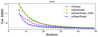
(a) RMSE on Netflix

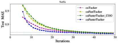
(b) MAE on Netflix

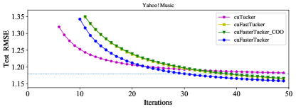
(c) RMSE on Yahoo!Music

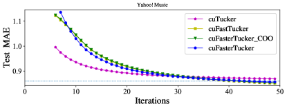
(d) MAE on Yahoo!Music

Figure 3: Convergence curves of cuFasterTucker and its contrasting algorithm, they all set $J_{n}=32,n\in\{N\}$ and $R=32$.

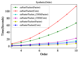
(a) Scalability on Synthesis Datasets

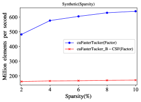
(b) Speedup on Netflix

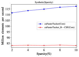
(c) Speedup on Yahoo!Music

Figure 4: (a) Adaptability of high-order tensors; (b)-(c) Adaptability of tensor sparsity.

V-C Real-world accuracy

We evaluate the accuracy of cuFasterTucker and its contrasting algorithms on the real-world datasets. The evaluation metrics are test Root Mean Square Error (RMSE) and test Mean Absolute Error(MAE) , which are widely used by recommender systems. We randomly generate factor matrices and core matrices, which follow an average distribution. Each algorithm iterates $50$ times and records the test RMSE and test MAE after each iteration. Figure 3 shows the convergence curves of cuFasterTucker and its contrasting algorithms. Figures 3(a) and 3(b) describe the changes of RMSE and MAE on the Netflix dataset, respectively, and Figures 3(c) and 3(d) describe the changes of rmse and mae on the Yahoo!Music dataset, respectively. It can be seen from Figure 3 that the above algorithms all converge within acceptable accuracy. The convergence curves of cuFasterTucker_COO and cuFastTucker almost coincide, which is predictable, because the difference between the two is only reflected in the amount of calculation and other update methods are consistent. cuFasterTucker converges a bit faster due to the data locality sensitivity of the B-CSF tensor storage format.

V-D Adaptability of high-order tensors

We use synthetic datasets Synthetic(Order) to examine the adaptability of cuFasterTucker and its contrasting algorithms for high-order tensors. The orders of these tensors range from $3$ to $10$, the length of each order is fixed at $1000$, and the number of non-zero elements is fixed at $100$ million. We set $J_{n}=32,n\in\{N\}$ and $R=32$ for all algorithms and recorded the average time(seconds) for a single iteration. Figure 4(a) shows the growth trend of the average single iteration time of these algorithms as the dimensionality increases. Both cuFasterTucker_COO and cuFasterTucker grow more slowly than cuFastTucker, depending on the computational complexity of the first two is much smaller than cuFastTucker. It can be seen that cuFasterTucker is more suitable for high-order FastTucker decomposition than cuFastTucker.

V-E Adaptability of tensor sparsity

We use synthetic datasets Synthetic(Sparsity) to examine the adaptability of cuFasterTucker and its contrasting algorithms to tensors of varying sparsity. The non-zero elements of these tensors range from $20$ million to $100$ million in increments of $20$ million, the order is fixed at $3$, and the length of each order is fixed at $1000$. That is, five tensors with a sparsity of 2% to 10% whose growth is 2%. Since the number of non-zero elements in each tensor is not the same, it is not appropriate for us to use the average time of a single iteration for comparison. We use the number of non-zero elements processed per second for comparison here. Figures 4(b) and 4(c) show the efficiency of cuFasterTucker and its contrasting algorithms for different sparsity in updating factor and core matrices, respectively. It can be seen that the efficiency of cuFasterTucker increases significantly with the increase of sparsity, while the efficiency of cuFasterTucker_B-CSF does not change significantly. As the data size increases, the amount of computation increases accordingly, and the sparsity increases, but the shared intermediate variables that cuFasterTucker needs to compute increases only slightly or even at all. The results show that cuFasterTucker is more friendly to tensors with high sparsity, but its performance on tensors with low sparsity is not worse than other algorithms.

VI Conclusion

We propose the FasterTucker algorithm, which has lower computational complexity than FastTucker and is more suitable for processing HOHDST. And we present a fine-grained parallel FasterTucker algorithm cuFasterTucker on GPU. cuFasterTucker uses the SGD method to sequentially update the factor matrix or core matrix of each order to achieve convergence. And cuFasterTucker uses the B-CSF tensor storage format to greatly improve the read and write efficiency during the update process while ensuring load balancing. cuFasterTucker is about $14$ times and $6$ times faster than existing state-of-the-art algorithms in updating factor matrices and core matrices, respectively. And the convergence speed is slightly improved. More importantly, compared with the current state-of-the-art algorithms, cuFasterTucker performs well on high-order tensors, and the single iteration time is much smaller than the former, and the higher the order, the more obvious the gap. Finally, cuFasterTucker performs better on denser tensors, a property that state-of-the-art algorithms do not have. In future work, we will explore the FastTucker algorithm with faster convergence speed and extend it to new parallel hardware platforms as well as distributed platforms.

References

• [1] T. G. Kolda and B. W. Bader, “Tensor decompositions and applications,” SIAM review, vol. 51, no. 3, pp. 455–500, 2009.
• [2] S. Ahmadi-Asl, S. Abukhovich, M. G. Asante-Mensah, A. Cichocki, A. H. Phan, T. Tanaka, and I. Oseledets, “Randomized algorithms for computation of tucker decomposition and higher order svd (hosvd),” IEEE Access, vol. 9, pp. 28 684–28 706, 2021.
• [3] Z. Chen, Z. Xu, and D. Wang, “Deep transfer tensor decomposition with orthogonal constraint for recommender systems,” in Proceedings of the AAAI Conference on Artificial Intelligence, vol. 35, no. 5, 2021, pp. 4010–4018.
• [4] S. Fernandes, H. Fanaee-T, and J. Gama, “Tensor decomposition for analysing time-evolving social networks: An overview,” Artificial Intelligence Review, vol. 54, no. 4, pp. 2891–2916, 2021.
• [5] P. Díez, S. Zlotnik, A. García-González, and A. Huerta, “Algebraic pgd for tensor separation and compression: an algorithmic approach,” Comptes Rendus Mécanique, vol. 346, no. 7, pp. 501–514, 2018.
• [6] F. Huang, X. Yue, Z. Xiong, Z. Yu, S. Liu, and W. Zhang, “Tensor decomposition with relational constraints for predicting multiple types of microrna-disease associations,” Briefings in bioinformatics, vol. 22, no. 3, p. bbaa140, 2021.
• [7] A.-H. Phan, P. Tichavskỳ, and A. Cichocki, “Error preserving correction: A method for cp decomposition at a target error bound,” IEEE Transactions on Signal Processing, vol. 67, no. 5, pp. 1175–1190, 2018.
• [8] Y. Shin and S. S. Woo, “Passwordtensor: Analyzing and explaining password strength using tensor decomposition,” Computers & Security, vol. 116, p. 102634, 2022.
• [9] H. Chen, F. Ahmad, S. Vorobyov, and F. Porikli, “Tensor decompositions in wireless communications and mimo radar,” IEEE Journal of Selected Topics in Signal Processing, vol. 15, no. 3, pp. 438–453, 2021.
• [10] M. Yin, Y. Sui, S. Liao, and B. Yuan, “Towards efficient tensor decomposition-based dnn model compression with optimization framework,” in Proceedings of the IEEE/CVF Conference on Computer Vision and Pattern Recognition, 2021, pp. 10 674–10 683.
• [11] R. K. Kaliyar, A. Goswami, and P. Narang, “Deepfake: improving fake news detection using tensor decomposition-based deep neural network,” The Journal of Supercomputing, vol. 77, no. 2, pp. 1015–1037, 2021.
• [12] E. E. Tyrtyshnikov, “Tensor decompositions and rank increment conjecture,” Russian Journal of Numerical Analysis and Mathematical Modelling, vol. 35, no. 4, pp. 239–246, 2020.
• [13] L. R. Tucker et al., “The extension of factor analysis to three-dimensional matrices,” Contributions to mathematical psychology, vol. 110119, 1964.
• [14] L. De Lathauwer, B. De Moor, and J. Vandewalle, “A multilinear singular value decomposition,” SIAM journal on Matrix Analysis and Applications, vol. 21, no. 4, pp. 1253–1278, 2000.
• [15] ——, “On the best rank-1 and rank-(r 1, r 2,…, r n) approximation of higher-order tensors,” SIAM journal on Matrix Analysis and Applications, vol. 21, no. 4, pp. 1324–1342, 2000.
• [16] U. Kang, E. Papalexakis, A. Harpale, and C. Faloutsos, “Gigatensor: scaling tensor analysis up by 100 times-algorithms and discoveries,” in Proceedings of the 18th ACM SIGKDD international conference on Knowledge discovery and data mining, 2012, pp. 316–324.
• [17] M. Haardt, F. Roemer, and G. Del Galdo, “Higher-order svd-based subspace estimation to improve the parameter estimation accuracy in multidimensional harmonic retrieval problems,” IEEE Transactions on Signal Processing, vol. 56, no. 7, pp. 3198–3213, 2008.
• [18] E. R. Balda, S. A. Cheema, J. Steinwandt, M. Haardt, A. Weiss, and A. Yeredor, “First-order perturbation analysis of low-rank tensor approximations based on the truncated hosvd,” in 2016 50th Asilomar Conference on Signals, Systems and Computers.   IEEE, 2016, pp. 1723–1727.
• [19] N. Vannieuwenhoven, R. Vandebril, and K. Meerbergen, “A new truncation strategy for the higher-order singular value decomposition,” SIAM Journal on Scientific Computing, vol. 34, no. 2, pp. A1027–A1052, 2012.
• [20] L. Grasedyck, “Hierarchical singular value decomposition of tensors,” SIAM journal on matrix analysis and applications, vol. 31, no. 4, pp. 2029–2054, 2010.
• [21] S. Oh, N. Park, S. Lee, and U. Kang, “Scalable tucker factorization for sparse tensors-algorithms and discoveries,” in 2018 IEEE 34th International Conference on Data Engineering (ICDE).   IEEE, 2018, pp. 1120–1131.
• [22] M. Park, J.-G. Jang, and L. Sael, “Vest: Very sparse tucker factorization of large-scale tensors,” in 2021 IEEE International Conference on Big Data and Smart Computing (BigComp).   IEEE, 2021, pp. 172–179.
• [23] J. Li, Y. Ma, and R. Vuduc, “ParTI! : A parallel tensor infrastructure for multicore cpus and gpus,” Oct 2018, last updated: Jan 2020. [Online]. Available: http://parti-project.org
• [24] S. Oh, N. Park, J.-G. Jang, L. Sael, and U. Kang, “High-performance tucker factorization on heterogeneous platforms,” IEEE Transactions on Parallel and Distributed Systems, vol. 30, no. 10, pp. 2237–2248, 2019.
• [25] V. N. Ioannidis, A. S. Zamzam, G. B. Giannakis, and N. D. Sidiropoulos, “Coupled graphs and tensor factorization for recommender systems and community detection,” IEEE Transactions on Knowledge and Data Engineering, vol. 33, no. 3, pp. 909–920, 2019.
• [26] T. Cheng, J. Wen, Q. Xiong, J. Zeng, W. Zhou, and X. Cai, “Personalized web service recommendation based on qos prediction and hierarchical tensor decomposition,” IEEE Access, vol. 7, pp. 62 221–62 230, 2019.
• [27] P. Wang, L. T. Yang, G. Qian, J. Li, and Z. Yan, “Ho-otsvd: A novel tensor decomposition and its incremental decomposition for cyber–physical–social networks (cpsn),” IEEE Transactions on Network Science and Engineering, vol. 7, no. 2, pp. 713–725, 2019.
• [28] Z. Li, “cu_fasttucker: A faster and stabler stochastic optimization for parallel sparse tucker decomposition on multi-gpus,” arXiv preprint arXiv:2204.07104, 2022.
• [29] I. Nisa, J. Li, A. Sukumaran-Rajam, R. Vuduc, and P. Sadayappan, “Load-balanced sparse mttkrp on gpus,” in 2019 IEEE International Parallel and Distributed Processing Symposium (IPDPS).   IEEE, 2019, pp. 123–133.
• [30] H. Li, Z. Li, K. Li, J. S. Rellermeyer, L. Chen, and K. Li, “Sgd__tucker: A novel stochastic optimization strategy for parallel sparse tucker decomposition,” IEEE Transactions on Parallel and Distributed Systems, vol. 32, no. 7, pp. 1828–1841, 2020.