Improving Graph-Based Text Representations with Character and Word Level N-grams

Abstract

Graph-based text representation focuses on how text documents are represented as graphs for exploiting dependency information between tokens and documents within a corpus. Despite the increasing interest in graph representation learning, there is limited research in exploring new ways for graph-based text representation, which is important in downstream natural language processing tasks. In this paper, we first propose a new heterogeneous word-character text graph that combines word and character n-gram nodes together with document nodes, allowing us to better learn dependencies among these entities. Additionally, we propose two new graph-based neural models, WCTextGCN and WCTextGAT, for modeling our proposed text graph. Extensive experiments in text classification and automatic text summarization benchmarks demonstrate that our proposed models consistently outperform competitive baselines and state-of-the-art graph-based models.

1 Introduction

State-of-the art graph neural network (GNN) architectures Scarselli et al. (2008) such as graph convolutional networks (GCNs) Kipf and Welling (2016) and graph attention networks (GATs) Veličković et al. (2017) have been successfully applied to various natural language processing (NLP) tasks such as text classification Yao et al. (2019); Liang et al. (2022); Ragesh et al. (2021); Yao et al. (2021) and automatic summarization Wang et al. (2020); An et al. (2021).

The success of GNNs in NLP tasks highly depends on how effectively the text is represented as a graph. A simple and widely adopted way to construct a graph from text is to represent documents and words as graph nodes and encode their dependencies as edges (i.e., word-document graph). A given text is converted into a heterogeneous graph where nodes representing documents are connected to nodes representing words if the document contains that particular word Minaee et al. (2021); Wang et al. (2020). Edges among words are typically weighted using word co-occurrence statistics that quantify the association between two words, as shown in Figure 1 (left).

However, word-document graphs have several drawbacks. Simply connecting individual word nodes to document nodes ignores the ordering of words in the document which is important in understanding the semantic meaning of text. Moreover, such graphs cannot deal effectively with word sparsity. Most of the words in a corpus only appear a few times that results in inaccurate representations of word nodes using GNNs. This limitation is especially true for languages with large vocabularies and many rare words, as noted by Bojanowski et al. (2017). Current word-document graphs also ignore explicit document relations i.e., connections created from pair-wise document similarity, that may play an important role for learning better document representations Li et al. (2020).

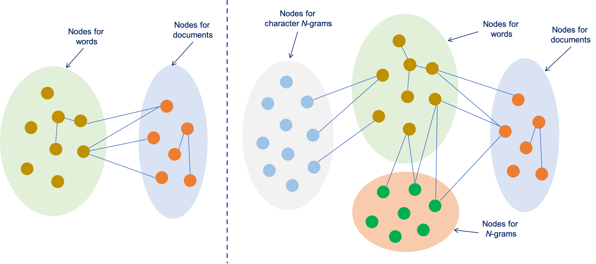
Figure 1: A simple word-document graph (left); and our proposed Word-Character Heterogeneous graph (right). For right figure, the edge types are defined as follows: (1) word-document connection if a document contains a word (i.e., tf-idf); (2) word-word connection based on co-occurrence statistics (i.e., PMI); (3) document-document connection with similarity score (i.e., cosine similarity); (4) word n-grams and words connection if a word is part of n-grams (0/1); (5) word n-grams and document connection if a document contains a n-grams (0/1); and (6) character n-grams and words connection if a character n-grams is part of a word (0/1).

Contributions: In this paper, we propose a new simple yet effective way of constructing graphs from text for GNNs. First, we assume that word ordering plays an important role for semantic understanding which could be captured by higher-order n-gram nodes. Second, we introduce character n-gram nodes as an effective way for mitigating sparsity Bojanowski et al. (2017). Third, we take into account document similarity allowing the model to learn better associations between documents. Figure 1 (right) shows our proposed Word-Character Heterogeneous text graph compared to a standard word-document graph (left). Finally, we propose two variants of GNNs, WCTextGCN and WCTextGAT, that extend GCN and GAT respectively, for modeling our proposed text graph.

2 Methodology

Given a corpus as a list of text documents $\mathcal{C}=\{D_{1},...,D_{n}\}$, our goal is to learn an embedding $\mathbf{h}_{i}$ for each document $D_{i}$ using GNNs. This representation can subsequently be used in different downstream tasks such as text classification and summarization.

2.1 Word-Character Heterogeneous Graph

The Word-Character Heterogeneous graph $G=(V,E)$ consists of the node set $V=V_{d}\cup V_{w}\cup V_{g}\cup V_{c}$, where $V_{d}=\{d_{1},..,d_{n}\}$ corresponds to a set of documents, $V_{w}=\{w_{1},...,w_{m}\}$ denotes a set of unique words, $V_{g}=\{g_{1},...,g_{l}\}$ denotes a set of unique n-gram tokens, and finally $V_{c}=\{c_{1},...,c_{p}\}$ denotes a set of unique character n-grams. The edge types among different nodes vary depending on the types of the connected nodes. In addition, we also add edges between two documents if their cosine similarity is larger than a pre-defined threshold.

2.2 Word and Character N-grams Enhanced Text GNNs

The goal of GNN models is to learn representation for each node. We use $\mathbf{H}^{d}\in R^{n_{d}\times k},\mathbf{H}^{w}\in R^{n_{w}\times k},\mathbf{H}^{g}\in R^{n_{g}\times k},\mathbf{H}^{c}\in R^{n_{c}\times k}$ to denote representations of document nodes, word nodes, word n-grams nodes and character n-grams nodes, where $k$ is the size of the hidden dimension size. $n_{d},n_{w},n_{g},n_{w}$ represent the number of documents, words, word n-grams and character n-grams in the graph respectively. We use $e^{dw}_{ij}$ to denote the edge weight between the $i$th document and $j$th word. Similarly, $e^{cw}_{kj}$ denotes the edge weight between the $k$th character n-gram and $j$th word.

The original GCN and GAT models only consider simple graphs where the graph contains a single type of nodes and edges. Since we now are dealing with our Word-Character Heterogeneous graph, we introduce appropriate modifications.

Word and Character N-grams Enhanced Text GCN (WCTextGCN)

In order to support our new graph type for GCNs, we need a modification for the adjacency matrix $\mathbf{A}$. The updating equation for original GCN is:

$$\mathbf{H}^{(L+1)}=f(\hat{\mathbf{A}}\mathbf{H}^{L}\mathbf{W}_{L})$$

where $W_{L}$ is the free parameter to be learned for layer $L$. We assume $\mathbf{H}$ is simply the concatenation of $\mathbf{H}^{d},\mathbf{H}^{w},\mathbf{H}^{g},\mathbf{H}^{c}$. For WCTextGCN, the adjacency matrix $\mathbf{A}$ is re-defined as:

$$\mathbf{A}=\begin{pmatrix}\mathbf{A}^{dd}_{sim}&\mathbf{A}^{dw}_{tfidf}&\mathbf{A}^{dg}_{tfidf}&-\\ \mathbf{A}^{wd}_{tfidf}&\mathbf{A}^{ww}_{pmi}&\mathbf{A}^{wg}_{0/1}&\mathbf{A}^{wc}_{0/1}\\ \mathbf{A}^{gd}_{tfidf}&\mathbf{A}^{gw}_{0/1}&-&-\\ -&\mathbf{A}^{cw}_{0/1}&-&-\end{pmatrix}$$

where $\mathbf{A}^{dd}_{sim}$ denotes the pair-wise similarity between documents , sub-matrix $\mathbf{A}^{dw}_{tfidf}$ represents the tf-idf score for all edges linking documents to words, $\mathbf{A}^{wg}_{0/1}$ is the boolean sub-matrix representing whether a word n-gram contains a specific word, and so on. The sub-matrix $\mathbf{A}^{dw}_{tfidf}$ is the transpose of sub-matrix $A^{wd}_{tfidf}$.

Word and Character N-grams Enhanced Text GAT WCTextGAT

In GAT, the updates to the node representation is computed by weighting the importance of neighboring nodes. Since our text graph contains four types of nodes, each updating procedure consists of the following four phases (dependency relation among nodes can be seen in Figure 1):

$$\hat{\mathbf{H}}^{d} =\text{GAT}(\mathbf{H}^{d},\mathbf{H}^{w},\mathbf{H}^{g})$$

$$\hat{\mathbf{H}}^{w} =\text{GAT}(\mathbf{H}^{d},\mathbf{H}^{w},\mathbf{H}^{g},\mathbf{H}^{c})$$

$$\hat{\mathbf{H}}^{g} =\text{GAT}(\mathbf{H}^{d},\mathbf{H}^{w})$$

$$\hat{\mathbf{H}}^{c} =\text{GAT}(\mathbf{H}^{w})$$

For example, to update word representation $\hat{\mathbf{H}}^{w}$, we need to aggregate information from document nodes, word nodes, word n-gram nodes and character n-gram nodes, respectively. Assume that we update the embedding for word node $i$ by considering neighboring document nodes only (similar procedure applies to other three types of nodes). The computation is as follows:

$$z_{ij} =\text{Leaky}(a^{T}[\mathbf{W}_{v}\mathbf{h}^{w}_{i};\mathbf{W}_{d}\mathbf{h}^{d}_{j};\mathbf{W}_{e}{e}_{ij}^{wd}])$$

$$\alpha_{ij} =\frac{\exp(z_{ij})}{\sum_{l\in\mathcal{N}_{i}}\exp(z_{il})}$$

$$\hat{\mathbf{h}^{1}_{i}} =\sigma(\sum_{j\in\mathcal{N}_{i}}\alpha_{ij}\mathbf{W}_{d}\mathbf{h}^{d}_{j})$$

where $\mathbf{W}_{v},\mathbf{W}_{d},\mathbf{W}_{e}$ are the trainable weights of the model, that are applied to different types of nodes. $\alpha_{ij}$ is the attention weight between word $i$ and document $j$. $\mathcal{N}_{i}$ denotes the set of neighboring documents for word $i$, and $\sigma(.)$ is the activation function. Multi-head attention Vaswani et al. (2017) is also introduced to capture different aspects of semantic representations for text:

$$\hat{\mathbf{h}^{1}_{i}}=\parallel_{k=1}^{K}\sigma(\sum_{j\in\mathcal{N}_{i}}\alpha^{k}_{ij}\mathbf{W}^{k}_{d}\mathbf{h}_{j})$$

Similarly, we can also compute $\hat{\mathbf{h}^{2}_{i}},\hat{\mathbf{h}^{3}_{i}},\hat{\mathbf{h}^{4}_{i}}$ by considering other types of neighboring nodes. Finally, these representations are concatenated, followed by linear transformation.

Dataset	20NG	R8	R52	Ohsumed	MR
TF-IDF+LR	83.19$\pm$0.00	93.74$\pm$0.00	86.95$\pm$0.00	54.66$\pm$0.00	74.59$\pm$0.00
fastText	79.38$\pm$0.30	96.13$\pm$0.21	92.81$\pm$0.09	57.70$\pm$0.49	75.14$\pm$0.20
CNN-rand	76.83$\pm$0.61	94.02$\pm$0.57	85.37$\pm$0.47	43.87$\pm$1.00	74.98$\pm$0.70
CNN-non-static	82.15$\pm$0.52	95.71$\pm$0.52	87.59$\pm$0.48	58.44$\pm$1.06	77.75$\pm$0.72
LSTM-rand	65.71$\pm$1.52	93.68$\pm$0.82	85.54$\pm$1.13	41.13$\pm$1.17	75.06$\pm$0.44
LSTM-pretrain	75.43$\pm$1.72	96.09$\pm$0.19	90.48$\pm$ 0.86	51.10$\pm$1.50	77.33$\pm$0.89
PTE	76.74$\pm$0.29	96.69$\pm$ 0.13	90.71$\pm$ 0.14	53.58$\pm$ 0.29	70.23$\pm$0.36
BERT	83.41$\pm$0.20	96.98$\pm$ 0.08	92.87$\pm$ 0.01	67.22$\pm$ 0.27	77.02$\pm$0.23
TextGCN	86.34$\pm$0.09	97.07$\pm$ 0.10	93.56$\pm$0.18	68.36$\pm$0.56	76.74$\pm$0.20
WCTextGCN (Ours)	87.21$\pm$0.54	97.49$\pm$0.20	93.88$\pm$0.34	68.52$\pm$0.20	77.85$\pm$ 0.34
TextGAT	85.78$\pm$ 0.10	96.88$\pm$0.24	93.61$\pm$0.12	67.46$\pm$0.32	76.45$\pm$0.38
WCTextGAT (Ours)	87.02$\pm$ 0.32	97.12$\pm$0.42	94.02$\pm$0.45	68.14$\pm$0.18	77.98$\pm$0.10

Table 1: Predictive test accuracy on five text classification benchmark datasets. We run models 10 times and report mean$\pm$standard deviation.

3 Experiments and Results

We conduct experiments on two NLP tasks, i.e., text classification and extractive summarization. The latter one can be also viewed as a classification problem for each sentence level (i.e., to be included in the summary or not).

3.1 Text Classification

Data

We select five widely used benchmark datasets including 20-Newsgroups, Ohsumed, R52, R8 and MR. The statistics and the descriptions for these datasets can be found in Yao et al. (2019).

Baselines

We compare our models to multiple existing state-of-the-art text classification methods including TF-IDF+LR, fastText Joulin et al. (2016), CNN Le and Mikolov (2014), LSTM Liu et al. (2016), PTE Tang et al. (2015), BERT Devlin et al. (2018), TextGCN Yao et al. (2019) and TextGAT.

R8	3	4	5	6
3	97.1	97.5	97.5	97.4
4		96.9	97.1	97.5
5			97.1	97.4
6				97.4

R52	3	4	5	6
3	93.5	93.8	93.8	93.7
4		93.4	93.6	93.8
5			93.6	93.7
6				93.8

MR	3	4	5	6
3	76.8	78.2	78.3	78.3
4		77.2	78.2	78.3
5			78.1	78.1
6				77.9

Table 2: The effect on performance by using character n-grams of $n$ in {3,..,6}.

Experimental Settings

We randomly select 10% of the training set for the validation. For the WCTextGCN model, we set the hidden size to $200$. For the TextGAT and WCTextGAT models, we use $8$ attention heads with each containing $16$ hidden units, and set edge feature dimension to $32$. The learning rate is $0.002$ and dropout rate $0.5$. We train all models for $200$ epochs using Adam optimizer Kingma and Ba (2014) and early stopping with patience $20$. For all the GNNs models, we use two hidden layers and $1$-of-$K$ encoding for initialization.

Results

Table 1 shows the text classification results. We observe that the incorporation of word n-grams, character n-grams and document similarity are helpful and consistently improve predictive performance over other models. i.e., the WCTextGCN model improves accuracy on 20NG over 0.8% compared to the TextGCN model. The improvements in MR and R8 datasets are more substantial than others, 0.5% and 1.1%, respectively. This is because character n-grams help more when text is short, which is consistent with our hypothesis that character n-grams are helpful for mitigating sparsity problems.

Varying the size of n-grams

For character n-grams, we set n-grams ranging from $3$ to $6$ characters, and record the performance in different combinations of n-grams, i.e., $3$-grams to $4$-grams, $3$-grams to $5$-grams and so on. The results are shown in Table 2 with best scores in bold. We observe that the best results are often obtained when we vary the range of $n$ from $3$ to $4$. Further increase of $n$ provides limited effects in model performance. In terms of word $n$-grams, we observe similar results.

3.2 Extractive Text Summarization

Extractive single-document summarization is formulated as a binary classification for each sentence with the aim to predict whether a sentence should be included in the summary or not. We follow the same setting as the HeterogeneousSumGraph (HSG) proposed by Wang et al. (2020) except that we use our new Word-Character Heterogeneous graph representation denoted as HSG-Ours.

Data

We select two widely used benchmark newes articles datasets, CNN/DailyMail (Hermann et al., 2015) and NYT50 Durrett et al. (2016). The first contains 287,227/13,368/11,490 examples for training, validation and test. The second contains 110,540 articles with their summaries and is split into 100,834 and 9,706 for training and test. Following Durrett et al. (2016), we use the last 4,000 documents from the training set for validation and 3,452 test examples.

Baselines and Experimental Settings

We evaluate our models on single document summarization by comparing to three different baselines Wang et al. (2020), Ext-BILSTM, Ext-Transformer and HSG. For all experiments, we simply follow the same settings as in Wang et al. (2020) and evaluate performance using ROUGE Lin and Hovy (2003).

Results

Tables 3 and 4 show the ROUGE scores on the two datasets. HGS-Ours with our new text graph performs consistently better than competing ones. In particular, for NYT50 data, the R-1 and R-2 metrics improve more than $0.5$ compared to the HSG model. We observe similar performance differences for R-L on CNN/DailyMail data. This highlights the efficacy of our new text graph in learning better word and sentence representations, especially for the words that appear only few times but play an important role in summarization.

Model	R-1	R-2	R-L
Ext-BiLSTM	46.32	25.84	42.16
Ext-Transformer	45.07	24.72	40.85
HSG	46.89	26.26	42.58
HSG-Ours	46.96	26.20	43.43

Table 3: Performance (ROUGE) of different models on CNN/DailyMail.

Model	R-1	R-2	R-L
Ext-BiLSTM	41.59	19.03	38.04
Ext-Transformer	41.33	18.83	37.65
HSG	42.31	19.51	38.74
HSG-Ours	42.85	20.03	38.90

Table 4: Performance (ROUGE) of different models on NYT50.

4 Conclusion

In this paper, we proposed a new text graph representation by incorporating word and character level information. GNN models trained using our text graph provide superior performance in text classification and single-document summarization compared to previous work. In the future, we plan to extend our proposed method to other tasks such as opinion extraction Mensah et al. (2021), misinformation detection Chandra et al. (2020); Mu and Aletras (2020); Mu et al. (2022), voting intention forecasting Tsakalidis et al. (2018) and socioeconomic attribute analysis Aletras and Chamberlain (2018). We finally plan to extend our GNN models by weighting the contribution of neighboring nodes Zhang et al. (2022).

References

- Aletras and Chamberlain (2018) Nikolaos Aletras and Benjamin Paul Chamberlain. 2018. Predicting twitter user socioeconomic attributes with network and language information. In Proceedings of the 29th on Hypertext and Social Media, pages 20–24.
- An et al. (2021) Chenxin An, Ming Zhong, Yiran Chen, Danqing Wang, Xipeng Qiu, and Xuanjing Huang. 2021. Enhancing scientific papers summarization with citation graph. In Proceedings of the AAAI Conference on Artificial Intelligence, volume 35, pages 12498–12506.
- Bojanowski et al. (2017) Piotr Bojanowski, Edouard Grave, Armand Joulin, and Tomas Mikolov. 2017. Enriching word vectors with subword information. Transactions of the Association for Computational Linguistics, 5:135–146.
- Chandra et al. (2020) Shantanu Chandra, Pushkar Mishra, Helen Yannakoudakis, Madhav Nimishakavi, Marzieh Saeidi, and Ekaterina Shutova. 2020. Graph-based modeling of online communities for fake news detection. arXiv preprint arXiv:2008.06274.
- Devlin et al. (2018) Jacob Devlin, Ming-Wei Chang, Kenton Lee, and Kristina Toutanova. 2018. Bert: Pre-training of deep bidirectional transformers for language understanding. arXiv preprint arXiv:1810.04805.
- Durrett et al. (2016) Greg Durrett, Taylor Berg-Kirkpatrick, and Dan Klein. 2016. Learning-based single-document summarization with compression and anaphoricity constraints. In Proceedings of the 54th Annual Meeting of the Association for Computational Linguistics (Volume 1: Long Papers), pages 1998–2008.
- Hermann et al. (2015) Karl Moritz Hermann, Tomáš Kočiskỳ, Edward Grefenstette, Lasse Espeholt, Will Kay, Mustafa Suleyman, and Phil Blunsom. 2015. Teaching machines to read and comprehend. arXiv preprint arXiv:1506.03340.
- Joulin et al. (2016) Armand Joulin, Edouard Grave, Piotr Bojanowski, and Tomas Mikolov. 2016. Bag of tricks for efficient text classification. arXiv preprint arXiv:1607.01759.
- Kingma and Ba (2014) Diederik P Kingma and Jimmy Ba. 2014. Adam: A method for stochastic optimization. arXiv preprint arXiv:1412.6980.
- Kipf and Welling (2016) Thomas N Kipf and Max Welling. 2016. Semi-supervised classification with graph convolutional networks. arXiv preprint arXiv:1609.02907.
- Le and Mikolov (2014) Quoc Le and Tomas Mikolov. 2014. Distributed representations of sentences and documents. In International conference on machine learning, pages 1188–1196. PMLR.
- Li et al. (2020) Chen Li, Xutan Peng, Hao Peng, Jianxin Li, Lihong Wang, and S Yu Philip. 2020. Textsgcn: Document-level graph topology refinement for text classification.
- Liang et al. (2022) Bin Liang, Hang Su, Lin Gui, Erik Cambria, and Ruifeng Xu. 2022. Aspect-based sentiment analysis via affective knowledge enhanced graph convolutional networks. Knowledge-Based Systems, 235:107643.
- Lin and Hovy (2003) Chin-Yew Lin and Eduard Hovy. 2003. Automatic evaluation of summaries using n-gram co-occurrence statistics. In Proceedings of the 2003 human language technology conference of the North American chapter of the association for computational linguistics, pages 150–157.
- Liu et al. (2016) Pengfei Liu, Xipeng Qiu, and Xuanjing Huang. 2016. Recurrent neural network for text classification with multi-task learning. arXiv preprint arXiv:1605.05101.
- Mensah et al. (2021) Samuel Mensah, Kai Sun, and Nikolaos Aletras. 2021. An empirical study on leveraging position embeddings for target-oriented opinion words extraction. In Proceedings of the 2021 Conference on Empirical Methods in Natural Language Processing, pages 9174–9179, Online and Punta Cana, Dominican Republic. Association for Computational Linguistics.
- Minaee et al. (2021) Shervin Minaee, Nal Kalchbrenner, Erik Cambria, Narjes Nikzad, Meysam Chenaghlu, and Jianfeng Gao. 2021. Deep learning–based text classification: A comprehensive review. ACM Computing Surveys (CSUR), 54(3):1–40.
- Mu and Aletras (2020) Yida Mu and Nikolaos Aletras. 2020. Identifying twitter users who repost unreliable news sources with linguistic information. PeerJ Computer Science, 6:e325.
- Mu et al. (2022) Yida Mu, Pu Niu, and Nikolaos Aletras. 2022. Identifying and characterizing active citizens who refute misinformation in social media. In 14th ACM Web Science Conference 2022, WebSci ’22, page 401–410, New York, NY, USA. Association for Computing Machinery.
- Ragesh et al. (2021) Rahul Ragesh, Sundararajan Sellamanickam, Arun Iyer, Ramakrishna Bairi, and Vijay Lingam. 2021. Hetegcn: Heterogeneous graph convolutional networks for text classification. In Proceedings of the 14th ACM International Conference on Web Search and Data Mining, pages 860–868.
- Scarselli et al. (2008) Franco Scarselli, Marco Gori, Ah Chung Tsoi, Markus Hagenbuchner, and Gabriele Monfardini. 2008. The graph neural network model. IEEE transactions on neural networks, 20(1):61–80.
- Tang et al. (2015) Jian Tang, Meng Qu, and Qiaozhu Mei. 2015. Pte: Predictive text embedding through large-scale heterogeneous text networks. In Proceedings of the 21th ACM SIGKDD international conference on knowledge discovery and data mining, pages 1165–1174.
- Tsakalidis et al. (2018) Adam Tsakalidis, Nikolaos Aletras, Alexandra I Cristea, and Maria Liakata. 2018. Nowcasting the stance of social media users in a sudden vote: The case of the greek referendum. In Proceedings of the 27th ACM International Conference on Information and Knowledge Management, pages 367–376.
- Vaswani et al. (2017) Ashish Vaswani, Noam Shazeer, Niki Parmar, Jakob Uszkoreit, Llion Jones, Aidan N Gomez, Lukasz Kaiser, and Illia Polosukhin. 2017. Attention is all you need. arXiv preprint arXiv:1706.03762.
- Veličković et al. (2017) Petar Veličković, Guillem Cucurull, Arantxa Casanova, Adriana Romero, Pietro Lio, and Yoshua Bengio. 2017. Graph attention networks. arXiv preprint arXiv:1710.10903.
- Wang et al. (2020) Danqing Wang, Pengfei Liu, Yining Zheng, Xipeng Qiu, and Xuanjing Huang. 2020. Heterogeneous graph neural networks for extractive document summarization. arXiv preprint arXiv:2004.12393.
- Yao et al. (2021) Huaxiu Yao, Yingxin Wu, Maruan Al-Shedivat, and Eric P Xing. 2021. Knowledge-aware meta-learning for low-resource text classification. arXiv preprint arXiv:2109.04707.
- Yao et al. (2019) Liang Yao, Chengsheng Mao, and Yuan Luo. 2019. Graph convolutional networks for text classification. In Proceedings of the AAAI Conference on Artificial Intelligence, volume 33, pages 7370–7377.
- Zhang et al. (2022) Li Zhang, Heda Song, Nikolaos Aletras, and Haiping Lu. 2022. Node-feature convolution for graph convolutional networks. Pattern Recognition, 128:108661.