Abstract The goodness of the long-term prediction in the state-space model was evaluated using the squared long-term prediction error. In order to estimate the model parameters suitable for long-term prediction, we devised a modified log-likelihood corresponding to the long-term prediction error variance. Trend models and seasonally adjusted models with and without AR component are examined as examples.

1 Introduction: State-Space Modeling of Time Series

1.1 State-Space Model and State Estimation

Consider the state-space model of a univaraite time series $y_{n}$;

$$x_{n} = F_{n}x_{n-1}+G_{n}v_{n},\hskip 31.2982pt\mbox{(system model)}$$ (1)

$$y_{n} = H_{n}x_{n}+w_{n},\hskip 50.64586pt\mbox{(observation model)}$$ (2)

where $x_{n}$ is a $k$-dimensional state vector, $v_{n}$ is an $m$-dimensional system noise that follows a white noise with mean vector zero and variance-covariance matrix $Q_{n}$, and $w_{n}$ is the observation noise that follows a 1-dimensional Gaussian white noise with mean zero and the variance $R_{n}$. $F_{n}$, $G_{n}$, and $H_{n}$ are $k\times k$, $k\times m$, $k\times 1$ and $1\times k$ matrices, respectively. The initial state vector $x_{0}$ is assumed to follow the Gaussian distribution, $N(0,V_{0|0})$. Many linear models used in time series analysis such as the AR model, ARMA model and various nonstationary models such as the trend model and the seasonal adjustment model are expressible in terms of the state-space models (Anderson and Moore (1979), Kitagawa (2020)).

In this paper, we shall consider the problem of estimating the state $x_{n}$ at time $n$ based on the set of observations $Y_{j}=\{y_{1},\cdots,y_{j}\}$. For $j<n$, $j=n$, and $j>n$, the state estimation problem is referred to as the prediction, filter and smoothing, respectively. This state estimation problem is important in state-space modeling since many tasks such as one-step-ahead and multi-step-ahead prediction, interpolation, and likelihood computation for the time series can be systematically solved through the estimated state.

A generic approach to these state estimation problems is to obtain the conditional distribution $p(x_{n}|Y_{j})$ of the state $x_{n}$ given the observations $Y_{j}$. Then, since the state-space model defined by (1) and (2) is a linear model, and moreover the noises $v_{n}$ and $w_{n}$, and the initial state $x_{0}$ follow normal distributions, all these conditional distributions become normal distributions. Therefore, to solve the problem of state estimation of the state-space model, it is sufficient to obtain the mean vectors $x_{n|j}$ and the variance-covariance matrices $V_{n|j}$ of the conditional distributions.

For the linear state-space model, Kalman filter provides a computationally efficient recursive computational algorithm for state estimation (Kalman (1960), Anderson and Moore (1976)).

One-step-ahead prediction

$$x_{n|n-1} = F_{n}x_{n-1|n-1}$$

$$V_{n|n-1} = F_{n}V_{n-1|n-1}F_{n}^{T}+G_{n}Q_{n}G_{n}^{T}.$$ (3)

Filter

$$K_{n} = V_{n|n-1}H_{n}^{T}(H_{n}V_{n*n-1}H_{n}^{T}+R_{n})^{-1}$$

$$x_{n|n} = x_{n|n-1}+K_{n}(y_{n}-H_{n}x_{n|n-1})$$ (4)

$$V_{n|n} = (I-K_{n}H_{n})V_{n|n-1}.$$

1.2 Likelihood Computation and Parameter Estimation for Time Series Models

Assume that the state-space representation for a time series model specified by a parameter $\theta$ is given. When the time series $y_{1},\cdots,y_{N}$ of length $N$ is given, the $N$ dimensional joint density function of $y_{1},\cdots,y_{N}$ specified by this time series model is denoted by $f_{N}(y_{1},\cdots,y_{N}|\theta)$. Then, the likelihood of this model is defined by $L(\theta)=f_{N}(y_{1},\cdots,y_{N}|\theta)$. Using the conditional distribution of $y_{n}$ given the previous observations, the likelihood of the time series model can be expressed as a product of one-dimentional conditional density functions:

$$L(\theta)=\prod_{n=1}^{N}g_{n}(y_{n}|y_{1},\cdots,y_{n-1},\theta)=\prod_{n=1}^{N}g_{n}(y_{n}|Y_{n-1},\theta).$$ (5)

Here, if we define $Y_{0}=\emptyset$ (empty set), then $g_{1}(y_{1}|Y_{0},\theta)\equiv f_{1}(y_{1}|\theta)$. By taking the logarithm of $L(\theta)$, the log-likelihood of the model is obtained as

$$\ell(\theta)=\log L(\theta)=\sum_{n=1}^{N}\log g_{n}(y_{n}|Y_{n-1},\theta).$$ (6)

Since $g_{n}(y_{n}|Y_{n-1},\theta)$ is the conditional distribution of $y_{n}$ given the observation $Y_{n-1}$ and it is, in fact, a normal distribution with mean $y_{n|n-1}$ and variance $d_{n|n-1}$, it can be expressed as (Kitagawa and Gersch (1996))

$$g_{n}(y_{n}|Y_{n-1},\theta)=\left(2\pi d_{n|n-1}\right)^{-\frac{1}{2}}\exp\left\{-\frac{(y_{n}-y_{n|n-1})^{2}}{2d_{n|n-1}}\right\}.$$ (7)

Here, from the observation model, (2), $y_{n|n-1}$ and $d_{n|n-1}$ are obtained by

$$y_{n|n-1} = H_{n}x_{n|n-1}$$ (8)

$$d_{n|n-1} = H_{n}V_{n|n-1}H_{n}^{T}+R_{n}.$$ (9)

Therefore, by substituting this density function into (6), the log-likelihood of this state-space model is obtained as

$$\ell(\theta)=-\frac{1}{2}\biggl{\{}N\log 2\pi+\sum_{n=1}^{N}\log d_{n|n-1}+\sum_{n=1}^{N}\frac{(y_{n}-y_{n|n-1})^{2}}{d_{n|n-1}}\biggr{\}}.$$ (10)

The maximum likelihood estiamtes of the parameters of the state-space model can be obtained by maximizing this log-likelihood function numerically. However, for univariate time series, we can assume that $R=1$ (Kitagawa (2020)). Actually, if $\tilde{V}_{n|n}$, $\tilde{V}_{n|n-1}$, $\tilde{Q}_{n}$, and $\tilde{R}$ are defined by

$$V_{n|n-1}=\sigma^{2}\tilde{V}_{n|n-1},\quad V_{n|n}=\sigma^{2}\tilde{V}_{n|n},\quad Q_{n}=\sigma^{2}\tilde{Q}_{n},\quad\tilde{R}=1,$$ (11)

then it can be seen that the obtained Kalman gain $\tilde{K}_{n}$ is identical to $K_{n}$. Therefore, in the filtering step, we may use $\tilde{V}_{n|n}$ and $\tilde{V}_{n|n-1}$ instead of $V_{n|n}$ and $V_{n|n-1}$. Furthermore, it can be seen that the vectors $x_{n|n-1}$ and $x_{n|n}$ of the state do not change under these modifications. In summary, if $R_{n}$ is time-invariant and $R=\sigma^{2}$ is an unknown parameter, we may apply the Kalman filter by setting $R=1$. Since we then have $d_{n|n-1}=\sigma^{2}\tilde{d}_{n|n-1}$ from (10), this yields

$$\ell(\theta)=-\frac{1}{2}\left\{N\log 2\pi\sigma^{2}+\sum_{n=1}^{N}\log\tilde{d}_{n|n-1}+\frac{1}{\sigma^{2}}\sum_{n=1}^{N}\frac{(y_{n}-y_{n|n-1})^{2}}{\tilde{d}_{n|n-1}}\right\}.$$

(12)

From the likelihood equation

$$\frac{\partial\ell(\theta)}{\partial\sigma^{2}}=-\frac{1}{2}\left\{\frac{N}{\sigma^{2}}-\frac{1}{(\sigma^{2})^{2}}\sum_{n=1}^{N}\frac{(y_{n}-y_{n|n-1})^{2}}{\tilde{d}_{n|n-1}}\right\}=0,$$ (13)

the maximum likelihood estimate of $\sigma^{2}$ is obtained by

$$\hat{\sigma}^{2}=\frac{1}{N}\sum_{n=1}^{N}\frac{(y_{n}-y_{n|n-1})^{2}}{\tilde{d}_{n|n-1}}.$$ (14)

Furthermore, denoting the parameters in $\theta$ except for the variance $\sigma^{2}$ by $\theta^{\ast}$, and substituting (14) into (12), we have an expression for the log-likelihood

$$\ell(\theta^{\ast})=-\frac{1}{2}\left(N\log 2\pi\hat{\sigma}^{2}+\sum_{n=1}^{N}\log\tilde{d}_{n|n-1}+N\right).$$ (15)

1.3 Parameter Estimation and Criterion for Increasing Horizon Prediction of the State

For the state-space model, by repeating the one-step-ahead prediction step, we can perform increasing horizon prediction, that is, we can obtain $x_{n+j|n}$ and $V_{n+j|n}$ for $j=1,2,\cdots p$.

The increasing horizon prediction

For $j=1,\cdots,p$, repeat

$$x_{n+j|n} = F_{n+j}x_{n+j-1|n}$$

$$V_{n+j|n} = F_{n+j}V_{n+j-1|n}F_{n+j}^{T}\>+\>G_{n+j}Q_{n+j}G_{n+j}^{T}.$$ (16)

The long-term prediction is considered by many authors such as Judd and Small (2000), Sorjamaa et. al. (2007) and Xiong et. al. (2013). In this paper, we evaluate the goodness of the long-term prediction by the difference between the predictied value and the observed value

$$\hat{\sigma}^{2}_{p}=\frac{1}{N-p}\sum_{n=1}^{N-p}\varepsilon_{n+p|n}^{2},$$ (17)

where $p$-step-ahead prediction error is defined by $\varepsilon_{n+p|n}=y_{n+p}-y_{n+p|n}$ and $y_{n+p|n}$ is defined by $y_{n+p|n}=Hx_{n+p|n}$. We can also consider a modified log-likelihood for the long-term prediction defined by

$$\ell_{p}(\theta)=-\frac{1}{N-p}\left\{(N-p)(\log 2\pi\hat{\sigma}^{2}_{p}+1)+\sum_{n=1}^{N-p}\log d_{n+p|n}\right\}$$ (18)

where $d_{n+k|n}$ is obtained by $d_{n+p|n}=H_{n+p}V_{n+p|n}H_{n+p}^{T}+R_{n+p}$. Note that, different from the case of one-step-ahead prediction errors, the long-term prediction errors, $\varepsilon_{p+1|1},\ldots,\varepsilon_{N|N-p}$ are not independent.

Given the predetermined prediction horizon $p$, the optimal value of the parameter vector $\theta$ for $p$-step-ahead prediction is obtained by maximizing this modified log-likelihood.

2 Examples

2.1 Trend models

2.1.1 The secon order trend model

We consider the second order trend model

$$y_{n}=T_{n}+w_{n},$$ (19)

where $T_{n}$ is the trend component that follows the second order trend component model $T_{n}=2T_{n-1}-T_{n-2}+v_{n}$ and $w_{n}$ and $v_{n}$ are Gaussian white noise $w_{n}\sim N(0,\sigma^{2})$ and $v_{n}\sim N(0,\tau^{2})$, respectively. Note that this trend model can be expressed by a state-space model by

$$x_{n}=\left[\begin{array}[]{l}T_{n}\\ T_{n-1}\end{array}\right],\quad F=\left[\begin{array}[]{cc}2&-1\\ 1&0\end{array}\right],\quad G=\left[\begin{array}[]{c}1\\ 0\end{array}\right],\quad H=\left[\begin{array}[]{cc}1&0\end{array}\right].$$ (27)

Figure 1 shows the trend estimates of the maxtemp data (daily maximum temperature data in Tokyo, N=486). Smoothed estimate (red) and $\pm$2SD interval are shown. Top left plot shows the estimates obtained by the ordinary maximum likelihood method, i.e., by $p=1$. On the other hand, three other plots show the results obtained by modified log-likelihood criteria asumming $p=1,5$ and 20, respectively. It can be seen that the trend estimate by $p=1$ is considerably variable compared with other three estimates, and other three estimates obtained with $p>1$ resemble each other.

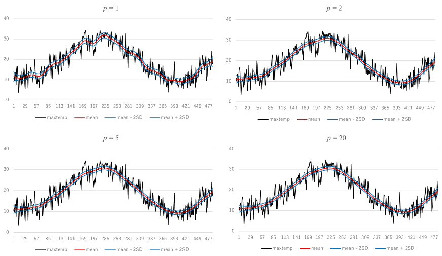
Figure 1: The estimated trend of the maximum temperature data obtained by the second order trend models estimated by the $p$-step-ahead prediction criterion, $p$=1, 2, 5 and 20. Each plot shows the data (black), the mean (red) , mean$\pm$ 2SD (blue) of the estimated trend components.

Table 1 shows the increasing horizon prediction error variances $\hat{\sigma}_{j}^{2}$, $j=1,\ldots,20$, for various parameter estimation criteria $\ell_{p}(\theta)$, $p$=1,(1),6,(2),20. The results for $p=1$ shown in the second column are the increasing horaizon prediction error variances of the model obtained by the maximum-likelihood method. In general, $(j,p)$-element of the table shows the $j$-step-ahead prediction error variance of the model whose parameter was obtained by maximizing the modified log-likelihood for $p$-step-ahead prediction criterion (18). Naturally, the one-step-ahead prediction error variance $\hat{\sigma}_{1}^{2}$ attains the smallest value 9.89 with $p=1$, but the long-term prediction error variances, i.e., for $j>1$, $\hat{\sigma}_{j}^{2}$ becomes the largest among $p=1,\ldots,20$. The table also shows that the $j$-step-ahead prediction error variance is the smallest at the criterion $p$. For $p>1$, the increase of the long-term prediction error varaince is not so significant and $\hat{\sigma}_{j}^{2}$ takes similar values for different $p$. The last row of the table shows the average of the long-term prediction error varainces, $\hat{\sigma}_{j}^{2}$, over $j=1,\ldots,20$ for each $p$.

Table 1: Long-term prediction error variances of trend models with $m_{1}=2$ for various $p$.

						$p$
$j$	1	2	3	4	5	6	8	10	12	14	16	18	20
1	9.89	10.02	10.05	10.07	10.07	10.08	10.13	10.15	10.16	10.17	10.20	10.22	10.20
2	10.92	10.52	10.52	10.53	10.53	10.53	10.56	10.58	10.58	10.59	10.62	10.64	10.62
3	11.93	11.18	11.16	11.16	11.16	11.16	11.18	11.19	11.20	11.20	11.22	11.24	11.22
4	12.78	11.60	11.57	11.55	11.55	11.55	11.55	11.55	11.56	11.56	11.58	11.59	11.58
5	13.62	12.07	12.02	12.00	12.00	11.99	11.97	11.98	11.98	11.98	12.00	12.01	12.00
6	14.46	12.58	12.51	12.48	12.48	12.46	12.43	12.43	12.43	12.43	12.44	12.45	12.44
7	15.82	13.60	13.51	13.47	13.47	13.45	13.41	13.40	13.40	13.40	13.41	13.42	13.41
8	17.32	14.52	14.41	14.35	14.35	14.33	14.26	14.25	14.24	14.24	14.24	14.24	14.24
9	18.58	15.22	15.09	15.02	15.02	14.98	14.90	14.88	14.88	14.87	14.86	14.87	14.86
10	19.23	15.39	15.23	15.15	15.15	15.11	15.02	15.00	14.99	14.99	14.98	14.98	14.98
11	20.40	15.88	15.70	15.62	15.61	15.57	15.46	15.43	15.42	15.41	15.40	15.40	15.40
12	20.88	15.99	15.80	15.71	15.71	15.66	15.55	15.53	15.52	15.51	15.50	15.51	15.50
13	22.18	16.64	16.43	16.33	16.33	16.27	16.15	16.11	16.11	16.10	16.08	16.08	16.08
14	23.56	17.28	17.04	16.93	16.93	16.87	16.73	16.69	16.68	16.67	16.65	16.65	16.66
15	25.22	18.00	17.72	17.59	17.59	17.52	17.35	17.31	17.30	17.28	17.26	17.26	17.26
16	27.35	18.79	18.46	18.30	18.30	18.22	18.01	17.95	17.94	17.92	17.89	17.87	17.89
17	30.28	20.38	20.01	19.82	19.82	19.72	19.48	19.41	19.40	19.37	19.33	19.31	19.33
18	32.65	21.51	21.10	20.89	20.89	20.78	20.52	20.43	20.42	20.39	20.35	20.32	20.35
19	33.84	21.88	21.46	21.25	21.25	21.14	20.88	20.80	20.79	20.77	20.72	20.71	20.73
20	35.03	22.49	22.07	21.87	21.86	21.76	21.51	21.44	21.43	21.41	21.38	21.37	21.38
	21.51	16.09	15.89	15.80	15.80	15.75	15.64	15.61	15.60	15.59	15.58	15.59	15.58

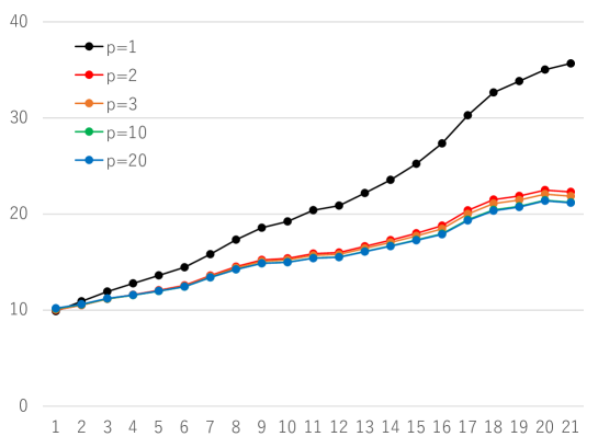
Figure 2: The long-term prediction error variances of maximum temperature data by the second order trend model. Prediction lead time $p$=1, 2, 3, 10 and 20.

Figure 2 shows the increase of the long-term prediction error variance $\hat{\sigma}_{j}^{2}$, $j=1,\ldots,20$ for $p=$1, 2, 3, 10 and 20. We can see that the long-term prediction error variances obtained by $p=1$ are significantly larger than other cases, and there is almost no difference in the prediction error variances among $p=2$, 3, 10 and 20.

From the table and the figure, it can be concluded, at least for this data set, that the model with the maximum likelihood estimates of the patameter has the minimum one-step-ahead prediction error variance but has the largest long-term prediction error varainces. For this second order trend model $p=2,\ldots,20$ yield a similar increasing horaizon prediction performances.

2.1.2 The first order trend model

Figure 3 and Table 2 show similar results for the first order trend model,

$$T_{n}=T_{n-1}+v_{n},\qquad v_{n}\sim N(0,\tau^{2}).$$ (28)

As can be seen in the figure, in this case, different from the case of $k=2$, the estimated trends are wiggly and the change of the estimated trends by the selection of the prediction horaizon $p$ are not so significant.

From the table, it is seen that the one-step-ahead prediction error variances are smaller than those of the second order trend model for entire $p$. Also, the increase of the prediction error variance with the increase of the prediction horaizon is not so large as the second order trend model. Further, it is interesting that the inreasing horaison predictive ability is almost the same for all criterion parameter $p$. The table also shows that the increasing horizon prediction performance is quite similar for various choise of $p$. Note that for the first order trend model, $j$-step-ahead prediction error variance is obtained by

$$V_{n+j|n}=V_{n+j-1|n}+\tau^{2}.$$ (29)

Compared with the results of the second order trend model, at least for the presend data, inspite of the wiggly trend estimate, the first order trend model has slightly better prediction ability than the second order trend model.

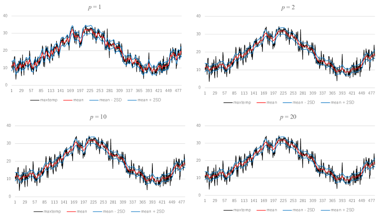
Figure 3: The estimated trend of maximum temperature data by the first order trend model. Prediction lead time $p$=0, 1, 5 and 20. Each plot shows the data (black), the mean (red) , mean$\pm 2$SD (blue) of the estimated trend components.

Table 2: Long-term prediction error variances of trend models with $m_{1}=1$ for various $p$.

	1	2	3	4	5	6	8	10	12	14	16	18	20
1	8.86	9.06	9.12	9.17	9.17	9.12	9.09	9.06	8.99	8.90	8.91	9.07	9.03
2	10.34	9.95	9.95	9.95	9.95	9.95	9.94	9.95	9.97	10.08	10.07	9.95	9.95
3	11.22	10.68	10.67	10.66	10.66	10.67	10.67	10.68	10.73	10.89	10.87	10.68	10.70
4	12.01	11.31	11.28	11.27	11.27	11.28	11.30	11.31	11.39	11.59	11.57	11.30	11.34
5	12.59	11.82	11.79	11.78	11.78	11.79	11.80	11.82	11.90	12.12	12.10	11.81	11.85
6	12.88	12.24	12.22	12.22	12.22	12.22	12.22	12.24	12.29	12.48	12.45	12.23	12.25
7	13.18	12.67	12.67	12.68	12.68	12.67	12.67	12.67	12.71	12.85	12.83	12.67	12.68
8	13.88	13.30	13.30	13.30	13.30	13.30	13.30	13.30	13.35	13.51	13.49	13.30	13.32
9	14.39	13.79	13.78	13.79	13.79	13.78	13.78	13.79	13.83	14.00	13.98	13.78	13.80
10	14.70	14.14	14.14	14.16	14.16	14.14	14.14	14.14	14.17	14.32	14.30	14.14	14.15
11	15.30	14.67	14.67	14.68	14.68	14.67	14.66	14.67	14.70	14.87	14.85	14.66	14.67
12	15.30	14.92	14.96	14.99	14.99	14.95	14.94	14.92	14.91	14.99	14.98	14.93	14.91
13	15.65	15.42	15.47	15.51	15.51	15.46	15.44	15.42	15.38	15.41	15.40	15.43	15.40
14	15.87	15.84	15.90	15.96	15.96	15.90	15.87	15.84	15.77	15.74	15.74	15.85	15.81
15	16.39	16.48	16.55	16.61	16.61	16.55	16.51	16.48	16.40	16.34	16.34	16.49	16.44
16	17.52	17.48	17.53	17.58	17.58	17.53	17.50	17.48	17.43	17.42	17.42	17.49	17.46
17	18.81	18.52	18.55	18.58	18.57	18.54	18.53	18.52	18.52	18.59	18.58	18.52	18.51
18	19.99	19.43	19.43	19.45	19.45	19.43	19.43	19.43	19.47	19.62	19.61	19.43	19.44
19	20.74	20.11	20.11	20.13	20.13	20.11	20.11	20.11	20.15	20.32	20.30	20.11	20.12
20	20.97	20.48	20.51	20.54	20.54	20.51	20.49	20.48	20.49	20.62	20.60	20.49	20.48
21	21.46	21.00	21.03	21.07	21.07	21.03	21.02	21.00	21.00	21.11	21.10	21.01	21.00
	15.34	14.92	14.93	14.96	14.96	14.93	14.92	14.92	14.93	15.04	15.02	14.92	14.92

2.2 Seasonal adjustment model

2.2.1 Standard seassonal adjustment model

We consider here the seasonal adjustment model for the blsallhood data (Buleau of Labor Statistics, all food data, N=156, Kitagawa (2020)),

$$y_{n}=T_{n}+S_{n}+w_{n},$$ (30)

where $T_{n}$ and $S_{n}$ are the trend and the seasonal components that follow

$$T_{n} = 2T_{n-1}-T{n-2}+u_{n}$$

$$S_{n} = -(S_{n-1}+\cdots+S_{n-11})+v_{n}.$$ (31)

Figure 4 shows the decomposition of the data into trend, seasonal component and the observation noise. The left plot shows the case of the maximum likelihood estimate, i.e., obtained by $p=1$. The right plot is the case of $p=2$. It can be seen that compared with the standard results obtained by the maximum likelihood estimates, the estimated trend by $p$=2 is smoother. Similarly, Figure 5 show the cases of $p$=6 and 12. In these cases, the trend become further smoother. No significan difference is seen between the results of $p$=6 and 12. The seasonal components are almost the same for all cases, and the observation noise components of $p=6$ and $p=12$ are almost identical.

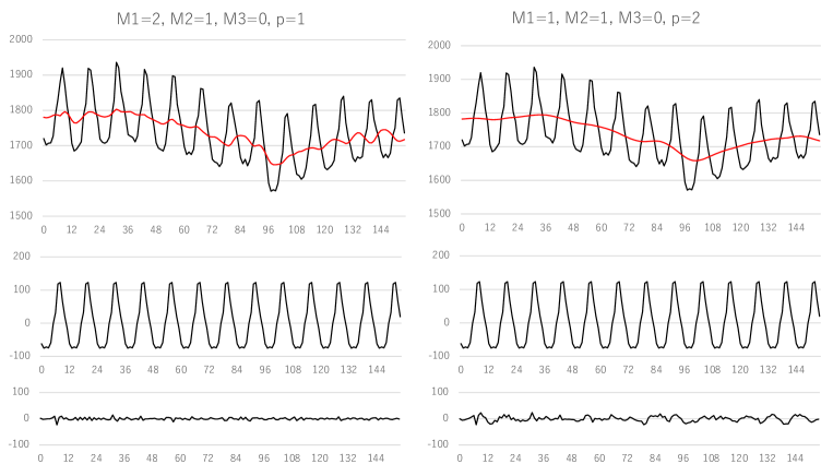
Figure 4: The seasonal adjustment of blsallfood data with $m_{1}=2$ and $m_{2}=1$. Prediction lead time $p$=0 and 1. Top plot shows the data (black) and the mean of the trend(red), the second plot the seasonal component and the bottom plot shows the noise component.

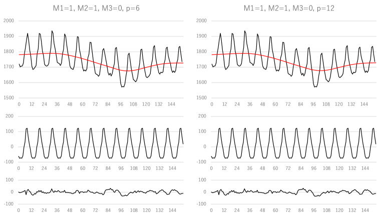
Figure 5: The seasonal adjustment of blsallfood data with $m_{1}=2$ and $m_{2}=1$. Prediction lead time $p$=6 and 12. Top plot shows the data (black) and the mean of the trend(red), the second plot the seasonal component and the bottom plot shows the noise component.

Table 3 shows the increasing horaizon prediction error variances of the seasonal adjustment model obtained with $p=1,\ldots,24$. In this case, the one-step-ahead prediction error variance $\hat{\sigma}^{2}_{1}$ of the maximum likelihood estiamte, obtained by $p=1$, is 133 and is significantly smaller than other $p$. This indicates that the maximum likelihood estimate has siginificantly better one-step-ahead prediction performance than the other $p$. However, the increase of the variance for increasing prediction horaizon $j$ is significant and takes the largest long-term prediction variances for $j\geq 3$ among all prediction horizon $p=1,\ldots,24$. For $p\geq 6$ the prediction error varainces take similar values for entire $j$. The last row of the table shows the average of the $\hat{\sigma}^{2}_{j}$ over $j=1,\ldots,24$ for $j=1,\ldots 20$. This averaged prediction error variance is significantly large for $p$=1 and takes similar values for $p\geq 6$. Note that this table suggests that if the increasing horaizon prediction is necessary it is very likely that we can obtain a good prediction performance by taking $p$=6 or larger.

Table 3: Long-term prediction error variances of seasonal adjustment model with $m_{1}=2$, $m_{2}=1$ for various $p$.

							$p$
$j$	1	2	3	4	5	6	8	10	12	14	16	18	20	22	24
1	133	176	217	229	237	240	243	246	253	256	254	250	247	246	246
2	311	281	293	300	306	308	311	314	319	322	320	317	314	314	314
3	585	401	370	373	376	378	379	381	386	388	387	384	382	381	381
4	936	525	445	442	443	444	445	446	449	451	450	448	446	446	446
5	1359	646	516	507	506	506	507	507	510	511	511	509	508	507	507
6	1786	754	578	565	563	562	562	563	565	566	566	564	563	563	563
7	2324	863	641	624	620	619	619	619	621	622	622	620	619	619	619
8	2797	956	700	679	674	673	673	673	675	676	676	674	673	673	673
9	3183	1053	763	739	733	732	731	731	733	734	734	732	731	731	731
10	3582	1194	846	816	808	806	805	804	806	807	806	805	804	804	804
11	4010	1381	944	905	894	891	889	888	888	889	888	888	888	888	888
12	4520	1624	1062	1012	996	991	988	986	985	985	985	985	986	986	986
13	5317	1917	1203	1141	1122	1116	1112	1109	1106	1106	1106	1107	1108	1109	1109
14	6402	2179	1324	1252	1229	1222	1217	1213	1209	1209	1209	1210	1212	1213	1213
15	7515	2381	1425	1347	1323	1315	1310	1306	1302	1301	1302	1303	1305	1306	1306
16	8530	2548	1517	1436	1411	1403	1398	1394	1391	1391	1391	1392	1394	1394	1394
17	9296	2695	1607	1526	1502	1494	1489	1486	1484	1484	1484	1484	1485	1486	1486
18	10184	2844	1703	1621	1597	1590	1586	1583	1582	1584	1583	1582	1583	1583	1583
19	11034	2990	1809	1727	1704	1697	1694	1692	1692	1694	1693	1691	1691	1692	1692
20	11893	3152	1933	1849	1827	1821	1817	1816	1818	1821	1820	1817	1816	1816	1816
21	12633	3347	2080	1993	1969	1963	1960	1959	1962	1966	1964	1960	1959	1959	1959
22	13210	3612	2262	2166	2140	2133	2129	2128	2131	2134	2133	2129	2128	2128	2128
23	14240	3978	2482	2371	2339	2330	2326	2323	2324	2328	2326	2323	2323	2323	2323
24	15605	4383	2721	2592	2554	2543	2537	2533	2532	2534	2533	2531	2532	2533	2533
	6308	1912	1227	1176	1161	1157	1155	1154	1155	1157	1156	1154	1154	1154	1154

Figure 6 shows the changes of increasing horizon prediction of the seasonal adjustment model for $p=$1, 2 and 3. The curves for $p\geq 4$ are visually indistiguishable from the curve for $p=3$. From this figure, we can see that by using a $p$ greater than 2, the long-term prediction error variance can be reduced, instead of increasing the one-step-ahead prediction error variance $\sigma^{2}_{1}$.

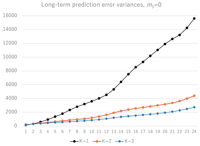
Figure 6: The long-term prediction varainces of blsallfood data for increasing prediction horaizon (i=1,…20) by the seasonal adjustment model with $m_{1}=2$, $m_{2}=1$ and $m_{3}=0$. $p$=1, 2 and 3.

We also considered the increasing-horizon prediction performance of the seasonal adjustment model with the first order trend model

$$T_{n}=T_{n-1}+u_{n},\qquad u_{n}\sim N(0,\tau^{2}).$$ (32)

Unlike the previous case of the seasonal adjustment with the second order trend model, similarly to the case of first order trend model, the increasing horaizon prediction results are almost the same for entire $p=1,\ldots 24$. However, for $p=14$ and 16, the prediction error variances are larger than other cases. It is probable that the problem of optimization cased this anomalous phenomenon.

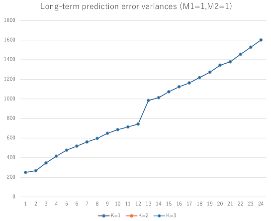
Figure 10: The long-term prediction varainces of blsallfood data for increasing prediction horaizon (i=1,…20) by the seasonal adjustment model with $m_{1}=1$ and $m_{2}=1$. NPRED=1, 2 and 3.

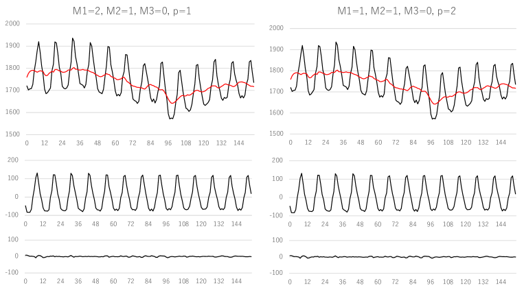
Figure 11: The seasonal adjustment with $m_{1}=1$ and $m_{2}=1$. Prediction lead time $p$=0 and 1. Top plot shows the data (black) and the mean of the trend(red), the second plot the seasonal component and the botomn plot shows the noise component.

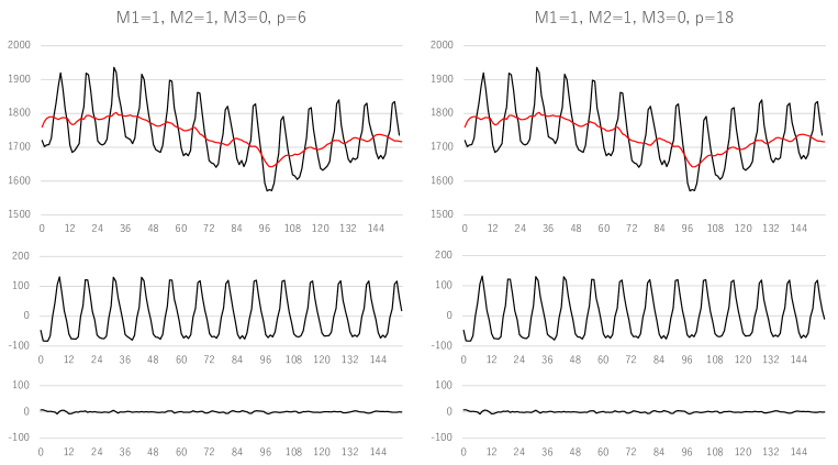
Figure 12: The seasonal adjustment model $m_{1}=1$ and $m_{2}=1$. Prediction lead time $p$=6 and 12. Top plot shows the data (black) and the mean of the trend(red), the second plot the seasonal component and the botomn plot shows the noise component.

The figures and table for this case are shown in the Appendix as Figures 10, 11, 12, and Table 3.

2.2.2 Seasonal adjustment model with AR component

Table 4 shows the long-term prediction error variances when we used the seasonal adjustment model with stationary AR component (Kitagawa and Gersch (1974), Kitagawa (2020)):

$$y_{n}=T_{n}+S_{n}+p_{n}+w_{n},$$ (33)

where $p_{n}$ is the stationary AR components that follows an AR model with order $m_{3}$,

$$p_{n}=\sum_{j=1}^{m_{3}}a_{j}y_{n-j}+z_{n},$$ (34)

$z_{n}\sim N(0,\tau^{2}_{3})$. Compared with the Table 3 for the standard seasonal adjustment model without AR component, the one-step-ahead prediction error variance is smaller and the increase of the long-term prediction error variance for large $j$ is moderate, and no noticable changes are seen by the change of the prediction horaizon $p$. The bottom row of the table shows that the minimum of the averaged prediction-error-variance is attained at $p=8\sim 20$. It can be seen that the averaged prediction error variaces are almost the same for $p=1\sim 6$, and then takes the smallest value at $p=8\sim 20$, and takes slightly larger values for $p=22$ and 24. The table also shows that, compared with the ordinary seasonal adjustment model, the seasonal adjustment model with AR component has high prediction performance over entire prediction horizon, $j=1,2,\ldots,24$.

Table 4: Long-term prediction error variances of seasonal adjustment model with $m_{1}=2$, $m_{2}=1$ and $m_{3}=2$ for various $p$.

							$p$
$j$	1	2	3	4	5	6	8	10	12	14	16	18	20	22	24
1	102	102	102	102	102	102	184	184	184	184	184	184	184	184	184
2	187	187	187	187	187	188	209	209	209	209	209	209	209	210	210
3	281	281	281	281	281	282	336	336	336	336	336	336	336	336	336
4	369	369	369	369	370	370	368	368	368	368	368	368	368	370	370
5	455	455	455	455	454	454	457	457	457	457	457	457	457	459	459
6	517	517	517	516	516	516	484	484	484	484	484	484	484	488	488
7	590	590	590	589	587	586	547	547	547	547	547	547	547	551	551
8	643	644	643	643	639	637	569	569	569	569	569	569	569	574	574
9	682	683	682	682	677	675	622	622	622	622	622	622	622	627	627
10	734	734	734	733	730	727	658	658	658	658	658	658	658	666	666
11	793	793	792	792	790	788	740	740	740	740	740	740	740	746	746
12	878	879	878	878	878	877	805	805	805	805	805	805	805	814	814
13	1002	1003	1002	1002	1002	1002	932	932	932	932	932	932	932	941	941
14	1133	1134	1133	1133	1131	1131	1003	1003	1003	1003	1003	1003	1003	1016	1016
15	1247	1248	1247	1247	1243	1243	1088	1088	1088	1088	1088	1088	1088	1102	1102
16	1349	1350	1349	1349	1344	1343	1139	1139	1139	1139	1139	1139	1139	1157	1157
17	1440	1442	1440	1440	1434	1433	1204	1204	1204	1204	1204	1204	1204	1222	1222
18	1538	1539	1538	1537	1530	1527	1258	1258	1258	1258	1258	1258	1258	1280	1280
19	1634	1635	1634	1633	1624	1621	1327	1327	1327	1327	1327	1327	1327	1349	1349
20	1737	1739	1737	1737	1727	1724	1392	1392	1392	1392	1392	1392	1392	1417	1417
21	1842	1843	1842	1841	1833	1830	1479	1479	1479	1479	1479	1479	1479	1504	1504
22	1959	1959	1958	1958	1953	1951	1569	1569	1569	1569	1569	1569	1569	1597	1597
23	2135	2136	2134	2134	2131	2128	1689	1689	1689	1689	1689	1689	1689	1717	1717
24	2359	2360	2358	2358	2352	2350	1801	1800	1800	1800	1800	1800	1800	1832	1832
	1067	1068	1067	1066	1063	1062	911	911	911	911	911	911	911	923	923

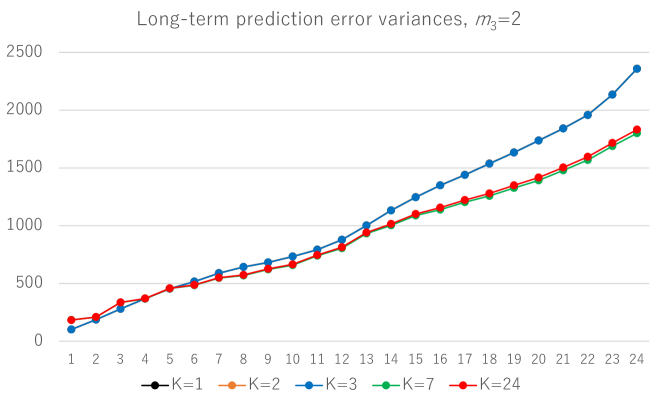
Figure 7: The long-term prediction varainces of blsallfood data for increasing prediction horaizon (i=1,…20) by the seasonal adjustment model with $m_{1}=2$, $m_{2}=1$ and $m_{3}=2$. $p$=1, 2 and 3.

Figure 7 show the long-term prediction error variances for $p=1,2,3,7$ and 24. The curves for $p=1$, 2 and 3 are visually indistinguishable. The curve for $p=24$ is slightly larger than that obtained by $p=7$.

Figure 8 shows the decomposition of the time series into the trend, sesonal component, the AR component and the observation noise obtained by $p=1$ (left plot) and $p=2$ (right plot), respectively. This suggests that by selecting a value $p$ larger than 1, it is very likely to obtain a model that has high increasing horizon prediction performance. The results are indistinguishable.

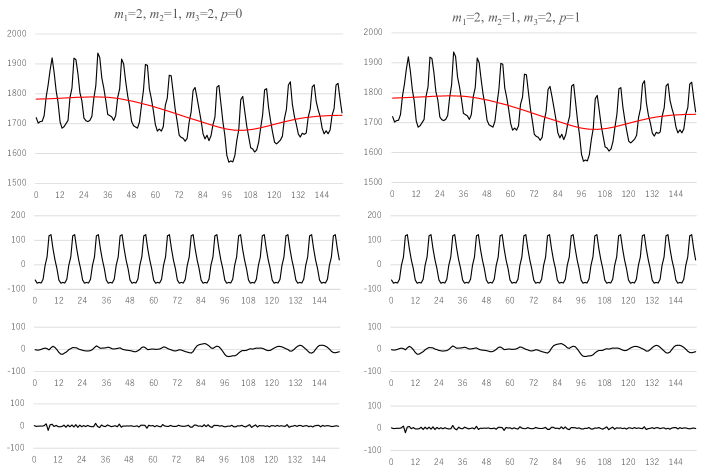
Figure 8: The seasonal adjustment with AR component $m_{1}=2$, $m_{2}=1$ and $m_{3}=2$. Prediction lead time $p$=1 and 2. Top plot shows the data (black) and the mean of the trend(red), the second plot the seasonal component, the third plot the AR component and the botomn plot shows the noise component.

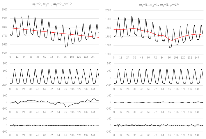
Figure 9: The seasonal adjustment with AR component $m_{1}=2$, $m_{2}=1$ and $m_{3}=2$. Prediction lead time $p$=6 and 12. Top plot shows the data (black) and the mean of the trend(red), the second plot the seasonal component, the third plot the AR component and the botomn plot shows the noise component.

On the other hand, Figure 9 shows the cases obtained by $p=6$ (left plot) and 12 (right plot). For $p=6$, the trend became a straight line and instead the AR component contains a drift. For $p=12$, the trend is slightly more variable than the trend by $p=1$ or 2 and the AR component becomes very small.

From our expectation to the trend component, these estimate obtained by $p=6$ is a bit odd. However, this estiamte has high increasing-horizon prediction performance.

3 Concluding Remarks

By the three examples, it can be seen that by specifying the prediction horizon p of the modified log-likelihood larger than 1, we can get a good long-term prediction performance. The third example suggests that the seasonal adjustment model with AR component has resonable long-term prediction performance even with $p=1$. This is probablly because the AR component can adapt to the local variation and increse the short-term prediction performance, but it does not diteriorate the long-term prediction because the prediction by stationary AR model converges to zero for large lead time.

Aknowledgements

This work was supported in part by JSPS KAKENHI Grant Number 18H03210.

Appendix: Seasonal Adjustment Model with the First Order Trend Model

Table 5: Long-term prediction error variances of the standard seasonal adjustment model with $m_{1}=1$, $m_{2}=1$.

								$p$
$j$	1	2	3	4	5	6	8	10	12	14	16	18	20	22	24
1	250	250	250	250	250	250	250	250	250	264	254	250	250	250	250
2	268	268	268	268	268	268	269	268	268	288	275	268	268	268	268
3	347	347	347	347	347	347	348	347	347	365	354	347	347	347	347
4	415	415	415	415	415	415	416	415	415	431	422	415	415	415	415
5	477	477	477	477	477	477	478	477	477	490	482	477	477	477	477
6	518	518	518	518	518	518	519	518	518	531	523	518	518	518	518
7	561	561	561	561	561	561	561	561	561	571	564	561	561	561	561
8	597	597	597	597	597	597	597	597	597	604	598	597	597	597	597
9	649	649	649	649	649	649	649	649	649	660	652	649	649	649	649
10	686	686	686	686	686	686	687	686	686	700	691	686	686	686	686
11	714	714	714	714	714	714	715	714	714	731	721	714	714	714	714
12	743	744	744	744	744	744	745	744	744	760	750	744	744	744	744
13	984	984	984	984	984	984	981	984	984	968	973	984	984	984	984
14	1012	1012	1012	1012	1012	1012	1010	1012	1012	1000	1003	1012	1012	1012	1012
15	1073	1073	1073	1073	1073	1073	1071	1073	1073	1065	1067	1073	1073	1073	1073
16	1124	1124	1124	1124	1124	1124	1123	1124	1124	1124	1121	1124	1124	1124	1124
17	1163	1163	1163	1163	1163	1163	1163	1163	1163	1173	1166	1163	1163	1163	1163
18	1218	1218	1218	1218	1218	1218	1219	1218	1218	1235	1223	1218	1218	1218	1218
19	1272	1272	1272	1272	1272	1272	1273	1272	1272	1292	1278	1272	1272	1272	1272
20	1343	1343	1343	1343	1343	1343	1344	1343	1343	1365	1350	1343	1343	1343	1343
21	1379	1379	1379	1379	1379	1379	1382	1379	1379	1415	1393	1379	1379	1379	1379
22	1455	1455	1455	1455	1455	1455	1459	1455	1455	1496	1472	1455	1455	1455	1455
23	1527	1527	1527	1527	1527	1527	1531	1527	1527	1570	1546	1527	1527	1527	1527
24	1601	1601	1601	1601	1601	1601	1604	1601	1601	1637	1616	1601	1601	1601	1601
	891	891	891	891	891	891	891	891	891	906	896	891	891	891	891

References

- [1] Akaike, H. (1974). “A new look at the statistical model identification”. IEEE transactions on automatic control, 19(6), 716–723.
- [2] Akaike, H. (1980), “Seasonal adjustment by a Bayesian modeling”, J. Time Series Anal., 1, 1–13.
- [3] Anderson, B. D. O, and Moore, J. B. (2012). Optimal filtering. DOver Publications, New York.
- [4] Judd, K., and Small, M. (2000). “Towards long-term prediction”. Physica D: Nonlinear Phenomena, 136(1-2), 31–44.
- [5] Kitagawa, G. (1989). Non-Gaussian seasonal adjustment, Computers & Mathematics with Applications, Vol.18, No.6/7, pp. 503–514.
- [6] Kitagawa, G. (2020). Introduction to Time Series Modeling with Applications in R, Monographs on Statistics and Applied Probability 166, CRD Press, Chapman & Hall, New York.
- [7] Kitagawa, G. and Gersch, W. (1984), “A smoothness priors-state space modeling of time series with trend and seasonality”, J. Amer. Statist. Assoc., 79, 378–389.
- [8] Kitagawa, G. and Gersch, W. (1996), Smoothness Priors Analysis of Time Series, Lecture Notes in Statistics, 116, Springer, New York.
- [9] Konishi, S. and Kitagawa, G. (2008), Information Criteria and Statistical Modeling, Springer Series in Statistics, pp-273, Springer, New York.
- [10] Sorjamaa, A., Hao, J., Reyhani, N., Ji, Y., and Lendasse, A. (2007). “Methodology for long-term prediction of time series”. Neurocomputing, 70(16-18), 2861–2869.
- [11] Xiong, T., Bao, Y., and Hu, Z. (2013). “Beyond one-step-ahead forecasting: evaluation of alternative multi-step-ahead forecasting models for crude oil prices”. Energy Economics, 40, 405–415.