Model-based clustering in simple hypergraphs through a stochastic blockmodel

Abstract

We propose a new model to address the overlooked problem of node clustering in simple hypergraphs. Simple hypergraphs are suitable when a node may not appear multiple times in the same hyperedge, such as in co-authorship datasets. Our model assumes the existence of latent node groups and hyperedges are conditionally independent given these groups. We first establish the generic identifiability of the model parameters. We then develop a variational approximation Expectation-Maximization algorithm for parameter inference and node clustering, and derive a statistical criterion for model selection.

To illustrate the performance of our R package HyperSBM, we compare it with other node clustering methods using synthetic data generated from the model, as well as from a line clustering experiment and a co-authorship dataset. As a by-product, our synthetic experiments demonstrate that the detectability thresholds for non-uniform sparse hypergraphs cannot be deduced from the uniform case.

Keywords: high-order interactions, Kesten-Stigum threshold, latent variable model, line clustering, non-uniform hypergraph, variational expectation-maximization.

1 Introduction

Over the past two decades, a wide range of models has been developed to capture pairwise interactions represented in graphs. However, modern applications in various fields have highlighted the necessity to consider high-order interactions, which involve groups of three or more nodes. Simple examples include triadic and larger group interactions in social networks (whose importance has been recognized early on, see Simmel, 1950), scientific co-authorship (Estrada and Rodríguez-Velázquez, 2006), interactions among more than two species in ecological systems (Muyinda et al., 2020; Singh and Baruah, 2021), or high-order correlations between neurons in brain networks (Chelaru et al., 2021). To formalize these high-order interactions, hypergraphs provide the most general framework. Similar to a graph, a hypergraph consists of a set of nodes and a set of hyperedges, where each hyperedge is a subset of nodes involved in an interaction.

In this context, it is important to distinguish simple hypergraphs from multiset hypergraphs, where hyperedges can contain repeated nodes. Multisets are a generalization of sets, allowing elements to appear with varying multiplicities. Recent reviews on high-order interactions can be found in the works of Battiston et al. (2020), Bick et al. (2021), and Torres et al. (2021).

Despite the increasing interest in high-order interactions, the statistical literature on this topic remains limited. Some graph-based statistics, such as centrality or clustering coefficient, have been extended to hypergraphs to aid in understanding the structure and extracting information from the data (Estrada and Rodríguez-Velázquez, 2006). However, these statistics do not fulfill the need for random hypergraph models.

Early analyses of hypergraphs have relied on their embedding into the space of bipartite graphs (see, e.g., Battiston et al., 2020). Hypergraphs with self-loops and multiple hyperedges (weighted hyperedges with integer-valued weights) are equivalent to bipartite graphs. However, bipartite graph models were not specifically designed for hypergraphs and may introduce artifacts (please refer to Section A in the Supplementary Material for more details).

Generalizing Erdős-Rényi’s model of random graphs leads to uniformly random hypergraphs. This model involves drawing uniformly at random from the set of all $m$-uniform hypergraphs (hypergraphs with hyperedges of fixed cardinality $m$) over a set of $n$ nodes. However, similar to Erdős-Rényi’s model for graphs, this hypergraph model is too simplistic and homogeneous to be used for statistical analysis of real-world datasets. In the configuration model for random graphs, the graphs are generated by drawing uniformly at random from the set of all possible graphs over a set of $n$ nodes, while satisfying a given prescribed degree sequence. In the context of hypergraphs, configuration models were proposed in Ghoshal et al. (2009), focusing on tripartite and 3-uniform hypergraphs. Later, Chodrow (2020) extended the configuration model to a more general hypergraph setup. In these references, both the node degrees and the hyperedge sizes are kept fixed (a consequence of the fact that they rely on bipartite representations of hypergraphs). The configuration model is useful for sampling (hyper)graphs with the same degree sequence (and hyperedge sizes) as an observed dataset through shuffling algorithms. Therefore, it is often employed as a null model in statistical analyses. However, sampling exactly (rather than approximately) from this model poses challenges, particularly in the case of hypergraphs. For a comprehensive discussion on this issue, we refer readers to Section 4 in Chodrow (2020).

Another popular approach for extracting information from heterogeneous data is clustering. In the context of graphs, stochastic blockmodels (SBMs) were introduced in the early eighties (Frank and Harary, 1982; Holland et al., 1983) and have since evolved in various directions. These models assume that nodes are grouped into clusters, and the probabilities of connections between nodes are determined by their cluster memberships. Variants of SBMs have been developed to handle weighted graphs and degree-corrected versions, among others. In the context of hypergraphs, Ghoshdastidar and Dukkipati (2014) introduced a planted partition model for $m$-uniform hypergraphs, which is a specific case of SBM. They developed a spectral partitioning method and established its consistency in the case where nodes are grouped into equally-sized clusters, and two parameters determine the connection probabilities within clusters and between clusters, with the former being larger than the latter. This result was further extended to the non-uniform and weighted sparse setting, where most weights are close to zero, in Ghoshdastidar and Dukkipati (2017). By introducing hypergraphons, Balasubramanian (2021) extended the ideas of hypergraph SBMs to a nonparametric setting. In a parallel vein, Turnbull et al. (2021) proposed a latent space model for hypergraphs, generalizing random geometric graphs to hypergraphs, although it was not specifically designed to capture clustering. An approach linked to SBMs is presented in Vazquez (2009), where nodes belong to latent groups and participate in a hyperedge with a probability that depends on both their group and the specific hyperedge.

Modularity is a widely used criterion for clustering entities in the context of interaction data. It aims to identify specific clusters, known as communities, characterized by high within-group connection probabilities and low between-group connection probabilities (Ghoshdastidar and Dukkipati, 2014). However, in the hypergraph context, the definition of modularity is not unique. In particular, Kamiński et al. (2019) introduced a “strict” modularity criterion, where only hyperedges with all their nodes belonging to the same group contribute to an increase in modularity. Their criterion measures the deviation of the number of these homogeneous hyperedges from a new null model called the configuration-like model for hypergraphs, where the average values of the degrees are fixed. Building upon this, Chodrow et al. (2021) proposed a degree-corrected hypergraph SBM and introduced two new modularity criteria. Similar to Kamiński et al. (2019), one of these criteria utilizes an “all-or-nothing” affinity function that distinguishes whether a given hyperedge is entirely contained within a single cluster or not. In this setup, they established a connection between approximate maximum likelihood estimation and their modularity criterion. This work is reminiscent of the work of Newman (2016) in the graph context. However, the estimators proposed by Chodrow et al. (2021) do not guarantee maximum likelihood estimation, as they constrained the parameter space by assuming a symmetric affinity function.

It is important to highlight that the developments presented in Kamiński et al. (2019) and Chodrow et al. (2021) are specifically conducted in the context of multiset hypergraphs, where hyperedges can contain repeated nodes with certain multiplicities. The use of multiset hypergraphs simplifies some of the challenges associated with computing modularity. However, to the best of our knowledge, modularity approaches still lack instantiation in the case of simple hypergraphs where each node can only appear once in a hyperedge. More specifically, the null model used in hypergraph modularity criteria relies on a model for multiset hypergraphs, similar to how the null model used in classical graph modularity is based on graphs with self-loops. While it is known in the case of graphs that this assumption is inadequate, as it induces a stronger deviation than expected and affects sparse networks as well (Massen and Doye, 2005; Cafieri et al., 2010; Squartini and Garlaschelli, 2011), the assumption of multisets has not yet been discussed in the context of hypergraph modularity.

In the context of community detection, random walk approaches have also been utilized for hypergraph clustering (Swan and Zhan, 2021). Additionally, low-rank tensor decompositions have been explored (Ke et al., 2020). The misclassification rate for the community detection problem in hypergraphs and its limits have been analyzed in various contexts (see, for instance, Ahn et al., 2018; Chien et al., 2019; Cole and Zhu, 2020). It is worth mentioning that a recent approach has been proposed to cluster hyperedges instead of nodes (Ng and Murphy, 2022). However, our focus in this work is on clustering nodes.

The literature on high-order interactions often discusses simplicial complexes alongside hypergraphs (Battiston et al., 2020). However, the unique characteristic of simplicial complexes, where each subset of an occurring interaction should also occur, places them outside the scope of this introduction, which is specifically focused on hypergraphs.

In this article, our focus is on model-based clustering for simple hypergraphs, specifically studying stochastic hypergraph blockmodels. We formulate a general stochastic blockmodel for simple hypergraphs, along with various submodels, and outline the key differences compared to previous proposals (Section 2.1). We provide the first result on the generic identifiability of parameters in a hypergraph stochastic blockmodel (Section 2.2). Parameter inference and node clustering are performed using a variational Expectation-Maximization (VEM) algorithm (Section 2.3) that approximates the maximum likelihood estimator. Model selection for the number of groups is based on an integrated classification likelihood (ICL) criterion (Section 2.4). To illustrate the performance of our method, we conduct experiments on synthetic sparse hypergraphs, including a comparison with hypergraph spectral clustering (HSC) and modularity approaches (Section 3). Notably, the line clustering experiment (Section 3.4) highlights the significant differences between our approach and the one proposed by Chodrow et al. (2021). As a by-product, our synthetic experiments demonstrate that the detectability thresholds for non-uniform sparse hypergraphs, also known as Kesten-Stigum thresholds (Angelini et al., 2015; Stephan and Zhu, 2022) cannot be deduced from the uniform case (Section 3.2). We also analyze a co-authorship dataset, presenting conclusions that differ from spectral clustering and bipartite stochastic blockmodels (Section 4). The proofs of all theoretical results are provided in Section 5. An R package, HyperSBM, which implements our method in efficient C++ code, as well as all associated scripts, are available online (see Section 6). This manuscript is accompanied by Supplementary Material (SM) that contains additional information and experiments.

2 A stochastic blockmodel for hypergraphs

2.1 Model formulation

Let $\mathcal{H}=(\mathcal{V},\mathcal{E})$ represent a binary hypergraph, where $\mathcal{V}=\{1,\dots,n\}$ is a set of $n$ nodes and $\mathcal{E}$ is the set of hyperedges. In this context, a hyperedge of size $m\geq 2$ is defined as a collection of $m$ distinct nodes from $\mathcal{V}$. We do not allow for hyperedges to be multisets or self-loops. Let $M=\underset{e\in\mathcal{E}}{\max}|e|$ denote the largest possible size of hyperedges in $\mathcal{E}$, with $M\geq 2$ (for graphs, $M=2$). We can define the sets of node subsets, node tuples, and hyperedges of size $m$ as

$$\mathcal{V}^{(m)} =\big{\{}\{i_{1},\dots,i_{m}\}:i_{1},\dots,i_{m}\in\mathcal{V}\text{ are all distinct}\big{\}},$$

$$\mathcal{V}^{m} =\big{\{}(i_{1},\dots,i_{m}):i_{1},\dots,i_{m}\in\mathcal{V}\text{ are all distinct}\big{\}},$$

$$\mathcal{E}^{(m)} =\big{\{}\{i_{1},\dots,i_{m}\}\in\mathcal{V}^{(m)}:\{i_{1},\dots,i_{m}\}\in\mathcal{E}\big{\}},$$

respectively. Obviously $\mathcal{E}=\bigcup_{m=2}^{M}\mathcal{E}^{(m)}\subseteq\bigcup_{m=2}^{M}\mathcal{V}^{(m)}$. For each node subset $\{i_{1},\dots,i_{m}\}\in\mathcal{V}^{(m)}$, we can define the indicator variable:

$$Y_{i_{1},\dots,i_{m}}=\mathbbm{1}_{\{i_{1},\dots,i_{m}\}\in\mathcal{E}}=\begin{cases}1\qquad&\text{if }\{i_{1},\dots,i_{m}\}\in\mathcal{E},\\ 0&\text{if }\{i_{1},\dots,i_{m}\}\notin\mathcal{E}.\end{cases}$$

We can represent a random hypergraph as $\bm{Y}=(Y_{i_{1},\dots,i_{m}})_{{i_{1},\dots,i_{m}}\in\mathcal{V}^{(m)}}$.

Similar to the formulation of the stochastic blockmodel (SBM) for graphs, we assume that the nodes in the hypergraph belong to $Q$ unobserved groups. We use $Z_{1},\dots,Z_{n}$ to denote $n$ independent and identically distributed latent variables, where $Z_{i}$ follows a prior distribution $\pi_{q}=\mathbb{P}(Z_{i}=q)$ for each $q=1,\dots,Q$. The values $\pi_{q}$ satisfy $\pi_{q}\geq 0$ and $\sum_{q=1}^{Q}\pi_{q}=1$. To simplify notation, we sometimes represent $Z_{i}$ as a binary vector $Z_{i}=(Z_{i1},\dots,Z_{iQ})\in\{0,1\}^{Q}$, where only one element, $Z_{iq}$, equals 1. We also define $\bm{Z}=(Z_{1},\dots,Z_{n})$. For every $m$-subset of nodes, we associate a latent configuration that represents the set of latent groups to which these nodes belong. We define

$$\mathcal{Q}^{(m)}=\big{\{}\{q_{1},\dots,q_{m}\}:q_{1},\dots,q_{m}\in\{1,\dots,Q\}\big{\}},$$

as the set of all possible latent configurations for elements in $\mathcal{V}^{(m)}$. Note that the values of the latent groups within a configuration may be repeated. Now, given the latent variables $\bm{Z}$, all indicator variables $Y_{i_{1},\dots,i_{m}}$ are assumed to be independent and follow a Bernoulli distribution whose parameter depends on the latent configuration:

$$Y_{i_{1},\dots,i_{m}}|\{Z_{1}=q_{1},\dots,Z_{m}=q_{m}\}\sim\mathcal{B}(B^{(m,n)}_{q_{i_{1}},\dots,q_{i_{m}}}),\qquad\text{ for any }\{i_{1},\dots,i_{m}\}\in\mathcal{V}^{(m)}.$$

Here $B^{(m,n)}_{q_{1},\dots,q_{m}}$ represents the probability that $m$ unordered nodes, with latent configuration $\{q_{1},\dots,q_{m}\}$, are connected into a hyperedge. We emphasize the dependency of those parameters on both $m$ and $n$, having in mind 2 possible sparse settings. First, as the number of nodes increases, it is natural to assume that the probability of a hyperedge may decrease; otherwise, we would only observe dense hypergraphs. Second, while it is implicit that $B^{(m,n)}_{q_{1},\dots,q_{m}}$ depends on $m$ through $q_{1},\dots,q_{m}$, we emphasize this dependency as it is likely that real data contain fewer hyperedges of larger size $m$. Each $B^{(m,n)}$ is a fully symmetric tensor of rank $m$, namely

$$B^{(m,n)}_{q_{1},\dots,q_{m}}=B^{(m,n)}_{q_{\sigma(1)},\dots,q_{\sigma(m)}},\ \forall q_{1},\dots,q_{m}\text{ and }\forall\sigma\text{ permutation of }\{1,\dots,m\}.$$ (1)

We denote the parameter vector as $\theta=(\pi_{q},B^{(m,n)}_{q_{1},\dots,q_{m}})_{q,m,q_{1}\leq\dots\leq q_{m}}$ and the corresponding probability distribution and expectation as $\mathbb{P}_{\theta},\mathbb{E}_{\theta}$, respectively.

Lemma 1.

The number of different parameters in each tensor $B^{(m,n)}=(B^{(m,n)}_{q_{1},\dots,q_{m}})_{1\leq q_{1}\leq\dots\leq q_{m}\leq Q}$ is $\binom{Q+m-1}{m}$.

As a result, the total number of parameters in our hypergraph stochastic blockmodel (HSBM) is given by:

$$(Q-1)+\sum_{m=2}^{M}\binom{Q+m-1}{m}.$$

As shown in Table 1, the number of $B^{(m,n)}_{q_{1},\dots,q_{m}}$ parameters increases rapidly as the values of $Q$ and $m$ grow. To reduce the complexity of the model, we introduce submodels by assuming equality of certain conditional probabilities $B^{(m,n)}_{q_{1},\dots,q_{m}}$. In particular, we consider two affiliation submodels given by

$$B^{(m,n)}_{q_{1},\dots,q_{m}}=\begin{cases}\alpha^{(m,n)}\quad\text{if }q_{1}=\dots=q_{m},\\ \beta^{(m,n)}\quad\text{if there exist at least }q_{i}\neq q_{j}\text{ for }i\neq j\end{cases}$$ (Aff-m)

and

$$B^{(m,n)}_{q_{1},\dots,q_{m}}=\begin{cases}\alpha^{(n)}\quad\text{if }q_{1}=\dots=q_{m}\\ \beta^{(n)}\quad\text{if there exist at least }q_{i}\neq q_{j}\text{ for }i\neq j\end{cases}\forall m=2,\dots,M.$$ (Aff)

The number of parameters is dropped to $(Q-1)+2(M-1)$ and to $(Q-1)+2$ under Assumptions (Aff-m) and (Aff), respectively. These submodels align with the concepts discussed in Kamiński et al. (2019) and Chodrow et al. (2021), where they propose that only hyperedges with nodes belonging to the same group should contribute to the increase in modularity. Additionally, these submodels correspond to the scenarios in which Ghoshdastidar and Dukkipati (2014, 2017) obtained their results.

	$Q$
$m$	2	3	4	5	6	7
3	4	10	20	35	56	84
4	5	15	35	70	126	210
5	6	21	56	126	252	462
6	7	28	84	210	462	924
7	8	36	120	330	792	1716

Table 1: Number $\binom{Q+m-1}{m}$ of connectivity parameters $B^{(m,n)}_{q_{1},\dots,q_{m}}$ of the full HSBM for given values of $Q$ (number of latent groups) and $m$ (hyperedge size).

Generalizations.

Our model can accommodate self-loops without significant changes by allowing for $m=1$. Furthermore, it can be easily extended to handle multiple hypergraphs (with or without self-loops) by incorporating a zero-inflated or deflated Poisson distribution on the conditional distribution of the hyperedges. In a more general setting, the conditional Bernoulli distribution can be replaced with any parametric distribution to handle weighted hypergraphs, and it could also easily incorporate covariates. This flexibility allows for the adaptation of our model to various types of hypergraph data.

Distinction from previous proposals.

We here highlight the distinctive methodological aspects of our approach compared to other existing methods. Ghoshdastidar and Dukkipati (2014, 2017) obtained error bounds that converge to zero only for specific cases of the (Aff-m) model with equally-sized groups. Their results are limited to these specific scenarios, whereas our approach extends beyond such constraints. References such as Ke et al. (2020); Ahn et al. (2018); Chien et al. (2019) primarily focus on community detection, which means they only identify clusters that correspond to communities. In contrast, our method is not limited to detecting community-like structures, but can find clusters that may not align with traditional notions of communities (e.g. disassortative clusters). Chodrow et al. (2021) introduced a comprehensive degree-corrected SBM for multiple hypergraphs. However, their inference method solves the clustering problem in the space of multiset hypergraphs, whereas our approach is specifically designed for simple hypergraphs. While both models are valid, they lead to different statistical analyses, and the choice of which model to use depends on the specific characteristics of the data. Furthermore, it is worth noting that while Chodrow et al. (2021) initially employ a maximum likelihood approach, they deviate from that setting during their analysis. In contrast, our method retains the maximum likelihood framework throughout the inference process. Lastly, the SBM for hypergraphs presented in Balasubramanian (2021) is highly general. However, their least-squares estimator for a hypergraphon model is computationally infeasible. Additionally, their Algorithm 1 is dedicated to community detection and does not provide general cluster recovery.

In Sections 3 and 4, we provide numerical illustrations that highlight the differences between our algorithm and those proposed by Chodrow et al. (2021); Kamiński et al. (2019); Ghoshdastidar and Dukkipati (2017), as well as the bipartite SBM.

2.2 Parameter identifiability

We first establish the generic identifiability of the parameters in a HSBM that is restricted to simple $m$-uniform hypergraphs for any $m\geq 2$. In a parametric context, generic identifiability implies that every parameter $\theta$, except possibly for some parameters in a subset of dimension strictly smaller than the full parameter space, uniquely determines the distribution $\mathbb{P}_{\theta}$. In other words, if we randomly select a parameter $\theta\in\Theta$ according to the Lebesgue measure, it almost surely uniquely defines $\mathbb{P}_{\theta}$. Identifiability is established up to label switching on the node groups, as is common in discrete latent variable models. For the case of $m=2$, the identifiability result corresponds to Theorem 2 in Allman et al. (2011). Our proof follows similar principles, building upon a key result by Kruskal (1977). In our case, we crucially additionally rely on a sufficient condition for a sequence of nonnegative integers to represent the degree sequence of a simple $m$-uniform hypergraph, as established by Behrens et al. (2013).

Theorem 2.

For any $m\geq 2$ and any integer $Q$, the parameter $\theta=(\pi_{q},B^{(m,n)}_{q_{1},\dots,q_{m}})_{1\leq q\leq Q,1\leq q_{1}\leq\dots\leq q_{m}\leq Q}$ of the HSBM restricted to $m$-uniform simple hypergraphs over $n$ nodes, is generically identifiable, up to label switching on the node groups, for large enough $n$ (depending only on $m,Q$).

This result does not provide specific insights into the identifiability when we restrict the model to fixed group proportions, such as equal group proportions $\pi_{q}=1/Q$. Indeed, it does not explicitly characterize the subspace of the parameter space where identifiability may not hold, although we know that its dimension is smaller than that of the full parameter space. When we impose fixed group proportions, we are precisely working within a lower-dimensional subspace, and identifiability may not be guaranteed without additional considerations.

Similarly, this result says nothing about the affiliation cases (Aff-m) and (Aff), which correspond to further restrictions of the parameter space to lower-dimensional subspaces.

The result we have established for $m$-uniform hypergraphs also implies a similar result for non-uniform simple hypergraphs, as shown in the following corollary.

Corollary 3.

For any integer $Q$, the parameter $\theta=(\pi_{q},B^{(m,n)}_{q_{1},\dots,q_{m}})_{1\leq q\leq Q,1\leq q_{1}\leq\dots\leq q_{m}\leq Q,2\leq m\leq M}$ of the HSBM for simple hypergraphs over $n$ nodes is generically identifiable, up to label switching on the node groups, for large enough $n$ (depending only on $M,Q$).

Our proof of Corollary 3 relies on the assumption that all the $\pi_{q}$’s are distinct, which is a generic condition. This condition is not explicitly stated in the corollary, but it is required for the proof to hold. Consequently, the result of generic identifiability does not bring any insight in cases where the group proportions are equal, as it is not sufficient to identify the parameters separately for each value of $m$.

Additional technical work is thus needed to establish whether a HSBM with equal group proportions, or whether the affiliation submodels have identifiable parameters.

2.3 Parameter estimation via variational Expectation-Maximization

The likelihood of the model is given by

$$\mathbb{P}_{\theta}(\bm{Y}) =\sum_{q_{1}=1}^{Q}\dots\sum_{q_{n}=1}^{Q}\mathbb{P}_{\theta}(\bm{Y},\bm{Z}=(q_{1},\dots,q_{n}))$$

$$=\sum_{q_{1}=1}^{Q}\dots\sum_{q_{n}=1}^{Q}\left(\prod_{i=1}^{n}\mathbb{P}_{\theta}(Z_{i}=q_{i})\right)\prod_{m=2}^{M}\prod_{\{i_{1},\dots,i_{m}\}\in\mathcal{V}^{(m)}}\mathbb{P}_{\theta}(Y_{i_{1},\dots,i_{m}}|Z_{i_{1}}=q_{i_{1}},\dots,Z_{i_{m}}=q_{i_{m}})$$

$$=\sum_{q_{1}=1}^{Q}\dots\sum_{q_{n}=1}^{Q}\left(\prod_{i=1}^{n}\pi_{q_{i}}\right)\prod_{m=2}^{M}\prod_{\{i_{1},\dots,i_{m}\}\in\mathcal{V}^{(m)}}(B^{(m,n)}_{q_{i_{1}},\dots,q_{i_{m}}})^{Y_{i_{1},\dots,i_{m}}}(1-B^{(m,n)}_{q_{i_{1}},\dots,q_{i_{m}}})^{1-Y_{i_{1},\dots,i_{m}}}.$$ (2)

The computation of the model likelihood is generally intractable. Equation (2.3) involves a summation over all possible $Q^{n}$ different latent configurations, which becomes computationally prohibitive when $n$ and $Q$ are large. In the context of latent variable models, the Expectation-Maximization (EM) algorithm (Dempster et al., 1977) is commonly used to address this issue. However, the EM algorithm cannot be directly applied to SBMs. This is because the E-step, which involves computing the conditional posterior distribution of the latent variables $P(\bm{Z}|\bm{Y})$, is itself intractable in SBMs (see, e.g., Matias and Robin, 2014). One possible solution is to employ variational approximations of the EM algorithm, known as Variational EM (VEM Jordan et al., 1999).

We let

$$f(y,b):=y\log b+(1-y)\log b.$$ (3)

Then, the complete data log-likelihood is

$$\ell_{n}^{c}(\theta) =\log\mathbb{P}_{\theta}(\bm{Y},\bm{Z})=\log\mathbb{P}_{\theta}(\bm{Z})+\log\mathbb{P}_{\theta}(\bm{Y}|\bm{Z})$$ (4)

$$=\sum_{q=1}^{Q}\sum_{i=1}^{n}Z_{iq}\log\pi_{q}+\sum_{m=2}^{M}\sum_{q_{1}=1}^{Q}\dots\sum_{q_{m}=1}^{Q}\sum_{\{i_{1},\dots,i_{m}\}\in\mathcal{V}^{(m)}}Z_{i_{1}q_{1}}\cdots Z_{i_{m}q_{m}}f(Y_{i_{1}\dots i_{m}},B^{(m,n)}_{q_{1},\dots,q_{m}})$$

$$=\sum_{q=1}^{Q}\sum_{i=1}^{n}Z_{iq}\log\pi_{q}+\sum_{m=2}^{M}\sum_{q_{1}\leq q_{2}\leq\dots\leq q_{m}}\sum_{(i_{1},\dots,i_{m})\in\mathcal{V}^{m}}Z_{i_{1}q_{1}}\cdots Z_{i_{m}q_{m}}f(Y_{i_{1}\dots i_{m}},B^{(m,n)}_{q_{1},\dots,q_{m}}).$$

Note that the final equality ensures that each parameter value appears only once. The key principle underlying the variational method is to adopt the same iterative two-step structure as the EM algorithm but replace the intractable posterior distribution $\mathbb{P}_{\theta}(\bm{Z}|\bm{Y})$ with the best approximation, in terms of Kullback-Leibler divergence, from a class of simpler distributions, often factorized. We introduce a class of factorized probability distributions $\mathbb{Q}_{\tau}$ over $\bm{Z}=(Z_{1},\dots,Z_{n})$ given by

$$\mathbb{Q}_{\tau}(\bm{Z})=\prod_{i=1}^{n}\mathbb{Q}_{\tau}(Z_{i})=\prod_{i=1}^{n}\prod_{q=1}^{Q}\tau_{iq}^{Z_{iq}},$$

where the variational parameter $\tau_{iq}=\mathbb{Q}_{\tau}(Z_{i}=q)\in[0,1]$ and $\sum_{q=1}^{Q}\tau_{iq}=1$ for any $i=1,\dots,n$ and $q=1,\dots,Q$. The expectation under distribution $\mathbb{Q}_{\tau}$ is denoted as $\mathbb{E}_{\mathbb{Q}_{\tau}}$, and $\mathcal{H}(\mathbb{Q}_{\tau})$ represents the entropy of $\mathbb{Q}_{\tau}$. Now we define the evidence lower bound (ELBO):

$$\mathcal{J}(\theta,\tau) =\mathbb{E}_{\mathbb{Q}_{\tau}}[\log\mathbb{P}_{\theta}(\bm{Y},\bm{Z})]+\mathcal{H}(\mathbb{Q}_{\tau})$$ (5)

$$=\mathbb{E}_{\mathbb{Q}_{\tau}}[\log\mathbb{P}_{\theta}(\bm{Y},\bm{Z})]-\mathbb{E}_{\mathbb{Q}_{\tau}}[\log\mathbb{Q}_{\tau}(\bm{Z})]$$

$$=\sum_{q=1}^{Q}\sum_{i=1}^{n}\tau_{iq}\log\frac{\pi_{q}}{\tau_{iq}}+\sum_{m=2}^{M}\sum_{q_{1}\leq q_{2}\leq\dots\leq q_{m}}\sum_{(i_{1},\dots,i_{m})\in\mathcal{V}^{m}}\tau_{i_{1}q_{1}}\cdots\tau_{i_{m}q_{m}}f(Y_{i_{1}\dots i_{m}},B^{(m,n)}_{q_{1},\dots,q_{m}}).$$

It can be observed that $\mathcal{J}(\theta,{\tau})$ satisfies the following relation:

$$\mathcal{J}({\theta},{\tau})=\log\mathbb{P}_{\theta}(\bm{Y})-\text{KL}(\mathbb{Q}_{\tau}(\bm{Z})||\mathbb{P}_{\theta}(\bm{Z}|\bm{Y})),$$ (6)

where $\text{KL}(\cdot||\cdot)$ denotes the Kullback-Leibler divergence. Thus, $\mathcal{J}$ serves as a lower bound for the model log-likelihood $\log\mathbb{P}_{\theta}(\bm{Y})$. The VEM algorithm iterates between the following two steps until a suitable convergence criterion is met:

• VE-Step maximizes $\mathcal{J}({\theta},{\tau})$ with respect to ${\tau}$

  $$\widehat{{\tau}}^{(t)}=\underset{{\tau}}{\arg\max}\ \mathcal{J}({\theta}^{(t-1)},{\tau}),\quad\text{s.t. }\textstyle\sum_{q=1}^{Q}\widehat{\tau}^{(t)}_{iq}=1\qquad\forall i=1,\dots,n.$$ (7)

  This step involves finding the best approximation of the conditional distribution $\mathbb{P}_{\theta}(\bm{Z}|\bm{Y})$ by minimizing the Kullback-Leibler divergence term in (6).

• M-Step maximizes $\mathcal{J}({\theta},{\tau})$ with respect to ${\theta}$

  $$\widehat{{\theta}}^{(t)}=\underset{{\theta}}{\arg\max}\ \mathcal{J}({\theta},{\tau}^{(t-1)}),\quad\text{s.t. }\textstyle\sum_{q=1}^{Q}\widehat{\pi}^{(t)}_{q}=1.$$ (8)

  This step updates the values of the model parameters $\pi_{q}$ and $B^{(m,n)}_{q_{1},\dots,q_{m}}$.

In the following we provide the solutions of the two maximization problems in Equations (7) and (8).

Proposition 4 (VE-Step).

Given the current model parameters $(\pi_{q},B^{(m,n)}_{q_{1},\dots,q_{m}})_{q,m,q_{1},\dots,q_{m}}$ at any iteration of the VEM algorithm, the corresponding optimal values of the variational parameters $(\widehat{\tau}_{iq})_{i,q}$ defined in Equation (7) should satisfy the fixed point equation:

$$\log\widehat{\tau}_{iq}=\log\pi_{q}+\sum_{m=1}^{M-1}\sum_{q_{1}\leq q_{2}\leq\dots\leq q_{m}}\sum_{\begin{subarray}{c}(i_{1},\dots,i_{m})\in\mathcal{V}^{m}\\ \text{s.t.}\{i,i_{1},\dots,i_{m}\}\in\mathcal{V}^{(m+1)}\end{subarray}}\widehat{\tau}_{i_{1}q_{1}}\cdots\widehat{\tau}_{i_{m}q_{m}}f(Y_{ii_{1}\dots i_{m}},B^{(m+1,n)}_{qq_{1}\dots q_{m}})+c_{i},$$ (9)

for any $1\leq i\leq n$ and $1\leq q\leq Q$ and where $c_{i}$ are normalising constants such that $\sum_{q}\widehat{\tau}_{iq}=1$.

Remark.

From Proposition 4, the $\tau_{i}$’s are obtained using a fixed point algorithm. Although in all the situations we experienced, the algorithm converged in a reasonable number of iterations, we have no guarantee about existence nor uniqueness of a solution to (9).

Proposition 5 (M-Step).

Given the variational parameters $(\tau_{iq})_{i,q}$ at any iteration of the VEM algorithm, the corresponding optimal values of the model parameters $(\widehat{\pi}_{q},\widehat{B}^{(m,n)}_{q_{1}\dots q_{m}})_{q,m,q_{1}\leq\dots\leq q_{m}}$ defined in Equation (8) are given by

$$\widehat{\pi}_{q}=\frac{1}{n}\sum_{i=1}^{n}\tau_{iq}\qquad\text{ and }\qquad\widehat{B}^{(m,n)}_{q_{1}\dots q_{m}}=\frac{\sum_{(i_{1},\dots,i_{m})\in\mathcal{V}^{m}}\tau_{i_{1}q_{1}}\dots\tau_{i_{m}q_{m}}Y_{i_{1}\dots i_{m}}}{\sum_{(i_{1},\dots,i_{m})\in\mathcal{V}^{m}}\tau_{i_{1}q_{1}}\dots\tau_{i_{m}q_{m}}}.$$

We now express the solutions of the M-Step under the submodels given by (Aff-m) and (Aff). Note that the VE-Step is unchanged under these settings.

Proposition 6 (M-Step, affiliation setup).

In the particular affiliations submodels given by (Aff-m) and (Aff) respectively, given variational parameters $(\tau_{iq})_{i,q}$, at any iteration of the VEM algorithm, the corresponding optimal values of $(\widehat{\alpha}^{(m,n)},\widehat{\beta}^{(m,n)})_{m}$ and $\widehat{\alpha^{(n)}},\widehat{\beta^{(n)}}$ maximising $\mathcal{J}$ as in Equation (8) are given by

• Under Assumption (Aff-m),

  $$\widehat{\alpha}^{(m,n)} =\frac{\sum_{q=1}^{Q}\sum_{i_{1}<\dots<i_{m}}\tau_{i_{1}q}\dots\tau_{i_{m}q}Y_{i_{1}\dots i_{m}}}{\sum_{q=1}^{Q}\sum_{i_{1}<\dots<i_{m}}\tau_{i_{1}q}\dots\tau_{i_{m}q}},$$

  $$\widehat{\beta}^{(m,n)} =\frac{\sum_{\begin{subarray}{c}q_{1}\leq\dots\leq q_{m}\\ |\{q_{1},\dots,q_{m}\}|\geq 2\end{subarray}}\sum_{(i_{1},\dots,i_{m})\in\mathcal{V}^{m}}\tau_{i_{1}q_{1}}\dots\tau_{i_{m}q_{m}}Y_{i_{1}\dots i_{m}}}{\sum_{\begin{subarray}{c}q_{1}\leq\dots\leq q_{m}\\ |\{q_{1},\dots,q_{m}\}|\geq 2\end{subarray}}\sum_{(i_{1},\dots,i_{m})\in\mathcal{V}^{m}}\tau_{i_{1}q_{1}}\dots\tau_{i_{m}q_{m}}}.$$

• Under Assumption (Aff),

  $$\widehat{\alpha^{(n)}} =\frac{\sum_{m=2}^{M}\sum_{q=1}^{Q}\sum_{i_{1}<\dots<i_{m}}\tau_{i_{1}q}\dots\tau_{i_{m}q}Y_{i_{1}\dots i_{m}}}{\sum_{m=2}^{M}\sum_{q=1}^{Q}\sum_{i_{1}<\dots<i_{m}}\tau_{i_{1}q}\dots\tau_{i_{m}q}},$$

  $$\widehat{\beta^{(n)}} =\frac{\sum_{m=2}^{M}\sum_{\begin{subarray}{c}q_{1}\leq\dots\leq q_{m}\\ |\{q_{1},\dots,q_{m}\}|\geq 2\end{subarray}}\sum_{(i_{1},\dots,i_{m})\in\mathcal{V}^{m}}\tau_{i_{1}q_{1}}\dots\tau_{i_{m}q_{m}}Y_{i_{1}\dots i_{m}}}{\sum_{m=2}^{M}\sum_{\begin{subarray}{c}q_{1}\leq\dots\leq q_{m}\\ |\{q_{1},\dots,q_{m}\}|\geq 2\end{subarray}}\sum_{(i_{1},\dots,i_{m})\in\mathcal{V}^{m}}\tau_{i_{1}q_{1}}\dots\tau_{i_{m}q_{m}}}.$$

Algorithm initialization.

We choose to begin the algorithm with its M-step, which provides an initial value for $\bm{\tau}$. This allows us to leverage smart initialization strategies based on a preliminary clustering of the nodes. Specifically, we employ three different initialization strategies and select the best result that maximizes the ELBO criterion $\mathcal{J}$:

Random initialization: This naive method involves drawing each $(\tau_{iq})_{1\leq q\leq Q}$ uniformly from $(0,1)$ for every node $i$ and normalizing the vector $\tau_{i}$.

“Soft” spectral clustering: We utilize Algorithm 1 from Ghoshdastidar and Dukkipati (2017) combined with soft $k$-means. In this approach, we compute a hypergraph Laplacian and construct the column matrix $X$ consisting of its leading $Q$ orthonormal eigenvectors. The rows of $X$ are then normalized to have unit norm (following steps 1 to 3 in Algorithm 1 from Ghoshdastidar and Dukkipati, 2017). We subsequently perform a soft $k$-means algorithm on the rows of $X$ to obtain $\tau_{iq}$, which represents the posterior probability of node $i$ belonging to cluster $q$.

Graph-component absolute spectral clustering: This strategy focuses on edges in the hypergraph ($m=2$) and the corresponding adjacency matrix. We apply the absolute spectral clustering method (Rohe et al., 2011) to this adjacency matrix. It should be noted that this initialization only uses information from hyperedges of size $m=2$, excluding hyperedges with larger sizes. However, absolute spectral clustering is considered superior to spectral clustering as it captures disassortative groups.

Fixed point.

The VE-Step is achieved through a fixed-point algorithm. In practice, at iteration $t$ of the VEM algorithm, starting from the previous values of the variational and model parameters $\tau_{iq}^{(t-1)}$ and $\theta^{(t-1)}$ respectively, we iterate over some index $u$ to compute the values of $\tau_{iq}^{(t,u)}$ according to Equation (9). This generates a sequence of values $\tau_{iq}^{(t,u)}$. We terminate these iterations either when we reach the maximum number of fixed-point iterations ($u>U_{\max}$) or when the variational parameters have converged ($\underset{iq}{\max}|\tau_{iq}^{(t,u-1)}-\tau_{iq}^{(t,u)}|\leq\varepsilon$), where $\varepsilon$ is a small tolerance threshold.

Stopping criteria.

The iterations of the VEM algorithm should be terminated when the ELBO $\mathcal{J}$ and the sequence of model parameter vectors $\theta^{(t)}=(\theta^{(t)}_{s})_{s}$ have converged. However, in practice, we have observed that sometimes the algorithm stops prematurely when the VE-Step still requires a few iterations to reach a fixed point. In such cases, continuing with the VEM iterations often leads to higher values of the ELBO function and better parameter estimates. To address this, we enforce the condition that the fixed point in the VE-Step is reached in its first iteration. This reduces the chance of converging to local maxima of $\mathcal{J}$. If these convergence conditions are not met, we stop the algorithm if the maximum number of iterations has been reached. To summarize, we stop the algorithm whenever:

$$\left\{\frac{|\mathcal{J}(\theta^{(t-1)})-\mathcal{J}(\theta^{(t)})|}{|\mathcal{J}(\theta^{(t)})|}\leq\varepsilon\quad\text{ and }\quad\underset{s}{\max}|\theta_{s}^{(t-1)}-\theta_{s}^{(t)}|\leq\varepsilon\quad\text{ and }\quad\underset{iq}{\max}|\tau_{iq}^{(t,0)}-\tau_{iq}^{(t,1)}|\leq\varepsilon\right\}$$

$$\text{ or }\quad\{t>T_{\max}\}.$$

Section D in SM contains additional details about the algorithm’s implementation.

Algorithm complexity and choice of $M$.

The complexity of our algorithm is of the order $O(nQ^{M}\binom{n}{M})$, which can be quite prohibitive for large datasets, especially when $M$ becomes large. It is important to emphasize that when analyzing a dataset, the value of $M$ is not necessarily the maximum observed size of the hyperedges, but rather a modeling choice. Indeed, while an occurring hyperedge $Y_{i_{1},\dots,i_{m}}$ with node clusters $\{q_{1},\dots,q_{m}\}$ contributes $\log B^{(m,n)}_{q_{1},\dots,q_{m}}$ to the likelihood, a non occurring one contributes $\log(1-B^{(m,n)}_{q_{1},\dots,q_{m}})$ and the statistical information that they bring to the parameter is the same (see Equations (3) and (4)). Now let’s consider for e.g. a co-authorship dataset where we observe $n$ authors and at most $3$ co-authors per paper. The absence of hyperedges of size $4$ provides as much information for a HSBM as if all possible size-$4$ hyperedges were present. Similarly, the information contained in a dataset with all but 5 possible size-$4$ hyperedges present is the same as the information contained in a dataset with only 5 occurring size-$4$ hyperedges. In other words, $0$ and $1$ values play a symmetric role.

As a consequence, the choice of $M$ is left to the discretion of the statistician, depending on the characteristics of the dataset and the available computational resources. In particular, if there are hyperedges with very large sizes $M$, the statistician may decide not to consider them, just as it is justified not to take into account the absence of hyperedges of size $M+1$, where $M$ is the largest observed size. It is important to note that choosing $M>2$ already represents an improvement in terms of considering more information compared to a graph analysis of the data.

Therefore, for large datasets, we recommend limiting the analysis to smaller values of $M$, such as $M=3$ or $M=4$, to reduce computational burden and improve efficiency.

2.4 Model selection

Ghoshdastidar and Dukkipati (2017) propose a method for selecting the number of groups based on the spectral gap, whereas our approach relies on a statistical framework to construct a model selection criterion.

After obtaining the estimated parameters $\hat{\theta}$ and $(\hat{\tau}_{i})_{i}$ from the VEM algorithm, we assign each node $i$ to its estimated group $\hat{Z}_{i}=\arg\max_{q}\hat{\tau}_{iq}$. We then define the integrated classification likelihood (ICL, Biernacki et al., 2000) for the full model and the submodels (Aff-m) and (Aff) as follows:

$$\text{ICL}_{\text{full}}(q) =\log\mathbb{P}{\hat{\theta}}(\bm{Y},\bm{\hat{Z}})-\frac{1}{2}(q-1)\log n-\frac{1}{2}\sum_{m=2}^{M}\binom{q+m-1}{m}\log\binom{n}{m},$$

$$\text{ICL}_{\text{aff-m}}(q) =\log\mathbb{P}{\hat{\theta}}(\bm{Y},\bm{\hat{Z}})-\frac{1}{2}(q-1)\log n-(M-1)\sum_{m=2}^{M}\log\binom{n}{m},$$

$$\text{ICL}_{\text{aff}}(q) =\log\mathbb{P}{\hat{\theta}}(\bm{Y},\bm{\hat{Z}})-\frac{1}{2}(q-1)\log n-\sum_{m=2}^{M}\log\binom{n}{m}.$$

We then determine the number of groups $\hat{q}$ as the value that maximizes the corresponding ICL criterion: $\hat{q}=\arg\max_{q}\text{ICL}(q)$.

3 Synthetic experiments

3.1 Synthetic data

We conducted a simulation study to evaluate the performance of the HyperSBM package. We generated hypergraphs under the HSBM with two or three latent groups ($Q=2$ or $Q=3$). The group proportions were non-uniform, with $\pi=(0.6,0.4)$ for $Q=2$ and $\pi=(0.4,0.3,0.3)$ for $Q=3$. We set the largest hyperedge size $M$ to 3, and we considered different numbers of nodes, $n\in\{50,100,150,200\}$.

To simplify the latent structure, we assumed the (Aff-m) submodel, and we parametrized the model through the ratios $\rho^{(m)}$ of within-group size-$m$ hyperedges over between-groups size-$m$ hyperedges (assumed constant with $n$, see Section E in SM for details). We analyzed two different scenarios:

1. Communities: in this scenario, we focus on community detection and consider the case of more within-group than between-groups size-$m$ hyperedges $\rho^{(m)}>1$ for $m=2,3$.

2. Disassortative: in this scenario, we focus on disassortative behaviour and consider the case of less within-group than between-groups size-$m$ hyperedges $\rho^{(m)}<1$ for $m=2,3$.

Each setting is a combination of a scenario (X=A,B) and number of groups ($Q=2,3$) and is denoted X$Q$. In each setting, values of $\alpha^{(m,n)}$ and $\beta^{(m,n)}$ decrease with increasing $n$ so as to maintaining constant the quantities $n\alpha^{(2,n)}$ and $n\beta^{(2,n)}$ as well as $n^{2}\alpha^{(3,n)}$ and $n^{2}\beta^{(3,n)}$. This implies that the number of size-$m$ hyperedges (both within and between groups) grows linearly with $n$. We have explored a total of 5 different settings, denoted by A2, A3, B2, B3 and A3’ and we present below the most striking results. In the case of scenarios A (communities) with $Q=3$ groups, we pushed the limits and present to different settings (namely settings A3 and A3’), with setting A3 being highly sparse, i.e. sparser than the already sparse setting A3’. Details of the parametrization, specific parameter values and number of hyperedges are fully given in Section E in SM, where additional results are also provided.

For each setting and each value of $n$, we randomly draw 50 different hypergraphs. We estimate the parameters using the full HSBM formulation with our VEM algorithm, relying on soft spectral clustering (for Scenario A) and graph-component absolute spectral clustering (for Scenario B) initializations (see paragraph “Algorithm initialization” above).

3.2 Clustering and estimation under HSBM with a fixed number of groups

In this part we focus on clustering and parameter estimation with a known number of groups. The performance of HyperSBM is evaluated based on its ability to accurately recover the true clustering and estimate the original parameters. We also compare our results with hypergraph spectral clustering, relying on Algorithm 1 from Ghoshdastidar and Dukkipati (2017), denoted HSC below.

Clustering results.

The performance of correct classification is evaluated using the Adjusted Rand Index (ARI, Hubert and Arabie, 1985). The ARI measures the similarity between the true node clustering and the estimated clustering. It is upper bounded by 1, where a value of 1 indicates perfect agreement between the clusterings, and negative values indicate less agreement than expected by chance.

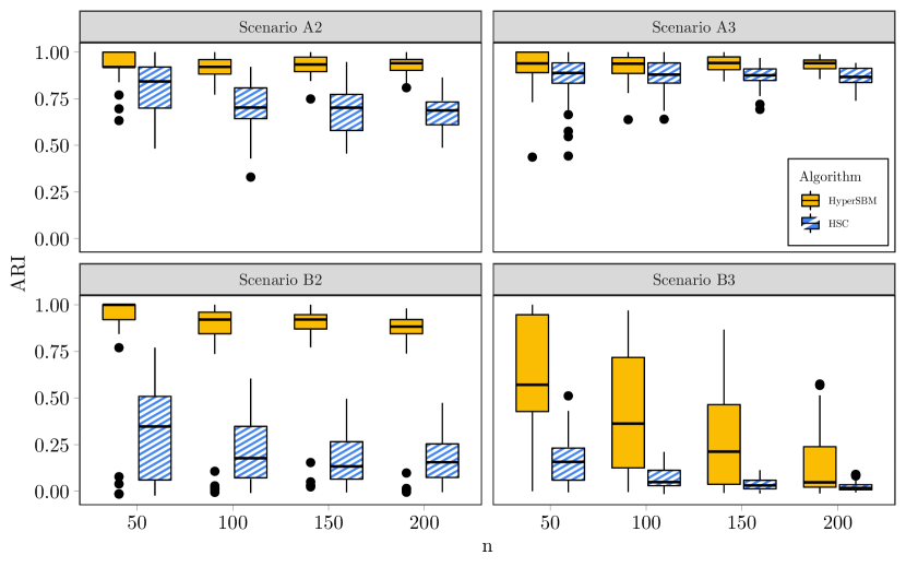
Figure 1: Boxplots of Adjusted Rand Indexes for different settings X$Q$ (where X=A, B is the scenario and $Q=2,3$ is the number of groups), number of nodes $n$ (along $x$-axis) and 2 methods: our HyperSBM (left boxplot) and HSC (right boxplot). First row (resp. first column) shows scenario A with communities (resp. $Q=2$) while second row (resp. second column) shows scenario B with disassortative behaviour (resp. $Q=3$).

Figure 1 displays the boxplot values of the ARI for settings A2 to B3. It is evident that our HyperSBM consistently outperforms HSC, obtaining higher ARI values overall and significantly lower variances in most cases, except for setting B3, where HyperSBM exhibits a larger variance but still yields substantially better results compared to HSC. We also observe that increasing the number of nodes $n$ does not appear to significantly enhance the clustering results of HyperSBM. This behavior could be attributed to our simulation setting, where the numbers of size-$m$ hyperedges ($m=2,3$) are kept linearly increasing with $n$. However, it is worth noting that the variances of the ARI obtained by HyperSBM tend to decrease with an increasing number of nodes $n$. One final comment pertains to the relatively poor clustering performance obtained by both methods in setting B3. This setting appears to be particularly challenging, indicating the necessity for further research on detectability thresholds in the context of non-uniform hypergraphs. We briefly discuss this topic in the next paragraph.

Detectability thresholds.

A threshold for community detection in $m$-uniform sparse hypergraphs is conjectured in Angelini et al. (2015) and Stephan and Zhu (2022) established it is efficiently achieved by a spectral algorithm based on the non-backtracking operator. We also mention the work by Zhang and Tan (2023) in a different regime. In the specific case of a symmetric $m$-uniform HSBM (which corresponds to (Aff) submodel) with equal group proportions (see Example 1 in Stephan and Zhu, 2022), the Kesten-Stigum (KS) threshold for possible recovery in the sparse regime is

$$KS_{m}=\frac{(m-1)(\alpha-\beta)^{2}}{Q^{m-1}(\alpha+(Q^{m-1}-1)\beta)}>1.$$

When the groups proportions are not uniform, we conjecture that this threshold becomes

$$\widetilde{KS}_{m}=\frac{(m-1)(\sum_{q}\pi_{q}^{m})^{2}(\alpha-\beta)^{2}}{(\sum_{q}\pi_{q}^{m})\alpha+(1-\sum_{q}\pi_{q}^{m})\beta}>1.$$

It appears that none of the 5 settings explored satisfies the $KS_{m}$ nor $\widetilde{KS}_{m}$ thresholds when restricting attention to either $m=2$ or $m=3$ (see Section E.3 in SM). Thus, in theory, the clusters cannot be recovered in those scenarios by looking only at $2$-uniforms or $3$-uniforms hypergraphs. Our results seem to indicate that non-uniform sparse hypergraphs behave differently than the superposition of their uniform layers and that the existence of hyperedges of different sizes improves the detectability of the clusters.

Parameter estimation accuracy.

We also evaluate the accuracy of parameter estimation. As the parameter values may be extremely small (see Section E in SM), we choose to compute the Mean Squared Relative Error (MSRE) between the true parameters (in the full model) and the estimated values, both for the prior probabilities $\pi_{q}$ and the probabilities of hyperedge occurrence $B^{(m)}_{q_{1},\ldots,q_{m}}$. Specifically, we compute the aggregated MSRE over all the components of $\theta$ using the following formula:

$$MSRE=\frac{1}{n_{rep}}\sum_{i=1}^{n_{rep}}\Big{\{}\sum_{q=1}^{Q-1}\Big{(}\frac{\hat{\pi}_{q}^{i}-\pi_{q}}{\pi_{q}}\Big{)}^{2}+\sum_{m=2}^{M}\sum_{q_{1}\leq\dots\leq q_{m}}\Big{(}\frac{\hat{B}_{q_{1},\dots,q_{m}}^{(m,n),i}-B^{(m,n)}_{q_{1},\dots,q_{m}}}{B^{(m,n)}_{q_{1},\dots,q_{m}}}\Big{)}^{2}\Big{\}},$$

where $(\hat{\pi}_{1}^{i},\dots,\hat{\pi}_{Q-1}^{i},\{\hat{B}_{q_{1},\dots,q_{m}}^{(m,n),i}\}_{m,q_{1},\dots,q_{m}})$ is the set of free parameters estimated on the $i$-th dataset by the full model and $n_{rep}=50$ is the number of replicates.

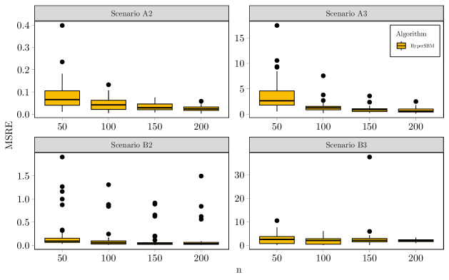
Figure 2: Boxplots of Mean Squared Relative Errors between true and estimated model parameters for different settings X$Q$ (where X=A, B is the scenario and $Q=2,3$ is the number of groups) and number of nodes $n$ (along $x$-axis). First row (resp. first column) shows scenario A with communities (resp. $Q=2$) while second row (resp. second column) shows scenario B with disassortative behaviour (resp. $Q=3$).

The corresponding results are summarized through the boxplots in Figure 2. The relative errors are rather small, decreasing and showing a lower variance as the number of nodes increases. Note that the absolute values of MSRE cannot be compared between the cases $Q=2$ (first column) and $Q=3$ (second column). Indeed, in the first case, the relative error is cumulated over a total of 1+3 +4=8 free parameters (in the full model), while this increases to 2+ 6+10=18 free parameters when $Q=3$.

3.3 Performance of model selection

In this section we assess the performance of ICL as a model selection criterion. The simulated data is fitted with our HyperSBM with a number of latent states ranging from 1 to 5.

$Q$	$n=50$	$n=100$	$n=150$	$n=200$
1	$0\%$	$0\%$	$0\%$	$0\%$
2	$26\%$	$2\%$	$0\%$	$0\%$
3	$74\%$	$98\%$	$100\%$	$100\%$
4	$0\%$	$0\%$	$0\%$	$0\%$
5	$0\%$	$0\%$	$0\%$	$0\%$

Table 2: Frequency (as a percentage) of the selected number of groups $Q$ for setting A3’. Model selection is carried out by means of the ICL criterion. Results are computed over 50 samples for each value of $n$.

In Table 2 we show the frequency of the selected number of groups for setting A3’. The correct model is selected in $74\%$ of cases for $n=50$, in $98\%$ of cases for $n=100$ and in $100\%$ of cases for $n=150,200$. We also compute the value of ARI of the classification obtained with 3 clusters depending on the selected number of latent groups. This value is always equal to 1 when the correct model is recovered, thus confirming the optimal behavior of HyperSBM already shown in Section 3.2.

3.4 Line clustering through hypergraphs

Following Leordeanu and Sminchisescu (2012); Kamiński et al. (2019) and earlier references, we here explore the use of hypergraphs to detect line clusters of points in $\mathbb{R}^{2}$. Similarly to the construction of pairwise similarity measures, we here resort on third order affinity measures to detect alignment of points since pairwise measures would be useless to detect alignment. Thus, for any triplet of points $\{i,j,k\}$, we use the mean distance to the best fitting line as a dissimilarity measure $d(i,j,k)$ and transform this through a Gaussian kernel to a similarity measure.

We performed two different experiments, with either 2 or 3 lines. In each setting, we randomly generate the same number of points per line in the range $[-0.5,0.5]^{2}$ and perturbed with centered Gaussian noise with standard deviation $0.01$. We then add noisy points, generated from uniform distribution on $[-0.5,0.5]^{2}$. The particular settings of each experiment are described in Table 3 and Figure 3 shows the resulting sets of points.

	Number of points per line	Number of noisy points	Total number of points	Mean number of hyperedges
2 lines	30	40	100	1070.84
3 lines	30	60	150	587.70

Table 3: Description settings for the line clustering experiments.

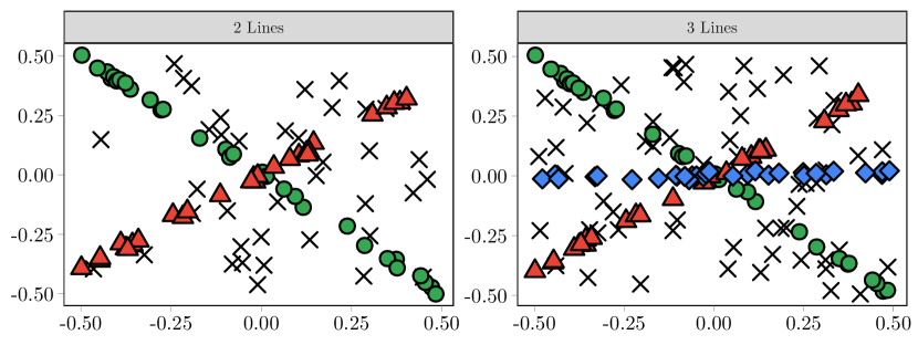
Figure 3: Sets of points from the line clustering experiments. Left: 2 lines (green dots and red triangles) plus noise (black crosses). Right: 3 lines (green dots, red triangles and blue diamonds) plus noise (black crosses).

For both settings, we generated 100 different 3-uniform hypergraphs using the following procedure. We randomly selected 3 points $\{i,j,k\}$ and calculated the mean distance $d(i,j,k)$ to the best-fitting line. We then measured their similarity using a Gaussian kernel $\exp(-d(i,j,k)^{2}/\sigma^{2})$ with $\sigma^{2}=0.04$. If the similarity was greater than a threshold $\epsilon=0.999$, we constructed a hyperedge $\{i,j,k\}$. This procedure resulted in both signal hyperedges, where all points belonged to the same line cluster, and noise hyperedges, where the points were sufficiently aligned without belonging to the same line. The signal-to-noise ratio of hyperedges was set to 2 for each hypergraph. We specifically simulated sparse hypergraphs, and the average number of hyperedges is presented in Table 3. Additionally, isolated nodes in the hypergraph were excluded from the clustering analysis.

We applied our HyperSBM algorithm to cluster the nodes of these 3-uniform and sparse hypergraphs, and we compared the results with three different modularity-based approaches. The first two approaches, referred to as Chodrow_Symm and Chodrow_AON, are from Chodrow et al. (2021) and are based on their general symmetric and all-or-nothing modularity, respectively. The third approach, referred to as Kaminski, is from Kamiński et al. (2019). The modularity-based methods automatically select the number of groups, and for HyperSBM, we performed model selection using $Q\in\{1,\dots,6\}$.

Figure 4 displays the ARI obtained from the clustering results. We can observe that the modularity-based methods fail to accurately recover the true original line clusters, resulting in lower ARIs. In contrast, HyperSBM shows good performance in this task, achieving higher ARIs. This difference in performance can be attributed to the tendency of modularity-based methods, especially the one by Kamiński et al. (2019), to select a larger number of groups in this particular context, as evidenced in Figure 5.

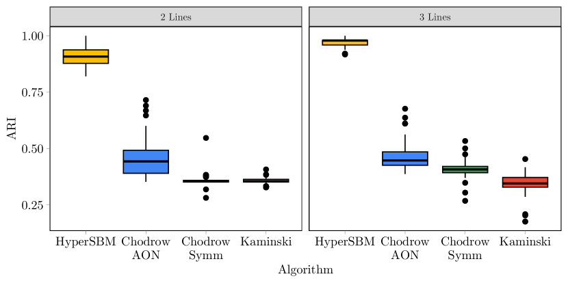
Figure 4: Boxplots of the ARI obtained by the different clustering methods on the line clustering problem. Left: 2 lines, right: 3 lines.

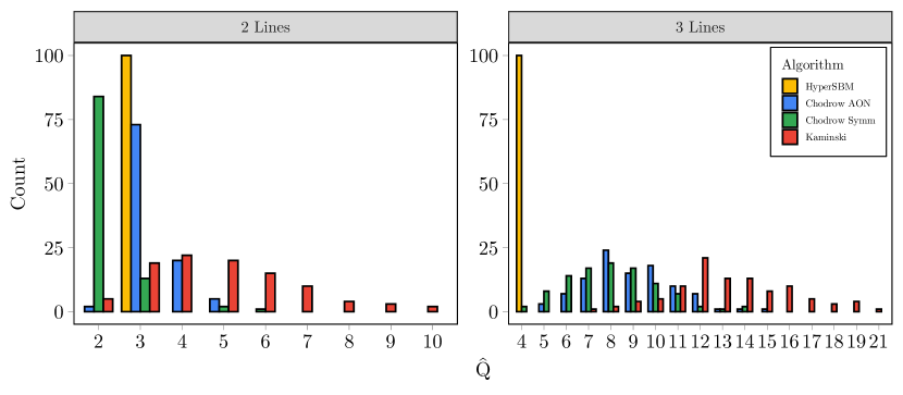
Figure 5: Estimated number of groups $\hat{Q}$ on the line clustering problem. Left: 2 lines (true value of $Q$ is 3), right: 3 lines (true value of $Q$ is 4).

This experiment highlights the distinct behavior of HyperSBM compared to the modularity-based clustering methods, including the approach proposed by Chodrow et al. (2021), despite both methods being based on a Stochastic Block Model (SBM) framework with a maximum-likelihood approach.

4 Analysis of a co-authorship dataset

4.1 Dataset description

We analyze a co-authorship dataset available at http://vlado.fmf.uni-lj.si/pub/networks/data/2mode/Sandi/Sandi.htm. The dataset originates from the bibliography of the book “Product Graphs: Structure and recognition” by Imrich and Klavzăr and is provided as a bipartite author/article graph. To construct the hypergraph, following the approach of Estrada and Rodríguez-Velázquez (2006), we consider authors as nodes and create hyperedges that link authors who have collaborated on the same paper. Further details regarding the dataset pre-treatment can be found in Section F of the SM, along with additional analyses. In our analysis, we set $M=4$ and focused on the main connected component of the hypergraph, which consists of 79 authors and 76 hyperedges. Among these hyperedges, 68.5% have a size of 2, while 29% have a size of 3, and 2.5% have a size of 4.

4.2 Analysis with HyperSBM

We conducted an analysis of this dataset using our HyperSBM package. The model selection based on the ICL criterion determined that there are 2 groups ($\hat{Q}=2$). One group consists of only 8 authors, while the remaining 71 authors belong to the second group. Table 4 displays the distribution of the number of distinct co-authors per author. Within the first group of 8 authors, 6 of them have the highest number of distinct co-authors, while the remaining 2 authors each have 4 distinct co-authors.

Nb co-authors	1	2	3	4	5	6	7	8	10	11	12
Count	23	27	13	6	2	2	1	1	2	1	1

Table 4: Distribution of the number of distinct co-authors per author. The first group contains the 6 authors having the largest number of distinct co-authors (between 7 and 12) plus 2 authors with 4 co-authors each.

Coming back to the bipartite graph of authors and (co-authored) papers, we looked at the degree distribution of the authors, given in Table 5. This corresponds to the distribution of the number of co-authored papers per author. We observed that 5 of the 8 authors from our first group are the ones that co-published the most, the three others having also high degree (one of degree 5 and two of degree 4). Thus, our first group is made of authors (among) the most collaborative ones, which are also (among) the most prolific ones.

Author degree	1	2	3	4	5	6	7	8	10	13
Count	44	14	6	6	4	1	1	1	1	1

Table 5: Degree distribution of authors in the bipartite graph. Our first group contains the 5 most collaborating authors, one of the sixth, plus 2 authors with degree equal to 4.

Neither the first nor the second group inferred by HyperSBM are communities. Indeed we obtained the following estimated values from the size-$2$ hyperedges: $\hat{B}^{(2)}_{11}\simeq 4.2\%$ is of the same order as $\hat{B}^{(2)}_{12}\simeq 5.1\%$ while $\hat{B}^{(2)}_{22}\simeq 0.8\%$ is around five times smaller. (We have dropped from our notation $\hat{B}^{(m,n)}$ the index $n$ and only use the size $m$ of the hyperedges to distinguish the parameter values). This means that the first group contains authors that have written with authors from the two groups while the second group is made of authors who have less co-authored papers with people of their own group. Looking now at size-3 hyperedges, we get that $\hat{B}^{(3)}_{111}\simeq 2\cdot 10^{-4}$ ; $\hat{B}^{(3)}_{112}\simeq 18\cdot 10^{-4}$ ; $\hat{B}^{(3)}_{122}\simeq 7\cdot 10^{-4}$ and $\hat{B}^{(3)}_{222}\simeq 0.6\cdot 10^{-4}$. The most important estimated frequency is $\hat{B}^{(3)}_{112}$ that concerns 2 authors of the small first group co-authoring a paper with one author of the large second group. The second most important estimated frequency is $\hat{B}^{(3)}_{122}$ and is obtained for one author from small first group co-authoring a paper with two authors of the large second group. The remaining frequencies of size-$3$ hyperedges are negligible. This characterizes further the first groups as being composed by authors that do co-author with their own group as well as with authors from the second one.

Finally, looking now at size-4 hyperedges, the only non negligible estimated frequency is obtained for $\hat{B}^{(4)}_{1222}\simeq 4\cdot 10^{-6}$. We note here that the quantities $B^{(3)}$’s and $B^{(4)}$’s are intrinsically on different scales, as are the quantities $B^{(2)}$’s and $B^{(3)}$’s. So again, authors from group one co-authored with the others authors. (Note that the first group is not large enough for a $B^{(4)}$ frequency with at least 2 authors in that group 1 to be non negligible).

4.3 Comparison with 2 other methods

We first compared our approach with the hypergraph spectral clustering (HSC) algorithm proposed in Ghoshdastidar and Dukkipati (2017). Let us recall that spectral clustering does not come with a statistical criterion to select the number of groups. Looking at the partition obtained with $Q=2$ groups, spectral clustering output groups with sizes 24 and 55, respectively. These groups are neither characterized by the number of co-authors nor their degrees in the bipartite graph (see details in SM). Indeed, in our case the best clusters are not communities and their sizes are very different, while we recall that spectral clustering tends to: i) extract communities ; ii) favor groups of similar size.

We then analysed the same dataset as a bipartite graph of authors/papers with the R package SBM through the function estimateBipartiteSBM (Chiquet et al., 2022). This method infers a latent blockmodel (that in fact corresponds to a SBM for bipartite graphs) and automatically selects a number of groups on both parts (authors and papers). Hereafter, we refer to this method as the Bipartite-SBM implementation. Let us underline here that while the bipartite stochastic blockmodel can be written as a particular case of a HSBM, the converse is not true (see Section A.3 in the SM).

The Bipartite-SBM also selected 2 groups of authors (and one group of papers). There was one small group with 4 authors, entirely contained in our first small group; it corresponds to authors that have the highest degree in the bipartite graph and the highest number of co-authors. So, Bipartite-SBM output a very small group of the most prolific and the most collaborative authors in this dataset. Further details about the distinctions between these groups and the ones obtained by HyperSBM are given in SM.

As a conclusion, we see that while the outputs of Bipartite-SBM and HyperSBM may seem close on this specific dataset, they are nonetheless different. On the other hand, and still on this specific dataset, the spectral clustering approach outputs results that are completely different from those of HyperSBM.

5 Proofs

Proof of Lemma 1.

We consider a fixed value of $m\geq 2$ and denote by $\llbracket a,b\rrbracket$ the set of integer values between $a,b$. Let us recall that $B^{(m,n)}$ is a fully symmetric tensor (1), so the number of free parameters in $B^{(m,n)}$ is equal to the number of ordered sequences $q_{1}\leq\dots\leq q_{m}$ of elements in $\llbracket 1,Q\rrbracket$. We denote by $\mathcal{Q}^{+}$ this set. Then we define a function $f$ which, to any such sequence $\underline{q}=(q_{1},\dots,q_{m})$, associates the value $\underline{l}=f(\underline{q})$ defined by $f(\underline{q})=(q_{1},q_{2}+1,q_{3}+2,\dots,q_{m}+m-1)$. We let $\mathcal{L}^{+}$ denote the set of sequences $\underline{l}=(l_{1},\dots,l_{m})$ with coordinates in $\llbracket 1,Q+m-1\rrbracket$ and such that $l_{1}<l_{2}<\dots<l_{m}$. Thus, for any $\underline{q}\in\mathcal{Q}^{+}$ we get that $f(\underline{q})\in\mathcal{L}^{+}$.

Conversely, for any $\underline{l}=(l_{1},\dots,l_{m})\in\mathcal{L}^{+}$, we can associate the value $\underline{q}=g(\underline{l})=(l_{1},l_{2}-1,l_{3}-2,\dots,l_{m}-m+1)$. It is easy to see that the image $\underline{q}=g(\underline{l})$ belongs to $\mathcal{Q}^{+}$.

As a consequence, the functions $f$ and $g$ are such that their composition is the identity function: $f\circ g=g\circ f=Id$. These are one-to-one functions mapping $\mathcal{Q}^{+}$ to $\mathcal{L}^{+}$ and conversely. This implies that the cardinalities of these two sets are equal. But an element in $\mathcal{L}^{+}$ is exactly a subset of size $m$ of $\llbracket 1,Q+m-1\rrbracket$ so that the cardinality of $\mathcal{L}^{+}$ is the number of subsets of size $m$ of $\llbracket 1,Q+m-1\rrbracket$. This concludes the proof of the lemma. ∎

Proof of Theorem 2.

The proof closely follows the structure of the proof for Theorem 2 in Allman et al. (2011) for the SBM on simple graphs, with the generalization to simple $m$-uniform HSBM. The complete details of this generalization can be found in Section C of the SM. In this section, we focus on the key element that distinguishes our proof from the proof of Theorem 2 in Allman et al. (2011). This crucial element involves constructing a set of degree sequences with specific properties. Due to the fundamental differences in characterizing which integer sequences can be realized as degree sequences between graphs and $m$-uniform hypergraphs, our construction differs from the one presented in the proof of Theorem 2 in Allman et al. (2011).

Consider the following set of integer-valued sequences

$$\mathcal{D}=\Big{\{}\mathbf{d}=(d_{1},\ldots,d_{n_{0}})~{}|~{}\text{ for }1\leq i\leq n_{0},d_{i}\in\{m,2m,3m,\ldots,Qm\}\Big{\}}.$$

Lemma 7.

The set $\mathcal{D}$ of $n_{0}$-length integer sequences satisfies

• for each $i\in\{1,\ldots,n_{0}\}$, the set of $i$-th coordinates $\{d_{i}~{}|~{}\mathbf{d}\in\mathcal{D}\}$ has cardinality at most $Q$;

• For large enough $n_{0}$ (depending on $Q,m$), any $\mathbf{d}\in\mathcal{D}$ is the degree sequence of a simple $m$-uniform hypergraph over $n_{0}$ nodes;

• $|\mathcal{D}|\geq Q^{n_{0}}$.

Note that conditions $(i),(iii)$ imply that $\{d_{i}~{}|~{}\mathbf{d}\in\mathcal{D}\}$ should have cardinality exactly $Q$ and that $|\mathcal{D}|=Q^{n_{0}}$.

Proof of Lemma 7.

Points $(i),(iii)$ are a consequence of the definition of $\mathcal{D}$. For any integer sequence $\mathbf{d}$, a necessary condition for $\mathbf{d}$ to be a degree sequence of a simple $m$-uniform hypergraph over $n_{0}$ nodes is that $m$ divides $\sum_{i}d_{i}$. Here, we rather need sufficient conditions in order to prove $(ii)$. We rely on Corollary 2.2 in Behrens et al. (2013).

Corollary 2.2 in Behrens et al. (2013).

Let $\mathbf{d}$ be an integer-valued sequence with maximum term $\Delta$ and let $p$ be an integer such that $\Delta\leq\binom{p-1}{m-1}$. If $m$ divides $\sum_{i}d_{i}$ and $\sum_{i}d_{i}\geq(\Delta-1)p+1$ then $\mathbf{d}$ is the degree sequence of a simple $m$-uniform hypergraph.

Fix some $\mathbf{d}\in\mathcal{D}$. Note that by construction, $m$ divides $\sum_{i}d_{i}$. Let $\Delta$ be the maximum value of this sequence and note that $\Delta\leq Qm$. Thus we choose $p$ an integer such that $Qm\leq\binom{p-1}{m-1}$. Moreover, $\sum_{i}d_{i}\geq mn_{0}$ and $(\Delta-1)p+1\leq\Delta p\leq Qmp$. Then by choosing $n_{0}\geq Qp$, we obtain the desired result. ∎

With Lemma 7 at hand, we are able to generalize the proof of Theorem 2 in Allman et al. (2011) for simple graphs SBM to the case of simple $m$-uniform HSBM. This concludes the proof of Theorem 2. ∎

Proof of Corollary 3.

From the probability distribution $\mathbb{P}_{\theta}$ over simple hypergraphs $\mathcal{H}$ on a set of $n$ nodes and hyperedges with largest size $M$, we automatically obtain all the probability distributions $\mathbb{P}_{\theta}$ restricted to simple $m$-uniform hypergraphs $\mathcal{H}_{m}$ on the same set of nodes. Applying the result of Theorem 2 for all values $m$ is sufficient to obtain the desired result. Indeed, as $M$ is finite, the union of the finite number of lower-dimensional subspaces where identifiability for fixed $m$ may not be satisfied gives a lower-dimensional subspace, ensuring generic identifiability. Moreover, for each value of $m$, we recover the parameter $\theta^{(m)}$ up to a permutation on $\{1,\dots,Q\}$. Now, for any $m\neq m^{\prime}$ it remains to be able to jointly order the parameters $\theta^{(m)}$ and $\theta^{(m^{\prime})}$ up to a permutation on $\{1,\dots,Q\}$. If all the $\pi_{q}$’s are different, which is a generic condition, this can be easily done because $\theta^{(m)}$ and $\theta^{(m^{\prime})}$ share the same distinct $\pi_{q}$’s. ∎

Proof of Proposition 4.

We want to maximize $\mathcal{J}({\theta},{\tau})$ with respect to $\tau_{iq}$ under the constraint $\sum_{q=1}^{Q}\tau_{iq}=1$ for all $i$. Using the method of Lagrange multipliers, this is equivalent to maximizing with respect to $\tau_{iq}$ the Lagrangian function

$$\Lambda({\theta},{\tau},{\lambda}) =\sum_{i=1}^{n}\lambda_{i}\Bigg{(}\sum_{q=1}^{Q}\tau_{iq}-1\Bigg{)}+\mathcal{J}({\theta},{\tau})$$

$$=\sum_{i=1}^{n}\lambda_{i}\Bigg{(}\sum_{q=1}^{Q}\tau_{iq}-1\Bigg{)}+\sum_{q=1}^{Q}\sum_{i=1}^{n}\tau_{iq}\log\frac{\pi_{q}}{\tau_{iq}}$$

$$\phantom{=}+\sum_{i=1}^{n}\sum_{q=1}^{Q}\sum_{m=1}^{M-1}\sum_{q_{1}\leq\dots\leq q_{m}}\sum_{\mathcal{V}^{(m)}\not\ni i}\tau_{iq}\tau_{i_{1}q_{1}}\cdots\tau_{i_{m}q_{m}}f(Y_{ii_{1}\dots i_{m}},B^{(m+1,n)}_{qq_{1}\dots q_{m}})$$

Computing the partial derivative of $\Lambda(\theta,\bm{\tau},\bm{\lambda})$ with respect to $\tau_{iq}$, we obtain the following expression

$$\frac{\partial\Lambda}{\partial\tau_{iq}} =\lambda_{i}+\log\frac{\pi_{q}}{\tau_{iq}}-1$$

$$\phantom{=}+\sum_{m=1}^{M-1}\sum_{q_{1}\leq\dots\leq q_{m}}\sum_{\mathcal{V}^{m}\not\ni i}\tau_{i_{1}q_{1}}\cdots\tau_{i_{m}q_{m}}f(Y_{ii_{1}\dots i_{m}},B^{(m+1,n)}_{qq_{1}\dots q_{m}})$$

$$=\lambda_{i}+\log\pi_{q}-\log\tau_{iq}-1$$

$$\phantom{=}+\log\prod_{m=1}^{M-1}\prod_{q_{1}\leq\dots\leq q_{m}}\prod_{\mathcal{V}^{m}\not\ni i}\left[\exp(f(Y_{ii_{1}\dots i_{m}},B^{(m+1,n)}_{qq_{1}\dots q_{m}}))\right]^{\tau_{i_{1}q_{1}}\cdots\tau_{i_{m}q_{m}}},$$

which is equal to 0 if

$$\tau_{iq}=e^{\lambda_{i}-1}\ \pi_{q}\prod_{m=1}^{M-1}\prod_{q_{1}\leq\dots\leq q_{m}}\prod_{\mathcal{V}^{m}\not\ni i}\left[(\exp(f(Y_{ii_{1}\dots i_{m}},B^{(m+1,n)}_{qq_{1}\dots q_{m}}))\right]^{\tau_{i_{1}q_{1}}\cdots\tau_{i_{m}q_{m}}}.$$

The term $e^{\lambda_{i}-1}=\frac{1}{\sum_{q=1}^{Q}\tau_{iq}}$ is the normalizing constant such that $\sum_{q=1}^{Q}\tau_{iq}=1$ for each $i$.
Finally, let us remark that the Lagrangian function $\Lambda$ is concave with respect to each $\tau_{iq}$, being the sum of a concave term ($\tau_{iq}\log(\pi_{q}/\tau_{iq})$) and linear terms. Then the critical point is a maximum. ∎

Proof of Proposition 5.

For the prior probabilities $\pi_{q}$, we want to maximize $\mathcal{J}({\theta},{\tau})$ with respect to $\pi_{q}$ subject to the constraint $\sum_{q=1}^{Q}\pi_{q}=1$. Using again Lagrange multipliers, this is equivalent to maximizing

$$\Lambda({\theta},{\tau},{\lambda})=\lambda\Bigg{(}\sum_{q=1}^{Q}\pi_{q}-1\Bigg{)}+\mathcal{J}({\theta},{\tau})$$

Noting that the second term of $\mathcal{J}({\theta},{\tau})$ does not depend on $\pi_{q}$, the computation of the partial derivative of $\Lambda({\theta},{\tau},{\lambda})$ reduces to

$$\frac{\partial}{\partial\pi_{q}}\Bigg{[}\lambda\bigg{(}\sum_{q=1}^{Q}\pi_{q}-1\bigg{)}+\sum_{q=1}^{Q}\sum_{i=1}^{n}\tau_{iq}\log\frac{\pi_{q}}{\tau_{iq}}\Bigg{]}=\lambda+\sum_{i=1}^{n}\frac{\tau_{iq}}{\pi_{q}}.$$

This quantity is equal to 0 if

$$\pi_{q}=-\frac{1}{\lambda}\sum_{i=1}^{n}\tau_{iq},$$

where $\lambda=-n$ is the normalizing constant in order to satisfy $\sum_{q=1}^{Q}\pi_{q}=1$.
Note the Lagrangian function $\Lambda$ is concave with respect to each $\pi_{q}$, being the sum of a concave term ($\log(\pi_{q}/\tau_{iq})$), of a linear term ($\lambda\sum_{q=1}^{Q}\pi_{q}$) and of a constant. The critical point is then a maximum.

Finally, the partial derivative w.r.t. $B^{(m,n)}_{q_{1},\dots,q_{m}}$ is

$$\frac{\partial\mathcal{J}}{\partial B^{(m,n)}_{q_{1},\dots,q_{m}}}=\sum_{\mathcal{V}^{m}}\tau_{i_{1}q_{1}}\cdots\tau_{i_{m}q_{m}}\left[Y_{i_{1}\dots i_{m}}\frac{1}{B^{(m,n)}_{q_{1}\dots q_{m}}}-(1-Y_{i_{1}\dots i_{m}})\frac{1}{1-B^{(m,n)}_{q_{1}\dots q_{m}}}\right].$$

Through some basic algebraic manipulations, this quantity results equal to 0 if

$$B^{(m,n)}_{q_{1},\dots,q_{m}}=\frac{\sum_{\mathcal{V}^{m}}\tau_{i_{1}q_{1}}\cdots\tau_{i_{m}q_{m}}Y_{i_{1}\dots i_{m}}}{\sum_{\mathcal{V}^{m}}\tau_{i_{1}q_{1}}\cdots\tau_{i_{m}q_{m}}}.$$

Again, the Lagrangian function is the sum of a concave term ($\log B^{(m,n)}_{q_{1},\dots,q_{m}}$) and of some constant terms, thus being a concave function. The critical point is then a maximum. ∎

Proof of Proposition 6.

The following decomposition of $\mathcal{J}(\theta,\tau)$ naturally holds:

$$\mathcal{J}(\theta,\tau) =\sum_{q=1}^{Q}\sum_{i=1}^{n}\tau_{iq}\log\frac{\pi_{q}}{\tau_{iq}}$$

$$\phantom{=}+\sum_{m=2}^{M}\sum_{q=1}^{Q}\sum_{\mathcal{V}^{m}}\tau_{i_{1}q}\cdots\tau_{i_{m}q}\left[Y_{i_{1},\dots,i_{m}}\log\alpha^{(m,n)}+(1-Y_{i_{1},\dots,i_{m}})\log(1-\alpha^{(m,n)})\right]$$

$$\phantom{=}+\sum_{m=2}^{M}\sum_{\begin{subarray}{c}q_{1}\leq\dots\leq q_{m}\\ |\{q_{1},\dots,q_{m}\}|\geq 2\end{subarray}}\sum_{\mathcal{V}^{m}}\tau_{i_{1}q_{1}}\cdots\tau_{i_{m}q_{m}}\left[Y_{i_{1},\dots,i_{m}}\log\beta^{(m,n)}+(1-Y_{i_{1},\dots,i_{m}})\log(1-\beta^{(m,n)})\right].$$

The partial derivative w.r.t. $\alpha^{(m,n)}$ is

$$\frac{\partial\mathcal{J}}{\partial\alpha^{(m,n)}}=\sum_{q=1}^{Q}\sum_{\mathcal{V}^{m}}\tau_{i_{1}q}\cdots\tau_{i_{m}q}\left[Y_{i_{1}\dots i_{m}}\frac{1}{\alpha^{(m,n)}}-(1-Y_{i_{1}\dots i_{m}})\frac{1}{1-\alpha^{(m,n)}}\right],$$

hence it follows that:

$$\widehat{\alpha}^{(m,n)}=\frac{\sum_{q=1}^{Q}\sum_{\{i_{1},\dots,i_{m}\}\in\mathcal{V}^{m}}\tau_{i_{1}q}\dots\tau_{i_{m}q}Y_{i_{1}\dots i_{m}}}{\sum_{q=1}^{Q}\sum_{\{i_{1},\dots,i_{m}\}\in\mathcal{V}^{m}}\tau_{i_{1}q}\dots\tau_{i_{m}q}}.$$

Analogously, the partial derivative w.r.t. $\beta^{(m,n)}$ is

$$\frac{\partial\mathcal{J}}{\partial\beta^{(m,n)}}=\sum_{\begin{subarray}{c}q_{1}\leq\dots\leq q_{m}\\ |\{q_{1},\dots,q_{m}\}|\geq 2\end{subarray}}\sum_{\mathcal{V}^{m}}\tau_{i_{1}q_{1}}\cdots\tau_{i_{m}q_{m}}\left[Y_{i_{1}\dots i_{m}}\frac{1}{\beta^{(m,n)}}-(1-Y_{i_{1}\dots i_{m}})\frac{1}{1-\beta^{(m,n)}}\right],$$

and

$$\widehat{\beta}^{(m,n)}=\frac{\sum_{\begin{subarray}{c}q_{1}\leq\dots\leq q_{m}\\ |\{q_{1},\dots,q_{m}\}|\geq 2\end{subarray}}\sum_{\{i_{1},\dots,i_{m}\}\in\mathcal{V}^{m}}\tau_{i_{1}q_{1}}\dots\tau_{i_{m}q_{m}}Y_{i_{1}\dots i_{m}}}{\sum_{\begin{subarray}{c}q_{1}\leq\dots\leq q_{m}\\ |\{q_{1},\dots,q_{m}\}|\geq 2\end{subarray}}\sum_{\{i_{1},\dots,i_{m}\}\in\mathcal{V}^{m}}\tau_{i_{1}q_{1}}\dots\tau_{i_{m}q_{m}}}.$$

This concludes the proof for the formulas under assumption (Aff-m). The expressions for $\hat{\alpha}^{(n)}$ and $\hat{\beta}^{(n)}$ under assumption (Aff) are computed in the same way. ∎

6 Codes availability

The algorithm implementation in C++ is available as an R package called HyperSBM at https://github.com/LB1304/HyperSBM. The Supplementary Material, the files to reproduce the synthetic experiments and the dataset analysis are available at
https://github.com/LB1304/Hypergraph-Stochastic-Blockmodel.

Supplementary Material to: Model-based clustering in simple hypergraphs through a stochastic blockmodel
By Luca Brusa & Catherine Matias

All non-alphabetic references are concerned with the main text.

Appendix A Limits of the bipartite graphs representation of hypergraphs

A.1 Bipartite graphs and multiple hypergraphs with self-loops equivalence

Some early analyses of hypergraphs rely on the embedding of the former into the space of bipartite graphs (see for e.g. Battiston et al., 2020). Indeed, any hypergraph $\mathcal{H}=(\mathcal{V},\mathcal{E})$ where $\mathcal{V}$ is the set of nodes and $\mathcal{E}$ the set of hyperedges may be represented as a bipartite graph with two parts. The top part is simply the set $\mathcal{V}$ of hypergraph nodes, while the bottom part is the set $\mathcal{E}$ of hyperedges and there is a link between $v\in\mathcal{V}$ and $e\in\mathcal{E}$ whenever node $v$ belongs to hyperedge $e$ in the original hypergraph $\mathcal{H}$.

Now, it is possible to define a “converse” application from bipartite graphs to hypergraphs. Indeed, any bipartite graph can be projected into two distinct hypergraphs, by choosing one of the two parts as the nodes set and forming a hyperedge with any set of nodes that are neighbors (in the bipartite graph) of the same node (belonging to the second part). A major difference appears whether we consider simple hypergraphs or multiple hypergraphs with self-loops. In multiple hypergraphs  (not to be confused with multiset hypergraphs) hyperedges may appear several time so that these are weighted hypergraphs with integer valued weights. We also allow for self-loops, i.e hyperedges of cardinality 1. Then, this application from bipartite graphs to hypergraphs slightly differs depending on whether we allow the image of a bipartite graph to be a multiple hypergraphs with self-loops or a simple hypergraph. In the first case, all the information from the bipartite graph will be encoded in the multiple hypergraphs with self-loops; while in the second case, part of the information will be lost. This is illustrated on a toy example in Figure 6.

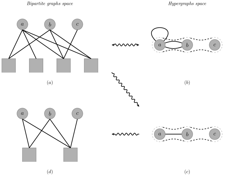
Figure 6: (a) A bipartite graph $\mathcal{G}$; (b) Projection of $\mathcal{G}$ into the multiple hypergraphs with self-loops space, choosing the top nodes as the new set of nodes. Hyperedges are $\{a\},\{a,b\},\{a,b\},\{a,b,c\}$. The applications from (a) to (b) are invertible bijections, one being the inverse of the other; (c) Projection of $\mathcal{G}$ on the simple hypergraphs subspace. Hyperedges are $\{a,b\},\{a,b,c\}$. (d) Embedding of the simple hypergraph in (c) in the bipartite graphs space. Note that (a) and (d) are not the same bipartite graph.

The embedding of the simple hypergraphs space into the bipartite graphs space is not the inverse of the natural projection of bipartite graphs into simple hypergraphs. Thus, models of bipartite graphs are inappropriate to handle simple hypergraphs, as the former generally put mass on any bipartite graph, notwithstanding the fact that not all of these may be realized as the image of a simple hypergraph. For the same reason, preferential attachment models of bipartite graphs (Guillaume and Latapy, 2004) may not be directly used for simple hypergraphs as they would produce unconstrained bipartite graphs that do not necessarily come from simple hypergraphs.

A.2 Artefacts induced by bipartite graphs models

In order to view a bipartite graph as a hypergraph, one first needs to select the top and bottom parts. Swapping the role of the two parts will in general give another hypergraph. Statistical models of bipartite graphs handle the two parts symmetrically and do not differentiate between a top and a bottom part. They are thus inadequate for modeling hypergraphs.

One may also note that most random bipartite graphs models are designed for fixed parts sizes, which induces, on top of a fixed number of nodes, a fixed number of hyperedges in the corresponding hypergraph model, an artifact which is not always desirable. For instance the uniformly random hypergraphs model allows for any possible density on the hyperedges.

A last example of inadequacy is given by configuration models on bipartite graphs that induce configuration models on hypergraphs. In these models, the degree distributions in each part are kept fixed. When projected in the hypergraphs space, that means that the degrees of the nodes and the sizes of the hyperedges are kept fixed. Then, relying on shuffling algorithms to explore the space of this configuration model, one will loose the labels on the bottom part (the hyperedges part) as these are automatically induced by the new edges of the bipartite graph and the labelling of the top part (the nodes part). As a consequence, if a specific node tends to take part in large size hyperedges, this information is lost in the configuration model issued from bipartite graphs.

To our knowledge, there is no configuration model on hypergraphs that only keeps the nodes degrees sequence fixed. We mention that Section 4 from Chodrow (2020) provides a discussion about the limitations of the embedding approach in terms of the types of hypergraph null models from which we can conveniently sample. In particular, Chodrow (2020) establishes that there is no obvious route for vertex-label sampling in hypergraphs through bipartite random graphs.

A.3 HSBM is not a bipartite SBM

In this section, we briefly outline that (i) while the bipartite stochastic blockmodel can be seen as a particular case of HSBM, (ii) the converse is not true in general.

To see point (i), let us consider a bipartite SBM on a graph $\mathcal{G}$ with nodes divided in 2 parts, say $\mathcal{V}=\{1,\dots,n\}$ and $\mathcal{U}=\{1,\dots,e\}$. The model has $Q$ groups (resp. $R$ groups) on the subset of nodes $\mathcal{V}$ (resp. $\mathcal{U}$), with group proportions $\pi$ (resp. $\eta$). We let $Z_{1},\dots,Z_{n}$ (resp. $W_{1},\dots,W_{e}$) denote the latent groups of nodes $\mathcal{V}$ (resp. $\mathcal{U}$).

The model is also given by a connectivity matrix $M$ of size $Q\times R$ whose entries $M_{qr}$ are the conditional probabilities that a node in $\mathcal{V}$ from group $q$ connects a node in $\mathcal{U}$ from group $r$. In other words $M_{qr}=\mathbb{P}(X_{iu}=1|Z_{i}=q,W_{u}=r)$ where $X=(X_{iu})$ is the $n\times e$ incidence matrix of $\mathcal{G}$.

Now consider the hypergraph $\mathcal{H}$ constructed on the set of nodes $\mathcal{V}$ and whose hyperedges are obtained by looking at the set of nodes in $\mathcal{V}$ connected to a same node in $\mathcal{U}$. (A similar construction could be made with swapping the roles of $\mathcal{V}$ and $\mathcal{U}$). Then, the probability distribution of $\mathcal{H}$ under the induced bipartite SBM is exactly a HSBM with $Q$ groups, with group proportions $\pi$ and parameters

$$B^{(m,n)}_{q_{1},\dots,q_{m}} =\mathbb{P}(Y_{i_{1},\dots,i_{m}}=1|Z_{i_{1}}=q_{1},\dots,Z_{i_{m}}=q_{m})$$

$$=\mathbb{P}(X_{i_{1},u}=1,\dots,X_{i_{m},u}=1|Z_{i_{1}}=q_{1},\dots,Z_{i_{m}}=q_{m})$$

$$=\sum_{r=1}^{R}\mathbb{P}(X_{i_{1},u}=1,\dots,X_{i_{m},u}=1,W_{u}=r|Z_{i_{1}}=q_{1},\dots,Z_{i_{m}}=q_{m})$$

$$=\sum_{r=1}^{R}\eta_{r}\prod_{q=q_{1}}^{q_{m}}M_{qr},$$

where $u$ is the node that connects $\{i_{1},\dots,i_{m}\}$ into a hyperedge. So we see that the bibartite SBM induces a HSBM with constrained connection probabilities.

Let us now explain why (ii) the converse is not true in general. We start from a HSBM with $Q$ groups and parameters $(\pi,(B^{(m,n)}_{q_{1},\dots,q_{m}})_{q_{1},\dots,q_{m}})_{2\leq m\leq M}$ on a hypergraph $\mathcal{H}$ with set of nodes $\mathcal{V}$. Considering $\mathcal{U}=\{1,\dots,e\}$ where $e$ is the number of hyperedges in $\mathcal{H}$, we construct a bipartite graph $\mathcal{G}$ with nodes $\mathcal{V}\times\mathcal{U}$ and links between any $i\in\mathcal{V}$ and any $u\in\mathcal{U}$ whenever node $i$ belongs to hyperedge $u$ in the hypergraph $\mathcal{H}$. Now, if there is a bipartite SBM on $\mathcal{G}$ with same distribution as our HSBM, then necessarily it has $Q$ groups on $\mathcal{V}$, with group proportions given by $\pi$. We let $R$ denote the number of groups on such a model on $\mathcal{U}$, together with $\eta$ the corresponding group proportions, and $M$ the $Q\times R$ matrix of connection probabilities. Then we observe that $\eta$ and $M$ should satisfy the relations:

$$\forall 2\leq m\leq M,\forall q_{1},\dots,q_{m}\in\{1,\dots,Q\}^{m},\quad B^{(m,n)}_{q_{1},\dots,q_{m}}=\sum_{r=1}^{R}\eta_{r}\prod_{q=q_{1}}^{q_{m}}M_{qr}.$$ (10)

Here, we first remark that the bipartite SBM fit on the co-authorship dataset (from Section 4) selected $R=1$, thus inducing hyperedges connectivity parameters with a product form

$$B^{(m,n)}_{q_{1},\dots,q_{m}}=\prod_{q=q_{1}}^{q_{m}}M_{q1}.$$

Our fitted HSBM on this same dataset did not result in hyperedges connectivity parameters with a product form, which establishes that the models are clearly different.

Now, more generally, we could ask whether for given parameters $(B^{(m,n)}_{q_{1},\dots,q_{m}})_{2\leq m\leq M}$, there exist some values of $R,\eta$ and $M$ such that (10) is satisfied. The answer is: not always. To see this, consider for instance $Q=2$ and remark the relation between the two quantities

$$B^{(2,n)}_{11} =\sum_{r=1}^{R}\eta_{r}M_{1r}^{2},$$

$$B^{(3,n)}_{111} =\sum_{r=1}^{R}\eta_{r}M_{1r}^{3},$$

so that $B^{(2,n)}_{11}$ and $B^{(3,n)}_{111}$ cannot be chosen independently.

Appendix B The need for simple hypergraphs models

In this section, we discuss modeling differences between multiset hypergraphs where multiset hyperedges are allowed, versus simple hypergraphs where hyperedges are subsets of nodes. We recall that multiset hypergraphs allow for repeated nodes in a same hyperedge, the latter being defined as a multiset of nodes. Multiset hyperedges generalize in some sense the notion of self-loops in graphs and thus are a natural extension to consider. However, they are not appropriate in all contexts. For instance, a co-authorship dataset cannot contain hyperedges with repeated nodes (but may contain a self-loop of a unique author). In the same way, a social interaction hypergraph does not contain multisets hyperedges; triadic interactions are restricted to 3 different individuals and self-loops are not allowed. In the meantime, they are natural in other contexts; consider, e.g., chemical reaction hypergraphs where the multiplicity plays the role of the stoichiometric coefficients (Flamm et al., 2015). We first argue that multisets-hypergraph models are inappropriate for analysing simple hypergraphs.

B.1 A motivating example

Let us first focus on parameter estimates rather than on clustering. For the sake of simplicity, we restrict our attention to $3$-uniform hypergraphs on a set of $n$ nodes and consider two different models. The first one, denoted as MH, acts on $3$-uniform multiset hypergraphs and draws a hyperedge between any 3 nodes, not necessarily distinct, with probability $p_{\text{MH}}$. The second one, denoted as SH, acts on $3$-uniform simple hypergraphs and draws a hyperedge between any 3 distinct nodes with probability $p_{\text{SH}}$.

Now, we consider a toy example of observing a simple hypergraph $\mathcal{H}$ with $n=3$ nodes and only one hyperedge $e=\{1,2,3\}$. This dataset could correspond to observing for instance one publication with 3 authors. When analysed under the MH model, the density of our observed hypergraph is estimated by

$$\hat{p}_{\text{MH}}=1/27$$

because there are $n^{3}=27$ possible size-$3$ multiset hyperedges under this model, and just one of these is observed. On the contrary, when analysed under the SH model, we infer a density of

$$\hat{p}_{\text{SH}}=1$$

because the only possible size-$3$ hyperedge is observed. As a consequence, the statistical conclusions drawn on this dataset will highly differ depending on whether we restrict attention to simple hypergraphs or work with more general multiset hypergraphs. This choice of the ambient space has to be made according to the specificities of the dataset. This simple and elementary example shows that it is not possible to statistically analyse a simple hypergraph with a multiset hypergraphs model without erroneous conclusions.

B.2 Null model for multiset hypergraphs in modularity computations

The main technical difference between multiset hypergraphs and simple hypergraphs analysis comes from the enumeration of size-$m$ subsets of nodes. In the multiset hypergraphs setting, the summations over multisets of nodes $\{i_{1},\dots,i_{m}\}\in\{1,\dots,n\}^{m}$ factorize into $m$ independent sums. On the contrary, in the simple hypergraph setting, the summations involve sets of nodes $\{i_{1},\dots,i_{m}\}$ that are constrained to be distinct. As a consequence, such a factorization is impossible.

Let us consider a concrete example. We already emphasized the fact that modularity criteria for hypergraphs have been proposed only in the multiset hypergraphs setting (Kamiński et al., 2019; Chodrow et al., 2021). Modularities are generally constructed as deviation measures of the number of hyperedges from their expected number under a null model. For instance in the graphs context, the Newman and Girvan modularity of a partition $(C_{1},\dots,C_{Q})$ of the nodes into $Q$ clusters is computed as

$$\text{Modularity}(C_{1},\dots,C_{Q}) =\frac{1}{2|E|}\sum_{q=1}^{Q}\sum_{i,j\in C_{q}}\Big{(}A_{ij}-\frac{d_{i}d_{j}}{2|E|}\Big{)}$$

$$=\frac{1}{2|E|}\sum_{q=1}^{Q}\sum_{i,j\in C_{q}}A_{ij}-\frac{1}{2|E|}\sum_{q=1}^{Q}\sum_{i,j\in C_{q}}\frac{d_{i}d_{j}}{2|E|},$$

where $A=(A_{ij})_{i,j}$ is the graph adjacency matrix, $d_{i}$ is the degree of node $i$, and $2|E|=\sum_{i}d_{i}$ is twice the number of edges. While the first part of these criteria enumerates only the occurring hyperedges, a quantity that is small in general as most hypergraph datasets are sparse, the second part needs to account for all subset of nodes in the graph (or at least in the same group $C_{q}$). In the case of graphs allowing self-loops, this second term factorizes to

$$\frac{1}{2|E|}\sum_{q=1}^{Q}\sum_{i,j\in C_{q}}\frac{d_{i}d_{j}}{2|E|}=\frac{1}{2|E|}\sum_{q=1}^{Q}\frac{(\sum_{i\in C_{q}}d_{i})(\sum_{j\in C_{q}}d_{j})}{2|E|}=\sum_{q=1}^{Q}\frac{\text{Vol}(q)^{2}}{(2|E|)^{2}},$$

where the computation of the volume $\text{Vol}(q)=\sum_{i\in C_{q}}d_{i}$ has time complexity of $O(n)$. Similarly, for multiset hypergraphs the modularity computed in Chodrow et al. (2021) uses two main terms: the first is a cut term that depends only on occurring hyperegdes while the second relies on volumes of latent configurations of the nodes (see Eq. (12) and (13) in Chodrow et al., 2021). On the contrary, in the simple hypergraph setting, enumerating all subsets of nodes constrained to be distinct requires enumerating

$$\sum_{m=2}^{M}\binom{n}{m}$$

elements for a hypergraph with $n$ nodes and maximum hyperedge size $M$. This quantity is huge and represents the main computational limit when analysing hypergraphs (our approach to this issue is detailed in Section D from SM).

Appendix C The complete proof of Theorem 2

For the sake of completeness, we provide here the complete proof of Theorem 2. This proof mostly reproduces the proof of Theorem 2 in Allman et al. (2011).

The strategy relying on Kruskal’s result.

The proof strongly relies on an algebraic result from Kruskal (1977) that appeared to be a powerful tool to establish identifiability results in various models whose common feature is the presence of discrete latent groups and at least three conditionally independent random variables. We first rephrase Kruskal’s result in a statistical context. Consider a latent random variable $V$ with state space $\{1,\ldots,r\}$ and distribution given by the column vector $\mathbf{v}=(v_{1},\ldots,v_{r})$. Assume that there are three observable random variables $U_{j}$ for $j=1,2,3$, each with finite state space $\{1,\ldots,\kappa_{j}\}$. The $U_{j}$s are moreover assumed to be independent conditional on $V$. Let $M_{j}$, $j=1,2,3$ be the stochastic matrix of size $r\times\kappa_{j}$ whose $i$th row is $\mathbf{m}_{i}^{j}=\mathbb{P}(U_{j}=\cdot\mid V=i)$. Then consider the $3$-dimensional array (or tensor) with dimensions $\kappa_{1}\times\kappa_{2}\times\kappa_{3}$ denoted $[\mathbf{v};M_{1},M_{2},M_{3}]$ and whose $(s,t,u)$ entry (for any $1\leq s\leq\kappa_{1},1\leq t\leq\kappa_{2},1\leq u\leq\kappa_{3}$) is defined by

$$[\mathbf{v};M_{1},M_{2},M_{3}]_{s,t,u} =\sum_{i=1}^{r}v_{i}m^{1}_{i}(s)\,m^{2}_{i}(t)\,m^{3}_{i}(u)$$

$$=\sum_{i=1}^{r}\mathbb{P}(V=i)\mathbb{P}(U_{1}=s|V=i)\mathbb{P}(U_{2}=t|V=i)\mathbb{P}(U_{3}=u|V=i)$$

$$=\mathbb{P}(U_{1}=s,U_{2}=t,U_{3}=u).$$

Note that $[\mathbf{v};M_{1},M_{2},M_{3}]$ is left unchanged by simultaneously permuting the rows of all the $M_{j}$ and the entries of $\mathbf{v}$, as this corresponds to permuting the labels of the latent classes. Knowledge of the distribution of $(U_{1},U_{2},U_{3})$ is equivalent to knowledge of the tensor $[\mathbf{v};M_{1},M_{2},M_{3}]$.
Now, the Kruskal rank of a matrix $M$, denoted $\operatorname{rank}_{K}M$, is the largest number $I$ such that every set of $I$ rows of $M$ are independent. Note that for any matrix $M$, its Kruskal rank is necessarily less than its rank, namely $\operatorname{rank}_{K}M\leq\operatorname{rank}M$, and equality of rank and Kruskal rank does not hold in general. However, in the particular case when a matrix $M$ of size $p\times q$ has rank $p$, it also has Kruskal rank $p$. Now, let $I_{j}=\operatorname{rank}_{K}M_{j}$. Kruskal (1977) established the following result. If

$$I_{1}+I_{2}+I_{3}\geq 2r+2,$$ (11)

then the tensor $[\mathbf{v};M_{1},M_{2},M_{3}]$ uniquely determines $\mathbf{v}$ and the $M_{j}$, up to simultaneous permutation of the rows. In other words, the set of parameters $\{(\mathbf{v},\mathbb{P}(U_{j}=\cdot\mid V))\}$ is uniquely identified, up to label switching on the latent groups, from the distribution of the random variables $(U_{1},U_{2},U_{3})$.

Now, to obtain generic identifiability, it is sufficient to exhibit a single parameter value for which (11) is satisfied. Indeed, the set of parameter values for which $\operatorname{rank}_{K}M_{j}$ is fixed can be expressed through a Boolean combination of polynomial inequalities ($\neq$, or rather non-equalities) involving matrix minors in those parameters. In the same way, the converse condition of (11), namely inequality $I_{1}+I_{2}+I_{3}\leq 2r+1$ is the finite Boolean combination of polynomial non-equalities on the model parameters. This means that this set of parameters is an algebraic variety. But an algebraic variety can only be either the whole parameter space (in which case exhibiting a single value where (11) is satisfied would not be possible) or a proper subvariety, thus a subspace of dimension strictly lower than that of the whole parameter space.

The strategy of the proof for showing identifiability of certain discrete latent class models developed in Allman et al. (2011) and other papers by the same authors is to embed these models in the context of Kruskal’s result just described. Applying Kruskal’s result to the embedded model, the authors derive partial identifiability results on the embedded model, and then, using details of the embedding, relate these to the original model.

Embedding the HSBM into Kruskal’s setup.

For some number of nodes $n$ (to be specified later), we let $V=(Z_{1},Z_{2},\dots,Z_{n})$ be the latent random variable, with state space $\{1,\ldots,Q\}^{n}$ and denote by $\mathbf{v}$ the corresponding vector of its probability distribution. The entries of $\mathbf{v}$ are of the form $\pi_{1}^{n_{1}}\cdots\pi_{Q}^{n_{Q}}$ for some integers $n_{q}\geq 0$ and such that $\sum_{q}n_{q}=n$. We fix $m\geq 2$ and consider simple $m$-uniform hypergraphs on the set of nodes $\mathcal{V}=\{1,\dots,n\}$. Recall that $\mathcal{V}^{(m)}$ is the set of all distinct $m$-tuples of nodes in $\mathcal{V}$ and $\{Y_{i_{1},\dots,i_{m}};\{i_{1},\dots,i_{m}\}\in\mathcal{V}^{(m)}\}$ the set of all indicator variables corresponding to possible (simple) hyperedges of a $m$-uniform hypergraph over $\mathcal{V}$. Now, we will construct below subsets $H_{1},H_{2},H_{3}\subset\mathcal{V}^{(m)}$ of distinct $m$-tuples of nodes such that $H_{i}\cap H_{j}=\emptyset$ for any $i\neq j$. Then, we choose the 3 observed variables $U_{j}$ ($1\leq j\leq 3$) as the vectors of indicator variables $U_{j}=(Y_{i_{1},\dots,i_{m}})_{\{i_{1},\dots,i_{m}\}\in H_{j}}$. This induces that $\kappa_{j}=2^{|H_{j}|}$ (where $|H_{j}|$ is the cardinality of $H_{j}$). As the subsets $H_{1},H_{2},H_{3}$ do not share any $m$-tuple of nodes, the random variables $U_{j}$ are conditionally independent given $V$. We are in the statistical context of Kruskal’s result.

The goal is now to construct the 3 subsets $H_{j}$ of $m$-tuples such that their pairwise intersections are empty and such that condition (11) is satisfied (for at least one parameter value of the embedded model and thus generically for this embedded model). This construction of the $H_{j}$’s proceeds in two steps: the base case and an extension step.

Starting with a small set $\mathcal{V}_{0}=\{1,\dots,n_{0}\}$ of nodes, we define a matrix $A$ of dimension $Q^{n_{0}}\times 2^{\binom{n_{0}}{m}}$. Its rows are indexed by latent configurations $v\in\{1,\ldots,Q\}^{n_{0}}$ of the nodes in $\mathcal{V}_{0}$, its columns by the set of all possible states of the vector of indicator variables $(Y_{i_{1},\dots,i_{m}})_{\{i_{1},\dots,i_{m}\}\in\mathcal{V}_{0}}$, and the entries of $A$ give the probability of observing the specified states of the vector of indicator variables, conditioned on the latent configurations $v$. Thus each column index corresponds to a different simple $m$-uniform hypergraph on $\mathcal{V}_{0}$. The base case consists in exhibiting a value of ${n_{0}}$ such that this matrix $A$ generically has full row rank. Then, in an extension step, relying on $n=n_{0}^{2}$ nodes, we construct the subsets $H_{1},H_{2},H_{3}$ with the desired properties (namely their pairwise intersections are empty and (11) is generically satisfied).

From Kruskal’s theorem, we obtain that the vector $\mathbf{v}$ and the matrices $M_{1},M_{2},M_{3}$ are generically uniquely determined, up to simultaneous permutation of the rows from the distribution of a simple $m$-uniform HSBM.

With these embedded parameters $\mathbf{v},M_{1},M_{2},M_{3}$ in hand, it is still necessary to recover the initial parameters of the simple $m$-uniform HSBM: the group proportions $\pi_{q}$ and the connectivity matrix $B^{(m)}=(B^{(m,n)}_{q_{1},\dots,q_{m}})_{1\leq q_{1}\leq\dots\leq q_{m}\leq Q}$. This will be done in the conclusion.

Base case.

In the following, we drop the exponents $(m,n)$ in the notation for the connection probabilities $B$ and simply let $B_{q_{1},\dots,q_{m}}=\mathbb{P}(Y_{i_{1},\dots,i_{m}}=1\mid Z_{i_{1}}=q_{1},\dots,Z_{i_{m}}=q_{m})=1-\bar{B}_{q_{1},\dots,q_{m}}$. The initial step consists in finding a value of ${n_{0}}$ such that the matrix $A$ of size $Q^{n_{0}}\times 2^{\binom{n_{0}}{m}}$ containing the probabilities of any simple $m$-uniform hypergraph over these ${n_{0}}$ nodes, conditional on the hidden node states, generically has full row rank.

The condition of having full row rank can be expressed as the non-vanishing of at least one $Q^{n_{0}}\times Q^{n_{0}}$ minor of $A$. Composing the map sending the parameters $\{B_{q_{1},\dots,q_{m}}\}\to A$ with this collection of minors gives polynomials in the parameters of the model. To see that these polynomials are not identically zero, and thus are non-zero for generic parameters, it is enough to exhibit a single choice of the $\{B_{q_{1},\dots,q_{m}}\}$ for which the corresponding matrix $A$ has full row rank. We choose to consider parameters $\{B_{q_{1},\dots,q_{m}}\}$ of the form

$$B_{q_{1},\dots,q_{m}}=\frac{s_{q_{1}}s_{q_{2}}\dots s_{q_{m}}}{s_{q_{1}}s_{q_{2}}\dots s_{q_{m}}+t_{q_{1}}t_{q_{2}}\dots t_{q_{m}}},\text{ so }\bar{B}_{q_{1},\dots,q_{m}}=\frac{t_{q_{1}}t_{q_{2}}\dots t_{q_{m}}}{s_{q_{1}}s_{q_{2}}\dots s_{q_{m}}+t_{q_{1}}t_{q_{2}}\dots t_{q_{m}}},$$

with $s_{q},t_{l}>0$ to be chosen later. However, since the property of having full row rank is unchanged under non-zero rescaling of the rows of the matrix $A$, and all entries of $A$ are monomials with total degree $\binom{n_{0}}{m}$ in $B_{q_{1},\dots,q_{m}},\bar{B}_{q_{1},\dots,q_{m}}\}$, we may simplify the entries of $A$ by removing denominators, and consider the matrix (also called $A$) with entries in terms of $B_{q_{1},\dots,q_{m}}=s_{q_{1}}s_{q_{2}}\dots s_{q_{m}}$ and $\bar{B}_{q_{1},\dots,q_{m}}=t_{q_{1}}t_{q_{2}}\dots t_{q_{m}}$.

The rows of $A$ are indexed by the composite node states $v\in\{1,\ldots,Q\}^{n_{0}}$, while its columns are indexed by the $m$-uniform hypergraphs $\mathcal{H}=(y_{i_{1},\dots,i_{m}})_{\{i_{1},\dots,i_{m}\}\in\mathcal{V}_{0}}\in\{0,1\}^{\binom{n_{0}}{m}}$. For any composite hidden state $v\in\{1,\ldots,Q\}^{n_{0}}$ and any node $i\in\{1,\ldots,{n_{0}}\}$, let $v(i)\in\{1,\ldots,Q\}$ denote the state of node $i$ in the composite state $v$. With our particular choice of the parameters $B_{q_{1},\dots,q_{m}}$, the $(v,\mathcal{H})$-entry of $A$ is given by

$$\prod_{\{i_{1}\dots i_{m}\}\in\mathcal{V}_{0}^{(m)}}B_{v(i_{1}),\dots,v(i_{m})}^{y_{i_{1},\dots,i_{m}}}\bar{B}_{v(i_{1}),\dots,v(i_{m})}^{1-y_{i_{1},\dots,i_{m}}}=\prod_{i=1}^{n_{0}}s_{v(i)}^{d_{i}}t_{v(i)}^{{n_{0}}-1-d_{i}},$$

where

$$d_{i}=\sum_{\begin{subarray}{c}\{i_{1}\dots i_{m}\}\in\mathcal{V}_{0}^{(m)}\\ i\in\{i_{1}\dots i_{m}\}\end{subarray}}y_{i_{1},\dots,i_{m}}$$

is the degree of node $i$ in the hypergraph $\mathcal{H}=(y_{i_{1},\dots,i_{m}})_{\{i_{1},\dots,i_{m}\}\in\mathcal{V}_{0}}$. With this choice of parameters $\{B_{q_{1},\dots,q_{m}}\}$, the entries in a column of $A$ are entirely determined by the degree sequence $\mathbf{d}=(d_{i})_{1\leq i\leq{n_{0}}}$ of the hypergraph under consideration. Two different hypergraphs may result in the same degree sequence, thus the same values in the two columns of $A$. For any degree sequence $\mathbf{d}=(d_{i})_{1\leq i\leq{n_{0}}}$ arising from a simple $m$-uniform hypergraph on $n_{0}$ nodes, let $A_{\mathbf{d}}$ denote a corresponding column of $A$. In order to prove that the matrix $A$ has full row rank, it is enough to exhibit $Q^{n_{0}}$ independent columns of $A$. To this aim, we introduce polynomial functions whose independence is equivalent to that of corresponding columns.

For each node $i\in\{1,\ldots,{n_{0}}\}$ and each latent group $q\in\{1,\ldots,Q\}$, introduce an indeterminate $X_{i,q}$ and a $Q^{n_{0}}$-size row vector $\mathbf{X}=(\prod_{1\leq i\leq{n_{0}}}X_{i,v(i)})_{v\in\{1,\ldots,Q\}^{n_{0}}}$. For each degree sequence $\mathbf{d}$, we have

$$\mathbf{X}A_{\mathbf{d}}=\sum_{v\in\{1,\ldots,Q\}^{n_{0}}}\prod_{1\leq i\leq{n_{0}}}s_{v(i)}^{d_{i}}t_{v(i)}^{{n_{0}}-1-d_{i}}X_{i,v(i)}=\prod_{1\leq i\leq{n_{0}}}\left(s_{1}^{d_{i}}t_{1}^{{n_{0}}-1-d_{i}}X_{i,1}+\cdots+s_{Q}^{d_{i}}t_{Q}^{{n_{0}}-1-d_{i}}X_{i,Q}\right).$$

Now, independence of a set of columns $\{A_{\mathbf{d}}\}$ is equivalent to the independence of the corresponding set of polynomial functions $\{\mathbf{X}A_{\mathbf{d}}\}$ in the indeterminates $\{X_{i,q}\}$. For a set $\mathcal{D}$ of degree sequences, to prove that the polynomials $\{\mathbf{X}A_{\mathbf{d}}\}_{\mathbf{d}\in\mathcal{D}}$ are independent, we assume that there exist scalars $a_{\mathbf{d}}$ such that

$$\sum_{\mathbf{d}\in\mathcal{D}}a_{\mathbf{d}}\mathbf{X}A_{\mathbf{d}}\equiv 0,$$ (12)

and show that necessarily all $a_{\mathbf{d}}=0$. This will be given by the following lemma from Allman et al. (2011). This lemma is originally formulated for a set $\mathcal{D}$ of degree sequences. However it is not specific to degree sequences; it applies for any sets $\mathcal{D}$ of sequences of integers indexed by $\{1,\dots,n_{0}\}$ and thus we phrase it in this way. We refer to Allman et al. (2011) for its proof.

Lemma 8.

(Lemma 18 in Allman et al. (2011).) Assume $n_{0}\geq Q$. Let $\mathcal{D}$ be a set of $n_{0}$-length integer sequences such that for each $i\in\{1,\ldots,n_{0}\}$, the set of $i$-th coordinates $\{d_{i}~{}|~{}\mathbf{d}\in\mathcal{D}\}$ has cardinality at most $Q$. Then for generic values of $s_{q},t_{l}$, for each $i$ and each $d^{\star}\in\{d_{i}~{}|~{}\mathbf{d}\in\mathcal{D}\}$ there exist values of the indeterminates $\{X_{i,q}\}_{1\leq q\leq Q}$ that annihilate all the polynomials $\mathbf{X}A_{\mathbf{d}}$ for $\mathbf{d}\in\mathcal{D}$ except those for which $d_{i}=d^{\star}$.

The next step is to construct a set $\mathcal{D}$ of $n_{0}$-length integer sequences that satisfies

• for each $i\in\{1,\ldots,n_{0}\}$, the set of $i$-th coordinates $\{d_{i}~{}|~{}\mathbf{d}\in\mathcal{D}\}$ has cardinality at most $Q$ (condition in Lemma 8);

• any $\mathbf{d}\in\mathcal{D}$ may be the degree sequence of a simple $m$-uniform hypergraph;

• $|\mathcal{D}|\geq Q^{n_{0}}$.

With such a set at hand, by choosing one column of $A$ associated to each degree sequence in $\mathcal{D}$, we obtain a collection of $|\mathcal{D}|\geq Q^{n_{0}}$ different columns of $A$. These columns are independent since for each sequence $\mathbf{d}^{\star}\in\mathcal{D}$, by Lemma 8 we can choose values of the indeterminates $\{X_{i,q}\}_{1\leq i\leq n_{0},1\leq q\leq Q}$ such that all polynomials $\mathbf{X}A_{\mathbf{d}}$ vanish, except $\mathbf{X}A_{\mathbf{d}^{\star}}$, leading to $a_{\mathbf{d}^{\star}}=0$ in equation (12). Thus, exhibiting such a set $\mathcal{D}$ is the last step to prove that $A$ has generically full row rank.

Now, this is where our proof strongly differs from the one of Theorem 2 in Allman et al. (2011). Indeed, the characterizations of degree sequences for graphs and simple $m$-uniform hypergraphs are completely different. Relying on a result by Behrens et al. (2013), we have exhibited such a set in Lemma 7.

This concludes the proof of the base case.

The extension step.

The extension step builds on the base case, in order to construct a larger set of $n=n_{0}^{2}$ nodes and subsets $H_{1},H_{2},H_{3}\subset\mathcal{V}^{(m)}$ of distinct $m$-tuples of nodes in $\mathcal{V}=\{1,\dots,n\}$ with the desired properties. This step was first stated as Lemma 16 in Allman et al. (2009) in the context of simple graphs SBM and we extend it below to our case.

Let us recall that we want to construct $H_{1},H_{2},H_{3}\subset\mathcal{V}^{(m)}$ that are pairwise disjoint. Then, with notation from above, we choose the 3 observed variables $U_{j}$ ($1\leq j\leq 3$) as the vectors of indicator variables $U_{j}=(Y_{i_{1},\dots,i_{m}})_{\{i_{1},\dots,i_{m}\}\in H_{j}}$. As the subsets $H_{1},H_{2},H_{3}$ do not share any $m$-tuple of nodes, the random variables $U_{j}$ are conditionally independent given $V=(Z_{1},\dots,Z_{n})$. We let $M_{j}$ denote the $Q^{n}\times 2^{|H_{j}|}$ matrix of conditional probabilities of $U_{j}$ given $Z$.

Lemma 9.

Suppose that for some number of nodes $n_{0}$, the matrix $A$ of size $Q^{n_{0}}\times 2^{\binom{n_{0}}{m}}$ defined above has generically full row rank. Then with $n=n_{0}^{2}$ there exist pairwise disjoint subsets $H_{1},H_{2},H_{3}\subset\mathcal{V}^{(m)}$ of $m$-tuples of nodes in $\mathcal{V}=\{1,\dots,n\}$ such that for each $j$ the $Q^{n}\times 2^{|H_{j}|}$ matrix $M_{j}$ has generically full row rank ($Q^{n}$).

Proof of Lemma 9.

Let us describe the construction of $H_{j}$. We will partition the $n_{0}^{2}$ nodes into $n_{0}$ groups of size $n_{0}$ in three different ways, each way leading to one $H_{j}$. Then each $H_{j}$ will be the union of the $n_{0}$ sets of all $m$-tuples made of some $n_{0}$ nodes. Thus each $H_{j}$ has cardinality $n_{0}\binom{n_{0}}{m}$.

Labeling the nodes by $(u,v)\in\{1,\cdots,n_{0}\}\times\{1,\cdots,n_{0}\}$, we picture the nodes as lattice points in a square grid. We take as the partition leading to $H_{1}$ the rows of the grid, as the partition leading to $H_{2}$ the columns of the grid, and as the partition leading to $H_{3}$ the diagonals. In other words, $H_{1}$ is the union over $n_{0}$ rows of all $m$-tuples of nodes within each row. The same with columns and diagonals. Explicitly, we define two functions $u,v$ that associate to any $i\in\{1,\dots,n_{0}\}$ its coordinates $(u(i),v(i))$ on the $n_{0}\times n_{0}$ grid. Then, the $H_{j}$ are $m$-tuple of nodes defined as

$$H_{1} =\cup_{u=1}^{n_{0}}H_{1}(u)=\cup_{u=1}^{n_{0}}\{\{i_{1},\dots,i_{m}\}\in\mathcal{V}^{(m)}~{}|~{}\forall k,u(i_{k})=u,v(i_{k})\in\{1,\cdots,n_{0}\}\},$$

$$H_{2} =\cup_{v=1}^{n_{0}}H_{2}(v)=\cup_{v=1}^{n_{0}}\{\{i_{1},\dots,i_{m}\}\in\mathcal{V}^{(m)}~{}|~{}\forall k,v(i_{k})=v,u(i_{k})\in\{1,\cdots,n_{0}\}\},$$

$$H_{3} =\cup_{s=1}^{n_{0}}H_{3}(s)$$

$$=\cup_{s=1}^{n_{0}}\{\{i_{1},\dots,i_{m}\}\in\mathcal{V}^{(m)}~{}|~{}\forall k,u(i_{k})=s,v(i_{k})=s+t\operatorname{mod}n_{0}\text{ for some }t\in\{1,\cdots,n_{0}\}\}.$$

The $H_{j}$ are pairwise disjoints as required.

The matrix $M_{j}$ of conditional probabilities of $U_{j}$ given $Z$ has $Q^{n}$ rows indexed by composite states of all $n=n_{0}^{2}$ nodes, and $2^{n_{0}\binom{n_{0}}{m}}$ columns indexed by $m$-tuples in $H_{j}$.

Observe that with an appropriate ordering of the rows and columns (which is dependent on $j$), $M_{j}$ has a block structure given by

$$M_{j}=A\otimes A\otimes\cdots\otimes A\text{ ($n_{0}$ factors)}.$$ (13)

(Note that since $A$ is $Q^{n_{0}}\times 2^{\binom{n_{0}}{m}}$, the tensor product on the right is $(Q^{n_{0}})^{n_{0}}\times\left(2^{\binom{n_{0}}{m}}\right)^{n_{0}}$ which is $Q^{n_{0}^{2}}\times 2^{n_{0}\binom{n_{0}}{m}}$, the size of $M_{j}$.) That $M_{j}$ is this tensor product is most easily seen by noting the partitioning of the $n_{0}^{2}$ nodes into $n_{0}$ disjoint sets (rows, columns and diagonals of the grid) gives rise to $n_{0}$ copies of the matrix $A$, one for each set of all simple $m$-uniform hypergraphs over $n_{0}$ nodes. The row indices of $M_{j}$ are obtained by choosing an assignment of states to the nodes in $H_{j}(u)$ for each $u$ independently, and the column indices by the union of independently-chosen simple $m$-uniform hypergraphs subgraphs on $H_{j}(u)$ for each $u$. This independence in both rows and columns leads to the tensor decomposition of $M_{j}$.

Now since $A$ has generically full row rank ($Q^{n_{0}}$), equation (13) implies that $M_{j}$ does as well (i.e has row rank $Q^{n_{0}^{2}}=Q^{n}$). ∎

Next, with $\mathbf{v},M_{1},M_{2},M_{3}$ defined by the embedding given in the previous paragraphs, we apply Kruskal’s Theorem to the table $[\mathbf{v};M_{1},M_{2},M_{3}]$. By construction of the $M_{j}$, condition (11) is generically satisfied since $3Q^{n}\geq 2Q^{n}+2$. Thus the vector $\mathbf{v}$ and the matrices $M_{1},M_{2},M_{3}$ are generically uniquely determined, up to simultaneous permutation of the rows from the distribution of a simple $m$-uniform HSBM.

It now remains to recover the original parameters of the simple $m$-uniform HSBM: the group proportions $\pi_{q}$ and the connectivity matrix $(B^{(m,n)}_{q_{1},\dots,q_{m}})_{1\leq q_{1}\leq q_{m}\leq Q}$.

Conclusion for the original model.

The entries of $\mathbf{v}$ are of the form $\pi_{1}^{n_{1}}\cdots\pi_{Q}^{n_{Q}}$ with $\sum n_{q}=n$, while the entries of the $M_{j}$ contain information on the $B^{(m,n)}_{q_{1},\dots,q_{m}}$. Although the ordering of the rows of the $M_{j}$ is arbitrary, crucially we do know how the rows of $M_{j}$ are paired with the entries of $\mathbf{v}$.

By focusing on one of the matrices, say $M_{1}$, and adding appropriate columns of it, we can obtain marginal conditional probabilities of single hyperedge variables, namely a column vector with values $(\mathbb{P}_{\theta}(Y_{i_{1},\dots,i_{m}}=1|(Z_{1},\dots,Z_{n})=v))_{v}$ for any $m$-tuple $\{i_{1},\dots,i_{m}\}$. Indeed, this vector is obtained by summing all the columns of $M_{1}$ corresponding to simple $m$-uniform hypergraphs with $Y_{i_{1},\dots,i_{m}}=1$. Thus, we recover the set of values $\{B^{(m,n)}_{q_{1},\dots,q_{m}}\}_{1\leq q_{1}\leq\dots\leq q_{m}\leq Q}$, but without order. Namely, we still do not know the $B^{(m,n)}_{q_{1},\dots,q_{m}}$ up to a permutation on $\{1,\dots,Q\}$ only, but rather up to a permutation on $\{1,\dots,Q\}^{n}$.

In the following, we assume without loss of generality, as it is a generic condition, that all $\{B^{(m,n)}_{q_{1},\dots,q_{m}}\}_{1\leq q_{1}\leq\dots\leq q_{m}\leq Q}$ are distinct.

We look at the first $(m+1)$ nodes $\mathcal{V}_{1}=\{1,\dots,m,m+1\}$ and consider the $m+1$ different $m$-tuples $\{i_{1},\dots,i_{m}\}\in\mathcal{V}_{1}^{(m)}$ that can be made from these nodes ($i_{k}\in\mathcal{V}_{1}$). Again, for each of these $m$-tuples, adding appropriate columns of $M_{1}$, we can jointly obtain the vectors of conditional marginal probabilities $(\mathbb{P}_{\theta}(Y_{\{i_{1},\dots,i_{m}\}}=1|(Z_{1},\dots,Z_{n})=v))_{v}$. Jointly means that all those vectors share the same ordering over the index $v\in\{1,\dots,Q\}^{n}$. In other words, we recover the sets of values

$$\forall v\in\{1,\dots,Q\}^{n},\quad R_{v}=\{B^{(m,n)}_{v_{i_{1}},\dots,v_{i_{m}}};\{i_{1},\dots,i_{m}\}\in\mathcal{V}_{1}^{(m)}\}.$$

Now, we assumed the $B$’s are all distinct so the cardinalities of the sets $R_{v}$ will help us discriminate the different parameters (up to a permutation on $\{1,\dots,Q\}$ only). Indeed, there are exactly $Q$ sets $R_{v}$ with cardinality exactly one. These corresponds to the cases were $v=(q,q,\dots,q)$ for some $1\leq q\leq Q$. From this, we can distinguish the parameters of the form $\{B^{(m,n)}_{q,\dots,q};1\leq q\leq Q\}$ from the complete set of parameters. Note that the corresponding entries of $v$ are given by $\pi_{q}^{m}$. So we also recover the paired values $\{(\pi_{q},B^{(m,n)}_{q,\dots,q});1\leq q\leq Q\}$. Then, we continue with the sets $R_{v}$ with cardinality two: these are of the form $\{B^{(m)}_{q,\dots,q};B^{(m,n)}_{q,\dots,q,l}\}$ for some $1\leq q\neq l\leq Q$. As we already identified the parameters $\{B^{(m,n)}_{q,\dots,q};1\leq q\leq Q\}$ and all $B$’s are distinct, this enables us to identify the set of parameters $\{B^{(m,n)}_{q,\dots,q,l};1\leq q\neq l\leq Q\}$. By induction, we recover the set of parameters $\{B^{(m,n)}_{q,\dots,q,l,l^{\prime}};1\leq q,l,l^{\prime}\leq Q\text{ and }q,l,l^{\prime}\text{ distinct}\}$ et caetera, ending with the set of parameters $\{B^{(m,n)}_{q_{1},\dots,q_{m}};1\leq q_{1}<q_{2}<\dots<q_{m}\leq Q\}$. This means that we finally have obtained the parameters $\{\pi_{q},B^{(m,n)}_{q_{1},\dots,q_{m}}\}_{1\leq q\leq Q;1\leq q_{1}\leq\dots\leq q_{m}\leq Q}$ up to a permutation over $\{1,\dots,Q\}$.

Finally, note that all generic aspects of this argument, in the base case and the requirement that the parameters $B^{(m,n)}_{q_{1},\dots,q_{m}}$ be distinct, concern only the $B^{(m,n)}_{q_{1},\dots,q_{m}}$. Thus if the group proportions $\pi_{q}$ are fixed to any specific values, the theorem remains valid.

Remark.

The requirement on large enough $n$ is more precisely given as $n\geq Q^{2}p^{2}$ where $p$ is the smallest integer such that $\binom{p-1}{m-1}\geq Qm$. A rough approximation gives that $p$ is of the order $(Qm)^{1/(m-1)}$ which gives that $n$ should be larger than $Q^{2}(Qm)^{2/(m-1)}$.

Appendix D Computational details on the algorithm’s implementation

In order to provide an efficient implementation, the whole estimation algorithm is implemented in C++ language using the Armadillo library for linear algebra. Moreover the implementation is made available in R by means of the R packages Rcpp (Eddelbuettel and François, 2011; Eddelbuettel, 2013) and RcppArmadillo (Eddelbuettel and Sanderson, 2014). In the following we consider some of the most relevant computational details.

Dealing with heavy computational cost.

Dealing with very large data structures, the main drawback of the proposed algorithm is the intensive computational effort, in terms of both execution time needed to converge and required memory space. The most outstanding example regards the computation of the products $\tau_{i_{1}q_{1}}\cdots\tau_{i_{m}q_{m}}$, required both in the VE-Step (see Proposition 4, for $\tau_{iq}$) and in the M-Step (see Proposition 5, for $B^{(m,n)}_{q_{1},\dots,q_{m}}$). The huge computational cost of this calculation derives from the large number of potential unordered node tuples even for rather small values of $n$ and $m$; indeed $|\mathcal{V}^{(m)}|=\binom{n}{m}$. A first possibility is to compute all the products $\tau_{i_{1}q_{1}}\cdots\tau_{i_{m}q_{m}}$ in a recursive manner at the beginning of each VEM iteration and to store them in a matrix. Although this is actually very beneficial for the computational time, the resulting matrix is huge, having number of rows and columns equal to $\binom{n}{m}$ and $\binom{Q+m-1}{m}$ respectively. The result is a structure that is intractable except for very small values of $n$, $Q$, and (especially) $m$. Taking into account that every element requires 8 bytes, we report some examples in Table 6, in order to better clarify the magnitude of the quantity to store. Stated the impossibility to store a matrix of such size, the computation of the required products $\tau_{i_{1}q_{1}}\cdots\tau_{i_{m}q_{m}}$ is implemented directly inside the VE- and M-Steps through nested loops; this process involves an important increase in the computing times, but on the other hand requires a minimal amount of memory. To handle the slowness of the computation, both the VE-Step and the M-Step are efficiently implemented in parallel through the RcppParallel package (Allaire et al., 2022).

$n$	$m$	$Q$	Memory size		$n$	$m$	$Q$	Memory size
100	3	2	$\approx 5.2\ MB$		500	3	2	$\approx 0.6\ GB$
100	3	4	$\approx 25.9\ MB$		500	3	4	$\approx 3.3\ GB$
100	6	2	$\approx 66.8\ GB$		500	6	2	$\approx 1179.2\ TB$
100	6	4	$\approx 801.1\ GB$		500	6	4	$\approx 14150.8\ TB$

Table 6: Memory size of the matrix containing the products $\tau_{i_{1}q_{1}}\cdots\tau_{i_{m}q_{m}}$ for given values of $n$ (number of nodes), $Q$ (number of latent groups) and $m$ (hyperedge size).

Floating point underflow.

Another crucial aspect is the possible occurrence of numerical instability deriving from the multiplication of many small values in the computation of $\widehat{\tau}_{iq}$. A simple remedy is provided by the calculation of $\log\widehat{\tau}_{iq}$ instead of $\widehat{\tau}_{iq}$. So, denoting $b_{iq}=\log(\hat{\tau}_{iq})-c_{i}$, we compute $\hat{\tau}_{iq}$ relying on

$$\widehat{\tau}_{iq}=\frac{\exp(b_{iq}-b_{\textsc{max},i})}{\sum_{p=1}^{Q}\exp(b_{iq}-b_{\textsc{max},i})},$$

where $b_{\textsc{max},i}=\underset{q=1\ldots Q}{\max}b_{iq}$ prevents the denominator to grow excessively large, thus avoiding new potential numerical issues related to the floating point underflow.

Appendix E HSBM simulations details and additional analyses

E.1 Settings

We generated hypergraphs under the HSBM with two or three latent groups ($Q=2$ or $Q=3$). The group proportions were non-uniform, with $\pi=(0.6,0.4)$ for $Q=2$ and $\pi=(0.4,0.3,0.3)$ for $Q=3$. We set the largest hyperedge size $M$ to 3, and we considered different numbers of nodes, $n\in\{50,100,150,200\}$. To simplify the latent structure, we assumed the (Aff-m) submodel, and we parametrized the model through the ratios $\rho^{(m)}$ of within-group size-$m$ hyperedges over between-groups size-$m$ hyperedges. More precisely, we let $E^{(m,n)}_{\text{within}}$ (resp. $E^{(m,n)}_{\text{between}}$) denote the number of within-group (resp. between-groups) size-$m$ hyperedges. We have that

$$E^{(m,n)}_{\text{within}}=\binom{n}{m}\alpha^{(m,n)}\sum_{q}\pi_{q}^{m}\quad\text{ and }\quad E^{(m,n)}_{\text{between}}=\binom{n}{m}\beta^{(m,n)}(1-\sum_{q}\pi_{q}^{m})$$

and the ratio

$$\rho^{(m,n)}=\frac{E^{(m,n)}_{\text{within}}}{E^{(m,n)}_{\text{between}}}=\frac{\alpha^{(m,n)}\sum_{q}\pi_{q}^{m}}{\beta^{(m,n)}(1-\sum_{q}\pi_{q}^{m})}.$$

To simulate sparse hypergraphs, we choose the values $\alpha^{(2,n)},\beta^{(2,n)}$ (resp. $\alpha^{(3,n)},\beta^{(3,n)}$) to be constant divided by $n$ (resp. constant divided by $n^{2}$). This implies that the numbers of within and between-groups size-$m$ hyperedges grow linearly with $n$. We thus constrain the parameters with the following forms:

$$\alpha^{(2,n)} =\alpha_{0}\times 50/n,\qquad\alpha^{(3,n)}=c\alpha_{0}\times 50/n^{2},$$

$$\beta^{(2,n)} =\beta_{0}\times 50/n,\qquad\beta^{(3,n)}=\beta_{0}\times 50/n^{2},$$

for some constant $c$ to be specified. With these choices, we get that the ratio $\rho^{(m,n)}$ does not depend on $n$ and equals:

$$\rho^{(m)}=c^{m-2}\frac{\alpha_{0}\sum_{q}\pi_{q}^{m}}{\beta^{0}(1-\sum_{q}\pi_{q}^{m})}.$$

To choose the parameter values of our scenarios, we thus start by setting $\alpha_{0}$ and a constant ratio $\rho$ that will be used both for pairwise and three-wise interactions ($m=2,3$). Then we simply obtain

$$\beta_{0}=\frac{\alpha_{0}}{\rho}\frac{\sum_{q}\pi_{q}^{2}}{1-\sum_{q}\pi_{q}^{2}}\quad\text{and}\quad c=\frac{\sum_{q}\pi_{q}^{2}}{1-\sum_{q}\pi_{q}^{2}}\times\frac{1-\sum_{q}\pi_{q}^{3}}{\sum_{q}\pi_{q}^{3}}.$$

The initial choices of $\alpha_{0},\rho$ in each setting is reported in Table 7. The resulting parameter values and number of expected hyperedges are reported in Tables 8 and  9. Note that while settings A2 and A3’ have same $\alpha_{0},\rho$ parameter values, they differ through the number of groups $Q$.

	Scenarios A			Scenarios B
	A2	A3	A3’	B2	B3
	($Q=2$)	($Q=3$)	($Q=3$)	($Q=2$)	($Q=3$)
$\alpha_{0}$	0.70	0.30	0.70	0.30	0.40
$\rho$	1.20	1.70	1.20	0.50	0.25

Table 7: Description of the simulated scenarios: scenarios A exhibit community structure ($\rho>1$) while scenarios B exhibit disassortative behaviours ($\rho<1$). The numbering of the settings (e.g “2” in A2) indicates the number of groups $Q$.

Setting A2	$n=50$	$n=100$	$n=150$	$n=200$
$\alpha^{(2,n)}$	0.70000	0.35000	0.23333	0.17500
$\beta^{(2,n)}$	0.63194	0.31597	0.21065	0.15799
$\alpha^{(3,n)}$	0.03900	0.00975	0.00433	0.00244
$\beta^{(3,n)}$	0.01264	0.00316	0.00140	0.00079
$E^{(2,n)}$	817	1652	2486	3320
$E^{(3,n)}$	392	809	1226	1643
Setting A3	$n=50$	$n=100$	$n=150$	$n=200$
$\alpha^{(2,n)}$	0.30000	0.15000	0.10000	0.07500
$\beta^{(2,n)}$	0.09091	0.04545	0.03030	0.02273
$\alpha^{(3,n)}$	0.02310	0.00578	0.00257	0.00144
$\beta^{(3,n)}$	0.00182	0.00045	0.00020	0.00011
$E^{(2,n)}$	198	401	603	806
$E^{(3,n)}$	85	175	265	355
Setting A3’	$n=50$	$n=100$	$n=150$	$n=200$
$\alpha^{(2,n)}$	0.70000	0.35000	0.23333	0.17500
$\beta^{(2,n)}$	0.30051	0.15025	0.10017	0.07513
$\alpha^{(3,n)}$	0.05391	0.01348	0.00599	0.00337
$\beta^{(3,n)}$	0.00601	0.00150	0.00067	0.00038
$E^{(2,n)}$	535	1080	1625	2171
$E^{(3,n)}$	229	471	714	957

Table 8: Resulting parameter values (within-group $\alpha^{(m,n)}$ and between-groups $\beta^{(m,n)}$, rounded at the fifth decimal) and expected number $E^{(m,n)}$ of size-$m$ hyperedges (rounded at integer value) for Scenarios A and either $Q=2$ (setting A2) or $Q=3$ (settings A3 and A3’).

Setting B2	$n=50$	$n=100$	$n=150$	$n=200$
$\alpha^{(2,n)}$	0.30000	0.15000	0.10000	0.07500
$\beta^{(2,n)}$	0.65000	0.32500	0.21667	0.16250
$\alpha^{(3,n)}$	0.01671	0.00418	0.00186	0.00104
$\beta^{(3,n)}$	0.01300	0.00325	0.00144	0.00081
$E^{(2,n)}$	573	1158	1743	2328
$E^{(3,n)}$	275	568	860	1153
Setting B3	$n=50$	$n=100$	$n=150$	$n=200$
$\alpha^{(2,n)}$	0.40000	0.20000	0.13333	0.10000
$\beta^{(2,n)}$	0.82424	0.41212	0.27475	0.20606
$\alpha^{(3,n)}$	0.03080	0.00770	0.00342	0.00193
$\beta^{(3,n)}$	0.01648	0.00412	0.00183	0.00103
$E^{(2,n)}$	833	1683	2533	3383
$E^{(3,n)}$	356	735	1113	1492

Table 9: Resulting parameter values (within-group $\alpha^{(m,n)}$ and between-groups $\beta^{(m,n)}$, rounded at the fifth decimal) and expected number $E^{(m,n)}$ of size-$m$ hyperedges (rounded at integer value) for Scenarios B and either $Q=2$ (setting B2) or $Q=3$ (setting B3).

Hyperparameters settings

All the experiments were made with the following hyperparameters. Concerning the soft spectral clustering initialization, the $k$-means algorithm (on the rows of the column leading eigenvectors matrix) is run with 100 initializations. The tolerance threshold $\epsilon$ used to stop the fixed point and the VEM algorithm is set to $10^{-6}$. The maximum numbers of iterations for the fixed point and the VEM algorithm were set to $U_{\max}=50$ and $T_{\max}=50$, respectively.

E.2 Additional synthetic results

In this section, we provide additional synthetic results and comments. First, we explore clustering estimation in scenario A3’. Figure 7 shows boxplots of the ARI for both our method HyperSBM and HSC. We observe that while HyperSBM again outperforms HSC (obtaining higher ARI values overall and significantly lower variances), both methods obtain very good results in this setting (with ARI always larger than 0.9). Thus this setting, while being sparse (see values of $E^{(m,n)}$ in Table 8) appears to be an easy one from the clustering point of view. This is why we chose to push the limits and introduced setting A3 that is sparser than the sparse scenario A3’. Indeed, the ratio between the number of hyperegdes $E^{(n,m)}$ in setting A3’ and A3 is equal to 2.7. In this much sparser regime that we call highly sparse below, we have shown that clustering still works with HyperSBM while it fails with HSC.

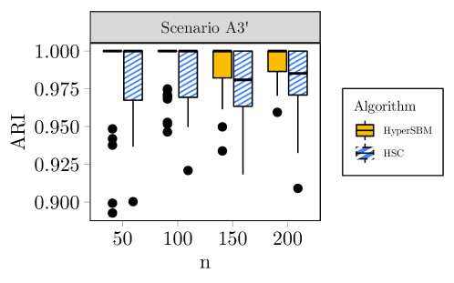
Figure 7: Boxplots of Adjusted Rand Indexes for setting A3’, for different number of nodes $n$ (along $x$-axis) and with 2 methods: our HyperSBM (left boxplot) and HSC (right boxplot).

However, setting A3 appears to be too sparse for model selection. Indeed, Table 10 shows the results of model selection in that setting, where we can see that our ICL criterion performs badly: we always under-estimate the number of groups. It is out of the scope of the present work to further explore the reasons for that nor the characterization of highly sparse wrt sparse regimes. At this point, we conclude that ICL performs well in dense settings (data not shown) as well as sparse ones, but might not in highly sparse regimes.

$Q$	$n=50$	$n=100$	$n=150$	$n=200$
1	$16\%$	$2\%$	$0\%$	$0\%$
2	$84\%$	$90\%$	$66\%$	$54\%$
3	$0\%$	$8\%$	$34\%$	$46\%$
4	$0\%$	$0\%$	$0\%$	$0\%$
5	$0\%$	$0\%$	$0\%$	$0\%$

Table 10: Frequency (as a percentage) of the selected number of groups $Q$ for scenario A3’ (true number of groups $Q=3$). Model selection is carried out by means of the ICL criterion. Results are computed over 50 samples for each value of $n$.

E.3 KS thresholds

Let us recall the expression of the Kesten-Stigum threshold for cluster detectability in symmetric $m$-uniform HSBM (which corresponds to (Aff) submodel) with equal group proportions:

$$KS_{m}=\frac{(m-1)(\alpha-\beta)^{2}}{Q^{m-1}(\alpha+(Q^{m-1}-1)\beta)}>1.$$

When the groups proportions are not uniform, we conjecture that this threshold becomes

$$\widetilde{KS}_{m}=\frac{(m-1)(\sum_{q}\pi_{q}^{m})^{2}(\alpha-\beta)^{2}}{(\sum_{q}\pi_{q}^{m})\alpha+(1-\sum_{q}\pi_{q}^{m})\beta}>1.$$

In Table 11, we indicate the values of $KS_{m},\widetilde{KS}_{m}$ in the different settings explored. We recall that those thresholds are compared to 1 and we observe values that are very small and far away from 1.

Setting A2	$n=50$	$n=100$	$n=150$	$n=200$
$KS_{2}$	1.73865e-03	8.69320e-04	5.7955e-04	4.3466e-04
$KS_{3}$	4.51728e-03	1.12932e-03	5.0192e-04	2.8233e-04
$\widetilde{KS}_{2}$	1.20957e-03	3.07650e-04	1.3753e-04	7.7590e-05
$\widetilde{KS}_{3}$	1.08160e-04	6.80000e-06	1.3400e-06	4.3000e-07
Setting A3	$n=50$	$n=100$	$n=150$	$n=200$
$KS_{2}$	3.024585e-02	1.512293e-02	1.008195e-02	7.56146e-03
$KS_{3}$	2.674160e-03	6.685400e-04	2.971300e-04	1.67130e-04
$\widetilde{KS}_{2}$	4.718480e-03	1.220110e-03	5.485500e-04	3.10350e-04
$\widetilde{KS}_{3}$	1.259000e-05	7.900000e-07	1.600000e-07	5.00000e-08
Setting A3’	$n=50$	$n=100$	$n=150$	$n=200$
$KS_{2}$	4.089033e-02	2.044517e-02	1.363011e-02	1.022258e-02
$KS_{3}$	4.998750e-03	1.249690e-03	5.554200e-04	3.124200e-04
$\widetilde{KS}_{2}$	1.624306e-02	4.319010e-03	1.961130e-03	1.115210e-03
$\widetilde{KS}_{3}$	6.353000e-05	3.990000e-06	7.900000e-07	2.500000e-07
Setting B2	$n=50$	$n=100$	$n=150$	$n=200$
$KS_{2}$	6.447368e-02	3.223684e-02	2.149123e-02	1.611842e-02
$KS_{3}$	1.238100e-04	3.095000e-05	1.376000e-05	7.740000e-06
$\widetilde{KS}_{2}$	4.049389e-02	9.110010e-03	3.918150e-03	2.168940e-03
$\widetilde{KS}_{3}$	2.160000e-06	1.400000e-07	3.000000e-08	1.000000e-08
Setting B3	$n=50$	$n=100$	$n=150$	$n=200$
$KS_{2}$	2.928695e-02	1.464348e-02	9.76232e-03	7.32174e-03
$KS_{3}$	2.800900e-04	7.002000e-05	3.11200e-05	1.75100e-05
$\widetilde{KS}_{2}$	2.431282e-02	5.605760e-03	2.42853e-03	1.34901e-03
$\widetilde{KS}_{3}$	5.700000e-06	3.600000e-07	7.00000e-08	2.00000e-08

Table 11: Values of the Kesten-Stigum thresholds in the different settings.

Appendix F Analyses on the co-authorship dataset

The original dataset has 274 papers and 314 authors, with 1 paper having 6 authors and 1 paper having 5 authors. We decided to consider $M=4$ and discard these 2 papers with more than 5 authors. Then, we looked at the largest connected component of the resulting graph. It resulted in 76 papers and 79 authors.

We ran HyperSBM with $Q$ ranging from $2$ to $5$, with 2 different initialisations: 1 random and 1 relying on the soft spectral clustering. The random initialisation always gave the best result. The results were robust to different tries. ICL selected $Q=2$ groups, as shown in Figure 8.

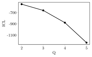
Figure 8: Integrated Classification Likelihood index resulting from fitting the HSBM to the co-authorship dataset with number of latent groups ranging from 2 to 5.

We obtained a first small group with only 8 authors (the remaining 71 authors being in the second large group). Inspecting more closely the variational parameters $\tau_{iq}$ for all the nodes, we found that a total of 4 nodes could be considered as ambiguously classified, while all other nodes had posterior probabilities to belong to one of the group larger than 0.8. More precisely, in the first small group, 2 nodes had posterior probabilities to belong to that group equal to 0.54 and 0.63, respectively; while in the second large group, 2 nodes had posterior probabilities to belong to that group equal to 0.56 and 0.72, respectively.

We discussed in the main text the number of co-authors and degrees in the bipartite graph (i.e. number of co-published papers) of the first small group of authors. We noticed that the 2 authors in this group that had smallest number of co-authors (namely 4) and smallest number of degrees (also 4) are the ones that are ambiguously clustered in this group. While the 2 other authors ambiguously clustered in the second large group have a number of co-authors of 6 and 4, respectively; and both a degree of 4. This reinforces the conclusion that on this dataset, HyperSBM has grouped apart the authors which are both the most collaborative and the most prolific ones.

Then we ran the spectral clustering algorithm on our dataset. We looked at the spectral gap, that indicated 15 groups but the gap is not clear. Then we looked at the clustering obtained with $Q=2$ groups. Spectral clustering output groups with sizes 24 and 55, respectively. We recall that spectral clustering tends to output comparable sizes groups. The small group contains the only author with 12 co-authors and the remaining authors have a number of co-authors ranging from 1 to 4. The second large group has a distribution of the number of co-authors ranging from 1 to 11. The small group contains authors with small degree in the bipartite graph, i.e having few co-published papers (all but one author have degrees less 4 and a last author has degree 7), while the second large group contains the 3 authors with largest degree, the rest of the authors having degrees ranging from 1 to 6. Thus, these groups are neither characterized by the number of co-authors nor by their degrees in the bipartite graph.

Finally, we analyzed the same dataset as a bipartite graph under a Bipartite SBM. We relied on the R package SBM through the function estimateBipartiteSBM (Chiquet et al., 2022).

The Bipartite-SBM also selected 2 groups of authors (and one group of papers). There was one small group with 4 authors, which are exactly the ones that have the highest degree in the bipartite graph and also correspond to the 4 authors having the highest number of co-authors.

Here, 2 nodes could be considered as ambiguously classified: one node from the first small (resp. second large) group had posterior probability to belong to that group of 0.73 only (resp. 0.67 only). These 2 nodes where not ambiguously classified by HyperSBM and both appeared in our first small group.

It is interesting to compare the situation of three particular authors here. Author with index 48 has 7 co-authors (the 6th highest) and 6 co-authored papers (the 5th highest). It is outside the small first group with Bipartite-SBM method (posterior probability $1-0.67=0.33$ to belong to that group); while HyperSBM clusters it unambiguously in the first small group. Similarly, author with index 27 has 12 coauthors (1st highest) and only 7 co-authored papers (the 4th highest). This node was ambiguously classified by Bipartite-SBM method in the first small group (posterior probability 0.73 only); while HyperSBM clusters it unambiguously in the first small group. Now, conversely, author with index 35 has 8 co-authors (the 6th highest) and 5 co-authored papers (also the 5th highest). This author is unambiguously clustered from the two methods; but while HyperSBM puts it in the first small graph, Bipartite-SBM excludes it from that group. The examination of these 3 particular tangent cases seem to show that on this dataset, Bipartite-SBM was more sensible to authors’s degrees in the bipartite graph while HyperSBM paid more attention to the sizes of the hyperedges (i.e. number of co-authors) an author was involved in

We also looked at estimated connection probabilities in the bipartite SBM. The authors from the first small group of Bipartite-SBM have many papers (estimated connection probability with the unique group pf papers in the bipartite graph is 11.5% whereas only 2.5% for the other large group). Finally, we computed the parameters values $B^{(m,n)}_{q_{1},\dots,q_{m}}$ obtained with the groups estimated by Bipartite-SBM. We obtained with $m=2$ that $\hat{B}^{(2)}_{11}\simeq 16,6\%$ (to be compared with $4.2\%$ in HyperSBM); while $\hat{B}^{(2)}_{12}\simeq 7\%$ and $\hat{B}^{(2)}_{22}\simeq 1\%$ (more similar to the results of HyperSBM, which are $5.1\%$ and $0.8\%$, respectively). In this case, the first group of authors behaves differently with respect to within-group connections compared to between-group connections.

References

- Ahn et al. (2018) Ahn, K., K. Lee, and C. Suh (2018). Hypergraph spectral clustering in the weighted stochastic block model. IEEE J Sel Top Signal Process 12(5), 959–974.
- Allman et al. (2011) Allman, E., C. Matias, and J. Rhodes (2011). Parameters identifiability in a class of random graph mixture models. Journal Statist Plann Inf 141, 1719–1736.
- Angelini et al. (2015) Angelini, M. C., F. Caltagirone, F. Krzakala, and L. Zdeborová (2015). Spectral detection on sparse hypergraphs. In 2015 53rd Annual Allerton Conference on Communication, Control, and Computing (Allerton), pp. 66–73.
- Balasubramanian (2021) Balasubramanian, K. (2021). Nonparametric modeling of higher-order interactions via hypergraphons. J Mach Learn Res 22(146), 1–35.
- Battiston et al. (2020) Battiston, F., G. Cencetti, I. Iacopini, V. Latora, M. Lucas, A. Patania, J.-G. Young, and G. Petri (2020). Networks beyond pairwise interactions: Structure and dynamics. Phys Rep 874, 1–92.
- Behrens et al. (2013) Behrens, S., C. Erbes, M. Ferrara, S. G. Hartke, B. Reiniger, H. Spinoza, and C. Tomlinson (2013). New results on degree sequences of uniform hypergraphs. Electron J Comb 20(4), research paper p14, 18.
- Bick et al. (2021) Bick, C., E. Gross, H. A. Harrington, and M. T. Schaub (2021). What are higher-order networks? Technical report, arXiv:2104.11329.
- Biernacki et al. (2000) Biernacki, C., G. Celeux, and G. Govaert (2000). Assessing a mixture model for clustering with the Integrated Completed Likelihood. IEEE Trans Pattern Anal Machine Intel 22(7), 719–725.
- Cafieri et al. (2010) Cafieri, S., P. Hansen, and L. Liberti (2010). Loops and multiple edges in modularity maximization of networks. Phys Rev E 81, 046102.
- Chelaru et al. (2021) Chelaru, M. I., S. Eagleman, A. R. Andrei, R. Milton, N. Kharas, and V. Dragoi (2021). High-order correlations explain the collective behavior of cortical populations in executive, but not sensory areas. Neuron 109(24), 3954–3961.
- Chien et al. (2019) Chien, I. E., C.-Y. Lin, and I.-H. Wang (2019). On the minimax misclassification ratio of hypergraph community detection. IEEE Trans Inf Theory 65(12), 8095–8118.
- Chiquet et al. (2022) Chiquet, J., S. Donnet, großBM team, and P. Barbillon (2022). sbm: Stochastic Blockmodels. R package version 0.4.4.
- Chodrow (2020) Chodrow, P. S. (2020). Configuration models of random hypergraphs. J Complex Networks 8(3), cnaa018.
- Chodrow et al. (2021) Chodrow, P. S., N. Veldt, and A. R. Benson (2021). Generative hypergraph clustering: From blockmodels to modularity. Sci Adv 7(28), eabh1303.
- Cole and Zhu (2020) Cole, S. and Y. Zhu (2020). Exact recovery in the hypergraph stochastic block model: A spectral algorithm. Linear Algebra Appl 593, 45–73.
- Dempster et al. (1977) Dempster, A., N. Laird, and D. Rubin (1977). Maximum likelihood from incomplete data via the EM algorithm (with discussion). J R Stat Soc, Ser B 39, 1–38.
- Estrada and Rodríguez-Velázquez (2006) Estrada, E. and J. A. Rodríguez-Velázquez (2006). Subgraph centrality and clustering in complex hyper-networks. Physica A 364, 581–594.
- Frank and Harary (1982) Frank, O. and F. Harary (1982). Cluster inference by using transitivity indices in empirical graphs. J Amer Statist Assoc 77(380), 835–840.
- Ghoshal et al. (2009) Ghoshal, G., V. Zlatić, G. Caldarelli, and M. E. J. Newman (2009). Random hypergraphs and their applications. Phys Rev E 79, 066118.