Boosting the Transferability of Adversarial Attacks with Reverse Adversarial Perturbation

Abstract

Deep neural networks (DNNs) have been shown to be vulnerable to adversarial examples, which can produce erroneous predictions by injecting imperceptible perturbations. In this work, we study the transferability of adversarial examples, which is significant due to its threat to real-world applications where model architecture or parameters are usually unknown. Many existing works reveal that the adversarial examples are likely to overfit the surrogate model that they are generated from, limiting its transfer attack performance against different target models. To mitigate the overfitting of the surrogate model, we propose a novel attack method, dubbed reverse adversarial perturbation (RAP). Specifically, instead of minimizing the loss of a single adversarial point, we advocate seeking adversarial example located at a region with unified low loss value, by injecting the worst-case perturbation (i.e., the reverse adversarial perturbation) for each step of the optimization procedure. The adversarial attack with RAP is formulated as a min-max bi-level optimization problem. By integrating RAP into the iterative process for attacks, our method can find more stable adversarial examples which are less sensitive to the changes of decision boundary, mitigating the overfitting of the surrogate model. Comprehensive experimental comparisons demonstrate that RAP can significantly boost adversarial transferability. Furthermore, RAP can be naturally combined with many existing black-box attack techniques, to further boost the transferability. When attacking a real-world image recognition system, i.e., Google Cloud Vision API, we obtain 22% performance improvement of targeted attacks over the compared method. Our codes are available at: https://github.com/SCLBD/Transfer_attack_RAP.

1 Introduction

Deep neural networks (DNNs) have been successfully applied in many safety-critical tasks, such as autonomous driving, face recognition and verification, etc. However, it has been shown that DNN models are vulnerable to adversarial examples [35, 12, 27, 9, 44, 50, 45, 32], which are indistinguishable from natural examples but make a model produce erroneous predictions. For real-world applications, the DNN models are often hidden from users. Therefore, the attackers need to generate the adversarial examples under black-box setting where they do not know any information of the target model [2, 3, 18, 32]. For black-box setting, the adversarial transferability matters since it can allow the attackers to attack target models by using adversarial examples generated on the surrogate models. Therefore, learning how to generate adversarial examples with high transferability has gained more attentions in the literature [26, 38, 5, 48, 14, 10, 23].

Under white-box setting where the complete information of the attacked model (e.g., architecture and parameters) is available, the gradient-based attacks such as PGD [27] have demonstrated good attack performance. However, they often exhibit the poor transferiability [48, 5], i.e., the adversarial example $\bm{x}^{adv}$ generated from the surrogate model $\mathcal{M}^{S}$ performs poorly against different target models $\mathcal{M}^{T}$. The previous works attribute that to the overfitting of adversarial examples to the surrogate models [5, 48, 24]. Figure 1 (b) gives an illustration. The PGD attack aims to find an adversarial point $\bm{x}^{pgd}$ with minimal attack loss, while doesn’t consider the attack loss of the neighborhood regions round $\bm{x}^{pgd}$. Due to the highly non-convex of deep models, when $\bm{x}^{pgd}$ locates at a sharply local minimum, a slight change on model parameters of $\mathcal{M}^{S}$ could cause a large increase of the attack loss, making $\bm{x}^{pgd}$ fail to attack the perturbed model.

Many techniques have been proposed to mitigate the overfitting and improve the transferability, including input transformation [6, 48], gradient calibration [14], feature-level attacks [17], and generative models [30], etc. However, there still exists a large gap of attack performance between the transfer setting and the ideal white-box setting, especially for targeted attack, requiring more efforts for boosting the transferability.

In this work, we propose a novel attack method called reverse adversarial perturbation (RAP) to alleviate the overfitting of the surrogate model and boost the transferability of adversarial examples. We encourage that $\bm{x}^{adv}$ is not only of low attack loss but also locates at a local flat region, i.e., the points within the local neighborhood region around $\bm{x}^{adv}$ should also be of low loss values. Figure 1 (b) illustrates the difference between the sharp local minimum and flat local minimum. When the model parameter of $\mathcal{M}^{S}$ has some slight changes, the variation of the attack loss w.r.t. the flat local minimum is less than that of the sharp one. Therefore, the flat local minimum is less sensitive to the changes of decision boundary. To achieve this goal, we formulate a min-max bi-level optimization problem. The inner maximization aims to find the worst-case perturbation (i.e., that with the largest attack loss, and this is why we call it reverse adversarial perturbation) within the local region around the current adversarial example, which can be solved by the projected gradient ascent algorithm. Then, the outer minimization will update the adversarial example to find a new point added with the provided reverse perturbation that leads to lower attack loss. Figure 1 (a) provides an illustration of the optimization process. For $t$-th iteration and $\bm{x}^{t}$, RAP first finds the point $\bm{x}^{t}+\bm{n}^{rap}$ with max attack loss within the neighborhood region of $\bm{x}^{t}$. Then it updates $\bm{x}^{t}$ with the gradient calculated by minimizing the attack loss w.r.t. $\bm{x}^{t}+\bm{n}^{rap}$. Compared to directly adopting the gradient at $\bm{x}^{t}$, RAP could help escape from the sharp local minimum and pursue a relatively flat local minimum. Besides, we design a late-start variant of RAP (RAP-LS) to further boost the attack effectiveness and efficiency, which doesn’t insert the reverse perturbation into the optimization procedure in the early stage. Moreover, from the technical perspective, since the proposed RAP method only introduces one specially designed perturbation onto adversarial attacks, one notable advantage of RAP is that it can be naturally combined with many existing black-box attack techniques to further boost the transferability. For example, when combined with different input transformations (e.g., the random resizing and padding in Diverse Input [48]), our RAP method consistently outperforms the counterparts by a clear margin.

Our main contributions are three-fold: 1) Based on a novel perspective, the flatness of loss landscape for adversarial examples, we propose a novel adversarial attack method RAP that encourages both the adversarial example and its neighborhood region be of low loss value; 2) we present a vigorous experimental study and show that RAP can significantly boost the adversarial transferability on both untargeted and targeted attacks for various networks also containing defense models; 3) we demonstrate that RAP can be easily combined with existing transfer attack techniques and outperforms the state-of-the-art performance by a large margin.

2 Related Work

The black-box attacks can be categorized into two categories: 1) query-based attacks that conduct the attack based on the feedback of iterative queries to target models, and 2) transfer attacks that use the adversarial examples generated on some surrogate models to attack the target models. In this work, we focus on the transfer attacks. For surrogate models, existing attack algorithms such as FGSM [12] and I-FGSM [21] could achieve good attack performance. However, they often overfit the surrogate models and thus exhibit poor transferability. Recently, many works have been proposed to generate more transferable adversarial examples [5, 48, 24, 6, 41, 39, 40, 43, 14, 17, 19, 20, 13], which we briefly summarize as below.

Input transformation: Data augmentation, which has been shown to be effective in improving model generalization, has also been studied to boost the adversarial transferability, such as randomly resizing and padding [48], randomly scaling [24], and adversarial mixup [41]. In addition, the work of Dong et al. [6] uses a set of translated images to compute gradient and get the better performance against defense models. Expectation of Transformation (EOT) method [1] synthesizes adversarial examples over a chosen distribution of transformations to enhance its adversarial transferability. Gradient modification: Instead of the I-FGSM, the work of Dong et al. [5] integrates momentum into the updating strategy. And Lin et al. [24] uses the Nesterov accelerated gradient to boost the transferability. The work of Wang and He [40] aims to find a more stable gradient direction by tuning the variance of each gradient step. There are also some model-specific designs to boost the adversarial transferability. For example, Wu et al. [43] found that the gradient of skip connections is more crucial to generate more transferable attacks. The work of Guo et al. [14] proposed LinBP to utilize more gradient of skip connections during the back-propagation. However, these methods tend to be specific to a particular model architecture, such as skip connection, and it is nontrivial to extend the findings to other architectures or modules. Intermediate feature attack: Meanwhile, Huang et al. [17], Inkawhich et al. [19, 20] proposed to exploit feature space constraints to generate more transferable attacks. Yet they need to identity the best performing intermediate layers or train one-vs-all binary classifies for all attacked classes. Recently, Zhao et al. [49] find iterative attacks with much more iterations and logit loss can achieve relatively high targeted transferability and exceed the feature-based attacks. Generative models: In addition, there have been some methods utilizing the generative models to generate the adversarial perturbations [31, 28, 30]. For example, the work of Naseer et al. [30] proposed to train a generative model to match the distributions of source and target class, so as to increase the targeted transferability. However, the learning of the perturbation generator is nontrivial, especially on large-scale datasets.

In summary, the current performance of transfer attacks is still unsatisfactory, especially for targeted attacks. In this work, we study adversarial transferability from the prespective of the flatness of adversarial examples. We find that adversarial examples located at flat local minimum will be more transferable than those at sharp local minimum and propose an novel algorithm to find adversarial example that locates at flat local minimum.

3 Methodology

3.1 Preliminaries of Transfer Adversarial Attack

Given an benign sample $(\bm{x},y)\in(\mathcal{X},\mathcal{Y})$, the procedure of transfer adversarial attack is firstly constructing the adversarial example $\bm{x}^{adv}$ within the neighborhood region $\mathcal{B}_{\epsilon}(\bm{x})=\{\bm{x}^{\prime}:\|\bm{x}^{\prime}-\bm{x}\|_{p}\leq\epsilon\}$ by attacking the white-box surrogate model $\mathcal{M}^{s}(\bm{x};\bm{\theta}):\mathcal{X}\rightarrow\mathcal{Y}$, then transferring $\bm{x}^{adv}$ to directly attack the black-box target model $\mathcal{M}^{t}(\bm{x};\bm{\phi}):\mathcal{X}\rightarrow\mathcal{Y}$. The attack goal is to mislead the target model, i.e., $\mathcal{M}^{t}(\bm{x}^{adv};\bm{\phi})\neq y$ (untargeted attack), or $\mathcal{M}^{t}(\bm{x}^{adv};\bm{\phi})=y_{t}$ (targeted attack) with $y_{t}\in\mathcal{Y}$ indicting the target label. Taking the target attack as example, the general formulation of many existing transfer attack methods can be written as follows:

$$\min_{\bm{x}^{adv}\in\mathcal{B}_{\epsilon}(\bm{x})}\mathcal{L}(\mathcal{M}^{s}(\mathcal{G}(\bm{x}^{adv});\bm{\theta}),y_{t}).$$ (1)

The loss function $\mathcal{L}$ is often set as the cross entropy (CE) loss [48] or the logit loss [49], which will be specified in later experiments. Besides, the formulation of untargeted attack can be easily obtained by replacing the loss function $\mathcal{L}$ and $y_{t}$ by $-\mathcal{L}$ and $y$, respectively.

Since $\mathcal{M}^{s}$ is white-box, if $\mathcal{G}(\cdot)$ is set as the identity function, then any off-the-shelf white-box adversarial attack method can be adopted to solve Problem (1), such as I-FSGM [21], MI-FGSM [5], etc. Meanwhile, existing works have designed different $\mathcal{G}(\cdot)$ functions and developed the corresponding optimization algorithms, to boost the adversarial transferability between surrogate and target models. For example, $\mathcal{G}(\cdot)$ is specified as random resizing and padding (DI) [48], translation transformation (TI) [6], scale transformation (SI) [24], and adversarial mixup (Admix) [41].

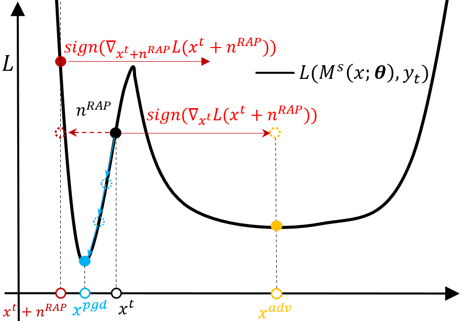
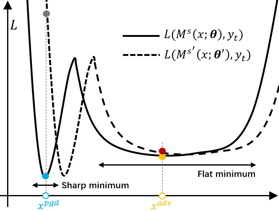
Figure 1: These two plots are schematic diagrams in 1D space. The x-axis means the value of input $\bm{x}$. The y-axis means the value of attack loss function $\mathcal{L}$. (a) Illustration of our attack method and the original PGD attack. (b) Illustration of attack loss landscape of $\mathcal{M}^{S}$ and $\mathcal{M}^{S^{\prime}}$. $\mathcal{M}^{S^{\prime}}$ denotes a slight change on the model parameters of $\mathcal{M}^{S}$. The blue and yellow dots correspond to attacks located at different local minima on $\mathcal{M}^{S}$, respectively. The gray and red points are their counterparts on $\mathcal{M}^{S^{\prime}}$.

3.2 Reverse Adversarial Perturbation

As discussed above, although having good performance for the white-box setting, the adversarial examples generated from $\mathcal{M}^{S}$ exist poor adversarial transferability on $\mathcal{M}^{T}$, especially for targeted attacks. The previous works attribute this issue to the overfitting of adversarial attack to $\mathcal{M}^{S}$ [5, 46, 38, 6, 4]. As shown in Figure 1 (b), when $\bm{x}^{pgd}$ locates at a sharp local minimum, it is not stable and is sensitive to changes of $\mathcal{M}^{S}$. When having some changes on model parameters, $\bm{x}^{pgd}$ could results in a high attack loss against $\mathcal{M}^{S^{\prime}}$ and lead to a failure attack.

To mitigating the overfitting to $\mathcal{M}^{S}$, we advocate to find $\bm{x}^{adv}$ located at flat local region. That means we encourage that not only $\bm{x}^{adv}$ itself has low loss value, but also the points in the vicinity of $\bm{x}^{adv}$ have similarly low loss values.

To this end, we propose to minimize the maximal loss value within a local neighborhood region around the adversarial example $\bm{x}^{adv}$. The maximal loss is implemented by perturbing $\bm{x}^{adv}$ to maximize the attack loss, named Reverse Adversarial Perturbation (RAP). By inserting the RAP into the formulation (1), we aim to solve the following problem,

$$\min_{\bm{x}^{adv}\in\mathcal{B}_{\epsilon}(\bm{x})}\mathcal{L}(\mathcal{M}^{s}(\mathcal{G}(\bm{x}^{adv}+\bm{n}^{rap});\bm{\theta}),y_{t}),$$ (2)

where

$$\bm{n}^{rap}=\underset{\|\bm{n}^{rap}\|_{\infty}\leq\epsilon_{n}}{\arg\max}\mathcal{L}(\mathcal{M}^{s}(\bm{x}^{adv}+\bm{n}^{rap};\bm{\theta}),y_{t}),$$ (3)

with $\bm{n}^{rap}$ indicating the RAP, and $\epsilon_{n}$ defining its search region. The above formulations (2) and (3) correspond to the targeted attack, and the corresponding untargeted formulations can be easily obtained by replacing the loss function $\mathcal{L}$ and $y_{t}$ by $-\mathcal{L}$ and $y$, respectively.

It is a min-max bi-level optimization problem [25], and can be solved by iteratively optimizing the inner maximization and the outer minimization problem. Specifically, in each iteration, given $\bm{x}^{adv}$, the inner maximization w.r.t. $\bm{n}^{rap}$ is solved by the projected gradient ascent algorithm:

$$\bm{n}^{rap}\leftarrow\bm{n}^{rap}+\alpha_{n}\cdot\text{sign}(\nabla_{\bm{n}^{rap}}\mathcal{L}(\mathcal{M}^{s}(\bm{x}^{adv}+\bm{n}^{rap};\bm{\theta}),y_{t})).$$ (4)

The above update is conducted by $T$ steps, and $\alpha_{n}=\frac{\epsilon_{n}}{T}$. Then, given $\bm{n}^{rap}$, the outer minimization w.r.t. $\bm{x}^{adv}$ can be solved by any off-the-shelf algorithm that is developed for solving (1). For example, it can be undated by one step projected gradient descent, as follows:

$$\bm{x}^{adv}\leftarrow\text{Clip}_{\mathcal{B}_{\epsilon}(\bm{x})}\big{[}\bm{x}^{adv}-\alpha\cdot\text{sign}(\nabla_{\bm{x}^{adv}}\mathcal{L}(\mathcal{M}^{s}(\mathcal{G}(\bm{x}^{adv}+\bm{n}^{rap});\bm{\theta}),y_{t}))\big{]},$$ (5)

with $\text{Clip}_{\mathcal{B}_{\epsilon}(\bm{x})}(\bm{a})$ clipping $\bm{a}$ into the neighborhood region $\mathcal{B}_{\epsilon}(\bm{x})$. The overall optimization procedure is summarized in Algorithm 1. Moreover, since the optimization w.r.t. $\bm{x}^{adv}$ can be implemented by any off-the-shelf algorithm for solving Problem (1), one notable advantage of the proposed RAP is that it can be naturally combined with any one of them, such as the input transformation methods [48, 6, 24, 41].

A Late-Start (LS) Variant of RAP.

In our preliminary experiments, we find that RAP requires more iterations to converge and the performance is slightly lower during the initial iterations, compared to its baseline attack methods. As shown in Figure 2, we combine MI [5] and Admix [41] with RAP, and adopt ResNet-50 as the surrogate model. We take the evaluation on 1000 images from ImageNet (see Sec.4.1). It is observed that the method with RAP (see the orange curves) quickly surpasses its baseline method (see the blue curves) and finally achieves much higher success rate with more iterations, which verify the effect of RAP on enhancing the adversarial transferability. However, it is also observed that the performance of RAP is slightly lower than its baseline method in the early stage. The possible reason is that the early-stage attack is of very weak attack performance to the surrogate model. In this case, it may be waste to pursue better transferable attacks by solving the min-max problem. A better strategy may be only solving the minimization problem (1) in the early stage to quickly achieve the region of relatively high adversarial attack performance, then starting RAP to further enhance the attack performance and transferability simultaneously. This strategy is denoted as RAP with late-start (RAP-LS), whose effect is preliminarily supported by the results shown in Figure 2 (see the green curve) and will be evaluated extensively in later experiments.

3.3 A Closer Look at RAP

To verify whether RAP can help us find a $\bm{x}^{adv}$ located at the local flat region or not, we use ResNet-50 as surrogate model and conduct the untargeted attacks. We visualize the loss landscape around $\bm{x}^{adv}$ on $\mathcal{M}^{S}$ by plotting the loss variations when we move $\bm{x}^{adv}$ along a random direction with different magnitudes $a$. The details of the calculation are provided in Appendix. Figure 3 plots the visualizations. We take I-FGSM [21] (denoted as I), MI [5], DI [48], and MI-TI-DI (MTDI) as baselines attacks and combined them with RAP. We can see that comparing to the baselines, RAP could help find $\bm{x}^{adv}$ located at the flat region.

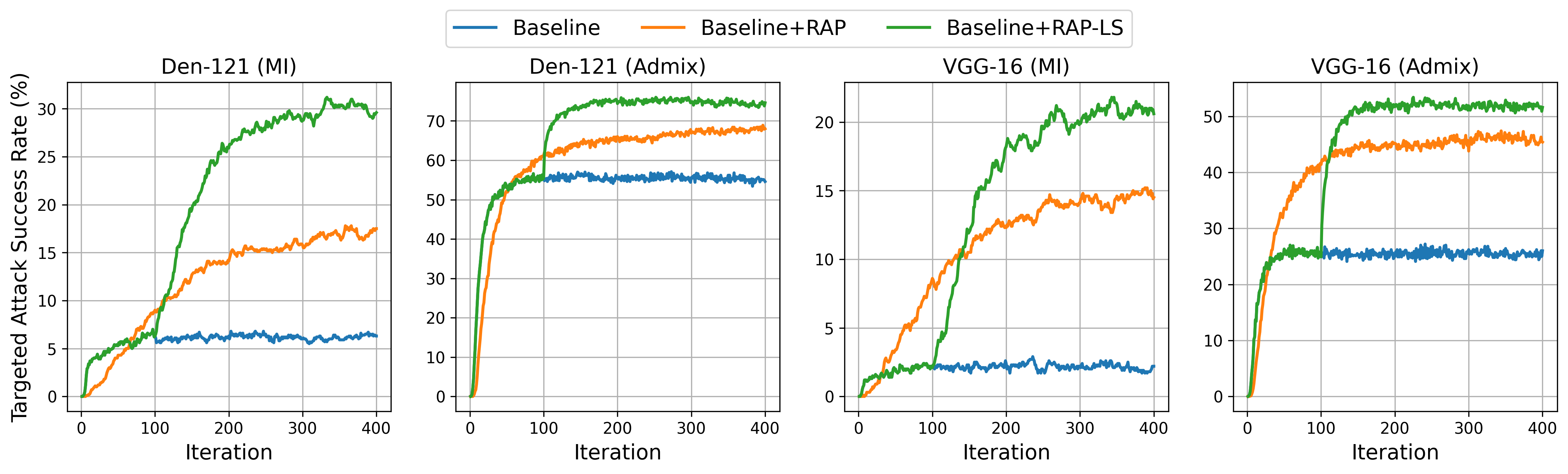
Figure 2: Targeted attack success rate ($\%$) on Dense-121 and VGG-16. We take the Res-50 as the surrogate model and take MI and Admix as baseline methods.

Algorithm 1 Reverse Adversarial Perturbation (RAP) Algorithm

Input: Surrogate model $\mathcal{M}^{s}$, benign data $(\bm{x},y)$, target label $y_{t}$, loss function $\mathcal{L}$, transformation $\mathcal{G}$, the global iteration number $K$, the late-start iteration number $K_{LS}$ of RAP, as well as hyper-parameters in optimization (specified in later experiments) Output: the adversarial example $\bm{x}^{adv}$

1:  Initialize $\bm{x}^{adv}\leftarrow\bm{x}$

2:  for $k=1,\dots,K$ do

3:     if $k\geq K_{LS}$ then

4:        Initialize $\bm{n}^{rap}\leftarrow\bm{0}$

5:        for $t=1,\dots,T$ do

6:           Update $\bm{n}^{rap}$ using (4)

7:     Update $\bm{x}^{adv}$ using (5)

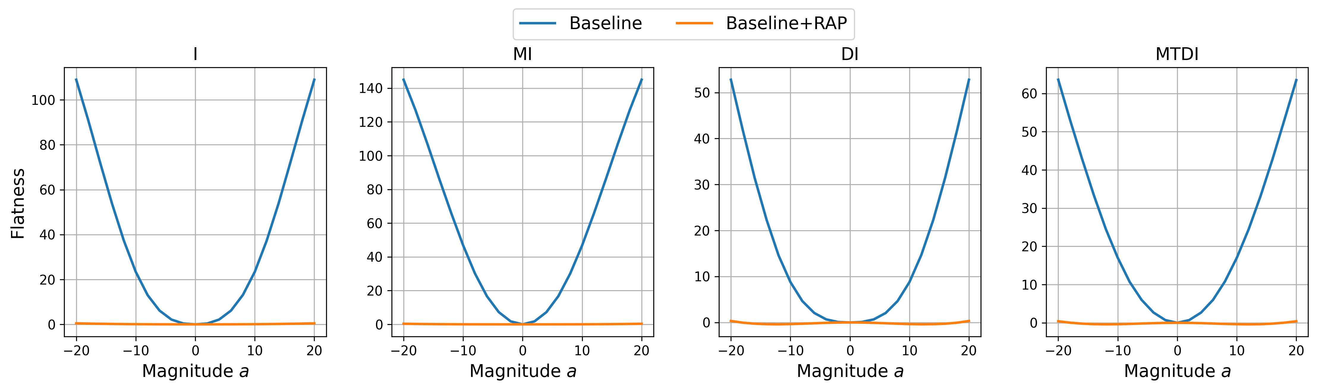
Figure 3: The flatness visualization of untargeted adversarial examples on $\mathcal{M}^{S}$. The implementation details are shown in Section B of Appendix.

4 Experiments

4.1 Experimental Settings

Dataset and Evaluated Models. We conduct the evaluation on the ImageNet-compatible dataset comprised of 1,000 images. For the surrogate models, we consider the four widely used network architectures: Inception-v3 (Inc-v3) [36], ResNet-50 (Res-50) [15], DenseNet-121 (Dense-121) [16], and VGG-16bn (VGG-16) [34]. For target models, apart from the above models, we also utilize more diverse architectures: Inception-ResNet-v2 (Inc-Res-v2) [37], NASNet-Large (NASNet-L) [51], and ViT-Base/16 (ViT-B/16) [8]. For defense models, we adopt the two widely used ensemble adversarial training (AT) models: adv-Inc-v3 (Inc-v3_adv) and ens-adv-Inc-Res-v2 (IncRes-v2_ens) [38]. Besides, we also test multi-step AT model [33], imput transformation defense [46], feature denoising [47], and purification defense (NRP) [29].

Compared Methods. We adopt I-FGSM [21] (denoted as I), MI [5], TI [6], DI [48], SI [24], Admix [41], VT [40], EMI [42], ILA [17], LinBP [14], Ghost Net [22], and the generative targeted attack method TTP [30]. We also consider the combination of baseline methods, including MI-TI-DI (MTDI), MI-TI-DI-SI (MTDSI), and MI-TI-DI-Admix (MTDAI). Besides, Expectation of Transformation (EOT) method [1] is also a comparable baseline method. We also conduct the comparison of RAP and EOT.

Implementation Details. For untargeted attack, we adopt the Cross Entropy (CE) loss. For targeted attack, apart from CE, we also experiment with the logit loss, where Zhao et al. [49] shows it behaves better for targeted attack. The adversarial perturbation $\epsilon$ is restricted by $\ell_{\infty}=16/255$. The step size $\alpha$ is set as $2/255$ and number of iteration $K$ is set as $400$ for all attacks. In the following, we mainly show the results at $K=400$ and the results at different value of $K$ are shown in Appendix. For RAP, we set $K_{LS}$ as $100$ and $\alpha_{n}$ as $2/255$. We set $\epsilon_{n}$ as $12/255$ for I and TI in untargeted attack and $16/255$ for other attacks in all other settings. The computational cost is shown in Section B of Appendix.

Extra Experiments in Appendix. Due to the space limitation, we put extra experiment results in Appendix. The comparisons of RAP and EOT, VT, EMI, and Ghost Net methods are shown in Section C in Appendix. The evaluation of RAP on stronger defense model, multi-step AT models, NRP, and feature denoising, is shown in Section D. The evaluation of ensemble-model attacks on these diverse network architectures is given in Section E.2.

4.2 The Evaluation of Untargeted Attacks

Baseline Methods. We first evaluate the performance of RAP and RAP-LS with different baseline attacks, including I, MI, DI, TI, SI, and Admix. The results are shown in Table 1. For instance, the ‘MI/ +RAP/ +RAP-LS’ denotes the methods of baseline MI, MI+RAP, and MI+RAP-LS, respectively. RAP achieves the significant improvements for all methods on each target model. For average attack success rate of all target models, RAP outperforms the I and MI by $9.6\%$ and $16.3\%$, respectively. For TI, DI, SI, and Admix, RAP gets the improvements by $10.2\%$, $10.9\%$, $9.3\%$, and $6.3\%$. With late-start, RAP-LS further enhance the transfer attack performance for almost all methods.

Combinational Methods. Prior works demonstrate the combination of baseline methods could largely boost the adversarial transferability [49, 41]. We also investigate of behavior of RAP when incorporated with the combinational attacks. The results are shown in Table 2. As shown in the table, there exist the clear improvements of the combinational attacks over all baseline attacks shown in Table 1. In addition, our RAP-LS further boosts the average attack success rate of the three combinational attacks by $6.9\%$, $2.6\%$, and $1.7\%$ respectively. Combined with the three combinational attacks, RAP-LS achieves $95.4\%$, $97.6\%$, and $98.3\%$ average attack success rate, respectively. These results demonstrate RAP can significantly enhance the transferability.

Table 1: The untargeted attack success rate ($\%$) of baseline attacks with RAP. The results with $CE$ loss are reported. The best results are bold and the second best results are underlined.

Attack		ResNet-50 $\Longrightarrow$			DenseNet-121$\Longrightarrow$
	Dense-121	VGG-16	Inc-v3	Res-50	VGG-16	Inc-v3
I / +RAP / +RAP-LS	79.2 / 91.5 / 91.9	78.0 / 91.1 / 92.9	34.6 / 57.0 / 57.2	87.4 / 94.2 / 94.3	85.1 / 91.7 / 92.8	46.5 / 60.2 / 61.1
MI / +RAP / +RAP-LS	85.8 / 95.0 / 96.1	82.4 / 93.9 / 94.5	50.3 / 75.9 / 77.4	90.3 / 97.6 / 97.9	87.5 / 96.0 / 97.6	59.3 / 80.4 / 82.8
TI / +RAP / +RAP-LS	82.0 / 94.1 / 95.1	81.0 / 93.1 / 93.3	45.5 / 66.1 / 67.0	89.6 / 94.2 / 94.8	87.0 / 92.1 / 93.3	54.2 / 66.7 / 70.0
DI / +RAP / +RAP-LS	99.0 / 99.6 / 99.7	99.0 / 99.6 / 99.7	57.7 / 82.9 / 85.0	98.2 / 99.6 / 99.7	98.1 / 99.4 / 99.4	67.6 / 86.6 / 86.9
SI / +RAP / +RAP-LS	94.9 / 98.9 / 99.7	88.6 / 95.7 / 97.2	65.9 / 79.7 / 84.4	95.1 / 96.9 / 98.8	91.9 / 95.0 / 97.5	71.6 / 83.2 / 87.4
Admix / +RAP / +RAP-LS	97.9 / 99.6 / 99.9	95.8 / 97.7 / 99.0	77.7 / 87.4 / 92.6	97.0 / 99.0 / 99.2	95.6 / 97.7 / 98.6	82.0 / 89.8 / 93.8
Attack		VGG-16 $\Longrightarrow$			Inc-v3$\Longrightarrow$
	Res-50	Dense-121	Inc-v3	Res-50	Dense-121	VGG-16
I / +RAP / +RAP-LS	53.7 / 53.0 / 54.2	49.1 / 50.6 / 51.4	22.0 / 24.7 / 24.9	51.5 / 62.1 / 62.0	48.7 / 60.8 / 60.0	55.1 / 65.9 / 68.0
MI / +RAP / +RAP-LS	62.5 / 76.2 / 76.4	60.5 / 73.0 / 73.9	30.0 / 42.7 / 42.2	62.0 / 85.8 / 84.8	56.7 / 84.6 / 84.6	63.1 / 84.9 / 84.6
TI / +RAP / +RAP-LS	62.8 / 64.8 / 65.8	55.9 / 63.7 / 62.1	29.1 / 36.2 / 37.1	49.3 / 63.4 / 61.6	49.4 / 63.4 / 63.8	58.1 / 68.6 / 69.5
DI / +RAP / +RAP-LS	72.2 / 86.0 / 88.8	68.8 / 85.0 / 87.4	29.9 / 46.6 / 51.6	68.4 / 81.7 / 81.8	71.9 / 85.0 / 84.0	76.1 / 85.2 / 86.4
SI / +RAP / +RAP-LS	80.0 / 92.7 / 94.7	82.1 / 94.8 / 95.7	45.8 / 74.0 / 74.7	66.2 / 69.8 / 72.8	65.9 / 74.9 / 77.2	66.0 / 69.2 / 73.0
Admix / +RAP / +RAP-LS	87.3 / 94.6 / 96.8	88.2 / 96.4 / 97.2	55.5 / 77.6 / 80.8	75.9 / 80.2 / 84.9	78.5 / 83.7 / 87.4	74.5 / 77.2 / 83.5

Table 2: The untargeted attack success rate ($\%$) of combinational methods with RAP. The results with $CE$ loss are reported. The best results are bold and the second best results are underlined.

Attack		ResNet-50 $\Longrightarrow$			DenseNet-121$\Longrightarrow$
	Dense-121	VGG-16	Inc-v3	Res-50	VGG-16	Inc-v3
MTDI / +RAP / +RAP-LS	99.8 / 100 / 100	99.8 / 100 / 99.9	85.7 / 96.0 / 96.9	99.4 / 99.8 / 100	99.2 / 99.5 / 100	89.1 / 97.1 / 97.1
MTDSI / +RAP / +RAP-LS	100 / 100 / 100	99.7 / 99.9 / 99.8	97.0 / 99.1 / 99.1	99.8 / 99.9 / 99.9	99.2 / 99.3 / 99.7	95.1 / 98.3 / 98.4
MTDAI / +RAP / +RAP-LS	100 / 100 / 100	99.8 / 99.9 / 99.9	98.3 / 99.2 / 99.8	99.8 / 99.8 / 99.9	99.4 / 99.6 / 99.8	97.9 / 98.8 / 98.9
Attack		VGG-16 $\Longrightarrow$			Inc-v3$\Longrightarrow$
	Res-50	Dense-121	Inc-v3	Res-50	Dense-121	VGG-16
MTDI / +RAP / +RAP-LS	90.0 / 97.2 / 97.7	88.8 / 97.0 / 97.3	56.8 / 82.6 / 81.4	82.9 / 91.8 / 90.6	85.7 / 94.2 / 93.3	85.1 / 92.7 / 91.0
MTDSI / +RAP / +RAP-LS	97.6 / 98.8 / 99.4	98.1 / 99.2 / 99.4	85.0 / 94.1 / 95.2	89.0 / 91.2 / 92.3	92.0 / 95.2 / 95.6	87.6 / 90.3 / 92.2
MTDAI / +RAP / +RAP-LS	97.8 / 99.2 / 99.6	98.9 / 99.5 / 99.6	89.3 / 95.0 / 95.5	91.5 / 94.1 / 94.7	95.4 / 96.2 / 97.6	91.4 / 93.2 / 94.1

4.3 The Evaluation of Targeted Attacks

We then evaluate the targeted attack performance of the different methods with RAP. The results with logit loss are presented and the results with CE loss are shown in Appendix.

Baseline Methods. The results of RAP with baseline attacks are shown in Table 3. From the results, RAP is also very effective in enhancing the transferability in targeted attacks. Taking ResNet-50 and DenseNet-121 as surrogate models for example, the average performance improvements induced by RAP are $5.0\%$ (I), $8.1\%$ (MI), $4.6\%$ (TI), $10.4\%$ (DI), $18.5\%$ (SI), and $15.1\%$ (Admix), respectively. Comparing to the ResNet-50 and DenseNet-121, the baseline attacks generally achieve lower transferability when using the VGG-16 or Inception-v3 as the surrogate models, which has also been verified in existing works [48, 49]. However, for Inception-v3 and VGG-16 as the surrogate models, RAP also consistently boosts the transferability under all cases. With late-start, RAP-LS could further improve the transferability of RAP for most attacks. The average attack success rate under all attack cases of RAP-LS is $2.6\%$ higher than that of RAP.

Combinational Methods. As did in the untargeted attacks, we also evaluate the performance of combinational methods. The results are shown in Table 4. Similar to the findings in untargeted attacks, the combinational methods obtain significantly improvements over baseline methods. The RAP-LS outperforms all combinational methods by a significantly margin. For example, taking the average attack success rate of all target models as evaluation metric, RAP-LS obtains $14.2\%$, $11.8\%$, $9.3\%$ improvements over the MTDI, MTDSI and MTDAI, respectively.

Table 3: The targeted attack success rate ($\%$) of baseline methods with RAP. The results with logit loss are reported. The best results are bold and the second best results are underlined.

Attack		ResNet-50 $\Longrightarrow$			DenseNet-121$\Longrightarrow$
	Dense-121	VGG-16	Inc-v3	Res-50	VGG-16	Inc-v3
I / +RAP / +RAP-LS	4.5 / 9.5 / 14.3	2.4 / 9.8 / 11.8	0.1 / 0.1 / 0.7	5.0 / 12.8 / 17.9	2.9 / 10.1 / 15.9	0.0 / 0.8 / 1.2
MI / +RAP / +RAP-LS	6.3 / 17.5 / 29.6	2.2 / 14.5 / 20.6	0.1 / 1.1 / 2.4	4.6 / 16.2 / 26.5	3.1 / 13.4 / 23.2	0.3 / 2.0 / 3.4
TI / +RAP / +RAP-LS	7.2 / 11.0 / 17.3	4.0 / 12.9 / 15.3	0.1 / 0.8 / 1.2	8.4 / 13.5 / 20.8	5.2 / 12.4 / 16.4	0.2 / 2.1 / 3.0
DI / +RAP / +RAP-LS	62.6 / 64.9 / 73.9	57.2 / 63.4 / 69.3	1.5 / 7.9 / 10.1	30.2 / 52.6 / 60.4	32.1 / 49.5 / 58.9	1.4 / 8.8 / 10.0
SI / +RAP / +RAP-LS	30.0 / 53.2 / 61.1	9.5 / 32.8 / 36.0	1.8 / 9.3 / 10.5	14.2 / 41.5 / 43.4	8.4 / 31.0 / 35.2	1.6 / 8.5 / 10.4
Admix / +RAP / +RAP-LS	54.6 / 68.0 / 74.6	26.0 / 45.4 / 51.6	5.8 / 17.1 / 19.6	29.3 / 53.0 / 58.2	21.5 / 42.7 / 48.2	5.0 / 17.1 / 17.6
Attack		VGG-16 $\Longrightarrow$			Inc-v3$\Longrightarrow$
	Res-50	Dense-121	Inc-v3	Res-50	Dense-121	VGG-16
I / +RAP / +RAP-LS	0.1 / 0.7 / 1.4	0.2 / 1.4 / 1.7	0.0 / 0.1 / 0.2	0.2 / 0.9 / 0.5	0.2 / 0.6 / 0.3	0.1 / 0.5 / 0.5
MI / +RAP / +RAP-LS	0.5 / 1.3 / 1.9	0.5 / 2.3 / 3.0	0.0 / 0.0 / 0.3	0.2 / 1.7 / 1.5	0.1 / 1.6 / 1.5	0.2 / 1.3 / 1.0
TI / +RAP / +RAP-LS	0.7 / 1.2 / 3.2	0.8 / 1.7 / 2.9	0.0 / 0.1 / 0.4	0.2 / 0.5 / 0.7	0.1 / 0.7 / 0.6	0.2 / 0.8 / 0.6
DI / +RAP / +RAP-LS	2.8 / 7.3 / 9.7	3.8 / 8.4 / 12.7	0.0 / 0.4 / 1.1	1.6 / 4.6 / 6.4	2.8 / 5.8 / 7.5	2.6 / 6.3 / 8.1
SI / +RAP / +RAP-LS	3.3 / 9.8 / 9.8	7.2 / 16.8 / 17.8	0.2 / 1.7 / 1.8	0.6 / 2.9 / 2.5	0.9 / 2.7 / 3.2	0.5 / 1.5 / 2.3
Admix / +RAP / +RAP-LS	5.6 / 11.1 / 11.9	13.0 / 20.2 / 23.6	0.7 / 2.4 / 2.8	1.5 / 4.9 / 5.2	2.0 / 6.9 / 7.5	1.3 / 3.3 / 4.4

Table 4: The targeted attack success rate ($\%$) of combinational methods with RAP. The results with logit loss are reported. The best results are bold and the second best results are underlined.

Attack		ResNet-50 $\Longrightarrow$			DenseNet-121$\Longrightarrow$
	Dense-121	VGG-16	Inc-v3	Res-50	VGG-16	Inc-v3
MTDI / +RAP / +RAP-LS	74.9 / 78.2 / 88.5	62.8 / 72.9 / 81.5	10.9 / 28.3 / 33.2	44.9 / 64.3 / 74.5	38.5 / 55.0 / 65.5	7.7 / 23.0 / 26.5
MTDSI / +RAP / +RAP-LS	86.3 / 88.4 / 93.3	70.1 / 77.7 / 84.7	38.1 / 51.8 / 58.0	55.0 / 71.2 / 75.8	42.0 / 58.4 / 62.3	19.8 / 39.0 / 39.2
MTDAI / +RAP / +RAP-LS	91.4 / 89.4 / 93.6	79.9 / 79.0 / 86.3	50.8 / 57.1 / 64.1	69.1 / 74.2 / 82.1	54.7 / 63.1 / 69.3	32.0 / 43.5 / 49.3
Attack		VGG-16 $\Longrightarrow$			Inc-v3$\Longrightarrow$
	Res-50	Dense-121	Inc-v3	Res-50	Dense-121	VGG-16
MTDI / +RAP / +RAP-LS	11.8 / 16.7 / 22.9	13.7 / 19.4 / 27.4	0.7 / 3.4 / 4.6	1.8 / 8.3 / 7.5	4.1 / 14.8 / 13.4	2.9 / 8.0 / 9.8
MTDSI / +RAP / +RAP-LS	31.0 / 35.3 / 38.7	41.7 / 44.4 / 49.6	9.6 / 15.2 / 13.7	5.6 / 11.9 / 10.7	10.4 / 21.2 / 20.9	4.2 / 8.9 / 8.6
MTDAI / +RAP / +RAP-LS	36.2 / 39.0 / 43.1	48.0 / 45.1 / 55.2	11.6 / 17.1 / 17.6	9.6 / 13.6 / 16.7	17.9 / 27.5 / 31.6	8.4 / 12.0 / 12.1

4.4 The Comparison with Other Types of Attacks

Table 5: The comparison with ILA and LinBP. We use ResNet-50 as $\mathcal{M}^{S}$. The best results are bold.

Attack		Untarged			Targeted
	Dense-121	VGG-16	Inc-v3	Dense-121	VGG-16	Inc-v3
ILA	95.0	94.2	77.7	2.8	1.5	0.5
LinBP-ILA	99.5	99.2	89.8	9.4	4.9	2.0
LinBP-ILA-SGM	99.7	99.3	91.1	13.3	7.2	2.8
LinBP-MI-DI	99.5	99.2	89.3	26.1	16.5	3.2
LinBP-MI-DI-SGM	99.8	99.3	90.2	32.6	22.1	4.6
MI-DI+RAP	99.9	100	93.7	75.1	69.7	13.9

Apart from the baseline and the combinational methods, we also experiment with more diverse attack methods, including the model-specific attack LinBP [14], the feature-based attack ILA [17], and the generative targeted attack TTP [30]. The LinBP depends on the skip connection and the authors only provide the source code about ResNet-50. We use their released code and thus conduct experiments with ResNet-50 as $\mathcal{M}^{S}$. The results of LibBP and ILA are shown in Table 5, where we also implement the variants of LinBP following Guo et al. [14], inlcuding LinBP-ILA, LinBP-ILA-SGM, LinBP-MI-DI, and LinBP-MI-DI-SGM. We observe that our MI-DI-RAP significantly outperforms the LinBP and ILA, especially for the targeted attacks. Compared with the second-best method (i.e., LinBP-MI-DI-SGM), we obtain a large improvement by $33.5\%$ on average ASR of targeted attacks.

Table 6: The comparison with TTP on targeted attack. The best results are bold.

Attack	Dense-121	VGG-16	Inc-v3
TTP	79.6	78.6	40.3
MTDI	78.6	74.6	12.7
MTDI+RAP-LS	90.8	87.2	35.4
MTDSI	93.2	80.0	41.3
MTDSI+RAP-LS	95.7	88.1	59.3

TTP [30] is the state-of-the-art generative method to conduct targeted attack. To compare with it, we adopt the generators based on ResNet-50 provided by the authors. Since TTP needs to train the perturbation generator for each targeted class, we follow their “10-Targets (all-source)" setting, as did in Zhao et al. [49]. The results are shown in Table 6, where our MTDSI+RAP-LS behaves best and outperforms TTP and MTDI by large margins of $14.9\%$ and $25.7\%$, respectively.

Table 7: The evaluation on diverse network architectures and defense models.

Attack	Untarged			Targeted			Untarged		Targeted
	IncRes-v2	NASNet-L	ViT-B/16	IncRes-v2	NASNet-L	ViT-B/16	Inc-v3adv	IncRes-v2ens	Inc-v3adv	IncRes-v2ens
MTDI	83.4	89.0	27.9	14.8	32.1	0.4	68.1	50.9	0.8	0.0
MTDI+RAP-LS	95.6	97.5	42.7	43.0	62.5	1.7	86.5	72.3	9.7	4.1
MTDSI	95.7	98.0	43.0	45.5	67.9	2.6	90.0	79.6	12.7	6.7
MTDSI+RAP-LS	98.6	99.7	57.4	64.0	80.4	5.3	96.5	91.5	31.0	22.0
MTDAI	97.3	98.8	45.5	58.4	75.3	3.3	92.1	82.7	17.2	12.2
MTDAI+RAP-LS	99.2	99.8	60.2	70.4	82.6	7.4	96.7	91.6	34.4	26.0

4.5 The Evaluation on Diverse Network Architectures and Defense Models

To further demonstrate the efficacy of RAP, we evaluate our method on more diverse network architectures, including Inception-ResNet-v2, NASNet-Large and ViT-Base/16. We adopt ResNet-50 as the surrogate model and the results are shown in Table 7, col 2-7. As shown in the table, the proposed RAP-LS achieves significant improvements for all three combinational methods on all target models, and MTDAI+RAP-LS achieves the best performance for diverse models. For MTDAI, the average performance improvements induced by RAP-LS is 5.9% and 7.8% for untargeted and targeted attacks, respectively. Since ViT is based on the transformer architecture that totally being different from convolution models, the transfer attacks based on Resnet-50 behave relatively poor on it, especially on targeted attacks. Yet our RAP-LS still obtains consistent improvements for all compared methods. We also consider the ensemble-model attack on these diverse network architectures and the results are given in Appendix.

Furthermore, we evaluate RAP on attacking defense models. We choose ensemble adversarial training (AT) model, adv-Inc-v3 and ens-adv-Inc-Res-v2 [38], multi-step AT model [33], imput transformation defense [46], feature denoising [47], and purification defense (NRP) [29]. We only demonstrate the results of ensemble AT in main submission. The evaluations of other defense models are shown in Appendix. Following prior works [41, 48], we adopt the ensemble-model attack by averaging the logits of different surrogate models, including ResNet-50, ResNet-101, Inception-v3, and Inception-ResNet-v2. The transfer attack success rate on defense models are shown in Table 7, col 8-11. We can observe that our RAP-LS further boosts transferability of the baseline methods on both targeted and untargeted attacks. For untargeted attacks, RAP-LS achieves average performance improvements of $9.8\%$ and $14.1\%$ on Inc-v3_adv and IncRes-v2_ens, respectively. For targeted attacks, the average performance improvements of RAP-LS are $14.8\%$ and $11.1\%$, respectively.

4.6 Ablation Study

We conduct ablation study on the hyper-parameters of the proposed RAP, including the size of neighborhoods $\epsilon_{n}$, the iteration number of inner optimization $T$ and late-start $K_{LS}$. We adopt targeted attacks with ResNet-50 as the surrogate model.

We first evaluate the effect of $\epsilon_{n}$ and $T$. We consider different values of $\epsilon_{n}$, including $2/255$, $4/255$, $8/255$, $12/255$, $16/255$, and $20/255$. In Figure 4 (a), we plot the tendency curves of the targeted attack success rate under different values of $\epsilon_{n}$ and $T$. Note that in Sec. 3.2, we set $\alpha_{n}=\epsilon_{n}/T$. Thus for a fixed $\epsilon_{n}$, larger $T$ indicating lower stepsize $\alpha_{n}$. The minimum stepsize of $\alpha_{n}$ is set to $2/255$. We have the following observation from the plot: for a fixed $\epsilon_{n}$, the more iterations $T$, the better attack performance. Thus, we adopt a relatively smaller $\alpha_{n}=2/255$ in our experiments. In Figure 4 (b-d), we further plot the results of different attack methods and target models w.r.t. $\epsilon_{n}$, where $\alpha_{n}=2/255$. As shown in the plots, the larger $\epsilon_{n}$ generally improves the attack performance. For Inception-v3 and DenseNet-121, the improvements become mild for even larger $\epsilon_{n}$. Overall, the value of 12 or 16 could lead to satisfactory result under most cases.

Then we conduct the ablation study of $K_{LS}$. In Figure 5, we report the targeted attack success rate of I, MI, DI, and MI-TI-DI combined with RAP-LS with $K_{LS}=0,25,50,100,150,200$. Note that the RAP-LS with $K_{LS}=0$ reduces to RAP. As shown in the plots, the proposed late-start strategy can further boost attack performance of RAP for most cases. In general, the performance improvements increase as $K_{LS}$ increases, and then become mild when $K_{LS}$ is larger than 100. The suitable value of $K_{LS}$ is relatively consistent among different methods and target models.

Figure 4: Targeted attack success rate ($\%$) with various $T$ and $\epsilon_{n}$. Res-50 is set as surrogate model.

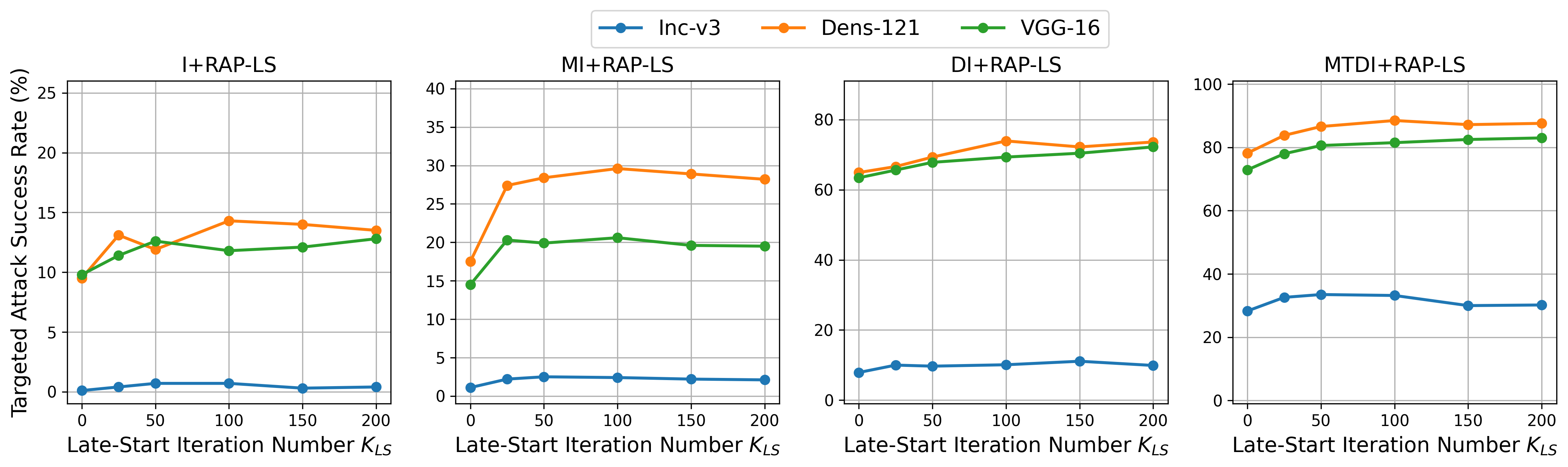
Figure 5: Targeted attack success rate ($\%$) with various $K_{LS}$. Res-50 is set as surrogate model.

4.7 The Targeted Attack Against Google Cloud Vision API

Finally, we conduct the transfer attacks to attack a practical and widely used image recognition system, Google Cloud Vision API, and in the more challenging targeted attack scenario. MTDAI-RAP-LS behaves the best performance in above experiments, so we choose it to conduct the attack. We take the evaluation on randomly selected 500 images and use ResNet-50 as surrogate model. As the API returns 10 predicted labels for each query, to evaluate the attacking performance, we test whether or not the target class appears in the returned predictions. Since the predicted label space of Google Cloud Vision API do not fully correspond to the 1000 ImageNet classes, we manually treat classes with similar semantics to be the same classes. In comparison, the baseline MTDAI successfully attacks $232$ images against the Google API. Our RAP-LS achieves a large improvement, successfully attacking $342$ images, leading to a 22.0% performance improvements. These demonstrates the high efficacy of our method to improve transferability on real-world system.

5 Conclusion

In this work, we study the transferability of adversarial examples that is significant for black-box attacks. The transferability of adversarial examples is generally influenced by the overfitting of surrogate models. To alleviate this, we propose to seeking adversarial examples that locate at flatter local regions. That is, instead of optimizing the pinpoint attack loss, we aim to obtain a consistently low loss at the neighbor regions of the adversarial examples. We formulate this as a min-max bi-level optimization problem, where the inner maximization aims to inject the worse-case perturbation for the adversarial examples. We conduct a rigorous experimental study, covering untargeted attack and targeted attack, standard and defense models, and a real-world Google Clould Vision API. The experimental results demonstrate that RAP can significantly boost the transferability of adversarial examples, which also demonstrates that transfer attacks have become serious threats. We need to consider how to effectively defense against them.

Acknowledgments

We want to thank the anonymous reviewers for their valuable suggestions and comments. This work is supported by the National Natural Science Foundation of China under grant No.62076213, Shenzhen Science and Technology Program under grant No.RCYX20210609103057050, and the university development fund of the Chinese University of Hong Kong, Shenzhen under grant No.01001810, and sponsored by CCF-Tencent Open Fund.

Appendix A Social Impact

Deep neural networks (DNNs) have been successfully applied in many safety-critical tasks, such as autonomous driving, face recognition and verification, etc. And adversarial samples have posed a serious threat to machine learning systems. For real-world applications, the DNN model as well as the training dataset, are often hidden from users. Therefore, the attackers need to generate the adversarial examples under black-box setting where they do not know any information of the target model. For black-box setting, the adversarial transferability matters since it can allow the attackers to attack target models by using adversarial examples generated on the surrogate models. This work can potentially contribute to understanding of transferability of adversarial examples. Besides, the better transferability of adversarial examples calls the machine learning and security communities into action to create stronger defenses and robust models against black-box attacks.

Appendix B Implementation Details

We conducted all experiments in an Nvidia-V100 GPU. And we run all experiments $3$ times and average all results over $3$ random seeds.

Dataset

The used two datasets are licensed under MIT. Imagenet is licensed under Custom (non-commercial).

Implementation Details of Evaluated Models.

For ResNet-50, DenseNet-121, VGG-16, Inception-v3, we adopt the pre-trained models provided by torchvision package. For Inception-ResNet-v2, NASNet-Large, ViT-Base/16, adv-Inc-v3, and ens-adv-Inc-Res-v2, we adopt the provided pre-trained models.

Implementation Details of Baseline Attack Methods.

We adopt the source code provided by Zhao et al. [49] to implement I, MI, TI, and DI attacks. The decay factor for MI is set as $1.0$. The kernel size is set as $5$ for TI attack, following Gao et al. [11]. The transformation probability is set as $0.7$ for DI. For SI and Admix, we adopt the parameters suggested in Wang et al. [41]. The number of copies for SI is set as $5$. The number of randomly sample $m_{2}$ and $\eta$ of Admix are set as $3$ and $0.2$ respectively. For implementation of ILA and LinBP, we utilize the source code provided by Guo et al. [14]. For implementation of TTP, we use the pre-trained generator based on ResNet-50 provided by [30].

Computational Cost.

Here, we analyze the computational cost of our method. In Algorithm 1 with global iteration number $K$, late-start iteration number $K_{LS}$ and inner iteration number $T$, our RAP-LS requires $K+\left(K-K_{LS}\right)*T$ forward and backward calculation. While the original attack algorithm requires $K$ forward and backward calculation. The extra computation cost of RAP-LS is $\left(K-K_{LS}\right)*T$ times forward and backward calculation.

The adversarial example generation process is conducted based on the offline surrogate models. Compared with this offline time cost, the attacking performance is much more important for black-box attacks. Besides, our late-start strategy could alleviate the time cost.

Implementation Details of Visualization.

We visualize the flatness of the loss landscape around $\bm{x}^{adv}$ on surrogate model by plotting the loss change when moving $\bm{x}^{adv}$ along a random direction with different magnitudes. Specially, we first sample $\bm{d}$ from a Gaussian distribution and normalize it on a $\ell_{2}$ unit norm ball, $\bm{d}\leftarrow\frac{\bm{d}}{\|\bm{d}\|_{F}}$. Then, we calculate the loss change (flatness) $f(a)$ with different magnitudes $a$,

$$f(a)=\mathcal{L}(\mathcal{M}^{s}(\mathcal{G}(\bm{x}^{adv}+a\cdot\bm{d});\bm{\theta}),y_{t})-\mathcal{L}(\mathcal{M}^{s}(\mathcal{G}(\bm{x}^{adv});\bm{\theta}),y_{t}).$$ (6)

Considering $\bm{d}$ is randomly selected, we repeat the above calculation 20 times with different $\bm{d}$ and take the averaged value to conduct the visualization.

We also add the visualization results about targeted attacks.

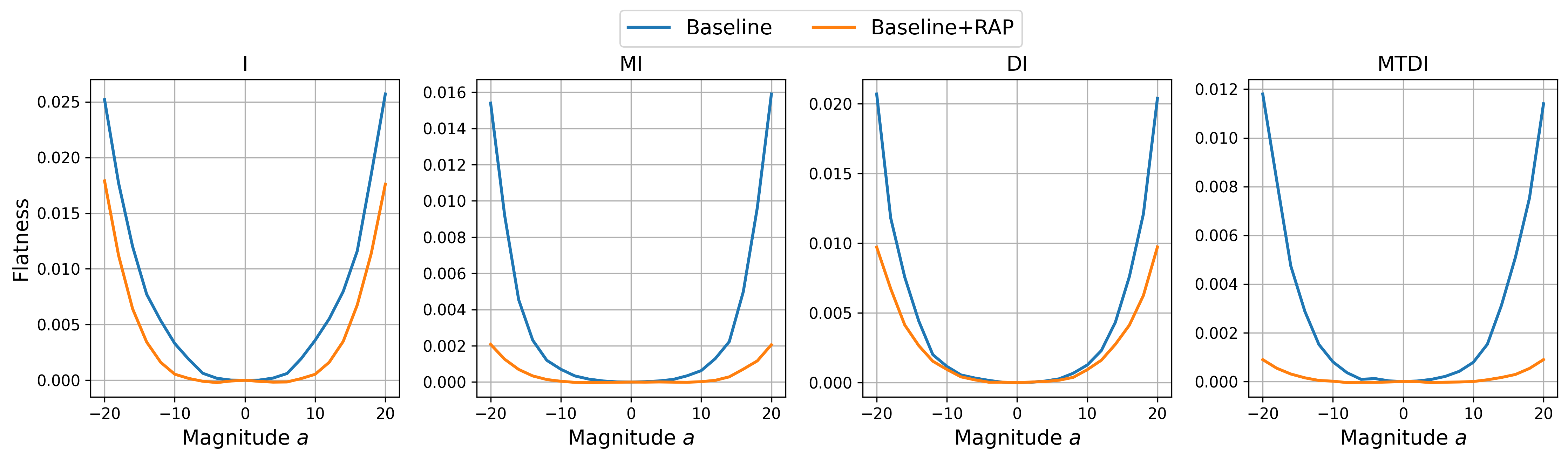
Figure 6: The flatness visualization of targeted adversarial examples.

Appendix C Experimental Results about More baseline attacks

In this section, we show the comparison of our method RAP and EOT [1], VT [40], EMI [42], and Ghost Net [22] attack methods.

C.1 Experimental Results about VT and EMI

In the below Table 8 and 9, we demonstrate the untargeted and targeted attack performance of VT, EMI, and our methods. We choose MI-TI-DI as the baseline method and follow experimental settings in Section 4.1. As shown in experimental results, our RAP-LS achieves better performance, especially for targeted attacks. Compared with VT, RAP-LS gets an increase of $6.7\%$ for targeted attacks in terms of average success rate. This demonstrates the effectiveness of our methods.

Table 8: The untargeted attack success rate ($\%$) of VT, EMI, and RAP-LS with the MI-TI-DI baseline.

Attack		ResNet-50 $\Longrightarrow$			DenseNet-121$\Longrightarrow$
	Dense-121	VGG-16	Inc-v3	Res-50	VGG-16	Inc-v3
MI-TI-DI	99.8	99.8	85.7	99.4	99.2	89.1
MI-TI-DI-VT	100	100	95.8	100	100	96.0
EMI-TI-DI	100	100	93.6	100	100	94.2
MI-TI-DI+RAP-LS	100	100	96.9	100	100	97.1
Attack		VGG-16 $\Longrightarrow$			Inc-v3$\Longrightarrow$
	Res-50	Dense-121	Inc-v3	Res-50	Dense-121	VGG-16
MI-TI-DI	90	88.8	56.8	82.9	85.7	85.1
MI-TI-DI-VT	93.9	93	76.5	87.1	90.3	87.5
EMI-TI-DI	91.7	91.5	74.3	86	88.4	86.2
MI-TI-DI+RAP-LS	97.7	97.3	81.4	90.6	93.3	91.0

Table 9: The targeted attack success rate ($\%$) of VT, EMI, and RAP-LS with the MI-TI-DI baseline

.

Attack		ResNet-50 $\Longrightarrow$			DenseNet-121$\Longrightarrow$
	Dense-121	VGG-16	Inc-v3	Res-50	VGG-16	Inc-v3
MI-TI-DI	74.9	62.8	10.9	44.9	38.5	7.7
MI-TI-DI-VT	82.5	71.9	21.6	59.2	53.6	21.3
EMI-TI-DI	79.1	67.8	19.2	56.3	50.4	19.8
MI-TI-DI+RAP-LS	88.5	81.5	33.2	74.5	65.5	26.5
Attack		VGG-16 $\Longrightarrow$			Inc-v3$\Longrightarrow$
	Res-50	Dense-121	Inc-v3	Res-50	Dense-121	VGG-16
MI-TI-DI	11.8	13.7	0.7	1.8	4.1	2.9
MI-TI-DI-VT	19.3	22.5	2.5	5.6	9.8	6.4
EMI-TI-DI	14.1	19.7	2.0	4.3	8.0	5.2
MI-TI-DI+RAP-LS	22.9	27.4	4.6	7.5	13.4	9.8

C.2 Experimental Results about Ghost Net attack

For combining Ghost net with RAP, we conduct the experiments on our PyTorch codes following the original TensorFlow codes provided by the authors. The main idea of ghost network is to perturb skip connections of ResNet to generate ensemble networks. To achieve this goal, the authors multiply skip connection by the random scalar $r$ sampled from a uniform distribution. We reimplement this procedure with the hyperparameter about $r$ recommended in the orginal paper on the PyTorch ResNet-50 model.

The targeted attack results ($\%$) are shown in the below Table 10. We also follow the experimental settings in Section 4.1. Here, we use GN to represent Ghost Net method. The results show that ghost network method can improve the transfer attack performance. Combined with RAP-LS, the adversarial transferability can be further improved especially on the inception-v3 model.

Table 10: The targeted attack success rate ($\%$) of GN, and RAP-LS with the MI-TI-DI baseline

Attack	ResNet-50 $\Longrightarrow$
	Dense-121	VGG-16	Inc-v3
MTDI	74.9	62.8	10.9
MTDI-GN	85.9	80.7	24.9
MTDI-GN+RAP-LS	89.6	87.7	49.7

C.3 Experimental Results about EOT attack

We conducted the experiment of the EOT baseline. We choose the ResNet-50 as the source model and MI-TI-DI as the baseline method. Instead of adding input transformation once like DI, we sample random transformation (resizing and padding) multiple times in each iteration. Then, we add them to following the expectation of transformation (EOT) [1]. We set the number of sampling as 10. Our RAP can be also naturally combined with EOT attack.

The targeted attack results ($\%$) are shown in the below Table 11. We also follow the experimental settings in Section 4.1.

As shown in the below table, 1) the EOT attack gets a moderate increase on attack performance compared with the baseline MI-TI-DI attack, which demonstrates that EOT could improve adversarial transferability. 2) Our RAP attack achieves better performance and surpasses the EOT attack by a large margin, especially for Inc-v3 and VGG-16 target models. 3) Combining RAP with EOT can further boost EOT attack performance. These results demonstrate that RAP could achieve better adversarial transferability and help find better flat local minima. Besides, the combination of RAP and EOT achieves the best performance among them, which demonstrates that these two methods could complement each other.

Table 11: The targeted attack success rate ($\%$) of EOT, and RAP-LS with the MI-TI-DI baseline

Attack	ResNet-50 $\Longrightarrow$
	Dense-121	VGG-16	Inc-v3
MTDI	74.9	62.8	10.9
MTDI-EOT	76.9	66.9	11.2
MTDI+RAP	78.2	72.9	28.3
MTDI-EOT+RAP	86.1	79.5	32.8

Appendix D Experimental Results about More Defense Models

The Evaluation on More Defense Models

Here, we show the evaluation of more defense models containing multi-step Adversarial training models in ImageNet [33], Feature Denoising [47], NRP [29], input transformation defense (R$\&$P) [46].

For Feature Denoising, we utilize the pre-trained ResNet-152 model provided by the authors . For AT models on ImageNet, we adopt the pre-trained ResNet-50 AT models provided by the authors . For $\ell_{\infty}$ norm, we adopt the ResNet-50 AT model with budget $4/255$, which ranks first in the RobustBench leaderboard . For $\ell_{2}$ norm, we adopt the ResNet-50 AT model with budget $0.5$. The untargeted attack performance is shown in Table 12. We follow the experimental settings in Section 4.5 of the main submission. We can observe that our RAP-LS further boosts the transferability of baseline methods on these new defense models, getting a $5.5\%$ boost for the average attack success rate.

For NRP, we adopt the pre-trained purifiers provided by the authors . Since NRP is an offline defense module, we combine it with the two used ensemble AT models and the above two AT models. The untargeted attack performance is shown in Table 13. We also follow the experimental settings in Section 4.5 of the main submission. Combining NRP with AT models is a much stronger defense mechanism, but RAP-LS still achieves an improvement by $0.8\%$.

For R$\&$P, we adopt the source code provided by [7] to implement it. We also combine R$\&$P with the two used ensemble AT models and the two new AT models above. The untargeted attack performance is shown in Table 14. We also follow the experimental settings in Section 4.5 of the main submission. For R$\&$P, RAP-LS achieves an $9.1\%$ increase in terms of average attack success rate.

Table 12: The evaluation of ensemble attacks on two AT models and Feature Noising.

Attack	Untarged
	Res-50 AT ($\ell_{2}$)	Res-50 AT ($\ell_{\infty}$)	Feature Denoising
MTDI	42.5	32.4	44.1
MTDI+RAP-LS	59.5	34.4	44.4
MTDSI	56.6	35.8	45.0
MTDSI+RAP-LS	70.3	36.6	45.7
MTDAI	62.1	35.6	44.2
MTDAI+RAP-LS	73.7	37.7	45.2

Table 13: The evaluation of ensemble attacks on defense models with NRP.

Attack	Untarged
	Inc-v3adv	IncRes-v2ens	Res-50 AT ($\ell_{2}$)	Res-50 AT ($\ell_{\infty}$)
MTDI	23.1	13.5	14.2	25.7
MTDI+RAP-LS	22.7	14.8	14.9	26.3
MTDSI	22.5	14.2	15.0	26.1
MTDSI+RAP-LS	24.5	15.3	15.4	26.2
MTDAI	24.1	14.7	14.2	25.9
MTDAI+RAP-LS	24.9	15.6	15.3	26.1

Table 14: The evaluation of ensemble attacks on defense models with R&P.

Attack	Untarged
	Inc-v3adv	IncRes-v2ens	Res-50 AT ($\ell_{2}$)	Res-50 AT ($\ell_{\infty}$)
MTDI	65.0	46.2	52.5	43.7
MTDI+RAP-LS	82.1	63.2	65.3	45.8
MTDSI	86.5	69.6	64.1	45.9
MTDSI+RAP-LS	93.4	84.9	74.0	46.2
MTDAI	88.9	76.5	68.4	46.2
MTDAI+RAP-LS	94.8	87.0	77.7	47.7

The above experimental results also show that RAP is less effective when attacking Feature Denoising. We think this is mainly due to the specially designed feature denoising block (i.e. the non-local block), and the different settings of maximum perturbation size during adversarial training, as follows.

• Feature Denoising [47] inserts several non-local blocks into network to eliminate the adversarial noise at the feature level. According to [47], for input feature map $F_{i}$, the non-local block computes a denoised output feature map $F_{0}$ by taking a weighted average of input features in all spatial locations. Through this, the non-local block would model the global relationship between features in all spatial locations, which may smooth the learned decision boundary. Recalling that our RAP is to boost the transferability by seeking for a flat local minimum. The smoothness of decision boundary could make it harder to escape from certain local minimum, especially for small attack perturbation size, so as to limit the performance improvement of RAP.

• In our experiment, for Feature Denoising, the maximum perturbation size during their training is set to 16/255. In Table 12, the maximum perturbation size of attack is also set to 16/255. The attack size of 16/255 may not be large enough for escaping from local minima for the Feature Denoising model trained with 16/255 perturbation size. In contrast, the maximum perturbation size of AT-$\ell_{\infty}$ during training is 4/255. To verify this, we conduct an ablation study of increasing the maximum perturbation size to 20/255. Using a larger perturbation size of 20/255, the attacking performance against Feature Denoising is $48.3\%$ for MI-TI-DI and $50.7\%$ for MI-TI-DI+RAP-LS. The relative performance improvement of RAP-LS is $2.4\%$, which is much larger than the relative performance improvement of $0.3\%$ in Table 12 with perturbation size 16/255, which may partially explain the phenomenon.

Appendix E Additional Experimental Results

In this section, we first show the evaluation of targeted attacks with CE loss in Section E.1. Then we show the results of ensemble attacks on more diverse network architectures in Section E.2. In Section E.3, we report the experimental results w.r.t. different value of iterations.

E.1 The Results of Targeted Attacks with CE Loss

Following the settings in main submission, we evaluate the targeted attack performance of the different baseline methods with our method on ResNet-50, DenseNet-121, VGG-16, and Inception-v3. The results of combinational methods are shown in Table 15. The RAP-LS outperforms all combinational methods by a significantly margin. Taking the average attack success rate of all target models as the evaluation metric, RAP-LS achieves $20.9\%$, $18.4\%$, and $15.1\%$ improvements over the MTDI, MTDSI and MTDAI, respectively.

Table 15: The targeted attack success rate ($\%$) of combinational methods with RAP. The results with $CE$ loss and 400 iterations are reported. The best results are bold and the second best results are underlined.

Attack		ResNet-50 $\Longrightarrow$			DenseNet-121$\Longrightarrow$
	Dense-121	VGG-16	Inc-v3	Res-50	VGG-16	Inc-v3
MTDI / +RAP / +RAP-LS	45.5 / 78.3 / 85.9	29.8 / 70.5 / 76.7	4.5 / 21.3 / 25.3	20.0 / 54.0 / 62.7	9.9 / 41.7 / 48.7	2.6 / 17.5 / 18.5
MTDSI / +RAP / +RAP-LS	77.7 / 89.0 / 93.7	39.9 / 69.4 / 76.7	26.9 / 45.3 / 50.8	30.5 / 60.4 / 69.5	14.9 / 42.8 / 49.7	12.7 / 26.6 / 32.5
MTDAI / +RAP / +RAP-LS	90.2 / 91.4 / 96.1	61.8 / 73.7 / 83.4	44.5 / 47.9 / 59.0	55.8 / 68.4 / 79.3	35.1 / 51.8 / 64.1	26.3 / 32.4 / 40.4
Attack		VGG-16 $\Longrightarrow$			Inc-v3$\Longrightarrow$
	Res-50	Dense-121	Inc-v3	Res-50	Dense-121	VGG-16
MTDI / +RAP / +RAP-LS	0.5 / 10.4 / 12.1	0.1 / 11.0 / 13.5	0.0 / 1.7 / 2.0	2.2 / 4.9 / 5.9	2.2 / 9.8 / 11.0	1.2 / 4.9 / 6.7
MTDSI / +RAP / +RAP-LS	5.4 / 17.4 / 16.8	9.5 / 28.4 / 25.2	2.2 / 7.1 / 5.1	4.4 / 8.6 / 8.9	7.9 / 16.3 / 19.3	2.0 / 6.4 / 6.4
MTDAI / +RAP / +RAP-LS	11.6 / 22.6 / 26.6	20.6 / 32.1 / 39.1	5.1 / 9.2 / 9.5	6.7 / 12.3 / 17.0	14.0 / 22.9 / 29.2	4.5 / 9.4 / 13.2

E.2 The Results of Ensemble Attacks on Diverse Network Architectures

We also take the evaluation of the ensemble attacks on diverse network architecture (Sec.4.5). We adopt the ensemble-model attack by averaging the logits of different surrogate models, including ResNet-50, DenseNet-121, VGG-16, and Inception-v3. The transfer attack success rate on diverse models are shown in Table 16. Compared with results of single model attack in Table 7, the ensemble attack achieve the better performance. We can observe that our RAP-LS further boosts transferability of the baseline methods on both targeted and untargeted attacks. We take ViT as target model for example. For untargeted attacks, RAP-LS achieves average performance improvements of $19.2\%$. For targeted attacks, RAP-LS achieves average performance improvements of $10.4\%$.

Table 16: The evaluation of ensemble attacks on diverse network architectures.

Attack	Untarged			Targeted
	IncRes-v2	NASNet-L	ViT-B/16	IncRes-v2	NASNet-L	ViT-B/16
MTDI	98.6	99.3	46.2	65.7	80.1	2.8
MTDI+RAP-LS	100	100	73.2	84.4	89.7	12.7
MTDSI	99.8	100	68.3	81.7	89.4	15.0
MTDSI+RAP-LS	100	100	85.0	89.8	92.3	25.1
MTDAI	100	100	70.7	88.8	91.2	16.8
MTDAI+RAP-LS	100	100	84.6	90.4	91.8	27.8

E.3 The Experimental Results w.r.t Different Value of Iterations

In the main submission, we report the evaluations of $K=400$. Here, we further report the performance with different values of $K$ for completeness in Table 17 (targeted attack) and Table 18 (untargeted attack). From the results, we observe that the attacking performance generally increase as $K$ increases for most cases, this is also aligned with prior works [49].

Table 17: The targeted attack success rate ($\%$) of all baseline attacks with our method. The results with logit loss and 10/100/200/300/400 iterations are reported. We highlight the results with $K=400$ in bold.

	ResNet-50 $\bm{\rightarrow}$ Inception-v3
	Baseline	+RAP	+RAP-LS
I	0.0 / 0.1 / 0.2 / 0.1 / 0.1	0.0 / 0.2 / 0.3 / 0.3 / 0.1	0.0 / 0.1 / 0.4 / 0.6 / 0.7
MI	0.1 / 0.1 / 0.2 / 0.1 / 0.1	0.0 / 0.6 / 1.0 / 1.0 / 1.1	0.1 / 0.1 / 1.4 / 1.6 / 2.4
TI	0.0 / 0.3 / 0.2 / 0.2 / 0.1	0.0 / 0.7 / 0.9 / 1.2 / 0.8	0.0 / 0.3 / 1.3 / 1.3 / 1.2
DI	0.2 / 1.2 / 1.7 / 1.5 / 1.5	0.0 / 3.8 / 6.6 / 7.7 / 7.9	0.2 / 1.2 / 10.2 / 9.4 / 10.1
SI	0.3 / 2.6 / 2.4 / 2.0 / 1.8	0.2 / 6.6 / 8.2 / 8.6 / 9.3	0.3 / 2.6 / 9.6 / 9.3 / 10.5
Admix	1.4 / 5.7 / 5.9 / 6.0 / 5.8	0.6 / 14.6 / 16.6 / 16.5 / 17.1	1.4 / 5.7 / 18.5 / 19.2 / 19.6
MI-TI-DI	1.5 / 7.9 / 9.8 / 10.5 / 10.9	0.1 / 12.7 / 22.3 / 26.3 / 28.3	1.5 / 7.9 / 26.8 / 30.0 / 33.2
MI-TI-DI-SI	8.9 / 34.1 / 36.7 / 38.1 / 38.1	3.3 / 43.3 / 47.9 / 49.9 / 51.8	8.9 / 34.8 / 54.8 / 55.8 / 58.0
MI-TI-DI-Admix	13.5 / 45.7 / 49.2 / 50.5 / 50.8	5.0 / 48.1 / 53.4 / 56.2 / 57.1	13.5 / 45.1 / 61.4 / 63.0 / 64.1

	ResNet-50 $\bm{\rightarrow}$ DenseNet-121
	Baseline	+RAP	+RAP-LS
I	0.9 / 5.3 / 5.0 / 5.5 / 4.5	0.0 / 4.8 / 7.9 / 8.8 / 9.5	0.9 / 5.3 / 14.0 / 14.0 / 14.3
MI	3.4 / 6.3 / 6.3 / 6.0 / 6.3	0.2 / 9.0 / 14.1 / 15.8 / 17.5	3.4 / 6.3 / 25.9 / 28.9 / 29.6
TI	2.5 / 8.6 / 8.9 / 9.0 / 7.2	0.0 / 7.1 / 10.1 / 11.2 / 11.0	2.5 / 8.6 / 16.1 / 16.4 / 17.3
DI	8.4 / 54.8 / 60.4 / 61.2 / 62.6	0.1 / 40.6 / 53.2 / 59.4 / 64.9	8.4 / 54.6 / 70.9 / 72.5 / 73.9
SI	9.7 / 29.6 / 30.4 / 30.4 / 30.0	2.2 / 45.8 / 50.9 / 52.5 / 53.2	9.7 / 29.6 / 60.0 / 61.1 / 61.1
Admix	23.6 / 55.6 / 55.5 / 55.6 / 54.6	5.3 / 61.2 / 66.0 / 66.9 / 68.0	23.6 / 55.6 / 74.4 / 74.7 / 74.6
MI-TI-DI	16.3 / 66.9 / 71.4 / 73.4 / 74.9	1.8 / 56.7 / 71.2 / 76.4 / 78.2	16.3 / 66.7 / 85.2 / 85.7 / 88.5
MI-TI-DI-SI	41.0 / 82.8 / 84.5 / 86.2 / 86.3	12.9 / 80.2 / 85.7 / 87.8 / 88.4	41.0 / 82.5 / 91.9 / 92.4 / 93.3
MI-TI-DI-Admix	48.0 / 88.7 / 90.9 / 91.1 / 91.4	20.3 / 83.2 / 87.2 / 88.4 / 89.4	47.9 / 88.5 / 93.5 / 93.8 / 93.6

	ResNet-50 $\bm{\rightarrow}$ VGG-16
	Baseline	+RAP	+RAP-LS
I	1.0 / 2.7 / 2.6 / 2.3 / 2.4	0.0 / 5.6 / 8.3 / 9.8 / 9.8	1.0 / 2.7 / 11.4 / 12.8 / 11.8
MI	1.2 / 2.1 / 2.4 / 2.2 / 2.2	0.1 / 8.6 / 12.3 / 14.1 / 14.5	1.2 / 2.1 / 18.2 / 20.0 / 20.6
TI	1.1 / 4.8 / 4.8 / 4.5 / 4.0	0.1 / 6.0 / 9.3 / 9.9 / 12.9	1.1 / 4.8 / 14.2 / 15.3 / 15.3
DI	7.6 / 51.0 / 56.9 / 56.6 / 57.2	0.4 / 42.4 / 55.0 / 61.5 / 63.4	7.6 / 51.0 / 69.3 / 69.8 / 69.3
SI	4.4 / 10.4 / 8.9 / 8.8 / 9.5	1.1 / 27.8 / 31.1 / 30.7 / 32.8	4.4 / 10.4 / 35.8 / 35.1 / 36.0
Admix	10.6 / 24.9 / 25.0 / 26.2 / 26.0	3.6 / 41.4 / 45.2 / 43.8 / 45.4	10.6 / 24.9 / 51.7 / 51.9 / 51.6
MI-TI-DI	12.1 / 55.9 / 61.0 / 63.9 / 62.8	1.5 / 53.0 / 64.7 / 70.9 / 72.9	12.1 / 55.8 / 78.5 / 81.7 / 81.5
MI-TI-DI-SI	24.6 / 67.4 / 68.5 / 69.7 / 70.1	8.2 / 66.4 / 73.7 / 75.2 / 77.7	24.5 / 66.4 / 82.4 / 83.7 / 84.7
MI-TI-DI-Admix	33.4 / 75.3 / 77.5 / 78.7 / 79.9	14.6 / 70.4 / 76.7 / 78.3 / 79.0	33.3 / 75.2 / 85.4 / 86.4 / 86.3

	DenseNet121 $\bm{\rightarrow}$ Inception-v3
	Baseline	+RAP	+RAP-LS
I	0.0 / 0.1 / 0.2 / 0.1 / 0.0	0.0 / 0.6 / 0.9 / 0.7 / 0.8	0.0 / 0.1 / 1.0 / 1.3 / 1.2
MI	0.2 / 0.2 / 0.3 / 0.3 / 0.3	0.0 / 1.2 / 2.1 / 2.1 / 2.0	0.2 / 0.2 / 2.5 / 3.7 / 3.4
TI	0.0 / 0.4 / 0.3 / 0.5 / 0.2	0.0 / 1.2 / 1.5 / 1.6 / 2.1	0.0 / 0.4 / 2.6 / 3.1 / 3.0
DI	0.3 / 1.9 / 1.4 / 1.7 / 1.4	0.0 / 4.1 / 7.0 / 7.6 / 8.8	0.3 / 1.9 / 9.3 / 9.9 / 10.0
SI	0.3 / 1.5 / 1.8 / 1.6 / 1.6	0.1 / 7.6 / 9.2 / 10.0 / 8.5	0.3 / 1.5 / 9.2 / 10.7 / 10.4
Admix	1.7 / 5.0 / 5.4 / 5.5 / 5.0	0.2 / 15.8 / 17.0 / 17.7 / 17.1	1.7 / 5.0 / 18.5 / 18.2 / 17.6
MI-TI-DI	1.2 / 6.8 / 7.9 / 8.7 / 7.7	0.1 / 13.0 / 19.7 / 22.2 / 23.0	1.2 / 6.7 / 21.9 / 26.2 / 26.5
MI-TI-DI-SI	5.1 / 17.6 / 18.9 / 19.3 / 19.8	2.0 / 30.4 / 35.1 / 37.0 / 39.0	5.2 / 17.7 / 36.8 / 38.9 / 39.2
MI-TI-DI-Admix	11.4 / 30.5 / 32.2 / 31.4 / 32.0	3.9 / 36.7 / 41.3 / 42.2 / 43.5	11.2 / 31.2 / 47.2 / 49.2 / 49.3

	DenseNet121 $\bm{\rightarrow}$ ResNet-50
	Baseline	+RAP	+RAP-LS
I	1.8 / 6.5 / 5.6 / 5.5 / 5.0	0.2 / 7.7 / 11.2 / 12.4 / 12.8	1.8 / 6.5 / 18.7 / 19.0 / 17.9
MI	3.4 / 5.4 / 5.2 / 4.9 / 4.6	0.3 / 10.2 / 14.3 / 16.3 / 16.2	3.4 / 5.4 / 23.6 / 26.3 / 26.5
TI	2.6 / 8.1 / 7.9 / 8.4 / 8.4	0.2 / 7.8 / 10.9 / 12.1 / 13.5	2.6 / 8.1 / 19.2 / 20.2 / 20.8
DI	6.3 / 30.4 / 33.1 / 32.0 / 30.2	0.4 / 33.6 / 44.1 / 48.7 / 52.6	6.3 / 30.8 / 58.8 / 60.4 / 60.4
SI	7.3 / 16.5 / 15.9 / 14.8 / 14.2	1.5 / 33.8 / 39.5 / 41.4 / 41.5	7.3 / 16.5 / 44.7 / 44.8 / 43.4
Admix	16.4 / 32.6 / 30.3 / 28.8 / 29.3	3.7 / 48.3 / 52.9 / 53.4 / 53.0	16.4 / 32.6 / 60.1 / 58.8 / 58.2
MI-TI-DI	8.3 / 40.3 / 44.6 / 46.3 / 44.9	0.9 / 42.0 / 56.4 / 62.4 / 64.3	8.3 / 40.1 / 69.5 / 72.8 / 74.5
MI-TI-DI-SI	18.6 / 52.3 / 54.1 / 56.2 / 55.0	6.6 / 60.3 / 67.5 / 70.6 / 71.2	18.6 / 52.5 / 73.8 / 75.5 / 75.8
MI-TI-DI-Admix	27.6 / 66.3 / 69.7 / 69.8 / 69.1	12.1 / 66.4 / 70.8 / 73.2 / 74.2	27.6 / 66.4 / 81.4 / 82.0 / 82.1

	DenseNet121 $\bm{\rightarrow}$ VGG-16
	Baseline	+RAP	+RAP-LS
I	0.6 / 3.8 / 3.5 / 3.5 / 2.9	0.1 / 6.2 / 9.3 / 10.5 / 10.1	0.6 / 3.8 / 14.5 / 15.7 / 15.9
MI	1.6 / 2.4 / 2.6 / 2.7 / 3.1	0.2 / 8.6 / 12.2 / 13.0 / 13.4	1.6 / 2.4 / 19.5 / 21.7 / 23.2
TI	1.1 / 5.6 / 5.8 / 4.8 / 5.2	0.1 / 6.3 / 9.1 / 11.0 / 12.4	1.1 / 5.6 / 16.5 / 17.0 / 16.4
DI	4.1 / 29.8 / 32.7 / 33.1 / 32.1	0.2 / 31.5 / 44.7 / 48.7 / 49.5	4.1 / 29.9 / 57.2 / 56.5 / 58.9
SI	2.8 / 9.8 / 8.8 / 8.5 / 8.4	0.6 / 25.8 / 28.2 / 31.4 / 31.0	2.8 / 9.8 / 33.5 / 35.3 / 35.2
Admix	10.2 / 23.3 / 22.1 / 21.3 / 21.5	1.7 / 39.4 / 42.2 / 43.0 / 42.7	10.2 / 23.3 / 49.7 / 49.3 / 48.2
MI-TI-DI	6.1 / 32.4 / 36.3 / 39.0 / 38.5	0.7 / 36.2 / 49.9 / 53.2 / 55.0	6.1 / 32.6 / 61.8 / 64.3 / 65.5
MI-TI-DI-SI	12.4 / 40.2 / 41.9 / 42.2 / 42.0	4.6 / 46.9 / 54.0 / 57.0 / 58.4	12.4 / 40.0 / 61.3 / 62.4 / 62.3
MI-TI-DI-Admix	20.0 / 53.2 / 55.0 / 55.7 / 54.7	9.4 / 54.8 / 60.1 / 61.8 / 63.1	19.9 / 53.1 / 68.1 / 69.7 / 69.3

	VGG-16 $\bm{\rightarrow}$ Inception-v3
	Baseline	+RAP	+RAP-LS
I	0.0 / 0.0 / 0.0 / 0.0 / 0.0	0.0 / 0.1 / 0.0 / 0.1 / 0.1	0.0 / 0.0 / 0.2 / 0.0 / 0.2
MI	0.0 / 0.0 / 0.0 / 0.0 / 0.0	0.0 / 0.0 / 0.2 / 0.0 / 0.0	0.0 / 0.0 / 0.2 / 0.5 / 0.3
TI	0.0 / 0.0 / 0.0 / 0.1 / 0.0	0.0 / 0.1 / 0.1 / 0.1 / 0.1	0.0 / 0.0 / 0.4 / 0.4 / 0.4
DI	0.0 / 0.0 / 0.0 / 0.0 / 0.0	0.0 / 0.0 / 0.4 / 0.6 / 0.4	0.0 / 0.0 / 0.7 / 0.7 / 1.1
SI	0.0 / 0.4 / 0.3 / 0.2 / 0.2	0.0 / 2.0 / 1.5 / 2.0 / 1.7	0.0 / 0.6 / 1.6 / 1.9 / 1.8
Admix	0.1 / 0.7 / 0.8 / 0.6 / 0.7	0.0 / 2.7 / 2.2 / 2.3 / 2.4	0.1 / 1.0 / 2.3 / 3.0 / 2.8
MI-TI-DI	0.1 / 1.0 / 0.8 / 1.1 / 0.7	0.0 / 1.8 / 2.8 / 3.0 / 3.4	0.1 / 0.9 / 3.4 / 4.0 / 4.6
MI-TI-DI-SI	1.7 / 7.7 / 9.1 / 9.8 / 9.6	0.6 / 12.2 / 14.5 / 13.8 / 15.2	1.7 / 8.6 / 11.4 / 12.1 / 13.7
MI-TI-DI-Admix	3.6 / 12.4 / 12.2 / 11.5 / 11.6	1.1 / 14.5 / 16.1 / 15.9 / 17.1	3.4 / 11.2 / 15.9 / 17.4 / 17.6

	VGG-16 $\bm{\rightarrow}$ ResNet-50
	Baseline	+RAP	+RAP-LS
I	0.2 / 0.4 / 0.3 / 0.3 / 0.1	0.0 / 1.0 / 0.8 / 0.8 / 0.7	0.2 / 0.5 / 1.4 / 1.5 / 1.4
MI	0.4 / 0.5 / 0.6 / 0.5 / 0.5	0.2 / 1.1 / 1.3 / 1.3 / 1.3	0.4 / 0.2 / 2.1 / 2.4 / 1.9
TI	0.3 / 1.0 / 0.7 / 0.9 / 0.7	0.0 / 1.4 / 1.5 / 1.4 / 1.2	0.3 / 1.0 / 3.0 / 3.3 / 3.2
DI	0.5 / 2.8 / 3.1 / 3.4 / 2.8	0.0 / 4.9 / 6.7 / 6.5 / 7.3	0.5 / 3.9 / 9.5 / 10.1 / 9.7
SI	1.4 / 4.4 / 3.9 / 3.8 / 3.3	0.4 / 9.2 / 9.0 / 9.1 / 9.8	1.4 / 4.3 / 10.1 / 9.4 / 9.8
Admix	4.6 / 7.3 / 6.7 / 5.8 / 5.6	0.7 / 10.6 / 11.3 / 10.9 / 11.1	4.7 / 7.3 / 11.6 / 12.5 / 11.9
MI-TI-DI	1.8 / 10.2 / 11.7 / 11.9 / 11.8	0.0 / 10.8 / 14.6 / 15.7 / 16.7	1.8 / 9.5 / 20.2 / 21.6 / 22.9
MI-TI-DI-SI	8.8 / 30.1 / 31.6 / 30.3 / 31.0	3.2 / 30.8 / 32.5 / 33.5 / 35.3	9.0 / 29.5 / 36.9 / 38.5 / 38.7
MI-TI-DI-Admix	15.2 / 34.6 / 35.1 / 36.6 / 36.2	5.4 / 34.7 / 37.3 / 38.1 / 39.0	15.3 / 35.5 / 43.2 / 42.9 / 43.1

	VGG-16 $\bm{\rightarrow}$ DenseNet-121
	Baseline	+RAP	+RAP-LS
I	0.1 / 0.2 / 0.4 / 0.3 / 0.2	0.0 / 0.7 / 1.1 / 0.7 / 1.4	0.1 / 0.3 / 1.2 / 1.5 / 1.7
MI	0.3 / 0.8 / 0.6 / 0.6 / 0.5	0.0 / 1.1 / 1.4 / 2.1 / 2.3	0.3 / 0.6 / 2.4 / 3.2 / 3.0
TI	0.1 / 0.6 / 1.1 / 1.0 / 0.8	0.0 / 0.9 / 1.7 / 1.6 / 1.7	0.1 / 0.9 / 2.5 / 2.7 / 2.9
DI	0.2 / 3.8 / 4.8 / 4.1 / 3.8	0.0 / 5.0 / 7.6 / 7.8 / 8.4	0.2 / 3.7 / 11.9 / 12.2 / 12.7
SI	1.3 / 9.0 / 8.9 / 7.7 / 7.2	0.3 / 14.0 / 15.6 / 16.4 / 16.8	1.3 / 8.2 / 17.0 / 17.4 / 17.8
Admix	4.9 / 14.3 / 13.4 / 13.2 / 13.0	0.7 / 17.9 / 20.5 / 20.2 / 20.2	4.9 / 14.0 / 23.9 / 24.2 / 23.6
MI-TI-DI	1.5 / 12.1 / 13.4 / 13.9 / 13.7	0.1 / 9.7 / 15.7 / 17.4 / 19.4	1.6 / 12.1 / 24.4 / 26.3 / 27.4
MI-TI-DI-SI	13.0 / 38.9 / 41.5 / 42.8 / 41.7	3.8 / 37.8 / 42.0 / 43.8 / 44.4	12.8 / 37.3 / 48.6 / 49.8 / 49.6
MI-TI-DI-Admix	19.0 / 45.5 / 47.0 / 47.7 / 48.0	6.8 / 41.3 / 45.2 / 44.8 / 45.1	19.1 / 45.3 / 52.9 / 54.9 / 55.2

	Inc-v3 $\bm{\rightarrow}$ ResNet-50
	Baseline	+RAP	+RAP-LS
I	0.2 / 0.4 / 0.3 / 0.1 / 0.2	0.0 / 0.2 / 0.7 / 0.6 / 0.9	0.2 / 0.4 / 1.0 / 0.7 / 0.5
MI	0.1 / 0.3 / 0.3 / 0.2 / 0.2	0.0 / 0.6 / 1.4 / 1.5 / 1.7	0.1 / 0.3 / 0.8 / 1.6 / 1.5
TI	0.2 / 0.3 / 0.2 / 0.2 / 0.2	0.0 / 0.2 / 0.6 / 0.9 / 0.5	0.2 / 0.3 / 1.0 / 0.7 / 0.7
DI	0.2 / 1.5 / 1.4 / 1.9 / 1.6	0.1 / 2.5 / 4.3 / 4.3 / 4.6	0.2 / 1.5 / 5.0 / 5.1 / 6.4
SI	0.3 / 0.3 / 0.3 / 0.6 / 0.6	0.4 / 1.9 / 2.6 / 2.6 / 2.9	0.3 / 0.3 / 2.4 / 2.8 / 2.5
Admix	1.2 / 1.9 / 2.2 / 1.9 / 1.5	0.6 / 5.0 / 4.9 / 5.2 / 4.9	1.2 / 1.9 / 5.7 / 5.7 / 5.2
MI-TI-DI	0.6 / 1.6 / 2.0 / 2.4 / 1.8	0.0 / 4.2 / 6.3 / 7.7 / 8.3	0.6 / 1.7 / 6.2 / 7.0 / 7.5
MI-TI-DI-SI	1.5 / 4.7 / 5.5 / 5.8 / 5.6	0.7 / 8.6 / 10.3 / 11.1 / 11.9	1.5 / 5.0 / 10.0 / 9.6 / 10.7
MI-TI-DI-Admix	2.8 / 8.9 / 9.5 / 9.6 / 9.6	1.4 / 12.6 / 14.0 / 13.6 / 13.6	2.8 / 8.6 / 14.5 / 15.1 / 16.7

	Inc-v3 $\bm{\rightarrow}$ DenseNet-121
	Baseline	+RAP	+RAP-LS
I	0.0 / 0.0 / 0.2 / 0.0 / 0.2	0.0 / 0.2 / 0.4 / 0.6 / 0.6	0.0 / 0.0 / 0.2 / 0.4 / 0.3
MI	0.0 / 0.1 / 0.2 / 0.1 / 0.1	0.1 / 0.7 / 1.0 / 1.1 / 1.6	0.0 / 0.1 / 1.0 / 1.1 / 1.5
TI	0.0 / 0.3 / 0.2 / 0.0 / 0.1	0.0 / 0.3 / 0.3 / 0.3 / 0.7	0.0 / 0.3 / 0.9 / 0.9 / 0.6
DI	0.1 / 1.3 / 2.5 / 3.0 / 2.8	0.0 / 2.7 / 4.4 / 5.4 / 5.8	0.1 / 1.3 / 5.9 / 7.0 / 7.5
SI	0.2 / 0.7 / 0.9 / 0.8 / 0.9	0.0 / 2.4 / 3.3 / 2.9 / 2.7	0.2 / 0.7 / 3.2 / 3.1 / 3.2
Admix	1.1 / 2.6 / 2.5 / 2.3 / 2.0	0.5 / 7.2 / 7.7 / 7.0 / 6.9	1.1 / 2.6 / 8.2 / 7.3 / 7.5
MI-TI-DI	0.5 / 3.1 / 3.8 / 4.5 / 4.1	0.2 / 5.4 / 10.8 / 12.6 / 14.8	0.5 / 3.3 / 10.6 / 11.8 / 13.4
MI-TI-DI-SI	1.9 / 9.0 / 9.4 / 9.5 / 10.4	1.1 / 15.5 / 19.8 / 19.8 / 21.2	1.9 / 9.0 / 19.1 / 20.2 / 20.9
MI-TI-DI-Admix	4.6 / 15.7 / 16.8 / 17.4 / 17.9	2.4 / 23.2 / 24.5 / 26.6 / 27.5	4.6 / 15.0 / 29.1 / 30.2 / 31.6

	Inc-v3 $\bm{\rightarrow}$ VGG-16
	Baseline	+RAP	+RAP-LS
I	0.0 / 0.3 / 0.1 / 0.1 / 0.1	0.0 / 0.2 / 0.8 / 0.6 / 0.5	0.0 / 0.3 / 0.2 / 0.5 / 0.5
MI	0.1 / 0.1 / 0.2 / 0.2 / 0.2	0.1 / 0.4 / 0.8 / 1.2 / 1.3	0.1 / 0.1 / 0.4 / 0.8 / 1.0
TI	0.1 / 0.2 / 0.2 / 0.1 / 0.2	0.1 / 0.4 / 0.5 / 0.6 / 0.8	0.1 / 0.2 / 0.6 / 0.6 / 0.6
DI	0.3 / 2.0 / 2.8 / 2.3 / 2.6	0.1 / 1.8 / 4.3 / 5.2 / 6.3	0.3 / 2.0 / 6.8 / 7.3 / 8.1
SI	0.0 / 0.7 / 0.6 / 0.4 / 0.5	0.2 / 2.0 / 1.5 / 1.5 / 1.5	0.0 / 0.7 / 1.6 / 2.3 / 2.3
Admix	0.5 / 1.6 / 1.0 / 1.0 / 1.3	0.4 / 3.2 / 3.8 / 4.1 / 3.3	0.5 / 1.6 / 4.5 / 3.8 / 4.4
MI-TI-DI	0.3 / 2.0 / 2.4 / 2.7 / 2.9	0.1 / 3.8 / 6.5 / 7.3 / 8.0	0.3 / 2.0 / 8.0 / 7.9 / 9.8
MI-TI-DI-SI	0.7 / 3.7 / 3.6 / 4.1 / 4.2	0.5 / 7.6 / 7.5 / 8.5 / 8.9	0.7 / 3.2 / 6.7 / 8.1 / 8.6
MI-TI-DI-Admix	2.3 / 6.9 / 8.3 / 8.6 / 8.4	1.3 / 10.5 / 12.5 / 12.0 / 12.0	2.3 / 7.0 / 11.9 / 12.8 / 12.1

Table 18: The untargeted attack success rate ($\%$) of all baseline attacks with RAP. The results with $CE$ loss and 10/100/200/300/400 iterations are reported. We highlight the results with $K=400$ in bold.

	ResNet-50 $\bm{\rightarrow}$ Inception-v3
	Baseline	+RAP	+RAP-LS
I	25.9 / 35.5 / 35.3 / 34.7 / 34.6	12.3 / 48.3 / 54.1 / 55.5 / 57.0	25.7 / 36.0 / 54.1 / 56.5 / 57.2
MI	53.2 / 50.7 / 51.0 / 50.6 / 50.3	26.2 / 58.7 / 68.9 / 73.4 / 75.9	53.2 / 50.7 / 64.3 / 73.6 / 77.4
TI	30.0 / 45.3 / 44.0 / 45.3 / 45.5	16.4 / 57.9 / 63.9 / 64.6 / 66.1	30.0 / 45.1 / 62.3 / 65.3 / 67.0
DI	46.0 / 60.5 / 59.5 / 59.4 / 57.7	27.3 / 80.7 / 82.8 / 83.4 / 82.9	46.0 / 61.0 / 86.0 / 85.7 / 85.0
SI	50.1 / 66.0 / 65.6 / 66.0 / 65.9	60.6 / 80.5 / 80.9 / 80.9 / 79.7	49.9 / 66.6 / 85.2 / 85.0 / 84.4
Admix	66.6 / 78.7 / 79.2 / 78.0 / 77.7	73.9 / 87.6 / 87.0 / 86.8 / 87.4	67.6 / 79.4 / 91.8 / 92.3 / 92.6
MI-TI-DI	82.1 / 85.8 / 86.4 / 85.9 / 85.7	61.9 / 93.9 / 95.3 / 95.6 / 96.0	82.1 / 85.8 / 95.9 / 96.4 / 96.9
MI-TI-DI-SI	94.2 / 96.8 / 97.2 / 97.0 / 97.0	92.3 / 98.9 / 98.9 / 99.0 / 99.1	94.2 / 96.7 / 99.0 / 99.3 / 99.1
MI-TI-DI-Admix	97.3 / 98.6 / 98.5 / 98.5 / 98.3	95.1 / 99.4 / 99.4 / 99.3 / 99.2	97.3 / 98.5 / 99.8 / 99.8 / 99.8

	ResNet-50 $\bm{\rightarrow}$ DenseNet-121
	Baseline	+RAP	+RAP-LS
I	67.4 / 79.9 / 79.1 / 79.0 / 79.2	26.7 / 84.8 / 91.1 / 90.8 / 91.5	67.8 / 80.1 / 89.8 / 91.3 / 91.9
MI	87.3 / 85.4 / 86.4 / 85.9 / 85.8	45.2 / 85.3 / 91.3 / 93.9 / 95.0	87.3 / 85.4 / 90.8 / 95.0 / 96.1
TI	73.2 / 83.0 / 82.2 / 81.6 / 82.0	30.9 / 87.3 / 91.5 / 93.3 / 94.1	72.9 / 82.4 / 90.9 / 94.2 / 95.1
DI	92.8 / 98.9 / 99.2 / 99.0 / 99.0	52.6 / 99.0 / 99.6 / 99.7 / 99.6	92.8 / 99.0 / 99.6 / 99.7 / 99.7
SI	89.1 / 95.7 / 95.6 / 95.3 / 94.9	91.3 / 98.9 / 99.0 / 99.2 / 98.9	89.1 / 95.7 / 99.7 / 99.7 / 99.7
Admix	96.6 / 98.9 / 98.5 / 98.1 / 97.9	96.2 / 99.6 / 99.6 / 99.6 / 99.6	96.4 / 98.5 / 99.9 / 99.9 / 99.9
MI-TI-DI	98.2 / 99.7 / 99.8 / 99.8 / 99.8	86.4 / 99.9 / 100 / 100 / 100	98.2 / 99.7 / 99.9 / 100 / 100
MI-TI-DI-SI	99.8 / 100 / 100 / 100 / 100	98.8 / 100 / 100 / 100 / 100	99.8 / 100 / 100 / 100 / 100
MI-TI-DI-Admix	99.9 / 100 / 100 / 100 / 100	99.5 / 100 / 100 / 100 / 100	99.9 / 100 / 100 / 100 / 100

	ResNet-50 $\bm{\rightarrow}$ VGG-16
	Baseline	+RAP	+RAP-LS
I	68.2 / 77.4 / 78.1 / 77.4 / 78.0	36.2 / 84.6 / 89.2 / 90.7 / 91.1	68.4 / 77.3 / 87.1 / 90.9 / 92.9
MI	82.5 / 82.8 / 82.9 / 82.7 / 82.4	53.1 / 85.5 / 92.2 / 93.1 / 93.9	82.5 / 82.8 / 89.3 / 93.7 / 94.5
TI	70.6 / 80.5 / 79.8 / 80.8 / 81.0	39.3 / 86.9 / 90.6 / 92.5 / 93.1	71.1 / 80.0 / 89.0 / 91.9 / 93.3
DI	92.3 / 99.1 / 99.1 / 99.0 / 99.0	64.4 / 99.4 / 99.7 / 99.7 / 99.6	92.3 / 99.1 / 99.8 / 99.9 / 99.7
SI	82.2 / 90.0 / 88.9 / 89.6 / 88.6	81.3 / 95.7 / 95.8 / 95.7 / 95.7	82.1 / 89.3 / 97.7 / 97.8 / 97.2
Admix	92.3 / 95.4 / 96.0 / 95.6 / 95.8	91.6 / 97.9 / 98.4 / 97.8 / 97.7	92.7 / 95.9 / 98.9 / 99.0 / 99.0
MI-TI-DI	97.9 / 99.7 / 99.7 / 99.8 / 99.8	85.9 / 99.5 / 100 / 100 / 100	97.9 / 99.7 / 99.9 / 99.9 / 99.9
MI-TI-DI-SI	99.1 / 99.8 / 99.8 / 99.7 / 99.7	97.4 / 99.7 / 99.9 / 99.9 / 99.9	99.1 / 99.8 / 99.8 / 99.8 / 99.8
MI-TI-DI-Admix	99.2 / 99.8 / 99.8 / 99.8 / 99.8	98.5 / 99.7 / 99.9 / 99.9 / 99.9	99.2 / 99.8 / 99.9 / 99.9 / 99.9

	DenseNet-121 $\bm{\rightarrow}$ Inception-v3
	Baseline	+RAP	+RAP-LS
I	31.2 / 48.5 / 46.9 / 46.3 / 46.5	18.0 / 54.9 / 58.1 / 59.8 / 60.2	31.6 / 46.9 / 58.9 / 61.0 / 61.1
MI	56.8 / 58.8 / 59.3 / 60.6 / 59.3	32.2 / 65.6 / 74.1 / 78.9 / 80.4	56.8 / 58.8 / 74.6 / 80.0 / 82.8
TI	37.7 / 54.0 / 55.1 / 54.6 / 54.2	20.4 / 61.0 / 64.7 / 67.3 / 66.7	38.2 / 54.5 / 65.4 / 67.6 / 70.0
DI	51.0 / 67.9 / 68.3 / 66.7 / 67.6	31.4 / 84.0 / 86.8 / 86.7 / 86.6	51.0 / 68.0 / 89.0 / 88.8 / 86.9
SI	54.7 / 71.5 / 71.6 / 70.3 / 71.6	61.1 / 82.9 / 83.1 / 83.5 / 83.2	53.9 / 71.0 / 86.4 / 87.0 / 87.4
Admix	72.5 / 82.0 / 82.6 / 82.2 / 82.0	73.0 / 89.9 / 90.3 / 89.5 / 89.8	71.7 / 82.8 / 93.9 / 93.2 / 93.8
MI-TI-DI	81.5 / 89.7 / 89.8 / 89.4 / 89.1	62.5 / 94.8 / 96.8 / 97.1 / 97.1	81.5 / 89.6 / 96.1 / 96.9 / 97.1
MI-TI-DI-SI	92.3 / 95.2 / 94.9 / 95.1 / 95.1	88.6 / 97.7 / 98.0 / 98.0 / 98.3	92.4 / 95.2 / 97.8 / 98.5 / 98.4
MI-TI-DI-Admix	95.8 / 97.7 / 97.2 / 97.3 / 97.9	93.2 / 98.6 / 98.6 / 99.0 / 98.8	95.4 / 97.6 / 99.0 / 98.9 / 98.9

	DenseNet-121 $\bm{\rightarrow}$ ResNet-50
	Baseline	+RAP	+RAP-LS
I	76.1 / 88.0 / 87.5 / 87.1 / 87.4	35.7 / 90.1 / 93.5 / 93.2 / 94.2	76.1 / 88.0 / 91.2 / 92.9 / 94.3
MI	87.7 / 90.5 / 91.2 / 90.8 / 90.3	55.6 / 91.1 / 96.2 / 96.9 / 97.6	87.7 / 90.5 / 95.4 / 97.2 / 97.9
TI	79.2 / 90.4 / 90.0 / 89.9 / 89.6	36.9 / 90.1 / 93.2 / 95.0 / 94.2	79.0 / 89.8 / 92.7 / 94.3 / 94.8
DI	91.1 / 98.0 / 98.3 / 98.2 / 98.2	57.0 / 98.6 / 99.3 / 99.7 / 99.6	91.1 / 98.0 / 99.5 / 99.6 / 99.7
SI	89.6 / 95.2 / 94.8 / 95.3 / 95.1	83.0 / 96.5 / 96.7 / 96.3 / 96.9	89.4 / 95.0 / 98.7 / 98.8 / 98.8
Admix	96.3 / 97.6 / 97.7 / 97.7 / 97.0	90.9 / 98.8 / 98.8 / 99.0 / 99.0	95.7 / 97.9 / 99.3 / 99.2 / 99.2
MI-TI-DI	96.3 / 99.3 / 99.5 / 99.4 / 99.4	84.4 / 99.2 / 99.8 / 99.8 / 99.8	96.3 / 99.2 / 99.8 / 99.9 / 100
MI-TI-DI-SI	98.3 / 99.7 / 99.8 / 99.8 / 99.8	95.8 / 99.7 / 99.9 / 99.9 / 99.9	98.3 / 99.7 / 99.9 / 99.9 / 99.9
MI-TI-DI-Admix	99.2 / 99.7 / 99.8 / 99.8 / 99.8	97.9 / 99.9 / 99.8 / 99.8 / 99.8	99.0 / 99.7 / 99.9 / 99.9 / 99.9

	DenseNet-121 $\bm{\rightarrow}$ VGG-16
	Baseline	+RAP	+RAP-LS
I	75.1 / 84.7 / 85.2 / 84.9 / 85.1	42.2 / 87.5 / 90.7 / 91.2 / 91.7	75.1 / 84.6 / 89.2 / 91.7 / 92.8
MI	85.1 / 87.2 / 88.6 / 87.9 / 87.5	58.4 / 90.2 / 93.7 / 95.1 / 96.0	85.1 / 87.2 / 94.2 / 97.0 / 97.6
TI	74.4 / 86.3 / 86.4 / 87.3 / 87.0	44.2 / 87.8 / 89.6 / 91.0 / 92.1	74.5 / 85.8 / 90.3 / 92.2 / 93.3
DI	90.8 / 98.0 / 98.4 / 98.1 / 98.1	63.3 / 98.6 / 99.2 / 99.6 / 99.4	90.8 / 97.9 / 99.4 / 99.2 / 99.4
SI	84.2 / 91.5 / 91.4 / 91.4 / 91.9	78.5 / 93.9 / 94.5 / 95.2 / 95.0	83.9 / 91.6 / 96.9 / 97.1 / 97.5
Admix	93.5 / 95.7 / 96.0 / 96.1 / 95.6	87.8 / 97.4 / 97.5 / 97.6 / 97.7	92.0 / 96.1 / 98.9 / 98.7 / 98.6
MI-TI-DI	95.1 / 99.0 / 99.2 / 99.2 / 99.2	84.2 / 99.1 / 99.4 / 99.5 / 99.5	95.1 / 99.0 / 99.9 / 100 / 100
MI-TI-DI-SI	97.9 / 99.5 / 99.4 / 99.4 / 99.2	93.3 / 99.0 / 99.2 / 99.3 / 99.3	97.9 / 99.4 / 99.7 / 99.7 / 99.7
MI-TI-DI-Admix	98.4 / 99.4 / 99.4 / 99.5 / 99.4	96.1 / 99.7 / 99.7 / 99.6 / 99.6	98.3 / 99.4 / 99.8 / 99.7 / 99.8

	VGG-16 $\bm{\rightarrow}$ Inception-v3
	Baseline	+RAP	+RAP-LS
I	14.3 / 22.2 / 22.0 / 22.2 / 22.0	9.4 / 23.8 / 26.1 / 23.7 / 24.7	14.4 / 21.8 / 24.1 / 25.4 / 24.9
MI	32.3 / 31.3 / 31.0 / 30.1 / 30.0	16.4 / 30.4 / 36.9 / 42.0 / 42.7	32.4 / 30.7 / 35.0 / 39.2 / 42.2
TI	18.7 / 30.2 / 29.6 / 29.7 / 29.1	11.9 / 32.1 / 35.7 / 34.9 / 36.2	18.3 / 29.3 / 34.2 / 36.0 / 37.1
DI	18.1 / 29.7 / 29.9 / 30.4 / 29.9	14.2 / 43.6 / 46.1 / 46.5 / 46.6	18.0 / 29.2 / 50.1 / 51.5 / 51.6
SI	31.0 / 45.1 / 46.1 / 45.1 / 45.8	46.7 / 70.9 / 72.0 / 73.4 / 74.0	31.0 / 44.6 / 73.0 / 74.3 / 74.7
Admix	40.2 / 54.9 / 55.5 / 54.9 / 55.5	57.0 / 78.0 / 77.6 / 77.9 / 77.6	41.4 / 56.0 / 80.0 / 79.9 / 80.8
MI-TI-DI	50.7 / 55.9 / 57.2 / 56.7 / 56.8	41.9 / 74.0 / 79.0 / 81.5 / 82.6	50.7 / 56.4 / 77.8 / 80.0 / 81.4
MI-TI-DI-SI	77.6 / 85.3 / 85.7 / 85.0 / 85.0	85.5 / 93.1 / 93.7 / 94.2 / 94.1	78.0 / 85.0 / 94.4 / 94.6 / 95.2
MI-TI-DI-Admix	84.7 / 89.4 / 89.2 / 89.9 / 89.3	88.4 / 94.9 / 95.1 / 95.2 / 95.0	85.8 / 90.1 / 94.8 / 95.4 / 95.5

	VGG-16 $\bm{\rightarrow}$ ResNet-50
	Baseline	+RAP	+RAP-LS
I	37.2 / 52.0 / 53.4 / 53.1 / 53.7	17.8 / 48.5 / 53.9 / 53.7 / 53.0	38.1 / 53.0 / 52.4 / 54.8 / 54.2
MI	60.2 / 64.3 / 63.5 / 62.0 / 62.5	32.9 / 57.1 / 67.6 / 73.1 / 76.2	60.4 / 62.0 / 66.3 / 73.2 / 76.4
TI	45.3 / 62.7 / 63.6 / 62.5 / 62.8	19.4 / 56.6 / 63.0 / 65.6 / 64.8	46.0 / 62.9 / 63.5 / 65.8 / 65.8
DI	51.5 / 72.9 / 73.2 / 72.5 / 72.2	29.6 / 80.9 / 85.0 / 86.4 / 86.0	51.4 / 73.8 / 88.9 / 89.2 / 88.8
SI	64.6 / 81.0 / 80.2 / 80.5 / 80.0	68.1 / 91.9 / 92.3 / 92.4 / 92.7	64.9 / 80.6 / 95.1 / 95.3 / 94.7
Admix	76.8 / 87.5 / 88.2 / 88.0 / 87.3	79.4 / 93.8 / 94.4 / 95.2 / 94.6	77.6 / 88.3 / 96.6 / 96.8 / 96.8
MI-TI-DI	81.1 / 89.9 / 89.8 / 90.3 / 90.0	66.7 / 94.6 / 96.3 / 96.9 / 97.2	81.4 / 88.5 / 96.5 / 97.3 / 97.7
MI-TI-DI-SI	95.1 / 97.6 / 98.0 / 97.9 / 97.6	94.7 / 98.4 / 98.8 / 98.9 / 98.8	95.2 / 97.5 / 99.3 / 99.4 / 99.4
MI-TI-DI-Admix	97.2 / 98.1 / 98.0 / 98.1 / 97.8	96.1 / 99.1 / 99.2 / 99.3 / 99.2	97.3 / 98.6 / 99.5 / 99.6 / 99.6

	VGG-16 $\bm{\rightarrow}$ DenseNet-121
	Baseline	+RAP	+RAP-LS
I	35.4 / 50.4 / 49.8 / 48.4 / 49.1	15.4 / 46.0 / 49.6 / 50.5 / 50.6	35.2 / 50.3 / 49.7 / 52.9 / 51.4
MI	62.1 / 63.8 / 62.8 / 61.7 / 60.5	26.6 / 51.1 / 63.4 / 70.0 / 73.0	61.6 / 62.5 / 62.7 / 70.5 / 73.9
TI	43.5 / 58.6 / 58.7 / 57.2 / 55.9	19.4 / 55.8 / 62.7 / 63.0 / 63.7	44.3 / 58.3 / 60.3 / 63.8 / 62.1
DI	48.1 / 70.2 / 68.9 / 70.0 / 68.8	26.5 / 79.9 / 82.3 / 84.2 / 85.0	47.9 / 70.5 / 85.1 / 87.2 / 87.2
SI	65.3 / 82.3 / 82.4 / 82.0 / 82.1	71.3 / 93.3 / 93.7 / 94.4 / 94.8	65.5 / 82.2 / 95.2 / 95.4 / 95.7
Admix	79.6 / 89.4 / 88.6 / 88.4 / 88.2	83.5 / 96.1 / 95.9 / 96.2 / 96.4	79.2 / 88.9 / 97.4 / 97.4 / 97.2
MI-TI-DI	80.3 / 87.0 / 88.7 / 89.3 / 88.8	62.9 / 94.0 / 95.9 / 96.4 / 97.0	80.4 / 86.8 / 96.8 / 97.2 / 97.3
MI-TI-DI-SI	95.3 / 98.2 / 98.4 / 98.4 / 98.1	95.9 / 99.2 / 99.2 / 99.2 / 99.2	95.4 / 98.2 / 99.5 / 99.5 / 99.4
MI-TI-DI-Admix	97.1 / 98.6 / 98.8 / 99.1 / 98.9	97.4 / 99.4 / 99.6 / 99.6 / 99.5	97.3 / 98.5 / 99.5 / 99.5 / 99.6

	Inc-v3 $\bm{\rightarrow}$ ResNet-50
	Baseline	+RAP	+RAP-LS
I	34.0 / 48.4 / 51.2 / 50.1 / 51.5	22.7 / 58.6 / 60.9 / 61.1 / 62.1	34.5 / 49.0 / 60.2 / 60.5 / 62.0
MI	58.5 / 59.1 / 60.4 / 60.3 / 62.0	43.8 / 77.0 / 81.7 / 84.0 / 85.8	58.5 / 59.1 / 80.0 / 82.6 / 84.8
TI	33.6 / 46.9 / 48.7 / 48.5 / 49.3	21.8 / 58.9 / 60.2 / 61.7 / 63.4	33.1 / 47.2 / 59.5 / 61.5 / 61.6
DI	48.4 / 65.8 / 67.2 / 68.4 / 68.4	33.3 / 78.8 / 81.4 / 81.4 / 81.7	48.3 / 65.7 / 80.7 / 82.3 / 81.8
SI	43.7 / 61.9 / 63.9 / 65.1 / 66.2	45.8 / 67.0 / 69.4 / 69.5 / 69.8	43.6 / 62.3 / 72.5 / 73.4 / 72.8
Admix	56.1 / 73.0 / 75.9 / 76.9 / 75.9	57.0 / 77.5 / 79.8 / 80.3 / 80.2	56.3 / 73.4 / 82.9 / 84.0 / 84.9
MI-TI-DI	72.2 / 79.5 / 81.9 / 81.9 / 82.9	61.2 / 88.1 / 90.8 / 91.9 / 91.8	72.2 / 79.4 / 89.9 / 91.5 / 90.6
MI-TI-DI-SI	82.9 / 88.3 / 88.3 / 88.4 / 89.0	83.5 / 90.8 / 91.2 / 90.6 / 91.2	82.8 / 88.1 / 91.9 / 92.6 / 92.3
MI-TI-DI-Admix	89.8 / 91.6 / 91.3 / 91.4 / 91.5	89.0 / 93.9 / 94.0 / 94.0 / 94.1	89.6 / 92.3 / 94.1 / 94.8 / 94.7

	Inc-v3 $\bm{\rightarrow}$ DenseNet-121
	Baseline	+RAP	+RAP-LS
I	35.2 / 47.2 / 47.3 / 46.8 / 48.7	21.4 / 54.3 / 57.2 / 59.4 / 60.8	34.9 / 47.5 / 58.7 / 58.8 / 60.0
MI	57.4 / 56.2 / 56.5 / 56.8 / 56.7	42.9 / 74.0 / 80.1 / 82.5 / 84.6	57.4 / 56.2 / 77.4 / 81.9 / 84.6
TI	35.8 / 48.6 / 47.8 / 48.9 / 49.4	22.1 / 59.6 / 63.3 / 65.7 / 63.4	35.5 / 48.7 / 61.6 / 64.2 / 63.8
DI	53.2 / 72.1 / 71.8 / 71.5 / 71.9	35.7 / 81.9 / 83.7 / 85.1 / 85.0	53.2 / 71.8 / 84.1 / 85.2 / 84.0
SI	46.6 / 63.7 / 65.1 / 65.9 / 65.9	52.6 / 72.4 / 73.5 / 74.5 / 74.9	46.6 / 63.0 / 77.7 / 77.9 / 77.2
Admix	60.5 / 76.7 / 78.0 / 79.3 / 78.5	63.9 / 83.2 / 83.4 / 84.1 / 83.7	61.9 / 76.9 / 87.7 / 87.3 / 87.4
MI-TI-DI	76.7 / 84.7 / 85.7 / 85.7 / 85.7	65.1 / 91.5 / 92.8 / 94.0 / 94.2	76.7 / 84.6 / 92.6 / 92.9 / 93.3
MI-TI-DI-SI	89.0 / 91.9 / 91.7 / 91.8 / 92.0	89.0 / 94.7 / 95.6 / 95.2 / 95.2	89.0 / 91.4 / 95.1 / 95.4 / 95.6
MI-TI-DI-Admix	93.5 / 95.5 / 95.9 / 95.1 / 95.4	93.3 / 96.8 / 96.9 / 96.4 / 96.2	94.1 / 95.5 / 97.2 / 97.5 / 97.6

	Inc-v3 $\bm{\rightarrow}$ VGG-16
	Baseline	+RAP	+RAP-LS
I	39.9 / 53.1 / 54.1 / 53.7 / 55.1	29.1 / 63.0 / 65.8 / 66.9 / 65.9	39.7 / 52.6 / 65.6 / 68.3 / 68.0
MI	60.7 / 62.2 / 63.8 / 62.1 / 63.1	50.7 / 76.1 / 81.0 / 83.6 / 84.9	60.7 / 62.2 / 79.8 / 84.0 / 84.6
TI	41.6 / 55.1 / 55.2 / 55.3 / 58.1	31.1 / 65.9 / 67.1 / 68.2 / 68.6	41.5 / 55.1 / 66.3 / 68.0 / 69.5
DI	54.9 / 73.4 / 74.5 / 76.0 / 76.1	44.4 / 83.4 / 84.7 / 85.0 / 85.2	54.9 / 73.0 / 85.7 / 87.2 / 86.4
SI	46.7 / 62.4 / 64.4 / 65.7 / 66.0	47.4 / 67.6 / 69.2 / 68.6 / 69.2	46.3 / 64.1 / 72.4 / 72.1 / 73.0
Admix	57.3 / 73.2 / 72.8 / 74.0 / 74.5	57.3 / 75.4 / 75.9 / 77.5 / 77.2	55.3 / 73.4 / 82.6 / 82.2 / 83.5
MI-TI-DI	74.7 / 82.7 / 84.7 / 84.6 / 85.1	67.7 / 90.0 / 91.9 / 92.3 / 92.7	74.7 / 82.5 / 90.4 / 90.8 / 91.0
MI-TI-DI-SI	79.8 / 88.0 / 87.6 / 87.5 / 87.6	81.6 / 89.0 / 89.4 / 89.4 / 90.3	79.7 / 87.8 / 92.4 / 92.5 / 92.9
MI-TI-DI-Admix	87.9 / 89.7 / 90.7 / 91.4 / 91.4	87.0 / 92.2 / 92.3 / 92.5 / 93.2	87.7 / 91.7 / 94.5 / 94.6 / 94.1

References

- Athalye et al. [2018] Anish Athalye, Logan Engstrom, Andrew Ilyas, and Kevin Kwok. Synthesizing robust adversarial examples. In International conference on machine learning, pages 284–293. PMLR, 2018.
- Cheng et al. [2019] Minhao Cheng, Thong Le, Pin-Yu Chen, Huan Zhang, JinFeng Yi, and Cho-Jui Hsieh. Query-efficient hard-label black-box attack: An optimization-based approach. In International Conference on Learning Representations, 2019.
- Cheng et al. [2020] Minhao Cheng, Simranjit Singh, Patrick H. Chen, Pin-Yu Chen, Sijia Liu, and Cho-Jui Hsieh. Sign-opt: A query-efficient hard-label adversarial attack. In International Conference on Learning Representations, 2020.
- Demontis et al. [2019] Ambra Demontis, Marco Melis, Maura Pintor, Matthew Jagielski, Battista Biggio, Alina Oprea, Cristina Nita-Rotaru, and Fabio Roli. Why do adversarial attacks transfer? explaining transferability of evasion and poisoning attacks. In 28th USENIX security symposium (USENIX security 19), pages 321–338, 2019.
- Dong et al. [2018] Yinpeng Dong, Fangzhou Liao, Tianyu Pang, Hang Su, Jun Zhu, Xiaolin Hu, and Jianguo Li. Boosting adversarial attacks with momentum. In Proceedings of the IEEE conference on computer vision and pattern recognition, pages 9185–9193, 2018.
- Dong et al. [2019] Yinpeng Dong, Tianyu Pang, Hang Su, and Jun Zhu. Evading defenses to transferable adversarial examples by translation-invariant attacks. In Proceedings of the IEEE/CVF Conference on Computer Vision and Pattern Recognition, pages 4312–4321, 2019.
- Dong et al. [2020] Yinpeng Dong, Qi-An Fu, Xiao Yang, Tianyu Pang, Hang Su, Zihao Xiao, and Jun Zhu. Benchmarking adversarial robustness on image classification. In Proceedings of the IEEE/CVF Conference on Computer Vision and Pattern Recognition, pages 321–331, 2020.
- Dosovitskiy et al. [2021] Alexey Dosovitskiy, Lucas Beyer, Alexander Kolesnikov, Dirk Weissenborn, Xiaohua Zhai, Thomas Unterthiner, Mostafa Dehghani, Matthias Minderer, Georg Heigold, Sylvain Gelly, Jakob Uszkoreit, and Neil Houlsby. An image is worth 16x16 words: Transformers for image recognition at scale. In International Conference on Learning Representations, 2021.
- Fan et al. [2020] Yanbo Fan, Baoyuan Wu, Tuanhui Li, Yong Zhang, Mingyang Li, Zhifeng Li, and Yujiu Yang. Sparse adversarial attack via perturbation factorization. In European conference on computer vision, pages 35–50. Springer, 2020.
- Feng et al. [2022] Yan Feng, Baoyuan Wu, Yanbo Fan, Li Liu, Zhifeng Li, and Shu-Tao Xia. Boosting black-box attack with partially transferred conditional adversarial distribution. In Proceedings of the IEEE/CVF Conference on Computer Vision and Pattern Recognition (CVPR), pages 15095–15104, June 2022.
- Gao et al. [2020] Lianli Gao, Qilong Zhang, Jingkuan Song, Xianglong Liu, and Heng Tao Shen. Patch-wise attack for fooling deep neural network. In European Conference on Computer Vision, pages 307–322. Springer, 2020.
- Goodfellow et al. [2014] Ian J Goodfellow, Jonathon Shlens, and Christian Szegedy. Explaining and harnessing adversarial examples. arXiv preprint arXiv:1412.6572, 2014.
- Gubri et al. [2022] Martin Gubri, Maxime Cordy, Mike Papadakis, Yves Le Traon, and Koushik Sen. Lgv: Boosting adversarial example transferability from large geometric vicinity. arXiv preprint arXiv:2207.13129, 2022.
- Guo et al. [2020] Yiwen Guo, Qizhang Li, and Hao Chen. Backpropagating linearly improves transferability of adversarial examples. Advances in Neural Information Processing Systems, 33:85–95, 2020.
- He et al. [2016] Kaiming He, Xiangyu Zhang, Shaoqing Ren, and Jian Sun. Deep residual learning for image recognition. In Proceedings of the IEEE conference on computer vision and pattern recognition, pages 770–778, 2016.
- Huang et al. [2017] Gao Huang, Zhuang Liu, Laurens Van Der Maaten, and Kilian Q Weinberger. Densely connected convolutional networks. In Proceedings of the IEEE conference on computer vision and pattern recognition, pages 4700–4708, 2017.
- Huang et al. [2019] Qian Huang, Isay Katsman, Horace He, Zeqi Gu, Serge Belongie, and Ser-Nam Lim. Enhancing adversarial example transferability with an intermediate level attack. In Proceedings of the IEEE/CVF International Conference on Computer Vision, pages 4733–4742, 2019.
- Ilyas et al. [2018] Andrew Ilyas, Logan Engstrom, Anish Athalye, and Jessy Lin. Black-box adversarial attacks with limited queries and information. In International Conference on Machine Learning, pages 2137–2146. PMLR, 2018.
- Inkawhich et al. [2020a] Nathan Inkawhich, Kevin Liang, Lawrence Carin, and Yiran Chen. Transferable perturbations of deep feature distributions. In International Conference on Learning Representations, 2020a.
- Inkawhich et al. [2020b] Nathan Inkawhich, Kevin Liang, Binghui Wang, Matthew Inkawhich, Lawrence Carin, and Yiran Chen. Perturbing across the feature hierarchy to improve standard and strict blackbox attack transferability. Advances in Neural Information Processing Systems, 33, 2020b.
- Kurakin et al. [2018] Alexey Kurakin, Ian J. Goodfellow, and Samy Bengio. Adversarial examples in the physical world. Artificial Intelligence Safety and Security, page 99–112, Jul 2018. doi: 10.1201/9781351251389-8.
- Li et al. [2020] Yingwei Li, Song Bai, Yuyin Zhou, Cihang Xie, Zhishuai Zhang, and Alan Yuille. Learning transferable adversarial examples via ghost networks. In Proceedings of the AAAI Conference on Artificial Intelligence, volume 34, pages 11458–11465, 2020.
- Liang et al. [2021] Siyuan Liang, Baoyuan Wu, Yanbo Fan, Xingxing Wei, and Xiaochun Cao. Parallel rectangle flip attack: A query-based black-box attack against object detection. In Proceedings of the IEEE/CVF International Conference on Computer Vision, pages 7697–7707, 2021.
- Lin et al. [2020] Jiadong Lin, Chuanbiao Song, Kun He, Liwei Wang, and John E. Hopcroft. Nesterov accelerated gradient and scale invariance for adversarial attacks. In International Conference on Learning Representations, 2020.
- Liu et al. [2021] Risheng Liu, Jiaxin Gao, Jin Zhang, Deyu Meng, and Zhouchen Lin. Investigating bi-level optimization for learning and vision from a unified perspective: A survey and beyond. arXiv preprint arXiv:2101.11517, 2021.
- Liu et al. [2016] Yanpei Liu, Xinyun Chen, Chang Liu, and Dawn Song. Delving into transferable adversarial examples and black-box attacks. arXiv preprint arXiv:1611.02770, 2016.
- Madry et al. [2018] Aleksander Madry, Aleksandar Makelov, Ludwig Schmidt, Dimitris Tsipras, and Adrian Vladu. Towards deep learning models resistant to adversarial attacks. In International Conference on Learning Representations, 2018.
- Naseer et al. [2019] Muhammad Muzammal Naseer, Salman H Khan, Muhammad Haris Khan, Fahad Shahbaz Khan, and Fatih Porikli. Cross-domain transferability of adversarial perturbations. Advances in Neural Information Processing Systems, 32:12905–12915, 2019.
- Naseer et al. [2020] Muzammal Naseer, Salman Khan, Munawar Hayat, Fahad Shahbaz Khan, and Fatih Porikli. A self-supervised approach for adversarial robustness. In Proceedings of the IEEE/CVF Conference on Computer Vision and Pattern Recognition, pages 262–271, 2020.
- Naseer et al. [2021] Muzammal Naseer, Salman Khan, Munawar Hayat, Fahad Shahbaz Khan, and Fatih Porikli. On generating transferable targeted perturbations. In Proceedings of the IEEE/CVF International Conference on Computer Vision, pages 7708–7717, 2021.
- Poursaeed et al. [2018] Omid Poursaeed, Isay Katsman, Bicheng Gao, and Serge Belongie. Generative adversarial perturbations. In Proceedings of the IEEE Conference on Computer Vision and Pattern Recognition, pages 4422–4431, 2018.
- Qin et al. [2021] Zeyu Qin, Yanbo Fan, Hongyuan Zha, and Baoyuan Wu. Random noise defense against query-based black-box attacks. In A. Beygelzimer, Y. Dauphin, P. Liang, and J. Wortman Vaughan, editors, Advances in Neural Information Processing Systems, 2021.
- Salman et al. [2020] Hadi Salman, Andrew Ilyas, Logan Engstrom, Ashish Kapoor, and Aleksander Madry. Do adversarially robust imagenet models transfer better? In H. Larochelle, M. Ranzato, R. Hadsell, M. F. Balcan, and H. Lin, editors, Advances in Neural Information Processing Systems, volume 33, pages 3533–3545. Curran Associates, Inc., 2020.
- Simonyan and Zisserman [2014] Karen Simonyan and Andrew Zisserman. Very deep convolutional networks for large-scale image recognition. arXiv preprint arXiv:1409.1556, 2014.
- Szegedy et al. [2013] Christian Szegedy, Wojciech Zaremba, Ilya Sutskever, Joan Bruna, Dumitru Erhan, Ian Goodfellow, and Rob Fergus. Intriguing properties of neural networks. arXiv preprint arXiv:1312.6199, 2013.
- Szegedy et al. [2016] Christian Szegedy, Vincent Vanhoucke, Sergey Ioffe, Jon Shlens, and Zbigniew Wojna. Rethinking the inception architecture for computer vision. In Proceedings of the IEEE conference on computer vision and pattern recognition, pages 2818–2826, 2016.
- Szegedy et al. [2017] Christian Szegedy, Sergey Ioffe, Vincent Vanhoucke, and Alexander A Alemi. Inception-v4, inception-resnet and the impact of residual connections on learning. In Thirty-first AAAI conference on artificial intelligence, 2017.
- Tramèr et al. [2018] Florian Tramèr, Alexey Kurakin, Nicolas Papernot, Ian Goodfellow, Dan Boneh, and Patrick McDaniel. Ensemble adversarial training: Attacks and defenses. In International Conference on Learning Representations, 2018.
- Wang et al. [2021a] Jingkang Wang, Tianyun Zhang, Sijia Liu, Pin-Yu Chen, Jiacen Xu, Makan Fardad, and Bo Li. Adversarial attack generation empowered by min-max optimization. Advances in Neural Information Processing Systems, 34, 2021a.
- Wang and He [2021] Xiaosen Wang and Kun He. Enhancing the transferability of adversarial attacks through variance tuning. In Proceedings of the IEEE/CVF Conference on Computer Vision and Pattern Recognition (CVPR), pages 1924–1933, June 2021.
- Wang et al. [2021b] Xiaosen Wang, Xuanran He, Jingdong Wang, and Kun He. Admix: Enhancing the transferability of adversarial attacks. In Proceedings of the IEEE/CVF International Conference on Computer Vision, pages 16158–16167, 2021b.
- Wang et al. [2021c] Xiaosen Wang, Jiadong Lin, Han Hu, Jingdong Wang, and Kun He. Boosting adversarial transferability through enhanced momentum. arXiv preprint arXiv:2103.10609, 2021c.
- Wu et al. [2020] Dongxian Wu, Yisen Wang, Shu-Tao Xia, James Bailey, and Xingjun Ma. Skip connections matter: On the transferability of adversarial examples generated with resnets. In International Conference on Learning Representations, 2020.
- Xiao et al. [2022a] Jiancong Xiao, Yanbo Fan, Ruoyu Sun, and Zhi-Quan Luo. Adversarial rademacher complexity of deep neural networks, 2022a.
- Xiao et al. [2022b] Jiancong Xiao, Yanbo Fan, Ruoyu Sun, Jue Wang, and Zhi-Quan Luo. Stability analysis and generalization bounds of adversarial training. arXiv preprint arXiv:2210.00960, 2022b.
- Xie et al. [2018] Cihang Xie, Jianyu Wang, Zhishuai Zhang, Zhou Ren, and Alan Yuille. Mitigating adversarial effects through randomization. In International Conference on Learning Representations, 2018.
- Xie et al. [2019a] Cihang Xie, Yuxin Wu, Laurens van der Maaten, Alan L Yuille, and Kaiming He. Feature denoising for improving adversarial robustness. In Proceedings of the IEEE/CVF Conference on Computer Vision and Pattern Recognition, pages 501–509, 2019a.
- Xie et al. [2019b] Cihang Xie, Zhishuai Zhang, Yuyin Zhou, Song Bai, Jianyu Wang, Zhou Ren, and Alan L Yuille. Improving transferability of adversarial examples with input diversity. In Proceedings of the IEEE/CVF Conference on Computer Vision and Pattern Recognition, pages 2730–2739, 2019b.
- Zhao et al. [2020] Zhengyu Zhao, Zhuoran Liu, and Martha Larson. On success and simplicity: A second look at transferable targeted attacks. arXiv preprint arXiv:2012.11207, 2020.
- Zheng et al. [2022] Xin Zheng, Yanbo Fan, Baoyuan Wu, Yong Zhang, Jue Wang, and Shirui Pan. Robust physical-world attacks on face recognition. Pattern Recognition, page 109009, 2022.
- Zoph et al. [2018] Barret Zoph, Vijay Vasudevan, Jonathon Shlens, and Quoc V Le. Learning transferable architectures for scalable image recognition. In Proceedings of the IEEE conference on computer vision and pattern recognition, pages 8697–8710, 2018.