A Note on the ”Various Atmospheres over Water Oceans on Terrestrial Planets” with a One-Dimensional Radiative-Convective Equilibrium Model
Abstract
It has been investigated the possibility of the various atmospheres over water oceans. We have considered the H2 atmosphere and He atmosphere concerning to N2 atmosphere over oceans. One of the main subjects in astrobiology is to estimate the habitable zone. If there is an ocean on the planet with an atmosphere, there is an upper limit to the outgoing infrared radiation called the Komabayashi-Ingersoll limit (KI-limit). This limit depends on the components of the atmospheres. We have investigated this dependence under the simple model, using the one-dimensional gray radiative-convective equilibrium model adopted by Nakajima et al. (1992). The outgoing infrared radiation () with the surface temperature () has shown some peculiar behavior. The examples for H2, He, and N2 background gas for H2O vapour are investigated. There is another limit called the Simpson-Nakajima limit (SN-limit) mainly composed of vapour. This steam limit does not depend on the background atmosphere components. Under super-Earth case (9.8 m/s2), several cases are also calculated. The KI-limit dependence on the initial pressure is presented. The various emission rates by Koll & Cronin (2019) are investigated.
Keywords: Hycean Worlds Exoplanets atmospheres H2 atmospheres He atmospheres Komabayashi-Ingersoll limit Simpson-Nakajima limit.
I Introduction
It has been pointed that hydrogen could play an important role in the early stages of terrestrial planet history, when the disk gas is almost hydrogen and He at first (Sekiya, Nakazawa, & Hayashi 1981; Pierrehumbert & Gaidos 2011; Koll & Cronin 2019). It has been made-up word ’Hycean’ referred to H2 rich atmospheres over the massive oceans (Madhusdhan et al. 2021). As hydrogen is light, it is said to escape to outer space (Sekiya, Nakazawa & Hayashi 1980), and it will take a long time to decrease to He dominant atmosphere (Hu et al. 2015).
Here we investigate cases of background gas with H2 atmospheres over oceans. We also investigate cases with He atmospheres over oceans as well as N2 atmospheres over oceans. It is taken the One-Dimensional Radiative-Convective Model adopted by Nakajima et al. (1992) for the gray atmosphere, which has been followed and investigated by many researchers (eg. Bressler & Shaviv 2015). The atmosphere is assumed to consist of the non-condensible component (mainly N2, or H2, He) and condensible component (eg. H2O). For the stratosphere, radiative equilibrium is assumed. About the radiative transfer, the atmosphere is considered to be transparent to solar radiation in the optical range. In the infrared range, the absorption coefficient is taken to be constant and independent of wavelength which is said to be a gray atmosphere. The radiation transfer equation is integrated by using the Eddington approximation.
There are two important limits such as ”Komabayashi-Ingersoll limit” (KI-limit; Komabayashi 1967; Ingersoll 1969) which is called ”dilute limit” by Koll & Cronin (2019) and ”Simpson-Nakajima limit” (SN-limit; Simpson 1927; Nakajima et al. 1992; Goldblatt et al. 2013) which is called ”steam limit” by Koll & Cronin (2019). KI-limit is the upper limit for the emission from the top of the atmosphere in the Infrared radiation ( which depends on the component of the atmospheres and gravity.
SN-limit is the approximation limit of for H2O atmosphere, which becomes the dominant component of the atmosphere in the high approximate temperature ( 600 K), so it does not depend on the component of the background atmosphere. SN-limit depends only on the gravity in this paper for 294 W/m2 for = 9.8m/s2 and 340 W/m2 for 9.8 m/s2, respectively.
For H2 background atmospheres, it is characteristic that increases with surface temperature at the first time, however, it seems to reach the upper limit, then decrease down and again increase to reach the second saturated limit denoted as the SN-limit (Goldblatt & Watson 2012). This feature is noticed by Suzuki (2017) and is named as ”Souffl Effect” by Koll & Cronin (2019). One of the purpose of this work is to investigate the various limits and mechanism of these features.
We calculate cases of the surface accelerating gravity =9.8 m/s2 and 2 9.8 m/s2. The latter corresponds to almost ten times of Earth mass, called super-Earth (Madhusudhan et al. 2021). Although it is pointed out that molecular hydrogen interacts strongly with infrared radiation via collision-induced absorption (CIA) in the high pressure situation (Wordsworth & Pierrehumbert 2013), we have not considered such effects for H2 and N2 here. We assume that background gases except H2O are transparent.
The only assumed different part among H2, He and N2 is the mean molecular weight of the background gas, given by
| (1) |
The parameter and are the molecular (or atomic) weight of the non-condensible and condensable (vapour) components, respectively. And the parameters and are the mole fractions of the non-condensible and condensible components, respectively.
In Sect. II, the method of the model is outlined. It is applied to H2 atmosphere in Sect. III and applied to He atmosphere in Sect. IV. In Sect. V, the KI-limit dependence on the initial pressure is investigated. The results and discussion are deployed in Sect VI..
II One-Dimensional Radiative-Convective Model
We have followed the method of Nakajima et al. (1992) for the One-Dimensional Radiative-Convective Model. Under the tropopause, the adiabatic lapse rate is adopted where water vapour is saturated. It is assumed that the saturation water vapour pressure is derived under the Clausius-Clapeyron relationship and given by
| (2) |
where and are temperature, the gas constant, respectively. The , and are the latent heat of condensible component (J mol-1 ), and the constant for water saturation curve ( Pa).
For the troposphere, it is assumed to be pseudoadiabatic lapse rate for the temperature gradient with pressure as
| (3) |
where , and are the mole specific heat at constant pressure of condensable and non-condensible components, respectively.
Nakajima et al. have assumed that the molecular weights are the same for condensible and non-condensible substances for simplicity. It is checked that the above equation (3) is applicable to the different molecular weights and the derivation of the above equation is commented in Appendix A.
Given the non-condensible pressure and temperature at the surface , is obtained up to the tropopause of the atmosphere. There appears to be a height where the net convergence becomes positive in the upper levels of the atmosphere. The position of the tropopause is taken to be there.
II.1 Upper limit (KI-limit)
One of the main problems in astrobiology is to find out the habitable zone where liquid water could exist. The injection from the central emitting object (Sun) increases when the planet comes near to the center. On the other hand, there is an upper limit that the planet could emit radiation. It depends on the atmospheric component and this paper investigates of the dependence under a simple model.
The optical depth is defined as
| (4) |
The only assumed different part of H2 and He from N2 is the mean molecular weight of the background gas. The different point is the following equation about the optical depth (Nakajima et al. 1992)
| (5) |
where is the pressure and is the acceleration of gravity. As we assume =0, the effective factor for gravity has changed due to the mole fraction, and mean molecular weight.
In the stratosphere where and are almost constant, the integration of Eq. (5) becomes
| (6) |
The stratosphere is in a radiative equilibrium and the temperature structure is given as
| (7) |
where is the blackbody radiation intensity. At the tropopause, we have
| (8) |
and
| (9) |
There is a maximum value of which will satisfy the above two equations which is dnoted Komabayashi-Ingersoll limit (Nakajima et al. 1992).
III Applied to H2 background atmosphere
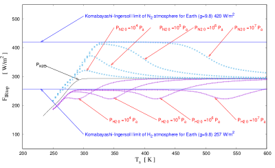
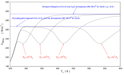
It is investigated the gray calculations for cases of background gases with H2 for m/s2. The relationships between and for several initial cases are presented in Fig. 1.
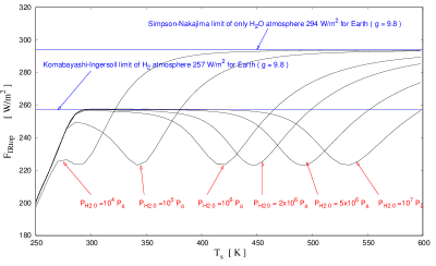
For H2 background atmosphere, it is characteristic that increases with surface temperature at the first time, however, it seems to reach the upper limit, then decrease down and again increase to reach the second saturated limit denoted as the SN-limit (Goldblatt & Watson 2012).
The first upper limit is due to the dominant H2 background atmosphere, where the optical depth is unity at the gas temperature K as shown in Figs. 2 and 3 where the case of Pa is presented. The decrease of after the first upper limit is due to the temperature decrease of the gas temperature corresponding to the region where the optical depth is about unity (later we call it as unity optical depth). After the lower limit of , it increases due to the temperature increase of the gas temperature corresponding to the unity optical depth which is shown in Fig. 2 and magnified in Fig. 3, where the detailed feature could be seen. The then increases to the SN-limit as shown in Fig. 1.
III.1 Moist tropospheric asymptotic limit (SN-limit)
There is a limit of that the initial of the background atmosphere is small or null where the atmosphere is consisted almost only of saturated H2O vapour. This is called the ”Moist tropospheric asymptotic limit”, ”Saturated vapour limit”, ”SN-limit” (Goldblatt & Watson 2012), or ”steam limit” (Koll & Cronin 2019). The second upper limit is the same with the only water vapour atmosphere, being the case of saturated vapour pressure ( 294 W/m2 for m/s2 and 340 W/m2 for super-Earth in Fig. 10).
When the surface temperature is enough high, the mole fraction of water vapour is almost unity and optical depth increases. When the optical depth is smaller than unity, the outgoing flux comes from the bottom of the Hydrogen atmosphere. However, when optical depth is greater than unity, the outgoing flux comes from the place where the optical depth is almost unity from the top of the atmosphere ( UOD: unity optical depth). Then the outgoing flux is almost the same as that of a pure H2O atmosphere.
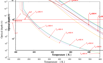
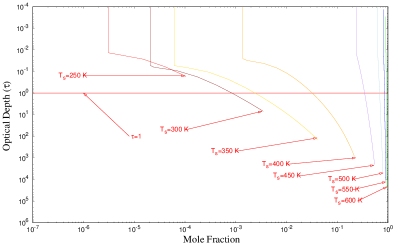
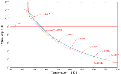
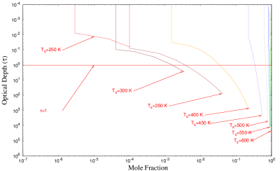
The relationships between surface temperature and optical depth of Pa for several cases are presented in Fig. 2. The cases of K, 300K, 350K, 400K, 450K, 500K, 550K, and 600K are presented by red, dark-red, brown, orange, purple, light-blue, blue, and green colour curve, respectively, The unit optical depth () is also presented by the red line and the magnified figure is presented in Fig. 3.
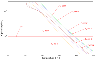
The luminosity is mainly radiated at around and the intensity is related to the local temperature of . The first bump of in Fig. 1 is appeared at K and then the luminosity decreases around K and then increases around K. The detailed features could be seen in Fig. 3 as the line of is crossed by each curve.
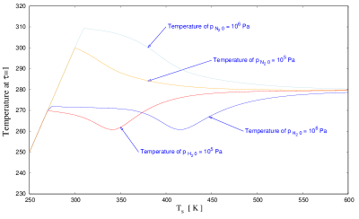
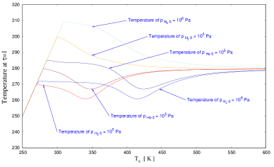
The features could be understood in Fig. 4, where the relationship between the temperature at UOD (Unity optical depth) and of Pa is presented by blue curves. The luminosity decreases around K and then increases around K. The case of Pa is shown there by red curve. The cases for N2 atmospheres of and Pa are also presented for reference by light blue and orange curves, respectively. For the case that the total optical depth is smaller than unity, the temperature of UOD is assumed to be equal to .
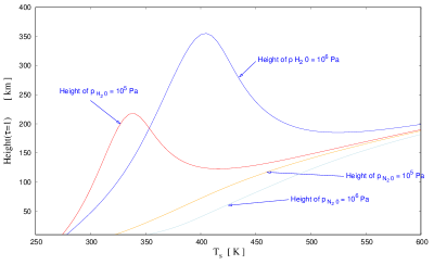
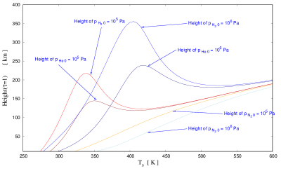
In Fig. 5, the relationships between the height of UOD and of is presented by blue and curve. The height of UOD has increased to km, where the temperature of UOD has decreased to 260 K (see Fig. 4). The case of Pa is shown there by red curve. The cases for N2 atmospheres of and Pa are also presented for reference by light blue and orange curves, respectively. The height of UOD is taken to be zero for the case that the total optical depth is smaller than unity.
In the low temperature limit, the lapse rate is assumed to be the dry adiabat, , as described in Pierrehumbert (2010) and Appendix B
| (10) |
where is the specific heat per unit mass and proportional to the inverse of the molecular weight . In Appendix B, it is investigated the analytical expression derived by Koll & Cronin (2019) for the OLR limit values of the steam limit and dilute limit. In Appendix C, it is tried to derive Eq. (33) in Koll & Cronin (2019) for suspected typos.
It should be noted that at 400 K for Pa the height of UOD has increased to km in H2, whereas km in N2. The main difference must be due to the low molecular weight of H2 relative to N2.
The increase of the UOD height is related to the features that increases with surface temperature at first time then decreases down and again increase to reach the second saturated limit. Thr first increase is due to the increase of and the lower value of the water vapoure (Figs. 6 and 7). The upper limit is due to the KI-limit. The decrease is due to the increase of the water vapour and the optical depth (Figs. 6, 7, and 8). The UOD height increase is related to the decrease the UOD temperature (Figs. 4 and 5). The second saturated limit is due to the increase and saturation limit of the water vapoure (Figs. 4 8).
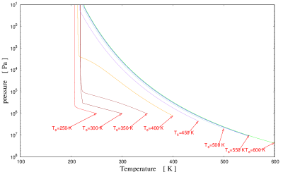
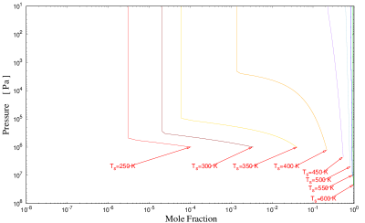
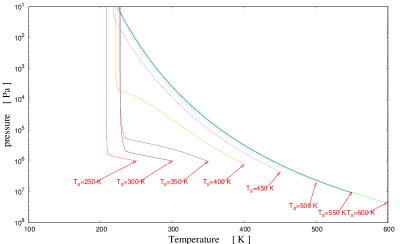
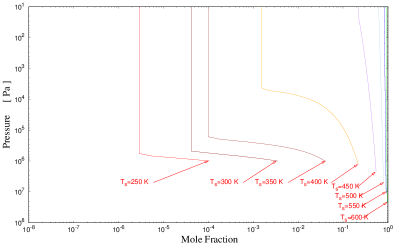
The relationships between temperature and pressure of Pa for several cases are calculated in Fig. 6 and the relationships between mole fraction and pressure are shown in Fig. 7. In Fig. 8, the relationships between mole fraction and optical depth are presented.
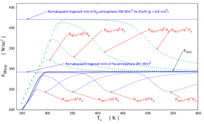
For H2 atmosphere, optical depth at tropopause is given by Eq. (9) where the factor increases about 10 from N2 to H2 atmosphere which causes the decrease of KI-limit ( 420 W/m2 (N2) to 257 W/m2 (H2), as shown in Fig. 9).
The difference between N2 and H2 background atmosphere is the difference of the mean molecular weight which corresponds to the change of the optical depth. For H2 atmosphere, the optical depth has increased. Even for the same surface temperature, the temperature at optical depth decreases for H2 atmosphere. Then the outgoing radiation has decreased for the H2 atmosphere compared to the N2 atmosphere.
If H2 pressure increases, the outline of the graph has moved to the right-hand which is shown in Fig. 1. If the surface temperature increased to the right-hand direction, there is a possibility that the ocean would evaporate.
The relationships between and for several and cases are presented in Fig. 9. Some H2 results in Fig. 1 are included in Fig. 9. The cases of N2 are almost the same given in Nakajima et al. 1992, except that the molecular weight of N2 is taken 28 (it is taken 18 in Nakajima et al. (1992) for its simplicity), then KI-limit has increased from 385 W/m2 to 420 W/m2.
The cases of H2 for super-Earth ( m/s2) are shown in Fig. 10.

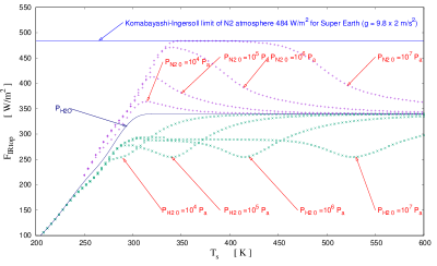
In Fig. 11, super-Earth cases of background gases with H2 and N2 are presented for the relationships between and in several initial cases. The arrow of shows the case of Pa which means only H2O atmosphere component corresponding to the SN-limit.
IV Applied to background atmosphere
The situations of He background atmosphere are similar to the case of H2 background atmosphere except the treatment of the mean molecular weight and the specific heat of He as R, being mono atomic gas, compared to that of H2, as R, being dipole atomic gas.
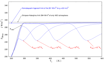
In Fig. 12, the results of He atmosphere are similar to those of H2 cases in Fig. 1. The first upper limit of and are the KI-limit of He atmosphere. Then they decrease down and increase approximately to the SN-limit as the cases of H2 background gas as presented in Fig. 1.
It must be noticed that the KI-limit for He atmosphere is 291 W/m2 which is almost the same value of the SN-limit 294 W/m2. It seems to be a problem that the SN-limit is greater than the KI-limit, however it is not a problem because the components of the background atmospheres have changed from He to H2O. It is almost the same for H2 atmosphere cases in Fig. 1.
It is pointed out by Koll & Cronin (2019) that H2 is the only background gas for which the dilute runaway (KI-limit) lies below the steam limit (SN-limit). However as shown in Fig 12, He is also the background gas for which the dilute limit lies below the steam limit.
The relationships between and optical depth of Pa for several cases are presented in Fig. 13. The =250K, 300K, 350K, 400K, 450K, 500K, 550K, and 600K are presented by red, dark-red, brown, orange, purple, light-blue, blue, and green colour curves, respectively, The unit optical depth () is also presented in red line.

Fig. 14 is the magnified figure of Fig. 13 to explain the change of for different of . The luminosity is mainly radiated at around and the intensity is related to the local temperature of . The first bump of Pa in Fig. 12 is appeared at K and then the luminosity decreases around K and then increases around K.
The features could be understood in Fig. 15, where the relationship between the temperature at UOD (Unity optical depth) and of Pa is presented by dark blue curves. The luminosity decreases around K and then increases around K. The case of Pa is shown there by dark red curve. The cases for H2 atmospheres of and Pa are also presented by blue and red curves, respectively. The cases for N2 atmospheres of and Pa are also presented for reference by light blue and orange curves, respectively. For the case that the total optical depth is smaller than unity, the temperature of UOD is assumed to be equal to .
In Fig. 16, the relationships between the height of UOD and of is presented by dark blue curve. The height of UOD has increased to km, where the temperature of UOD has decreased to 270 K (see Fig. 15). The case of Pa is shown there by dark red curve. The cases for H2 atmospheres of and Pa are also presented by blue and red curves, respectively. The cases for N2 atmospheres of and Pa are also presented for reference by light blue and orange curves, respectively. The height of UOD is taken to be zero for the case that the total optical depth is smaller than unity.
The relationships between temperature and pressure of Pa for several cases are presented in Fig. 17, and the relationships between mole fraction and pressure are shown in Fig. 18 The relationships between mole fraction and optical depth are calculated in Fig. 19.
To compare the cases of N2, the results of N2 and He are presented in Fig. 20 for =9.8m/s The relationships between and for several and cases are presented there. Several cases of in Fig. 12 are also included here. The case of pure H2O atmosphere is shown by black curve.
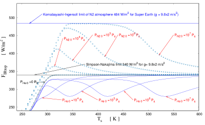
For super-Earth in m/s2, it is investigated the gray calculations for cases of background gases with He in Fig 21. The relationships between and for several cases are presented. The case of pure H2O atmosphere is shown by black curve. It is noticed that KI and SN-limits are different from Earth cases in Fig. 12.
It is investigated the gray calculations for cases of background gases with N2 and He for super-Earth case in Fig. 22. The relationships between and for several and cases are presented there. Several cases of in Fig. 21 are also included here.
V KI-limit dependence on the initial pressure
It is noticed that the KI-limit depends on the initial pressure of the background component as well as (molecular weight).
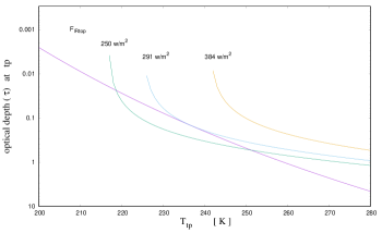
In Fig. 23, the relationship between the optical depth and the temperature is presented of He atmosphere for as a parameter with 250, 291, and 384 W/m2 in Pa. The coloured curves represent Eq. (8) for and the almost straight blue curve represents Eq. (9), where the suffix ”” means the value at the tropopause (Nakajima et al. 1992).
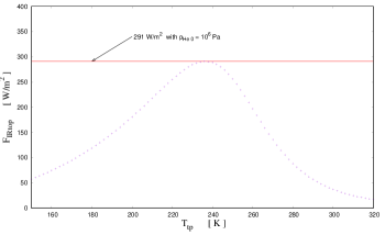
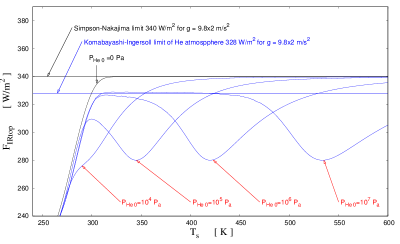
The relationship between and for Pa is shown in Fig. 24. The KI-limit of this model in He atmosphere is 291 W m-2 for Pa.
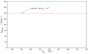
In Fig. 25, the relationship between and for Pa is presented where the KI-limit is 298 W/m2, which is different from 291 W/m2 for Pa. The KI-limit of He atmosphere is 291 298 W/m2 for Pa, which is shown in Fig. 26 as case for He. It shows that the KI-limit depends on the initial pressure of the background gas.
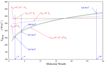
In Fig. 26, it is calculated the KI-limit dependence on molecular weight for fixed initial pressure of the background gases. The relationships between molecular weight and for each initial pressure of the background gases is presented. For example, in the case that the value of molecular weight is 18 where the molecular weight of every molecule is the same with water H2O, is the same for any initial pressure . On the other hand, in the He background atmosphere the mean molecular weight (MMW) for Pa, the KI-limit is W/m2 which is almost the same of , because the dominant component of the atmosphere is H2O. For Pa, KI-limit of is 291 W/m2 where the dominant component of the atmosphere is He. Even for fixed molecular weight of the background atmosphere, changes due to the increase of H2O compared to the initial component pressure. The KI-limit depends on the initial component pressure .
About the saturation vapour pressure on temperature, we take Eq. (2), so the results in Fig. 26 seem to be independent on any peculiar temperature.
VI Results and Discussion
We have presented the results of the outgoing radiation for the different components of background gas under a simple model with gray approximation adopted by Nakajima et al. 1992. The main results of the paper are the following:
1. It is studied the possibility of the various atmospheres over oceans.
2. H2 atmospheres as well as He are investigated. To our concern, the treating
He atmosphere in this style seems to be rather new.
3. The strange features are found for H2 atmosphere as well as He that increases
to the first upper limit, then decreases and increase again to the second limit :
named ”Souffl effect” by Koll & Cronin (2019).
4. The first upper limit is the Komabayashi-Ingersoll limit (KI-limit), which is not stated
explicitly by Koll & Cronin (2019).
5. The KI-limit value depends on the molecular weight and the initial pressure of
the background atmosphere (Sect. V).
6. The second limit is the Simpson-Nakajima limit (SN-limit) which is the atmosphere
mainly composed by vapour, called ’steam limit’ (Koll & Cronin 2019).
7. ”Souffl effect” is analysed by taking the UOD (Unit optical depth) temperature
which has decreased and the UOD height which has increased.
8. H2 atmosphere as well as He is the non-condensible background component where
the KI-limit is lower than the SN-limit.
9. The mixed gas of the relative realistic mixed atmosphere (H He
is investigated. The first upper limit is W/m2 (Sect. VI).
10. The various approximate limits derived by Koll & Cronin (2019) are investigated
and considered its applicability (Appendix B).
From the above consideration, it becomes clear that it must be considered the atmospheric components of the extra terrestrial planets if one want to investigate ”Habitable Zone”. We would like to expect much more observations further to find out the life trace in extra-terrestrial planets (Hill et al. 2022).
VI.0.1 Injection flux vs. Distance from a parent star
To apply the above results to the planet formation, it is better to consider the solar constant (1364 W/m2) for Earth orbit where the gravitational acceleration as 9.8m/s2. Taking the spherical mean for the injected flux ( 1/4), the flux becomes 341 W/m2.
As the solar luminosity is almost 70 of present value at 4.6 Gy ago (Bahcall, Pinsonneault, & Basu 2001), the flux is 239 W/m2. If we take the albedo 0.3 which is the corresponding value of Earth at present, the solar injection flux decreases to 167 W/m2.
The KI-limit for H2 atmosphere is 257 W/m2 which is greater than the above 239 W/m2 and 167 W/m2 values. Then it is stable for H2 atmosphere for assumed planets in Earth orbit. Even for super-Earth, the KI-limit for H2 atmosphere is 295 W/m2 which is greater than the above 239 W/m2and 167 W/m2 values. Then it is stable for H2 atmosphere for assumed super-Earth planets in Earth orbit.
The KI-limit for He atmosphere is 291 W/m2 which is greater than the above 239 W/m2 and 167 W/m2 values. Then it is stable for He atmosphere for the assumed planets in Earth orbit. Even for super-Earth, the KI-limit for He atmosphere is 328 W/m2 which is greater than the above 239 W/m2 and 167 W/m2 values. Then it is stable for He atmosphere for the assumed super-Earth planets in Earth orbit.
If the orbit has decreased to 0.5 Au, the injection flux increased four times as 956 (=239 4) W/m2 and 668 W/m2. Then it becomes unstable for Earth and super-Earth planets, because the situations are over the KI-limit and SN-limit. They will be in a greenhouse runaway and/or moist greenhouse situation.
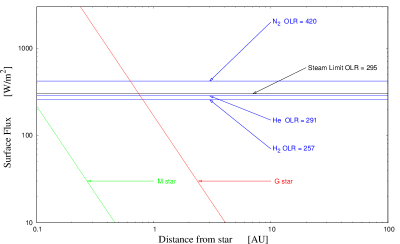
In Fig. 27, the injection flux versus the distance from parent star is shown. The star is taken for a G and an M host star by red and green line, respectively. For an M-type star the luminosity is taken with 1.3 % of the Sun (Pierrehumbert & Gaidos 2011). G star is normalized 167 W/m2 at 1AU. Three dilute limits for H2 ( 257 W/m2), He ( 291 W/m2), and N2 ( 420 W/m2) atmospheres and the steam limit ( 295 W/m2) are presented for reference. The steam limit is shown by black.
Under this model, it is found that the OLR upper limit decreases in the H2 rich atmosphere for the decrease of the mean molecular weight. Then it becomes clear that it is possible to become the runaway situation for super-Earth in the distance smaller than 1AU from the G type star (Sun). Even if OLR has not reached the upper limit, there is a possibility to become dry up the ocean due to the high surface temperature of the greenhouse effect.
If there are extra planets with H2 atmosphere over ocean and a life such as photosynthetic bacteria of the class Cyanobacteria (indicated by Pierrehumbert & Gaidos, 2011), it must be an unstable situation for the chemical reaction between H2 and O2. It could be a stable atmosphere with He and O2. We would like to estimate the diffusion time of H2 through the initial atmosphere mainly composed H2 and He (Sekiya, Nakazawa & Hayashi 1980; Wordworth 2012; Hu et al. 2015; Pahlevan et al. 2022).
VI.0.2 Mixed background gases with H2 and He
In Fig. 28, the gray calculations for mixed background gases with H2 (weight X) and He (weight Y for m/s2 are presented. This mixed gas is considered to be the primordial gas from which Sun and Earth are formed. The relationships between and for several initial and Pa) cases for Earth are shown. The first upper limit for this atmosphere is 267 W/m2), which has increased from H2 of 257 W/m2 (see Fig. 1). The second limit (steam limit) is the same of H2 and He as 294 W/m2.
VI.0.3 Various uncertainty
There are various uncertainty factors to estimate the relationship between the surface temperature and outgoing infrared radiation at the top of the atmosphere . Our results do not apply directly to any real planet history because of large uncertainties in our calculation due to the absence of clouds and the use of a one-dimensional model. In order to determine quantitatively, it seems to be necessary to evaluate the parameters such as albedo, effects of clouds, and relative humidity, circulation of the atmosphere over the surface of the planet (Manabe & Wetherald 1967, Zsom et al. 2013, Manabe & Broccoli 2020). It will be better to estimate the distribution of those parameters for the greenhouse effects and under the increase of solar luminosity.
a. gray opacity approximation
If one considers more than gray opacity approximation, one has to treat opacity, including the line by line treatments, Lorentz factor, pressure effect, random approximations, and further (Pierrehumbert 2010; Seager 2010), which make the physical understanding to be complicated.
Appendix A Derivation of the equation (3) in relation to Pierrehumbert (2010)
In this appendix, it is explained that the equation of (4) in Nakajima et al. (1992) (Eq. (3) in this paper) is equivalent to the equation of (2.33) in Pierrehumbert (2010). The notation is followed to Pierrehumbert (2010) and equation number is shown as (Pie. 2.33). As stated before, it is checked for the situation for the different molecular weights of condensible and non-condensible substances (Nakajima et al. have assumed the same for simplicity).
The equation in (Pie. 2.33) is written as
| (A.1) |
where subscript and are related to non-condensible and condensible substance, respectively. Other notations are the following.
A partial pressure of non-condensible substance is described as which is related to total pressure as where is the partial pressure of condensible substance (water vapour). Then . It is introduced saturation assumption that is replaced by . Using Clausius-Clapeyron to re-write that
| (A.2) |
where is the gas constant for the substance which is condensing (water) as shown in (Pie. 2.25) and is the latent heat associated with the transportation to the more condensed phase.
Then of the second term in (Pie. 2.32) becomes as
| (A.3) |
So the second term in (Pie. 2.32) is written as
The term of is moved to the first term of (Pie. 2.32).
Then the equation of (Pie. 2.32) becomes for taking as
| (A.4) |
| (A.5) |
Then taking and where and are molecular weight of the substanc a (=n: non-condensible background substance, eg. H2, He, N2, and air: suffix ’a’ comes from Pierrehumbert and ’n’ comes from Nakajima et al.), and c (=v: condensible substance, eg. water vapour), the above equations have changed to the followings.
Using , the square bracket of Eq. (A. 4) becomes as
where we use .
The square bracket of Eq. (A. 5) becomes as
Considering , the equation (Pie. 2.33) becomes as
| (A.6) |
where we neglect the differences between partial derivative and total derivative, and take and . When
Then the derivation of equation (4) in Nakajima et al. is equivalent to the equation of (Pie. 2. 33).
It is also equivalent to the equations of (3.7) and (3.14) in Houghton (1977)
| (A.7) |
and
| (A.8) |
If the term in the denominator is neglected for its small values, the above two equations becomes equivalent to the equation (3) in this paper and equation of (4) in Nakajima et al. (1992).
Appendix B Trial to derive the limit values
B.1 MMW matters (Koll & Cronin 2019)
First, taking the water vapour scale height , the optical depth is
| (B.1) |
where (in general, the subscript will denote quantities related to water vapour).
Using the ideal gas law for water vapour, where is the saturation vapour pressure, and the Clausius-Clapeyron relation, ln ln where is the latent heat of vapourization:
| (B.2) |
and
| (B.3) |
where is used.
Here it is denoted as the temperature scale height, which is related to the water vapour scale height as
| (B.4) |
then it is accepted for water vapour and a wide range of other condensible gases.
In the low temperature limit, the lapse rate is assumed to be the dry adiabat, , and
| (B.5) |
At high temperature the total pressure is dominated by the saturation vapour pressure of water and the temperature scale height is given by
| (B.6) |
where the hydrostatic equation, , is used.
It should be noted that at a temperature of 400 K with an Earth-like gravity, km in H2, whereas km in N2. The main difference is due to the low molecular weight of H2 relative to N2 (see Fig. 5).
B.2 Trial to derive the steam and dilute limit values
Koll & Cronin (2019) have tried to derive an approximate analytical expression for the OLR limit values of the steam limit (SN-limit) and dilute limit (KI-limit). They have approximated the saturation pressure with temperature as
| (B.7) |
taking the Clausius-Clapeyron relation d ln d ln . They have expressed the relation between optical depth and temperature as a power law (see Koll & Cronin 2019)
| (B.8) |
where is a reference temperature close to the interest range.
OLR is said to be equal to
| (B.9) |
the first term can be neglected as optical depth increasing and the upper limit of the integral is replaced with infinity
| (B.10) | |||
| (B.11) | |||
| (B.12) | |||
| (B.13) |
Here is the gamma function, defined by exp, and denotes for steam limit
| (B.14) |
and for dilute limit
| (B.15) |
where it is taken for H2 and N2 diatomic molecule and for He monoatomic molecule. The latent heat is tentatively taken, for the moment, as (J/g), where 2265 (J/) is the vapourization energy per gram at 373K and 4.186 (J/( K)) is the specific heat of water, approximately.
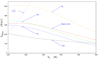
Dilute limit dependence on for H2, He, and N2 atmospheres given by Eqs. (B.13) and (B.15) are presented by blue, green, and orange curve in Fig. 29, respectively. For the steam limit given by Eqs. (B.13) and (B,14) is presented by red curve in Fig. 29. They are almost constant or monotonically decreasing with , however the value of has changed which is shown for reference by purple curve in Fig. 29.
Taking and , for is taken as a mean value of as where
| (B.16) |
being i (=1, 2) and . Ten times of is presented in Fig. 29 in black curve as and some values are shown in Table I.
It must be noticed that He dilute limit (green line) lies below the steam limit (red line) beyond K, which is not indicated by Koll & Cronin 2019.
For taking K where , OLR W/m2 for steam limit (calculated result is W/m2 (Fig. 1); then 316/2941.075: the difference is 7.5%). The dilute limit of H2 atmosphere is W/m2 (calculated result is W/m2 (Fig. 1), then 280/257 1.089: the difference is 8.9 %). The dilute limit of He atmosphere is W/m2 (calculated result is 291 W/m2 (Fig. 12), then 328/291 1.127: the difference is 13 %). The dilute limit of N2 atmosphere is W/m2 (calculated result is W/m2 (Fig. 9), then 511/420 1.217: the difference is 22 %).
Although they have shown some limiting values, it seems to be a little bit difficult to accept that the limiting values could approximately represent the calculated values. The absolute limiting values seems to have some differences (dilute limit of N2 differs about 22 %) for 300K and (dilute limit of H2 is only about 32 % (differs 68 %) for 500K. They are shown in Fig. 29 and particular values are presented in Table I.
Let us consider the limiting values from the different point. The relative differences of the limiting values could be understood by the above Eq. (B.14).
1. The difference of the accelerating gravity: if has changed to by factor , has changed to and OLR∞ has changed by factor . Taking and , it becomes . The steam limit has changed from 294 W/m2 (Fig. 1) to 340 W/m2 (Fig. 10) which is almost the same as ). The difference is within 1.3%. . The dilute limit for H2, it has changed from 257 W/m2 (Fig. 1) to 295 W/m2 (Fig. 10) where 295/257 1.1479 (1.1711/1.1479 1.0202). The difference is within 2.1 %. The dilute limit for He, it has changed from 291 W/m2 (Fig. 12) to 328 W/m2 (Fig. 21) where 328/291 1.12714 (1.1711/1.2714 0.9211). The difference is within 7.9 %. The dilute limit for N2, it has changed from 420 W/m2 (Fig. 9) to 484 W/m2 (Fig. 22) where 480/420 1.14286 (1.1711/1.14286 1.0247). The difference is within 2.5 %.
2. The difference of the mean molecular weight: is the specific heat per gram related to the specific heat per mol where is the molecular weight. Then if the molecular weight has increased by factor , has decreased by factor . The has changed to and OLR∞ has changed by factor . Taking from H2 to He and , it becomes . The dilute limit has changed from 257 W/m2 (Fig. 1) to 291 W/m2 (Fig. 12) which is almost the same as 291/257 ). The difference is within 3.5 %.
Taking from H2 to N2 and , it becomes . The dilute limit has changed from 257 W/m2 (Fig. 1) to 420 W/m2 (Fig. 9) which is almost the same as 420/257 ) . The difference is within 12 %.
Taking from He to N2 and , it becomes . The dilute limit has changed from 291 W/m2 (Fig. 12) to 420 W/m2 ( Fig. 9)which is almost the same as 420/291 The difference is within 8.0 %.
It is a rather good approximation to estimate the OLR∞ by the variation of gravity (differences are within 7.9 %) and molecular weight (differences are within 12 %).
| K | SL | R1 | H | R2 | He | R3 | N | R4 | |
|---|---|---|---|---|---|---|---|---|---|
| 300 | 17.55 | 316 | 1.078 | 280 | 1.089 | 328 | 1.126 | 511 | 1.216 |
| 350 | 15.03 | 286 | 0.975 | 233 | 0.905 | 280 | 0.961 | 469 | 1.117 |
| 400 | 13.15 | 238 | 0.813 | 176 | 0.684 | 217 | 0.746 | 393 | 0.935 |
| 450 | 11.68 | 187 | 0.639 | 123 | 0.480 | 156 | 0.537 | 304 | 0.725 |
| 500 | 10.51 | 140 | 0.479 | 81.2 | 0.316 | 106 | 0.363 | 222 | 0.528 |
In the Table I the particular values of , the steam limit and the dilute limit for of H2, He and N2 are shown, where SL, H2, He and N2 represent steam limit, dilute limit of H2, He and N2, respectively. R1, R2, R3 and R4 show the ratio of the approximate value to the calculated value, as SL/293, H2/257, He/ 291 and N2/420, respectively. For example in K, the difference of the steam limit is 7.8 %. The difference of the dilute limit of H2 is 8.9 %. If has changed to 500 K, the differences have increased much further.
From the values in the Table I, the approximate analytical expressions seems to be applicable in the temperature K where the differences are within and around 20 % (not bad). For K, the differences are worse than 20 %. The reason is not so clear for the moment.
Appendix C Try to derive Eq. (33) in Koll & Cronin (2019)
We have tried to derive the following three equations in Koll & Cronin (2019),
where (KC 32) represents Eq. (32) in Koll & Cronin (2019) and so on.
Using = and , the equation of (KC 32) becomes
where we use the relation , and . It must be noticed that signatures in and out of the parentheses are different from (KC 33). We believe that those are typos.
Using the Clausius-Clapeyron relation, , Eq. (KC 34) becomes as
where it must be noticed that the signature of the term in the parenthsis is exact of Eq. (KC 34).
References
- (1)
- (2) [] When the altitude rises above the sea level and the pressure drops, the liquid precipitates, but since the liquid does little work, the approximation here is to omit the contribution of the liquid from the system. Therefore, since the reversibility is lost from the equation dS = 0, it is described as quasiadiabat.
- (3) [Betts, H. C., Puttick, M. N., Clark, J. W., et al.] 2018, Nature Ecology & Evolution, 2, 1556,
- (4) [Bressler, S., & Shaviv, G.,] 2015, Astronomical Rev. 11, 41.
- (5) [Goldblatt C., Robinson T.D., Zahnle K. J., & Crisp D.] 2013, Nature Geosci. 6, 661.
- (6) [Goldblatt C., & Watson A. J.] 2012, Phil. Trans. R. Soc. A370, 4197.
- (7) [Hara T., & Suzuki A.] 2021, SCIREA J. Physics, 6, 154, (https://doi.org/10.54647/physics14381; arXiv: 2009.04040),
- (8) [Hill L. M., Bott K., Dalba A. P., Fetherolf T., Kane R. S., Kopparapu R., Li Z., & Osberg C.] 2022, arXiv:2210.02484v1.
- (9) [Houghton J. T.] 1977, The Physics of Atmospheres, Cambridge Univ. Press, Cambridge, UK.
- (10) [Hu R., Seager S., & Yung Y. L.] 2015, ApJ, 807, 8.
- (11) [Ingersoll A. P.] 1969, J. Atmos. Sci. 26, 1191.
- (12) [Kasting J.F.] 1988, Icarus, 74, 472.
- (13) [Koll D.D.B., & Cronin T. W.] 2019, ApJ. 881,120.
- (14) [Komabayashi M.] 1967, J. Meteor. Soc. Japan, 45, 137.
- (15) [Madhusudhan N., Piette A.A.A., & Constantinou S.] 2021, arXiv:2108.10888v2.
- (16) [Manabe S., & Broccoli A. J.] 2020, Beyond Global Warming: How Numerical Models Revealed the Secrets of Climate Change, Princeton Univ. Press, Princeton, NJ.
- (17) [Manabe S., & Wetherald R.T.] 1967, J. Atmos. Sci., 24, 241.
- (18) [Nakajima S., Hayashi Y., & Abe Y.] 1992, J. Atmospheric. Scie. 23, 2256.
- (19) [Pahlevan K, Schaefer L., Elkins-Tanton L., Desch J. S, & Buseck R. P.] 2022. arXiv: 2209.10635.
- (20) [Pierrehumbert R.T.] 2010, Exoplanet Atmosphere: Physical Process, Cambridge Univ. Press, Cambridge, UK.
- (21) [Pierrehumbert R., Gaidos, E.] 2011, ApJ, 734, L13.
- (22) [Seager S.] 2010, Exoplanet Atmosphere: Physical Process, Princeton Univ. Press, Princeton, NJ.
- (23) [Sekiya M., Nakazawa K., & Hayashi C.] 1980, EPSL, 50, 197.
- (24) [Sekiya M., Nakazawa K., & Hayashi C.] 1981, Prog. Theor. Phys. 66, 1301.
- (25) [Simpson, G. C. ] 1927, Mem. R. Meteorol. Soc. 11, 69.
- (26) [Suzuki A.] Part of the work was postered at Quy Nhon, Vietnam (Dec. 11-17, 2016). 2017, Master thesis at Kyoto Sangyo University in Japanese.
- (27) [Wordsworth R.,] 2012, Icar, 219, 267.
- (28) [Wordsworth R., Pierrehumbert R., & Del Genio A.D.] 2013, Science 339, Issue 6115, 64.
- (29) [Zsom A., Seager S., de Witt J., & Stamenkovic V.] 2013, ApJ, 778, 109.