Abstract

We systematically study the chaotic signatures in a quantum many-body system consisting of an ensemble of interacting two-level atoms coupled to a single-mode bosonic field, the so-called extended Dicke model. The presence of the atom-atom interaction also leads us to explore how the atomic interaction affects the chaotic characters of the model. By analyzing the energy spectral statistics and the structure of eigenstates, we reveal the quantum signatures of chaos in the model and discuss the effect of the atomic interaction. We also investigate the dependence of the boundary of chaos extracted from both eigenvalue-based and eigenstate-based indicators on the atomic interaction. We show that the impact of the atomic interaction on the spectral statistics is stronger than on the structure of eigenstates. Qualitatively, the integrablity-to-chaos transition found in the Dicke model is amplified when the interatomic interaction in the extended Dicke model is switched on.

1 1 0 https://doi.org/ Quantum Chaos in the Extended Dicke Model Qian Wang ^2,1 Qian Wang Wang, Q.

1 Introduction

In recent years, the study of quantum chaos in many-body systems has attracted much attention, both theoretically and experimentally, in different fields of physics, such as statistical physics Altland and Haake (2012); D’Alessio et al. (2016); Borgonovi et al. (2016); Nandkishore and Huse (2015); Deutsch (2018), condensed matter physics Chan et al. (2018); Garcia-March et al. (2018); Friedman et al. (2019); Ray et al. (2020); Rautenberg and Gärttner (2020); Kobrin et al. (2021); Fogarty et al. (2021); Wittmann W. et al. (2022), high energy physics Maldacena et al. (2016); Stanford (2016); Magán (2018); Jahnke (2019); Ali et al. (2020); Rabinovici et al. (2021), as well as quantum information science Schack and Caves (1996); Vidmar and Rigol (2017); Piga et al. (2019); Bertini et al. (2019); Lerose and Pappalardi (2020); Lantagne-Hurtubise et al. (2020); Anand et al. (2021). To some extent, this great interest in quantum many-body chaos is due to the close connections of chaos to several fundamental questions that arise in current theoretical and experimental studies. Although a full understanding of quantum many-body chaos is still lacking, much progress has been achieved. It is known that chaos in interacting quantum many-body systems can lead to thermalization Altland and Haake (2012); D’Alessio et al. (2016); Borgonovi et al. (2016), the fast scrambling of quantum information Maldacena et al. (2016); Hosur et al. (2016); Chenu et al. (2019); Prakash and Lakshminarayan (2020), an exponential growth of quantum complexities Ali et al. (2020); Balasubramanian et al. (2020); Bhattacharyya et al. (2021a, b); Parker et al. (2019); Dymarsky and Gorsky (2020); Caputa et al. (2022), and diffusive transport Bertini et al. (2021).

The notion of chaos in the classical regime is usually defined by the so-called butterfly effect, namely the exponential separation of inifitesimally nearby trajectories for initial perturbations Cvitanovic et al. (2005); Schuster and Just (2006). However, as the concept of trajectory is ill-defined in quantum mechanics, the definition of quantum chaos remains an open question. Therefore, to probe the signatures of chaos in quantum many-body systems becomes a central task in the studies of quantum many-body chaos. To date, many complementary detectors of quantum chaos and the limits of their usefulness have been widely investigated in literature Chenu et al. (2019); Bohigas et al. (1984); Stöckmann (1999); Haake (2010); Zyczkowski (1990); Emerson et al. (2002); Bhattacharyya et al. (2021a, b); Parker et al. (2019); Rozenbaum et al. (2017); García-Mata et al. (2018); Chen and Ludwig (2018); Kos et al. (2018); Bertini et al. (2018); Gietka et al. (2019); Xu et al. (2020); Cao et al. (2021); Zonnios et al. (2022); Raúl González Alonso et al. (2022); Joshi et al. (2022). Important model systems in this context are billiards Stöckmann (1999); Lozej et al. (2022). Another task, which has recently also drawn great interest, is to unveil different factors that affect the chaotic properties of quantum many-body systems. While the impacts of the strength of disorder and the choice of initial states on the development of quantum chaos in various many-body systems have been extensively explored Nandkishore and Huse (2015); Abanin et al. (2019); Turner et al. (2018); Sinha and Sinha (2020); Turner et al. (2021); Mondragon-Shem et al. (2021); Serbyn et al. (2021), more works are required in order to get deeper insights into the universal aspects of quantum many-body chaos.

In the present work, we analyze the emergence of chaos in the extended Dicke model. There are several different versions of the extended Dicke model Kloc et al. (2017); Rodriguez et al. (2018); Guerra et al. (2020); Herrera Romero et al. (2022). Here, we focus on the one that has been discussed in Ref. Rodriguez et al. (2018). Different from the original Dicke model Dicke (1954), which consists of an ensemble of noninteracting two-level atoms interacts with a single bosonic mode, the atoms in our considered extended Dicke model are permitted to interact. This allows us to analyze the effects of the atomic interaction on the degree of chaos of the model. Previously, the role of the atom-field coupling in the Dicke model for the emergence of quantum chaos has been investigated Emary and Brandes (2003); Wang and Robnik (2020); Bastarrachea-Magnani et al. (2015, 2016), while here we explore how this transition is affected by additional atomic interaction. By performing a detailed analysis of the energy spectral statistics and the structure of eigenstates, we systematically study both the chaotic signatures of the extended Dicke model and examine the effect of the atomic interaction on the chaotic features in the model. We show how the atomic interaction affects the spectral statistics and the structure of eigenstates, respectively.

The article is structured as follows. The model is introduced in Sec. 2. The influences of the atomic interaction on the energy spectral statistics are discussed in Sec. 3. The detailed investigation of the consequence of the atomic interaction on the structure of eigenstates is presented in Sec. 4. Finally, we conclude in Sec. 5 with a brief summarize of our results and outlook.

2 Extended Dicke model

As an extension of the original Dicke model Dicke (1954); Emary and Brandes (2003); Wang and Robnik (2020), the extended Dicke model studied here consists of $N$ mutual interacting two-level atoms with energy gap $\omega_{0}$ coupled to a single cavity mode with frequency $\omega$. By employing the collective spin operators $J_{x,y,z}=\sum_{i=1}^{N}\hat{\sigma}_{x,y,z}^{(i)}$ ($\hat{\sigma}_{x,y,z}$ are the Pauli matrices), the Hamiltonian of the extended Dicke model can be written as (hereafter we set $\hbar=1$) Robles Robles et al. (2015); Rodriguez et al. (2018)

$$H=\omega a^{\dagger}a+\omega_{0}J_{z}+\frac{2\lambda}{\sqrt{N}}J_{x}(a+a^{\dagger})+\frac{\kappa}{N}J_{z}^{2},$$ (1)

where $a(a^{\dagger})$ denotes the bosonic annihilation (creation) operator, $\lambda$ is the coupling stength between atom and field, and $\kappa$ represent the strength of the atomic interaction.

The conservation of total spin operator $\mathbf{J}^{2}=J_{x}^{2}+J_{y}^{2}+J_{z}^{2}$ for the Hamiltonian (1) leads to the Hamiltonian matrix being block diagonal in $\mathbf{J}^{2}$ representation. In this work, we will focus on the maximum spin sector $j=N/2$, which involves the experimental realizations and includes the ground state. Moreover, the commutation between Hamiltonian (1) and the parity operator $\Pi=e^{i\pi(j+J_{z}+a^{\dagger}a)}$ enables us to further separate the Hamiltonian matrix into even- and odd-parity subspaces. Here, we will restrict our study to the even-parity subspace.

To numerically diagonalize the Hamiltonian (1), we work in the usual Fock-Dicke basis $\{|n,m\rangle\}=\{|n\rangle\otimes|j,m\rangle\}$. Here, $|n\rangle$ are the Fock states of bosonic mode with $n=0,1,2,\ldots,\infty$ and $|j,m\rangle$ represent the so-called Dicke states with $m=-j,-j+1,\ldots,j$. Then, the elements of the Hamiltonian matrix are given by

$$\langle n^{\prime},m^{\prime}|H|n,m\rangle= (n\omega+m\omega_{0})\delta_{n^{\prime},n}\delta_{m^{\prime},m}+\frac{\kappa}{N}m^{2}\delta_{m^{\prime},m}+\frac{\lambda}{\sqrt{N}}\left[\sqrt{n}\delta_{n^{\prime},n-1}+\sqrt{n+1}\delta_{n^{\prime},n+1}\right]$$

$$\times\left[\sqrt{j(j+1)-m(m+1)}\delta_{m^{\prime},m+1}+\sqrt{j(j+1)-m(m-1)}\delta_{m^{\prime},m-1}\right].$$ (2)

We remark that the value of $n$ is unbounded from above, the actual dimension of the Hilbert space is infinite, regardless of the value of $j$. In practice, we need to cut off the bosonic number states at a larger but finite value $\mathcal{N}_{c}$. Moreover, the dependence of the chaoticity in the Dicke model on the energy Rodriguez et al. (2018); Cejnar et al. (2011); Chávez-Carlos et al. (2019) further implies that it is also necessary to cut off the energy in order to get the finite number of considered states. In our numerical simulations, we set $\mathcal{N}_{c}=320$ and restrict our analysis on the eigenstates with energies $E/N\in[0.4,4]$, the convergence of our results has been carefully examined. For our selected energy interval, we have checked that our main results are still hold for other choices of $\mathcal{N}_{c}$, as long as $N\geq 16$ and the convergence of Fock-Dicke basis is fulfilled.

The extended Dicke model exhibits both ground state and excited state quantum phase transitions and displays a transition from integrable to chaotic behavior with increasing the system energy, like in the Dicke model. The features of these transitions have been extensively investigated in the semiclassical regime Rodriguez et al. (2018). It is worth to mention that several possible experimental realizations of the extended Dicke model have been pointed out in Refs. Rodríguez-Lara and Lee (2011); Robles Robles et al. (2015); Rodriguez et al. (2018)

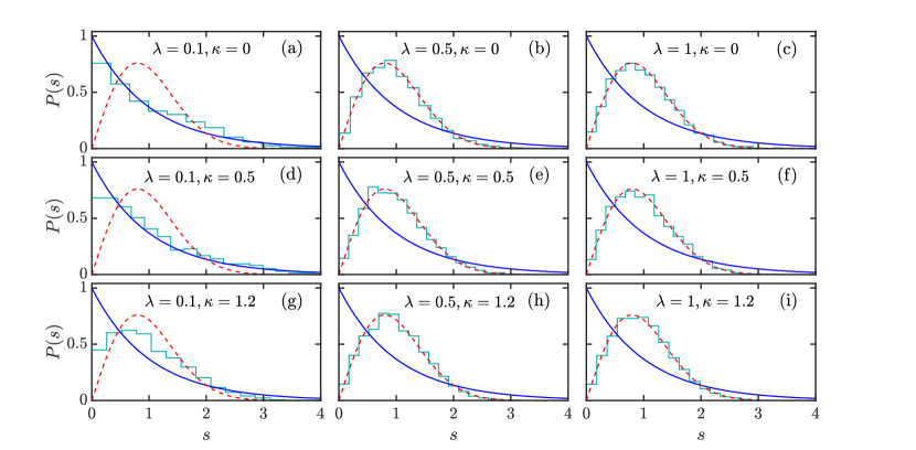
Figure 1: Level spacing distribution of the extended Dicke model for several combinations of $\lambda$ and $\kappa$. The considered energy levels are the ones that have energies $E/N\in[0.4,4]$. The total atom number is $N=2j=32$ and the cut off in bosinic Hilbert space is $\mathcal{N}_{c}=320$. The Poissonian (blue solid lines) and Wigner-Dyson distributions (red dashed lines) are, respectively, plotted in each panel for comparison. Other parameters are: $\omega=\omega_{0}=1$. All quantities are dimensionless.

3 Energy spectrum statistics

In this section we will explore the transition from integrable regime to chaos in the extended Dicke model by analyzing its energy level spacing distribution. In our study, we focus on the energy levels with energies change from $E/N=0.4$ to $E/N=4$. We will compare our results to the level distributions of fully integrable and chaotic cases, respectively. We are aiming to characterize the quantum signatures of chaos in the model and unveil the impact of the atomic interaction on its chaotic properties.

3.1 Level spacing statistics

As the most frequently used probe of quantum chaos, the distribution $P(s)$ of the spacings $s$ of the consecutive unfolded energy levels quantifies the degree of correlations between levels. For integrable systems, where the energy levels are allowed to cross, the distribution $P(s)$ is given by the Poissonian distribution Berry and Tabor (1977),

$$P_{P}(s)=\exp(-s).$$ (3)

On the other hand, the energy levels in chaotic systems exhibit level replusion and the distribution $P(s)$ follows the Wigner-Dyson distribution Bohigas et al. (1984); Stöckmann (1999); Haake (2010). For the systems with symmetric and real Hamiltonian matrices, as in the extended Dicke model, the Wigner-Dyson distribution has the following expression

$$P_{WD}(s)=\frac{\pi s}{2}\exp\left(-\frac{\pi}{4}s^{2}\right).$$ (4)

In Fig. 1, we show $P(s)$ of the extended Dicke model with $\omega=\omega_{0}=1$ and $j=N/2=16$ for different values of $\lambda$ and $\kappa$. Here, the level spacings $s$ are obtained from the unfolded eigenlevels $\tilde{E}_{\mu}=E_{\mu}/\Delta E$ with $1/\Delta E$ being the local density of states. One can clearly see that $P(s)$ undergoes a transition to Wigner-Dyson distribution as $\lambda$ increases, regardless of the value of $\kappa$. The case $\kappa=0$ is the original Dicke model as in our previous work Wang and Robnik (2020). However, we find that, with increasing $\kappa$, the Poissonian distribution at $\lambda=0.1,\kappa=0$ in Fig. 1(a) turns into an intermediate case, as observed in Fig. 1(g). This suggests that the degree of chaos in the extended Dicke model can be tuned by the atomic interaction.

To quantitatively characterize the effect of the atomic interaction on the degree of chaos, we consider the proximity of $P(s)$ to Wigner-Dyson or to Poissonian distributions. There are several ways to measure the distance between two distributions, here, the difference between $P(s)$ and $P_{WD}(s)[P_{P}(s)]$ is quantified by the chaos indicators $\eta$ and $\beta$. The indicator $\eta$ is defined as Jacquod and Shepelyansky (1997); Emary and Brandes (2003); Garcia-March et al. (2018)

$$\eta=\left|\frac{\int_{0}^{s_{0}}\left[P(s)-P_{WD}(s)\right]ds}{\int_{0}^{s_{0}}\left[P_{P}(s)-P_{WD}(s)\right]ds}\right|,$$ (5)

where $s_{0}=0.4729\ldots$ is the first intersection point of $P_{WD}(s)$ and $P_{P}(s)$. For $P(s)=P_{WD}$, we have $\eta=0$, while $P(s)=P_{P}(s)$ leads to $\eta=1$. The indicator $\beta$ is the level repulsion exponent and can be obtained by fitting $P(s)$ to the Brody distribution Brody et al. (1981)

$$P_{B}(s)=b_{\beta}(\beta+1)s^{\beta}\exp[-b_{\beta}s^{\beta+1}],$$ (6)

where the factor $b_{\beta}$ is given by

$$b_{\beta}=\left[\Gamma\left(\frac{\beta+2}{\beta+1}\right)\right]^{\beta+1},$$ (7)

with $\Gamma(x)$ being the gamma function. The value of $\beta$ varies in the interval $\beta\in[0,1]$. When $\beta=0$, it means the level spacing distribution $P(s)$ is Poisson. On the other hand, for chaotic systems, we would expect $P(s)=P_{WD}(s)$ and therefore $\beta=1$.

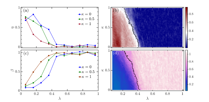
Figure 2: (a) Chaos indicator $\eta$ as a function of $\lambda$ for several values of $\kappa$. (b) $\eta$ as a function of $\kappa$ and $\lambda$. (c) Chaos indicator $\beta$ as a function of $\lambda$ for different values of $\kappa$. (d) $\beta$ as a function of $\kappa$ and $\lambda$. These results are obtained from the energy levels with energies $E/N\in[0.4,4]$. In panels (b) and (d), the boundary of the chaotic region are marked by the black curves, which are defined as $\eta\leq 0.3$ and $\beta\geq 0.7$, respectively. Other parameters are: $\omega=\omega_{0}=1$ and $N=2j=32$. All quantities are dimensionless.

In Fig. 2(a), we plot $\eta$ as a function of $\lambda$ for various values $\kappa$. It can be seen that irrespective of the strength of the atomic interaction, the extended Dicke model undergoes a transition from integrability to chaos as the coupling strength $\lambda$ increases. However, as the strength of the atomic interaction increases, the onset of chaos happens for smaller values of coupling strength $\lambda$. This is more evident from Fig. 2(b), where we show how $\eta$ evolves as a function $\kappa$ and $\lambda$. Clearly, the width of the region with larger values of $\eta$ decreases with increasing $\kappa$, suggesting that the location of the crossover to quantum chaos moves towards the lower values of $\lambda$ with increasing $\kappa$. The statement above is further confirmed by the boundary of chaotic region, which plots as the black curve in Fig. 2(b). Here, we determine the boundary of chaos by the condition $\eta\leq\eta_{d}=0.3$ Jacquod and Shepelyansky (1997). We set the threshold $\eta_{d}=0.3$ as it implies that the model has already departed from the integrablity and is tending to the chaotic regime.

Fig. 2(c) shows $\beta$ as a function of $\lambda$ with increasing $\kappa$. As observed in Fig. 2(a), while the chaotic behavior at higher values $\lambda$ is independent of $\kappa$, the coupling strength $\lambda$ that needs to be for the transition to chaos decreases with increasing $\kappa$. Fig. 2(d) illustrates $\beta$ as a function of $\kappa$ and $\lambda$. One can see that with increasing $\kappa$ the region with $\beta\approx 1$ extends to smaller values of $\lambda$. By identifying the chaotic region as $\beta\geq 0.7$, we show that the boundary of chaos strongly depends on the strength of the atomic interaction, see the black curve in Fig. 2(d). Notice that the boundary extracted from $\eta$ behaves in a similar way to the one exteracted from $\beta$.

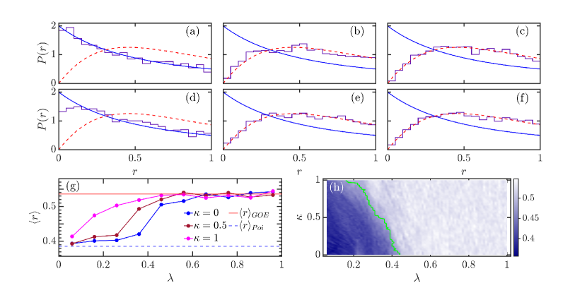
Figure 3: Level spacing ratio distributions $P(r)$ for various combinations of $\kappa$ and $\lambda$: (a) $\kappa=0,\lambda=0$, (b) $\kappa=0,\lambda=0.5$, (c) $\kappa=0,\lambda=1$, (d) $\kappa=0.7,\lambda=0$, (e) $\kappa=0.7,\lambda=0.5$ and (f) $\kappa=0.7,\lambda=1$. In each panel, the Poisson distribution $P_{Poi}(r)$ is plotted as blue solid curve, while the red dashed line denotes $P_{GOE}(r)$. (g) Averaged level spacing ratio $\langle r\rangle$ as a function of $\lambda$ for several values of $\kappa$. (h) $\langle r\rangle$ as a function of $\kappa$ and $\lambda$. The green line indicates the chaotic boundary, which is determined by $\langle r\rangle\geq 0.48$. The energy levels used in our numerical calculation have energies $E/N\in[0.4,4]$. Other parameters: $\omega=\omega_{0}=1$ and $N=2j=40$. All quantities are dimensionless.

3.2 Level spacing ratio

The study of level spacing distribution requires the so-called unfolding precedure Guhr et al. (1998). It proceeds by rescaling the original eigenlevels to ensure that the local density of states of the resulting spectrum is $1$. It is usually a non-trivial task, in particular, for quantum many-body systems. To circumvent this disadvantage, one can resort to another chaotic probe based on the ratio of adjacent level spacings Oganesyan and Huse (2007), which is free from unfolding procedure.

For a given set of level spacing $\{s_{\mu}=E_{\mu+1}-E_{\mu}\}$, the ratio of adjacent level spacings is defined as Oganesyan and Huse (2007); Atas et al. (2013a)

$$r_{\mu}=\mathrm{min}\left(\delta_{\mu},\frac{1}{\delta_{\mu}}\right),$$ (8)

where $\delta_{\mu}=s_{\mu+1}/s_{\mu}$ is the ratio between two adjacent level spacing. Obviously, $r_{\mu}$ is defined in the interval $r_{\mu}\in[0,1]$. The distribution of $r_{\mu}$ for both integrable and chaotic systems has been analytically investigated Atas et al. (2013a, b); Giraud et al. (2022). It has been known that for the chaotic systems with Hamitonian from the Gaussian orthogonal ensemble (GOE), the level spacing ratio distribution is given by

$$P_{GOE}(r)=\frac{1}{Z_{1}}\frac{2(r+r^{2})}{(1+r+r^{2})^{5/2}},$$ (9)

where $Z_{1}=8/27$ is the normalization constant. On the other hand, as the eigenlevels in the integrable systems are uncorrelated (independent Poisson levels), one can simply find the ratio distribution is

$$P_{Poi}(r)=\frac{2}{(r+1)^{2}}.$$ (10)

Due to $r_{\mu}\in[0,1]$, the ratio distribution $P_{GOE/Poi}(r)$ vanishes outside the range $[0,1]$.

Figs. 3(a)-3(f) show how the level spacing ratio distribution $P(r)$ evolves for different combinations of atomic interaction strength $\kappa$ and coupling strength $\lambda$. Similarly to what we observe for the level spacing distribution $P(s)$ in Fig. 1, the spacing ratio distribution $P(r)$ tends to $P_{GOE}$ with increasing coupling strength $\lambda$, independent of $\kappa$ value. However, as evident from Figs. 3(a) and 3(d), increasing $\kappa$ leads to the enhancement in degree of chaos of the model at smaller values of $\lambda$. Therefore, as mentioned above, the atomic interaction can be used to tune the level of chaoticity in the model. By switching on the interatomic interaction $\kappa>0$, the regularity-to-chaos transition of the original Dicke model Bastarrachea-Magnani et al. (2016); Wang and Robnik (2020) is amplified.

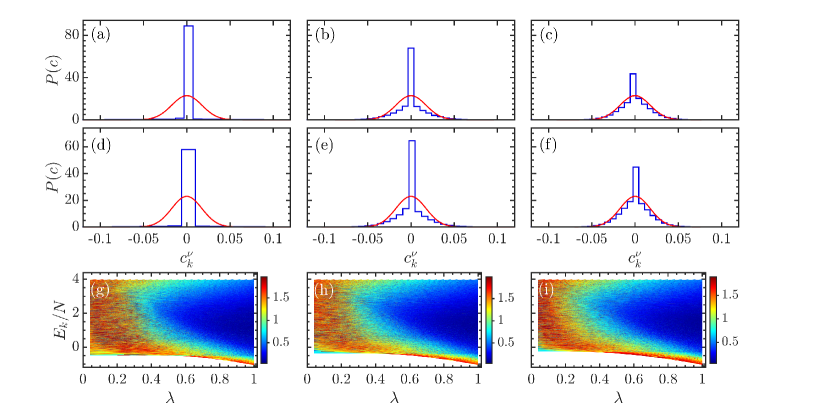
Figure 4: Panels (a)-(f): Histogramas of the coefficients $c_{k}^{\nu}$ of eigenstates with energy $E_{k}/N\in[1.75,2.25]$, in the Fock-Dicke basis. Each panel corresponds to different $(\kappa,\lambda)$ combinations: (a) $\kappa=0,\lambda=0$, (b) $\kappa=0,\lambda=0.5$, (c) $\kappa=0,\lambda=1$, (d) $\kappa=0.7,\lambda=0$, (e) $\kappa=0.7,\lambda=0.5$, and (f) $\kappa=0.7,\lambda=1$. The red solid line in each panel denotes the Gaussian distribution in Eq. (13). Panels (g)-(i): Kullback-Leibler divergence $D_{KL}$ [cf. Eq. (14)] as a function of rescaled energy $E_{k}/N$ and $\lambda$ for $\kappa=0$ (g), $\kappa=0.5$ (h), and $\kappa=1$ (i). Other parameters: $\omega=\omega_{0}=1$ and $N=2j=40$. All quantities are dimensionless.

A more stringent analysis of the effect of the atomic interaction is made with the average level spacing ratio, defined as

$$\langle r\rangle=\int_{0}^{1}rP(r)dr.$$ (11)

It takes the value $\langle r\rangle_{Poi}=2\ln 2-1\approx 0.386$ for integrable systems with $P(r)=P_{Poi}(r)$, while for chaotic systems with $P(r)=P_{GOE}(r)$, one has $\langle r\rangle_{GOE}=4-2\sqrt{3}\approx 0.536$. Hence, $\langle r\rangle$ acts as a detector to diagnose whether the studied system is in the integrable or chaotic regime and has been widely used to track the crossover from integrability to chaos.

Fig. 3(g) demonstrates $\langle r\rangle$ as a function of $\lambda$ for three different values $\kappa$. We see that, regardless of the value of $\kappa$, the transition from integrability to chaos is well captured by the behavior of $\langle r\rangle$, which varies from $\langle r\rangle_{Poi}$ to $\langle r\rangle_{GOE}$ with increasing $\lambda$. We further observe that the chaotic phase is robust with respect to variation of $\kappa$, but the integrable phase exhibits a strong dependence on $\kappa$. For the integrable phase with smaller values of $\lambda$, we find that increasing $\kappa$ gives rise to an increase of $\langle r\rangle$. As a consequence, the location of transition to chaos can be varied by the atomic intraction. This effect is more clearly observed in Fig. 3(h) where the evolves of $\langle r\rangle$ as a function of $\kappa$ and $\lambda$ has been illustrated. Again, we define the boundary of chaotic region by the condition $\langle r\rangle\geq\langle r\rangle_{c}=0.48$, meaning that the region with value $\langle r\rangle\geq 0.48$ is considered as chaos. We have checked that our main result still holds for other choices of $\langle r\rangle_{c}$, as long as $\langle r\rangle_{c}\in(0.45,0.5)$. The green line in Fig. 3(h) denotes the obtained boundary of chaos. As expected, the behavior of the boundary line confirms the extension of the chaotic region to lower values of $\lambda$ as $\kappa$ increases.

4 Structure of eigenstates

The onset of chaos also bears a remarkable change in the structure of eigenstates. In this section we explore the impact of atomic interaction on the transition to chaos by investigating the variation in the structure of eigenstates.

It is known that the eigenstates of chaotic systems are uncorrelated and are well described by random matrix theory (RMT) Borgonovi et al. (2016); Berry (1977); Porter and Thomas (1956); Mehta (2004). For the model studied in this work, one can expect that in the chaotic phase the eigenstates of the model will have the same structure as those of random GOE matrices. The GOE eigenstates are fully delocalized random vectors with real components consist of independent Gaussian random numbers. Hence, the deviation of eigenvector structure from Gaussian behavior is an alternative benchmark to certify quantum chaos Izrailev (1990); Haake and Życzkowski (1990); Zyczkowski (1990); Leboeuf and Voros (1990); Wang and Robnik (2021).

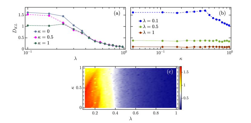
Figure 5: (a) KL divergence $D_{KL}$ (14) as a function of $\lambda$ for several $\kappa$ values. (b) $D_{KL}$ as a function of $\kappa$ for several coupling strengths $\lambda$. (c) Color scaled plot of $D_{KL}$ in the $\kappa-\lambda$ plane. In all panels, the coefficients distribution $P(c)$ is obtained from the eigenstates with energies $E_{k}/N\in[1.75,2.25]$. Other parameters: $\omega=\omega_{0}=1$ and $N=2j=40$. All quantities are dimensionless.

The analysis of the structure of eigenstates requires expansion of the eigenstates in a chosen basis. The choice of basis is usually decided by the physical problem and the system under consideration. Here, we use the Fock-Dicke basis, $\{|n,m\rangle\}$, which are the eigenstates of $a^{\dagger}a$ and $J_{z}$, as mentioned in Sec. 2. The decomposition of the $k$th eigenstate, $|k\rangle$, of the Hamiltonian (1) in the selected basis is given by

$$|k\rangle=\sum_{\nu=1}^{\mathcal{D}}c_{k}^{\nu}|\nu\rangle,$$ (12)

where $|\nu\rangle=|n,m\rangle$, $\mathcal{D}$ is the dimension of the Hilbert space, and $c_{k}^{\nu}=\langle\nu|k\rangle$ are the $k$th eigenstate components in the basis $\{|\nu\rangle\}$, satisfying the normalization condition $\sum_{\nu}|c_{k}^{\nu}|^{2}=1$. The characterizations of the eigenstate structure are provided by the statistical properties of eigenstate coefficients $\{c_{k}^{\nu}\}$.

To analyze the fingerprint of chaos in the properties of the eigenstates of $H$ in Eq. (1), as well as to examine whether the atomic interaction has effect on the eigenstate structure, we explore the coefficients distribution in comparison with the corresponding GOE result. As mentioned above, the eigenstates for the chaotic systems with real and symmetric $\mathcal{D}$-dimensional Hamiltonian matrices are consistent with the GOE eigenstates. The components of a GOE eigenstate, $\{c_{\nu}\}$, are random numbers that are uniformly distributed on a unit sphere with dimension $\mathcal{D}-1$. In the limit $\mathcal{D}\gg 1$, the dependence between components vanishes and the distribution of components can be well described by a Gaussian distribution with zero mean and variance $1/\mathcal{D}$ Brody et al. (1981); Torres-Herrera et al. (2016); Bäcker et al. (2019); Nakerst and Haque (2022),

$$P_{GOE}(c)=\sqrt{\frac{\mathcal{D}}{2\pi}}e^{-\mathcal{D}c^{2}/2}.$$ (13)

In the chaotic systems, it has been known that the coefficients of the mid-spectrum eigenstates are distributed as near-Gaussian distribution Brody et al. (1981); Guhr et al. (1998); Khaymovich et al. (2019); Pausch et al. (2021); Beugeling et al. (2018), while the coefficients distribution for eigenstates of non-chaotic systems and the edge eigenstates of chaotic systems is significantly different from Gaussian distribution Beugeling et al. (2018); Luitz and Bar Lev (2016); Luitz et al. (2020). As increasing $\lambda$ leads to the onset of chaos in the model, one would expect that the distribution of mid-spectrum eigenstates coefficients shoud be turned from non-Gaussian into near-Gaussian.

Figs. 4(a)-4(f) show the evolution of the eigenstates coefficients distributions, denoted by $P(c)$, for several $(\kappa,\lambda)$ combinations, in comparsion with the Gaussian distribution provided by Eq. (13). We see that, regardless of the value of $\kappa$, the eigenstates coefficients distribution tends to Gaussian as $\lambda$ increases. The larger the value of $\lambda$ is, the higher the degree of chaos in the model, and, therefore, the closer the coefficients distribution to Gaussian, as expected. Another prominent feature, that is also independent of $\kappa$, observed in the behaviors of $P(c)$ is the larger peak around $c_{k}^{\nu}\sim 0$. Even in the most chaotic regime, $P(c)$ still exhibits a high peak near zero, as shown in Figs. 4(c) and 4(f). This excessive number of zero coefficients is mainly due to the mixed feature of the model. This means the regular and chaotic behavior coexist in the model for the considered parameters. Detailed analysis of the mixture of regular and chaotic behaviors in extended Dicke model is beyond the scope of the present work, we leave this investigation for a furture work.

Let us now turn to discuss how the atomic interaction $\kappa$ affects the eigenstate coefficients distribution. As evident from Figs. 4(a)-4(f), the presence of atomic interaction has almost no effect on the behavior of eigenstate coefficients distribution, but just a reduction of the hight of peak in the regular phase [compare Figs. 4(a) to 4(d)]. This implies that the impact of the atomic interaction on the structure of eigenstates is not as strong as on the eigenlevels.

To measure the difference between $P(c)$ and Gaussian distribution (13), we consider Kullback-Leibler (KL) divergence Kullback and Leibler (1951), which is commonly used to measure how close an observed distribution is to a predicted distribution. In our study, $P(c)$ and $P_{GOE}(c)$ are, respectively, identified as the observed and predicted distributions. Then, the KL divergence between them is given by

$$D_{KL}=\int_{c_{min}}^{c_{max}}P(c)\ln\left[\frac{P(c)}{P_{GOE}(c)}\right]dc,$$ (14)

where $c_{min}$ and $c_{max}$ denote respectively the minimum and maximum values in $\{c_{k}^{\nu}\}$. The KL divergence is non-negative, so that $D_{KL}\geq 0$, and it vanishes only when $P(c)=P_{GOE}(c)$. Qualitatively, a larger $D_{KL}$ value indicates a larger difference between $P(c)$ and $P_{GOE}(c)$.

In Figs. 4(g)-4(i), we plot the KL divergence for the extended Dicke model as a function of $E_{k}/N$ and $\lambda$ with $\kappa=\{0,0.5,1\}$. We see that the behaviors of $D_{KL}$ versus $E_{k}/N$ and $\lambda$ for different $\kappa$ values are very similar. As expected, the eigenstates in the non-chaotic phase $(\lambda\lesssim 0.45)$ and the eigenstates at the spectrum edge in the chaotic phase $(\lambda\gtrsim 0.5)$ have larger values of $D_{KL}$, suggesting that the corresponding coefficients distributions strongly deviate from Gaussian, as illustrated in Figs. 4(a) and 4(d) for integrable case. Here, it is worth pointing out that the infinite dimension of the Hilbert space for the extended Dicke model leads to its spectrum has only one edge, namely the ground state. On the other hand, the lower values of $D_{KL}$ for mid-spectrum eigenstates in the chaotic phase imply that their coefficients distributions are closer to Gaussian, as shown in Figs. 4(c) and 4(f). The similarity between behaviors of $D_{KL}$ observed in the bottom row of Fig. (4) prompts a more detailed investigation of the impact of the atomic interaction on the eigenstate coefficient distribution.

To determine whether the eigenstate coefficients distribution is robust with respect to the variation of the atomic interaction $\kappa$, we calculate $D_{KL}$ for the mid-spectrum eigenstates with energies $E_{k}/N\in[1.75,2.25]$. The final result for various cases is shown in Fig. 5. The evolution of $D_{KL}$ as a function of $\lambda$ for different values of $\kappa$ is plotted in Fig. 5(a). One can see that the behavior of $D_{KL}$ for different $\kappa$ is very similar. The KL divergence varies slowly for smaller $\lambda$ until $\lambda\approx 0.25$, after which it rapidly decreases to small values as the coupling strength is increased beyond $\lambda_{c}\approx 0.5$. The change of $D_{KL}$ behavior is a manifestation of the transition to chaos resulting from the reduction of eigenstates correlation with increasing $\lambda$. We also observe that the dependence of $D_{KL}$ on $\kappa$ in the integrable phase is very different from that of chaotic phase. The explicit dependence of $D_{KL}$ on $\kappa$ for several values of $\lambda$ is shown in Fig. 5(b). As expected from Fig. 5(a), in the chaotic regime with $\lambda\gtrsim 0.5$, $D_{KL}$ is independent of $\kappa$, whereas the KL divergence strongly depends on the atomic interaction for the cases of smaller $\lambda$. Overall, the KL divergence decreases with increasing $\kappa$ in the integrable regime. This indicates that the proximity of the eigenstate coefficients distribution to the Gaussian distribution can be improved by the atomic interaction. Therefore, the atomic interaction can vary the degree of chaos in the extended Dicke model, in agreement with the results obtained from eigenvalue statistics. An overall evolution of $D_{KL}$ as a function of $\kappa$ and $\lambda$ is depicted in Fig. 5(c). We see that the chaotic region remains almost unchanged as $\kappa$ increases, in contrast to the extension behavior revealed by the eigenvalue-based detectors of quantum chaos [see Figs. 2(b), 2(d), and 3(h)]. This suggests that the level repulsion is more sensitive to the effect of atomic interaction than the structure of eigenstates.

5 Conclusions

In this article we have performed a detailed analysis of quantum chaotic characters of the extended Dicke model through the statistical properties of eigenvalues and eigenstates. The presence of interaction between atoms in the model further allows us to explore the dependence of chaotic properties of the model on the atomic interaction. It has been shown that the integrability-to-chaos transition of the original Dicke model as a function of the atom-field coupling is amplified by the interatomic interaction.

We have demonstrated that as the model moves from regular phase to chaotic phase, both the level spacing and level spacing ratio distributions undergo a crossover from Poisson to Wigner distribution, regardless of the strength of atomic interaction. However, the presence of atomic interaction can lead to a notable deviation of level spacing and spacing ratio distributions from Poisson distribution. To quantify this deviation and to measure the degree of chaos in the model, we consider three different chaos indictors to probe the transition from integrablity to chaos. All of these indicators are complementary to each other and are able to capture the crossover from Poisson to Wigner for both level spacing and level spacing ratio distributions. We have also shown that the behaviors of these indicators as a function of control parameters are very similar. In particular, we found that the degree of chaos of the model can be controlled by tuning the strength of atomic interaction. This result highlights the role of interaction in the development of chaos in quantum many-body systems and opens up the possiblity to tune the degree of chaos in the extended Dicke model.

Further quantum chaotic signatures showing how the atomic interaction affects the degree of chaos in the extended Dicke model are unveiled in the structure of the eigenstates. To analyze the eigenstate structure, we expand each eigenstate in the Fock-Dicke basis and focus on the expansion coefficients distribution for mid-spectrum eigenstates. For fully chaotic systems with Hamitonian from GOE, such distribution is well described by Gaussian distribution. We have shown that the transition to chaos can be detected by the deviation of coefficients distribution from Gaussian distribution. However, we note that even within the chaotic phase, the coefficients distribution is still different from Gaussian, indicating the existence of correlations between them. By using the KL divergence to measure the distance between the coefficients distribution and Gaussian distribution, we have illustrated that the onset of chaos corresponds to the rapid decrease in the behavior of KL divergence as a function of coupling strength. Although the atomic interaction leads to the decrease of KL divergence in the regular phase, the transition to chaos revealed by KL divergence is almost independent of atomic interaction. This is different from the results obtained by the eigenvalue-based chaos indicators and implies that unlike the eigenlevels, the eigenstate structure is robust with respect to the change of atomic interaction.

A nutural extension of the present work is to investigate the dynamical role played by the atomic interaction in the development of chaos. It would also be interesting to analyze the effect of atomic interaction on the level of chaoticity through the long-range spectral correlations, which can be detected by the spectral form factor Haake (2010). In addition, understanding the emergence of chaos and the impact of atomic interaction from the dynamics of the classical counterpart of the model would be another interesting topic. Very recently, the critical phenomena in the extended Dicke model have been thoroughly analyzed in this direction Herrera Romero et al. (2022). Finally, we would like to mention that a direct demonstration of level spacing distribution in an ultracold-atom system has been realized in a recent experiment Frisch et al. (2014). Hence, we expect that the spectral statistics of our studied extended Dicke model can be verified by the state-of-the-art experimental platforms.

This research was funded by the Slovenian Research Agency (ARRS) under the grant number J1-9112. Q. W. acknowledges support from the National Science Foundation of China under grant number 11805165, Zhejiang Provincial Nature Science Foundation under grant number LY20A050001.

Not applicable.

Not applicable.

Not applicable.

The authors declare no conflict of interest.

References

yes

References

- Altland and Haake (2012) Altland, A.; Haake, F. Quantum Chaos and Effective Thermalization. Phys. Rev. Lett. 2012, 108, 073601. doi:\changeurlcolorblack10.1103/PhysRevLett.108.073601.
- D’Alessio et al. (2016) D’Alessio, L.; Kafri, Y.; Polkovnikov, A.; Rigol, M. From quantum chaos and eigenstate thermalization to statistical mechanics and thermodynamics. Adv. Phys. 2016, 65, 239–362. doi:\changeurlcolorblack10.1080/00018732.2016.1198134.
- Borgonovi et al. (2016) Borgonovi, F.; Izrailev, F.; Santos, L.; Zelevinsky, V. Quantum chaos and thermalization in isolated systems of interacting particles. Phys. Rep. 2016, 626, 1–58. doi:\changeurlcolorblackhttps://doi.org/10.1016/j.physrep.2016.02.005.
- Nandkishore and Huse (2015) Nandkishore, R.; Huse, D.A. Many-Body Localization and Thermalization in Quantum Statistical Mechanics. Ann. Rev. Condens. Matter Phys. 2015, 6, 15–38. doi:\changeurlcolorblack10.1146/annurev-conmatphys-031214-014726.
- Deutsch (2018) Deutsch, J.M. Eigenstate thermalization hypothesis. Rep. Prog. Phys. 2018, 81, 082001. doi:\changeurlcolorblack10.1088/1361-6633/aac9f1.
- Chan et al. (2018) Chan, A.; De Luca, A.; Chalker, J.T. Solution of a Minimal Model for Many-Body Quantum Chaos. Phys. Rev. X 2018, 8, 041019. doi:\changeurlcolorblack10.1103/PhysRevX.8.041019.
- Garcia-March et al. (2018) Garcia-March, M.A.; van Frank, S.; Bonneau, M.; Schmiedmayer, J.; Lewenstein, M.; Santos, L.F. Relaxation, chaos, and thermalization in a three-mode model of a Bose–Einstein condensate. New Journal of Physics 2018, 20, 113039. doi:\changeurlcolorblack10.1088/1367-2630/aaed68.
- Friedman et al. (2019) Friedman, A.J.; Chan, A.; De Luca, A.; Chalker, J.T. Spectral Statistics and Many-Body Quantum Chaos with Conserved Charge. Phys. Rev. Lett. 2019, 123, 210603. doi:\changeurlcolorblack10.1103/PhysRevLett.123.210603.
- Ray et al. (2020) Ray, S.; Cohen, D.; Vardi, A. Chaos-induced breakdown of Bose-Hubbard modeling. Phys. Rev. A 2020, 101, 013624. doi:\changeurlcolorblack10.1103/PhysRevA.101.013624.
- Rautenberg and Gärttner (2020) Rautenberg, M.; Gärttner, M. Classical and quantum chaos in a three-mode bosonic system. Phys. Rev. A 2020, 101, 053604. doi:\changeurlcolorblack10.1103/PhysRevA.101.053604.
- Kobrin et al. (2021) Kobrin, B.; Yang, Z.; Kahanamoku-Meyer, G.D.; Olund, C.T.; Moore, J.E.; Stanford, D.; Yao, N.Y. Many-Body Chaos in the Sachdev-Ye-Kitaev Model. Phys. Rev. Lett. 2021, 126, 030602. doi:\changeurlcolorblack10.1103/PhysRevLett.126.030602.
- Fogarty et al. (2021) Fogarty, T.; García-March, M.Á.; Santos, L.F.; Harshman, N.L. Probing the edge between integrability and quantum chaos in interacting few-atom systems. Quantum 2021, 5, 486. doi:\changeurlcolorblack10.22331/q-2021-06-29-486.
- Wittmann W. et al. (2022) Wittmann W., K.; Castro, E.R.; Foerster, A.; Santos, L.F. Interacting bosons in a triple well: Preface of many-body quantum chaos. Phys. Rev. E 2022, 105, 034204. doi:\changeurlcolorblack10.1103/PhysRevE.105.034204.
- Maldacena et al. (2016) Maldacena, J.; Shenker, S.H.; Stanford, D. A bound on chaos. J. High Energy Phys. 2016, 2016, 106. doi:\changeurlcolorblack10.1007/JHEP08(2016)106.
- Stanford (2016) Stanford, D. Many-body chaos at weak coupling. J. High Energy Phys. 2016, 2016, 9. doi:\changeurlcolorblack10.1007/JHEP10(2016)009.
- Magán (2018) Magán, J.M. Black holes, complexity and quantum chaos. J. High Energy Phys. 2018, 2018, 43. doi:\changeurlcolorblack10.1007/JHEP09(2018)043.
- Jahnke (2019) Jahnke, V. Recent Developments in the Holographic Description of Quantum Chaos. Adv. High Energy Phys. 2019, 2019, 9632708. doi:\changeurlcolorblack10.1155/2019/9632708.
- Ali et al. (2020) Ali, T.; Bhattacharyya, A.; Haque, S.S.; Kim, E.H.; Moynihan, N.; Murugan, J. Chaos and complexity in quantum mechanics. Phys. Rev. D 2020, 101, 026021. doi:\changeurlcolorblack10.1103/PhysRevD.101.026021.
- Rabinovici et al. (2021) Rabinovici, E.; Sánchez-Garrido, A.; Shir, R.; Sonner, J. Operator complexity: a journey to the edge of Krylov space. J. High Energy Phys. 2021, 2021, 62.
- Schack and Caves (1996) Schack, R.; Caves, C.M. Information-theoretic characterization of quantum chaos. Phys. Rev. E 1996, 53, 3257–3270. doi:\changeurlcolorblack10.1103/PhysRevE.53.3257.
- Vidmar and Rigol (2017) Vidmar, L.; Rigol, M. Entanglement Entropy of Eigenstates of Quantum Chaotic Hamiltonians. Phys. Rev. Lett. 2017, 119, 220603. doi:\changeurlcolorblack10.1103/PhysRevLett.119.220603.
- Piga et al. (2019) Piga, A.; Lewenstein, M.; Quach, J.Q. Quantum chaos and entanglement in ergodic and nonergodic systems. Phys. Rev. E 2019, 99, 032213. doi:\changeurlcolorblack10.1103/PhysRevE.99.032213.
- Bertini et al. (2019) Bertini, B.; Kos, P.; Prosen, T.c.v. Entanglement Spreading in a Minimal Model of Maximal Many-Body Quantum Chaos. Phys. Rev. X 2019, 9, 021033. doi:\changeurlcolorblack10.1103/PhysRevX.9.021033.
- Lerose and Pappalardi (2020) Lerose, A.; Pappalardi, S. Bridging entanglement dynamics and chaos in semiclassical systems. Phys. Rev. A 2020, 102, 032404. doi:\changeurlcolorblack10.1103/PhysRevA.102.032404.
- Lantagne-Hurtubise et al. (2020) Lantagne-Hurtubise, E.; Plugge, S.; Can, O.; Franz, M. Diagnosing quantum chaos in many-body systems using entanglement as a resource. Phys. Rev. Research 2020, 2, 013254. doi:\changeurlcolorblack10.1103/PhysRevResearch.2.013254.
- Anand et al. (2021) Anand, N.; Styliaris, G.; Kumari, M.; Zanardi, P. Quantum coherence as a signature of chaos. Phys. Rev. Research 2021, 3, 023214. doi:\changeurlcolorblack10.1103/PhysRevResearch.3.023214.
- Hosur et al. (2016) Hosur, P.; Qi, X.L.; Roberts, D.A.; Yoshida, B. Chaos in quantum channels. Journal of High Energy Physics 2016, 2016, 4.
- Chenu et al. (2019) Chenu, A.; Molina-Vilaplana, J.; del Campo, A. Work Statistics, Loschmidt Echo and Information Scrambling in Chaotic Quantum Systems. Quantum 2019, 3, 127. doi:\changeurlcolorblack10.22331/q-2019-03-04-127.
- Prakash and Lakshminarayan (2020) Prakash, R.; Lakshminarayan, A. Scrambling in strongly chaotic weakly coupled bipartite systems: Universality beyond the Ehrenfest timescale. Phys. Rev. B 2020, 101, 121108. doi:\changeurlcolorblack10.1103/PhysRevB.101.121108.
- Balasubramanian et al. (2020) Balasubramanian, V.; DeCross, M.; Kar, A.; Parrikar, O. Quantum complexity of time evolution with chaotic Hamiltonians. Journal of High Energy Physics 2020, 2020, 134.
- Bhattacharyya et al. (2021a) Bhattacharyya, A.; Haque, S.S.; Kim, E.H. Complexity from the reduced density matrix: a new diagnostic for chaos. Journal of High Energy Physics 2021, 2021, 28.
- Bhattacharyya et al. (2021b) Bhattacharyya, A.; Chemissany, W.; Haque, S.S.; Murugan, J.; Yan, B. The Multi-faceted Inverted Harmonic Oscillator: Chaos and Complexity. SciPost Phys. Core 2021, 4, 2. doi:\changeurlcolorblack10.21468/SciPostPhysCore.4.1.002.
- Parker et al. (2019) Parker, D.E.; Cao, X.; Avdoshkin, A.; Scaffidi, T.; Altman, E. A Universal Operator Growth Hypothesis. Phys. Rev. X 2019, 9, 041017. doi:\changeurlcolorblack10.1103/PhysRevX.9.041017.
- Dymarsky and Gorsky (2020) Dymarsky, A.; Gorsky, A. Quantum chaos as delocalization in Krylov space. Phys. Rev. B 2020, 102, 085137. doi:\changeurlcolorblack10.1103/PhysRevB.102.085137.
- Caputa et al. (2022) Caputa, P.; Magan, J.M.; Patramanis, D. Geometry of Krylov complexity. Phys. Rev. Research 2022, 4, 013041. doi:\changeurlcolorblack10.1103/PhysRevResearch.4.013041.
- Bertini et al. (2021) Bertini, B.; Heidrich-Meisner, F.; Karrasch, C.; Prosen, T.; Steinigeweg, R.; Žnidarič, M. Finite-temperature transport in one-dimensional quantum lattice models. Rev. Mod. Phys. 2021, 93, 025003. doi:\changeurlcolorblack10.1103/RevModPhys.93.025003.
- Cvitanovic et al. (2005) Cvitanovic, P.; Artuso, R.; Mainieri, R.; Tanner, G.; Vattay, G.; Whelan, N.; Wirzba, A. Chaos: classical and quantum. ChaosBook. org (Niels Bohr Institute, Copenhagen 2005) 2005, 69, 25.
- Schuster and Just (2006) Schuster, H.G.; Just, W. Deterministic chaos: an introduction; John Wiley & Sons, 2006.
- Bohigas et al. (1984) Bohigas, O.; Giannoni, M.J.; Schmit, C. Characterization of Chaotic Quantum Spectra and Universality of Level Fluctuation Laws. Phys. Rev. Lett. 1984, 52, 1–4. doi:\changeurlcolorblack10.1103/PhysRevLett.52.1.
- Stöckmann (1999) Stöckmann, H.J. Quantum Chaos: An Introduction; Cambridge University Press, 1999. doi:\changeurlcolorblack10.1017/CBO9780511524622.
- Haake (2010) Haake, F. Quantum Signatures of Chaos; Springer, Berlin Heidelberg, 2010.
- Zyczkowski (1990) Zyczkowski, K. Indicators of quantum chaos based on eigenvector statistics. J. Phys. A 1990, 23, 4427.
- Emerson et al. (2002) Emerson, J.; Weinstein, Y.S.; Lloyd, S.; Cory, D.G. Fidelity Decay as an Efficient Indicator of Quantum Chaos. Phys. Rev. Lett. 2002, 89, 284102. doi:\changeurlcolorblack10.1103/PhysRevLett.89.284102.
- Rozenbaum et al. (2017) Rozenbaum, E.B.; Ganeshan, S.; Galitski, V. Lyapunov Exponent and Out-of-Time-Ordered Correlator’s Growth Rate in a Chaotic System. Phys. Rev. Lett. 2017, 118, 086801. doi:\changeurlcolorblack10.1103/PhysRevLett.118.086801.
- García-Mata et al. (2018) García-Mata, I.; Saraceno, M.; Jalabert, R.A.; Roncaglia, A.J.; Wisniacki, D.A. Chaos Signatures in the Short and Long Time Behavior of the Out-of-Time Ordered Correlator. Phys. Rev. Lett. 2018, 121, 210601. doi:\changeurlcolorblack10.1103/PhysRevLett.121.210601.
- Chen and Ludwig (2018) Chen, X.; Ludwig, A.W.W. Universal spectral correlations in the chaotic wave function and the development of quantum chaos. Phys. Rev. B 2018, 98, 064309. doi:\changeurlcolorblack10.1103/PhysRevB.98.064309.
- Kos et al. (2018) Kos, P.; Ljubotina, M.; Prosen, T.c.v. Many-Body Quantum Chaos: Analytic Connection to Random Matrix Theory. Phys. Rev. X 2018, 8, 021062. doi:\changeurlcolorblack10.1103/PhysRevX.8.021062.
- Bertini et al. (2018) Bertini, B.; Kos, P.; Prosen, T.c.v. Exact Spectral Form Factor in a Minimal Model of Many-Body Quantum Chaos. Phys. Rev. Lett. 2018, 121, 264101. doi:\changeurlcolorblack10.1103/PhysRevLett.121.264101.
- Gietka et al. (2019) Gietka, K.; Chwedeńczuk, J.; Wasak, T.; Piazza, F. Multipartite entanglement dynamics in a regular-to-ergodic transition: Quantum Fisher information approach. Phys. Rev. B 2019, 99, 064303. doi:\changeurlcolorblack10.1103/PhysRevB.99.064303.
- Xu et al. (2020) Xu, T.; Scaffidi, T.; Cao, X. Does Scrambling Equal Chaos? Phys. Rev. Lett. 2020, 124, 140602. doi:\changeurlcolorblack10.1103/PhysRevLett.124.140602.
- Cao et al. (2021) Cao, Z.; Xu, Z.; del Campo, A. Probing quantum chaos in multipartite systems. arXiv e-prints 2021, p. arXiv:2111.12475, [arXiv:quant-ph/2111.12475].
- Zonnios et al. (2022) Zonnios, M.; Levinsen, J.; Parish, M.M.; Pollock, F.A.; Modi, K. Signatures of Quantum Chaos in an Out-of-Time-Order Tensor. Phys. Rev. Lett. 2022, 128, 150601. doi:\changeurlcolorblack10.1103/PhysRevLett.128.150601.
- Raúl González Alonso et al. (2022) Raúl González Alonso, J.; Shammah, N.; Ahmed, S.; Nori, F.; Dressel, J. Diagnosing quantum chaos with out-of-time-ordered-correlator quasiprobability in the kicked-top model. arXiv e-prints 2022, p. arXiv:2201.08175, [arXiv:quant-ph/2201.08175].
- Joshi et al. (2022) Joshi, L.K.; Elben, A.; Vikram, A.; Vermersch, B.; Galitski, V.; Zoller, P. Probing Many-Body Quantum Chaos with Quantum Simulators. Phys. Rev. X 2022, 12, 011018. doi:\changeurlcolorblack10.1103/PhysRevX.12.011018.
- Lozej et al. (2022) Lozej, Č.; Lukman, D.; Robnik, M. Phenomenology of quantum eigenstates in mixed-type systems: lemon billiards with complex phase space structure. arXiv e-prints 2022, p. arXiv:2207.07197, [arXiv:nlin.CD/2207.07197].
- Abanin et al. (2019) Abanin, D.A.; Altman, E.; Bloch, I.; Serbyn, M. Colloquium: Many-body localization, thermalization, and entanglement. Rev. Mod. Phys. 2019, 91, 021001. doi:\changeurlcolorblack10.1103/RevModPhys.91.021001.
- Turner et al. (2018) Turner, C.J.; Michailidis, A.A.; Abanin, D.A.; Serbyn, M.; Papić, Z. Weak ergodicity breaking from quantum many-body scars. Nature Physics 2018, 14, 745–749.
- Sinha and Sinha (2020) Sinha, S.; Sinha, S. Chaos and Quantum Scars in Bose-Josephson Junction Coupled to a Bosonic Mode. Phys. Rev. Lett. 2020, 125, 134101. doi:\changeurlcolorblack10.1103/PhysRevLett.125.134101.
- Turner et al. (2021) Turner, C.J.; Desaules, J.Y.; Bull, K.; Papić, Z. Correspondence Principle for Many-Body Scars in Ultracold Rydberg Atoms. Phys. Rev. X 2021, 11, 021021. doi:\changeurlcolorblack10.1103/PhysRevX.11.021021.
- Mondragon-Shem et al. (2021) Mondragon-Shem, I.; Vavilov, M.G.; Martin, I. Fate of Quantum Many-Body Scars in the Presence of Disorder. PRX Quantum 2021, 2, 030349. doi:\changeurlcolorblack10.1103/PRXQuantum.2.030349.
- Serbyn et al. (2021) Serbyn, M.; Abanin, D.A.; Papić, Z. Quantum many-body scars and weak breaking of ergodicity. Nature Physics 2021, 17, 675–685.
- Kloc et al. (2017) Kloc, M.; Stránský, P.; Cejnar, P. Quantum phases and entanglement properties of an extended Dicke model. Annals of Physics 2017, 382, 85–111. doi:\changeurlcolorblackhttps://doi.org/10.1016/j.aop.2017.04.005.
- Rodriguez et al. (2018) Rodriguez, J.P.J.; Chilingaryan, S.A.; Rodríguez-Lara, B.M. Critical phenomena in an extended Dicke model. Phys. Rev. A 2018, 98, 043805. doi:\changeurlcolorblack10.1103/PhysRevA.98.043805.
- Guerra et al. (2020) Guerra, C.A.E.; Mahecha-Gómez, J.; Hirsch, J.G. Quantum phase transition and Berry phase in an extended Dicke model. The European Physical Journal D 2020, 74, 200.
- Herrera Romero et al. (2022) Herrera Romero, R.; Bastarrachea-Magnani, M.A.; Linares, R. Critical Phenomena in Light-Matter Systems with Collective Matter Interactions. Entropy 2022, 24. doi:\changeurlcolorblack10.3390/e24091198.
- Dicke (1954) Dicke, R.H. Coherence in Spontaneous Radiation Processes. Phys. Rev. 1954, 93, 99–110. doi:\changeurlcolorblack10.1103/PhysRev.93.99.
- Emary and Brandes (2003) Emary, C.; Brandes, T. Chaos and the quantum phase transition in the Dicke model. Phys. Rev. E 2003, 67, 066203. doi:\changeurlcolorblack10.1103/PhysRevE.67.066203.
- Wang and Robnik (2020) Wang, Q.; Robnik, M. Statistical properties of the localization measure of chaotic eigenstates in the Dicke model. Phys. Rev. E 2020, 102, 032212. doi:\changeurlcolorblack10.1103/PhysRevE.102.032212.
- Bastarrachea-Magnani et al. (2015) Bastarrachea-Magnani, M.A.; del Carpio, B.L.; Lerma-Hernández, S.; Hirsch, J.G. Chaos in the Dicke model: quantum and semiclassical analysis. Physica Scripta 2015, 90, 068015. doi:\changeurlcolorblack10.1088/0031-8949/90/6/068015.
- Bastarrachea-Magnani et al. (2016) Bastarrachea-Magnani, M.A.; López-del Carpio, B.; Chávez-Carlos, J.; Lerma-Hernández, S.; Hirsch, J.G. Delocalization and quantum chaos in atom-field systems. Phys. Rev. E 2016, 93, 022215. doi:\changeurlcolorblack10.1103/PhysRevE.93.022215.
- Robles Robles et al. (2015) Robles Robles, R.A.; Chilingaryan, S.A.; Rodríguez-Lara, B.M.; Lee, R.K. Ground state in the finite Dicke model for interacting qubits. Phys. Rev. A 2015, 91, 033819. doi:\changeurlcolorblack10.1103/PhysRevA.91.033819.
- Cejnar et al. (2011) Cejnar, P.; Stránský, P.; Macek, M. Regular and Chaotic Collective Modes in Nuclei. Nuclear Physics News 2011, 21, 22–27, [https://doi.org/10.1080/10619127.2011.629919]. doi:\changeurlcolorblack10.1080/10619127.2011.629919.
- Chávez-Carlos et al. (2019) Chávez-Carlos, J.; López-del Carpio, B.; Bastarrachea-Magnani, M.A.; Stránský, P.; Lerma-Hernández, S.; Santos, L.F.; Hirsch, J.G. Quantum and Classical Lyapunov Exponents in Atom-Field Interaction Systems. Phys. Rev. Lett. 2019, 122, 024101. doi:\changeurlcolorblack10.1103/PhysRevLett.122.024101.
- Rodríguez-Lara and Lee (2011) Rodríguez-Lara, B.M.; Lee, R.K. Classical dynamics of a two-species condensate driven by a quantum field. Phys. Rev. E 2011, 84, 016225. doi:\changeurlcolorblack10.1103/PhysRevE.84.016225.
- Berry and Tabor (1977) Berry, M.V.; Tabor, M. Level clustering in the regular spectrum. Proc. R. Soc. A 1977, 356, 375–394. doi:\changeurlcolorblack10.1098/rspa.1977.0140.
- Jacquod and Shepelyansky (1997) Jacquod, P.; Shepelyansky, D.L. Emergence of Quantum Chaos in Finite Interacting Fermi Systems. Phys. Rev. Lett. 1997, 79, 1837–1840. doi:\changeurlcolorblack10.1103/PhysRevLett.79.1837.
- Brody et al. (1981) Brody, T.A.; Flores, J.; French, J.B.; Mello, P.A.; Pandey, A.; Wong, S.S.M. Random-matrix physics: spectrum and strength fluctuations. Rev. Mod. Phys. 1981, 53, 385–479. doi:\changeurlcolorblack10.1103/RevModPhys.53.385.
- Guhr et al. (1998) Guhr, T.; Müller–Groeling, A.; Weidenmüller, H.A. Random-matrix theories in quantum physics: common concepts. Physics Reports 1998, 299, 189–425. doi:\changeurlcolorblackhttps://doi.org/10.1016/S0370-1573(97)00088-4.
- Oganesyan and Huse (2007) Oganesyan, V.; Huse, D.A. Localization of interacting fermions at high temperature. Phys. Rev. B 2007, 75, 155111. doi:\changeurlcolorblack10.1103/PhysRevB.75.155111.
- Atas et al. (2013a) Atas, Y.Y.; Bogomolny, E.; Giraud, O.; Roux, G. Distribution of the Ratio of Consecutive Level Spacings in Random Matrix Ensembles. Phys. Rev. Lett. 2013, 110, 084101. doi:\changeurlcolorblack10.1103/PhysRevLett.110.084101.
- Atas et al. (2013b) Atas, Y.Y.; Bogomolny, E.; Giraud, O.; Vivo, P.; Vivo, E. Joint probability densities of level spacing ratios in random matrices. Journal of Physics A: Mathematical and Theoretical 2013, 46, 355204. doi:\changeurlcolorblack10.1088/1751-8113/46/35/355204.
- Giraud et al. (2022) Giraud, O.; Macé, N.; Vernier, E.; Alet, F. Probing Symmetries of Quantum Many-Body Systems through Gap Ratio Statistics. Phys. Rev. X 2022, 12, 011006. doi:\changeurlcolorblack10.1103/PhysRevX.12.011006.
- Berry (1977) Berry, M.V. Regular and irregular semiclassical wavefunctions. J. Phys. A 1977, 10, 2083–2091. doi:\changeurlcolorblack10.1088/0305-4470/10/12/016.
- Porter and Thomas (1956) Porter, C.E.; Thomas, R.G. Fluctuations of Nuclear Reaction Widths. Phys. Rev. 1956, 104, 483–491. doi:\changeurlcolorblack10.1103/PhysRev.104.483.
- Mehta (2004) Mehta, M.L. Random matrices; Elsevier, 2004.
- Izrailev (1990) Izrailev, F.M. Simple models of quantum chaos: Spectrum and eigenfunctions. Phys. Rep. 1990, 196, 299–392. doi:\changeurlcolorblackhttps://doi.org/10.1016/0370-1573(90)90067-C.
- Haake and Życzkowski (1990) Haake, F.; Życzkowski, K. Random-matrix theory and eigenmodes of dynamical systems. Phys. Rev. A 1990, 42, 1013–1016. doi:\changeurlcolorblack10.1103/PhysRevA.42.1013.
- Leboeuf and Voros (1990) Leboeuf, P.; Voros, A. Chaos-revealing multiplicative representation of quantum eigenstates. J. Phys. A: Mathematical and General 1990, 23, 1765–1774. doi:\changeurlcolorblack10.1088/0305-4470/23/10/017.
- Wang and Robnik (2021) Wang, Q.; Robnik, M. Multifractality in Quasienergy Space of Coherent States as a Signature of Quantum Chaos. Entropy 2021, 23. doi:\changeurlcolorblack10.3390/e23101347.
- Torres-Herrera et al. (2016) Torres-Herrera, E.J.; Karp, J.; Távora, M.; Santos, L.F. Realistic Many-Body Quantum Systems vs. Full Random Matrices: Static and Dynamical Properties. Entropy 2016, 18. doi:\changeurlcolorblack10.3390/e18100359.
- Bäcker et al. (2019) Bäcker, A.; Haque, M.; Khaymovich, I.M. Multifractal dimensions for random matrices, chaotic quantum maps, and many-body systems. Phys. Rev. E 2019, 100, 032117. doi:\changeurlcolorblack10.1103/PhysRevE.100.032117.
- Nakerst and Haque (2022) Nakerst, G.; Haque, M. Chaos in the three-site Bose-Hubbard model – classical vs quantum. arXiv e-prints 2022, p. arXiv:2203.09953, [arXiv:quant-ph/2203.09953].
- Khaymovich et al. (2019) Khaymovich, I.M.; Haque, M.; McClarty, P.A. Eigenstate Thermalization, Random Matrix Theory, and Behemoths. Phys. Rev. Lett. 2019, 122, 070601. doi:\changeurlcolorblack10.1103/PhysRevLett.122.070601.
- Pausch et al. (2021) Pausch, L.; Carnio, E.G.; Rodríguez, A.; Buchleitner, A. Chaos and Ergodicity across the Energy Spectrum of Interacting Bosons. Phys. Rev. Lett. 2021, 126, 150601. doi:\changeurlcolorblack10.1103/PhysRevLett.126.150601.
- Beugeling et al. (2018) Beugeling, W.; Bäcker, A.; Moessner, R.; Haque, M. Statistical properties of eigenstate amplitudes in complex quantum systems. Phys. Rev. E 2018, 98, 022204. doi:\changeurlcolorblack10.1103/PhysRevE.98.022204.
- Luitz and Bar Lev (2016) Luitz, D.J.; Bar Lev, Y. Anomalous Thermalization in Ergodic Systems. Phys. Rev. Lett. 2016, 117, 170404. doi:\changeurlcolorblack10.1103/PhysRevLett.117.170404.
- Luitz et al. (2020) Luitz, D.J.; Khaymovich, I.M.; Lev, Y.B. Multifractality and its role in anomalous transport in the disordered XXZ spin-chain. SciPost Phys. Core 2020, 2, 6. doi:\changeurlcolorblack10.21468/SciPostPhysCore.2.2.006.
- Kullback and Leibler (1951) Kullback, S.; Leibler, R.A. On Information and Sufficiency. Ann. Math. Stat. 1951, 22, 79–86.
- Frisch et al. (2014) Frisch, A.; Mark, M.; Aikawa, K.; Ferlaino, F.; Bohn, J.L.; Makrides, C.; Petrov, A.; Kotochigova, S. Quantum chaos in ultracold collisions of gas-phase erbium atoms. Nature 2014, 507, 475–479.