SaiT: Sparse Vision Transformers through Adaptive Token Pruning

Abstract

While vision transformers have achieved impressive results, effectively and efficiently accelerating these models can further boost performances. In this work, we propose a dense/sparse training framework to obtain a unified model, enabling weight sharing across various token densities. Thus one model offers a range of accuracy and throughput tradeoffs for different applications. Besides, we introduce adaptive token pruning to optimize the patch token sparsity based on the input image. In addition, we investigate knowledge distillation to enhance token selection capability in early transformer modules. Sparse adaptive image Transformer (SaiT) offers varying levels of model acceleration by merely changing the token sparsity on the fly. Specifically, SaiT reduces the computation complexity (FLOPs) by 39% - 43% and increases the throughput by 67% - 91% with less than 0.5% accuracy loss for various vision transformer models. Meanwhile, the same model also provides the zero accuracy drop option by skipping the sparsification step. SaiT achieves better accuracy and computation tradeoffs than state-of-the-art transformer and convolutional models.

1 Introduction

Even though Convolutional Neural Networks (CNNs) (Krizhevsky et al., 2012; He et al., 2016; Tan & Le, 2019) have fueled rapid development in the computer vision field, emerging studies on vision transformers show encouraging results, with some surpassing CNNs in a wide range of tasks such as classification (Dosovitskiy et al., 2021; Touvron et al., 2021a; Liu et al., 2021a), semantic segmentation (Cheng et al., 2021; Zheng et al., 2021) , and object detection (Carion et al., 2020; Li et al., 2022). To improve model efficiency, especially on edge devices, model compression techniques such as pruning (Han et al., 2015), quantization (Gong et al., 2014), and knowledge distillation (Hinton et al., 2015) have been widely used in CNNs. However, model acceleration/compression in vision transformers is still less explored. Additionally, these typical compression techniques – which usually lead to some accuracy loss – are not ideal for accuracy-sensitive applications.

For efficient and hardware-friendly model acceleration, we leverage the intrinsic structure of vision transformers, where input images are transformed into patch tokens before further processing. Patch tokens allow the vision transformer to process the entire image; however, the computation for the all-to-all attention is expensive. Token pruning is an effective approach to reduce computation and save memory. The essential number of patch tokens varies depending on the input image, since background patches often contribute little for correct classification. Some ’easy’ inputs require fewer patches and ’difficult’ inputs need more patches. Figure 1 shows that for ’easy’ inputs, such as the bird image on the upper left, around 20% of patches are sufficient for detection, whereas ’difficult’ inputs, such as the fishes on the lower right, require 53% token density. To save more computation based on the specifics of input images, we propose an adaptive token pruning strategy that dynamically adjusts the number of preserved tokens. This approach evaluates the importance (in probability) of each token based on the attention scores of the early transformer modules. Instead of selecting a fixed number of tokens, we accumulate a varying number of the most important tokens up to a probability mass threshold. As a result, this introduces no extra parameters and negligible computation, and thus its efficiency compares favorably with some prior works (Wang et al., 2021b; Rao et al., 2021).

In addition, we formulate a dense/sparse training framework to obtain a unified model which can flexibly adjust the tradeoff between accuracy and throughput on demand. Different computation savings are achieved by merely modifying the token density in the later transformer modules. Sharing the same weights throughout the transformer model, fully dense patch tokens preserve accuracy, but no model acceleration, while sparse tokens offer varying levels of acceleration in return for some accuracy drop. Therefore, different applications can share the same model and weights regardless of accuracy and throughput requirements. Consequently, this approach saves training cost and memory footprint by training and storing a single unified model instead of a series of different models.

To demonstrate the effectiveness of this approach, we deploy our proposed training framework and sparsification schemes on top of DeiT (Touvron et al., 2021a) and LVViT (Jiang et al., 2021). The resulting unified model, Sparse adaptive image Transformer (SaiT), offers different levels of sparsification and achieves 39% - 43% floating point operation (FLOP) reduction and 74-91% throughput gain with less than 0.5% accuracy loss. In summary, we present three major contributions of this work: 1) We formulate a dense/sparse training framework to obtain a unified model offering a range of accuracy and throughput tradeoffs; 2) We propose an adaptive pruning strategy to flexibly and dynamically adjust the token sparsity based on the input images; 3) We introduce knowledge distillation to improve the accuracy of early transformer modules in learning the token importance.

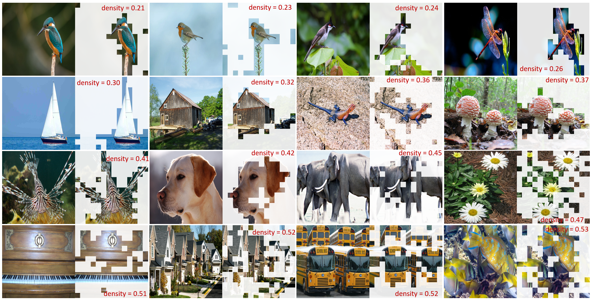
Figure 1: Visualization of the adaptive pruning based on the results from SaiT-S^†. Original image and sparsification results are presented next to each other. Based on the difficulties of the inputs, the densities of essential patch tokens dynamically change from 21% to 53%.

2 Related Work

Vision Transformers ViT (Dosovitskiy et al., 2021) is the first pure transformer based-model for image classification with results competitive to CNNs. However, the training of ViT requires a large private dataset JFT300M (Sun et al., 2017). To address this issue, DeiT (Touvron et al., 2021a) develops a training schedule with data augmentation, regularization, and knowledge distillation. Many subsequent variants  (Touvron et al., 2021b; Liu et al., 2021a; Chu et al., 2021; Jiang et al., 2021) of ViT and DeiT achieve promising performances, with some even surpassing CNN counterparts (He et al., 2016; Tan & Le, 2019; Radosavovic et al., 2020). Moreover, self-supervised vision transformers, such as DINO (Caron et al., 2021) and MAE (He et al., 2021), not only achieve impressive classification accuracy but also obtain useful feature representations for downstream tasks such as object detection and segmentation.

Efficient Vision Transformers To improve model efficiency and save computation, Wu et al. (2021b) and Jaegle et al. (2021) introduce new attention modules, while other works (Li et al., 2021b; Srinivas et al., 2021; Graham et al., 2021; Li et al., 2021a; Wu et al., 2021a; Xu et al., 2021; Guo et al., 2021) incorporate some convolutional layers into vision transformers. Following conventional model compression approaches, Liu et al. (2021b) apply post-training quantization in vision transformers, Chen et al. (2021b) study the sparsity via sparse subnetwork training, and Rao et al. (2021) implement a lightweight prediction module for hierarchical token pruning. Wang et al. (2021b) dynamically adjusts the number of patch tokens through cascading multiple transformers with confidence estimation modules. Liang et al. (2022) exploits the classification token to select attentive tokens without introducing extra parameters and fuse inattentive tokens through multiple stages for efficient inference.

Compared to prior works, our token pruning strategy is more efficient by leveraging the attention scores for one-stage adaptive pruning, with no extra parameters and negligible computation. Besides, the unified model from our dense/sparse training framework offers a range of accuracy and throughput tradeoffs for different applications.

3 SaiT

The proposed dense/sparse training framework and adaptive token pruning apply to general vision transformer architectures. To illustrate the ideas, we use DeiT (Touvron et al., 2021a) and LVViT (Jiang et al., 2021) as examples in this work. Both DeiT and LVViT use an embedding module to convert an input image into $N$ patch tokens. These $N$ patch tokens, along with the classification token $CLS$, go through a series of transformer modules/layers. The feature representation from the last transformer layer is used for the final classification. The key to the proposed approach is to enable early layers to effectively capture the importance of each token, in order to reduce computation in the later layers with sparse tokens.

3.1 Dense/sparse training framework

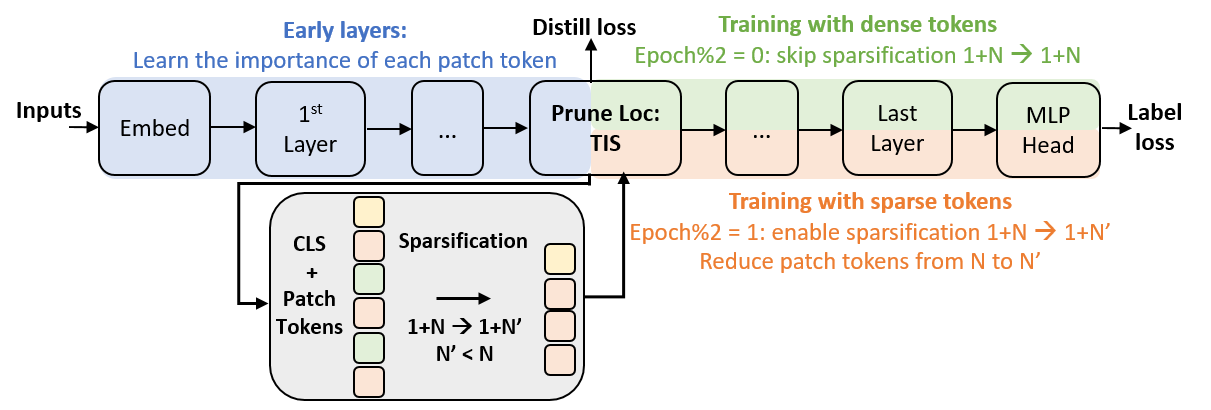
Figure 2: An overview of the dense/sparse training framework used in SaiT. Early layers (blue) learn the importance of each token. The attention scores at the prune-location are used to extract token importance score ($TIS$) and the token mask. Later layers are trained alternately with fully dense tokens (green) and sparse tokens (orange). Optionally, knowledge distillation from a teacher model enhances $TIS$ learning ability of early layers.

The overview of the dense/sparse training framework is in Figure 2 and Algorithm 1. Given an architecture with $L$ total transformer layers, the early layers ($l^{0}$ to $l^{P-1}$) learn to identify the importance of each patch token. At the designated pruning location ($l^{P}$), token importance scores ($TIS$) are extracted based on the attention scores, which are used for token selection and knowledge distillation. Later layers ($l^{P+1}$ to $l^{L-1}$) are trained on alternate epochs with $N$ fully dense patch tokens (without pruning) and $N^{\prime}$ sparse patch tokens (after pruning).

Algorithm 1 A General Training Framework used in SaiT

  Input: pretrained teacher model $W_{t}$, token pruning location $l^{P}$, distillation ratio $\beta$

  Initialize student weights $W_{s}$.

  for epoch $i=1$ to $T$ do

     Obtain the classification token $\overline{CLS}$ from the last layer of the teacher model

     Obtain student $TIS^{*P}$ and token mask $M$ at layer $l^{P}$,

     Calculate token distillation loss $L_{distill}=KL(TIS^{*P},\overline{CLS})$

     if $i\mod 2=0$ then

        Dense – skip token sparsification and use all the patch tokens after layer $l^{P}$

     else

        Sparse – prune tokens based on the token mask $M$ and use only sparse tokens after layer $l^{P}$

     end if

     Compute the label loss $L_{label}$ and total loss $L=L_{label}+\beta L_{distill}$

     Update student network

  end for

Dense/sparse alternate training This training schedule enables weight sharing between fully dense (unpruned) and sparse (pruned) patch tokens at layers $l^{P+1}$ to $l^{L-1}$, since the weights of transformer blocks are independent of the number of patch tokens. Moreover, it improves processing accuracy of later layer on sparse tokens as shown in the ablation study (Section 4.5). Besides, training with this framework preserves the model accuracy when skipping the sparsification. This is different from prior pruning models (Rao et al., 2021; Liang et al., 2022), which are unable to recover the original accuracy with dense tokens.

3.2 Token sparsification strategies

We leverage the attention scores to extract the Token Importance Score ($TIS$) for token sparsification during training and inference. For the token $n$, at the pruning layer $l^{P}$, $TIS$ is defined as:

$$TIS_{n}^{P}=\frac{W_{n}^{P}}{\sum_{i=0}^{N}W_{i}^{P}},W_{n}^{P}=\sum_{h=0}^{H}\sum_{m=0}^{N}attn_{h,m,n}^{P}$$ (1)

where $attn_{h,m,n}^{P}$ is the attention score at head $h$, row $m$, column $n$, layer $l^{P}$, and $attn=Softmax\left(\frac{QK^{T}}{\sqrt{d}}\right)$.

We skip performing softmax and averaging over all the heads to simplify computation. Intuitively, a patch token $n$ is more important if it contributes heavily across all rows when computing $attn\times V$. Therefore summation across all rows of $attn$ at column $n$ approximately reflects its the importance.

We derive two strategies based on $TIS$: value-based and mass-based sparsification schemes.

A. Value-based Token Selector ($TS_{V}$) In the value-based sparsification scheme, we select a fixed number of tokens ($K$) with the greatest $TIS$ values:

$$TS_{V}=top_{K}(TIS_{n\in\{1,\dots,N\}}^{P})$$ (2)

For a given target token density $\rho$, we have $K$ = round$(\rho*(N+1))$.

B. Mass-based Token Selector ($TS_{M}$) Based on the distribution of $TIS$, we select the minimum number of highest weighted tokens whose probability sum up to or above the mass threshold $M_{th}$:

$$TS_{M}=top_{S}(TIS_{n\in\{1,\dots,N\}}^{P}),\>s.t.\>\min_{S}\sum_{i\in TS_{M}}TIS_{i}^{P}>=M_{th}$$ (3)

Intuitively (and as shown in Figure 1), patches containing target objects have higher $TIS$ and the background patches have lower $TIS$. When small target objects occupy fewer patches, the corresponding distribution of $TIS$ is typically more concentrated, whereas large objects spread their $TIS$ over larger area. As a result, for a given mass threshold $M_{th}$, $TS_{M}$ is able to adjust the number of selected tokens according to the image input.

Batch Training (with $TS_{M}$) To accommodate the varying number of tokens from mass-based pruning, we convert $TS_{M}$ to a binary token mask $M$:

$$M_{j}=\begin{cases}1&j\in TS_{M}\\ 0&j\notin TS_{M}\end{cases},\forall j\in\{1,\dots,N\}$$ (4)

Accordingly, we modify the attention module to perform the all-to-all attention only on the remaining tokens after sparsification, by setting attention products related to pruned tokens to negative infinity:

$$QK^{T}=\begin{cases}QK^{T}_{h,m,k}=-\infty&\text{if }M_{m}=0\text{ for all }k\\ QK^{T}_{h,j,n}=-\infty&\text{if }M_{n}=0\text{ for all }j\\ QK^{T}_{h,m,n}&\text{if }M_{m}=1\text{ and }M_{n}=1\end{cases}$$ (5)

Where $QK^{T}$ is the product of Query ($Q$) and Key ($K$) to compute $attn=Softmax(QK^{T}/\sqrt{d})$. The elements associated with the selected tokens remains the same while those of the pruned tokens are set to negative infinity (in practice as -65,000). This sets all the attention probabilities (columns and rows) corresponding to pruned tokens to zero. Subsequently, the pruned tokens are all zeros in the feature maps ($attn\times V$).

3.3 Knowledge distillation

Optionally, we introduce knowledge distillation at $l^{P}$ from a teacher model to improve the ability of early layers to learn $TIS$. For DeiT, we choose a self-supervised vision transformer – DINO (Caron et al., 2021) as the teacher, since DINO and DeiT share the same model architecture. Furthermore, DINO contains semantic segmentation information of an image by allocating the top attention in the classification token on the target object, and thus it serves as an ideal teacher to identify $TIS$.

For distillation loss during training, $TIS^{*}$ of token $n$ at pruning layer $l^{P}$ is slightly modified as following, in order to match the distribution in the teacher $\overline{CLS}$:

$$TIS_{n}^{*P}=\frac{1}{H}\sum_{h=0}^{H}\left(Softmax\left(\sum_{m=0}^{N}attn_{h,m,n}^{P}\right)\right)$$ (6)

The distillation loss is computed through KL divergence:

$$L_{distill}=KL\left(TIS^{*P}\|\overline{CLS}\right)$$ (7)

Where $\overline{CLS}$ is the classification token from the last layer of DINO backbone, averaged across all attention heads.

Combined with the label loss, the final training objective is as follows:

$$L_{tot}=L_{label}+\beta L_{distill}$$ (8)

Where $L_{label}$ = CrossEntropy($y,\bar{y}$), as the cross-entropy loss between the model predictions $y$ and the ground truth labels $\bar{y}$. $\beta$ is the distillation ratio.

Note LVViT (Jiang et al., 2021) uses TokenLabeling, which offers additional supervision and is beneficial for the token selection. Subsequently, for LVViT, we have options to skip knowledge distillation or to use a pre-trained LVViT as the teacher.

4 Experimental Results

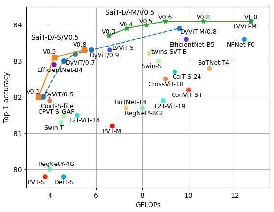
Figure 3: Comparison of SaiT-LV with SOTA models. Green and orange lines represents unified models of SaiT-LV-M and SaiT-LV-S respectively. SaiT-LV is trained end-to-end once and inferred at various token densities (0.3 to 0.8). SaiT-LV outperforms the existing SOTA models with better accuracy-computation(FLOPs) tradeoffs.

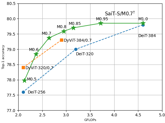
Figure 4: Accuracy-computation (FLOPs) tradeoffs of the SaiT-S/M0.7^† model. Green line represents SaiT-S^† inferred at various mass thresholds on the fly. Orange and blue dash lines connect multiple DyViT and DeiT models with various hidden dimensions. A single SaiT-S^† model offers a range of accuracy-computation results outperforming a series of DeiT models.

Table 1: Comparison of top-1 accuracy between SaiT and some SOTA models.

Models	Params (M)	GFLOPs	Top-1 Acc.
PVT-S (Wang et al., 2021a)	24.5	3.8	79.8
DeiT-S (Touvron et al., 2021a)	22.1	4.6	79.8
CrossViT-S (Chen et al., 2021a)	26.7	5.6	81.0
Swin-T (Liu et al., 2021a)	29	4.5	81.3
T2T-ViT-14 (Yuan et al., 2021)	21.5	5.2	81.5
Twins-SVT-S (Chu et al., 2021)	24	2.8	81.7
CaiT-XS (Touvron et al., 2021b)	26.6	5.4	81.8
CoaT-Lite-S (Xu et al., 2021)	20	4.0	81.9
DeepViT-S (Zhou et al., 2021)	27	6.2	82.3
EfficientNet-B4 (Tan & Le, 2019)	19.3	4.2	82.9
LVViT-S (Jiang et al., 2021)	26.2	6.6	83.3
DyViT-LV-S/0.7 (Rao et al., 2021)	26.9	4.6	83.0
SaiT-LV-S/V0.5	26.2	4.3	83.1
T2T-ViT-24 (Yuan et al., 2021)	64.1	14.1	82.3
CaiT-S (Touvron et al., 2021b)	46.9	9.4	82.7
Swin-S (Liu et al., 2021a)	50	8.7	83.0
Twins-SVT-B (Chu et al., 2021)	56	8.3	83.2
EfficientNet-B5 (Tan & Le, 2019)	30.0	9.9	83.6
NFNet-F0 (Brock et al., 2021)	72	12.4	83.6
LVViT-M (Jiang et al., 2021)	55.8	12.7	84.1
DyViT-LV-M/0.7 (Rao et al., 2021)	57.1	8.5	83.8
SaiT-LV-M/V0.5	55.8	8.2	84.0

In this section, we compare the performances of SaiT with various state-of-the-art (SOTA) vision transformer models, as well as representative CNN models. We explore the accuracy and throughput tradeoffs in the unified model. In addition, we analyze the impact of dense/sparse alternate training and knowledge distillation through an ablation study. The performance impacts of various factors are also discussed, such as sparsification strategies, mass thresholds, and distillation teachers.

4.1 Setup

SaiT-S and SaiT-LV share the same architectural configurations and training schedules as DeiT-S (Touvron et al., 2021a) and LVViT (Jiang et al., 2021), respectively. The implementation is based on the Timm library (Wightman, 2019). ILSVRC-2012 ImageNet (Deng et al., 2009) is used for training and evaluation with the input resolution as 224$\times$224. We train SaiT-S and SaiT-LV from scratch with the proposed training framework for 300 epochs and 410 epochs, respectively. The default batch size is 1024 on 4 GPUs. The default distillation ratio ($\beta$) is 4. For ease of notation, we use SaiT/M0.7 and SaiT/V0.5 to represent the models trained with a mass-based threshold of 0.7 and with a value-based token density of 0.5, respectively. The default pruning location is Layer 3 for SaiT-S and SaiT-LV-S, and Layer 5 for SaiT-LV-M. During training, the default mass threshold and token density are 0.7 and 0.5. For inference, the mass threshold and token density change between 0 to 1 on the fly, subject to the accuracy and throughput requirements. The models with and without distillation are denoted as SaiT^† and SaiT respectively.

4.2 Comparison with SOTA

As shown in Figure 4, SaiT-LV offers the best accuracy for given computation budgets (FLOPs) than other SOTA models. One unified model, SaiT-LV-M/V0.5, offers a range of accuracy 83.7% - 84.1% with 6.6 - 12.6 GFLOPs when inferred at token densities of 0.3 - 1.0. The computation efficiency of SaiT-LV outperforms not only transformer-based architectures but also CNN-based models such as EfficientNet(Tan & Le, 2019), RegNet(Radosavovic et al., 2020), and NFNet(Brock et al., 2021). Specifically, as shown in Table 1, SaiT-LV-S/V0.5 and SaiT-LV-M/V0.5 achieve 1.8% and 1.0% higher accuracy than Swin-T and Swin-S, with 0.2G and 0.5G fewer FLOPs respectively. Moreover, SaiT-LV-S/V0.5 and SaiT-LV-M/V0.5 surpass EfficientNet-B4 and EfficientNet-B5 by 0.2% and 0.4% in top-1 accuracy with the same and 1.8G fewer FLOPs, respectively.

4.3 Accuracy and throughput tradeoff

Table 2: Comparison of throughput improvements between SaiT, DyViT (Rao et al., 2021), and EViT (Liang et al., 2022) over baseline models. Throughput is measured on one 48GB RTX Quadro-8000 GPU with a batch size of 64, following the same procedure in (Liu et al., 2021a). ¹SaiT-S/M0.7^† uses averaged token density and GFLOPs.

Models	Top-1 Acc.	Params (M)	Token Density	GFLOPs	Throughput (im/s)
DeiT-S	79.8	22.1	1.0	4.6	740.7
DyViT-S/0.7	79.3 (-0.5)	22.8 (+0.7)	[0.7/0.49/0.34]	2.9 (-37%)	1155.6 (+56%)
EViT-S	79.5 (-0.3)	22.1 (-)	[0.7/0.49/0.34]	3.0 (-35%)	1146.7 (+55%)
SaiT-S/M0.7†	79.4 (-0.4)	22.1 (-)	0.421	2.6 (-43%)1	1413.6 (+91%)
LVViT-S	83.3	26.2	1.0	6.6	614.0
DyViT-LV-S/0.7	83.0 (-0.3)	26.9 (+0.7)	[0.7/0.49/0.34]	4.6 (-31%)	820.5 (+34%)
SaiT-LV-S/V0.5	82.9 (-0.4)	26.2 (-)	0.42	4.0 (-39%)	1025.1 (+67%)
LVViT-M	84.1	55.8	1.0	12.7	340.5
DyViT-LV-M/0.7	83.8 (-0.3)	57.1 (+1.3)	[0.7/0.49/0.34]	8.5 (-33%)	493.1 (+45%)
SaiT-LV-M/V0.5	83.9 (-0.2)	55.8 (-)	0.4	7.4 (-42%)	581.5 (+71%)

SaiT adopts one-stage pruning with no extra token selection modules, as opposed to three-stage sparsification in DyViT (Rao et al., 2021) (with explicit token selection modules) and EViT (Liang et al., 2022). Additional pruning stages and token selection modules increase the computation, processing time, and memory footprint. As a result, SaiT achieves better accuracy and throughput tradeoff with fewer parameters. Specifically, compared to the baseline DeiT-S and LVViT, SaiT boosts the throughput by 67-91% with around 40% token density and less than 0.5% accuracy loss, as shown in Table 2. This throughput gain is 26-35% higher than DyViT and EViT with similar accuracy.

Furthermore, SaiT-S covers a range of accuracy and throughput when inferred at different mass thresholds. As shown in Figure 4, SaiT-S/M0.7^† outperforms DeiT-256, DeiT-320, DeiT-384, as well as the pruned models DyViT-384/0.7 at various computation complexities (FLOPs). Compared to training and storing a series of different models, SaiT saves training cost and memory footprint with one unified model.

4.4 Weight sharing across various token densities

As shown in Table 3, one SaiT-S/M0.7^† model achieves 0.1% to 0.5% higher accuracy and 7% to 19% higher throughput than a series of EViTs trained separately at various keep rates (token densities). Moreover, training a unified model which is optimized simultaneously for various token sparsities, reduces training cost and memory footprint. Therefore, even with the additional costs from the knowledge distillation, overall SaiT saves training costs by training a single model once as opposed to training a series of models individually.

Table 3: Performance comparison between EViT-S (Liang et al., 2022) and SaiT-S. Density¹ is averaged across the validate set and GFLOPs¹ is obtained based on the averaged density. Throughput is measured on one 48GB RTX Quadro-8000 GPU with a batch size of 64, following the same procedure in (Liu et al., 2021a). Note EViT-S* are five separated models trained individually with keep rates from 0.5 to 0.9.

Keep rate	GFLOPs	Top-1 Acc.	Throughput	$M_{th}$/Density1	GFLOPs1	Top-1 Acc.	Throughput
DeiT	4.6	79.8	740.7	DeiT	4.6	79.8	740.7
EViT-S*				SaiT-S/M0.7†
0.9	4.0 (-13%)	79.8 (-0.0)	858 (+16%)	0.95/0.74	3.7 (-19%)	79.8 (-0.0)	999 (+35%)
0.8	3.5 (-24%)	79.8 (-0.0)	993 (+34%)	0.92/0.68	3.5 (-24%)	79.8 (-0.0)	1060 (+43%)
0.7	3.0 (-35%)	79.5 (-0.3)	1146 (+55%)	0.8/0.52	3.0 (-35%)	79.6 (-0.2)	1264 (+71%)
0.6	2.6 (-43%)	78.9 (-0.9)	1315 (+78%)	0.7/0.42	2.6 (-43%)	79.4 (-0.4)	1414 (+91%)
0.5	2.3 (-50%)	78.5 (-1.3)	1486 (+100%)	0.6/0.34	2.4 (-48%)	78.8 (-1.0)	1543 (107%)

4.5 Ablation study

Dense/sparse alternate training and DINO distillation As shown in Table 4, for SaiT-S/V0.5, the naive approach to train later layers solely with 50% sparse tokens results in 1.0% accuracy loss. Training early layers with a DINO teacher alone improves the model accuracy only with dense tokens, but not for sparse tokens. Subsequently, the most effective approach is to combine dense/sparse alternate training and DINO distillation, improving the accuracy of both dense and sparse tokens simultaneously. The resulting model preserves the baseline accuracy when skipping sparsification and has a 0.4% accuracy loss when processing only 50% of the patch tokens.

Table 4: Impact of dense/sparse alternate training and DINO distillation for SaiT-S/V0.5^†

Pruning	Alternate training	DINO Distillation	Acc. w/100% tokens	Acc. w/ 50% tokens
$\times$	$\times$	$\times$	79.8	77.9 (-1.9)
✓	$\times$	$\times$	78.8 (-1.0)	78.8 (-1.0)
$\times$	$\times$	✓	80.1 (+0.3)	77.8 (-2.0)
✓	$\times$	✓	79.2 (-0.6)	79.2 (-0.6)
✓	✓	$\times$	79.7 (-0.1)	79.2 (-0.6)
✓	✓	✓	79.8 (–)	79.4 (-0.4)

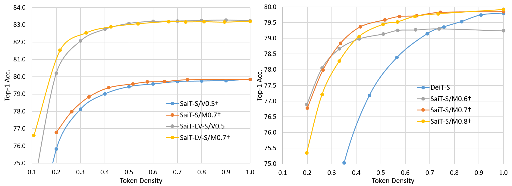
Figure 5: a) Top-1 accuracy for SaiT-S and SaiT-LV-S with mass-based and value-based sparsification strategies inferred at various thresholds and token densities. b) Top-1 accuracy of SaiT-S trained with different mass thresholds (0.6, 0.7, and 0.8), inferred at various thresholds (averaged token densities).

Different sparsification strategies We study the impact of sparsification strategies in Figure 5 a). For both SaiT-S and SaiT-LV-S, mass-based strategy outperforms value-based strategy when token densities is below 0.5. This is attributed to the mass-based adaptive pruning, which adjusts the number of tokens according to the input images. Token densities for mass-based strategy are averaged across all the validation-set images. Note SaiT-LV-S/M0.7^† starts pruning at Layer 4 with more discussion in supplementary materials.

Different mass thresholds We also evaluate the impact of different mass thresholds for training SaiT-S^† (Figure 5 b). Compared to the model with mass threshold of 0.7, training with a smaller threshold of 0.6 leads to inferior inference accuracy at high token densities (0.3 - 1.0), whereas a larger threshold of 0.8 results in more accuracy loss at the low token density regime ($<$0.5) . We hypothesize that a smaller threshold reduce the number of available patch tokens to train later layers, and a large threshold is less effective to train the model with low token density. As a result, the mass threshold is set to be 0.7, for optimal inference accuracy of a wide range of token densities (0.2 - 0.9).

Different distillation teachers To evaluate the impact of distillation teachers, we compare the SaiT-S^† performances with knowledge distillation from pre-trained DeiT-S and DINO. As shown in Table 5, DINO as the teacher outperforms pre-trained DeiT-S for both dense and sparse tokens by 1.6% and 2.3% in top-1 accuracy respectively. This is because DeiT-S tends to allocate some large $TIS$ values to the background patches whereas DINO focuses more effectively on the target object (Caron et al., 2021).

Table 5: Impact of different distillation teachers

Teacher model	Acc. w/100% tokens	Acc. w/50% tokens
DeiT-S	78.2	77.1
DINO	79.8	79.4

5 Conclusion

In this work, we introduce a unified model with a range of accuracy and throughput tradeoffs for different applications. This is achieved through the dense/sparse training framework, knowledge distillation, and parameter-free token sparsification. The adaptive pruning scheme optimizes the token sparsity based on the difficulties of the inputs. SaiT preserves original accuracy when skipping sparsification, and achieves different levels of acceleration by changing token density on the fly. For various vision transformer architectures, the proposed approach effectively reduces 39-43% FLOPs while increasing the throughput by 67-91% with less than 0.5% accuracy drop. Future works can extend the proposed methodologies to transformer/CNN hybrid models and downstream tasks.

Appendix A Appendix

A.1 Token Selection: TIS vs. CLS

We compared the performances of SaiT-S/V0.5 using TIS and CLS for token selection (Table 6) since the CLS token is an alternative to TIS for token selection. However, when training with the CLS selector, the final model results in 0.3% lower accuracy than the model based on TIS when inferred at dense (100%) and sparse (50%) tokens.

Table 6: Impact of different token selection methods: CLS vs. TIS on SaiT-S/V0.5

Token selection	Acc. w/100% tokens	Acc. w/50% tokens
TIS	79.7	79.2
CLS	79.4	78.9

A.2 Distillation ratio

To find the optimal distillation ratio for training, we test the values $\beta\in\{2,4,6\}$ on SaiT-S/V0.5. The resulting top-1 accuracies with dense (100%) tokens and sparse (50%) tokens are listed in Table 7. Different distillation ratios result in no difference for 50% sparse tokens. Using a distillation ratio of 4 leads to 0.1% higher accuracy for 100% dense tokens. Based on SaiT-S/V0.5, top-1 accuracy of both dense and sparse tokens is relatively insensitive to the distillation ratio over this range. As a result, we use $\beta=4$ as the default value in this work.

Table 7: Top-1 accuracy of SaiT-S/V0.5$\dagger$ trained with various distillation ratios

distillation ratio ($\beta$)	Acc. w/100% tokens	Acc. w/50% tokens
2	79.8	79.4
4	79.9	79.4
6	79.8	79.4

A.3 Comparison between EViT and SaiT

Similarly, SaiT-LV-S/V0.5 achieves 0.1% and 0.2% higher accuracy than EViT as shown in Table 8. The throughput improvements over the baseline LVViT model are similar, with SaiT-LV-S slightly higher. Note the throughputs for EViT are from the original paper measured on one A100 machine. We could not find the pretrained EViT-LV-S in time for direct comparison at the same machine.

Same as SaiT-S, one single SaiT-LV-S model achieves competitive accuracy and throughput as two EViT-LV-S models optimized individually at 0.5 and 0.7 keep rates.

Table 8: Performance comparison of EViT-LV-S and SaiT-LV-S. Note EViT-LV-S* are two separated models trained with keep rates at 0.7 and 0.5, whereas SaiT-LV-S/V0.5 is one unified model, trained once with value-based pruning at 0.5 token density and inferred at various token densities. Throughputs of SaiT-LV-S are measured on one 48GB RTX Quadro-8000 GPU with a batch size of 64, following the same procedure in (Liu et al., 2021a). ¹ Throughputs of EViT-LV-S* are from (Liang et al., 2022) measured on one A100 GPU.

Keep rate	GFLOPs	Top-1 Acc.	Throughput	Token density	GFLOPs	Top-1 Acc.	Throughput
LVViT	6.6	83.3	21121	LVViT	6.6	83.3	614
EViT-LV-S*				SaiT-LV-S/V0.5
0.7	4.7 (-29%)	83.0 (-0.3)	2954 (+40%)1	0.5	4.3 (-35%)	83.1 (-0.2)	942 (+53%)
0.5	3.9 (-41%)	82.5 (-0.8)	3603 (+71%)1	0.4	3.9 (-41%)	82.7 (-0.6)	1056 (+72%)

A.4 Token sparsification sensitivity of DeiT-S

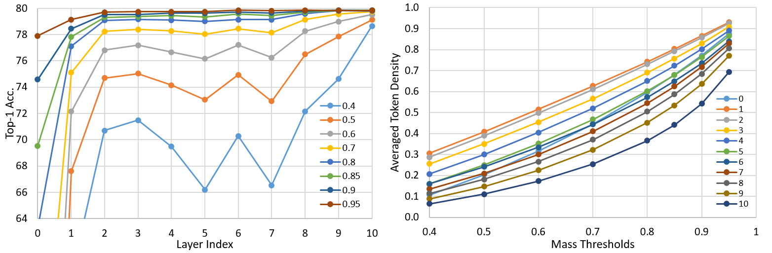
Figure 6: a) Token sparsification sensitivity of DeiT-S: top-1 accuracy when pruned at Layer 0 to Layer 10 with various mass thresholds 0.4 - 0.95. b) Averaged token density with various mass thresholds when pruned at Layer 0 to Layer 10.

Finding the ideal pruning location needs to balance the following two effects. The earlier the pruning starts, the more computation savings are achieved. However, the capacity to learn $TIS$ is constrained if there are too few transformer modules before the pruning location. To address this problem, we analyze the token sparsification sensitivity of DeiT-S as shown in Figure 6.

For the mass-based sparsification scheme, starting at the first two layers leads to significant accuracy drop (Figure 6 a). Layer 3 presents a local optimum, outperforming Layer 2 and Layer 4-5 at various mass thresholds. We hypothesize this results from the $TIS$ distribution along the depth direction as shown in Figure 6 b). With the same mass threshold, the token density decreases monotonically from Layer 1 to Layer 10. Therefore, we choose Layer 3 as the pruning location in SaiT-S, balancing the accuracy drop and computation savings. Similarly, Layer 3 and Layer 5 are chosen as the pruning locations for SaiT-LV-S and SaiT-LV-M, respectively. Token sparsification sensitivity analysis of LVViT is included in the supplemental materials. Empirically, we find that the optimal pruning layer locates at around Layer $L/4$.

A.5 Token sparsification sensitivity of LVViT-S

Mass-based sparsification strategy

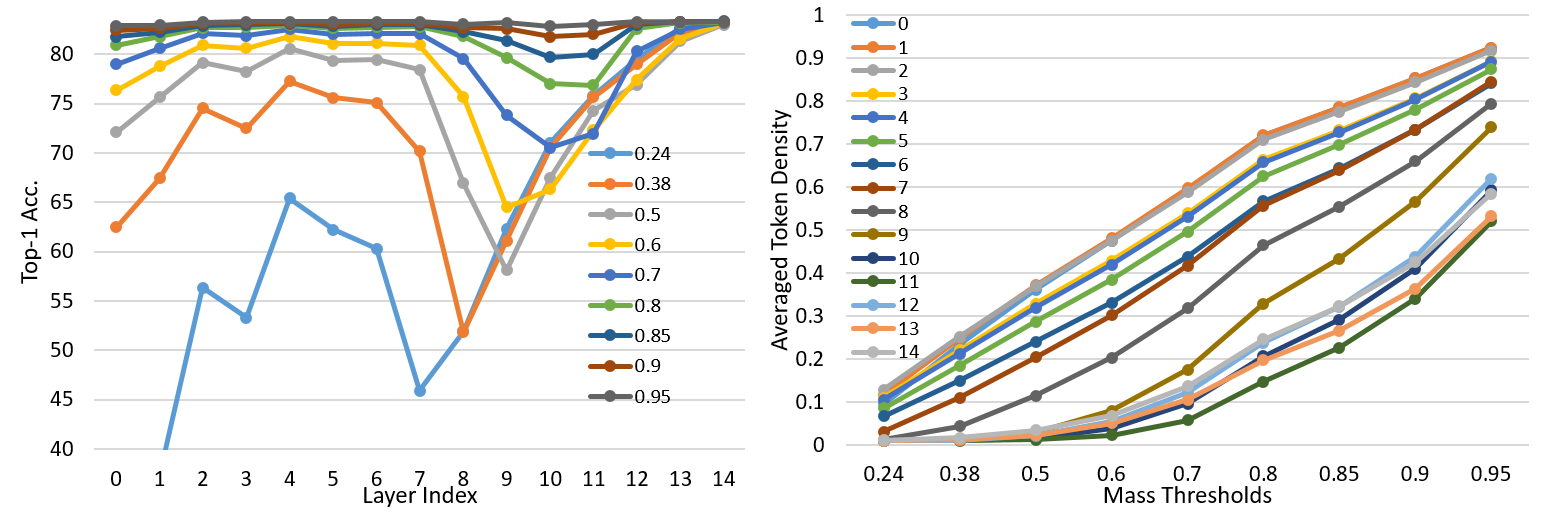
Figure 7: a) Mass-based token sparsification sensitivity of LVViT-S: top-1 accuracy when pruned at Layer 0 to Layer 14 with various mass thresholds ranging from 0.24 to 0.95. b) Averaged token densities with various mass thresholds when pruned at Layer 0 to Layer 14.

As with DeiT-S, the first four layers of LVViT are most sensitive to pruning with significant accuracy drop. As shown in Figure 7 a), Layer 4 is a local optimum for various mass thresholds. Therefore, we choose Layer 4 as the token pruning location for the mass-based sparsification scheme.

However, unlike DeiT-S, under the same mass threshold, the token density of LVViT-S no longer decreases monotonically from Layer 1 to Layer 14 (Figure 7 b). Instead, Layer 10 and Layer 11 show lower average token density than Layer 13 and Layer 14 under the same mass threshold. We hypothesize this results from the auxiliary dense patch token labels used by LVViT. Besides learning from the classification label with the classification token, LVViT also leverages the feature representation from all the patch tokens and learns from the patch labels. Therefore, the probability mass at the last few layers is re-distributed across all the patch tokens, as opposed to being more concentrated in the $CLS$ token as in DeiT.

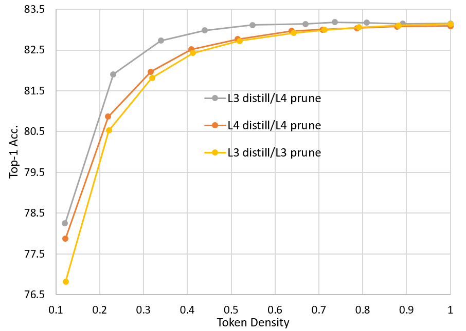
Figure 8: Top-1 accuracy of SaiT-LV-S/M0.7 trained with different knowledge distillation locations and pruning locations. L3 distill/L4 prune denotes the knowledge distillation at Layer 3 and pruning location at Layer 4, while L3 distill/L3 prune represents both knowledge distillation and pruning location at Layer 4, and the same applies to L4 distill/L4 prune.

Using auxiliary labels for all patch tokens also presents unique challenges for knowledge distillation with LVViT, since the classification token from the last layer only contains partial information regarding token importance. To address this issue, we find that performing distillation at Layer 3 and pruning at Layer 4 yields the best performances as shown in Figure 8. Changing the distillation and pruning location from Layer 3 to Layer 4 only slightly improves the accuracy for averaged token density below 40%. On the other hand, moving the knowledge distillation location to Layer 3 and keeping the pruning location at Layer 4 significantly improves the accuracy for a wide range of token densities between 0.1 and 0.8. We hypothesize this change injects knowledge from the classification token of the last layer while also allowing more pruning flexibility at Layer 4, which leads to higher accuracy.

Value-based sparsification strategy

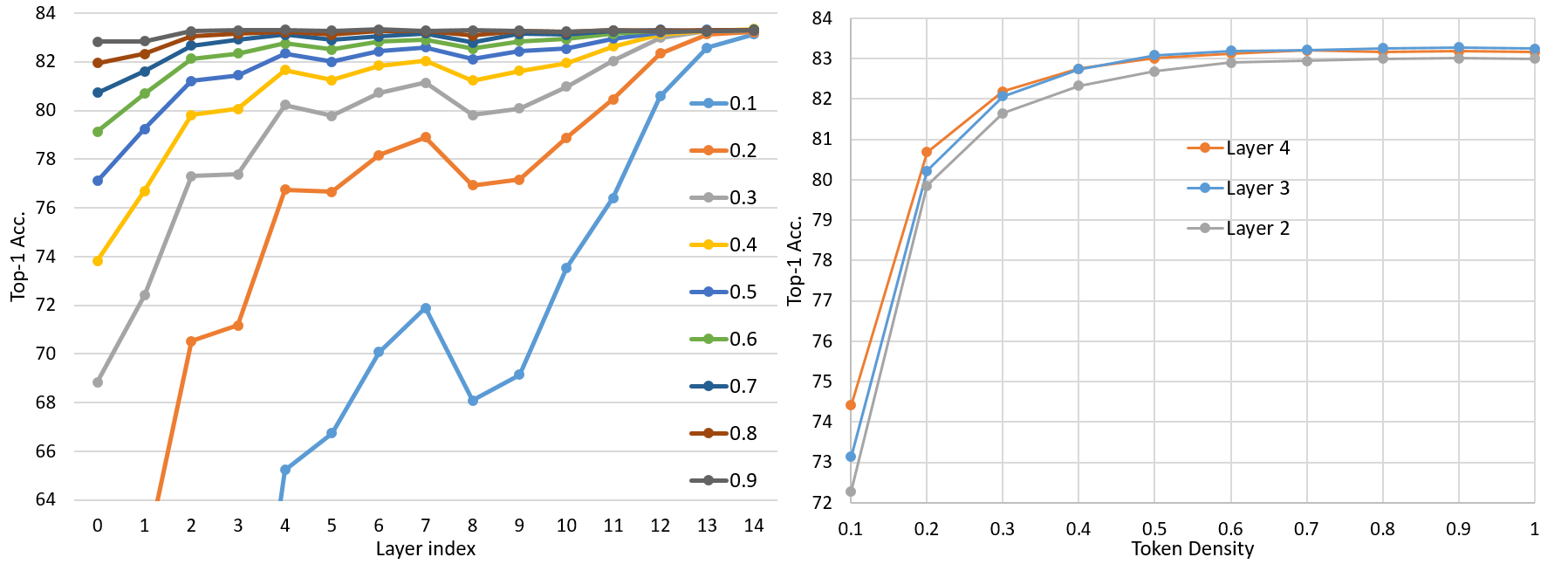
Figure 9: a) Value-based token sparsification sensitivity for LVViT-S: top-1 accuracy when pruned at Layer 0 to Layer 14 with various token densities 0.1 to 1.0 during inference. b) Top-1 accuracy of SaiT-LV-S/V0.5 when training with pruning location at Layer 2, Layer 3, and Layer 4 respectively.

Similarly, for value-based sparsification (Figure 9 a), Layer 4 is a local optimum for token densities between 0.2 and 0.7. The differences across different layers get smaller with increasing token densities. Layer 8 and Layer 9 present an accuracy dip, compared to Layer 7 and Layer 10. We hypothesize that different token probability distributions across Layer 8 to Layer 14 are the main cause of the accuracy dip. As a result, we choose not to use knowledge distillation for value-based SaiT-LV models.

As shown in Figure 9 b), there is little difference in top-1 accuracy of SaiT-LV-S/V0.5 trained with Layer 3 and Layer 4 as the pruning location. However, when moving the pruning location to Layer 2, SaiT-LV-S/V0.5 suffers an average accuracy loss of around 0.3-0.4% for various token densities. Therefore, to maximize computation savings while maintaining accuracy, we choose Layer 3 as the default pruning location for SaiT-LV-S/V0.5.

A.6 Number of training epochs

We compare the performances of SaiT-LV-S/V0.5 and SaiT-LV-M/V0.5 trained for 310 and 410 epochs as shown in Figure 10. With more parameters and model capacity, the extra 100 epochs of training barely change the accuracy of SaiT-LV-M/V0.5. On the other hand, for SaiT-LV-S/V0.5, 100 more epochs increase the top-1 accuracy by 0.3% to 0.5% when inferred at various token densities (0.2 -1.0). As a result, we choose to train the SaiT-LV for 410 epochs to achieve better inference accuracy.

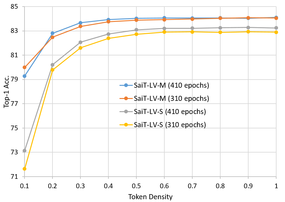
Figure 10: Top-1 accuracy of SaiT-LV-S/V0.5 and SaiT-LV-M/V0.5 trained for 310 epochs and 410 epochs.

References

- Brock et al. (2021) Andrew Brock, Soham De, Samuel L. Smith, and Karen Simonyan. High-performance large-scale image recognition without normalization, 2021.
- Carion et al. (2020) Nicolas Carion, Francisco Massa, Gabriel Synnaeve, Nicolas Usunier, Alexander Kirillov, and Sergey Zagoruyko. End-to-end object detection with transformers, 2020.
- Caron et al. (2021) Mathilde Caron, Hugo Touvron, Ishan Misra, Hervé Jégou, Julien Mairal, Piotr Bojanowski, and Armand Joulin. Emerging properties in self-supervised vision transformers. In Proceedings of the International Conference on Computer Vision (ICCV), 2021.
- Chen et al. (2021a) Chun-Fu Chen, Quanfu Fan, and Rameswar Panda. Crossvit: Cross-attention multi-scale vision transformer for image classification, 2021a.
- Chen et al. (2021b) Tianlong Chen, Yu Cheng, Zhe Gan, Lu Yuan, Lei Zhang, and Zhangyang Wang. Chasing sparsity in vision transformers: An end-to-end exploration. In M. Ranzato, A. Beygelzimer, Y. Dauphin, P.S. Liang, and J. Wortman Vaughan (eds.), Advances in Neural Information Processing Systems, volume 34, pp. 19974–19988. Curran Associates, Inc., 2021b.
- Cheng et al. (2021) Bowen Cheng, Alexander G. Schwing, and Alexander Kirillov. Per-pixel classification is not all you need for semantic segmentation, 2021.
- Chu et al. (2021) Xiangxiang Chu, Zhi Tian, Yuqing Wang, Bo Zhang, Haibing Ren, Xiaolin Wei, Huaxia Xia, and Chunhua Shen. Twins: Revisiting the design of spatial attention in vision transformers, 2021.
- Deng et al. (2009) Jia Deng, Wei Dong, Richard Socher, Li-Jia Li, Kai Li, and Li Fei-Fei. Imagenet: A large-scale hierarchical image database. In CVPR, pp. 248–255. Ieee, 2009.
- Dosovitskiy et al. (2021) Alexey Dosovitskiy, Lucas Beyer, Alexander Kolesnikov, Dirk Weissenborn, Xiaohua Zhai, Thomas Unterthiner, Mostafa Dehghani, Matthias Minderer, Georg Heigold, Sylvain Gelly, et al. An image is worth 16x16 words: Transformers for image recognition at scale. In ICLR, 2021.
- Gong et al. (2014) Yunchao Gong, Liu Liu, Ming Yang, and Lubomir Bourdev. Compressing deep convolutional networks using vector quantization, 2014.
- Graham et al. (2021) Ben Graham, Alaaeldin El-Nouby, Hugo Touvron, Pierre Stock, Armand Joulin, Hervé Jégou, and Matthijs Douze. Levit: a vision transformer in convnet’s clothing for faster inference, 2021.
- Guo et al. (2021) Jianyuan Guo, Kai Han, Han Wu, Chang Xu, Yehui Tang, Chunjing Xu, and Yunhe Wang. Cmt: Convolutional neural networks meet vision transformers, 2021.
- Han et al. (2015) Song Han, Huizi Mao, and William J. Dally. Deep compression: Compressing deep neural networks with pruning, trained quantization and huffman coding, 2015.
- He et al. (2016) Kaiming He, Xiangyu Zhang, Shaoqing Ren, and Jian Sun. Deep residual learning for image recognition. In CVPR, pp. 770–778, 2016.
- He et al. (2021) Kaiming He, Xinlei Chen, Saining Xie, Yanghao Li, Piotr Dollár, and Ross Girshick. Masked autoencoders are scalable vision learners, 2021.
- Hinton et al. (2015) Geoffrey Hinton, Oriol Vinyals, and Jeff Dean. Distilling the knowledge in a neural network, 2015.
- Jaegle et al. (2021) Andrew Jaegle, Felix Gimeno, Andrew Brock, Andrew Zisserman, Oriol Vinyals, and Joao Carreira. Perceiver: General perception with iterative attention, 2021.
- Jiang et al. (2021) Zihang Jiang, Qibin Hou, Li Yuan, Daquan Zhou, Yujun Shi, Xiaojie Jin, Anran Wang, and Jiashi Feng. All tokens matter: Token labeling for training better vision transformers. arXiv preprint arXiv:2104.10858, 2021.
- Krizhevsky et al. (2012) Alex Krizhevsky, Ilya Sutskever, and Geoffrey E Hinton. Imagenet classification with deep convolutional neural networks. NIPS, 25:1097–1105, 2012.
- Li et al. (2021a) Changlin Li, Tao Tang, Guangrun Wang, Jiefeng Peng, Bing Wang, Xiaodan Liang, and Xiaojun Chang. Bossnas: Exploring hybrid cnn-transformers with block-wisely self-supervised neural architecture search, 2021a.
- Li et al. (2022) Yanghao Li, Hanzi Mao, Ross Girshick, and Kaiming He. Exploring plain vision transformer backbones for object detection, 2022.
- Li et al. (2021b) Yawei Li, Kai Zhang, Jiezhang Cao, Radu Timofte, and Luc Van Gool. Localvit: Bringing locality to vision transformers, 2021b.
- Liang et al. (2022) Youwei Liang, Chongjian GE, Zhan Tong, Yibing Song, Jue Wang, and Pengtao Xie. EVit: Expediting vision transformers via token reorganizations. In International Conference on Learning Representations, 2022.
- Liu et al. (2021a) Ze Liu, Yutong Lin, Yue Cao, Han Hu, Yixuan Wei, Zheng Zhang, Stephen Lin, and Baining Guo. Swin transformer: Hierarchical vision transformer using shifted windows, 2021a.
- Liu et al. (2021b) Zhenhua Liu, Yunhe Wang, Kai Han, Wei Zhang, Siwei Ma, and Wen Gao. Post-training quantization for vision transformer. In A. Beygelzimer, Y. Dauphin, P. Liang, and J. Wortman Vaughan (eds.), Advances in Neural Information Processing Systems, 2021b.
- Radosavovic et al. (2020) Ilija Radosavovic, Raj Prateek Kosaraju, Ross Girshick, Kaiming He, and Piotr Dollár. Designing network design spaces. In CVPR, pp. 10428–10436, 2020.
- Rao et al. (2021) Yongming Rao, Wenliang Zhao, Benlin Liu, Jiwen Lu, Jie Zhou, and Cho-Jui Hsieh. Dynamicvit: Efficient vision transformers with dynamic token sparsification. In Advances in Neural Information Processing Systems (NeurIPS), 2021.
- Srinivas et al. (2021) Aravind Srinivas, Tsung-Yi Lin, Niki Parmar, Jonathon Shlens, Pieter Abbeel, and Ashish Vaswani. Bottleneck transformers for visual recognition, 2021.
- Sun et al. (2017) Chen Sun, Abhinav Shrivastava, Saurabh Singh, and Abhinav Gupta. Revisiting unreasonable effectiveness of data in deep learning era, 2017.
- Tan & Le (2019) Mingxing Tan and Quoc Le. Efficientnet: Rethinking model scaling for convolutional neural networks. In ICML, pp. 6105–6114. PMLR, 2019.
- Touvron et al. (2021a) Hugo Touvron, Matthieu Cord, Matthijs Douze, Francisco Massa, Alexandre Sablayrolles, and Herve Jegou. Training data-efficient image transformers & distillation through attention. In ICML, volume 139, pp. 10347–10357, July 2021a.
- Touvron et al. (2021b) Hugo Touvron, Matthieu Cord, Alexandre Sablayrolles, Gabriel Synnaeve, and Hervé Jégou. Going deeper with image transformers. arXiv preprint arXiv:2103.17239, 2021b.
- Wang et al. (2021a) Wenhai Wang, Enze Xie, Xiang Li, Deng-Ping Fan, Kaitao Song, Ding Liang, Tong Lu, Ping Luo, and Ling Shao. Pyramid vision transformer: A versatile backbone for dense prediction without convolutions, 2021a.
- Wang et al. (2021b) Yulin Wang, Rui Huang, Shiji Song, Zeyi Huang, and Gao Huang. Not all images are worth 16x16 words: Dynamic vision transformers with adaptive sequence length, 2021b.
- Wightman (2019) Ross Wightman. Pytorch image models. https://github.com/rwightman/pytorch-image-models, 2019.
- Wu et al. (2021a) Haiping Wu, Bin Xiao, Noel Codella, Mengchen Liu, Xiyang Dai, Lu Yuan, and Lei Zhang. Cvt: Introducing convolutions to vision transformers, 2021a.
- Wu et al. (2021b) Lemeng Wu, Xingchao Liu, and Qiang Liu. Centroid transformers: Learning to abstract with attention, 2021b.
- Xu et al. (2021) Weijian Xu, Yifan Xu, Tyler Chang, and Zhuowen Tu. Co-scale conv-attentional image transformers, 2021.
- Yuan et al. (2021) Li Yuan, Yunpeng Chen, Tao Wang, Weihao Yu, Yujun Shi, Zihang Jiang, Francis EH Tay, Jiashi Feng, and Shuicheng Yan. Tokens-to-token vit: Training vision transformers from scratch on imagenet, 2021.
- Zheng et al. (2021) Sixiao Zheng, Jiachen Lu, Hengshuang Zhao, Xiatian Zhu, Zekun Luo, Yabiao Wang, Yanwei Fu, Jianfeng Feng, Tao Xiang, Philip H.S. Torr, and Li Zhang. Rethinking semantic segmentation from a sequence-to-sequence perspective with transformers. In CVPR, 2021.
- Zhou et al. (2021) Daquan Zhou, Bingyi Kang, Xiaojie Jin, Linjie Yang, Xiaochen Lian, Zihang Jiang, Qibin Hou, and Jiashi Feng. Deepvit: Towards deeper vision transformer, 2021.