Cramér–Rao Lower Bound Optimization for Hidden Moving Target Sensing via Multi-IRS-Aided Radar

Abstract

Intelligent reflecting surface (IRS) is a rapidly emerging paradigm to enable non-line-of-sight (NLoS) wireless transmission. In this paper, we focus on IRS-aided radar estimation performance of a moving hidden or NLoS target. Unlike prior works that employ a single IRS, we investigate this problem using multiple IRS platforms and assess the estimation performance by deriving the associated Cramér-Rao lower bound (CRLB). We then design Doppler-aware IRS phase shifts by minimizing the scalar A-optimality measure of the joint parameter CRLB matrix. The resulting optimization problem is non-convex, and is thus tackled via an alternating optimization framework. Numerical results demonstrate that the deployment of multiple IRS platforms with our proposed optimized phase shifts leads to a higher estimation accuracy compared to non-IRS and single-IRS alternatives.

I Introduction

In recent years, intelligent reflecting surfaces (IRS) have emerged as a promising technology for smart wireless environments [1, 2]. An IRS consists of low-cost passive meta-material elements capable of varying the phase of the impinging signal and hence shaping the radiation beampattern to alter the radio propagation environment. Initial research on IRS was limited to wireless communication applications such as range extension to users with obstructed direct links [3], joint wireless information and power transmission [4], physical layer security [5], unmanned air vehicle (UAV) communications [6], and shaping the wireless channel through multi-beam design [7]. Recent works have also introduced IRS to integrated communications and sensing systems [8, 9, 5, 10]. In this paper, we focus on IRS-aided sensing, following the advances made in [11, 8].

The literature on IRS-aided radar [12, 9] is primarily focused on the radar’s ability to sense objects that are hidden from its line-of-sight (LoS). While there is a rich body of research on non-IRS-based non-line-of-sight (NLoS) radars (see, e.g., [13] and the references therein), the proposed formulations require prior and rather accurate knowledge of the geometry of propagation environment. In contrast, IRS-aided radar utilizes the signals received from the NLoS paths to compensate for the end-to-end transmitter-receiver or LoS path loss [11].

The potential of IRS in enhancing the estimation performance of radar systems has been recently investigated in [14, 8, 15]. Some recent studies such as [14], employ IRS to correctly estimate the direction-of-arrival (DoA) of a stationary target. Nearly all of the aforementioned works consider a single-IRS aiding the radar for estimating the parameters of a stationary target. The IRS-based radar-communications in [15] included moving targets but did not examine parameter estimation. In this paper, we focus on the estimation performance of a multi-IRS-aided radar dealing with moving targets.

In particular, we jointly estimate target reflectivity and Doppler velocity with multiple IRS platforms in contrast to the scalar parameter estimation via a single IRS in [14]. We derive the Cramér-Rao lower bound (CRLB) for these parameter estimates and then determine the optimal IRS phase shifts using CRLB as a benchmark. Previously, maximization of signal-to-noise ratio (SNR) or signal-to-interference-to-noise ratio (SINR) was employed in [16] to determine the optimal phase shifts for target detection. However, optimization of the SNR or SINR does not guarantee an improvement in target estimation accuracy. Our previous works [11] and [17] introduced multi-IRS-aided radar for NLoS sensing of a stationary target and derived the best linear unbiased estimator (BLUE) focusing only on target reflectivity and the CRLB of DoA, respectively.

The rest of the paper is organized as follows. In the next section, we introduce the signal model for the multi-IRS-aided radar. In section III, we derive the CRLB for joint parameter estimation. section IV presents the algorithm to optimize the IRS phase shifts. We evaluate our methods via numerical experiments in section V and conclude the paper in section VI.

Throughout this paper, we use bold lowercase and bold uppercase letters for vectors and matrices, respectively. $\mathbb{C}$ and $\mathbb{R}$ represent the set of complex and real numbers, respectively. $(\cdot)^{\top}$ and $(\cdot)^{\mathrm{H}}$ denote the vector/matrix transpose, and the Hermitian transpose, respectively. The trace of a matrix is denoted by $\operatorname{Tr}(.)$. $\textrm{Diag}(.)$ denotes the diagonalization operator that produces a diagonal matrix with same diagonal entries as the entries of its vector argument, while $\textrm{diag}(.)$ outputs a vector containing the diagonal entries of the input matrix. The $mn$-th element of the matrix $\mathbf{B}$ is $\left[\mathbf{B}\right]_{mn}$. The Hadamard (element-wise) and Kronecker products are denoted by notations $\odot$ and $\otimes$, respectively. The element-wise matrix derivation operator is $[\frac{\partial\mathbf{A}}{\partial b}]_{ij}=\frac{\partial\mathbf{A}_{ij}}{\partial b}$. The $s$-dimensional all-one vector and the identity matrix of size $s\times s$ are denoted as $\mathbf{1}_{s}$ and $\mathbf{I}_{s}$, respectively. Finally, $\operatorname{Re}\left(\cdot\right)$ and $\operatorname{Im}\left(\cdot\right)$ return the the real part, and the imaginary part of a complex input vector, respectively.

II System Model

Consider a single-antenna pulse-Doppler IRS-aided radar, which transmits a train of $N$ uniformly-spaced pulses $s(t)$, each of which is nonzero over the support $[0,\tau]$, with the pulse repetition interval (PRI) $T_{{}_{p}}$; its reciprocal $1/T_{{}_{p}}$ is the pulse repetition frequency (PRF). The transmit signal is

$$x(t)=\sum_{n=0}^{N-1}s(t-nT_{{}_{p}}),\;0\leq t\leq(N-1)T_{{}_{p}}.$$ (1)

The entire duration of all $N$ pulses is the coherent processing interval (CPI) following a slow-time coding procedure [19].

Assume that the propagation environment has $K$ IRS platforms, each with $M$ reflecting elements, deployed on stationary platforms at known locations (Fig. 1). Each of the $M$ reflecting elements in the $k$-th IRS or IRS_k reflects the incident signal with a phase shift and amplitude change that is configured via a smart controller [20]. Denote the phase shift matrix of IRS_k by

$$\boldsymbol{\Phi}_{k}=\text{{Diag}}\left(\beta_{k,1}e^{\textrm{j}\phi_{k,1}},\ldots,\beta_{k,M}e^{\textrm{j}\phi_{k,M}}\right),$$ (2)

where $\phi_{k,m}\in[0,2\pi]$, and $\beta_{k,m}\in[0,1]$ are, respectively, the phase shift and the amplitude reflection gain associated with the $m$-th passive element of IRS_k. In practical settings, it usually suffices to design only the phase shifts so that $\beta_{k,m}=1$ for all $(k,m)$. The radar-IRS_k-target-IRS_k-radar channel coefficient/gain is

$$h_{{}_{{\textrm{NLoS}},k}}=\mathbf{b}^{\top}(\theta_{ir,k})\boldsymbol{\Phi}_{k}\mathbf{b}(\theta_{ti,k})\mathbf{b}^{\top}(\theta_{ti,k})\boldsymbol{\Phi}_{k}\mathbf{b}(\theta_{ir,k}),$$ (3)

where $\theta_{ir,k}$ ($\theta_{ti,k}$) is the angle between the radar (target) and IRS_k, and each IRS is a uniform linear array with the inter-element spacing $d$, with the steering vector

$$\mathbf{b}(\theta) =\left[1,e^{\mathrm{j}\frac{2\pi d}{\lambda}\sin\theta},\ldots,e^{\mathrm{j}\frac{2\pi d}{\lambda}(M-1)\sin\theta}\right]^{\top},$$ (4)

and $\lambda$ denoting the carrier wavelength.

Consider a single Swerling-0 model [21], moving target with $f_{{}_{D_{0}}}$ and $\alpha_{0}$ being, respectively, its Doppler frequency and target back-scattering coefficient as observed via the LoS path between the target and radar. Denote the same parameters by, respectively, $f_{{}_{D_{k}}}$ and $\alpha_{{}_{k}}$, for $k\in\left\{1,\ldots,K\right\}$ as observed by the radar from the NLoS path via IRS_k. All Doppler frequencies lie in the unambiguous frequency region, i.e., up to PRF. The received signal in a known range-bin is a superposition of echoes from the LoS and NLoS paths as

$$y(t) =\alpha_{0}h_{{}_{{\textrm{LoS}}}}\sum_{n=0}^{N-1}s(t-nT_{{}_{p}})e^{\mathrm{j}2\pi f_{D_{0}}t}$$

$$+\sum_{k=1}^{K}\sum_{n=0}^{N-1}\alpha_{k}h_{{}_{{\textrm{NLoS}},k}}s(t-nT_{{}_{p}})e^{\mathrm{j}2\pi f_{{}_{D_{k}}}t}+w(t)$$

$$\approx\alpha_{0}h_{{}_{{\textrm{LoS}}}}\sum_{n=0}^{N-1}s(t-nT_{{}_{p}})e^{\mathrm{j}2\pi f_{{}_{D_{0}}}nT_{p}}$$

$$+\sum_{k=1}^{K}\sum_{n=0}^{N-1}\alpha_{k}h_{{}_{{\textrm{NLoS}},k}}s(t-nT_{{}_{p}})e^{\mathrm{j}2\pi f_{{}_{D_{k}}}nT_{p}}+w(t)$$ (5)

where $h_{{}_{{\textrm{LoS}}}}$ is the radar-target-radar LoS channel state information (CSI), $h_{{}_{{\textrm{NLoS}},k}}$ is the NLoS channel through radar-IRS_k-target-IRS_k-radar path, $w(t)$ is the random additive signal-independent interference, and the last approximation assumes the target is moving with low speed $f_{{}_{D_{k}}}\ll 1/\tau$ for $k\in\left\{0,\ldots,K\right\}$ and have low acceleration, so that the phase rotation within the CPI could be approximated as a constant.

We design a radar system to sense a moving target in the two-dimensional (2-D) Cartesian plane. Our proposed signal model and methods are readily extendable to 3-D scenarios by replacing the 1-D DoA with 2-D DoA in  (3) and (4). In particular, we consider a target tracking scenario where the radar wishes to examine a range-cell for a potential target [22, 23]. Accordingly, we collect $N$ slow-time samples of (II) corresponding to $N$ pulses in the vector

$$\mathbf{y}=\alpha_{0}h_{{}_{{\textrm{LoS}}}}\left(\mathbf{x}\odot\mathbf{p}(\nu_{0})\right)+\sum_{k=1}^{K}\alpha_{{}_{k}}h_{{}_{{\textrm{NLoS}},k}}\left(\mathbf{x}\odot\mathbf{p}(\nu_{k})\right)+\mathbf{w},$$ (6)

where $\nu_{k}=2\pi f_{{}_{D_{k}}}T_{p}\in[-0.5,0.5)$ for $k\in\{0,\ldots,K\}$ are the normalized Doppler shifts, $\mathbf{p}(\nu)=\left[1,e^{\mathrm{j}\nu},\ldots,e^{\mathrm{j}(N-1)\nu}\right]^{\top}$ is a generic Doppler steering vector, and $\mathbf{x}=[x(0),x(T_{{}_{p}}),\ldots,x((N-1)T_{{}_{p}})]^{\top}$ and $\mathbf{w}=[w(0),w(T_{{}_{p}}),\ldots,w((N-1)T_{{}_{p}})]^{\top}$ are the $N$-dimensional column vectors of the transmit signal and the zero-mean random noise vector with a covariance $\mathbf{R}$, respectively [24].

Assume the complex target back-scattering coefficients observed from the LoS and NLoS paths are collected in the vector $\boldsymbol{\alpha}=[\alpha_{{}_{0}},\alpha_{{}_{1}},\alpha_{{}_{2}},\ldots,\alpha_{{}_{K}}]^{\top}$. The corresponding channel coefficients are collected in $\mathbf{h}=[h_{{}_{{\textrm{LoS}}}},h_{{}_{{\textrm{NLoS}},1}},\ldots,h_{{}_{{\textrm{NLoS}},K}}]^{\top}$. Denote the sensing matrix by $\mathbf{A}=\left[\mathbf{a}_{0},\mathbf{a}_{1},\ldots,\mathbf{a}_{K}\right]\in\mathbb{C}^{N\times K+1}$, where $\mathbf{a}_{0}=h_{{}_{{\textrm{LoS}}}}\left[\mathbf{x}\odot\mathbf{p}(\nu_{0})\right]$ and $\mathbf{a}_{k}=h_{{}_{{\textrm{NLoS}},k}}\left[\mathbf{x}\odot\mathbf{p}(\nu_{k})\right]$. This implies that $\mathbf{A}=\mathbf{x}\mathbf{h}^{\top}\odot\mathbf{P}(\nu)$, where the Doppler shift matrix is $\mathbf{P}(\boldsymbol{\nu})=[\mathbf{p}(\nu_{0}),\mathbf{p}(\nu_{1}),\ldots,\mathbf{p}(\nu_{K})]\in\mathbb{C}^{N\times K+1}$. Then, the received signal (6) in the vector form is given as

$$\mathbf{y}=\mathbf{A}\boldsymbol{\alpha}+\mathbf{w},$$ (7)

In presence of multiple-IRS platforms (Fig.1), we define the LoS-to-NLoS link strength ratio (LSR) as $\gamma=\frac{|\alpha_{{}_{0}}h_{{}_{{\textrm{LoS}}}}|^{2}}{\sum_{k=1}^{K}|\alpha_{k}h_{{}_{{\textrm{NLoS}},k}}|^{2}}$, which governs the relative strengths of the signals received from both paths. In cases where the LoS path is obstructed or weaker than the NLoS paths as illustrated in Fig. 1, we have $h_{{}_{{\textrm{LoS}}}}\ll h_{{}_{{\textrm{NLoS}},k}}$.

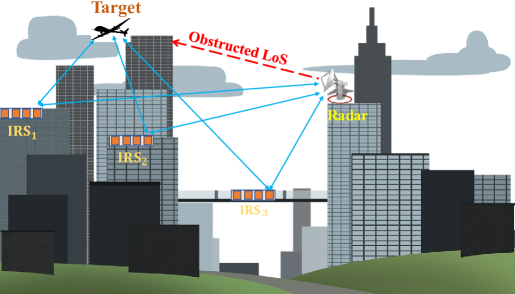
Figure 1: A simplified illustration of various NLoS or virtual LoS links between the radar and the hidden, moving target, provided by multiple IRS platforms mounted on urban infrastructure.

III CRLB for Multi-IRS-Aided Radar

Denote the $3(K+1)\times 1$ vector of unknown target parameters as $\boldsymbol{\zeta}=\left[\tilde{\boldsymbol{\alpha}}^{\top},\boldsymbol{\nu}^{\top}\right]^{\top}$, where $\tilde{\boldsymbol{\alpha}}=[\boldsymbol{\alpha}_{R}^{\top},\boldsymbol{\alpha}_{I}^{\top}]^{\top}$, with $\boldsymbol{\alpha}_{R}=\operatorname{Re}\left(\boldsymbol{\alpha}\right)$, $\boldsymbol{\alpha}_{I}=\operatorname{Im}\left(\boldsymbol{\alpha}\right)$, and $\boldsymbol{\nu}=[\nu_{0},\nu_{1},\ldots,\nu_{K}]^{\top}$ denoting the Doppler shifts vector. For an unbiased estimator $\hat{\boldsymbol{\zeta}}$, the covariance matrix is lower bounded as $\boldsymbol{C}_{\hat{\boldsymbol{\zeta}}}=\mathbf{E}\{{(\hat{\boldsymbol{\zeta}}-\boldsymbol{\zeta})(\hat{\boldsymbol{\zeta}}-\boldsymbol{\zeta})^{H}}\}\geq\boldsymbol{C}_{{}_{\textrm{CRLB}}}$, in the sense that the difference $\boldsymbol{C}_{\hat{\boldsymbol{\zeta}}}-\boldsymbol{C}_{{}_{\textrm{CRB}}}$ is a positive semidefinite matrix. Express the $3(K+1)\times 3(K+1)$ Fisher information matrix (FIM) in terms of the parameter submatrices as

$$\mathbf{F}=\begin{bmatrix}\mathbf{F}_{\tilde{\boldsymbol{\alpha}},\tilde{\boldsymbol{\alpha}}}&\mathbf{F}_{\tilde{\boldsymbol{\alpha}},\boldsymbol{\nu}}\\ \mathbf{F}_{\boldsymbol{\nu},\tilde{\boldsymbol{\alpha}}}&\mathbf{F}_{\boldsymbol{\nu},\boldsymbol{\nu}}\end{bmatrix}=\begin{bmatrix}\boldsymbol{C}_{\tilde{\boldsymbol{\alpha}},\tilde{\boldsymbol{\alpha}}}&\boldsymbol{C}_{\tilde{\boldsymbol{\alpha}},\boldsymbol{\nu}}\\ \boldsymbol{C}_{\boldsymbol{\nu},\tilde{\boldsymbol{\alpha}}}&\boldsymbol{C}_{\boldsymbol{\nu},\boldsymbol{\nu}}\end{bmatrix}^{-1}=\boldsymbol{C}_{{}_{\textrm{CRLB}}}^{-1},$$ (8)

The following Theorem 1 derives each submatrix term.

Theorem 1.

For the signal model in (7), where $\mathbf{w}\sim\mathcal{CN}\left(\boldsymbol{0},\mathbf{R}\right)$, the submatrices of the FIM in (8) are

$$\mathbf{F}_{\tilde{\boldsymbol{\alpha}},\tilde{\boldsymbol{\alpha}}}=2\operatorname{Re}\left(\left[1\;\mathrm{j}\right]^{\mathrm{H}}\otimes\left[1\;\mathrm{j}\right]\otimes\left(\mathbf{A}^{\mathrm{H}}\mathbf{R}^{-1}\mathbf{A}\right)\right),\;\in\mathbb{R}^{2K\times 2K},$$ (9)

$$\mathbf{F}_{\tilde{\boldsymbol{\alpha}},\boldsymbol{\nu}}=\mathbf{F}^{\top}_{\boldsymbol{\nu},\tilde{\boldsymbol{\alpha}}}$$

$$=2\operatorname{Re}\left(\left(\left[1\;\mathrm{j}\right]^{\mathrm{H}}\otimes\left(\mathbf{A}^{\mathrm{H}}\mathbf{R}^{-1}\dot{\mathbf{A}}\right)\right)\left(\boldsymbol{\alpha}\otimes\mathbf{I}_{K}\right)\right),\;\in\mathbb{R}^{2K\times K},$$ (10)

$$\mathbf{F}_{\boldsymbol{\nu},\boldsymbol{\nu}}=2\operatorname{Re}\left(\left(\boldsymbol{\alpha}\otimes\mathbf{I}_{K}\right)^{\mathrm{H}}\left(\dot{\mathbf{A}}^{\mathrm{H}}\mathbf{R}^{-1}\dot{\mathbf{A}}\right)\left(\boldsymbol{\alpha}\otimes\mathbf{I}_{K}\right)\right)\;\in\mathbb{R}^{K\times K}.$$ (11)

Proof:

Using the Slepian-Bangs formula [25; 26, p. 360; 27, p. 565], for the complex observation vector $\mathbf{y}\sim\mathcal{CN}\left(\boldsymbol{\mu},\mathbf{R}\right)$, the $(m,n)$-th element of the FIM $\mathbf{F}$ is

$$[\mathbf{F}]_{mn}=\operatorname{Tr}\left(\mathbf{R}^{-1}\frac{\partial\mathbf{R}}{\partial\boldsymbol{\zeta}_{m}}\mathbf{R}^{-1}\frac{\partial\mathbf{R}}{\partial\boldsymbol{\zeta}_{n}}\right)+2\operatorname{Re}\left(\frac{\partial\boldsymbol{\mu}}{\partial\boldsymbol{\zeta}_{m}}^{H}\mathbf{R}^{-1}\frac{\partial\boldsymbol{\mu}}{\partial\boldsymbol{\zeta}_{n}}\right).$$ (12)

From (7), we have $\boldsymbol{\mu}=\mathbf{A}\boldsymbol{\alpha}$ [27]. Define

$$\frac{\partial\boldsymbol{\mu}}{\partial\boldsymbol{\alpha}_{R_{k}}}=\frac{\partial(\mathbf{A}\boldsymbol{\alpha})}{\partial\alpha_{R_{k}}}=\mathbf{a}_{k}\text{ and }\frac{\partial\boldsymbol{\mu}}{\partial\boldsymbol{\alpha}_{I_{k}}}=\frac{\partial(\mathbf{A}\boldsymbol{\alpha})}{\partial\boldsymbol{\alpha}_{I_{k}}}=\mathrm{j}\mathbf{a}_{k}.$$ (13)

Denote $\dot{\mathbf{A}}=\left[\frac{\partial\mathbf{A}}{\partial\nu_{0}},\ldots,\frac{\partial\mathbf{A}}{\partial\nu_{k}}\right]$ and $\dot{\mathbf{P}}(\boldsymbol{\nu})=\sum_{k=0}^{K}\frac{\partial\mathbf{P}(\boldsymbol{\nu})}{\partial\nu_{k}}=[\frac{\partial\mathbf{p}(\nu_{0})}{\partial\nu_{0}},\ldots,\frac{\partial\mathbf{p}(\nu_{K})}{\partial\nu_{K}}]$. It follows that

$$\frac{\partial\boldsymbol{\mu}}{\partial\nu_{k}} =\left[\mathbf{x}\mathbf{h}^{\top}\odot\dot{\mathbf{P}}(\boldsymbol{\nu})\right]\boldsymbol{e}_{k}\boldsymbol{e}_{k}^{\top}\boldsymbol{\alpha}=\dot{\mathbf{A}}\left[\boldsymbol{e}_{k}\otimes\boldsymbol{\alpha}\right],$$ (14)

where $\boldsymbol{e}_{k}$ is a $(K+1)\times 1$ vector whose $k$-th element is unity and remaining elements that are zero. Rewrite $\mathbf{F}_{\tilde{\boldsymbol{\alpha}},\tilde{\boldsymbol{\alpha}}}$ as

$$\mathbf{F}_{\tilde{\boldsymbol{\alpha}},\tilde{\boldsymbol{\alpha}}}=\begin{bmatrix}\mathbf{F}_{\boldsymbol{\alpha}_{R},\boldsymbol{\alpha}_{R}}&\mathbf{F}_{\boldsymbol{\alpha}_{R},\boldsymbol{\alpha}_{I}}\\ \mathbf{F}_{\boldsymbol{\alpha}_{I},\boldsymbol{\alpha}_{R}}&\mathbf{F}_{\boldsymbol{\alpha}_{I},\boldsymbol{\alpha}_{I}}\end{bmatrix}.$$ (15)

Since the covariance matrix does not depend on the parameters to be estimated, the first term in (12) is zero. We have

$$\begin{split}\left[\mathbf{F}_{\boldsymbol{\alpha}_{R},\boldsymbol{\alpha}_{R}}\right]_{mn}&=2\operatorname{Re}\left(\frac{\partial\boldsymbol{\mu}}{\partial\boldsymbol{\alpha}_{R_{m}}}^{\mathrm{H}}\mathbf{R}^{-1}\frac{\partial\boldsymbol{\mu}}{\partial\boldsymbol{\alpha}_{R_{n}}}\right)\\ &=2\operatorname{Re}\left(\mathbf{a}_{m}^{\mathrm{H}}\mathbf{R}^{-1}\mathbf{a}_{n}\right)=2\operatorname{Re}\left(\boldsymbol{e}_{m}^{\top}\mathbf{A}^{\mathrm{H}}\mathbf{R}^{-1}\mathbf{A}\boldsymbol{e}_{n}\right),\end{split}$$ (16)

which yields $\mathbf{F}_{\boldsymbol{\alpha}_{R},\boldsymbol{\alpha}_{R}}=2\operatorname{Re}\left(\mathbf{A}^{H}\mathbf{R}^{-1}\mathbf{A}\right)$. Similarly, $[\mathbf{F}_{\boldsymbol{\alpha}_{R},\boldsymbol{\alpha}_{I}}]_{mn}=2\operatorname{Re}\left(\mathbf{a}_{m}^{\mathrm{H}}\mathbf{R}^{-1}\mathrm{j}\mathbf{a}_{n}\right)=-2\operatorname{Im}\left(\boldsymbol{e}_{m}^{\top}\mathbf{A}^{\mathrm{H}}\mathbf{R}^{-1}\mathbf{A}\boldsymbol{e}_{n}\right)$. This results in

$$\mathbf{F}_{\boldsymbol{\alpha}_{I},\boldsymbol{\alpha}_{I}} =\mathbf{F}_{\boldsymbol{\alpha}_{R},\boldsymbol{\alpha}_{R}}=2\operatorname{Re}\left(\mathbf{A}^{H}\mathbf{R}^{-1}\mathbf{A}\right),$$

$$\mathbf{F}_{\boldsymbol{\alpha}_{R},\boldsymbol{\alpha}_{I}} =-\mathbf{F}_{\boldsymbol{\alpha}_{I},\boldsymbol{\alpha}_{R}}=-2\operatorname{Im}\left(\mathbf{A}^{H}\mathbf{R}^{-1}\mathbf{A}\right).$$ (17)

Substituting (III) in (15) produces (9).

Similarly, substituting (13) and (14) in (12) yields

$$[\mathbf{F}_{\boldsymbol{\alpha}_{R},\boldsymbol{\nu}}]_{mn} =2\operatorname{Re}\left(\boldsymbol{e}_{m}^{\top}\mathbf{A}^{\mathrm{H}}\mathbf{R}^{-1}\dot{\mathbf{A}}\left[\mathbf{I}_{K}\otimes\boldsymbol{e}_{n}\right]\boldsymbol{\alpha}\right),$$

$$[\mathbf{F}_{\boldsymbol{\alpha}_{I},\boldsymbol{\nu}}]_{mn} =2\operatorname{Re}\left(-\mathrm{j}\boldsymbol{e}_{m}^{\top}\mathbf{A}^{\mathrm{H}}\mathbf{R}^{-1}\dot{\mathbf{A}}\left[\mathbf{I}_{K}\otimes\boldsymbol{e}_{n}\right]\boldsymbol{\alpha}\right),$$ (18)

which by considering (III) in $\mathbf{F}_{\tilde{\boldsymbol{\alpha}},\mathbf{v}}=[\mathbf{F}_{\boldsymbol{\alpha}_{R},\nu},\mathbf{F}_{\boldsymbol{\alpha}_{I},\nu}]^{T}$ yields (10).

Finally, from (14), we obtain

$$[\mathbf{F}_{\boldsymbol{\nu},\boldsymbol{\nu}}]_{mn}=2\operatorname{Re}\left(\left[\boldsymbol{e}_{m}\otimes\boldsymbol{\alpha}\right]^{\mathrm{H}}\dot{\mathbf{A}}^{\mathrm{H}}\mathbf{R}^{-1}\dot{\mathbf{A}}\left[\boldsymbol{e}_{n}\otimes\boldsymbol{\alpha}\right]\right).$$ (19)

Stacking all $(K+1)^{2}$ elements in (19), we obtain (11). ∎

Note that, in the absence of IRS, assuming $\mathbf{R}=\sigma^{2}\mathbf{I}_{N}$, the FIM corresponding to the LoS received signal in (6) becomes $\mathbf{F}_{\tilde{\alpha_{0}},\tilde{\alpha_{0}}}=\frac{2|h_{{}_{{\textrm{LoS}}}}|^{2}\|\mathbf{x}\odot\mathbf{p}(\nu_{0})\|^{2}}{\sigma^{2}}\mathbf{I}_{2}$, and $\mathbf{F}_{\nu_{0},\nu_{0}}=\frac{2|\alpha_{0}h_{{}_{{\textrm{LoS}}}}|^{2}\|\mathbf{x}\odot\dot{\mathbf{p}}(\nu_{0})\|^{2}}{\sigma^{2}}$, where $\tilde{\alpha_{0}}=[\operatorname{Re}\left(\alpha_{0}\right),\operatorname{Im}\left(\alpha_{0}\right)]^{\top}$ and $\dot{\mathbf{p}}(\nu_{0})=\frac{\partial\mathbf{p}(\nu_{0})}{\partial\nu_{0}}$. The CRLB of the Doppler shift depends on the variable itself. A proper Doppler estimator based on the maximum likelihood criterion is available in [28].

IV Doppler-Aware Phase Shift Design

Since we are estimating a vector of parameters, the CRLB is a matrix. In such a situation, to obtain a scalar objective function, [31] introduced several CRLB-based scalar metrics for optimization. In this paper, we choose the objective function as $\operatorname{Tr}\left(\boldsymbol{C}_{{}_{\textrm{CRLB}}}\right)$ based on an average sense or the A-optimality criterion. The A-optimality criterion has a low computational complexity for optimization[31] and directly targets the minimization of the parameters of interest. From [32, Proposition 1], $\mathrm{Tr}\left(\mathbf{F}_{\tilde{\boldsymbol{\alpha}},\tilde{\boldsymbol{\alpha}}}^{-1}\right)+\mathrm{Tr}\left(\mathbf{F}_{\boldsymbol{\nu},\boldsymbol{\nu}}^{-1}\right)$ is both a lower bound and an approximation of $\operatorname{Tr}\left(\boldsymbol{C}_{{}_{\textrm{CRLB}}}\right)$. In particular, we consider the following CRLB approximation-based optimization problem

$$\underset{\boldsymbol{\Phi}_{k},\;k\in\{1,\ldots,K\}}{\textrm{minimize}}\quad \mathrm{Tr}\left(\mathbf{F}_{\tilde{\boldsymbol{\alpha}},\tilde{\boldsymbol{\alpha}}}^{-1}\right)+\mathrm{Tr}\left(\mathbf{F}_{\boldsymbol{\nu},\boldsymbol{\nu}}^{-1}\right)$$

subject to $$\left|\left[\boldsymbol{\Phi}_{k}\right]_{ii}\right|=1,\;\quad\left[\boldsymbol{\Phi}_{k}\right]_{ij}=0,i\neq j.$$ (20)

Our numerical experiments validate that minimizing the objective function in (IV) also minimizes $\operatorname{Tr}\left(\boldsymbol{C}_{{}_{\textrm{CRLB}}}\right)$. Note that, following the conventional radar signal processing assumptions, target parameters do not change during the CPI [19]. We optimize the phase shifts for the current CPI and fixed location of multiple IRS platforms. The unimodularity constraint in problem (IV) makes it non-convex with respect to $\left\{\boldsymbol{\Phi}_{k}\right\}$. Moreover, the objective function of (IV) is quartic with respect to $\left\{\boldsymbol{\Phi}_{k}\right\}$ and $\mathbf{v}_{k}=\mathrm{diag}\left(\boldsymbol{\Phi}_{k}\right)$. Therefore, to lay the ground for a simpler form of (IV), we introduce the auxiliary variable $\mathbf{h}$ in addition to $\mathbf{v}_{k}=\mathrm{diag}\left(\boldsymbol{\Phi}_{k}\right)$ as follows:

$$\underset{\mathbf{h},\mathbf{v}_{k}}{\textrm{minimize}}\quad \mathrm{Tr}\left(\mathbf{F}_{\tilde{\boldsymbol{\alpha}},\tilde{\boldsymbol{\alpha}}}^{-1}\right)+\mathrm{Tr}\left(\mathbf{F}_{\boldsymbol{\nu},\boldsymbol{\nu}}^{-1}\right)$$

subject to $$h_{k}=\mathbf{v}_{k}^{\top}\mathbf{S}\mathbf{v}_{k},\;k\in\left\{1,\ldots,K\right\},$$

$$|[\mathbf{v}_{k}]_{m}|=1,\;m\in\left\{1,\ldots,M\right\},$$ (21)

where $\mathbf{S}=(\mathbf{b}(\theta_{ri,k})\odot\mathbf{b}(\theta_{ti,k}))(\mathbf{b}(\theta_{ri,k})\odot\mathbf{b}(\theta_{ti,k}))^{\top}$, obtained by an algebraic manipulation on (3), is a known matrix given the locations of radar, IRS platforms, and the hidden target in a 2-D plane. Note that by defining, $\mathbf{Z}=[\boldsymbol{e}_{1}\boldsymbol{e}_{1}^{\top},\ldots,\boldsymbol{e}_{{}_{K+1}}\boldsymbol{e}_{{}_{K+1}}^{\top}]$, $\mathbf{G}=\mathbf{P}(\boldsymbol{\nu})^{\mathrm{H}}\mathrm{Diag}\left(\mathbf{x}\right)\mathrm{Diag}\left(\mathbf{x}\right)\mathbf{P}(\boldsymbol{\nu})$ and $\dot{\mathbf{G}}=\dot{\mathbf{P}}(\boldsymbol{\nu})^{\mathrm{H}}\mathrm{Diag}\left(\mathbf{x}\right)\mathrm{Diag}\left(\mathbf{x}\right)\dot{\mathbf{P}}(\boldsymbol{\nu})$, we rewrite blocks of the FIM defined in (9) and (11) based on $\mathbf{h}$ as

$$\mathbf{F}_{\tilde{\boldsymbol{\alpha}},\tilde{\boldsymbol{\alpha}}} =\frac{2}{\sigma^{2}}\operatorname{Re}\left(\left[1\;\mathrm{j}\right]^{\mathrm{H}}\otimes\left[1\;\mathrm{j}\right]\otimes\left((\mathbf{h}\mathbf{h}^{\mathrm{H}})^{\top}\odot\mathbf{G}\right)\right),$$ (22)

$$\mathbf{F}_{\boldsymbol{\nu},\boldsymbol{\nu}} =\frac{2}{\sigma^{2}}\operatorname{Re}\left(\left(\boldsymbol{\alpha}\otimes\mathbf{I}_{K}\right)^{\mathrm{H}}\mathbf{Z}^{\mathrm{H}}\left((\mathbf{h}\mathbf{h}^{\mathrm{H}})^{\top}\odot\dot{\mathbf{G}}\right)\mathbf{Z}\left(\boldsymbol{\alpha}\otimes\mathbf{I}_{K}\right)\right),$$ (23)

where $\mathbf{R}=\sigma^{2}\mathbf{I}_{N}$. For the unimodularity constraint in (IV), we write $\{\mathbf{v}_{k}\}$ as $\left\{e^{\textrm{j}\phi_{k,1}},\ldots,e^{\textrm{j}\phi_{k,M}}\right\}$ and optimizing (IV) with respect to $\left\{\phi_{k,1},\ldots,\phi_{k,M}\right\}$ instead of $\mathbf{v}_{k}$. Denote the Lagrangian function and multipliers by $f\left(\mathbf{h}\right)=\mathrm{Tr}\left(\mathbf{F}_{\tilde{\boldsymbol{\alpha}},\tilde{\boldsymbol{\alpha}}}^{-1}\right)+\mathrm{Tr}\left(\mathbf{F}_{\boldsymbol{\nu},\boldsymbol{\nu}}^{-1}\right)$ and $\left\{\eta_{k}\right\}$. The Lagrangian formulation of (IV) is

$$\underset{\begin{subarray}{c}\mathbf{h},\phi_{k,m},\\ k\in\{1,\ldots,K\},m\in\{1,\ldots,M\}\end{subarray}}{\textrm{minimize}}f\left(\mathbf{h}\right)+\sum^{K}_{k=1}\eta_{k}\left|h_{k}-\mathbf{v}_{k}^{\top}\mathbf{S}\mathbf{v}_{k}\right|^{2}.$$ (24)

The non-convex problem (24) may be solved via a generic nonlinear programming solver by employing multiple random initial points but with increased computational complexity. To avoid the high computational complexity, we resort to a task-specific alternating optimization (AO) procedure, wherein we optimize (24) over $\mathbf{h}$ and $\{\phi_{k,m}\}$ cyclically. Algorithm 1 summarizes the steps of this procedure.

Algorithm 1 IRS phase shift design via A-optimality.

1:Input: Initialization values $\mathbf{h}^{(0)}$, and $\left\{\phi_{k,m}^{(0)}\right\}$, the total number of iterations $\mathcal{E}$, and $\varepsilon$ as a small positive number.

2:Output: Optimized phase shifts $\boldsymbol{\Phi}^{*}_{k}$, $k\in\{1,\ldots,K\}$.

3:Set $\mathbf{h}^{(i)}$, and $\left\{\phi_{k,m}^{(i)}\right\}$, the parameters at the $i$th iteration.

4:Evaluate $\mathbf{F}_{\tilde{\boldsymbol{\alpha}},\tilde{\boldsymbol{\alpha}}}^{-1}$ and $\mathbf{F}_{\boldsymbol{\nu},\boldsymbol{\nu}}^{-1}$ as in (22) and (23).

5:$\mathbf{v}_{k}\leftarrow\mathrm{diag}\left(\boldsymbol{\Phi}_{k}\right)$, where $\boldsymbol{\Phi}_{k}=\text{{Diag}}\left(e^{\textrm{j}\phi_{k,1}},\ldots,e^{\textrm{j}\phi_{k,M}}\right)$.

6:Set the objective function as

$$g\left(\mathbf{h},\left\{\phi_{k,m}\right\}\right)\leftarrow\mathrm{Tr}\left(\mathbf{F}_{\tilde{\boldsymbol{\alpha}},\tilde{\boldsymbol{\alpha}}}^{-1}\right)+\mathrm{Tr}\left(\mathbf{F}_{\boldsymbol{\nu},\boldsymbol{\nu}}^{-1}\right)+\sum^{K}_{k=1}\eta_{k}\left|h_{k}-\mathbf{v}_{k}^{\top}\mathbf{S}\mathbf{v}_{k}\right|^{2}$$

7:for $i=0:\mathcal{E}-1$ do

8:        $\mathbf{h}^{(i+1)}\leftarrow\underset{\mathbf{h}}{\textrm{argmin}}\quad g\left(\mathbf{h},\left\{\phi^{(i)}_{k,m}\right\}\right)$.

9:        $\left\{\phi^{(i+1)}_{k,m}\right\}\leftarrow\underset{\left\{\phi_{k,m}\right\}}{\textrm{argmin}}\quad g\left(\mathbf{h}^{(i+1)},\left\{\phi_{k,m}\right\}\right)$.

10:Choose Lagrangian multipliers $\left\{\eta_{k}\right\}$ such that $g\left(\mathbf{h}^{(\mathcal{E})},\left\{\phi^{(\mathcal{E})}_{k,m}\right\}\right)\leq\varepsilon$.

11:return $\boldsymbol{\Phi}^{*}_{k}\leftarrow\text{{Diag}}\left(e^{\textrm{j}\phi^{(\mathcal{E})}_{k,1}},\ldots,e^{\textrm{j}\phi^{(\mathcal{E})}_{k,M}}\right)$.

We used a nonlinear programming solver based on interior-point method [33, 34] to solve the subproblems in Steps 6 and 7. Since the objective function in steps 6 and 7 decreases monotonically, the convergence of AO is guaranteed. The number of constraints in (IV) increases with the number of IRS platforms, making it more likely to capture the desired local optima inside the feasible set with the objective value meeting the threshold i.e. $g\left(\mathbf{h}^{(\mathcal{E})},\left\{\phi^{(\mathcal{E})}_{k,m}\right\}\right)\leq\varepsilon$.

V Numerical Experiments

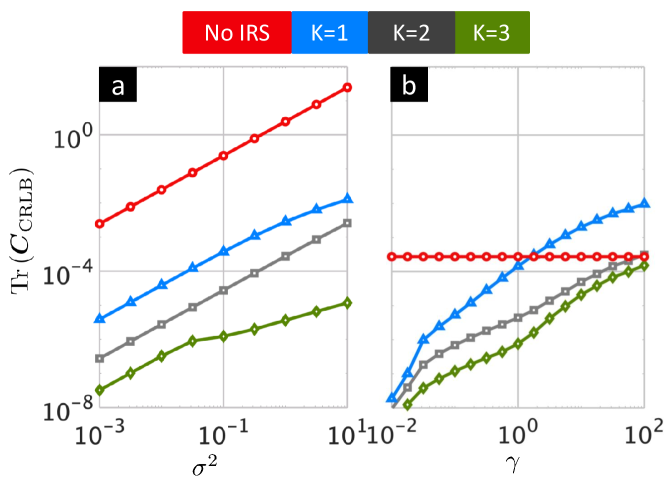
Figure 2: The CRLB of the target back-scattering coefficients and Doppler shifts for different values of (a) $\sigma^{2}\in[10^{-3},10^{1}]$ and $\gamma=0.1$, and (b) $\gamma\in[10^{-2},10^{2}]$ and $\sigma^{2}=0.1$.

Throughout all numerical experiments, the radar and target were positioned at, respectively, [$0$ m, $0$ m] and [$0$ m, $5000$ m] in the 2-D Cartesian plane. The target’s normalized Doppler shifts were drawn from the uniform distribution in the interval [0.1,0.3) with mean 0.2. We considered the distance dependent LoS path loss $h_{{}_{{\textrm{LoS}}}}=L_{0}(\frac{d}{d_{0}})^{-\beta_{0}}$, where $L_{0}=-30$ dB is the path loss at the reference distance $d_{0}=1$ m and the path-loss exponent is set as $\beta_{0}=2.5$. The NLoS path loss is set proportionally according to LoS-to-NLoS LSR $\gamma$. We positioned a single IRS platform in [$2500$ m, $2500$ m]. Next, we positioned the second and third IRS platforms in [-$2500$ m, $2500$ m] and [$0$ m, $2500$ m], respectively. For a point like target, given the radar, target and IRS positions, the corresponding radar–IRS_k and target–IRS_k angles $\theta_{ir,k}$ and $\theta_{ti,k}$, for $k\in\{1,\ldots,K\}$ are calculated geometrically in the 2-D plane. In all our experiments in order to control the LoS-to-NLoS LSR $\gamma$, the complex target reflectivity coefficients in $\boldsymbol{\alpha}$ were sampled from independent circularly symmetric complex Gaussian distribution with zero mean and variance of unity and scaled such that we have $|\alpha_{{}_{0}}h_{{}_{{\textrm{LoS}}}}|^{2}=\gamma$ and $\sum_{k=1}^{K}|\alpha_{k}h_{{}_{{\textrm{NLoS}},k}}|^{2}=1$.

For fixed $\gamma=0.1$, Fig. 2a shows the CRLB versus the noise variance, achieved using the Doppler-aware phase shifts for IRS designed in this paper. Moreover, the effectiveness of deploying multiple IRS platforms versus the no-IRS and single-IRS deployment is illustrated. Fig. 2b compares the performance for different $\gamma\in[10^{-2},10^{2}]$. We observe that IRS deployment is effective in improving estimation accuracy when $\gamma$ decreases to values below $1$, whereas deploying more than one IRS can improve the estimation accuracy for all LoS-to-NLoS LSR values. Fig. 2a-b indicate that deploying multiple IRS platforms in a radar system with the optimized Doppler-aware phase shifts is beneficial in target estimation.

VI Conclusion

Drawing on the recent advances in IRS-aided communications and radar, we investigated a pulse-Doppler multi-IRS-aided radar system with the goal of improving the estimation accuracy of a moving target. We carried out the theoretical estimation accuracy based on Fisher information analysis, aimed at designing the Doppler-aware phase shifts. Our approach improves the estimation accuracy of the Doppler shifts and target complex reflectivity over a single IRS-aided radar.

References

- [1] M. D. Renzo, M. Debbah, D.-T. Phan-Huy, A. Zappone, M.-S. Alouini, C. Yuen, V. Sciancalepore, G. C. Alexandropoulos, J. Hoydis, H. Gacanin et al., “Smart radio environments empowered by reconfigurable AI meta-surfaces: An idea whose time has come,” EURASIP Journal on Wireless Communications and Networking, vol. 2019, no. 1, pp. 1–20, 2019.
- [2] J. A. Hodge, K. V. Mishra, and A. I. Zaghloul, “Intelligent time-varying metasurface transceiver for index modulation in 6G wireless networks,” IEEE Antennas and Wireless Propagation Letters, vol. 19, no. 11, pp. 1891–1895, 2020.
- [3] Q. Wu and R. Zhang, “Towards smart and reconfigurable environment: Intelligent reflecting surface aided wireless network,” IEEE Communications Magazine, vol. 58, no. 1, pp. 106–112, 2019.
- [4] C. Kumar, S. Kashyap, R. Sarvendranath, and S. K. Sharma, “On the feasibility of wireless energy transfer based on low complexity antenna selection and passive IRS beamforming,” IEEE Transactions on Communications, vol. 70, no. 8, pp. 5663–5678, 2022.
- [5] K. V. Mishra, A. Chattopadhyay, S. S. Acharjee, and A. P. Petropulu, “OptM3Sec: Optimizing multicast IRS-aided multiantenna DFRC secrecy channel with multiple eavesdroppers,” in IEEE International Conference on Acoustics, Speech and Signal Processing, 2022, pp. 9037–9041.
- [6] G. Iacovelli, A. Coluccia, and L. A. Grieco, “Channel gain lower bound for IRS-assisted UAV-aided communications,” IEEE Communications Letters, vol. 25, no. 12, pp. 3805–3809, 2021.
- [7] N. Torkzaban and M. A. A. Khojastepour, “Shaping mmwave wireless channel via multi-beam design using reconfigurable intelligent surfaces,” in IEEE Global Communications Conference Workshops, 2021, pp. 1–6.
- [8] Z. Wang, X. Mu, and Y. Liu, “STARS enabled integrated sensing and communications,” arXiv preprint arXiv:2207.10748, 2022.
- [9] T. Wei, L. Wu, K. V. Mishra, and M. B. Shankar, “IRS-aided wideband dual-function radar-communications with quantized phase-shifts,” in IEEE Sensor Array and Multichannel Signal Processing Workshop, 2022, pp. 465–469.
- [10] A. M. Elbir, K. V. Mishra, M. R. B. Shankar, and S. Chatzinotas, “The rise of intelligent reflecting surfaces in integrated sensing and communications paradigms,” arXiv preprint arXiv:2204.07265, 2022.
- [11] Z. Esmaeilbeig, K. V. Mishra, and M. Soltanalian, “IRS-aided radar: Enhanced target parameter estimation via intelligent reflecting surfaces,” in IEEE Sensor Array and Multichannel Signal Processing Workshop, 2022, pp. 286–290.
- [12] A. Aubry, A. De Maio, and M. Rosamilia, “Reconfigurable intelligent surfaces for N-LoS radar surveillance,” IEEE Transactions on Vehicular Technology, vol. 70, no. 10, pp. 10 735–10 749, 2021.
- [13] B. Watson and J. R. Guerci, Non-line-of-sight Radar. Artech House, 2019.
- [14] X. Song, J. Xu, F. Liu, T. X. Han, and Y. C. Eldar, “Intelligent reflecting surface enabled sensing: Cramér-Rao lower bound optimization,” arXiv preprint arXiv:2204.11071, 2022.
- [15] T. Wei, L. Wu, K. V. Mishra, and M. Shankar, “Multi-IRS-aided Doppler-Tolerant wideband DFRC system,” arXiv preprint arXiv:2207.02157, 2022.
- [16] S. Buzzi, E. Grossi, M. Lops, and L. Venturino, “Foundations of MIMO radar detection aided by reconfigurable intelligent surfaces,” IEEE Transactions on Signal Processing, vol. 70, pp. 1749–1763, 2022.
- [17] Z. Esmaeilbeig, A. Eamaz, K. V. Mishra, and M. Soltanalian, “Joint waveform and passive beamformer design in multi-IRS aided radar,” arXiv preprint arXiv:2210.14458, 2022.
- [18] A. Eamaz, F. Yeganegi, and M. Soltanalian, “Modified arcsine law for one-bit sampled stationary signals with time-varying thresholds,” in IEEE International Conference on Acoustics, Speech and Signal Processing, 2021, pp. 5459–5463.
- [19] K. V. Mishra and Y. C. Eldar, “Sub-Nyquist radar: Principles and prototypes,” in Compressed Sensing in Radar Signal Processing, A. D. Maio, Y. C. Eldar, and A. Haimovich, Eds. Cambridge University Press, 2019, pp. 1–48.
- [20] E. Björnson, H. Wymeersch, B. Matthiesen, P. Popovski, L. Sanguinetti, and E. de Carvalho, “Reconfigurable intelligent surfaces: A signal processing perspective with wireless applications,” IEEE Signal Processing Magazine, vol. 39, no. 2, pp. 135–158, 2022.
- [21] M. I. Skolnik, Radar handbook, 3rd ed. McGraw-Hill, 2008.
- [22] F. Liu, Y.-F. Liu, A. Li, C. Masouros, and Y. C. Eldar, “Cramér-Rao bound optimization for joint radar-communication beamforming,” IEEE Transactions on Signal Processing, vol. 70, pp. 240–253, 2021.
- [23] M. M. Naghsh, M. Soltanalian, P. Stoica, and M. Modarres-Hashemi, “Radar code design for detection of moving targets,” IEEE Transactions on Aerospace and Electronic Systems, vol. 50, no. 4, pp. 2762–2778, 2014.
- [24] E. Vargas, K. V. Mishra, R. Jacome, B. M. Sadler, and H. Arguello, “Dual-blind deconvolution for overlaid radar-communications systems,” arXiv preprint arXiv:2208.04381, 2022.
- [25] W. J. Bangs II, “Array processing with generalized beam-formers,” Ph.D. dissertation, Yale University, 1971.
- [26] P. Stoica and R. L. Moses, Spectral analysis of signals. Prentice Hall, 2005.
- [27] S. M. Kay, Fundamentals of statistical signal processing: Estimation theory. Prentice-Hall, Inc., 1993.
- [28] R. Bamler, “Doppler frequency estimation and the cramer-rao bound,” IEEE Transactions on Geoscience and Remote Sensing, vol. 29, no. 3, pp. 385–390, 1991.
- [29] A. Eamaz, F. Yeganegi, and M. Soltanalian, “One-bit phase retrieval: More samples means less complexity?” arXiv preprint arXiv:2203.08982, 2022.
- [30] Z. Esmaeilbeig, S. Khobahi, and M. Soltanalian, “Deep-RLS: A model-inspired deep learning approach to nonlinear PCA,” arXiv preprint arXiv:2011.07458, 2020.
- [31] E. Tohidi, M. Coutino, S. P. Chepuri, H. Behroozi, M. M. Nayebi, and G. Leus, “Sparse antenna and pulse placement for colocated MIMO radar,” IEEE Transactions on Signal Processing, vol. 67, no. 3, pp. 579–593, 2018.
- [32] B.-Z. Bobrovsky, E. Mayer-Wolf, and M. Zakai, “Some classes of global cramér-Rao bounds,” The Annals of Statistics, pp. 1421–1438, 1987.
- [33] M. S. Bazaraa, H. D. Sherali, and C. M. Shetty, Nonlinear programming: Theory and algorithms. John Wiley & Sons, 2013.
- [34] J. C. Bezdek and R. J. Hathaway, “Convergence of alternating optimization,” Neural, Parallel & Scientific Computations, vol. 11, no. 4, pp. 351–368, 2003.