Flexible Modeling of Nonstationary Extremal Dependence Using Spatially-Fused LASSO and Ridge Penalties

Abstract

Statistical modeling of a nonstationary spatial extremal dependence structure is challenging. Parametric max-stable processes (MSPs) are common choices for modeling spatially-indexed block maxima, where an assumption of stationarity is usual to make inference feasible. However, this assumption is unrealistic for data observed over a large or complex domain. We develop a computationally-efficient method for estimating extremal dependence using a globally nonstationary but locally-stationary MSP construction, with the spatial domain divided into a fine grid of subregions, each with its own dependence parameters. We use LASSO ($L_{1}$) or ridge ($L_{2}$) penalties to obtain spatially-smooth parameter estimates. We then develop a novel data-driven algorithm to merge homogeneous neighboring subregions. The algorithm facilitates model parsimony and interpretability. To make our model suitable for high-dimensional data, we exploit a pairwise likelihood to perform inference and discuss its computational and statistical efficiency. We apply our proposed method to model monthly maximum temperature data at over 1400 sites in Nepal and the surrounding Himalayan and sub-Himalayan regions; we show significant improvements in model fit compared to a stationary model. Furthermore, we demonstrate that the estimated merged partition is interpretable from a geographic perspective and leads to better model diagnostics by adequately reducing the number of parameters.

Keywords: domain partitioning, max-stable process, nonstationary extremal dependence, regularization, spatial extremes.

1 Introduction

Over the past decades, various parametric max-stable processes (MSPs) have been proposed (see, e.g., Brown and Resnick, 1977; Smith, 1990; Schlather, 2002; Reich and Shaby, 2012; Opitz, 2013), among which the extremal-$t$ and Brown–Resnick classes are considered to be the most flexible. Most classical applications of MSPs assume stationarity and isotropy for simplicity and computational feasibility. Such a simplification may be unrealistic when we obtain the data over a large or complex geographical domain. Misspecification of the extremal dependence structure may cause issues for model fitting and estimation of spatial risk measures (e.g., quantiles of some spatially aggregated quantity); see Huser and Genton (2016). Therefore, building flexible models that can capture nonstationary extremal dependence is crucial.

To capture nonstationary extremal dependence, Blanchet and Davison (2011) suggest splitting the study domain into distinct subregions and fitting separate stationary extremal dependence models within each subregion, yielding a process that is inconsistent at the subregion boundaries. Locally-stationary processes are also used in the geostatistical literature by Fuentes (2001, 2002) and Muyskens et al. (2022). Based on the Bayesian information criterion or likelihood ratio test, these authors also propose a subregion-merging procedure to define the boundaries of the local processes. Such models can parsimoniously capture global nonstationarity. Alternatively, the spatial deformation approach, advocated by Sampson and Guttorp (1992) in the geostatistical literature and by Richards and Wadsworth (2021) in the spatial extremes literature, maps the original spatial locations onto a latent space, where an assumption of stationarity and isotropy is reasonable. However, the estimation and interpretation of this deformed space can be challenging. A simpler approach is to define the latent space based on covariates, such as climate variables, rather than estimating it (Cooley et al., 2007); this method strongly relies on the choice of covariates for the latent space. Another way of modeling nonstationary extremal dependence is to define a stationary model on an expanded space through multidimensional scaling (Chevalier et al., 2021), but computations and interpretation may be tricky.

In the classical spatial statistics setting, Parker et al. (2016) adopt a local stationarity perspective, and propose a computationally-efficient method for modeling global nonstationary spatial dependence using Gaussian processes (GPs) by first partitioning the domain of interest into a fine grid of subregions and assigning to each its own set of covariance parameters, then combined into a global model through the nonstationary covariance function proposed by Paciorek and Schervish (2006). Their method fixes the subregion partition and fits an overdetermined model to data, with LASSO regularization utilized to reduce the number of parameters. These penalties are also used by Sass et al. (2021) in the extremes context to regularize nonstationary marginal parameters and return levels. For extremal-$t$ MSPs, Huser and Genton (2016) extend the correlation function proposed by Paciorek and Schervish (2006) to incorporate covariates and model nonstationary spatial extremal dependence, but their approach is fairly rigid and relies on strong assumptions about the effect of specific covariates on the extremal dependence structure. By contrast, our proposed approach merges ideas from classical geostatistics and extreme value theory by developing a computationally-efficient model that can flexibly capture global nonstationarity in the extremal dependence with locally stationary subdomains. Specifically, our proposed methodology relies on MSPs and domain partitioning, akin to Parker et al. (2016), and then the efficient merging of subregions with similar parameter values in a data-driven way. While we constrain our focus to the Brown–Resnick model in this work, extensions to other MSPs are straightforward. Our proposed method also bears similarities with the local likelihood approach advocated by Castro-Camilo and Huser (2020) for modeling threshold exceedances, although we here focus on modeling maxima through max-stable processes instead and, unlike Castro-Camilo and Huser (2020), our approach takes advantage of the whole dataset at once for estimating the nonstationary spatial dependence structure.

The full-likelihood for MSPs is intractable when the dimension of data exceeds $D=13$ (Castruccio et al., 2016; Huser et al., 2019), and the analytical expression of the multivariate density is only available for a small collection of parametric models. Pairwise and triplewise likelihoods are commonly used to perform inference after being carefully studied by Padoan et al. (2010) and Huser and Davison (2013), with the latter concluding that triplewise likelihood inference has only moderate improvements over the pairwise variant. Similarly, Huser et al. (2022) adopt the Vecchia likelihood approximation technique (Vecchia, 1988; Stein et al., 2004), originally proposed in the classical geostatistical literature, in the context of spatial extremes analysis with MSPs. Alternatively, several recent works (Gerber and Nychka, 2021; Lenzi et al., 2021; Sainsbury-Dale et al., 2022) focus on estimating the spatial dependence structures using artificial neural networks in the context of both classical geostatistics and spatial extremes. However, both the Vecchia method and neural estimation are impractical in our context. The Vecchia method for spatial extremes can indeed still be relatively computationally intensive in high dimensions when using component likelihoods beyond the pairwise case, and a faster estimation technique is necessary for our iterative merging procedure, while neural estimation is also infeasible due to the large number of parameters in our model; we would need to train many neural networks with different architectures sequentially due to the nature of the merging algorithm, which would be inefficient. Hence, we prefer to use a pairwise likelihood for inference, which is both simple and quite fast. Huser and Genton (2016) suggest a careful choice of a small fraction of observation pairs for achieving computational and statistical efficiency, and we investigate this thoroughly.

The paper is organized as follows. In Section 2, we provide a brief summary of MSPs along with details of the pairwise likelihood approach to inference. Besides the nonstationary Brown–Resnick model, we discuss the computational and statistical efficiency of our pairwise likelihood approach, along with our approach to merge subregions without expert knowledge in Section 3. We illustrate the efficacy of our approach with a simulation study in Section 4 and apply our proposed methodology to Nepalese temperature data in Section 5. Section 6 concludes with a discussion of avenues for future research.

2 Max-Stable Processes

2.1 Construction

Suppose that $\{X_{i}(\bm{s}):i=1,\ldots,m\}$ are independent and identically distributed (i.i.d.) random processes with continuous sample paths on $\mathcal{S}\subset\mathbb{R}^{2}$, and that there exist sequences of functions $\alpha_{m}(\bm{s})>0$ and $\beta_{m}(\bm{s})$ such that the renormalized process of pointwise maxima $\alpha_{m}(\bm{s})^{-1}[\max\{X_{1}(\bm{s}),\ldots,X_{m}(\bm{s})\}-\beta_{m}(\bm{s})]$ converges weakly, as $m\rightarrow\infty$, to a process $\{Z(\bm{s}),\bm{s}\in\mathcal{S}\}$ with non-degenerate margins. Then $Z(\bm{s})$ is a max-stable process, and its margins follow the generalized extreme value distribution, denoted by $\operatorname{GEV}\{\mu(\bm{s}),\varsigma(\bm{s}),\xi(\bm{s})\}$, with distribution function

$$G_{\bm{s}}(z)=\exp\left(-\left[1+\xi(\bm{s})\left\{\dfrac{z-\mu(\bm{s})}{\varsigma(\bm{s})}\right\}\right]^{-1/\xi(\bm{s})}_{+}\right),$$ (1)

defined on $\{z\in\mathbb{R}:1+\xi(\bm{s})\{z-\mu(\bm{s})\}/\varsigma(\bm{s})\geq 0\}$, $a_{+}=\max(0,a)$, and where $\mu(\bm{s})\in\mathbb{R}$, $\varsigma(\bm{s})>0$, and $\xi(\bm{s})\in\mathbb{R}$ are site-dependent location, scale, and shape parameters, respectively. Consider the standardized processes $Y_{i}(\bm{s})=[1-F_{\bm{s}}\{X_{i}(\bm{s})\}]^{-1}$, $i=1,\ldots,m$, with $F_{\bm{s}}(\cdot)$ being the marginal distribution function of $X_{i}(\bm{s})$. The limiting process of renormalized maxima $\max\{Y_{1}(\bm{s}),\ldots,Y_{m}(\bm{s})\}/m$ is a MSP with unit Fréchet margins, i.e., $\operatorname{GEV}(1,1,1)$. Following de Haan (1984) and de Haan and Ferreira (2007), under mild conditions any MSP $\{Z(\bm{s}):\bm{s}\in\mathcal{S}\}$ with unit Fréchet margins can be expressed as

$$Z(\bm{s})=\sup_{i\geq 1}W_{i}(\bm{s})/P_{i},$$ (2)

where for all $i\in\mathbb{N}$, $P_{i}$ are points of a Poisson process on $(0,\infty)$ with unit rate intensity, and $\{W_{i}(\bm{s}):\bm{s}\in\mathcal{S}\}$ are i.i.d. copies of a non-negative stochastic process satisfying $\mathbb{E}\{W(\bm{s})\}=1$. The $D$-dimensional joint distribution of $Z$ at the sites $\bm{s}_{1},\ldots,\bm{s}_{D}\in\mathcal{S}$ is

$$\operatorname{Pr}\left\{Z\left(\bm{s}_{1}\right)\leq z_{1},\ldots,Z\left(\bm{s}_{D}\right)\leq z_{D}\right\}=\exp\left\{-V\left(z_{1},\ldots,z_{D}\right)\right\},$$ (3)

where the exponent function $V$ is

$$V\left(z_{1},\ldots,z_{D}\right)=\mathbb{E}\left[\max\left\{\dfrac{W\left(\bm{s}_{1}\right)}{z_{1}},\ldots,\dfrac{W\left(\bm{s}_{D}\right)}{z_{D}}\right\}\right].$$ (4)

The function $V$ has an explicit form only for specific choices of $W(\bm{s})$ with one such example arising from the construction of the Brown–Resnick model (see Section 2.2).

To measure extremal dependence between the process observed at any two sites $\bm{s}_{i}$ and $\bm{s}_{j}$, where $i,j\in\{1,\ldots,D\}$, we can use the extremal coefficient $\theta(\bm{s}_{i},\bm{s}_{j})=V_{(\bm{s}_{i},\bm{s}_{j})}(1,1)\in[1,2]$ (Schlather and Tawn, 2003), where $V_{(\bm{s}_{i},\bm{s}_{j})}$ denotes the restriction of the $D$-variate function $V$ to the variables at sites $\bm{s}_{i}$ and $\bm{s}_{j}$ only. The case $1\leq\theta(\bm{s}_{i},\bm{s}_{j})<2$ corresponds to asymptotic dependence with increasing strength of dependence as $\theta$ decreases, and $\theta(\bm{s}_{i},\bm{s}_{j})=2$ corresponds to perfect independence between limiting block maxima $Z(\bm{s}_{i})$ and $Z(\bm{s}_{j})$. The $F$-madogram (Cooley et al., 2006), defined by

$$\nu(\bm{s}_{i},\bm{s}_{j})=\dfrac{1}{2}\mathbb{E}[|F\{Z(\bm{s}_{i})\}-F\{Z(\bm{s}_{j})\}|],$$

where $F(\cdot)$ here denotes the standard Fréchet distribution function, can be used to estimate the extremal coefficient, $\theta(\bm{s}_{i},\bm{s}_{j})=\frac{1+2\nu(\bm{s}_{i},\bm{s}_{j})}{1-2\nu(\bm{s}_{i},\bm{s}_{j})}$; the empirical counterpart $\widetilde{\nu}(\bm{s}_{i},\bm{s}_{j})$ can be obtained by replacing expectations by sample averages, $F$ by the empirical CDF, and $Z$ by independent replicates of the MSP at those sites. The empirical extremal coefficient can thus naturally be defined as $\widetilde{\theta}(\bm{s}_{i},\bm{s}_{j})=\frac{1+2\widetilde{\nu}(\bm{s}_{i},\bm{s}_{j})}{1-2\widetilde{\nu}(\bm{s}_{i},\bm{s}_{j})}$.

2.2 Brown–Resnick Model

Brown and Resnick (1977) and Kabluchko et al. (2009) propose the Brown–Resnick (BR) process, defined by specifying $W(\bm{s})=\exp\{\epsilon(\bm{s})-\sigma^{2}(\bm{s})/2\}$ in (2), for a zero-mean Gaussian process $\{\epsilon(\bm{s}):\bm{s}\in\mathcal{S}\}$ with variance $\sigma^{2}(\bm{s})$ at location $\bm{s}\in\mathcal{S}$ and semivariogram $\gamma(\cdot,\cdot):\mathcal{S}\times\mathcal{S}\rightarrow[0,\infty)$. The bivariate exponent function defined in (4) is

$$V_{(\bm{s}_{i},\bm{s}_{j})}\left(z_{i},z_{j}\right)=\dfrac{1}{z_{i}}\Phi\left\{\dfrac{a}{2}-\dfrac{1}{a}\log\left(\dfrac{z_{i}}{z_{j}}\right)\right\}+\dfrac{1}{z_{j}}\Phi\left\{\dfrac{a}{2}-\dfrac{1}{a}\log\left(\dfrac{z_{j}}{z_{i}}\right)\right\},$$ (5)

with $a=\sqrt{2\gamma(\bm{s}_{i},\bm{s}_{j})}$ and where $\Phi$ is the standard Normal distribution function. Here we use the notation $\gamma(\bm{s}_{i},\bm{s}_{j})$ as the semivariogram may be nonstationary, i.e., a function of both $\bm{s}_{i}$ and $\bm{s}_{j}$ rather than their distance. The theoretical extremal coefficient for the BR model is

$$\theta\left(\bm{s}_{i},\bm{s}_{j}\right)=V_{(\bm{s}_{i},\bm{s}_{j})}(1,1)=2\Phi\left[\dfrac{\left\{2\gamma(\bm{s}_{i},\bm{s}_{j})\right\}^{1/2}}{2}\right],$$ (6)

where $\gamma(\bm{s}_{i},\bm{s}_{j})$ controls the strength and decay of dependence within the process.

2.3 Composite Likelihood Inference

Full likelihood inference for max-stable processes observed at a large number of sites is computationally expensive, as evaluation of the $D$-dimensional joint density involves the differentiation of (3) with respect to $z_{1},\ldots,z_{D}$, which leads to a summation indexed by all possible partitions of $\{1,\ldots,D\}$. The number of terms grows at a sup-exponential rate with $D$. More precisely, the full $D$-dimensional density is computationally intractable even for moderate $D$, i.e., $D>12$ (Padoan et al., 2010; Castruccio et al., 2016; Huser et al., 2019). To tackle this issue, (composite) pairwise likelihood (PL) inference is often used in practice. Denoting $z_{t,i}$ as the $t$-th block maxima recorded at $\bm{s}_{i}$ for $t=1,\ldots,T$ and $i=1,\ldots,D$, the pairwise log-likelihood $\ell_{PL}$ with $p$-dimensional parameter set $\bm{\psi}$ is

$$\ell_{PL}(\bm{\psi})=\sum^{T}_{t=1}\sum_{(i,j)\in\mathcal{O}}\left[\log\left\{V_{i}(z_{t,i},z_{t,j})V_{j}(z_{t,i},z_{t,j})-V_{ij}(z_{t,i},z_{t,j})\right\}-V_{(\bm{s}_{i},\bm{s}_{j})}(z_{t,i},z_{t,j})\right],$$ (7)

where $V_{i}=\frac{\partial V_{(\bm{s}_{i},\bm{s}_{j})}}{\partial z_{i}}$ and $V_{ij}=\frac{\partial^{2}V_{(\bm{s}_{i},\bm{s}_{j})}}{\partial z_{i}\partial z_{j}}$, and the function arguments have been omitted for simplicity, and $\mathcal{O}\subset\mathcal{O}_{total}$ with $\mathcal{O}_{total}=\{(i,j):1\leq i<j\leq D\}$ taken to be all unique pairs of site indices. If $\mathcal{O}=\mathcal{O}_{total}$, all available observation pairs are utilized and this leads to inefficient inference due to the use of redundant information. Therefore, a careful choice of a significantly smaller number of pairs is suggested by Huser and Genton (2016) to achieve computational and statistical efficiency. A possibility is to include a small fraction of strongly dependent pairs (Bevilacqua et al., 2012), i.e., the closest ones in the stationary and isotropic case, or using more distant pairs of sites (Huser (2013), Chapter 3; Huser and Davison (2014)). For a nonstationary model, selecting pairs using the lowest pre-computed empirical extremal coefficients, i.e., the ones estimated with the strongest dependence, leads to bias in parameter estimates (Huser and Genton, 2016); instead of sampling only the closest observation pairs, we want to include pairs with various distances to fully explore the extremal dependence structure. To this end, we propose two strategies: a simple and a stratified sampling scheme. Our simple strategy is to randomly sample a small fraction of observation pairs with uniform probability from all those available. With stratified sampling, we stratify observation pairs into predefined distance classes, and then draw the same percentage of pairs from each class; this approach ensures that the distribution of distances among sampled pairs is approximately uniform so that the distant pairs have a similar “weight” in the pairwise likelihood compared to the close pairs. Our simulations in Section 4.2 investigate the statistical efficiency of both sampling schemes.

Assuming independence between temporal replicates, the maximum pairwise likelihood estimator, denoted $\hat{\bm{\psi}}$, is generally asymptotically Gaussian with convergence rate $\sqrt{T}$. Specifically, if $\bm{\psi}_{0}$ is the true parameter vector, then under mild regularity conditions the distribution of $\hat{\bm{\psi}}$ for large $T$ is $\hat{\bm{\psi}}\overset{\cdot}{\sim}\textrm{Normal}\left(\bm{\psi}_{0},\bm{J}(\bm{\psi}_{0})^{-1}\bm{K}(\bm{\psi}_{0})\bm{J}(\bm{\psi}_{0})^{-1}\right)$, where $\bm{J}(\bm{\psi})=\mathbb{E}\{-\partial^{2}\ell_{PL}(\bm{\psi})/(\partial\bm{\psi}\partial\bm{\psi}^{T})\}\in\mathbb{R}^{p\times p}$ and $\bm{K}(\bm{\psi})=\operatorname{Var}\{\partial\ell_{PL}(\bm{\psi})/\partial\bm{\psi}\}\in\mathbb{R}^{p\times p}$ are the (pairwise) expected information matrix and variance of the score function, respectively. Evaluating $\bm{J}(\bm{\psi})$ and $\bm{K}(\bm{\psi})$ at an estimate $\hat{\bm{\psi}}$, we can obtain the approximate asymptotic variance of $\hat{\bm{\psi}}$. Model selection in this composite likelihood framework may be performed using either the composite likelihood information criterion (CLIC) or the composite Bayesian information criterion (CBIC), defined by $\operatorname{CLIC}=-2\ell_{PL}(\hat{\bm{\psi}})+2\operatorname{tr}\{\bm{J}(\hat{\bm{\psi}})^{-1}\bm{K}(\hat{\bm{\psi}})\}$, and $\operatorname{CBIC}=-2\ell_{PL}(\hat{\bm{\psi}})+\log(T)\operatorname{tr}\{\bm{J}(\hat{\bm{\psi}})^{-1}\bm{K}(\hat{\bm{\psi}})\}$, respectively, where a model with a lower CLIC or CBIC value is preferred (Ng and Joe, 2014).

3 Methodology

3.1 Nonstationary Variogram for Brown–Resnick Model

Similarly to Huser and Genton (2016), we model nonstationarity in extremal dependence by combining the BR max-stable process with a nonstationary exponential variogram constructed using a convolution-based nonstationary covariance model (Paciorek and Schervish, 2006). We begin by writing the variogram as

$$2\gamma(\bm{s}_{i},\bm{s}_{j})=\operatorname{Var}\{\epsilon(s_{i})-\epsilon(s_{j})\}=\operatorname{Var}\{\epsilon(\bm{s}_{i})\}+\operatorname{Var}\{\epsilon(\bm{s}_{j})\}-2\operatorname{Cov}\{\epsilon(\bm{s}_{i}),\epsilon(\bm{s}_{j})\}.$$ (8)

We then allow $\operatorname{Cov}(\cdot,\cdot)$ to be the nonstationary covariance function

$$\operatorname{Cov}\{\epsilon(\bm{s}_{i}),\epsilon(\bm{s}_{j})\}=\sigma\left(\bm{s}_{i}\right)\sigma\left(\bm{s}_{j}\right)\rho\left(\bm{s}_{i},\bm{s}_{j}\right),$$ (9)

where $\sigma(\bm{s})>0$ is a location-dependent sill parameter and $\rho\left(\bm{s}_{i},\bm{s}_{j}\right):\mathcal{S}\times\mathcal{S}\rightarrow[0,1]$ is a nonstationary (positive definite) correlation function. Although other choices are possible, we here define $\rho$ in terms of a stationary isotropic exponential correlation function $\rho^{*}(h)=\exp(-h)$, for $h\geq 0$, as

$$\rho\left(\bm{s}_{i},\bm{s}_{j}\right)=\left|\bm{\Omega}\left(\bm{s}_{i}\right)\right|^{\frac{1}{4}}\left|\bm{\Omega}\left(\bm{s}_{j}\right)\right|^{\frac{1}{4}}\left|\dfrac{\bm{\Omega}\left(\bm{s}_{i}\right)+\bm{\Omega}\left(\bm{s}_{j}\right)}{2}\right|^{-\frac{1}{2}}\rho^{*}\left(d_{ij}\right),$$ (10)

with $\bm{\Omega}\left(\bm{s}\right)$ a location-dependent $2\times 2$ positive definite kernel matrix controlling the range and shape of local dependence at $\bm{s}$, and where $d_{ij}$ is the Mahalanobis distance between sites, with the form $d_{ij}=\left[\left(\bm{s}_{i}-\bm{s}_{j}\right)^{T}\left\{\dfrac{\bm{\Omega}\left(\bm{s}_{i}\right)+\bm{\Omega}\left(\bm{s}_{j}\right)}{2}\right\}^{-1}\left(\bm{s}_{i}-\bm{s}_{j}\right)\right]^{1/2}$. Here, we focus on the locally isotropic case, for which $\bm{\Omega}\left(\bm{s}\right)=\phi(\bm{s})\bm{I}_{2}$, where $\phi(\bm{s})\geq 0$ is a location-dependent range parameter. More complex non-isotropic cases are possible with general covariance matrices $\bm{\Omega}(\bm{s})$. Substituting (9) into (8) yields the nonstationary exponential variogram $2\gamma(\bm{s}_{i},\bm{s}_{j})=\sigma^{2}\left(\bm{s}_{i}\right)+\sigma^{2}\left(\bm{s}_{j}\right)-2\sigma\left(\bm{s}_{i}\right)\sigma\left(\bm{s}_{j}\right)\rho\left(\bm{s}_{i},\bm{s}_{j}\right)$, which can be used into (5) for constructing nonstationary BR processes.

3.2 Domain Partitioning and Parameter Regularization

To reduce the number of parameters that are needed to represent the dependence structure, we partition the whole domain into a base partition $\mathcal{P}$ which consists of $R$ subregions $\{\mathcal{R}_{1},\mathcal{R}_{2},\ldots,\mathcal{R}_{R}\}$. This partition should be constructed to compromise parameter estimation accuracy and model flexibility. If the subregions are too small, the estimation of parameters in each subregion can be numerically unstable; if subregions are too large, the model may be incapable of capturing fine-scale nonstationarity in the extremal dependence. Similarly to Parker et al. (2016), we impose a penalty to regularize the dependence parameters and fit the model by maximizing the penalized pairwise log-likelihood (PPL)

$$\ell_{PPL}(\bm{\psi})=\ell_{PL}(\bm{\psi})-\sum_{i=1}^{2}\lambda_{i}\sum_{r_{1}\sim r_{2}}\left|\psi_{ir_{1}}-\psi_{ir_{2}}\right|^{q},$$ (11)

where $\psi_{1r}=\log(\sigma^{2}_{r})$ and $\psi_{2r}=\log(\phi_{r})$ are the log-transformed sill and range parameters, respectively, for subregion $\mathcal{R}_{r}$, and the operation $r_{1}\sim r_{2}$ refers to neighboring subregions $\mathcal{R}_{r_{1}},\mathcal{R}_{r_{2}}$, sharing a common boundary. Equation (11) with $q=1$ and $q=2$ corresponds to LASSO ($L_{1}$) and ridge ($L_{2}$) regularization, respectively. Both LASSO and ridge regularization enforce spatial “smoothness” in the dependence parameters, but in different ways: while the LASSO regularization penalizes more small discrepancies (and can even enforce parameters in neighboring subregions to be equal), the ridge regularization penalizes more large discrepancies and tends to produce parameter surfaces that are smoother overall.

Instead of fixing the domain partition as Parker et al. (2016), we iteratively update the partition $\mathcal{P}$ and reduce the number of parameters required for our model. Alongside increased parsimonity, this approach allows us to better identify stationary subdomains of $\mathcal{S}$, which also leads to easier model interpretation. We achieve this in a data-driven way, without the need for domain knowledge or covariate information. Our strategy is to start with a fine collection of subregions as a base partition and then iteratively update the partition by merging neighboring subregions, according to some quantifiable improvement in model fit.

Starting with the base partition, denoted $\mathcal{P}^{0}$, a new partition $\mathcal{P}^{j}$ is generated by merging neighboring subregions at subsequent steps $j=1,2,3,\ldots$, according to some criteria. Different criteria have been proposed, including the BIC (Fuentes, 2001) and deviance (Muyskens et al., 2022), but these approaches are not applicable when the likelihood is penalized. Instead, we select a partition using the PPL, computed over a single holdout set $\bm{z}_{\mathrm{hold}}$. We denote this $\ell_{PPL}(\hat{\bm{\psi}};\bm{z}_{\mathrm{hold}})$, where the estimate $\hat{\bm{\psi}}$ maximizes $\ell_{PPL}$ on a training set $\bm{z}_{\mathrm{train}}$. We can also use the average holdout PPL over data folds, which involves a higher computational burden but a more stable model fitting. We take this approach in our data application. The penalty term in (11) inherently includes information about the number of parameters in the model, with the total number of neighboring subregion pairs, i.e., the number of model parameters, reducing whenever some subregions merge. By selecting the model with the larger PPL, we balance model flexibility and parsimony.

To choose candidate subregions to merge at step $j$, Muyskens et al. (2022) suggest randomly sampling neighboring pairs from all available neighboring subregions, and testing a merge; this is performed exhaustively, without replacement, until acceptance. We instead merge all neighboring pairs of subregions with estimated parameter difference $d(\hat{\bm{\psi}}^{j-1}_{r_{1}},\hat{\bm{\psi}}^{j-1}_{r_{2}})>0$ smaller than some predefined threshold $\eta^{j}>0$, which is dependent on step $j$. This procedure allows us to reduce computational time by merging multiple subregions simultaneously. At step $j$, we choose a sequence of descending candidate thresholds $\bm{\mathcal{H}}^{j}=\{\eta^{j}_{1:H}:\eta^{j}_{1}>\cdots>\eta^{j}_{H}\}$, where $H=H(j)\in\mathbb{N}_{+}$ that may change with iteration $j$. We start by generating a candidate for the next partition $\mathcal{P}^{j}$ by merging all neighboring pairs of subregions with estimated parameter difference smaller than $\eta^{j}_{1}$. If the model fitted with this candidate partition increases the holdout PPL, then the candidate partition is accepted for $\mathcal{P}^{j}$. Otherwise, we create a new candidate similarly using the smaller threshold $\eta^{j}_{h}$ and repeat this procedure, for all $h$. If no improvement is observed using the final threshold in $\bm{\mathcal{H}}^{j}$, the procedure stops and the final partition $\hat{\mathcal{P}}$ is $\mathcal{P}^{j-1}$.

The number of subregions in the final partition $\hat{\mathcal{P}}$ is of interest. As we take a data-driven approach, the final partition $\hat{\mathcal{P}}$ may be sensitive to the choice of holdout set and observation pairs used for optimization. Hence, we advocate estimation of a number of different $\hat{\mathcal{P}}$ using different holdout sets and observation pairs, and selecting the most reasonable.

We tune $\bm{\lambda}=(\lambda_{1},\lambda_{2})$ using a similar approach to Parker et al. (2016). For the initial partition $\mathcal{P}^{0}$, we begin with the fully stationary model, i.e., with $\lambda_{1}=\lambda_{2}=\infty$, and then iteratively fit two models with new $\bm{\lambda}$ values. Each time $\bm{\lambda}$ is updated according to descending grids $\bm{\Lambda}^{0}_{i}=\{\infty,\lambda^{0}_{i,2},\ldots,\lambda^{0}_{i,K^{0}_{i}}\}$ for $i=1,2$, until acquiring an optimal selection, denoted $\hat{\bm{\lambda}}^{0}$. Specifically, two different models are fitted, one with $(\lambda^{0}_{1,2},\infty)$ and one with $(\infty,\lambda^{0}_{2,2})$. If a larger pairwise log-likelihood on the holdout set is achieved by one of them, we choose the model with the largest improvement. We repeat this procedure until there is no improvement. As $\bm{\lambda}$ controls model complexity, it should vary with the partition, and so we tune $\bm{\lambda}$ for each new partition $\mathcal{P}^{j}$, yielding the sequence of penalty parameters $\hat{\bm{\lambda}}^{j}$ for step $j$. We denote by $\hat{\bm{\lambda}}$ the estimated penalty parameter $\bm{\lambda}$ for the final estimated partition $\hat{\mathcal{P}}$. After tuning $\bm{\lambda}$, the PPL is calculated on the holdout sets and used for selecting a new partition. We describe the selection of candidate thresholds $\bm{\mathcal{H}}$ and the descending grid $\bm{\Lambda}=\{\bm{\Lambda}_{1},\bm{\Lambda}_{2}\}$ in Section LABEL:Supp:MASDiag of supplementary materials. The full algorithm for estimating $\hat{\mathcal{P}}$ is detailed in Algorithm 1.

input : Base partition $\mathcal{P}^{0}=\{r_{1},\ldots,r_{R^{0}}\}$, descending grid $\bm{\Lambda}^{0}$, a holdout set $\bm{z}_{\mathrm{hold}}$

output : A final partition $\hat{\mathcal{P}}$

$\hat{\bm{\lambda}}^{0},\ell_{PPL}^{0}(\bm{z}_{\mathrm{hold}};\hat{\bm{\psi}}^{0},\bm{z}_{\mathrm{train}})\leftarrow$ LambdaTuning($\mathcal{P}^{0}$, $\bm{\Lambda}^{0}$, $\bm{\lambda}^{0}$);

$j\leftarrow 1$ ;

  /* Iteration $j$. */

repeat

       $\bm{\lambda}^{j}\leftarrow\hat{\bm{\lambda}}^{j-1}$;

       $\bm{\Lambda}^{j}\leftarrow$ UpdateGrid($\hat{\bm{\lambda}}^{j-1}$, $\bm{\lambda}^{j-1}$, $\bm{\Lambda}^{j-1}$);

       Calculate $\{d(\hat{\bm{\psi}}^{j-1}_{r_{1}},\hat{\bm{\psi}}^{j-1}_{r_{2}}):r_{1}\sim r_{2},r_{1},r_{2}=1,\ldots,R^{j-1}\}$;

       Choose $\bm{\mathcal{H}}^{j}=\{\eta^{j}_{1:H}:\eta^{j}_{1}>\cdots>\eta^{j}_{H}\}$;

       $h\leftarrow 1$ ;

        /* $h$-th element of the threshold candidates. */

       repeat

             $\eta^{j}\leftarrow\eta^{j}_{h}$;

             $r_{1}^{j}\leftarrow(r_{1}^{j-1},r_{2}^{j-1})$ if $d(\hat{\bm{\psi}}^{j-1}_{r_{1}},\hat{\bm{\psi}}^{j-1}_{r_{2}})<\eta^{j}$ & $r_{1}^{j-1}\sim r_{2}^{j-1}$ and acquire a candidate partition $\mathcal{P}^{j}_{\mathrm{cand}}=\{\mathcal{R}^{j}_{1},\ldots,\mathcal{R}^{j}_{R^{j}_{\mathrm{cand}}}\}$;

             $\hat{\bm{\lambda}}_{\mathrm{cand}}^{j},\ell_{PPL,\mathrm{cand}}^{j}(\bm{z}_{\mathrm{hold}};\hat{\bm{\psi}}^{j},\bm{z}_{\mathrm{train}})\leftarrow$ LambdaTuning($\mathcal{P}^{j}_{\mathrm{cand}}$, $\bm{\Lambda}^{j}$, $\bm{\lambda}^{j}$);

             $h\leftarrow h+1$;

            

      until $\ell_{PPL}^{j}(\bm{z}_{\mathrm{hold}};\hat{\bm{\psi}}^{j},\bm{z}_{\mathrm{train}})>\ell_{PPL}^{j-1}(\bm{z}_{\mathrm{hold}};\hat{\bm{\psi}}^{j-1},\bm{z}_{\mathrm{train}})$;

      Update $\mathcal{P}^{j}\leftarrow\mathcal{P}^{j}_{\mathrm{cand}}$; $\hat{\bm{\lambda}}^{j}\leftarrow\hat{\bm{\lambda}}_{\mathrm{cand}}^{j}$; $\ell_{PPL}^{j}(\bm{z}_{\mathrm{hold}};\hat{\bm{\psi}}^{j},\bm{z}_{\mathrm{train}})\leftarrow\ell_{PPL,\mathrm{cand}}^{j}(\bm{z}_{\mathrm{hold}};\hat{\bm{\psi}}^{j},\bm{z}_{\mathrm{train}})$;

       $j\leftarrow j+1$ ;

      

until $h=H$;

$\hat{\mathcal{P}}=\mathcal{P}^{j-1}$ ;

  /* Final merged partition. */

Algorithm 1 Partition selection and $\bm{\lambda}$ tuning

4 Simulation Study

4.1 Overview

In the simulation study, we first investigate the statistical properties of the maximum PL estimator using different proportions of pairs for inference in Section 4.2. We then study the model performance on simulated data in terms of model fit and true partition recovery in Sections 4.3 and 4.4, respectively.

We generate data on a $\mathcal{D}=40\times 40$ grid of sites in the unit square $[0,1]\times[0,1]$, thus with $D=1600$ spatial locations. We then partition $\mathcal{D}$ into four subdomains, $\mathcal{D}_{r},r=1,\ldots,4$, under two cases: i) a square grid or ii) a triangular grid, see Figure 1. Each subdomain has its own sill, $\sigma^{2}$, and range parameter, $\phi$, as defined in (10). We consider two different cases for the extremal dependence structure and enforce that only one of the two parameters varies across subregions. The other remains fixed over $\mathcal{D}=\bigcup^{4}_{r=1}\mathcal{D}_{r}$. The two cases are:

• Case 1: $\sigma^{2}$ varies with values $\{0.5,2,2,5\}$ for the subdomains $\mathcal{D}_{1}$, $\mathcal{D}_{2}$, $\mathcal{D}_{3}$, and $\mathcal{D}_{4}$, respectively, with $\phi=2$ fixed over $\mathcal{D}$.

• Case 2: $\phi$ varies with values $\{0.05,0.2,0.2,0.5\}$ for the subdomains $\mathcal{D}_{1}$, $\mathcal{D}_{2}$, $\mathcal{D}_{3}$, and $\mathcal{D}_{4}$, respectively, with $\sigma^{2}=0.2$ fixed over $\mathcal{D}$.

These two cases can help us to understand and compare the influence of each parameter on the extremal dependence structure. Approximate samples of a BR process are then generated in each case; for a single replicate, we generate $m^{*}$ independent realizations $\epsilon_{i}(\bm{s})$, $i=1,\ldots,m^{*}$, of a Gaussian process $\{\epsilon(\bm{s}):\bm{s}\in\mathcal{S}\}$ with zero mean and covariance matrix constructed using (9). Points $P_{1},\ldots,P_{m^{*}}$ are sampled independently from a unit rate Poisson point process and ordered increasingly. Setting $W_{i}(\bm{s})=\exp\{\epsilon_{i}(\bm{s})-\sigma^{2}(\bm{s})/2\}$ for $i=1,\ldots,m^{*}$, and then computing $Z(\bm{s})=\max_{1\leq i\leq m^{*}}\{W_{i}(\bm{s})/P_{i}\}$ gives an approximate realization of the target BR process. With the accuracy of the approximation increasing with $m^{*}$, we found that setting $m^{*}=10^{5}$ produced reasonable replicates of a BR process. We repeat this to obtain $T=100$ independent temporal replicates of $Z(\bm{s})$, and the overall experiment is repeated $N=100$ times to assess the performance of our estimation approach.

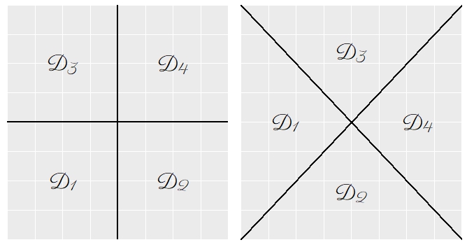
Figure 1: True partitions for simulation study. Left: true partition i), square grid; right: true partition ii), triangular grid.

4.2 Selecting Observation Pairs

Suppose $\hat{\bm{\psi}}_{\mathcal{O}}=\max_{{\bm{\psi}}_{\mathcal{O}}}\ell_{PL}(\bm{\psi};\mathcal{O})$ is the maximum pairwise likelihood estimator, evaluated using the subset of observation pairs $\mathcal{O}\subset\mathcal{O}_{\mathrm{total}}$. Using different percentages of observation pairs, varying from $0.005\%$ to $100\%$, and nonstationary data, we estimate $\hat{\bm{\psi}}_{\mathcal{O}}$ to study the variability of the estimator around the true parameter values. We select the observation pairs with the methods discussed in Section 3, i.e., simple and stratified random sampling, with the latter using ten equal-length distance classes. Nonstationary models are fitted with true partitions i) and ii), and we consider both cases 1 and 2 for parameter specification; results for true partition ii) were very similar and so we omit these for brevity. We quantify the estimation accuracy through the root mean squared error (RMSE). For example, with estimated parameter, $\hat{\sigma}^{2}_{n,r}$, and its true value, $\sigma^{2}_{r}$, for the subdomain $\mathcal{D}_{r}$ and each experiment $n=1,\ldots,N$ in case 1, we compute $\operatorname{RMSE}(\hat{\bm{\sigma}}_{n}^{2})=\sqrt{\frac{1}{4}\sum^{4}_{r=1}(\hat{\sigma}^{2}_{n,r}-\sigma^{2}_{r})^{2}}$, and similarly for the range parameter $\phi$.

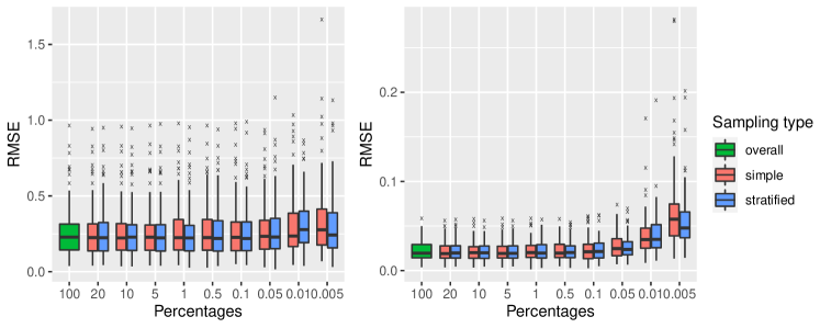
(a)

Figure 2: Boxplots of the RMSE for $\hat{\bm{\psi}}_{\mathcal{O}}$ using all observation pairs (green), the simple random sampling (red), and stratified sampling (blue) schemes. Left: case 1, varying $\sigma^{2}$; right: case 2, varying $\phi$.

Figure 2 (left and right panels) reports the RMSE boxplots for cases 1 and 2, i.e., $\operatorname{RMSE}(\hat{\bm{\sigma}}_{n}^{2})$ and $\operatorname{RMSE}(\hat{\bm{\phi}}_{n})$, respectively. We observe that there is no significant difference in the performance of different sampling strategies if more than $0.05\%$ of observation pairs are used for fitting. However, the stratified sampling scheme tends to slightly outperform the simple one when only $0.01\%$ pairs or less are available, and usually provides less biased estimates in both cases 1 and 2, especially for the estimation of the range parameter; hence we advocate using the stratified sampling method if only a small fraction of observation pairs are available for inference. In our application, we use only $0.1\%$ of observation pairs for fitting, to balance computational time and statistical efficiency. We use simple random sampling in Section 4.3, but stratified sampling in our application (see Section 5).

4.3 Model Performance

We now compare the performance of the three extremal dependence models we have discussed: a fully stationary BR model (model S), a nonstationary BR model using the base partition (Model B), and a nonstationary BR model using the fully-merged partition (Model M); in the case of Models B and M, we consider both $L_{1}$ and $L_{2}$ regularizations to optimally “smooth” parameter estimates. We simulate data with both extremal dependence cases 1 and 2 on both true partitions i) and ii).

To study the influence of base partition $\mathcal{P}^{0}$ misspecification (with respect to the true partition) on the final model fit, we consider two scenarios: one where the base partition $\mathcal{P}^{0}$ is well-specified and it is feasible to obtain $\hat{\mathcal{P}}=\mathcal{P}_{0}$, for true partition $\mathcal{P}_{0}$, and one where $\mathcal{P}^{0}$ is misspecified, i.e., $\hat{\mathcal{P}}=\mathcal{P}_{0}$ is infeasible. In both scenarios, the base partition is constructed from 100 subregions. For true partition i) (square grid), the well-specified $\mathcal{P}^{0}$ is constructed by considering a regular subgrid, whereas the misspecified $\mathcal{P}^{0}$ is generated with a $k$-means clustering algorithm using spatial coordinates as inputs, and where some subregions overlap the true boundaries. For true partition ii), we only consider a misspecified base partition constructed using a similar $k$-means algorithm. Among the $D=1600$ observation locations, $15\%$ are randomly selected as a validation set ($D_{\mathrm{valid}}=240$). For the nonstationary models, another $15\%$ locations are randomly selected as a holdout set ($D_{\mathrm{hold}}=240$) whilst ensuring that at least one location is within each subregion in the base partition.

To evaluate parameter estimation, we adopt the integrated RMSE, e.g., for the sill estimates $\hat{\bm{\sigma}}^{2}$, we have $\operatorname{IntRMSE}(\hat{\bm{\sigma}}^{2})=\sqrt{\frac{1}{N}\sum^{N}_{n=1}\frac{1}{D}\sum^{D}_{j=1}\left(\hat{\sigma}^{2}_{n}(\bm{s}_{j})-\sigma^{2}(\bm{s}_{j})\right)^{2}},$ where $\sigma^{2}(\bm{s}_{j})$ and $\hat{\sigma}_{n}^{2}(\bm{s}_{j})$ denote the true and the fitted value, respectively, for experiment $n$ at site $\bm{s}_{j}$. To assess full model fits, we compute the PL on the validation set, the PPL on the holdout set, and the CLIC and CBIC on the training set for each model. The results of our studies regarding model fit are given in Tables 1 and Tables LABEL:tab:extVaryRange and LABEL:tab:triangle in supplementary materials.

Table 1: Models’ performances for case 1 (varying $\sigma^{2}$) with true partition i). The relative factors shown in subscript parentheses highlight the ratios between the nonstationary and stationary models. In the first four rows, the value of the best model has been subtracted. The best value in each row is in bold.

	Sta.	Nonstationary
		Model B				Model M
		well-specified		misspecified		well-specified		misspecified
		$L_{1}$	$L_{2}$	$L_{1}$	$L_{2}$	$L_{1}$	$L_{2}$	$L_{1}$	$L_{2}$
PL Diff.	$-80769$	0	$-73$	$-9878$	$-9951$	$-522$	$-331$	$-11664$	$-11137$
PPL Diff.	–	$-27782$	$-27017$	$-5589$	$-1878$	$-24601$	$-24458$	$-909$	0
CLIC Diff.	$7971778$	$371200$	$30100$	$987205$	$1883071$	$46107$	0	$733784$	$686710$
CBIC Diff.	$7912086$	$896595$	$103570$	$1480716$	$3538099$	$91714$	0	$750201$	$718914$
IntRMSE $\hat{\bm{\sigma}}^{2}$	$1.65$	$0.54_{(0.33)}$	$0.54_{(0.33)}$	$0.73_{(0.44)}$	$0.73_{(0.44)}$	$0.39_{(0.23)}$	$\bm{0.36_{(0.22)}}$	$0.71_{(0.43)}$	$0.71_{(0.43)}$
IntRMSE $\hat{\bm{\phi}}$	$0.04$	$0.09_{(2.26)}$	$0.09_{(2.27)}$	$0.09_{(2.32)}$	$0.09_{(2.33)}$	$0.05_{(1.16)}$	$\bm{0.04_{(0.86)}}$	$0.06_{(1.57)}$	$0.06_{(1.54)}$

When only the sill varies (Table 1), all nonstationary models exhibit larger estimates of the PL, PPL, and lower estimates of CLIC, and CBIC than the stationary model, which indicates that the nonstationary models provide better fits as expected. Model M outperforms Model B as we observe larger PPL, and lower CLIC and CBIC. The nonstationary models provide a more accurate estimation of the spatially-varying $\sigma^{2}$ (with both penalties), observable through the reduced integrated RMSE. However, for $\phi$ estimation, some estimation accuracy is sacrificed when using nonstationary models (approximately $2.3$ times integrated RMSE for Model B, and only about 1–1.5 times for Model M, compared to the stationary model), but, from a practical standpoint, these errors are not large. It is noteworthy that nonstationary models with a misspecified base partition outperform the stationary model, which validates the efficacy of nonstationary models. We further note that Model M provides lower integrated RMSE than Model B for both the sill and range parameters, which indicates that merging subregions improves parameter estimation. In general, $L_{2}$ regularization performs better in the well-specified and misspecified cases for Model M. As expected, nonstationary models with a well-specified partition have better performance. Tables LABEL:tab:extVaryRange and LABEL:tab:triangle in the supplementary materials show the results for case 2 of the extremal dependence structure with true partition i) and both dependence cases with true partition ii), respectively. Similarly to case 1 with true partition i), we again observe that nonstationary models show their advantages in terms of both model fit and estimation of spatially-varying parameters, and Model M further generally outperforms Model B. We need to sacrifice some accuracy for the fixed parameter estimation when using nonstationary models, but Model M, compared to Model B, demonstrates ability to reduce the estimation error. In general, $L_{2}$ regularization performs better than $L_{1}$.

4.4 True Partition Recovery

To evaluate the accuracy of an estimated partition, we use the Rand index (RI). As a measure of the similarity between two data clusters, the RI is defined as the proportion of points that are correctly grouped together based on the true model partition $\mathcal{P}_{0}$ and the estimated partition $\hat{\mathcal{P}}$, i.e.,

$$\operatorname{RI}=\frac{O_{ss}+O_{dd}}{\binom{D}{2}},$$

where $O_{ss}$ ($O_{dd}$) is the number of pairs of sites that are simultaneously in the same (different) subset of both $\mathcal{P}_{0}$ and $\hat{\mathcal{P}}$. We also introduce a local Rand index (LRI) to assess the partition accuracy for each site. For each specific site $\bm{s}_{j}$, for $j=1,\ldots,D$, the $\operatorname{LRI}(\bm{s}_{j})$ is defined as

$$\operatorname{LRI}(\bm{s}_{j})=\frac{1}{T}\sum^{T}_{t=1}\frac{1}{D-1}\sum_{i\neq j}\mathbb{I}( \bm{s}_{i},\bm{s}_{j}\in\text{ the same subregion in both }\mathcal{P}_{0}\text{ and }\hat{\mathcal{P}}\text{ or }$$ (12)

$$\bm{s}_{i},\bm{s}_{j}\in\text{ different subregions in both }\mathcal{P}_{0}\text{ and }\hat{\mathcal{P}}).$$

where $\mathbb{I}(\cdot)$ denotes the indicator function. Larger values of $\operatorname{LRI}(\bm{s}_{j})$ correspond to better classification of site $\bm{s}_{j}$.

Table 2: Rand index values for the well-specified and misspecified variants of the true partition designs in Figure 1, with both choices of regularization and dependence regimes. The best value in each row and for each setting (well-specified or misspecified) is in bold.

Base partition		Well-specified			Misspecified
		Model B	Model M		Model B	Model M
			$L_{1}$	$L_{2}$		$L_{1}$	$L_{2}$
true partition i)	Case 1	0.760	0.982	0.998	0.759	0.852	0.859
(Square)	Case 2	0.760	0.954	0.964	0.759	0.832	0.838
true partition ii)	Case 1	-	-	-	0.758	0.741	0.769
(Triangular)	Case 2	-	-	-	0.758	0.787	0.790

Table 2 summarizes the performance of models in terms of their recovery of true partitions i) and ii). The results show that Model M generally outperforms Model B by providing larger RI values overall, with the $L_{2}$ regularization consistently performing better. Results in Tables 1–2 suggest that the $L_{2}$ regularization is generally preferable.

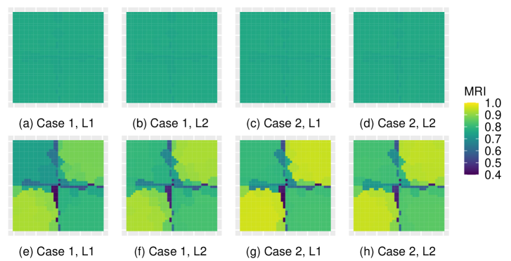
Figure 3: Average LRI for Model B (first row) and Model M (second row) for each site with true partition i) and misspecified base partition (based on $k$-means clustering).

Figures 3, LABEL:pic:LRI+well and LABEL:pic:LRIx (see supplementary materials for the latter two) give the LRI for each site for the three scenarios discussed in Section 4.3, which illustrate the performance of the merged or base partitions on each pixel in terms of region classification. Model M with a well-specified base partition generally gives the correct classification of each site as shown from the results in Figure LABEL:pic:LRI+well. When the base partition is misspecified, the merged partitions generally provide smaller LRI for the few sites lying near the boundaries of the true partition and considerably larger LRI for the many sites within the interior of the true subdomains, indicating a better classification of individual sites overall. We note that the LRI of the sites in subdomains $\mathcal{D}_{2}$ and $\mathcal{D}_{3}$ in Figure 1 are smaller than those in subdomains $\mathcal{D}_{1}$ and $\mathcal{D}_{4}$ for both true partition cases, as the parameter values in the former subdomains are here assumed to be equal and hence they are sometimes merged together by our algorithm. This affects partition estimation using Model M. However, with accurate parameter estimation, such misspecification does not impact our characterization of the extremal dependence structure, and grouping more locations with similar dependence characteristics together in the same cluster may even improve parameter estimation.

5 Nepal Temperature Data Analysis

Nepal is a south Asian country covering the Himalayan foothills and the highest peaks of the Himalayan mountains. A strong nonstationary behavior in the dependence of temperature extremes is therefore expected, and to investigate this hypothesis we obtain daily temperature data, generated by version 2 of the NASA Global Land Data Assimilation System (Rodell et al., 2004), from 2004 to 2019. To avoid potential edge effects, we include $D=1419$ observation locations within and surrounding Nepal, see Figure 4. At these locations, we derive $T=192$ observations of monthly maxima.

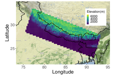
(a)

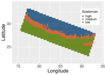
(b)

Figure 4: Left: topographic map of the study region; right: elevation subdomains.

To model extremal dependence, we must first transform the monthly maxima data onto the unit Fréchet scale. To account for spatial nonstationarity in the margins, we require estimates of location-dependent GEV parameters as in (1). To accommodate temporal nonstationarity, e.g., seasonality, in the time series, harmonic terms are imposed in the modeling of the location $\mu(\bm{s})$ and scale $\varsigma(\bm{s})$. The shape parameter $\xi(\bm{s})$ is fixed with respect to time for each location. The marginal model for monthly maxima $Y_{t}(\bm{s}_{i})$ at site $\bm{s}_{i}\in\mathcal{S}$ and month $t$ is

$$Y_{t}(\bm{s}_{i})\overset{\mathrm{ind}}{\sim}\operatorname{GEV}\{\mu_{t}(\bm{s}_{i}),\varsigma_{t}(\bm{s}_{i}),\xi(\bm{s}_{i})\},$$

for all $i=1,\ldots,D$ and $t=1,\ldots,T$, with

$$\mu_{t}(\bm{s}_{i})=\mu_{0}(\bm{s}_{i})+\mu_{1}(\bm{s}_{i})\sin(2\pi t_{month}/12)+\mu_{2}(\bm{s}_{i})\cos(2\pi t_{month}/12),\text{ and}$$ (13)

$$\log[\varsigma_{t}(\bm{s}_{i})]=\varsigma_{0}(\bm{s}_{i})+\varsigma_{1}(\bm{s}_{i})\sin(2\pi t_{month}/12)+\varsigma_{2}(\bm{s}_{i})\cos(2\pi t_{month}/12),$$

where $t_{month}$ is the index of the corresponding month of each observation, and $\mu_{0}(\bm{s})$, $\mu_{1}(\bm{s})$, and $\mu_{2}(\bm{s})$ ($\varsigma_{0}(\bm{s})$, $\varsigma_{1}(\bm{s})$, and $\varsigma_{2}(\bm{s})$) are coefficients for covariates of the location (scale) structure. Bayesian inference for spatially-varying marginal parameters may be performed flexibly and quickly using the Max-and-Smooth method, introduced by Hrafnkelsson et al. (2021), Jóhannesson et al. (2022), and Hazra et al. (2021), where unknown GEV parameters are transformed using specific link functions and then assumed to follow a multivariate Gaussian distribution with fixed and random effects at a latent level. Approximate Bayesian inference is performed using the stochastic partial differential equations approach and MCMC methods (see references for full details). Using the posterior mean of each marginal parameter, we transform the original data onto the unit Fréchet scale. We draw the quantile-quantile (QQ) plot for transformed data and conduct a hypothesis testing based on Kolmogorov–Smirnov distance, whose results show that the marginal fit is satisfactory overall (see Section LABEL:Supp:MASDiag in the supplementary materials for details).

We then fit five BR max-stable models to the standardized data: a stationary model (model S), and our proposed nonstationary model with a base and fully merged partition (Model B and M), using both $L_{1}$ and $L_{2}$ regularization; we compare the performance of all five models. The base partition (Figure 5) consists of 80 subregions and is generated using $k$-means clustering on standardized longitude and latitude coordinates. To evaluate model performance, a validation set ($15\%$) is randomly sampled from all observation sites. To tune the smoothness penalty $\bm{\lambda}$ and merge subregions, we split the remaining locations into 5 holdout folds, ensuring that there is at least one holdout site in each subregion for each fold. The initial descending grid for the $\bm{\lambda}$-tuning procedure is chosen to be $\bm{\Lambda}^{0}=(\infty,2^{5},2^{4},2^{3},2^{2},2^{1},2^{0},2^{-1},2^{-2},0)$; see Algorithm 1 in Section 3.2. We compute the PL on the validation set, the holdout PPL averaged over folds, and the CLIC and CBIC metrics for the remaining data excluding the validation set.

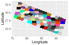
(a)

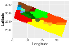
(b)

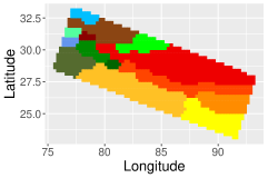
(c)

Figure 5: Left: base partition (80 subregions). Estimated merged partitions with $L_{1}$ (centre) and $L_{2}$ (right) regularization.

Table 3: Model performance metrics ($\times 10^{3}$). The number of parameters for each model is provided in brackets. The best value in each row is in bold.

	Sta.(2)	$L_{1}$		$L_{2}$
		Base (160)	Merged (28)	Base (160)	Merged (28)
PL	$-18066$	$-17975$	-17960	$-17966$	$-17963$
PPL	–	$-10400$	$-10395$	$-10394$	-10391
CLIC	$1180692$	$1171161$	$1169603$	$1170135$	1169505
CBIC	$1181132$	$1173024$	1170104	$1171403$	$1170314$

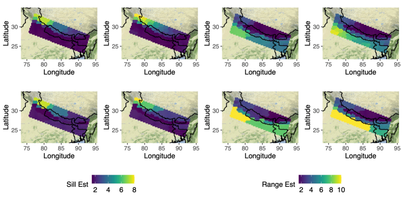
(a)

Figure 6: Estimated sill (left block) and range (right block) parameters with base partition (top row) and merged partition (bottom row). Each 2-by-2 block displays Model B (top) and M (bottom) with $L_{1}$ (left column) and $L_{2}$ (right column) regularization.

Table 3 shows that all nonstationary models provide a better fit than the stationary one, as we observe improvement in all goodness-of-fit metrics; we further observe that Model M outperforms Model B, regardless of the regularization used. For Model M, we find that $L_{2}$ regularization performs slightly better, when performing the comparison using PPL or CLIC, but the opposite holds in terms of PL and CBIC. Figure 5 shows the final estimated partitions for both regularization schemes, while estimates of the sill and range parameters are given in Figure 6. The partitions roughly identify the plain and mountainous areas shown in Figure 4, suggesting that there is significantly different extremal dependence behaviour in these areas. All nonstationary models provide larger sill estimates and smaller range estimates in mountainous regions compared to the plains, suggesting that extremal dependence in these areas decays faster with distance; the converse holds for the plains.

As a further model diagnostic, we compare the theoretical extremal coefficients, defined in (6) from the fitted models with their empirical counterparts; empirical estimates $\widetilde{\nu}(\bm{s}_{i},\bm{s}_{j})$ are obtained using the $F$-madogram (see Section 2.1). As the resulting empirical extremal coefficient $\widetilde{\theta}(\bm{s}_{i},\bm{s}_{j})$ does not necessarily lie in the interval $[1,2]$, we truncate estimates outside of this interval. Computation was conducted using the R package SpatialExtremes (Ribatet, 2020). To assess model fits, we partition the domain into 3 subdomains according to low, medium, and high elevation (see Figure 4), and compute pairwise extremal coefficients for all pairs of sites within each subdomain. Figure LABEL:pic:nepal_extDep_nonsta in the supplementary materials displays the theoretical extremal coefficients for the different model fits against their empirical counterparts. We further compute the mean absolute difference (MAD) between the theoretical and empirical extremal coefficients for all pairs of sites in the whole domain and in each elevation subdomain, and report the results in Table 4.

From Figure LABEL:pic:nepal_extDep_nonsta, we observe that the stationary model fails completely at identifying the varied extremal dependence behavior within each subdomain, while the nonstationary models, regardless of the partition and penalty used, provide a much better description of different extremal dependence behaviour. While the theoretical extremal coefficients for the nonstationary models may appear to slightly underestimate the extremal dependence (comparing to the empirical ones), it is important to note that this apparent lack of fit may be due to the high variability of the empirical estimates. We here have 192 independent monthly maxima replicates, and hence the empirical extremal coefficients may not be estimated well, especially in weak-dependence settings when $\theta(\bm{s}_{i},\bm{s}_{j})\approx 2$. Another reason might be that the exponential variogram we used has limited flexibility for capturing long-range independence. Model M better describes nonstationary extremal dependence behaviours overall, especially in low-elevation subdomain, which is confirmed by the MADs (see Table 4). Nonstationary models significantly outperform the stationary one in the low-elevation and middle-elevation subdomains in terms of MAD, with Model M slightly outperforming Model B. In the middle-elevation subdomain, models S and B are comparable, but Model M provides the smallest MAD. In the high-elevation subdomain, model S gives a slightly better fit than the nonstationary models, which is reasonable because nonstationary models give more realistic (larger) fitted values with increasing uncertainty in the high-elevation subdomain. However, Model M again outperforms Model B. Finally, the total MAD between theoretical and empirical extremal coefficients for the whole domain is smaller for the nonstationary models, with Model M outperforming Model B. Therefore, we conclude that the nonstationary models provide better estimates of the extremal dependence structure of Nepal temperatures, and our proposed merging procedure can further improve the fit, with $L_{2}$ regularization generally outperforming $L_{1}$ regularization.

Table 4: Mean absolute differences for pairwise extremal coefficients, with pairs in the whole domain (“Total”) or stratified by elevation subdomain (“Low”, “Medium”, and “High”).

	Sta.	$L_{1}$		$L_{2}$
		Model B	Model M	Model B	Model M
Total	0.203	0.156	0.150	0.152	0.149
Low	0.250	0.109	0.108	0.103	0.095
Medium	0.248	0.169	0.164	0.168	0.163
High	0.119	0.253	0.213	0.245	0.216

6 Concluding Remarks

In this paper, we propose a flexible, yet relatively parsimonious model for nonstationary extremal dependence using the Brown–Resnick max-stable process, and we develop a new computationally-efficient method to simultaneously estimate unknown parameters, identify stationary subregions, and reduce the number of model parameters. More precisely, our model is created by constructing a nonstationary variogram and partitioning the study domain into locally-stationary subregions. We further propose practical strategies for merging subregions, to create a parsimonious model in a data-driven way, without expert knowledge. Inference is performed using a pairwise likelihood to mitigate computational expense, and its statistical efficiency is investigated. In both our simulation study and application, we show that our model provides good fits to data, and better captures nonstationarity in extremal dependence, significantly improving on models previously seen in the literature.

We find in our simulation study that even when the base partition is misspecified, we still observe improved model fits over stationary models, but even better fits are observable with a well-specified base partition. Choosing the base partition for our model can be problematic, as subregions in the base partition may overlap with the boundaries in the true partition (if one exists). To mitigate this, we could divide the domain into finer subregions, but this may lead to unreliable parameter estimation. Another possible approach could be to allow subregions to split at each step as well as merge.

Our nonstationary Brown–Resnick max-stable process model uses an exponential variogram, which is bounded above as the distance between locations $\bm{s}_{i}$ and $\bm{s}_{j}$ increases, and hence our model can only capture asymptotic dependence; it cannot capture situations where two sufficiently distant sites are independent. In a relatively small domain of study, asymptotic dependence everywhere may be a reasonable assumption to make, but this may not be the case for large, or topographically complex regions; creating valid unbounded nonstationary variograms would be required to make our methodology more flexible. Moreover, even with an unbounded variogram, the model would not be able to capture forms of asymptotic independence other than perfect independence, as it uses max-stable processes. However, asymptotic independence can be accommodated by adapting our methodology to inverted MSPs (Wadsworth and Tawn, 2012), or other types of asymptotic independence models, such as certain types of Gaussian location-scale mixtures (Opitz, 2016; Huser et al., 2017; Hazra et al., 2022; Zhang et al., 2022), which are more flexible to capture sub-asymptotic extremal dependence (Huser and Wadsworth, 2022).

Further work includes an extension to incorporate local anisotropy and adapting our methodology to other max-stable processes, e.g., extremal-$t$; the former can be easily accommodated by parameterizing the matrix $\Omega(\bm{s})$ in (10). Our approach could also be extended to other spatial extreme models, such as Pareto processes (de Fondeville and Davison, 2018) or the spatial conditional extremes model (Wadsworth and Tawn, 2022).

SUPPLEMENTARY MATERIAL

PDF Supplement:

This supplement contains further details on the algorithm; additional simulation results; and further results for the data application (marginal and dependence goodness-of-fit diagnostics) (PDF file)

R Code:

This supplement contains the implementation of our proposed method in R, along with the real Nepal temperature dataset, and a small simulation example (zip file)

References

- Bevilacqua et al. (2012) Bevilacqua, M., C. Gaetan, J. Mateu, and E. Porcu (2012). Estimating space and space-time covariance functions for large data sets: A weighted composite likelihood approach. Journal of the American Statistical Association 107(497), 268–280.
- Blanchet and Davison (2011) Blanchet, J. and A. C. Davison (2011). Spatial modeling of extreme snow depth. The Annals of Applied Statistics 5, 1699–1725.
- Brown and Resnick (1977) Brown, B. M. and S. I. Resnick (1977). Extreme values of independent stochastic processes. Journal of Applied Probability 14(4), 732–739.
- Castro-Camilo and Huser (2020) Castro-Camilo, D. and R. Huser (2020). Local likelihood estimation of complex tail dependence structures, applied to us precipitation extremes. Journal of the American Statistical Association 115(531), 1037–1054.
- Castruccio et al. (2016) Castruccio, S., R. Huser, and M. G. Genton (2016). High-order composite likelihood inference for max-stable distributions and processes. Journal of Computational and Graphical Statistics 25(4), 1212–1229.
- Chevalier et al. (2021) Chevalier, C., O. Martius, and D. Ginsbourger (2021). Modeling nonstationary extreme dependence with stationary max-stable processes and multidimensional scaling. Journal of Computational and Graphical Statistics 30(3), 745–755.
- Cooley et al. (2006) Cooley, D., P. Naveau, and P. Poncet (2006). Variograms for spatial max-stable random fields. In Dependence in Probability and Statistics, pp. 373–390. Springer.
- Cooley et al. (2007) Cooley, D., D. Nychka, and P. Naveau (2007). Bayesian spatial modeling of extreme precipitation return levels. Journal of the American Statistical Association 102(479), 824–840.
- de Fondeville and Davison (2018) de Fondeville, R. and A. C. Davison (2018). High-dimensional peaks-over-threshold inference. Biometrika 105(3), 575–592.
- de Haan (1984) de Haan, L. (1984). A spectral representation for max-stable processes. The Annals of Probability 12, 1194–1204.
- de Haan and Ferreira (2007) de Haan, L. and A. Ferreira (2007). Extreme Value Theory: An Introduction. Springer Science & Business Media.
- Fuentes (2001) Fuentes, M. (2001). A high frequency kriging approach for non-stationary environmental processes. Environmetrics 12(5), 469–483.
- Fuentes (2002) Fuentes, M. (2002). Interpolation of nonstationary air pollution processes: A spatial spectral approach. Statistical Modelling 2(4), 281–298.
- Gerber and Nychka (2021) Gerber, F. and D. Nychka (2021). Fast covariance parameter estimation of spatial Gaussian process models using neural networks. Stat 10(1), e382.
- Hazra et al. (2022) Hazra, A., R. Huser, and D. Bolin (2022). Realistic and fast modeling of spatial extremes over large geographical domains. arXiv preprint 2112.10248.
- Hazra et al. (2021) Hazra, A., R. Huser, and Á. V. Jóhannesson (2021). Bayesian latent Gaussian models for high-dimensional spatial extremes. In B. Hrafnkelsson (Ed.), Statistical Modeling Using Bayesian Latent Gaussian Models. Springer.
- Hrafnkelsson et al. (2021) Hrafnkelsson, B., S. Siegert, R. Huser, H. Bakka, and Á. V. Jóhannesson (2021). Max-and-Smooth: A two-step approach for approximate Bayesian inference in latent Gaussian models. Bayesian Analysis 16(2), 611–638.
- Huser (2013) Huser, R. (2013). Statistical modeling and inference for spatio-temporal extremes. Technical report, École Polytechnique Fédérale de Lausanne (EPFL).
- Huser and Davison (2013) Huser, R. and A. C. Davison (2013). Composite likelihood estimation for the Brown–Resnick process. Biometrika 100(2), 511–518.
- Huser and Davison (2014) Huser, R. and A. C. Davison (2014). Space-time modelling of extreme events. Journal of the Royal Statistical Society: Series B 76(2), 439–461.
- Huser et al. (2019) Huser, R., C. Dombry, M. Ribatet, and M. G. Genton (2019). Full likelihood inference for max-stable data. Stat 8(1), e218.
- Huser and Genton (2016) Huser, R. and M. G. Genton (2016). Non-stationary dependence structures for spatial extremes. Journal of Agricultural, Biological, and Environmental Statistics 21, 470–491.
- Huser et al. (2017) Huser, R., T. Opitz, and E. Thibaud (2017). Bridging asymptotic independence and dependence in spatial extremes using Gaussian scale mixtures. Spatial Statistics 21, 166–186.
- Huser et al. (2022) Huser, R., M. L. Stein, and P. Zhong (2022). Vecchia likelihood approximation for accurate and fast inference in intractable spatial extremes models. arXiv preprint 2203.05626.
- Huser and Wadsworth (2022) Huser, R. and J. L. Wadsworth (2022). Advances in statistical modeling of spatial extremes. Wiley Interdisciplinary Reviews: Computational Statistics 14(1), e1537.
- Jóhannesson et al. (2022) Jóhannesson, Á. V., S. Siegert, R. Huser, H. Bakka, and B. Hrafnkelsson (2022). Approximate bayesian inference for analysis of spatiotemporal flood frequency data. The Annals of Applied Statistics 16(2), 905–935.
- Kabluchko et al. (2009) Kabluchko, Z., M. Schlather, and L. de Haan (2009). Stationary max-stable fields associated to negative definite functions. The Annals of Probability 37(5), 2042–2065.
- Lenzi et al. (2021) Lenzi, A., J. Bessac, J. Rudi, and M. L. Stein (2021). Neural networks for parameter estimation in intractable models. arXiv preprint 2107.14346.
- Muyskens et al. (2022) Muyskens, A., J. Guinness, and M. Fuentes (2022). Partition-based nonstationary covariance estimation using the stochastic score approximation. Journal of Computational and Graphical Statistics. To appear.
- Ng and Joe (2014) Ng, C. T. and H. Joe (2014). Model comparison with composite likelihood information criteria. Bernoulli 20(4), 1738–1764.
- Opitz (2013) Opitz, T. (2013). Extremal t processes: Elliptical domain of attraction and a spectral representation. Journal of Multivariate Analysis 122, 409–413.
- Opitz (2016) Opitz, T. (2016). Modeling asymptotically independent spatial extremes based on Laplace random fields. Spatial Statistics 16, 1–18.
- Paciorek and Schervish (2006) Paciorek, C. J. and M. J. Schervish (2006). Spatial modelling using a new class of nonstationary covariance functions. Environmetrics 17(5), 483–506.
- Padoan et al. (2010) Padoan, S. A., M. Ribatet, and S. A. Sisson (2010). Likelihood-based inference for max-stable processes. Journal of the American Statistical Association 105(489), 263–277.
- Parker et al. (2016) Parker, R. J., B. J. Reich, and J. Eidsvik (2016). A fused LASSO approach to nonstationary spatial covariance estimation. Journal of Agricultural, Biological, and Environmental Statistics 21(3), 569–587.
- Reich and Shaby (2012) Reich, B. J. and B. A. Shaby (2012). A hierarchical max-stable spatial model for extreme precipitation. The Annals of Applied Statistics 6(4), 1430.
- Ribatet (2020) Ribatet, M. (2020). SpatialExtremes: Modelling Spatial Extremes. R package version 2.0-8. https://CRAN.R-project.org/package=SpatialExtremes.
- Richards and Wadsworth (2021) Richards, J. and J. L. Wadsworth (2021). Spatial deformation for nonstationary extremal dependence. Environmetrics 32(5), e2671.
- Rodell et al. (2004) Rodell, M., P. Houser, U. Jambor, J. Gottschalck, K. Mitchell, C.-J. Meng, K. Arsenault, B. Cosgrove, J. Radakovich, M. Bosilovich, et al. (2004). The global land data assimilation system. Bulletin of the American Meteorological society 85(3), 381–394.
- Sainsbury-Dale et al. (2022) Sainsbury-Dale, M., A. Zammit-Mangion, and R. Huser (2022). Fast optimal estimation with intractable models using permutation-invariant neural networks. arXiv preprint 2208.12942.
- Sampson and Guttorp (1992) Sampson, P. D. and P. Guttorp (1992). Nonparametric estimation of nonstationary spatial covariance structure. Journal of the American Statistical Association 87(417), 108–119.
- Sass et al. (2021) Sass, D., B. Li, and B. J. Reich (2021). Flexible and fast spatial return level estimation via a spatially fused penalty. Journal of Computational and Graphical Statistics 30, 1124–1142.
- Schlather (2002) Schlather, M. (2002). Models for stationary max-stable random fields. Extremes 5(1), 33–44.
- Schlather and Tawn (2003) Schlather, M. and J. A. Tawn (2003). A dependence measure for multivariate and spatial extreme values: Properties and inference. Biometrika 90(1), 139–156.
- Smith (1990) Smith, R. L. (1990). Max-stable processes and spatial extremes. Unpublished manuscript. https://www.rls.sites.oasis.unc.edu/postscript/rs/spatex.pdf.
- Stein et al. (2004) Stein, M. L., Z. Chi, and L. J. Welty (2004). Approximating likelihoods for large spatial data sets. Journal of the Royal Statistical Society: Series B 66(2), 275–296.
- Vecchia (1988) Vecchia, A. V. (1988). Estimation and model identification for continuous spatial processes. Journal of the Royal Statistical Society: Series B 50(2), 297–312.
- Wadsworth and Tawn (2022) Wadsworth, J. and J. Tawn (2022). Higher-dimensional spatial extremes via single-site conditioning. Spatial Statistics 51, 100677.
- Wadsworth and Tawn (2012) Wadsworth, J. L. and J. A. Tawn (2012). Dependence modelling for spatial extremes. Biometrika 99(2), 253–272.
- Zhang et al. (2022) Zhang, Z., R. Huser, T. Opitz, and J. Wadsworth (2022). Modeling spatial extremes using normal mean-variance mixtures. Extremes 25(2), 175–197.