C-Mixup: Improving Generalization in Regression

Abstract

Improving the generalization of deep networks is an important open challenge, particularly in domains without plentiful data. The mixup algorithm improves generalization by linearly interpolating a pair of examples and their corresponding labels. These interpolated examples augment the original training set. Mixup has shown promising results in various classification tasks, but systematic analysis of mixup in regression remains underexplored. Using mixup directly on regression labels can result in arbitrarily incorrect labels. In this paper, we propose a simple yet powerful algorithm, C-Mixup, to improve generalization on regression tasks. In contrast with vanilla mixup, which picks training examples for mixing with uniform probability, C-Mixup adjusts the sampling probability based on the similarity of the labels. Our theoretical analysis confirms that C-Mixup with label similarity obtains a smaller mean square error in supervised regression and meta-regression than vanilla mixup and using feature similarity. Another benefit of C-Mixup is that it can improve out-of-distribution robustness, where the test distribution is different from the training distribution. By selectively interpolating examples with similar labels, it mitigates the effects of domain-associated information and yields domain-invariant representations. We evaluate C-Mixup on eleven datasets, ranging from tabular to video data. Compared to the best prior approach, C-Mixup achieves 6.56%, 4.76%, 5.82% improvements in in-distribution generalization, task generalization, and out-of-distribution robustness, respectively. Code is released at https://github.com/huaxiuyao/C-Mixup.

1 Introduction

Deep learning practitioners commonly face the challenge of overfitting. To improve generalization, prior works have proposed a number of techniques, including data augmentation [3, 10, 12, 81, 82] and explicit regularization [15, 38, 60]. Representatively, mixup [82, 83] densifies the data distribution and implicitly regularizes the model by linearly interpolating the features of randomly sampled pairs of examples and applying the same interpolation on the corresponding labels. Despite mixup having demonstrated promising results in improving generalization in classification problems, it has rarely been studied in the context of regression with continuous labels, on which we focus in this paper.

In contrast to classification, which formalizes the label as a one-hot vector, the goal of regression is to predict a continuous label from each input. Directly applying mixup to input features and labels in regression tasks may yield arbitrarily incorrect labels. For example, as shown in Figure 1(a), ShapeNet1D pose prediction [18] aims to predict the current orientation of the object relative to its canonical orientation. We randomly select three mixing pairs and show the mixed images and labels in Figure 1(b), where only pair 1 exhibits reasonable mixing results. We thus see that sampling mixing pairs uniformly from the dataset introduces a number of noisy pairs.

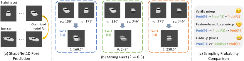
Figure 1: Illustration of C-Mixup on ShapeNet1D pose prediction. $\lambda$ represents the interpolation ratio. (a) ShapeNet1D pose prediction task, aiming to predict the current orientation of the object relative to its canonical orientation. (b) Three mixing pairs are randomly picked, where the interpolated images are visualized and $\tilde{y}$ represents interpolated labels. (c) Illustration of a rough comparison of sampling probabilities among three mixing pairs in (b). The Euclidean distance measures input feature distance and the corresponding results between examples in pairs 1, 2, 3 are $1.51\times 10^{5}$, $1.82\times 10^{5}$, $1.50\times 10^{5}$, respectively. Hence, pairs 1 and 3 have similar results, leading to similar sampling probabilities. C-Mixup is able to assign higher sampling probability for more reasonable mixing pairs.

In this paper, we aim to adjust the sampling probability of mixing pairs according to the similarity of examples, resulting in a simple training technique named C-Mixup. Specifically, we employ a Gaussian kernel to calculate the sampling probability of drawing another example for mixing, where closer examples are more likely to be sampled. Here, the core question is: how to measure the similarity between two examples? The most straightforward solution is to compute input feature similarity. Yet, using input similarity has two major downsides when dealing with high-dimensional data such as images or time-series: substantial computational costs and lack of good distance metrics. Specifically, it takes considerable time to compute pairwise similarities across all samples, and directly applying classical distance metrics (e.g., Euclidean distance, cosine distance) does not reflect the high-level relation between input features. In the ShapeNet1D rotation prediction example (Figure 1(a)), pair 1 and 3 have close input similarities, while only pair 1 can be reasonably interpolated.

To overcome these drawbacks, C-Mixup instead uses label similarity, which is typically much faster to compute since the label space is usually low dimensional. In addition to the computational advantages, C-Mixup benefits three kinds of regression problems. First, it empirically improves in-distribution generalization in supervised regression compared to using vanilla mixup or using feature similarity. Second, we extend C-Mixup to gradient-based meta-learning by incorporating it into MetaMix, a mixup-based task augmentation method [74]. Compared to vanilla MetaMix, C-Mixup empirically improves task generalization. Third, C-Mixup is well-suited for improving out-of-distribution robustness without domain information, particularly to covariate shift (see the corresponding example in Appendix A.1). By performing mixup on examples with close continuous labels, examples with different domains are mixed. In this way, C-Mixup encourages the model to rely on domain-invariant features to make prediction and ignore unrelated or spurious correlations, making the model more robust to covariate shift.

The primary contribution of this paper is C-Mixup, a simple and scalable algorithm for improving generalization in regression problems. In linear or monotonic non-linear models, our theoretical analysis shows that C-Mixup improves generalization in multiple settings compared to vanilla mixup or compared to using feature similarities. Moreover, our experiments thoroughly evaluate C-Mixup on eleven datasets, including many large-scale real-world applications like drug-target interaction prediction [28], ejection fraction estimation with echocardiogram videos [50], poverty estimation with satellite imagery [78]. Compared to the best prior method, the results demonstrate the promise of C-Mixup with 6.56%, 4.76%, 5.82% improvements in in-distribution generalization, task generalization, and out-of-distribution robustness, respectively.

2 Preliminaries

In this section, we define notation and describe the background of ERM and mixup in the supervised learning setting, and MetaMix in the meta-learning setting for task generalization.

ERM. Assume a machine learning model $f$ with parameter space $\Theta$. In this paper, we consider the setting where one predicts the continuous label $y\in\mathcal{Y}$ according to the input feature $x\in\mathcal{X}$. Given a loss function $\ell$, we train a model $f_{\theta}$ under the empirical training distribution $P^{tr}$ with the following objective, and get the optimized parameter $\theta^{*}\in\Theta$:

$$\small\theta^{*}\leftarrow\arg\min_{\theta\in\Theta}\mathbb{E}_{(x,y)\sim P^{tr}}[\ell(f_{\theta}(x),y)].$$ (1)

Typically, we expect the model to perform well on unseen examples drawn from the test distribution $P^{ts}$. We are interested in both in-distribution ($P^{tr}=P^{ts}$) and out-of-distribution ($P^{tr}\neq P^{ts}$) settings.

Mixup. The mixup algorithm samples a pair of instances $(x_{i},y_{i})$ and $(x_{j},y_{j})$, sampled uniformly at random from the training dataset, and generates new examples by performing linear interpolation on the input features and corresponding labels as:

$$\small\tilde{x}=\lambda\cdot x_{i}+(1-\lambda)\cdot x_{j},\;\tilde{y}=\lambda\cdot y_{i}+(1-\lambda)\cdot y_{j},$$ (2)

where the interpolation ratio $\lambda\in[0,1]$ is drawn from a Beta distribution, i.e., $\lambda\sim\mathrm{Beta}(\alpha,\alpha)$. The interpolated examples are then used to optimize the model as follows:

$$\small\theta^{*}\leftarrow\arg\min_{\theta\in\Theta}\mathbb{E}_{(x_{i},y_{i}),(x_{j},y_{j})\sim P^{tr}}[\ell(f_{\theta}(\tilde{x}),\tilde{y})].$$ (3)

Task Generalization and MetaMix. In this paper, we also investigate few-shot task generalization under the gradient-based meta-regression setting. Given a task distribution $p(\mathcal{T})$, we assume each task $\mathcal{T}_{m}$ is sampled from $p(\mathcal{T})$ and is associated with a dataset $\mathcal{D}_{m}$. A support set $\mathcal{D}_{m}^{s}=\{(X_{m}^{s},Y_{m}^{s})\}=\{(x_{m,i}^{s},y_{m,i}^{s})\}_{i=1}^{N^{s}}$ and a query set $\mathcal{D}_{m}^{q}=\{(X_{m}^{s},Y_{m}^{s})\}=\{(x_{m,j}^{q},y_{m,j}^{q})\}_{i=1}^{N^{q}}$ are sampled from $\mathcal{D}_{m}$. Representatively, in model-agnostic meta-learning (MAML) [14], given a predictive model $f$ with parameter $\theta$, it aims to learn an initialization $\theta^{*}$ from meta-training tasks $\{\mathcal{T}_{m}\}_{m=1}^{|M|}$. Specifically, at the meta-training phase, MAML obtained the task-specific parameter $\phi_{m}$ for each task $\mathcal{T}_{m}$ by performing a few gradient steps starting from $\theta$. Then, the corresponding query set $\mathcal{D}_{m}^{q}$ is used to evaluate the performance of the task-specific model and optimize the model initialization as:

$$\small\theta^{*}:=\arg\min_{\theta}\frac{1}{|M|}\sum_{i=1}^{|M|}\mathcal{L}(f_{\phi_{m}};\mathcal{D}_{m}^{q}),\;where\;\;\phi_{m}=\theta-\alpha\nabla_{\theta}\mathcal{L}(f_{\theta};\mathcal{D}_{m}^{s})$$ (4)

At the meta-testing phase, for each meta-testing task $\mathcal{T}_{t}$, MAML fine-tunes the learned initialization $\theta^{*}$ on the support set $\mathcal{D}_{t}^{s}$ and evaluates the performance on the corresponding query set $\mathcal{D}_{t}^{q}$.

To improve task generalization, MetaMix [74] adapts mixup (Eqn. (3)) to meta-learning, which linearly interpolates the support set and query set and uses the interpolated set to replace the original query set $\mathcal{D}^{q}_{m}$ in Eqn. (4). Specifically, the interpolated query set is formulated as:

$$\small\tilde{X}_{m}^{q}=\lambda X_{m}^{s}+(1-\lambda)X_{m}^{q},\;\tilde{Y}_{m}^{q}=\lambda Y_{m}^{s}+(1-\lambda)Y_{m}^{q},$$ (5)

where $\lambda\sim\mathrm{Beta}(\alpha,\alpha)$.

3 Mixup for Regression (C-Mixup)

For continuous labels, the example in Figure 1(b) illustrates that applying vanilla mixup to the entire distribution is likely to produce arbitrary labels. To resolve this issue, C-Mixup proposes to sample closer pairs of examples with higher probability. Specifically, given an example $(x_{i},y_{i})$, C-Mixup introduces a symmetric Gaussian kernel to calculate the sampling probability $P((x_{j},y_{j})|(x_{i},y_{i}))$ for another $(x_{j},y_{j})$ example to be mixed as follows:

$$\small P((x_{j},y_{j})|(x_{i},y_{i}))\propto\exp\left(-\frac{d(i,j)}{2\sigma^{2}}\right)$$ (6)

where $d(i,j)$ represents the distance between the examples $(x_{i},y_{i})$ and $(x_{j},y_{j})$, and $\sigma$ describes the bandwidth. For the example $(x_{i},y_{i})$, the set $\{P((x_{j},y_{j})|(x_{i},y_{i}))|\forall j\}$ is then normalized to a probability mass function that sums to one.

Algorithm 1 Training with C-Mixup

0:  Learning rates $\eta$; Shape parameter $\alpha$

0:  Training data $\mathcal{D}:=\{(x_{i},y_{i})\}_{i=1}^{N}$

1:  Randomly initialize model parameters $\theta$

2:  Calculate pairwise distance matrix $P$ via Eqn. (6)

3:  while not converge do

4:     Sample a batch of examples $\mathcal{B}\sim\mathcal{D}$

5:     for each example $(x_{i},y_{i})\in\mathcal{B}$ do

6:        Sample ($x_{j}$, $y_{j}$) from $P(\cdot\mid(x_{i},y_{i}))$ and $\lambda$ from $\mathrm{Beta}(\alpha,\alpha)$

7:        Interpolate ($x_{i}$, $y_{i}$), ($x_{j}$, $y_{j}$) to get ($\tilde{x},\tilde{y}$) according to Eqn. (2)

8:     Use interpolated examples to update the model via Eqn. (3)

One natural way to compute the distance is using the input feature $x$, i.e., $d(i,j)=d(x_{i},x_{j})$. However, when dealing with the high-dimensional data such as images or videos, we lack good distance metrics to capture structured feature information and the distances can be easily influenced by feature noise. Additionally, computing feature distances for high-dimensional data is time-consuming. Instead, C-Mixup leverages the labels with $d(i,j)=d(y_{i},y_{j})=\|y_{i}-y_{j}\|_{2}^{2}$, where $y_{i}$ and $y_{j}$ are vectors with continuous values. The dimension of label is typically much smaller than that of the input feature, therefore reducing computational costs (see more discussions about compuatational efficiency in Appendix A.3). The overall algorithm of C-Mixup is described in Alg. 1 and we detail the difference between C-Mixup and mixup in Appendix A.4. According to Alg. 1, C-Mixup assigns higher probabilities to example pairs with closer continuous labels. In addition to its computational benefits, C-Mixup improves generalization on three distinct kinds of regression problems – in-distribution generalization, task generalization, and out-of-distribution robustness, which is theoretically and empirically justified in the following sections.

4 Theoretical Analysis

In this section, we theoretically explain how C-Mixup benefits in-distribution generalization, task generalization, and out-of-distribution robustness.

4.1 C-Mixup for Improving In-Distribution Generalization

In this section, we show that C-Mixup provably improves in-distribution generalization when the features are observed with noise, and the response depends on a small fraction of the features in a monotonic way. Specifically, we consider the following single index model with measurement error,

$$\small y=g(\theta^{\top}z)+\epsilon,$$ (7)

where $\theta\in\mathbb{R}^{p}$ and $\epsilon$ is a sub-Gaussian random variable and $g$ is a monotonic transformation. Since images are often inaccurately observed in practice, we assume the feature $z$ is observed or measured with noise, and denote the observed value by $x$: $x=z+\xi$ with $\xi$ being a random vector with mean 0 and covariance matrix $\sigma_{\xi}^{2}I$. We assume $g$ to be monotonic to model the nearly one-to-one correspondence between causal features (e.g., the car pose in Figure 1(a)) and labels (rotation) in the in-distribution setting. The out-of-distribution setting will be discussed in Section 4.3. We would like to also comment that the single index model has been commonly used in econometrics, statistics, and deep learning theory [19, 27, 47, 53, 73].

Suppose we have $\{(x_{i},y_{i})\}_{i=1}^{N}$ i.i.d. drawn from the above model. We first follow the single index model literature (e.g. [73]) and estimate $\theta$ by minimizing the square error $\sum_{i=1}^{n}(\tilde{y}_{i}-\tilde{x}_{i}^{\top}\theta)^{2}$, where the $(\tilde{x}_{i},\tilde{y}_{i})^{\prime}s$ are the augmented data by either vanilla mixup, mixup with input feature similarity, and C-Mixup. We denote the solution by $\theta^{*}_{mixup}$, $\theta^{*}_{feat}$, and $\theta^{*}_{C-Mixup}$ respectively. Given an estimate $\theta^{*}$, we estimate $g$ by $\hat{g}$ via the standard nonparametric kernel estimator [64] (we specify this in detail in Appendix B.1 for completeness) using the augmented data. We consider the mean square error metric as $\mathrm{MSE}(\theta)=\mathbb{E}[(y-\hat{g}(\theta^{\top}x))^{2}]$, and then have the following theorem (proof: Appendix B.1):

Theorem 1.

Suppose $\theta\in\mathbb{R}^{p}$ is sparse with sparsity $s=o(\min\{p,\sigma_{\xi}^{2}\})$, $p=o(N)$ and $g$ is smooth with $c_{0}<g^{\prime}<c_{1}$, $c_{2}<g^{\prime\prime}<c_{3}$ for some universal constants $c_{0},c_{1},c_{2},c_{3}>0$. There exists a distribution on $x$ with a kernel function, such that when the sample size $N$ is sufficiently large, with probability $1-o(1)$,

$$\small\mathrm{MSE}(\theta^{*}_{C-Mixup})<\min(\mathrm{MSE}(\theta^{*}_{feat}),\mathrm{MSE}(\theta^{*}_{mixup})).$$ (8)

The high-level intuition of why C-Mixup helps is that the vanilla mixup imposes linearity regularization on the relationship between the feature and response. When the relationship is strongly nonlinear and one-to-one, such a regularization hurts the generalization, but could be mitigated by C-Mixup.

4.2 C-Mixup for Improving Task Generalization

The second benefit of C-Mixup is improving task generalization in meta-learning when the data from each task follows the model discussed in the last section. Concretely, we apply C-Mixup to MetaMix [74]. For each query example, the support example with a more similar label will have a higher probability of being mixed. The algorithm of C-Mixup on MetaMix is summarized in Appendix A.2.

Similar to in-distribution generalization analysis, we consider the following data generative model: for the $m$-th task ($m\in[M]$), we have $(x^{(m)},y^{(m)})\sim\mathcal{T}_{m}$ with

$$\small y^{(m)}=g_{m}(\theta^{\top}z^{(m)})+\epsilon\quad\text{ and }\quad x^{(m)}=z^{(m)}+\epsilon^{(m)}.$$ (9)

Here, $\theta$ denotes the globally-shared representation, and $g_{m}$’s are the task-specific transformations. Note that, the formulation is close to [54] and wildly applied to theoretical analysis of meta-learning [74, 77]. Following similar spirit of [62] and last section, we obtain the estimation of $\theta$ by $\small\theta^{*}=\frac{1}{M}\sum_{m=1}^{M}(\mathbb{E}_{(\tilde{x}^{(m)},\tilde{y}^{(m)})\in\mathcal{\hat{D}}_{m}}[\tilde{y}^{(m)}-\theta^{\top}\tilde{x}^{(m)}]).$ Here, $\mathcal{\hat{D}}_{m}$ denotes the generic dataset augmented by different approaches, including the vanilla MetaMix, MetaMix with input feature similarity, and C-Mixup. We denote these approaches by $\theta^{*}_{MetaMix}$, $\theta^{*}_{Meta-feat}$, and $\theta^{*}_{Meta-C-Mixup}$ respectively. For a new task $\mathcal{T}_{t}$, we again use the standard nonparametric kernel estimator to estimate $g_{t}$ via the augmented target data. We then consider the following error metric $\small\mathrm{MSE}_{\mathrm{Target}}(\theta^{*})=\mathbb{E}_{(x,y)\sim\mathcal{T}_{t}}[(y-\hat{g}_{t}({\theta^{*}}^{\top}x))^{2}].$

Based on this metric, we get the following theorem to show the promise of C-Mixup in improving task generalization (see Appendix B.2 for detailed proof). Here, C-Mixup achieves smaller $\mathrm{MSE}_{\mathrm{Target}}$ compared to vanilla MetaMix and MetaMix with input feature similarity.

Theorem 2.

Let $N=\sum_{m=1}^{M}N_{m}$ and $N_{m}$ is the number of examples of $\mathcal{T}_{m}$. Suppose $\theta_{k}$ is sparse with sparsity $s=o(\min\{d,\sigma_{\xi}^{2}\})$, $p=o(N)$ and $g_{m}$’s are smooth with $0<g_{m}^{\prime}<c_{1}$, $c_{2}<g_{m}^{\prime\prime}<c_{3}$ for some universal constants $c_{1},c_{2},c_{3}>0$ and $m\in[M]\cup\{t\}$. There exists a distribution on $x$ with a kernel function, such that when the sample size $N$ is sufficiently large, with probability $1-o(1)$,

$$\small\mathrm{MSE}_{\mathrm{Target}}(\theta^{*}_{Meta-C-Mixup})<\min(\mathrm{MSE}_{\mathrm{Target}}(\theta^{*}_{Meta-feat}),\mathrm{MSE}_{\mathrm{Target}}(\theta^{*}_{MetaMix})).$$ (10)

4.3 C-Mixup for Improving Out-of-distribution Robustness

Finally, we show that C-Mixup improves OOD robustness in the covariate shift setting where some unrelated features vary across different domains. In this setting, we regard the entire data distribution consisting of $\mathcal{E}=\{1,\ldots,E\}$ domains, where each domain is associated with a data distribution $P_{e}$ for $e\in\mathcal{E}$. Given a set of training domains $\mathcal{E}^{tr}\subseteq\mathcal{E}$, we aim to make the trained model generalize well to an unseen test domain $\mathcal{E}^{ts}$ that is not necessarily in $\mathcal{E}^{tr}$. Here, we focus on covariate shift, i.e., the change of $P_{e}$ among domains is only caused by the change of marginal distribution $P_{e}(X)$, while the conditional distribution $P_{e}(Y|X)$ is fixed across different domains.

To overcome covariate shift, mixing examples with close labels without considering domain information can effectively average out domain-changeable correlations and make the predicted values rely on the invariant causal features. To further understand how C-Mixup improves the robustness to covariate shift, we provide the following theoretical analysis.

We assume the training data $(x_{i},y_{i})_{i=1}^{n}$ follows $x_{i}=(z_{i};a_{i})\in\mathbb{R}^{p_{1}+p_{2}}$ and $y_{i}=\theta^{\top}x_{i}+\epsilon_{i}$, where $z_{i}\in\mathbb{R}^{p_{1}}$ and $a_{i}\in\mathbb{R}^{p_{2}}$ are regarded as invariant and domain-changeable unrelated features, respectively, and the last $p_{2}$ coordinates of $\theta\in\mathbb{R}^{p_{1}+p_{2}}$ are 0. Now we consider the case where the training data consists of a pair of domains with almost identical invariant features and opposite domain-changeable features, i.e., $x_{i}=(z_{i},a_{i}),x_{i}^{\prime}=(z_{i}^{\prime},a_{i}^{\prime})$, where $z_{i}\sim\mathcal{N}_{p_{1}}(0,\sigma_{x}^{2}I_{p_{1}})$, $z_{i}^{\prime}=z_{i}+\epsilon_{i}^{\prime}$, $a_{i}\sim\mathcal{N}_{p_{2}}(0,\sigma_{a}^{2}I_{p_{2}})$, $a_{i}^{\prime}=-a_{i}+\epsilon_{i}^{\prime\prime}$. $\epsilon_{i},\epsilon_{i}^{\prime},\epsilon_{i}{{}^{\prime\prime}}$ are noise terms with mean 0 and sub-Gaussian norm bounded by $\sigma_{\epsilon}$. We use ridge estimator $\theta^{*}(k)=\mathop{\arg\min}_{\theta}({\sum_{i}\|{y_{i}-\theta^{\top}x_{i}}\|^{2}}+k\|\theta\|^{2})$ to reflect the implicit regularization effect of deep neural networks [48]. The covariant shift happens when the test domains have different $a_{i}$ distributions compared with training domains. We then have the following theorem to show that C-Mixup can improve robustness to covariant shift (see proof in Appendix B.3):

Theorem 3.

Supposed for some $\max(\exp(-n^{1-o(1)}),\exp(-\frac{p_{1}^{2}}{2n}))<\delta\ll 1$, we have variance constraints: $\sigma_{a}=c_{1}\sigma_{x}$ , $\sigma_{x}\geq c_{2}\max(\frac{n^{5/2}}{\|{\theta}\|\delta}\sigma_{\epsilon},\frac{\sqrt{p_{2}}\|{\theta}\|}{\sqrt{n}p_{1}})$ and $\sigma_{\epsilon}^{2}\leq\frac{c_{3}}{pn^{3/2}}$ . Then for any penalty k satisfies $c_{4}\sqrt{\frac{p_{2}}{p_{1}}}n^{1/4+o(1)}<k<c_{5}\min(\frac{\sigma_{x}}{\|{\theta}\|}\sqrt{p_{1}n^{1-o(1)}},n)$ and bandwidth h satisfies $0<h\leq c_{6}\frac{l}{\sqrt{\log(n^{2}/p_{1})}}$ in C-Mixup, when $n$ is sufficiently large, with probability at least $1-o(1)$, we have

$$\small\mathrm{MSE}(\theta^{*}_{C-Mixup})<\min(\mathrm{MSE}(\theta^{*}_{feat}),\mathrm{MSE}(\theta^{*}_{mixup})),$$ (11)

where $c_{1}\geq 1$, $c_{2}$, $c_{3}$, $c_{4}$, $c_{5}$, $c_{6}$ > 0 are universal constants, $l=\min_{i\neq j}\lvert y_{i}-y_{j}^{\prime}\rvert$ and $p_{1}\ll n<p_{1}^{2}$.

5 Experiments

In this section, we evaluate the performance of C-Mixup, aiming to answer the following questions: Q1: Compared to corresponding prior approaches, can C-Mixup improve the in-distribution, task generalization, and out-of-distribution robustness on regression? Q2: How does C-Mixup perform compared to using other distance metrics? Q3: Is C-Mixup sensitive to the choice of bandwidth $\sigma$ in the Gaussian kernel of Eqn. (6)? In our experiments, we apply cross-validation to tune all hyperparameters with grid search.

5.1 In-Distribution Generalization

Datasets. We use the following five datasets to evaluate the performance of in-distribution generalization (see Appendix C.1 for detailed data statistics). (1)&(2) Airfoil Self-Noise (Airfoil) and NO2 [35] are both are tabular datasets, where airfoil contains aerodynamic and acoustic test results of airfoil blade sections and NO2 aims to predict the mount of air pollution at a particular location. (3)&(4): Exchange-Rate, and Electricity [40] are two time-series datasets, where Exchange-Rate reports the collection of the daily exchange rates and Electricity is used to predict the hourly electricity consumption. (5) Echocardiogram Videos (Echo) [50] is a ejection fraction prediction dataset, which consists of a series of videos illustrating the heart from different aspects.

Comparisons and Experimental Setups. We compare C-Mixup with mixup and its variants (Manifold mixup [68], k-Mixup [20] and Local Mixup [5]) that can be easily to adapted to regression tasks. We also compare to MixRL, a recent reinforcement learning framework to select mixup pairs in regression. Note that, for k-Mixup, Local Mixup, MixRL, and C-Mixup, we apply them to both mixup and Manifold Mixup and report the best-performing combination.

For Airfoil and NO2, we employ a three-layer fully connected network as the backbone model. We use LST-Attn [40] for the Exchange-Rate and Electricity, and EchoNet-Dynamic [50] for predicting the ejection fraction. We use Root Mean Square Error (RMSE) and Mean Averaged Percentage Error (MAPE) as evaluation metrics. Detailed experimental setups are in Appendix C.2.

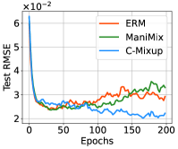
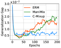
Figure 2: Overfitting Analysis on Exchange-Rate. C-Mixup achieves better test performance and smaller generalization gap.

Results. We report the results in Table 1 and have the following observations. First, vanilla mixup and manifold mixup are typically less performant than ERM when they are applied directly to regression tasks. These results support our hypothesis that random selection of example pairs for mixing may produce arbitrary inaccurate virtual labels. Second, while limiting the scope of interpolation (e.g., k-Mixup, Manifold k-Mixup, Local Mixup) helps to improve generalization in most cases, the performance of these approaches is inconsistent across different datasets. As an example, Local Mixup outperforms ERM in NO2 and Exchange-Rate, but fails to benefit results in Electricity. Third, even in more complicated datasets, such as Electricity and Echo, MixRL performs worse than Mixup and ERM, indicating that it is non-trivial to train a policy network that works well. Finally, C-Mixup consistently outperforms mixup and its variants, ERM, and MixRL, demonstrating its capability to improve in-distribution generalization on regression problems.

Analysis of Overfitting. In Figure 2, we visualize the test loss (RMSE) and the generalization gap between training loss and test loss of ERM, Manifold Mixup, and C-Mixup with respect to the training epoch for Exchange-Rate. More results are illustrated in Appendix C.3. Compared with ERM and C-Mixup, the better test performance and smaller generalization gap of C-Mixup further demonstrates its ability to improve in-distribution generalization and mitigate overfitting.

Table 1: Results for in-distribution generalization. We report the average RMSE and MAPE of three seeds. Full results with standard deviation are reported in Appendix C.4. The best results and second best results are bold and underlined, respectively.

	Airfoil		NO2		Exchange-Rate		Electricity		Echo
	RMSE	MAPE	RMSE	MAPE	RMSE	MAPE	RMSE	MAPE	RMSE	MAPE
ERM	2.901	1.753%	0.537	13.615%	0.0236	2.423%	0.0581	13.861%	5.402	8.700%
mixup	3.730	2.327%	0.528	13.534%	0.0239	2.441%	0.0585	14.306%	5.393	8.838%
Mani mixup	3.063	1.842%	0.522	13.382%	0.0242	2.475%	0.0583	14.556%	5.482	8.955%
k-Mixup	2.938	1.769%	0.519	13.173%	0.0236	2.403%	0.0575	14.134%	5.518	9.206%
Local Mixup	3.703	2.290%	0.517	13.202%	0.0236	2.341%	0.0582	14.245%	5.652	9.313%
MixRL	3.614	2.163%	0.527	13.298%	0.0238	2.397%	0.0585	14.417%	5.618	9.165%
C-Mixup (Ours)	2.717	1.610%	0.509	12.998%	0.0203	2.041%	0.0570	13.372%	5.177	8.435%

5.2 Task Generalization

Dataset and Experimental Setups. To evaluate task generalization in meta-learning settings, we use two rotation prediction datasets named as ShapeNet1D [18] and Pascal1D [71, 79], the goal of both datasets is to predict an object’s rotation relative to the canonical orientation. Each task is rotation regression for one object, where the model takes a 128×128 grey-scale image as the input, and the output is an azimuth angle normalized between $[0,10]$. We detail the description in Appendix D.1.

Since MetaMix outperforms most other methods in PASCAL3D in Yao et al. [74], we only select two other representative approaches – Meta-Aug [55] and MR-MAML [79] for comparison. We further apply k-Mixup and Local Mixup to MetaMix, which are called as k-MetaMix and Local MetaMix, respectively. Following Yin et al. [79], the base model consists of an encoder with three convolutional blocks and a decoder with four convolutional blocks. Hyperparameters are listed in Appendix D.2.

Table 2: Meta-regression performance (MSE $\pm$ 95% confidence interval) on 6000 meta-test tasks.

Model	ShapeNet1D $\downarrow$	PASCAL3D $\downarrow$
MAML	4.698 $\pm$ 0.079	2.370 $\pm$ 0.072
MR-MAML	4.433 $\pm$ 0.083	2.276 $\pm$ 0.075
Meta-Aug	4.312 $\pm$ 0.086	2.298 $\pm$ 0.071
MetaMix	4.275 $\pm$ 0.082	2.135 $\pm$ 0.070
k-MetaMix	4.268 $\pm$ 0.078	2.091 $\pm$ 0.069
Local MetaMix	4.201 $\pm$ 0.087	2.107 $\pm$ 0.078
C-Mixup (Ours)	4.024 $\pm$ 0.081	1.995 $\pm$ 0.067

Results. Table 2 shows the average MSE with a 95% confidence interval over 6000 meta-testing tasks. Our results corroborate the findings of Yao et al. [74] that MetaMix improves performance compared with non-mixup approaches (i.e., MAML, MR-MAML, Meta-Aug). Similar to our previous in-distribution generalization findings, the better performance of Local MetaMix over MetaMix demonstrates the effectiveness of interpolating nearby examples. By mixing query examples with support examples that have similar labels, C-Mixup outperforms all of the other approaches on both datasets, verifying its effectiveness of improving task generalization.

5.3 Out-of-Distribution Robustness

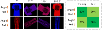
Figure 3: Illustration of RCF-MNIST

Synthetic Dataset with Subpopulation Shift. Similar to synthetic datasets with subpopulation shifts in classification, e.g., ColoredMNIST [4], we build a synthetic regression dataset – RCFashion-MNIST (RCF-MNIST), which is illustrated in Figure 3. Built on the FashionMNIST [18], the goal of RCF-MNIST is to predict the angle of rotation for each object. As shown in Figure 3, we color each image with a color between red and blue. There is a spurious correlation between angle (label) and color in training set. The larger the angle, the more red the color. In test set, we reverse spurious correlations to simulate distribution shift. We provide detailed description in Appendix E.1.

Real-world Datasets with Domain Shifts. In the following, we briefly discuss the real-world datasets with domain shifts; the detailed data descriptions in Appendix E.1: (1) PovertyMap [34] is a satellite image regression dataset, aiming to estimate asset wealth in countries that are not shown in the training set. (2) Communities and Crime (Crime) [56] is a tabular dataset, where the problem is to predict total number of violent crimes per 100K population and we aim to generalize the model to unseen states. (3) SkillCraft1 Master Table (SkillCraft) [6] is a tabular dataset, aiming to predict the mean latency from the onset of a perception action cycles to their first action in milliseconds. Here, “LeagueIndex" is treated as domain information. (4) Drug-target Interactions (DTI) [28] is aiming to predict out-of-distribution drug-target interactions in 2019-2020 after training on 2013-2018.

Comparisons and Experimental Setups. To evaluate the out-of-distribution robustness of C-Mixup, we compare it with nine invariant learning approaches that can be adapted to regression tasks, including ERM, IRM [4], IB-IRM [1], V-REx [39], CORAL [41], DRNN [16], GroupDRO [58], Fish [59], and mixup. All approaches use the same backbone model, where we adopt ResNet-50, three-layer full connected network, and DeepDTA [51] for Poverty, Crime and SkillCraft, and DTI, respectively. Following the original papers of PovertyMap [78] and DTI [28], we use $R$ value to evaluate the performance. For RCF-MNIST, Crime and SkillCraft, we use RMSE as the evaluation metric. In datasets with domain shifts, we report both average and worst-domain (primary metric for PovertyMap [34]) performance. Detailed hyperparameters are listed in Appendix E.2.

Table 3: Results for out-of-distribution robustness. We report the average and worst-domain (primary metric) performance here and the full results are listed in Appendix E.3. Sub. Shift means Subpopulation Shift. Higher $R$ or lower RMSE represent better performance. mixup and C-Mixup uses the same type of mixup variants reported in Table E.2. For PovertyMap, most results are copied from WILDS benchmark [34] and worst-domain performance is the primary metric. We bold the best results and underline the second best results.

	Sub. Shift	Domain Shift
	RCF-MNIST	PovertyMap ($R$)		Crime (RMSE)		SkillCraft (RMSE)		DTI ($R$)
	Avg. (RMSE) $\downarrow$	Avg. $\uparrow$	Worst $\uparrow$	Avg. $\downarrow$	Worst $\downarrow$	Avg. $\downarrow$	Worst $\downarrow$	Avg. $\uparrow$	Worst $\uparrow$
ERM	0.162	0.80	0.50	0.134	0.173	5.887	10.182	0.464	0.429
IRM	0.153	0.77	0.43	0.127	0.155	5.937	7.849	0.478	0.432
IB-IRM	0.167	0.78	0.40	0.127	0.153	6.055	7.650	0.479	0.435
V-REx	0.154	0.83	0.48	0.129	0.157	6.059	7.444	0.485	0.435
CORAL	0.163	0.78	0.44	0.133	0.166	6.353	8.272	0.483	0.432
GroupDRO	0.232	0.75	0.39	0.138	0.168	6.155	8.131	0.442	0.407
Fish	0.263	0.80	0.30	0.128	0.152	6.356	8.676	0.470	0.443
mixup	0.176	0.81	0.46	0.128	0.154	5.764	9.206	0.465	0.437
C-Mixup (Ours)	0.146	0.81	0.53	0.123	0.146	5.201	7.362	0.498	0.458

Results. We report both average and worst-domain performance in Table 3. According to the results, we can see that the performance of prior invariant learning approaches is not stable across datasets. For example, IRM and CORAL outperform ERM on Camelyon17, but fail to improve the performance on PovertyMap. C-Mixup instead consistently shows the best performance regardless of the data types, indicating its effeacy in improving robustness to covariate shift.

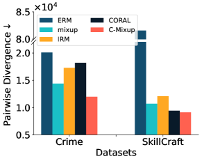
Figure 4: Results of invariance analysis. Smaller pairwise divergence value represents stronger invariance.

Analysis of Learned Invariance. Following Yao et al. [76], we analyze the domain invariance of the model learned by C-Mixup. For regression, we measure domain invariance as pairwise divergence of the last hidden representation. Since the labels are continuous, we first evenly split examples into $\mathcal{C}=\{1,\ldots,C\}$ bins according to their labels, where $C=10$. After splitting, we perform kernel density estimation to estimate the probability density function $P(h_{e}^{c})$ of the last hidden representation. We calculate the pairwise divergence as $\mathrm{Inv}=\frac{1}{|\mathcal{C}||\mathcal{E}|^{2}}\sum_{c\in\mathcal{C}}\sum_{e^{\prime},e\in\mathcal{E}}\mathrm{KL}(P(g_{E}^{c}\mid E=e)|P(g_{E}^{c}\mid E=e^{\prime}))$. The results on Crime and SkillCraft are reported in Figure 4, where smaller number denotes stronger invariance. We observe that C-Mixup learns better invariant representation compared to prior invariant learning approaches.

5.4 Analysis of C-Mixup

In this section, we conduct three analyses including the compatibility of C-Mixup, alternative distance metrics, and sensitivity of bandwidth. In Appendix F.3.2 and F.4, we analyze the sensitivity of hyperparameter $\alpha$ in Beta distribution and the robustness of C-Mixup to label noise, respectively.

Table 4: Compatibility analysis. See Appendix F.1 for full results.

Model		RCF-MNIST	PovertyMap
		RMSE $\downarrow$	Worst $R$ $\uparrow$
CutMix		0.194	0.46
	+C-Mixup	0.186	0.53
PuzzleMix		0.159	0.47
	+C-Mixup	0.150	0.50
AutoMix		0.152	0.49
	+C-Mixup	0.146	0.53

I. Compatibility of C-Mixup. C-Mixup is a complementary approach to vanilla mixup and its variants, where it changes the probabilities of sampling mixing pairs instead of changing the way to mixing. We further conduct compatibility analysis of C-Mixup by integrating it to three representative mixup variants – PuzzleMix [32], CutMix [81], AutoMix [45]. We evaluate the performance on two datasets (RCF-MNIST, PovertyMap). The reported results in Table 4 indicate the compatibility and efficacy of C-Mixup in regression.

Table 5: Performance of different distance metrics. $x$, $y$, $h$ represent input feature, label, and hidden representation, respectively. The full results are listed in Appendix F.2.

Model	Ex.-Rate	Shape1D	DTI
	RMSE $\downarrow$	MSE $\downarrow$	Avg. $R$ $\uparrow$
ERM/MAML	0.0236	4.698	0.464
mixup/MetaMix	0.0239	4.275	0.465
$d(x_{i},x_{j})$	0.0212	4.539	0.478
$d(x_{i}\oplus y_{i},x_{j}\oplus y_{j})$	0.0212	4.395	0.484
$d(h_{i},h_{j})$	0.0213	4.202	0.483
$d(h_{i}\oplus y_{i},h_{j}\oplus y_{j})$	0.0208	4.176	0.487
$d(y_{i},y_{j})$ (C-Mixup)	0.0203	4.024	0.498

II. Analysis of Distance Metrics. Besides the theoretical analysis, here we empirically analyze the effectiveness of using label distance. Here, we use $d(a,b)$ to denote the distance between objects $a$ and $b$, e.g., $d(y_{i},y_{j})$ in our case. We consider four substitute distance metrics, including: (1) feature distance: $d(x_{i},x_{j})$; (2) feature and label distance: we concatenate the input feature $x$ and label $y$ to compute the distance, i.e., $d(x_{i}\oplus y_{i},x_{j}\oplus y_{j})$; (3) representation distance: since using feature distance may fail to capture high-level feature relations, we propose to use the model’s hidden representations to measure the distance $d(h_{i},h_{j})$, detailed in Appendix F.2. (4) representation and label distance: $d(h_{i}\oplus y_{i},h_{j}\oplus y_{j})$.

The results are reported in Table 5. We find that (1) feature distance $d(x_{i},x_{j})$ does benefit performance compared with ERM and vanilla mixup in all cases since it selects more reasonable example pairs for mixing; (2) representation distance $d(h_{i},h_{j})$ outperforms feature distance $d(x_{i},x_{j})$ since it captures high-level features; (3) though involving label in representation distance is likely to overwhelm the effect of labels, the better performance of $d(h_{i}\oplus y_{i},h_{j}\oplus y_{j})$ over $d(h_{i},h_{j})$ indicates the effectiveness of regression labels in measuring example distance, which is further verified by the superiority of C-Mixup. (4) Our discussion of computational efficiency in Appendix A.3 indicates that C-Mixup is much more computationally efficient than other distance measurements.

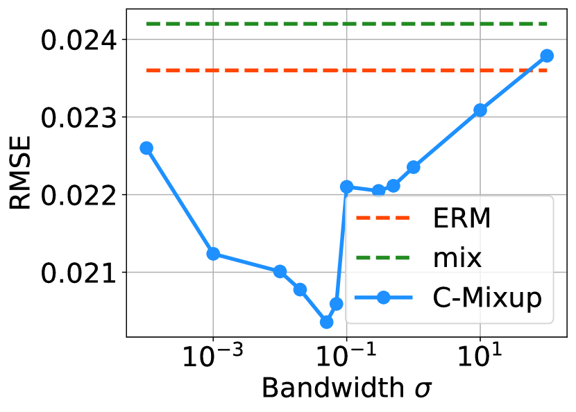
(a) : Exchange-Rate

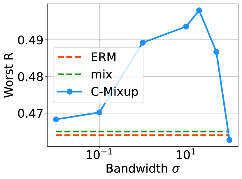
(b) : DTI

Figure 5: Sensitivity analysis of bandwidth. mix represents the better mixing approach between mixup and Manifold Mixup.

III. How does the choice of bandwidth affects the performance? Finally, we analyze the effects of the bandwidth $\sigma$ in Eqn. (6). The performance with respect to bandwidth of Exchange-Rate and DTI are visualized in Figure 5, respectively. We point out that if the bandwidth is too large, the results are close to vanilla mixup or Manifold Mixup, depending on which one is used. Otherwise, the results are close to ERM if the bandwidth is too small. According to the results, we see that the improvements of C-Mixup is somewhat stable over different bandwidths. Most importantly, C-Mixup yields a good model for a wide range of bandwidths, which reduces the efforts to tune the bandwidth for every specific dataset. Additionally, we provide empirical guidance about how to pick suitable bandwidth in Appendix F.3.1.

6 Related Work

Data Augmentation and Mixup. Various data augmentation strategies have been proposed to improve the generalization of deep neural networks, including directly augmenting images with manually designed strategies (e.g., whitening, cropping) [37], generating more examples with generative models [3, 7, 88, 85], and automatically finding augmentation strategies [10, 11, 43]. Mixup [82] and its variants [9, 12, 20, 24, 26, 32, 33, 44, 45, 52, 66, 67, 68, 81, 87] propose to improve generalization by linear interpolating input features of a pair of examples and their corresponding labels. Though mixup and its variants have demonstrated their power in classification [82], sequence labeling [84], and reinforcement learning [70], systematic analysis of mixup on different regression tasks is still underexplored. The recent MixRL [29] learns a policy network to select nearby example pairs for mixing, which requires substantial computational resources and is not suitable to high-dimensional real-world data. Unlike this method, C-Mixup instead adjusts the sampling probability of mixing pairs based on label similarity, which makes it much more efficient. Furthermore, C-Mixup, which focuses on how to select mixing examples, is a complementary method over mixup and its representative variants (see more discussion in Appendix A.4). Empirically, our experiments show the effectiveness and compatibility of C-Mixup on multiple regression tasks in Section 5.1.

Task Generalization. Our experiments extended C-Mixup to gradient-based meta-learning, aiming to improve task generalization. In the literature, there are two lines of related works. The first line of research directly imposes regularization on meta-learning algorithms [21, 30, 63, 79]. The second line of approaches introduces task augmentation to produce more tasks for meta-training, including imposing label noise [55], mixing support and query sets in the outer-loop optimization [49, 74], and directly interpolating tasks to densify the entire task distribution [77]. C-Mixup is complimentary to the latter mixup-based task augmentation methods. Furthermore, Section 5.2 indicates that C-Mixup empirically outperforms multiple representative prior approaches [79, 55].

Out-of-Distribution Robustness. Many recent methods aim to build machine learning models that are robust to distribution shift, including learning invariant representations with domain alignment [17, 41, 42, 46, 65, 72, 80, 86] or using explicit regularizers to finding a invariant predictors that performs well over all domains [1, 4, 23, 31, 36, 39, 75]. Recently, LISA [76] cancels out domain-associated correlations and learns invariant predictors by mixing examples either with the same label but different domains or with the same domain but different labels. While related, C-Mixup can be considered as a more general version of LISA that can be used for regression tasks. Besides, unlike LISA, C-Mixup do not use domain annotations, which are often expensive to obtain.

7 Conclusion

In this paper, we proposed C-Mixup, a simple yet effective variant of mixup that is well-suited to regression tasks in deep neural networks. Specifically, C-Mixup adjusts the sampling probability of mixing example pairs by assigning higher probability to pairs with closer label values. Both theoretical and empirical results demonstrate the promise of C-Mixup in improving in-distribution generalization, task generalization, and out-of-distribution robustness.

Theoretical future work may relax the assumptions in our theoretical analysis and extend the results to more complicated scenarios. We also plan to analyze more properties of C-Mixup theoretically, e.g., the relation between C-Mixup and manifold intrusion [22] in regression. Empirically, we plan to investigate how C-Mixup performs in more diverse application tasks such as semantic segmentation, natural language understanding, reinforcement learning.

Checklist

1. For all authors…

   1. Do the main claims made in the abstract and introduction accurately reflect the paper’s contributions and scope? [Yes]

   2. Did you describe the limitations of your work? [Yes] See Appendix G

   3. Did you discuss any potential negative societal impacts of your work? [N/A] C-Mixup is a general machine learning method and we believe that it has no potential negative societal impacts.

   4. Have you read the ethics review guidelines and ensured that your paper conforms to them? [Yes]

2. If you are including theoretical results…

   1. Did you state the full set of assumptions of all theoretical results? [Yes] See Section 3 and Appendix B

   2. Did you include complete proofs of all theoretical results? [Yes] See Appendix B

3. If you ran experiments…

   1. Did you include the code, data, and instructions needed to reproduce the main experimental results (either in the supplemental material or as a URL)? [Yes] See the code in https://github.com/huaxiuyao/C-Mixup

   2. Did you specify all the training details (e.g., data splits, hyperparameters, how they were chosen)? [Yes] See Appendix C.2, D.2, and E.2.

   3. Did you report error bars (e.g., with respect to the random seed after running experiments multiple times)? [Yes] See Appendix C, D, E, F.

   4. Did you include the total amount of compute and the type of resources used (e.g., type of GPUs, internal cluster, or cloud provider)? [Yes] See Appendix C.2, D.2, and E.2.

4. If you are using existing assets (e.g., code, data, models) or curating/releasing new assets…

   1. If your work uses existing assets, did you cite the creators? [Yes]

   2. Did you mention the license of the assets? [Yes]

   3. Did you include any new assets either in the supplemental material or as a URL? [Yes] See the code in https://github.com/huaxiuyao/C-Mixup

   4. Did you discuss whether and how consent was obtained from people whose data you’re using/curating? [N/A]

   5. Did you discuss whether the data you are using/curating contains personally identifiable information or offensive content? [N/A]

5. If you used crowdsourcing or conducted research with human subjects…

   1. Did you include the full text of instructions given to participants and screenshots, if applicable? [N/A]

   2. Did you describe any potential participant risks, with links to Institutional Review Board (IRB) approvals, if applicable? [N/A]

   3. Did you include the estimated hourly wage paid to participants and the total amount spent on participant compensation? [N/A]

Appendix A Additional Information for C-Mixup

A.1 Illustration of How C-Mixup Improves Out-of-Distribution Robustness

In Figure 6, we use the ShapeNet1D to illustrate how C-Mixup improves out-of-distribution robustness. Here, we color the images to construct different domains. We train the model on red and blue domains and then generalize it to the green one. In Figure 6, we can see that C-Mixup can recognize more reasonable mixing pairs compared with vanilla mixup. Mixup with feature similarity fails to cancel out the domain information since it may be easier to mix unreasonable example pairs within the same domain. C-Mixup instead is naturally suitable to average out domain information by mixing examples with close labels.

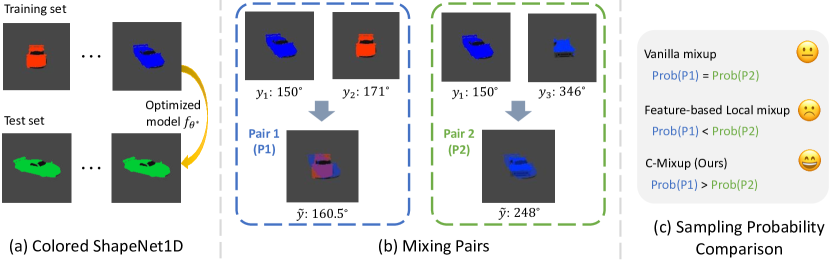
Figure 6: Illustration of C-Mixup for out-of-distribution robustness. Here, we color the ShapeNet1D and regard color as the domain information. $\lambda$ represents the interpolation ratio. (a) Colored ShapeNet1D pose prediction task, aiming to generalize the model trained on red and blue domains to the green domain; (b) Two mixing pairs with interpolated images and labels; (c) Illustration of a rough comparison of sampling probabilities between two mixing pairs in (b). Here, C-Mixup is capable of assigning higher sampling probability to more reasonable pairs and eliminate the effect of domain information.

A.2 Algorithm of Meta-Training with C-Mixup

In this section, we summarize the algorithm of applying C-Mixup to MetaMix [74] in Alg. 2. Here, we adopt MetaMix with mixup version, which could be easily adapted to other mixup variants (e.g., CutMix, Manifold Mixup)

Algorithm 2 Meta-Training Process of MetaMix with C-Mixup

0:  Outer-loop learning rate $\eta$; Inner-loop learning rate $\xi$ (we change $\alpha$ in Eqn. (4) of the main paper to $\xi$ to avoid notation conflict); Shape parameter $\alpha$; Task distribution $p(\mathcal{T})$

1:  Randomly initialize model parameters $\theta$

2:  while not converge do

3:     Sample a batch of tasks $\{\mathcal{T}_{i}\}_{i=1}^{|M|}$ with the corresponding dataset $\mathcal{D}_{m}$

4:     for all $\mathcal{T}_{m}$ do

5:        Sample a support set $\mathcal{D}_{m}^{s}$ and a query set $\mathcal{D}_{m}^{q}$ from $\mathcal{D}_{m}$

6:        Calculate pairwise distance matrix $P$ between query set and support set via Eqn. (6).

7:        Calculate the task-specific parameter $\phi_{m}$ via the inner-loop gradient descent, i.e., $\phi_{m}=\theta-\xi\nabla_{\theta}\mathcal{L}(f_{\theta};\mathcal{D}_{m}^{s})$

8:        for each query example ($x_{m,i}^{q},y_{m,i}^{q}$) do

9:           Sample MetaMix parameter $\lambda\sim\mathrm{Beta}(\alpha,\alpha)$

10:           Sample support set example ($x_{m,j}^{s}$, $y_{m,j}^{s}$) according to the probability $P(\cdot\mid(x_{m,i}^{q},y_{m,i}^{q}))$

11:           Linearly interpolate ($x_{m,i}^{q}$, $y_{m,i}^{q}$) and ($x_{m,j}^{s}$, $y_{m,j}^{s}$) to get ($\tilde{x}_{m,i}^{q},\tilde{y}_{m,i}^{q}$)

12:           Replace ($x_{m,i}^{q},y_{m,i}^{q}$) with ($\tilde{x}_{m,i}^{q},\tilde{y}_{m,i}^{q}$)

13:     Use interpolated examples to update the model via $\theta\leftarrow\theta-\eta\frac{1}{|M|}\sum_{i=1}^{|M|}\mathcal{L}(f_{\phi_{m}};\tilde{\mathcal{D}}_{m}^{q})$

A.3 Efficiency Discussion of C-Mixup

Assume the number of examples are $n$, the dimension of features and labels are $M_{f}$ and $M_{l}$, respectively. The time complexity of calculating the pairwise distance matrix $P$ with feature distance or label distance is $O(n^{2}M_{f})$ or $O(n^{2}M_{l})$, respectively. Generally, since $M_{l}\ll M_{f}$, using label distance (i.e., C-Mixup) substantially reduces the cost of calculating the pairwise distance matrix.

Algorithm 3 Training with C-Mixup-batch

0:  Learning rates $\eta$; Shape parameter $\alpha$

0:  Training data $\mathcal{D}:=\{(x_{i},y_{i})\}_{i=1}^{N}$

1:  Randomly initialize model parameters $\theta$

2:  while not converge do

3:     Sample two batches of examples $\mathcal{B}_{1},\mathcal{B}_{2}\sim\mathcal{D}$

4:     Calculate pairwise distance matrix $P$ between $\mathcal{B}_{1}$ and $\mathcal{B}_{2}$ via Eqn. (6)

5:     for each example $(x_{i},y_{i})\in\mathcal{B}_{1}$ do

6:        Sample example ($x_{j}$, $y_{j}$) from $\mathcal{B}_{2}$ according to the probability $P(\cdot\mid(x_{i},y_{i}))$

7:        Sample $\lambda$ from $\mathrm{Beta}(\alpha,\alpha)$

8:        Linearly interpolate ($x_{i}$, $y_{i}$) and ($x_{j}$, $y_{j}$) to get ($\tilde{x},\tilde{y}$)

9:     Use interpolated examples to update the model via Eqn. (3)

Furthermore, the calculation of pairwise distance matrix can be accelerated using parallelized operations, but it is still challenging if $n$ is sufficiently large, e.g., billions of examples. We thus propose an alternative solution that applies C-Mixup only to every example batch, which is named as C-Mixup-batch. In Alg. 3, we summarize the training process of C-Mixup-batch. We compare C-Mixup and C-Mixup-batch, and report the results of in-distribution generalization and out-of-distribution robustness in Table 6 and Table 7, respectively. Notice that we have used C-Mixup-batch for Echo, RCF-MNIST, ProvertyMap since calculating pair-wise distance metrics for these large datasets is time-consuming. Hence, we only report the results for other datasets. According to the results, we observe that C-Mixup-batch achieves comparable performance to C-Mixup. Nevertheless, the downside of C-Mixup-batch is that we must calculate the pairwise distance matrix for every batch. Accordingly, original C-Mixup is suitable to most datasets, while C-Mixup-batch is more appropriate to large datasets (e.g., Echo).

Table 6: Comparison between C-Mixup and C-Mixup-batch to in-distribution generalization. Since Echo is a large dataset and C-Mixup-batch is used by default, we only report the results of Airfoil, NO2, Exchange-Rate and Electricity here.

	Dataset	Airfoil	NO2	Exchange-Rate	Electricity
RMSE $\downarrow$	C-Mixup-batch	2.792 $\pm$ 0.135	0.510 $\pm$ 0.007	0.0205 $\pm$ 0.0017	0.0576 $\pm$ 0.0002
	C-Mixup	2.717 $\pm$ 0.067	0.509 $\pm$ 0.006	0.0203 $\pm$ 0.0011	0.0570 $\pm$ 0.0006
MAPE $\downarrow$	C-Mixup-batch	1.616 $\pm$ 0.053%	12.894 $\pm$ 0.180%	2.064 $\pm$ 0.218%	13.697 $\pm$ 0.155%
	C-Mixup	1.610 $\pm$ 0.085%	12.998 $\pm$ 0.271%	2.041 $\pm$ 0.134%	13.372 $\pm$ 0.106%

Table 7: Comparison between C-Mixup and C-Mixup-batch to out-of-distribution robustness. Since we have applied C-Mixup-batch to PovertyMap, we report the results of Crime, SkillCraft, DTI.

	Dataset	Crime (RMSE $\downarrow$)	SkillCraft (RMSE $\downarrow$)	DTI ($R\uparrow$)
Avg	C-Mixup-batch	0.125 $\pm$ 0.001	5.619 $\pm$ 0.212	0.490 $\pm$ 0.005
	C-Mixup	0.123 $\pm$ 0.000	5.201 $\pm$ 0.059	0.498 $\pm$ 0.008
Worst	C-Mixup-batch	0.152 $\pm$ 0.007	7.665 $\pm$ 0.875	0.453 $\pm$ 0.006
	C-Mixup	0.146 $\pm$ 0.002	7.362 $\pm$ 0.244	0.458 $\pm$ 0.004

A.4 Discussion between C-Mixup and Mixup

In this paper, we regard C-Mixup is an complementary approach to mixup and its most representative variants (e.g., Manifold Mixup [68], CutMix [81]). Here, we use vanilla mixup as an exemplar to show the difference. According to our description of mixup in Section 2 of the main paper, the entire mixup process includes three stages:

• Stage I: sample two instances ($x_{i}$, $y_{i}$), ($x_{j}$, $y_{j}$) from the training set.

• Stage II: sample the interpolation factor $\lambda$ from the Beta distribution Beta($\alpha$, $\alpha$).

• Stage III: mixing the sampled instances with interpolation factor $\lambda$ according to the following mixing formulation:

  $$x_{mix}=\lambda x_{i}+(1-\lambda)x_{j},y_{mix}=\lambda y_{i}+(1-\lambda)y_{j},\lambda\sim\mathrm{Beta}(\alpha,\alpha).$$

In the original mixup, the interpolation factor $\lambda$ sampled in the stage II controls how to mix these two instances. C-Mixup instead manipulates stage I and pairs with closer labels are more likely to be sampled.

In addition to the discussion of the complementarity of C-Mixup, the original mixup paper further shows that randomly interpolating examples from the same label performs worse than completely random mixing examples in classification. Compared to classification, randomly mixing examples in regression may be easier to generate semantically wrong labels. Intuitively, linearly mixing one-hot labels in classification is easy to generate semantically meaningful artificial labels, where the mixed label represents the probabilities of mixed examples to some extent. While in regression, the mixed labels may be semantically meaningless (e.g., pairs 2 and 3 in Figure 1) and more significantly affect the performance. By mixing examples with closer labels, C-Mixup mitigates the influence of semantically wrong labels and improves the in-distribution and task generalization in regression. Additionally, C-Mixup further shows its superiority in improving out-of-distribution robustness in regression, which is not discussed in the original mixup paper.

Appendix B Detailed Proofs

In this section, we provide detailed proofs of Theorem 1, 2, 3. To avoid symbol conflict, we would like to point out that we use $h$ to denote the bandwidth of kernel in the nonparametric estimation step, which is different from the bandwidth $\sigma$ in Eqn. (6) of the main paper, which was used to measure the similarity in mixup. In Section B.4, we provide proofs for all used Lemmas.

B.1 Proof of Theorem 1

We first state the kernel estimator.

$$\hat{g}(t;\theta)=\frac{\sum_{i=1}^{n}K(\theta^{\top}x_{i},t)y_{i}}{\sum_{i=1}^{n}K(\theta^{\top}x_{i},t)},$$

this kernel function can take, for example, the uniform kernel function $K(t_{1},t_{2})=1\{|t_{1}-t_{2}|<h\}$ or a Gaussian kernel function $K(t_{1},t_{2})=\exp(-|t_{1}-t_{2}|^{2}/h^{2})$ where $h$ is the bandwidth.

To make the proof easier to follow, we restate Theorem 1 below.

Theorem 1.

Suppose $\theta\in\mathbb{R}^{p}$ is sparse with sparsity $s=o(\min\{p,\sigma_{\xi}^{2}\})$, $p=o(N)$ and $g$ is smooth with $c_{0}<g^{\prime}<c_{1}$, $c_{2}<g^{\prime\prime}<c_{3}$ for some universal constants $c_{0},c_{1},c_{2},c_{3}>0$. There exists a distribution on $x$ with a kernel function, such that when the sample size $N$ is sufficiently large, with probability $1-o(1)$,

$$\small\mathrm{MSE}(\theta^{*}_{C-Mixup})<\min(\mathrm{MSE}(\theta^{*}_{feat}),\mathrm{MSE}(\theta^{*}_{mixup})).$$ (12)

Proof. For identifiability, we consider the case where $\theta$ has $\ell_{2}$ norm of 1. Let us construct the distribution of $x$ as $z\sim\frac{1}{K}\sum_{k=1}^{K}N_{p}(\mu_{k},\sigma_{z}^{2}I_{p})$ with $\mu_{k}=\frac{k}{\|\theta\|}\theta$ for a fixed positive integer $K$. We break out the entire proof into three steps.

Step 1. We first analyze the behavior of the three mixup methods. First, we have

$$\theta^{\top}z\sim\frac{1}{K}\sum_{k=1}^{K}N_{p}(\mu_{k}^{\top}\theta,\sigma_{z}^{2}\|\theta\|^{2}),$$

and

$$\theta^{\top}\xi\sim\frac{1}{K}\sum_{k=1}^{K}N_{p}(0,\sigma_{\xi}^{2}\|\theta\|^{2}).$$

We then have

$$|y_{k^{\prime}}-y_{k}|=|g(\mu_{k}^{\top}\theta)-g(\mu_{k^{\prime}}^{\top}\theta)|\pm\Theta((\sigma_{\xi}+\sigma_{x})\|\theta\|)=|g(k)-g(k^{\prime})|\pm\Theta((\sigma_{\xi}+\sigma_{x})\|\theta\|)$$

$$\|x_{k^{\prime}}-x_{k}\|=\|\mu_{k}-\mu_{k}^{\prime}\|\pm\Theta((\sigma_{\xi}+\sigma_{x})\cdot\sqrt{d})=|k-k^{\prime}|\pm\Theta((\sigma_{\xi}+\sigma_{x})\cdot\sqrt{d})$$

As a result, if we take $(\sigma_{\xi}+\sigma_{x})\|\theta\|=o(1)$, and $(\sigma_{\xi}+\sigma_{x})\cdot\sqrt{d}\to\infty$, C-Mixup only interpolates examples within the same cluster, while mixup with feature similarity and vanilla mixup interpolate examples across different clusters.

Step 2. We then show that $\hat{\theta}$ obtained by all the three methods is consistent (the estimation error goes to 0 when the sample size goes to infinity). We first present a lemma showing that in expectation, the solution would recover $\theta$.

Lemma 1.

Suppose $x_{i}$’s are i.i.d. sampled from $N_{p}(\mu,I)$, then we have

$$\mathbb{E}[y_{i}x_{i}]=(\mathbb{E}[g^{\prime}(x_{i}^{\top}\theta)]+\mathbb{E}[g(x_{i}^{\top}\theta)])\cdot\theta.$$

The proof of Lemma 1 is deferred to Section B.4.

This lemma implies that if $\tilde{x}=\lambda x_{k}+(1-\lambda)x_{k}^{\prime}$, $\tilde{y}=\lambda y_{k}+(1-\lambda)y_{k}^{\prime}$, we have

$$\mathbb{E}[\tilde{y}\tilde{x}]=c_{k,k^{\prime}}\theta,$$

for some constant $c_{k,k^{\prime}}$. Additionally, we have $\mathbb{E}[\tilde{x}\tilde{x}^{\top}]=cI+c^{\prime}_{k,k^{\prime}}\theta\theta^{\top}$. Therefore, $\mathbb{E}[\tilde{x}\tilde{x}^{\top}]^{-1}\mathbb{E}[\tilde{y}\tilde{x}]=\tilde{c}_{k,k^{\prime}}\theta$ (via the Sherman–Morrison formula), for some constant $\tilde{c}_{k,k^{\prime}}$.

Since we assume $g$ is $c_{1}$-Lipschitz for some universal constant $c_{1}$, which also implies $\tilde{c}_{k,k^{\prime}}=O(1)$. We then analyze the convergence of $\hat{\theta}$. By definition, we have

$$\hat{\theta}=(\frac{1}{N}\sum_{i=1}^{N}\tilde{x}_{i}\tilde{x}_{i}^{\top})^{-1}(\frac{1}{N}\sum_{i=1}^{N}\tilde{x}_{i}\tilde{y}_{i}).$$

Using Bernstein inequality, we have with probability at least $1-p^{-2}$,

$$\|\frac{1}{N}\sum_{i=1}^{N}\tilde{x}_{i}\tilde{x}_{i}^{\top}-\mathbb{E}[\tilde{x}\tilde{x}^{\top}]\|=O(\sqrt{\frac{p}{N}}),$$

and

$$\|\frac{1}{N}\sum_{i=1}^{N}\tilde{x}_{i}\tilde{y}_{i}-\mathbb{E}[\tilde{x}\tilde{y}]\|=O(\sqrt{\frac{p}{N}}).$$

Then using Lemma 1, since $\lambda_{\min}(\mathbb{E}[\tilde{x}\tilde{x}^{\top}])\gtrsim c_{1}$, when $n$ is sufficiently large, we then have

$$\|\hat{\theta}-\theta\|_{2}\lesssim\sqrt{\frac{p}{N}}=o(1).$$

Step 3. We finally proceed to the nonparametric estimation step.

For C-Mixup, since we only interpolates the samples within the same Gaussian cluster, using the fact that $\sigma_{\xi}=o(1)$, $K$ being Lipschitz, and $\|\hat{\theta}-\theta\|_{2}=o(1)$, we have that

$$\|\hat{g}(t;\hat{\theta})-\frac{\sum_{i=1}^{N}K(z_{i}^{\top}\theta,t)y_{i}}{\sum_{i=1}^{N}K(z_{i}^{\top}\theta,t)}\|=\|\frac{\sum_{i=1}^{N}K(x_{i}^{\top}\hat{\theta},t)y_{i}}{\sum_{i=1}^{N}K(x_{i}^{\top}\hat{\theta},t)}-\frac{\sum_{i=1}^{N}K(z_{i}^{\top}\theta,t)y_{i}}{\sum_{i=1}^{N}K(z_{i}^{\top}\theta,t)}\|=o(1),$$ (13)

here the function norm of $h$ is defined as $\|h\|=\sqrt{\mathbb{E}[h^{2}(x)]}.$

Using the standard nonparametric regression results (e.g., see Tsybakov [64]), when the feature is observed without noise, the kernel estimator is consistent:

$$\|g(t)-\frac{\sum_{i=1}^{N}K(z_{i}^{\top}\theta,t)y_{i}}{\sum_{i=1}^{N}K(z_{i}^{\top}\theta,t)}\|=o(1).$$ (14)

Combining the two inequalities (13) and (14), we find that the $\hat{g}$ obtained by C-Mixup satisfies

$$\|\hat{g}-g\|=o(1).$$

For vanilla mixup and mixup with feature similarity, we have show that with a nontrivial positive probability, the samples are from two different clusters. Therefore using the assumption on $g^{\prime}$ and $g^{\prime\prime}$, we have $\tilde{y}-y_{i}\geq c$ for some constant $c>0$ with Jensen’s inequality. As a result,

$$|\frac{\sum_{i=1}^{N}K(x_{i}^{\top}\hat{\theta},t)y_{i}}{\sum_{i=1}^{N}K(x_{i}^{\top}\hat{\theta},t)}-\frac{\sum_{i=1}^{N}K(x_{i}^{\top}\hat{\theta},t)\tilde{y}_{i}}{\sum_{i=1}^{N}K(x_{i}^{\top}\hat{\theta},t)}|\geq c.$$

Combining with the two inequalities (13) and (14), we have the $\hat{g}$ obtained by vanilla mixup or mixup with feature similarity satisfies

$$\|\hat{g}-g\|>c.$$

Since $\mathrm{MSE}(\theta)\asymp\|\hat{g}(\cdot;\theta)-g(\cdot)\|$, we then have

$$\small\mathrm{MSE}(\theta^{*}_{C-Mixup})<\min(\mathrm{MSE}(\theta^{*}_{feat}),\mathrm{MSE}(\theta^{*}_{mixup})).$$

B.2 Proof of Theorem 2

We first restate Theorem 2.

Theorem 2.

Let $N=\sum_{m=1}^{M}N_{m}$ and $N_{m}$ is the number of examples of $\mathcal{T}_{m}$. Suppose $\theta_{k}$ is sparse with sparsity $s=o(\min\{d,\sigma_{\xi}^{2}\})$, $p=o(N)$ and $g_{m}$’s are smooth with $0<g_{m}^{\prime}<c_{1}$, $c_{2}<g_{m}^{\prime\prime}<c_{3}$ for some universal constants $c_{1},c_{2},c_{3}>0$ and $m\in[M]\cup\{t\}$. There exists a distribution on $x$ with a kernel function, such that when the sample size $N$ is sufficiently large, with probability $1-o(1)$,

$$\small\mathrm{MSE}_{\mathrm{Target}}(\theta^{*}_{Meta-C-Mixup})<\min(\mathrm{MSE}_{\mathrm{Target}}(\theta^{*}_{Meta-feat}),\mathrm{MSE}_{\mathrm{Target}}(\theta^{*}_{MetaMix})).$$ (15)

Again, we consider the distribution of $x$ to be $z\sim\frac{1}{K}\sum_{k=1}^{K}N_{p}(\mu_{k},\sigma_{z}^{2}I_{p})$ with $\mu_{k}=\frac{k}{\|\theta\|}\theta$ for a fixed positive integer $K$. The proof of Theorem 2 largely follows Theorem 1, with the only difference in the step 2. We prove the step 2 for Theorem 2 in the following.

By Lemma 1, for augmented data in the $m$-th task, $\tilde{x}^{(m)}=\lambda x_{k}^{(m)}+(1-\lambda)x_{k}^{(m)^{\prime}}$, $\tilde{y}^{(m)}=\lambda y_{k}^{(m)}+(1-\lambda)y^{(m)^{\prime}}_{k}$, we have

$$\mathbb{E}[\tilde{y}^{(m)}\tilde{x}^{(m)}]=c^{(m)}_{k,k^{\prime}}\theta,$$

for some constant $c^{(m)}_{k,k^{\prime}}$.

Additionally, we have $\mathbb{E}[\tilde{x}^{(m)}\tilde{x}^{(m)\top}]=c^{(m)}I+c^{(m)^{\prime}}_{k,k^{\prime}}\theta\theta^{\top}$. Therefore, $(\sum_{m=1}^{T}\mathbb{E}[\tilde{x}^{(m)}\tilde{x}^{(m)\top}])^{-1}(\sum_{m=1}^{T}\mathbb{E}[\tilde{y}^{(m)}\tilde{x}^{(m)}])=\tilde{c}_{k,k^{\prime}}\theta,$ for some constant $\tilde{c}_{k,k^{\prime}}$.

We then analyze the convergence of $\hat{\theta}$. By definition, we have

$$\hat{\theta}=(\frac{1}{N}\sum_{m=1}^{T}\frac{1}{n_{m}}\sum_{i=1}^{n_{t}}\tilde{x}^{(m)}_{i}\tilde{x}_{i}^{(m)\top})^{-1}(\frac{1}{N}\sum_{m=1}^{T}\frac{1}{n_{m}}\sum_{i=1}^{n_{t}}\tilde{x}^{(m)}_{i}\tilde{y}^{(m)}_{i}).$$

Using Bernstein inequality, we have with probability at least $1-p^{-2}$,

$$\|\frac{1}{N}\sum_{m=1}^{T}\frac{1}{n_{m}}\sum_{i=1}^{n_{m}}x_{i}^{(m)}x_{i}^{(m)\top}-\frac{1}{N}\sum_{m=1}^{T}\mathbb{E}[\tilde{x}^{(m)}\tilde{x}^{(m)\top}]\|=O(\sqrt{\frac{p}{N}}),$$

and

$$\|\frac{1}{T}\sum_{m=1}^{T}\frac{1}{n_{m}}\sum_{i=1}^{n_{m}}x_{i}^{(m)}y_{i}^{(m)}-\mathbb{E}[\frac{1}{T}\sum_{t=1}^{T}\mathbb{E}[x^{(m)}y^{(m)}]]\|=O(\sqrt{\frac{p}{N}}).$$

Then using Lemma 1, when $N$ is sufficiently large, we then have

$$\|\hat{\theta}-\theta\|_{2}\lesssim\sqrt{\frac{p}{N}}=o(1).$$

B.3 Proof of Theorem 3

Similarly we restate Theorem 3.

Theorem 3.

Supposed for some $\max(\exp(-n^{1-o(1)}),\exp(-\frac{p_{1}^{2}}{2n}))<\delta\ll 1$, we have variance constraints: $\sigma_{a}=c_{1}\sigma_{x}$ , $\sigma_{x}\geq c_{2}\max(\frac{n^{5/2}}{\|{\theta}\|\delta}\sigma_{\epsilon},\frac{\sqrt{p_{2}}\|{\theta}\|}{\sqrt{n}p_{1}})$ and $\sigma_{\epsilon}^{2}\leq\frac{c_{3}}{pn^{3/2}}$ . Then for any penalty k satisfies $c_{4}\sqrt{\frac{p_{2}}{p_{1}}}n^{1/4+o(1)}<k<c_{5}\min(\frac{\sigma_{x}}{\|{\theta}\|}\sqrt{p_{1}n^{1-o(1)}},n)$ and bandwidth h satisfies $0<h\leq c_{6}\frac{l}{\sqrt{\log(n^{2}/p_{1})}}$ in C-Mixup, when $n$ is sufficiently large, with probability at least $1-o(1)$, we have

$$\small\mathrm{MSE}(\theta^{*}_{C-Mixup})<\min(\mathrm{MSE}(\theta^{*}_{feat}),\mathrm{MSE}(\theta^{*}_{mixup})),$$ (16)

where $c_{1}\geq 1$, $c_{2}$, $c_{3}$, $c_{4}$, $c_{5}$, $c_{6}$ > 0 are universal constants, $l=\min_{i\neq j}\lvert y_{i}-y_{j}^{\prime}\rvert$ and $p_{1}\ll n<p_{1}^{2}$.

Let $p=p_{1}+p_{2}$, and $\theta_{1}$ represents the subvectors that contain the first $p_{1}$ coordinates of $\theta$. Furthermore, let $\hat{X}\in\mathbb{R}^{n\times p}$ be an arbitrary noise-less data matrix and $\hat{\lambda}_{0}\geq\hat{\lambda}_{1}\geq...\geq\hat{\lambda}_{p}$ be the singular values of $\hat{X}$. Similarly, let $E\in\mathbb{R}^{n\times p}$ be the noise matrix which contains $iid.$ sub-Gaussian entries with variance proxy $\sigma_{\epsilon}^{2}$, and $\lambda_{0}\geq\lambda_{1}\geq...\geq\lambda_{p}$ be the singular values of input matrix $X=\hat{X}+E$.

Firstly we show that the noise matrix only makes a small difference between the singular values of noise-less data matrix $\hat{X}$ and that of input matrix $X$.

Lemma 2.

If $e^{-n}<\delta_{1}\ll 1$ and $\sigma_{\epsilon}^{2}\leq\frac{c}{pn^{3/2}}$, then with probability at least $1-\delta_{1}$ we have:

$$\lvert\hat{\lambda}_{u}-\lambda_{u}\rvert\leq 16cn^{-1/2},$$ (17)

for every u satisfies $1\leq u\leq p$.

Before analyzing the effectiveness of C-Mixup, we first present the following lemma to analyze the C-Mixup with truncated label distance measurements. Specifically, we only apply C-Mixup to examples within a label distance threshold.

Lemma 3.

Assume $\exp(-n^{1-o(1)})<\delta_{1}\ll 1$, $\sigma_{x}\geq c_{2}\frac{n^{5/2}}{\|{\theta}\|\delta}\sigma_{\epsilon}$ for some $c_{2}$ that satisfies $c_{gap}:=\frac{c_{2}\sqrt{\pi}}{4\sqrt{2+\lvert\theta_{1}\rvert^{2}}}>1$. Here $c_{gap}$ is the ratio of $\min_{i\neq j}\lvert y_{i}-y_{j}^{\prime}\rvert$ to $\max\limits_{i}\lvert y_{i}-y_{i}^{\prime}\rvert$. Then if we use C-Mixup, there exists some thresholds such that with probability at least $1-\delta_{1}$, the training data $(x_{i},y_{i})$ will only be mixed with $(x^{\prime}_{i},y^{\prime}_{i})$. Here, we point out that $x_{i}$ and $x_{i}^{\prime}$ are defined in Line 206-207 in the main paper.

Then we consider replacing the truncated kernel with the gaussian kernel, which applies C-Mixup to all the examples with a smoother probability distribution. And we claim that there exist some bandwidths such that the data pairs with almost identical invariant features and opposite domain-changeable features will be mixed up together with high probability.

Lemma 4.

Assume $\exp(-\frac{p_{1}^{2}}{2n})<\delta_{1}\ll 1$ and for $l=\min_{i\neq j}|y_{i}-y_{j}^{\prime}|$, we have $0<h\leq c_{6}\frac{l}{\sqrt{\log(n^{2}/p_{1})}}$ for some $c_{6}:0<c_{6}\leq c_{gap}^{-1}\sqrt{(c_{gap}^{2}-1)/4}$, where $c_{gap}$ follows the definition in Lemma 3. We define the mixed input as $\tilde{X}$, and let $S_{i}$ be a random variable that denotes if $(x_{i},y_{i})$ is mixed with $(x_{i}^{\prime},y_{i}^{\prime})$. Then with probability at least $1-\delta_{1}$, we have:

$$n-\frac{p_{1}}{2}\leq\sum_{i=1}^{n}S_{i}\leq n.$$

Next, we find that the input matrix $X$ corresponding to C-Mixup will have just $p_{1}$, rather than $p$, singular values that are much bigger than zero.

Lemma 5.

Assume the conditions of Lemma 2 and Lemma 4 still hold and the mixup ratio $\lambda=0.5$. If noise-less data matrix $\hat{X}$ is obtained by C-Mixup, then the singular values of input matrix $X$ satisfy:

$$\begin{split}(1-b(n))^{2}n\leq&\lambda_{i}\leq(1+b(n))^{2}n,\qquad 1\leq i\leq p_{1},\\ \lvert&\lambda_{i}\rvert\leq 16\frac{c}{\sqrt{n}},\ \qquad\qquad p_{1}\leq i\leq p.\end{split}$$ (18)

Finally, we can complete the proof of Theorem 3 according to the lemmas above.

Proof of Theorem 3. Denote the input matrix as $X\in\mathbb{R}^{n\times p}$ and its singular values as $\lambda_{0}\geq\lambda_{1}\geq...\geq\lambda_{p}$. Then, for ridge estimator with penalty $k$, we have Hoerl and Kennard [25] :

$$\begin{split}\mathbb{E}[\lvert\theta^{*}(k)-\theta\rvert^{2}]&=\mathbb{E}[\lvert(X^{T}X+kI)^{-1}X^{T}Y-\theta\rvert^{2}]\\ &=\sigma_{x}^{2}\sum_{i=1}^{p}\frac{\lambda_{i}}{(\lambda_{i}+k)^{2}}+k^{2}\theta^{T}(X^{T}X+kI)^{-2}\theta\\ &=\sigma_{x}^{2}\sum_{i=1}^{p_{1}}\frac{\lambda_{i}}{(\lambda_{i}+k)^{2}}+\sigma_{x}^{2}\sum_{i=p_{1}+1}^{p_{2}}\frac{\lambda_{i}}{(\lambda_{i}+k)^{2}}+k^{2}\theta^{T}(X^{T}X+kI)^{-2}\theta\\ &=\gamma_{1}(k)+\gamma_{2}(k)+\gamma_{3}(k)\end{split}$$

For the first term, we have

$$\begin{split}\gamma_{1}^{C-Mixup}(k)&=\sigma_{x}^{2}\sum_{i=1}^{p_{1}}\frac{\lambda_{i}}{(\lambda_{i}+k)^{2}}\\ &\leq\sigma_{x}^{2}\sum_{i=1}^{p_{1}}\frac{1}{(\min_{1\leq i\leq p_{1}}\lambda_{i})}\\ &\leq\frac{\sigma_{x}^{2}p_{1}}{(1-b(n))^{2}n},\qquad(\mathrm{Lemma}~{}\ref{B3_4_lemma_lambda})\end{split}$$

and

$$\gamma_{1}^{mixup}(k)\wedge\gamma_{1}^{feat}(k)\wedge\gamma_{1}^{C-Mixup}(k)\geq\sigma_{x}^{2}\sum_{i=1}^{p_{1}}\frac{1}{4k}\geq\frac{\sigma_{x}^{2}p_{1}}{4c_{5}n}.\qquad(k<c_{5}n,c_{5}\geq\frac{1}{4})$$

To bound the last term, we perform orthogonal decompose on $X^{T}X$, i.e., $X^{T}X=P^{T}\Lambda P$. $P$ is orthogonal transformation and we denote $\alpha=P\theta$. Since the last $p_{2}$ coordinates of $\theta$ are $0$, with probability at least $1-\delta_{1}$, for C-Mixup we have:

$$\gamma_{3}^{C-Mixup}(k) =k^{2}\theta^{T}(X^{T}X+kI)^{-2}\theta$$

$$=k^{2}\sum_{i=1}^{p}\frac{\alpha_{i}^{2}}{(\lambda_{i}+k)^{2}}$$

$$=\sum_{i=1}^{p_{1}}\frac{\alpha_{i}^{2}}{(\lambda_{i}/k+1)^{2}}$$

$$\leq\frac{k^{2}\lvert\theta\rvert^{2}}{(\min_{1\leq i\leq p_{1}}\lambda_{i})^{2}}\qquad(\sum_{i=1}^{p_{1}}\alpha_{i}^{2}=\lvert\theta\rvert^{2})$$

$$\leq\frac{c_{5}^{2}}{(1-b(n))^{4}n^{o(1)}}\frac{\sigma_{x}^{2}p_{1}}{n}\qquad(k<c_{5}\frac{\sigma_{x}}{\|{\theta}\|}\sqrt{p_{1}n^{1-o(1)}},\ \mathrm{Lemma}~{}\ref{B3_4_lemma_lambda}).$$

For the second term, we bound C-Mixup as

$$\begin{split}\gamma_{2}^{C-Mixup}(k)&=\sigma_{x}^{2}\sum_{i=p_{1}+1}^{p_{2}}\frac{\lambda_{i}}{(\lambda_{i}+k)^{2}}\\ &\leq\sigma_{x}^{2}\sum_{i=p_{1}+1}^{p_{2}}\frac{\lambda_{i}}{k^{2}}\\ &\leq\frac{16c}{c_{4}^{2}n^{o(1)}}\frac{\sigma_{x}^{2}p_{1}}{n}.\qquad(k>c_{4}\sqrt{\frac{p_{2}}{p_{1}}}n^{1/4+o(1)},\ \mathrm{Lemma}~{}\ref{B3_4_lemma_lambda})\end{split}$$ (19)

For mixup and mixup with feature similarity, we bound the second term as:

$$\begin{split}\gamma_{2}^{feat}(k)\wedge\gamma_{2}^{mixup}(k)&\geq\sigma_{x}^{2}\sum_{i=1}^{p_{1}}\frac{1}{4k}\geq\frac{\sigma_{x}^{2}p_{2}}{4c_{5}n}.\qquad(k<c_{5}n)\end{split}$$

Thus there exists some constants $c$, $c_{4}$, $c_{5}$ (for example, $c_{4}=4\sqrt{c}$ and $c_{5}=1/4$), such that when n is sufficiently large, with probability at least $1-o(1)$:

$$\mathbb{E}\lvert\theta_{C-Mixup}^{*}(k)-\theta\rvert^{2}<\min(\mathbb{E}\lvert\theta_{feat}^{*}(k)-\theta\rvert^{2},\mathbb{E}\lvert\theta_{mixup}^{*}(k)-\theta\rvert^{2}).$$

which can reduce to the results immediately.

B.4 Proofs of Lemmas

Proof of Lemma 1. In order to prove Lemma 1, let us invoke the First-order Stein’s Identity [61].

Lemma 6.

Let $X\in\mathbb{R}^{d}$ be a real-valued random vector with density $p$. Assume that $p$: $\mathbb{R}^{d}\to R$ is differentiable. In addition, let $g:\mathbb{R}^{d}\to\mathbb{R}$ be a continuous function such that $\mathbb{E}[\nabla g(X)]$ exists. Then it holds that

$$\mathbb{E}[g(X)\cdot S(X)]=\mathbb{E}[\nabla g(X)],$$

where $S(X)=-\nabla p(x)/p(x)$ is the score function of $p$.

Now, let us plug in the density of $N_{d_{1}}(0,\Sigma_{X})$, $p(x)=ce^{x^{\top}\Sigma_{X}^{-1}x/2}$ for some constant $c$. We then have $\nabla p(x)=ce^{x^{\top}\Sigma_{X}^{-1}x/2}\cdot\Sigma_{X}^{-1}x$ and $\nabla p(x)/p(x)=\Sigma_{X}^{-1}x$.

As a result, we have

$$\mathbb{E}[p^{*}(x)\Sigma_{X}^{-1}x]=\mathbb{E}[\nabla p^{*}(x)],$$

implying

$$\mathbb{E}[p^{*}(x)x]=\Sigma_{X}\mathbb{E}[\nabla p^{*}(x)].$$

Then recall that $p^{*}(x)=g(\theta^{\top}x)$, so we have $\nabla p^{*}(x)=g^{\prime}(\theta^{\top}x)\theta$. Combining all the piece, we obtain

$$\mathbb{E}[p^{*}(x)x]=\Sigma_{X}\mathbb{E}[g^{\prime}(\theta^{\top}x)]\theta.$$

Now plugging in $x\sim N(\theta,I)$, we have

$$\mathbb{E}[y_{i}x_{i}]=(\mathbb{E}[g^{\prime}(x_{i}^{\top}\theta)]+\mathbb{E}[g(x_{i}^{\top}\theta)])\cdot\theta.$$

Proof of Lemma 2. Denote the entry of $E$ as $\epsilon_{ij}$, $\epsilon_{ij}\sim subG(\sigma_{\epsilon}^{2})$, i.e. sub-gaussian distribution with variance proxy $\sigma_{\epsilon}^{2}$. From Rigollet and Hütter [57], we find $\epsilon_{ij}^{2}\sim subE(16\sigma_{\epsilon}^{2})$, i.e. sub-exponential distribution with variance proxy $16\sigma_{\epsilon}^{2}$. Thus we choose $\delta_{1}$ from the Bernstein’s inequality:

$$\mathbb{P}(\frac{1}{np}\sum_{ij}{\epsilon_{i,j}^{2}}>t)\leq\exp[-\frac{np}{2}\min(\frac{t^{2}}{(16\sigma_{\epsilon}^{2})^{2}},\frac{t}{16\sigma_{\epsilon}^{2}})]=\delta_{1}$$ (20)

Since $p_{1},p_{2}\geq 1$ we get $\delta_{1}>e^{-n}\geq e^{-np/2}$, then:

$$t =16\sigma_{\epsilon}^{2}\max(\sqrt{\frac{2}{np}\log{\frac{1}{\delta_{1}}}},\frac{2}{np}\log{\frac{1}{\delta_{1}}})$$

$$=16\sigma_{\epsilon}^{2}\sqrt{\frac{2}{np}\log{\frac{1}{\delta_{1}}}}$$

$$\leq 16\sigma_{\epsilon}^{2}$$

Thus, based on $\sigma_{\epsilon}^{2}\leq\frac{c_{3}}{pn^{3/2}}$, with probability at least $1-\delta_{1}$, we have:

$$\|E\|_{F}=\sum_{i,j}\epsilon_{ij}^{2}\leq npt\leq 16\frac{c}{\sqrt{n}},$$

where $\|\cdot\|_{F}$ represents Frobenius norm. Then, with Hoffman-Weilandt’s inequality [57] we prove that:

$$\max_{u}\lvert\hat{\lambda}_{u}-\lambda_{u}\rvert\leq\|E\|_{F}$$

Proof of Lemma 3. Since $z_{i}\sim\mathcal{N}_{p_{1}}(0,\sigma_{x}^{2}I_{p_{1}})$, we have $(z_{i}-z_{j})^{T}\theta_{1}\sim\mathcal{N}(0,2\sigma_{x}^{2}\lvert\theta_{1}\rvert^{2})$ for every $i\neq j$. Then for $t$ satisfies $0<t\ll 1$, we have:

$$\begin{split}p_{ij}&:=\mathbb{P}(\lvert(z_{i}-z_{j})^{T}\theta_{1}\rvert<t)\\ &\leq 2\Phi(\frac{t}{\sqrt{2}\sigma_{x}\lvert\theta\rvert})-1\\ &=\frac{t}{\sqrt{\pi}\sigma_{x}\lvert\theta\rvert}+o(t^{2}),\end{split}$$ (21)

where $\Phi(u)=\frac{1}{\sqrt{2\pi}}\int_{-\infty}^{u}e^{-q^{2}/2}dq$ is the distribution function of standard normal distribution. Thus if $t=\frac{\sqrt{\pi}\sigma_{x}\lvert\theta\rvert}{n(n-1)}\delta_{1}$, we have:

$$\begin{split}\mathbb{P}(\min_{i\neq j}\lvert(z_{i}-z_{j}^{\prime})^{T}\theta_{1}\rvert\geq t)&=1-\mathbb{P}(\min_{i\neq j}\lvert(z_{i}-z_{j}^{\prime})^{T}\theta_{1}\rvert\leq t)\\ &=1-\mathbb{P}(\bigcup\limits_{i\neq j}\{\lvert(z_{i}-z_{j}^{\prime})^{T}\theta_{1}\rvert\leq t\})\\ &\geq 1-\sum_{j\neq i}\sum_{i=1}^{n}p_{ij}\\ &\geq 1-\frac{n(n-1)}{2}(\frac{2t}{\sqrt{\pi}\sigma_{x}\lvert\theta\rvert})\qquad(\mathrm{Eqn.}~{}\eqref{normal_equ})\\ &=1-\delta_{1}.\end{split}$$ (22)

On the other hand, $\max\limits_{i}\lvert y_{i}-y_{i}^{\prime}\rvert=\max\limits_{i}\lvert\theta_{1}^{T}\epsilon_{i}^{\prime}+\epsilon_{i}-\epsilon_{i^{\prime}}\rvert$, and for every $i$, $(\theta_{1}^{T}\epsilon_{i}^{\prime}+\epsilon_{i}-\epsilon_{i^{\prime}})\sim subG((2+\lvert\theta_{1}\rvert^{2})\sigma_{\epsilon}^{2})$, then by maximum inequality [57], when $n$ is sufficiently large, with probability at least $1-\delta_{1}$:

$$\begin{split}\max_{i}\lvert y_{i}-y_{i}^{\prime}\rvert&\leq\sqrt{2(2+\lvert\theta_{1}\rvert^{2})\log(n/\delta_{1})}\cdot\sigma_{\epsilon}\\ &\leq 2\sigma_{\epsilon}\sqrt{(2+\lvert\theta_{1}\rvert^{2})n}\qquad(e^{-n}<\delta_{1}\ll 1)\\ &\leq\frac{2\sqrt{2+\lvert\theta_{1}\rvert^{2}}}{c_{2}\sqrt{\pi}}t\qquad(\sigma_{x}\geq c_{2}\frac{n^{5/2}}{\|{\theta}\|\delta}\sigma_{\epsilon})\\ &\leq\frac{2\sqrt{2+\lvert\theta_{1}\rvert^{2}}}{c_{2}\sqrt{\pi}}\min_{i\neq j}\lvert(z_{i}-z_{j}^{\prime})^{T}\theta_{1}\rvert\qquad(\mathrm{Eqn}.~{}\eqref{union_equ})\\ &\leq\frac{2\sqrt{2+\lvert\theta_{1}\rvert^{2}}}{c_{2}\sqrt{\pi}}(\min_{i\neq j}\lvert y_{i}-y_{j}^{\prime}\rvert+\sqrt{2\log n}\sigma_{\epsilon})\\ &\leq\frac{4\sqrt{2+\lvert\theta_{1}\rvert^{2}}}{c_{2}\sqrt{\pi}}\min_{i\neq j}\lvert y_{i}-y_{j}^{\prime}\rvert\qquad(t\geq c_{2}\sqrt{\pi n}\sigma_{\epsilon}\geq 2\sqrt{2\log n}\sigma_{\epsilon})\\ \end{split}$$ (23)

Choose $c_{2}$ such that $c_{gap}:=\frac{c_{2}\sqrt{\pi}}{4\sqrt{2+\lvert\theta_{1}\rvert^{2}}}>1$ and denote $l=\min_{i\neq j}\lvert y_{i}-y_{j}^{\prime}\rvert$, then we finish the proof with feasible threshold range $\frac{l}{c_{gap}}<h<l$.

Proof of Lemma 4. We define $Q_{i}=1-S_{i}$. From C-Mixup, we obtain:

$$P((x_{j}^{\prime},y_{j}^{\prime})|(x_{i},y_{i}))\propto\exp\left(-\frac{(y_{i}-y_{j}^{\prime})^{2}}{2h^{2}}\right)$$

Then, by $\max\limits_{i}\lvert y_{i}-y_{i}^{\prime}\rvert\leq\frac{l}{c_{gap}}$, we have

$$\begin{split}\mathbb{E}(S)&\geq\frac{1}{K}\exp(-\frac{l^{2}}{2h^{2}c_{gap}^{2}})\\ \mathbb{E}(Q)&\leq\frac{1}{K}(n-1)\exp(-\frac{l^{2}}{2h^{2}})\\ \end{split}$$

where $K=\sum_{j=1}^{n}(\exp\left(-(y_{j}^{\prime}-y_{i})^{2}/(2h^{2})\right))$ is used for normalization. The upper bound of bandwidth $h$ is:

$$\begin{split}h\ <\ c_{6}\frac{l}{\sqrt{\log(n^{2}/p_{1})}}\ <\ l\cdot\sqrt{\frac{c_{gap}^{2}-1}{2c_{gap}^{2}}}\log^{-\frac{1}{2}}(\frac{(n-1)(n-p_{1}/4)}{p_{1}/4}).\end{split}$$

Since $S_{i}+Q_{i}=1$, we obtain

$$\mathbb{E}(S)\geq\frac{n-p_{1}/4}{n},\qquad\mathbb{E}(Q)\leq\frac{p_{1}/4}{n}.$$

Finally, since $S_{i},Q_{i}\in[0,1]$, we apply Hoeffding’s inequality and obtain:

$$\mathbb{P}(\frac{1}{n}\sum_{i=1}^{n}S_{i}-\mathbb{E}(S)<-t)\leq\exp(-2nt^{2})=\delta_{1}$$

Then with probability at least $1-\delta_{1}$, we have:

$$\begin{split}\sum_{i=1}^{n}S_{i}&\geq n(\mathbb{E}(S)-\sqrt{\frac{1}{2n}\log(\frac{1}{\delta_{1}})})\\ &\geq n-\frac{p_{1}}{2}\\ \end{split}$$

Proof of Lemma 5 For C-Mixup, according to Lemma 4, the corresponding noise-less matrix $\hat{X}$ is close to $(Z,O)$ when $n$ is sufficient large. Here, $Z\in\mathbb{R}^{n\times p_{1}}$ has rows $z_{i}$ and $O\in\mathbb{R}^{n\times p_{2}}$ is a matrix with at most $rank(\max(\frac{1}{2}p_{1},p_{2}))$. We now simplify $O$ to be a zero matrix. In fact, Eqn. 19 in the following proof just scale at most $3/2$ when $O$ is $rank(\max(\frac{1}{2}p_{1},p_{2}))$, which does not affect the final results. From Theorem 4.6.1 in Vershynin [69], we find that there exists some positive absolute constants, such that with probability at least $1-\delta_{1}$,

$$\sqrt{n}-C(\sqrt{p_{1}}+\sqrt{\log(2/\delta_{1})})\leq\hat{\lambda}_{p_{1}}\leq\hat{\lambda}_{1}\leq\sqrt{n}+C(\sqrt{p_{1}}+\sqrt{\log(2/\delta_{1})})$$

And $\hat{\lambda}_{i}=0$ for $p_{1}<i\leq p$. From Eqn.(17) and $\log(1/\delta_{1})<n^{1-o(1)}$, we get Eqn. (18).

Appendix C Additional Experiments of In-Distribution Generalization

C.1 Detailed Dataset Description

In this section, we provide detailed descriptions of datasets used in the experiments of in-distribution generalization.

Airfoil Self-Noise [8] contains aerodynamic and acoustic test results for different sizes NACA 0012 airfoils at various wind tunnel speeds and angles of attack. Specifically, each input have 5 features, including frequency, angle of attack, chord length, free-stream velocity, and suction side displacement thickness. The label is one-dimensional scaled sound pressure level. Min-max normalization is used to normalize input features. Follow [29], the number of examples in training, validation, and test sets are 1003, 300, and 200, respectively.

NO2. The NO2 emission dataset  [2] originated from the study where air pollution at a road is related to traffic volume and meteorological variables. Each input contains 7 features, including logarithm of the number of cars per hour, temperature 2 meter above ground, wind speed, temperature difference between 25 and 2 meters above ground, wind direction, hour of day and day number from October 1st. 2001. The hourly values of the logarithm of the concentration of NO2, which was measured at Alnabru in Oslo between October 2001 and August 2003, are used as the response variable, i.e., the label. Follow [29], the number of training, validation and test sets are 200, 200 and 100, respectively.

Exchange-Rate is a time-series dataset that contains the collection of the daily exchange rates of 8 countries, including Australia, British, Canada, Switzerland, China, Japan, New Zealand and Singapore ranging from 1990 to 2016. The length of the entire time series is 7,588, and they adopt daily sample frequency. The slide window size is 168 days. The input dimension is $168\times 8$ and the label dimension is $1\times 8$ data. The dataset has been split into training ($60\%$), validation set ($20\%$) and test set ($20\%$) in chronological order as used in Lai et al. [40].

Electricity [13] is also a time-series dataset collected from 321 clients, which covers the electricity consumption in kWh every 15 minutes from 2012 to 2014. The length of the entire time-series is 26,304 and we use the hourly sample rate. Similar to Exchange-Rate data, the window size is set to 168, thus the input dimension is $168\times 321$ the corresponding label dimension is $1\times 321$. The dataset is also split as Lai et al. [40].

Echocardiogram Videos (Echo) [50] includes 10,030 apical-4-chamber labeled echocardiogram videos from different aspects and human expert annotations to study cardiac motion and chamber sizes. These videos were collected from individuals who underwent imaging at Stanford University Hospital between 2016 and 2018. To identify the area of the left ventricle, we first preprocess the videos with frame-by-frame semantic segmentation. This method outputs video clips that contain 32 frames of $112\times 112$ RGB images, which are be used to predict ejection fraction. The entire dataset are split into training, validation and test sets with size 7,460, 1,288, and 1,276, respectively.

C.2 Hyperparameters

We list the hyperparameters for every dataset in Table 8. Here, as we mentioned in Line 235-236 in the main paper, we apply k-Mixup, Local Mixup, MixRL, and C-Mixup to both mixup and Manifold Mixup, and report the best-performing one. Thus, we also treat the mixup type as another hyperparameter. All hyperparameters are selected by cross-validation. In addition, in Section F.3.1 of Appendix, we provide some guidance about how to tune and pick bandwidth $\sigma$. The guidance is also suitable to tasks beyond in-distribution generalization, i.e., task generalization and out-of-distribution robustness.

Table 8: Hyperparameter settings for the experiments of in-distribution generalization. Here, FCN3 means 3-layer fully connected network and ManiMix means Manifold Mixup.

Dataset	Airfoil	NO2	Exchange-Rate	Electricity	Echo
Learning rate	1e-2	1e-2	1e-3	1e-3	1e-4
Weight decay	0	0	0	0	1e-4
Scheduler	n/a	n/a	n/a	n/a	StepLR
Batch size	16	32	128	128	10
Type of mixup	ManiMix	mixup	ManiMix	mixup	mixup
Architecture	FCN3	FCN3	LST-Attn	LST-Attn	EchoNet-Dynamic
Horizon	n/a	n/a	12	24	n/a
Optimizer	Adam	Adam	Adam	Adam	Adam
Maximum Epoch	100	100	100	100	20
Bandwidth $\sigma$	1.75	1.2	5e-2	0.5	100.0
$\alpha$ in Beta Dist.	0.5	2.0	1.5	2.0	2.0

C.3 Overfitting

In Figure 7, we visualize additional overfitting analysis on Electricity and the results corroborate our findings in the main paper, where C-Mixup reduces the generalization gap and achieves better test performance.

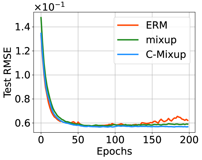
(a) : Test Loss

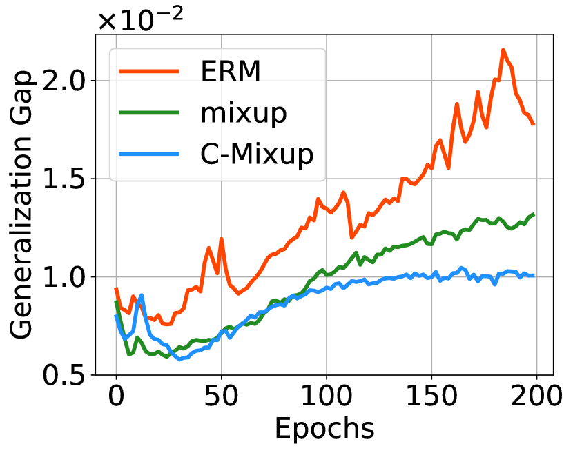
(b) : Generalization Gap

Figure 7: Additional overfitting analysis of electricity

C.4 Full Results

In Table 9, we report the full results of in-distribution generalization.

Table 9: Full results of in-distribution generalization. We compute the mean and standard deviation for results of three seeds.

		Airfoil	NO2	Exchange-Rate	Electricity	Echo
RMSE	ERM	2.901 $\pm$ 0.067	0.537 $\pm$ 0.005	0.0236 $\pm$ 0.0031	0.0581 $\pm$ 0.0011	5.402 $\pm$ 0.024
	mixup	3.730 $\pm$ 0.190	0.528 $\pm$ 0.005	0.0239 $\pm$ 0.0027	0.0585 $\pm$ 0.0004	5.393 $\pm$ 0.040
	Mani mixup	3.063 $\pm$ 0.113	0.522 $\pm$ 0.008	0.0242 $\pm$ 0.0043	0.0583 $\pm$ 0.0004	5.482 $\pm$ 0.066
	k-Mixup	2.938 $\pm$ 0.150	0.519 $\pm$ 0.005	0.0236 $\pm$ 0.0029	0.0575 $\pm$ 0.0002	5.518 $\pm$ 0.034
	Local Mixup	3.703 $\pm$ 0.151	0.517 $\pm$ 0.004	0.0236 $\pm$ 0.0024	0.0582 $\pm$ 0.0004	5.652 $\pm$ 0.043
	MixRL	3.614 $\pm$ 0.293	0.527 $\pm$ 0.003	0.0238 $\pm$ 0.0037	0.0585 $\pm$ 0.0006	5.618 $\pm$ 0.071
	C-Mixup (Ours)	2.717 $\pm$ 0.067	0.509 $\pm$ 0.006	0.0203 $\pm$ 0.0011	0.0570 $\pm$ 0.0006	5.177 $\pm$ 0.036
MAPE	ERM	1.753 $\pm$ 0.078%	13.615 $\pm$ 0.165%	2.423 $\pm$ 0.365%	13.861 $\pm$ 0.152%	8.700 $\pm$ 0.015%
	mixup	2.327 $\pm$ 0.159%	13.534 $\pm$ 0.125%	2.441 $\pm$ 0.286%	14.306 $\pm$ 0.048%	8.838 $\pm$ 0.108%
	Mani mixup	1.842 $\pm$ 0.114%	13.382 $\pm$ 0.360%	2.475 $\pm$ 0.346%	14.556 $\pm$ 0.057%	8.955 $\pm$ 0.082%
	k-Mixup	1.769 $\pm$ 0.035%	13.173 $\pm$ 0.139%	2.403 $\pm$ 0.311%	14.134 $\pm$ 0.134%	9.206 $\pm$ 0.117%
	Local Mixup	2.290 $\pm$ 0.101%	13.202 $\pm$ 0.176%	2.341 $\pm$ 0.229%	14.245 $\pm$ 0.152%	9.313 $\pm$ 0.115%
	MixRL	2.163 $\pm$ 0.219%	13.298 $\pm$ 0.182%	2.397 $\pm$ 0.296%	14.417 $\pm$ 0.203%	9.165 $\pm$ 0.134%
	C-Mixup (Ours)	1.610 $\pm$ 0.085%	12.998 $\pm$ 0.271%	2.041 $\pm$ 0.134%	13.372 $\pm$ 0.106%	8.435 $\pm$ 0.089%

Appendix D Additional Experiments of Task Generalization

D.1 Detailed Dataset Description

ShapeNet1D. We adopt the same preprocessing strategy to preprocess the ShapeNet1D dataset [18]. The ShapeNet1D dataset contains 27 categories with 60 objects per category. For each category, we randomly select 50 objects for meta-training and the rest ones are used for meta-testing. The model takes a $128\times 128$ grey-scale image as the input, and the label is normalized to $[0,10]$.

PASCAL3D. In PASCAL3D, we follow [79] to preprocess the dataset, where 50 and 15 categories are used for meta-training and meta-testing, respectively. The input image size and output label scale are same as ShapeNet1D.

D.2 Hyperparameters.

We list the hyperparameters used in the experiments of ShapeNet1D and PASCAL3D in Table 10.

Table 10: Hyperparameters of task generalization experiments.

Hyperparameters	ShapeNet1D	PASCAL3D
outer-loop learning rate	0.0005	0.001
inner-loop learning rate	0.002	0.01
# of inner-loop updates	5	5
$\alpha$ in Beta Dist.	0.5	0.5
batch size	10	10
support/query shot	15	15
max. iterations	15,000	15,000

Appendix E Additional Experiments of Out-of-Distribution Robustness

E.1 Detailed Dataset Description

We provide detailed descriptions for datasets that are used in the experiments of out-of-distribution robustness.

Table 11: Spurious correlation analysis in RCF-MNIST. We list the test performance w/ and w/o distribution shifts.

	w/o shift	w/ shift
RMSE $\downarrow$	0.111	0.162

RCF-MNIST. The prefix "RCF" of RCF-MNIST means "Rotated-Colored-Fashion". To construct RCF-MNIST, assume the normalized RGB vector of red and blue is $[1,0,0]$ and $[0,0,1]$ and the normalized angle of rotation (i.e., label) for one image is $g\in[0,1]$. In training set, we color 80% images with RGB value $[g,0,1-g]$ and the rest images are colored with $[1-g,0,g]$. Hence, the color information is strongly spuriously correlated with the label in the training set. In test set, we reverse spurious correlations to simulate distribution shift, where $80\%$ and $20\%$ images are colored with RGB values $[1-g,0,g]$ and $[g,0,1-g]$, respectively. We further verify that the spurious correlation between color and label affects the performance. Here, we compare the performance of same test set with or without distribution shift. The results are reported in Table 11, where we observe that the subpopulation shift caused by spurious correlation does hurt the performance as expected.

PovertyMap is included in the WILDS benchmark [34], which contains satellite images from 23 African countries that can be used to predict the village-level real-valued asset wealth index. The input is a $224\times 224$ multispectral LandSat satellite image with 8 channels, and the label is the real-valued asset wealth index. The domains of the images consist the country, urban and rural area information. This dataset includes 5 different cross validation folds, and all countries in these splits are disjoint to support the out-of-distribution setting. All experimental settings follow Koh et al. [34].

Communities And Crimes (Crime) is a tabular dataset combining socio-economic data from the 1990 US Census, law enforcement data from the 1990 US LEMAS survey, and crime data from the 1995 FBI UCR. The input features include 122 attributes that have some plausible connection to crime, such as the median family income and percent of officers assigned to drug units. The label attribute to be predicted is per capita violent crimes, which covers violent crimes including murder, rape, robbery, assault and so on. All numeric features are normalized into the decimal range $0.00\sim 1.00$ by equal-interval binning method, and the missing values are filled with the average values of the corresponding attributes. State identifications are used as the domain information, resulting to 46 domains in total. We split the dataset into training, validation and test sets with size 1,390, 231 and 373, while they contain 31, 6 and 9 disjoint domains, respectively.

SkillCraft. SkillCraft is a UCI tabular dataset [6] originated from a study that used video game telemetry data from real-time strategy (RTS) games to explore the development of expertise. Input x contains 17 player-related parameters in the game, such as the Cognition-Action-cycle variables and the Hotkey Usage variables. And the action latency in the game was considered as the label y. Missing data are filled by mean padding on each attribute. We use "League Index", which correspond to different levels of competitors, to be the identifier of domain. The dataset is split into training, validation and test sets with size $1878$, $806$, $711$ and disjoint domain number $4$, $1$, $3$, respectively.

Drug-target Interactions (DTI). Drug-target Interactions dataset  [28] originated aims to predict the binding activity score between each small molecule and the corresponding target protein. The input features contain both drug and target protein information, which are represented by one-hot vectors. The output label is the binding activity score. The training and validation set are selected from 2013-2018, and test set is drawn from 2019-2020. We regard "Year" as the domain information.

E.2 Hyperparameters

We list the hyperparameters for the experiments of out-of-distribution robustness in Table 12.

Table 12: Hyperparameter settings for the experiments of out-of-distribution robustness.

Dataset	RCF-MNIST	PovertyMap	Crime	SkillCraft	DTI
Learning rate	7e-5	1e-3	1e-3	1e-2	5e-5
Weight decay	0	0	0	0	0
Scheduler	n/a	StepLR	n/a	n/a	n/a
Batch size	64	64	16	32	64
Type of mixup	ManiMix	CutMix	ManiMix	mixup	ManiMix
Architecture	ResNet-18	ResNet-50	FCN3	FCN3	DeepDTA
Optimizer	Adam	Adam	Adam	Adam	Adam
Maximum Epoch	30	50	200	100	20
Bandwidth $\sigma$	0.2	0.5	1.0	5e-4	21.0
$\alpha$ in Beta Dist.	2.0	0.5	2.0	2.0	2.0

E.3 Full Results

In Table 13, we report the full results of out-of-distribution robustness.

Table 13: Full results of out-of-distribution robustness. The standard deviations are calculated by 5-fold data split in PovertyMap [34], or over 3 seeds in other datasets.

	RCF-MNIST (RMSE)	PovertyMap ($R$)		Crime (RMSE)
	Avg. $\downarrow$	Avg. $\uparrow$	Worst $\uparrow$	Avg. $\downarrow$	Worst $\downarrow$
ERM	0.162 $\pm$ 0.003	0.80 $\pm$ 0.04	0.50 $\pm$ 0.07	0.134 $\pm$ 0.003	0.173 $\pm$ 0.009
IRM	0.153 $\pm$ 0.003	0.77 $\pm$ 0.05	0.43 $\pm$ 0.07	0.127 $\pm$ 0.001	0.155 $\pm$ 0.003
IB-IRM	0.167 $\pm$ 0.003	0.78 $\pm$ 0.05	0.40 $\pm$ 0.05	0.127 $\pm$ 0.002	0.153 $\pm$ 0.004
V-REx	0.154 $\pm$ 0.011	0.83 $\pm$ 0.02	0.48 $\pm$ 0.03	0.129 $\pm$ 0.005	0.157 $\pm$ 0.007
CORAL	0.163 $\pm$ 0.016	0.78 $\pm$ 0.05	0.44 $\pm$ 0.06	0.133 $\pm$ 0.007	0.166 $\pm$ 0.015
GroupDRO	0.232 $\pm$ 0.016	0.75 $\pm$ 0.07	0.39 $\pm$ 0.06	0.138 $\pm$ 0.005	0.168 $\pm$ 0.009
Fish	0.263 $\pm$ 0.017	0.80 $\pm$ 0.02	0.30 $\pm$ 0.01	0.128 $\pm$ 0.000	0.152 $\pm$ 0.001
mixup	0.176 $\pm$ 0.003	0.81 $\pm$ 0.04	0.46 $\pm$ 0.03	0.128 $\pm$ 0.002	0.154 $\pm$ 0.001
Ours	0.146 $\pm$ 0.005	0.81 $\pm$ 0.03	0.53 $\pm$ 0.07	0.123 $\pm$ 0.000	0.146 $\pm$ 0.002
	n/a	SkillCraft (RMSE)		DTI ($R$)
	n/a	Avg. $\downarrow$	Worst $\downarrow$	Avg. $\uparrow$	Worst $\uparrow$
ERM	n/a	5.887 $\pm$ 0.362	10.182 $\pm$ 1.745	0.464 $\pm$ 0.014	0.429 $\pm$ 0.004
IRM	n/a	5.937 $\pm$ 0.254	7.849 $\pm$ 0.371	0.478 $\pm$ 0.007	0.432 $\pm$ 0.003
IB-IRM	n/a	6.055 $\pm$ 0.503	7.650 $\pm$ 0.653	0.479 $\pm$ 0.009	0.435 $\pm$ 0.007
V-REx	n/a	6.059 $\pm$ 0.429	7.444 $\pm$ 0.494	0.485 $\pm$ 0.009	0.435 $\pm$ 0.004
CORAL	n/a	6.353 $\pm$ 0.102	8.272 $\pm$ 0.436	0.483 $\pm$ 0.010	0.432 $\pm$ 0.005
GroupDRO	n/a	6.155 $\pm$ 0.537	8.131 $\pm$ 0.608	0.442 $\pm$ 0.043	0.407 $\pm$ 0.039
Fish	n/a	6.356 $\pm$ 0.201	8.676 $\pm$ 1.159	0.470 $\pm$ 0.022	0.443 $\pm$ 0.010
mixup	n/a	5.764 $\pm$ 0.618	9.206 $\pm$ 0.878	0.465 $\pm$ 0.004	0.437 $\pm$ 0.016
Ours	n/a	5.201 $\pm$ 0.059	7.362 $\pm$ 0.244	0.498 $\pm$ 0.008	0.458 $\pm$ 0.004

Appendix F Additional Analysis of C-Mixup

F.1 Additional Compatibility Analysis

In Table 14, we report the full results of compatibility analysis. Here, the performances on ERM, mixup, mixup+C-Mixup are also reported for comparison. In addition to the compatibility of C-Mixup, we also observe that some powerful inter-class mixup policies (e.g., PuzzleMix) improve the performance on part of regression tasks, e.g., RCF-MNIST. However, these approaches may also yield worse performances than ERM in other datasets, e.g., PovertyMap. Nevertheless, integrating C-Mixup on these mixup-based variants performs better than their vanilla versions, showing the compatibility and complementarity of C-Mixup to the existing mixup-based approaches in regression.

Table 14: Full results (performance with standard deviation) of compatibility analysis.

Model		RCF-MNIST	PovertyMap
		RMSE $\downarrow$	Worst $R$ $\uparrow$
ERM		0.162 $\pm$ 0.003	0.50 $\pm$ 0.07
mixup		0.176 $\pm$ 0.003	n/a
	+C-Mixup	0.146 $\pm$ 0.005	n/a
CutMix		0.194 $\pm$ 0.010	0.46 $\pm$ 0.03
	+C-Mixup	0.186 $\pm$ 0.013	0.53 $\pm$ 0.07
PuzzleMix		0.159 $\pm$ 0.004	0.47 $\pm$ 0.03
	+C-Mixup	0.150 $\pm$ 0.012	0.50 $\pm$ 0.04
AutoMix		0.152 $\pm$ 0.021	0.49 $\pm$ 0.07
	+C-Mixup	0.146 $\pm$ 0.009	0.53 $\pm$ 0.07

F.2 Distance Metrics

In this section, we first discuss how to calculate the representation distance $d(h_{i},h_{j})$. Then, we provide complete analysis of distance metrics.

Measuring Representation Distance. In this paper, we adopt a two-stage training process for each iteration. In the first stage, we feed the data into the current backbone and get hidden representations $h$, which is used to calculate the example distance, i.e., $d(h_{i},h_{j})$. In the second stage, we apply C-Mixup with representation distance.

Complete Analysis of Distance Metrics We report full results of the analysis of distance metrics in Table 15. In addition to the existing analysis, we conduct one analysis by changing how to calculate the distance between low-dimensional hidden representations, where we compare the Euclidean distance and the cosine distance. We observe that C-Mixup performs better than using both Euclidean and cosine distances to measure the similarity between low-dimensional representations, corroborating the effectiveness of C-Mixup.

Table 15: Full results (performance with standard deviation) of different distance metrics.

Model	Exchange-Rate	ShapeNet1D	DTI
	RMSE $\downarrow$	MSE $\downarrow$	Avg. $R$ $\uparrow$
ERM/MAML	0.0236 $\pm$ 0.0031	4.698 $\pm$ 0.079	0.464 $\pm$ 0.014
mixup/MetaMix	0.0239 $\pm$ 0.0027	4.275 $\pm$ 0.082	0.465 $\pm$ 0.004
$d(x_{i},x_{j})$	0.0212 $\pm$ 0.0014	4.539 $\pm$ 0.082	0.478 $\pm$ 0.003
$d(x_{i}\oplus y_{i},x_{j}\oplus y_{j})$	0.0212 $\pm$ 0.0009	4.395 $\pm$ 0.085	0.484 $\pm$ 0.002
$d(h_{i},h_{j})$ (Euclidean distance)	0.0213 $\pm$ 0.0006	4.202 $\pm$ 0.078	0.483 $\pm$ 0.001
$d(h_{i},h_{j})$ (Cosine distance)	0.0209 $\pm$ 0.0012	4.411 $\pm$ 0.081	0.477 $\pm$ 0.004
$d(h_{i}\oplus y_{i},h_{j}\oplus y_{j})$	0.0208 $\pm$ 0.0016	4.176 $\pm$ 0.077	0.487 $\pm$ 0.001
$d(y_{i},y_{j})$ (C-Mixup)	0.0203 $\pm$ 0.0011	4.024 $\pm$ 0.081	0.498 $\pm$ 0.008

F.3 Additional Hyperparameter Sensitivity

In this section, we first provide more experiments for bandwidth analysis. Then, we conduct experiments to show the effect of hyperparameter $\alpha$ in Beta distribution, i.e., $\mathrm{Beta}(\alpha,\alpha)$.

F.3.1 Additional Bandwidth Analysis

We illustrate the bandwidth analysis for additional four datasets in Figure 8, including Airfoil, NO2, PovertyMap, SkillCraft. The results corroborate our finding in the main paper that C-Mixup yields a good model in a relative wide range of bandwidth, reducing the efforts to tune the bandwidth $\sigma$ for every specific dataset.

According to our empirical results, we conclude that roughly tuning the bandwidth in the range [0.01, 0.1, 1, 10, 100] is sufficient to get a relatively satisfying performance. To get the optimal bandwidth, we suggest to perform grid search.

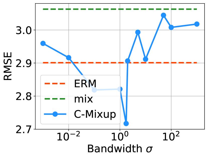
(a) : Airfoil

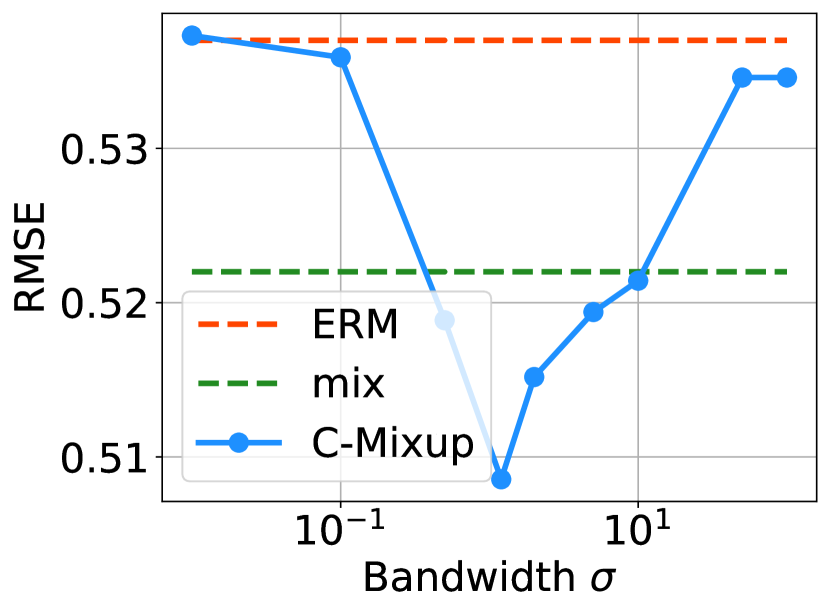
(b) : NO2

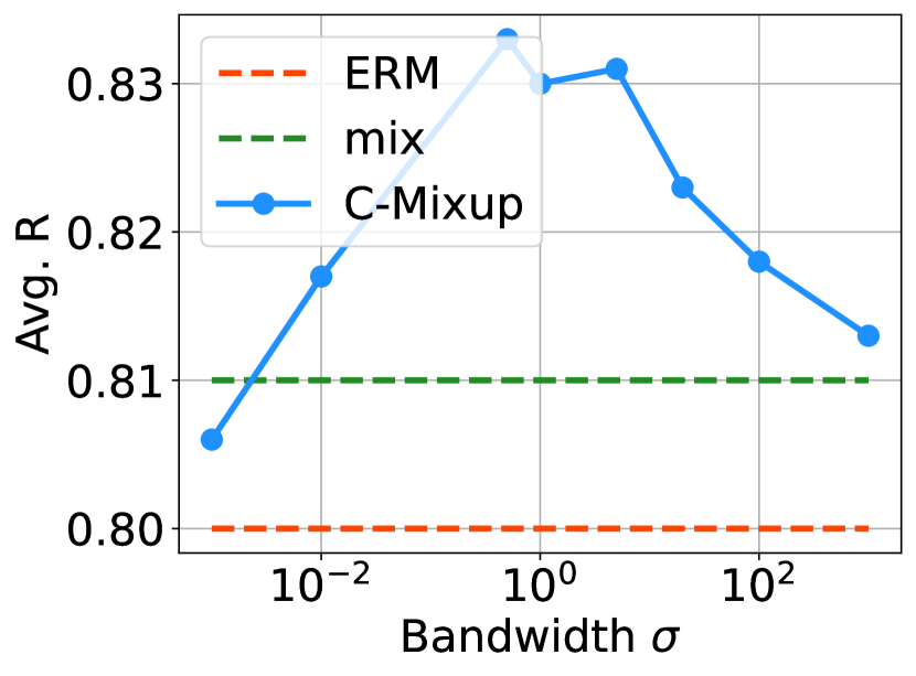
(c) : PovertyMap

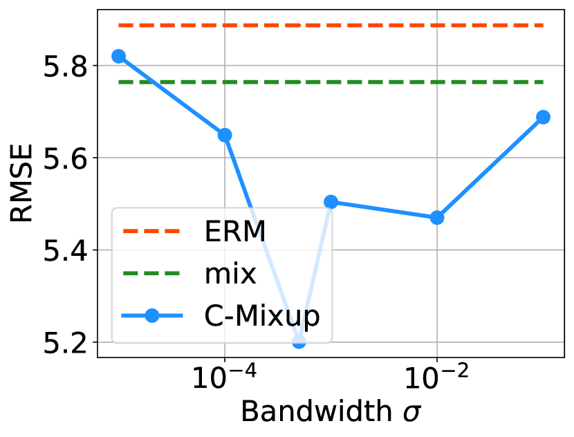
(d) : SkillCraft

Figure 8: Additional robustness analysis of bandwidth

F.3.2 Effect of Shape Parameter $\alpha$ in Beta Distribution

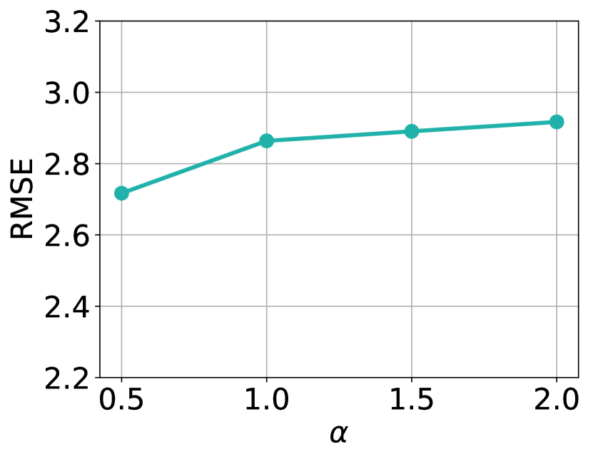
(a) : Airfoil

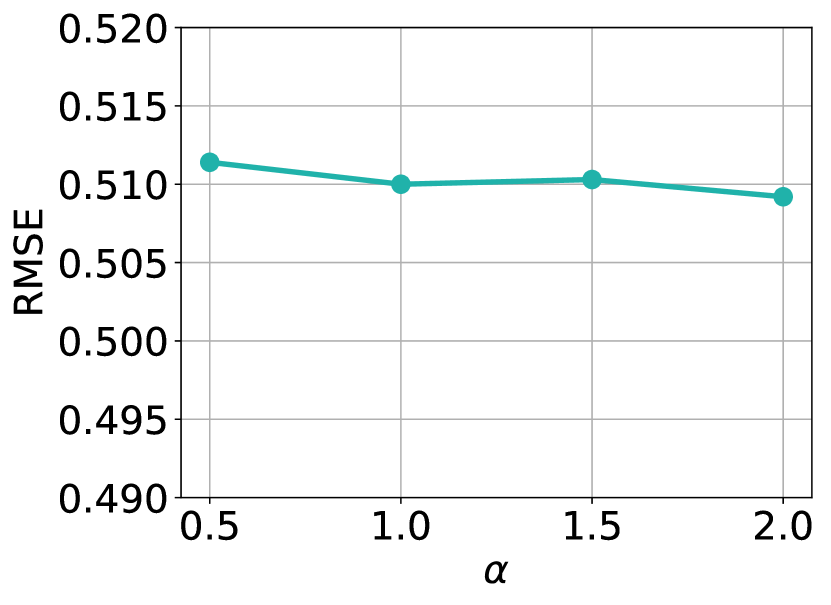
(b) : NO2

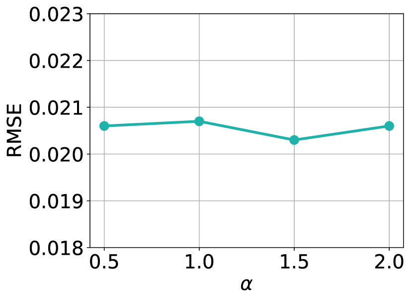
(c) : Exchange-Rate

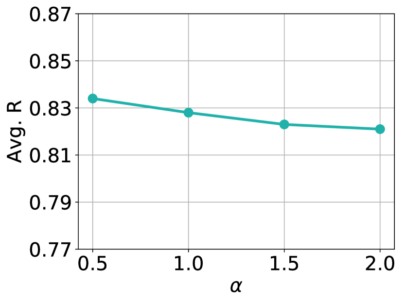
(d) : PovertyMap

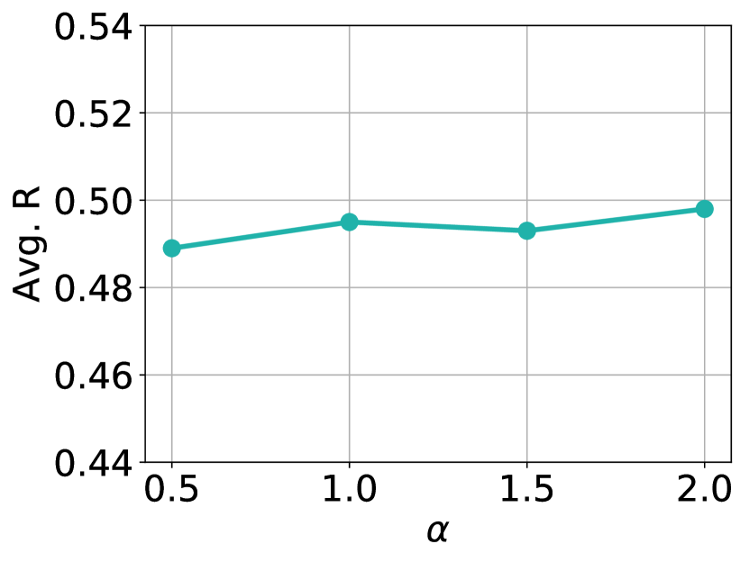
(e) : DTI

Figure 9: Robustness analysis of $\alpha$ in Beta distribution

Finally, we analyze the effect of shape parameter $\alpha$ in the Beta distribution. The results of five datasets are illustrated in Figure 9, including Airfoil, NO2, Exchange-Rate, PovertyMap, and DTI. We observe that the performance is relatively stable with the change of $\alpha$, indicating the robustness of C-Mixup to the shape of Beta distribution.

F.4 Robustness Analysis to Label Noise

We conduct experiments to investigate the robustness of C-Mixup to label noise. Specifically, we inject Gaussian noises into labels for all training examples. For each dataset, the noise is set as 30% of the standard deviation of the corresponding original labels, where adding noise significantly degrades the performance compared to that with clean data. The results and the corresponding noise distributions on three datasets – Exchange-Rate, ShapeNet1D, DTI are reported in Table 16. According to Table 16, C-Mixup still improves the performance over ERM and vanilla mixup, showing its robustness to label noise.

Table 16: Robustness analysis to label noise.

Model	Exchange-Rate	ShapeNet1D	DTI
	RMSE $\downarrow$	MSE $\downarrow$	Avg. $R$ $\uparrow$
Noise Type	$\mathcal{N}(0,1.18\times 10^{-3})$	$\mathcal{N}(0,0.874)$	$\mathcal{N}(0,7.59\times 10^{-3})$
ERM/MAML	0.0381 $\pm$ 0.0014	5.553 $\pm$ 0.098	0.334 $\pm$ 0.018
mixup/MetaMix	0.0375 $\pm$ 0.0017	5.329 $\pm$ 0.101	0.307 $\pm$ 0.021
C-Mixup	0.0360 $\pm$ 0.0013	5.185 $\pm$ 0.096	0.356 $\pm$ 0.013

References

- Ahuja et al. [2021] Kartik Ahuja, Ethan Caballero, Dinghuai Zhang, Yoshua Bengio, Ioannis Mitliagkas, and Irina Rish. Invariance principle meets information bottleneck for out-of-distribution generalization. 2021.
- Aldrin [2004] Magne Aldrin. Cmu statlib dataset, 2004. http://lib.stat.cmu.edu/datasets/, Last accessed on May. 22th, 2022.
- Antoniou et al. [2017] Antreas Antoniou, Amos Storkey, and Harrison Edwards. Data augmentation generative adversarial networks. arXiv preprint arXiv:1711.04340, 2017.
- Arjovsky et al. [2019] Martin Arjovsky, Léon Bottou, Ishaan Gulrajani, and David Lopez-Paz. Invariant risk minimization. arXiv preprint arXiv:1907.02893, 2019.
- Baena et al. [2022] Raphael Baena, Lucas Drumetz, and Vincent Gripon. Preventing manifold intrusion with locality: Local mixup. arXiv preprint arXiv:2201.04368, 2022.
- Blair et al. [2013] Mark Blair, Joe Thompson, Andrew Henrey, and Bill Chen. SkillCraft1 Master Table Dataset. UCI Machine Learning Repository, 2013.
- Bowles et al. [2018] Christopher Bowles, Liang Chen, Ricardo Guerrero, Paul Bentley, Roger Gunn, Alexander Hammers, David Alexander Dickie, Maria Valdés Hernández, Joanna Wardlaw, and Daniel Rueckert. Gan augmentation: Augmenting training data using generative adversarial networks. arXiv preprint arXiv:1810.10863, 2018.
- Brooks [2014] Pope D. & Marcolini Michael Brooks, Thomas. Airfoil Self-Noise. UCI Machine Learning Repository, 2014.
- Chen et al. [2022] Jie-Neng Chen, Shuyang Sun, Ju He, Philip HS Torr, Alan Yuille, and Song Bai. Transmix: Attend to mix for vision transformers. In Proceedings of the IEEE/CVF Conference on Computer Vision and Pattern Recognition, pages 12135–12144, 2022.
- Cubuk et al. [2019] Ekin D Cubuk, Barret Zoph, Dandelion Mane, Vijay Vasudevan, and Quoc V Le. Autoaugment: Learning augmentation strategies from data. In Proceedings of the IEEE/CVF Conference on Computer Vision and Pattern Recognition, pages 113–123, 2019.
- Cubuk et al. [2020] Ekin D Cubuk, Barret Zoph, Jonathon Shlens, and Quoc V Le. Randaugment: Practical automated data augmentation with a reduced search space. In Proceedings of the IEEE/CVF Conference on Computer Vision and Pattern Recognition Workshops, pages 702–703, 2020.
- DeVries and Taylor [2017] Terrance DeVries and Graham W Taylor. Improved regularization of convolutional neural networks with cutout. arXiv preprint arXiv:1708.04552, 2017.
- Dua and Graff [2017] Dheeru Dua and Casey Graff. UCI machine learning repository, 2017. URL http://archive.ics.uci.edu/ml.
- Finn and Levine [2017] Chelsea Finn and Sergey Levine. Meta-learning and universality: Deep representations and gradient descent can approximate any learning algorithm. arXiv preprint arXiv:1710.11622, 2017.
- Gal and Ghahramani [2016] Yarin Gal and Zoubin Ghahramani. Dropout as a bayesian approximation: Representing model uncertainty in deep learning. In ICML, pages 1050–1059, 2016.
- Ganin and Lempitsky [2015] Yaroslav Ganin and Victor Lempitsky. Unsupervised domain adaptation by backpropagation. In International conference on machine learning, pages 1180–1189. PMLR, 2015.
- Ganin et al. [2016] Yaroslav Ganin, Evgeniya Ustinova, Hana Ajakan, Pascal Germain, Hugo Larochelle, François Laviolette, Mario Marchand, and Victor Lempitsky. Domain-adversarial training of neural networks. The journal of machine learning research, 17(1):2096–2030, 2016.
- Gao et al. [2022] Ning Gao, Hanna Ziesche, Ngo Anh Vien, Michael Volpp, and Gerhard Neumann. What matters for meta-learning vision regression tasks? 2022.
- Ge et al. [2019] Rong Ge, Rohith Kuditipudi, Zhize Li, and Xiang Wang. Learning two-layer neural networks with symmetric inputs. In International Conference on Learning Representations, 2019.
- Greenewald et al. [2021] Kristjan Greenewald, Anming Gu, Mikhail Yurochkin, Justin Solomon, and Edward Chien. k-mixup regularization for deep learning via optimal transport. arXiv preprint arXiv:2106.02933, 2021.
- Guiroy et al. [2019] Simon Guiroy, Vikas Verma, and Christopher Pal. Towards understanding generalization in gradient-based meta-learning. arXiv preprint arXiv:1907.07287, 2019.
- Guo et al. [2019] Hongyu Guo, Yongyi Mao, and Richong Zhang. Mixup as locally linear out-of-manifold regularization. In Proceedings of the AAAI Conference on Artificial Intelligence, volume 33, pages 3714–3722, 2019.
- Guo et al. [2021] Ruocheng Guo, Pengchuan Zhang, Hao Liu, and Emre Kiciman. Out-of-distribution prediction with invariant risk minimization: The limitation and an effective fix. arXiv preprint arXiv:2101.07732, 2021.
- Hendrycks et al. [2019] Dan Hendrycks, Norman Mu, Ekin D Cubuk, Barret Zoph, Justin Gilmer, and Balaji Lakshminarayanan. Augmix: A simple data processing method to improve robustness and uncertainty. arXiv preprint arXiv:1912.02781, 2019.
- Hoerl and Kennard [1970] Arthur E. Hoerl and Robert W. Kennard. Ridge regression: Biased estimation for nonorthogonal problems. Technometrics, 12(1):55–67, 1970. doi: 10.1080/00401706.1970.10488634. URL https://www.tandfonline.com/doi/abs/10.1080/00401706.1970.10488634.
- Hong et al. [2021] Minui Hong, Jinwoo Choi, and Gunhee Kim. Stylemix: Separating content and style for enhanced data augmentation. In Proceedings of the IEEE/CVF Conference on Computer Vision and Pattern Recognition, pages 14862–14870, 2021.
- Horowitz [2009] Joel L Horowitz. Semiparametric and nonparametric methods in econometrics, volume 12. Springer, 2009.
- Huang et al. [2021] Kexin Huang, Tianfan Fu, Wenhao Gao, Yue Zhao, Yusuf Roohani, Jure Leskovec, Connor W Coley, Cao Xiao, Jimeng Sun, and Marinka Zitnik. Therapeutics data commons: Machine learning datasets and tasks for therapeutics. arXiv preprint arXiv:2102.09548, 2021.
- Hwang and Whang [2021] Seong-Hyeon Hwang and Steven Euijong Whang. Mixrl: Data mixing augmentation for regression using reinforcement learning. arXiv preprint arXiv:2106.03374, 2021.
- Jamal and Qi [2019] Muhammad Abdullah Jamal and Guo-Jun Qi. Task agnostic meta-learning for few-shot learning. In Proceedings of the IEEE/CVF Conference on Computer Vision and Pattern Recognition, pages 11719–11727, 2019.
- Khezeli et al. [2021] Kia Khezeli, Arno Blaas, Frank Soboczenski, Nicholas Chia, and John Kalantari. On invariance penalties for risk minimization. arXiv preprint arXiv:2106.09777, 2021.
- Kim et al. [2020] Jang-Hyun Kim, Wonho Choo, and Hyun Oh Song. Puzzle mix: Exploiting saliency and local statistics for optimal mixup. In International Conference on Machine Learning, pages 5275–5285. PMLR, 2020.
- Kim et al. [2021] Jang-Hyun Kim, Wonho Choo, Hosan Jeong, and Hyun Oh Song. Co-mixup: Saliency guided joint mixup with supermodular diversity. arXiv preprint arXiv:2102.03065, 2021.
- Koh et al. [2021] Pang Wei Koh, Shiori Sagawa, Sang Michael Xie, Marvin Zhang, Akshay Balsubramani, Weihua Hu, Michihiro Yasunaga, Richard Lanas Phillips, Irena Gao, Tony Lee, et al. Wilds: A benchmark of in-the-wild distribution shifts. In International Conference on Machine Learning, pages 5637–5664. PMLR, 2021.
- Kooperberg [1997] Charles Kooperberg. Statlib: an archive for statistical software, datasets, and information. The American Statistician, 51(1):98, 1997.
- Koyama and Yamaguchi [2020] Masanori Koyama and Shoichiro Yamaguchi. Out-of-distribution generalization with maximal invariant predictor. arXiv preprint arXiv:2008.01883, 2020.
- Krizhevsky et al. [2012] Alex Krizhevsky, Ilya Sutskever, and Geoffrey E Hinton. Imagenet classification with deep convolutional neural networks. In Annual Conference on Neural Information Processing Systems, pages 1097–1105, 2012.
- Krogh and Hertz [1992] Anders Krogh and John A Hertz. A simple weight decay can improve generalization. In NeurIPS, pages 950–957, 1992.
- Krueger et al. [2021] David Krueger, Ethan Caballero, Joern-Henrik Jacobsen, Amy Zhang, Jonathan Binas, Dinghuai Zhang, Remi Le Priol, and Aaron Courville. Out-of-distribution generalization via risk extrapolation (rex). In International Conference on Machine Learning, pages 5815–5826. PMLR, 2021.
- Lai et al. [2018] Guokun Lai, Wei-Cheng Chang, Yiming Yang, and Hanxiao Liu. Modeling long-and short-term temporal patterns with deep neural networks. In The 41st International ACM SIGIR Conference on Research & Development in Information Retrieval, pages 95–104, 2018.
- Li et al. [2018] Haoliang Li, Sinno Jialin Pan, Shiqi Wang, and Alex C Kot. Domain generalization with adversarial feature learning. In Proceedings of the IEEE Conference on Computer Vision and Pattern Recognition, pages 5400–5409, 2018.
- Li et al. [2022] Haoyang Li, Ziwei Zhang, Xin Wang, and Wenwu Zhu. Learning invariant graph representations for out-of-distribution generalization. In Advances in Neural Information Processing Systems, 2022.
- Lim et al. [2019] Sungbin Lim, Ildoo Kim, Taesup Kim, Chiheon Kim, and Sungwoong Kim. Fast autoaugment. Advances in Neural Information Processing Systems, 32, 2019.
- Liu et al. [2022a] Jihao Liu, Boxiao Liu, Hang Zhou, Hongsheng Li, and Yu Liu. Tokenmix: Rethinking image mixing for data augmentation in vision transformers. arXiv preprint arXiv:2207.08409, 2022a.
- Liu et al. [2022b] Zicheng Liu, Siyuan Li, Di Wu, Zhiyuan Chen, Lirong Wu, Jianzhu Guo, and Stan Z Li. Automix: Unveiling the power of mixup for stronger classifiers. In ECCV, 2022b.
- Long et al. [2015] Mingsheng Long, Yue Cao, Jianmin Wang, and Michael Jordan. Learning transferable features with deep adaptation networks. In International conference on machine learning, pages 97–105. PMLR, 2015.
- Lyu and Li [2019] Kaifeng Lyu and Jian Li. Gradient descent maximizes the margin of homogeneous neural networks. In International Conference on Learning Representations, 2019.
- Neyshabur [2017] Behnam Neyshabur. Implicit regularization in deep learning. arXiv preprint arXiv:1709.01953, 2017.
- Ni et al. [2021] Renkun Ni, Micah Goldblum, Amr Sharaf, Kezhi Kong, and Tom Goldstein. Data augmentation for meta-learning. ICML, 2021.
- Ouyang et al. [2020] David Ouyang, Bryan He, Amirata Ghorbani, Neal Yuan, Joseph Ebinger, Curtis P Langlotz, Paul A Heidenreich, Robert A Harrington, David H Liang, Euan A Ashley, et al. Video-based ai for beat-to-beat assessment of cardiac function. Nature, 580(7802):252–256, 2020.
- Öztürk et al. [2018] Hakime Öztürk, Arzucan Özgür, and Elif Ozkirimli. Deepdta: deep drug–target binding affinity prediction. Bioinformatics, 34(17):i821–i829, 2018.
- Park et al. [2022] Joonhyung Park, June Yong Yang, Jinwoo Shin, Sung Ju Hwang, and Eunho Yang. Saliency grafting: Innocuous attribution-guided mixup with calibrated label mixing. In Proceedings of the AAAI Conference on Artificial Intelligence, volume 36, pages 7957–7965, 2022.
- Powell et al. [1989] James L Powell, James H Stock, and Thomas M Stoker. Semiparametric estimation of index coefficients. Econometrica: Journal of the Econometric Society, pages 1403–1430, 1989.
- Raghu et al. [2020] Aniruddh Raghu, Maithra Raghu, Samy Bengio, and Oriol Vinyals. Rapid learning or feature reuse? towards understanding the effectiveness of maml. In International Conference on Learning Representations, 2020.
- Rajendran et al. [2020] Janarthanan Rajendran, Alex Irpan, and Eric Jang. Meta-learning requires meta-augmentation. In International Conference on Neural Information Processing Systems, 2020.
- Redmond [2009] Michael Redmond. Communities and Crime. UCI Machine Learning Repository, 2009.
- [57] Philippe Rigollet and Jan-Christian Hütter. High dimensional statistics.
- Sagawa et al. [2020] Shiori Sagawa, Pang Wei Koh, Tatsunori B Hashimoto, and Percy Liang. Distributionally robust neural networks for group shifts: On the importance of regularization for worst-case generalization. In ICLR, 2020.
- Shi et al. [2021] Yuge Shi, Jeffrey Seely, Philip HS Torr, N Siddharth, Awni Hannun, Nicolas Usunier, and Gabriel Synnaeve. Gradient matching for domain generalization. arXiv preprint arXiv:2104.09937, 2021.
- Srivastava et al. [2014] Nitish Srivastava, Geoffrey Hinton, Alex Krizhevsky, Ilya Sutskever, and Ruslan Salakhutdinov. Dropout: a simple way to prevent neural networks from overfitting. JMLR, 15(1):1929–1958, 2014.
- Stein et al. [2004] Charles Stein, Persi Diaconis, Susan Holmes, Gesine Reinert, et al. Use of exchangeable pairs in the analysis of simulations. In Stein’s Method, volume 46, pages 1–26. Institute of Mathematical Statistics, 2004.
- Tripuraneni et al. [2021] Nilesh Tripuraneni, Chi Jin, and Michael Jordan. Provable meta-learning of linear representations. In International Conference on Machine Learning, pages 10434–10443. PMLR, 2021.
- Tseng et al. [2020] Hung-Yu Tseng, Yi-Wen Chen, Yi-Hsuan Tsai, Sifei Liu, Yen-Yu Lin, and Ming-Hsuan Yang. Regularizing meta-learning via gradient dropout. In Proceedings of the Asian Conference on Computer Vision, 2020.
- Tsybakov [2004] Alexandre B Tsybakov. Introduction to nonparametric estimation, 2009. URL https://doi. org/10.1007/b13794. Revised and extended from the, 9(10), 2004.
- Tzeng et al. [2014] Eric Tzeng, Judy Hoffman, Ning Zhang, Kate Saenko, and Trevor Darrell. Deep domain confusion: Maximizing for domain invariance. arXiv preprint arXiv:1412.3474, 2014.
- Uddin et al. [2020] AFM Uddin, Mst Monira, Wheemyung Shin, TaeChoong Chung, Sung-Ho Bae, et al. Saliencymix: A saliency guided data augmentation strategy for better regularization. arXiv preprint arXiv:2006.01791, 2020.
- Venkataramanan et al. [2022] Shashanka Venkataramanan, Ewa Kijak, Laurent Amsaleg, and Yannis Avrithis. Alignmixup: Improving representations by interpolating aligned features. In Proceedings of the IEEE/CVF Conference on Computer Vision and Pattern Recognition, pages 19174–19183, 2022.
- Verma et al. [2019] Vikas Verma, Alex Lamb, Christopher Beckham, Amir Najafi, Ioannis Mitliagkas, David Lopez-Paz, and Yoshua Bengio. Manifold mixup: Better representations by interpolating hidden states. In International Conference on Machine Learning, pages 6438–6447. PMLR, 2019.
- [69] Roman Vershynin. High-dimensional probability: An introduction with application in data science.
- Wang et al. [2020] Kaixin Wang, Bingyi Kang, Jie Shao, and Jiashi Feng. Improving generalization in reinforcement learning with mixture regularization. Advances in Neural Information Processing Systems, 33:7968–7978, 2020.
- Xiang et al. [2014] Yu Xiang, Roozbeh Mottaghi, and Silvio Savarese. Beyond pascal: A benchmark for 3d object detection in the wild. In WACV, pages 75–82. IEEE, 2014.
- Xu et al. [2020] Minghao Xu, Jian Zhang, Bingbing Ni, Teng Li, Chengjie Wang, Qi Tian, and Wenjun Zhang. Adversarial domain adaptation with domain mixup. In Proceedings of the AAAI Conference on Artificial Intelligence, volume 34, pages 6502–6509, 2020.
- Yang et al. [2017] Zhuoran Yang, Krishnakumar Balasubramanian, and Han Liu. High-dimensional non-gaussian single index models via thresholded score function estimation. In International conference on machine learning, pages 3851–3860. PMLR, 2017.
- Yao et al. [2021] Huaxiu Yao, Longkai Huang, Linjun Zhang, Ying Wei, Li Tian, James Zou, Junzhou Huang, and Zhenhui Li. Improving generalization in meta-learning via task augmentation. In Proceeding of the Thirty-eighth International Conference on Machine Learning, 2021.
- Yao et al. [2022a] Huaxiu Yao, Caroline Choi, Bochuan Cao, Yoonho Lee, Pang Wei Koh, and Chelsea Finn. Wild-time: A benchmark of in-the-wild distribution shift over time. In Thirty-sixth Conference on Neural Information Processing Systems Datasets and Benchmarks Track, 2022a.
- Yao et al. [2022b] Huaxiu Yao, Yu Wang, Sai Li, Linjun Zhang, Weixin Liang, James Zou, and Chelsea Finn. Improving out-of-distribution robustness via selective augmentation. arXiv preprint arXiv:2201.00299, 2022b.
- Yao et al. [2022c] Huaxiu Yao, Linjun Zhang, and Chelsea Finn. Meta-learning with fewer tasks through task interpolation. In Proceeding of the 10th International Conference on Learning Representations, 2022c.
- Yeh et al. [2020] Christopher Yeh, Anthony Perez, Anne Driscoll, George Azzari, Zhongyi Tang, David Lobell, Stefano Ermon, and Marshall Burke. Using publicly available satellite imagery and deep learning to understand economic well-being in africa. Nature Communications, 2020.
- Yin et al. [2020] Mingzhang Yin, George Tucker, Mingyuan Zhou, Sergey Levine, and Chelsea Finn. Meta-learning without memorization. In International Conference on Learning Representations, 2020.
- Yue et al. [2019] Xiangyu Yue, Yang Zhang, Sicheng Zhao, Alberto Sangiovanni-Vincentelli, Kurt Keutzer, and Boqing Gong. Domain randomization and pyramid consistency: Simulation-to-real generalization without accessing target domain data. In Proceedings of the IEEE/CVF International Conference on Computer Vision, pages 2100–2110, 2019.
- Yun et al. [2019] Sangdoo Yun, Dongyoon Han, Seong Joon Oh, Sanghyuk Chun, Junsuk Choe, and Youngjoon Yoo. Cutmix: Regularization strategy to train strong classifiers with localizable features. In Proceedings of the IEEE/CVF International Conference on Computer Vision, pages 6023–6032, 2019.
- Zhang et al. [2018] Hongyi Zhang, Moustapha Cisse, Yann N Dauphin, and David Lopez-Paz. mixup: Beyond empirical risk minimization. 2018.
- Zhang et al. [2021] Linjun Zhang, Zhun Deng, Kenji Kawaguchi, Amirata Ghorbani, and James Zou. How does mixup help with robustness and generalization? In ICLR, 2021.
- Zhang et al. [2020] Rongzhi Zhang, Yue Yu, and Chao Zhang. Seqmix: Augmenting active sequence labeling via sequence mixup. arXiv preprint arXiv:2010.02322, 2020.
- Zhou et al. [2022] Allan Zhou, Fahim Tajwar, Alexander Robey, Tom Knowles, George J Pappas, Hamed Hassani, and Chelsea Finn. Do deep networks transfer invariances across classes? arXiv preprint arXiv:2203.09739, 2022.
- Zhou et al. [2020] Kaiyang Zhou, Yongxin Yang, Timothy Hospedales, and Tao Xiang. Deep domain-adversarial image generation for domain generalisation. In Proceedings of the AAAI Conference on Artificial Intelligence, volume 34, pages 13025–13032, 2020.
- Zhu et al. [2020] Jianchao Zhu, Liangliang Shi, Junchi Yan, and Hongyuan Zha. Automix: Mixup networks for sample interpolation via cooperative barycenter learning. In European Conference on Computer Vision, pages 633–649. Springer, 2020.
- Zoph et al. [2020] Barret Zoph, Ekin D Cubuk, Golnaz Ghiasi, Tsung-Yi Lin, Jonathon Shlens, and Quoc V Le. Learning data augmentation strategies for object detection. In European conference on computer vision, pages 566–583. Springer, 2020.