CNOT-Efficient Circuits for Arbitrary Rank Many-Body Fermionic and Qubit Excitations

Abstract

Efficient quantum circuits are necessary for realizing quantum algorithms on noisy intermediate-scale quantum devices. Fermionic excitations entering unitary coupled-cluster (UCC) ansätze give rise to quantum circuits containing CNOT “staircases” whose number scales exponentially with the excitation rank. Recently, Yordanov et al. [Phys. Rev. A 102, 062612 (2020); Commun. Phys. 4, 228 (2021)] constructed CNOT-efficient quantum circuits for both fermionic- (FEB) and qubit-excitation-based (QEB) singles and doubles and illustrated their usefulness in adaptive derivative-assembled pseudo-Trotterized variational quantum eigensolver (ADAPT-VQE) simulations. In this work, we extend these CNOT-efficient quantum circuits to arbitrary excitation ranks. To illustrate the benefits of these compact FEB and QEB quantum circuits, we perform numerical simulations using the recently developed selected projective quantum eigensolver (SPQE) approach, which relies on an adaptive UCC ansatz built from arbitrary-order particle–hole excitation operators. We show that both FEB- and QEB-SPQE decrease the number of CNOT gates compared to traditional SPQE by factors as large as 15. At the same time, QEB-SPQE requires, in general, more ansatz parameters than FEB-SPQE, in particular those corresponding to higher-than-double excitations, resulting in quantum circuits with larger CNOT counts. Although ADAPT-VQE generates quantum circuits with fewer CNOTs than SPQE, SPQE requires orders of magnitude less residual element evaluations than gradient element evaluations in ADAPT-VQE.

I Introduction

Since their inception more than 40 years ago, quantum computers have been anticipated to perform certain computational tasks more efficiently than a classical machine [1, 2, 3, 4]. An area where quantum computers can potentially have an advantage over their classical counterparts is the simulation of quantum many-body systems, such as those encountered in chemistry, condensed matter physics, and materials science. One of the main reasons behind this speed-up is the ability of quantum devices to represent highly entangled many-body states with a number of qubits proportional to the system size, a manifestation of Feynman’s rule of simulation [3].

Unfortunately, the reality is more complicated and physical realizations of quantum devices are plagued by various kinds of errors, such as imperfections of qubits, limited connectivity among qubits, decoherence of quantum states, readout errors, and errors in implementing quantum gates [5]. These issues could be remedied by fault-tolerant quantum computers, utilizing many physical qubits to encode a single logical one [6]. Nevertheless, scaling up the size of quantum devices is nothing short of an “experimenter’s nightmare” [7].

The technological advances aimed at improving the error rates of present noisy intermediate-scale quantum (NISQ) devices [5] have been accompanied by developments in the field of quantum algorithms [8]. To fully utilize current quantum hardware, hybrid quantum–classical approaches have been developed that require shallower circuits than pure quantum algorithms, e.g., quantum phase estimation [9, 10, 11]. The first such hybrid approach was the variational quantum eigensolver (VQE) [12, 13, 14, 15, 16], where the lowest eigenvalue of a Hamiltonian is estimated by minimizing its expectation value with respect to a parameterized trial state. In the projective quantum eigensolver (PQE) [17], the optimization procedure relies on residuals, namely, projections of the Schrödinger equation onto a linearly independent basis. The contracted quantum eigensolver (CQE) [18] is another approach using residuals, this time of the two-particle anti-Hermitian contracted Schrödinger equation [19]. In applications to electronic structure, one typically employs fermionic ansätze. In the case of VQE and PQE, in particular, the chemically inspired ansätze based on the unitary extension [20, 21, 22, 23, 24, 25, 26, 27, 28, 29, 30, 31, 32] of coupled-cluster (CC) theory [33, 34, 35, 36, 37, 38] (UCC) have been most popular. Recently, ansätze based on qubit excitations have been explored in the context of VQE [39, 40, 41, 42, 43, 44] and CQE [45, 46]. Such algorithms are potentially more computationally frugal since qubit excitations are native to quantum computers.

To further reduce the computational resources required by hybrid algorithms, extensions have been proposed that rely on iteratively constructed rather than fixed ansätze [47, 43, 42, 40, 17, 18, 45, 46, 48]. This additional flexibility results in a substantial reduction in the number of parameters needed to achieve a given accuracy in the computed energies, giving rise to shallower quantum circuits. In the popular adaptive derivative-assembled pseudo-Trotterized (ADAPT) VQE method [47], for example, one typically builds the ansatz one operator at a time from a pool containing single and double particle–hole excitation operators or their generalized variants [49, 50]. To allow ADAPT-VQE to converge to the exact, full configuration interaction (FCI), solution, a given excitation operator maybe be added to the ansatz multiple times, albeit with a different excitation amplitude. In contrast to ADAPT-VQE, the selected PQE (SPQE) approach [17] expands the ansatz by selecting a batch of operators from a complete pool of particle–hole excitations, including up to $N$-tuples where $N$ is the number of correlated electrons. In SPQE, the operator pool is allowed to “drain”, i.e., once an operator is selected to be appended to the ansatz, it is removed from the pool.

Despite the success of adaptive approaches, they generally still require a substantial number of two-qubit CNOT gates that is typically greater than that of the single-qubit ones. The fact that physical implementations of two-qubit gates are characterized by errors that are typically one order of magnitude larger than those associated with their single-qubit analogs (see, e.g., Ref. [51]) implies that CNOTs dominate the overall gate error. Consequently, to facilitate the experimental realization of quantum algorithms, it is crucial to reduce the CNOT count without introducing drastic approximations that adversely affect accuracies.

Recently, Yordanov et al. constructed the most CNOT-efficient quantum circuits to date representing single and double qubit excitations. Their qubit-excitation-based (QEB) approach reduced the CNOT count by 50% in the case of qubit singles and 73% for qubit doubles. These impressive reductions were attained without sacrificing accuracy, since the QEB quantum circuits are equivalent to their conventional counterparts. Yordanov et al. also extended their approach to fermionic excitations by making suitable modifications to their QEB quantum circuits. The performance of the fermionic-excitation-based (FEB) and QEB variants of ADAPT-VQE was recently examined [42]. It was demonstrated that QEB-ADAPT-VQE is almost as accurate as its FEB counterpart while requiring fewer CNOTs. In addition, QEB-ADAPT-VQE was shown to yield more compact ansätze than the qubit-ADAPT-VQE scheme of Ref. [43] when higher accuracy is desired.

Encouraged by the substantial reduction in CNOT count for single and double excitations, in this work we extend the CNOT-efficient quantum circuits of Yordanov et al. [41] to the $n$-body case. To illustrate their benefits, we implement and benchmark the FEB and QEB versions of the SPQE approach. In particular, we perform classical numerical simulations for the symmetric dissociations of $\text{BeH}_{2}$ (linear) and $\text{H}_{6}$ (linear, ring) and for the insertion of the Be atom into $\text{H}_{2}$. To demonstrate the savings in the CNOT count, we begin by comparing the FEB- and QEB-SPQE schemes with their traditional fermionic and qubit counterparts. We then proceed to the determination of the SPQE flavor that offers the best balance between accuracy and computational cost. Finally, we compare the best SPQE and ADAPT-VQE variants.

II Theory

II.1 Background

The ground electronic state ($\Psi_{0}$) and corresponding energy ($E_{0}$) of a many-electron system can be obtained by solving the electronic Schrödinger equation,

$$H\ket*{\Psi_{0}}=E_{0}\ket*{\Psi_{0}}.$$ (1)

In the language of second quantization, the electronic Hamiltonian $H$ is expressed as

$$H=\sum_{pq}h_{pq}a^{p}a_{q}+\frac{1}{4}\sum_{pqrs}v_{pqrs}a^{p}a^{q}a_{s}a_{r},$$ (2)

where $a^{p}\equiv a_{p}^{\dagger}$ ($a_{p}$) is the fermionic creation (annihilation) operator associated with spinorbital $\psi_{p}$ and $h_{pq}$ and $v_{pqrs}$ are one- and two-electron integrals. In general, hybrid quantum–classical approaches rely on a unitary parameterization of the wavefunction that can be readily implemented on a quantum device, i.e.,

$$\ket*{\tilde{\Psi}(\mathbf{t})}=U(\mathbf{t})\ket*{\Phi},$$ (3)

where $\mathbf{t}$ represents a set of parameters and $\ket*{\Phi}$ is an easily prepared reference state. The energy of this trial state is computed as an expectation value and is guaranteed to be an upper bound to the exact ground-state energy $E_{0}$,

$$\expectationvalue*{U^{\dagger}(\mathbf{t})HU(\mathbf{t})}{\Phi}\geq E_{0},$$ (4)

due to the variational principle. There are various ways to optimize the trial state. In VQE, for example, the optimum parameters are obtained by minimizing the VQE energy, namely,

$$E_{\text{VQE}}=\min_{\mathbf{t}}\expectationvalue*{U^{\dagger}(\mathbf{t})HU(\mathbf{t})}{\Phi}.$$ (5)

An alternative strategy is offered by PQE, where the parameters are chosen such that a set of residual conditions,

$$r_{\mu}(\mathbf{t})\equiv\matrixelement*{\Phi_{\mu}}{U^{\dagger}(\mathbf{t})HU(\mathbf{t})}{\Phi}=0,$$ (6)

is satisfied, with $\{\ket*{\Phi_{\mu}}\}$ being an orthonormal set of many-electron states orthogonal to $\ket*{\Phi}$ (see Appendix A for the algorithmic details). Depending on whether the number of parameters remains constant throughout the optimization process or is iteratively increased, one can have fixed-ansätze schemes or adaptive approaches such as ADAPT-VQE and SPQE. When employing a full set of parameters, both VQE and PQE solutions become equivalent to FCI.

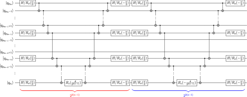
Figure 1: Standard quantum circuit performing a fermionic $n$-tuple particle–hole excitation, $\exp(\theta\kappa_{p_{1}\ldots p_{n}}^{p_{n+1}\ldots p_{2n}})$. The vertical dotted lines denote CNOT “staircases.”

In the majority of quantum computing applications to chemistry, the reference state $\ket*{\Phi}$ appearing in Eq. (3) is a single Slater determinant, typically the Hartree–Fock (HF) determinant, and $U(\mathbf{t})$ is a factorized UCC unitary,

$$U^{(\text{dUCC})}(\mathbf{t})=\prod_{\mu}e^{t_{\mu}\kappa_{\mu}},$$ (7)

which we refer to as disentangled UCC (dUCC) [52]. The $\kappa_{\mu}$ symbols denote anti-Hermitian many-body excitation operators, defined as $\kappa_{\mu}\equiv\kappa_{p_{1}\ldots p_{n}}^{p_{n+1}\ldots p_{2n}}=a^{p_{n+1}}\cdots a^{p_{2n}}a_{p_{n}}\cdots a_{p_{1}}-a^{p_{1}}\cdots a^{p_{n}}a_{p_{2n}}\cdots a_{p_{n+1}}$. Here, the first $n$ indices, namely, $p_{1}<\cdots<p_{n}$, designate spinorbitals occupied in the reference Slater determinant $\ket*{\Phi}$ while the $p_{n+1}<\cdots<p_{2n}$ indices denote unoccupied ones. Note that the presence of de-excitation operators in the UCC wavefunction ansatz implies that the $\kappa_{\mu}$ operators do not necessarily commute among themselves and, consequently, the ordering of the exponentials in $U^{(\text{dUCC})}(\mathbf{t})$ is important.

II.2 Standard Fermionic and Qubit Quantum Circuits

The first step in realizing a quantum chemistry calculation on a quantum computer is to employ a fermionic encoding, enabling one to represent a fermionic problem in the qubit basis. In the Jordan–Wigner (JW) transformation [53], which we employ throughout this study, the fermionic creation ($a^{p}$) and annihilation ($a_{p}$) operators associated with spinorbital $p$ are transformed as

$$a^{p}\xrightarrow{\text{JW}}Q^{p}\prod_{i=0}^{p-1}Z_{i}$$ (8)

and

$$a_{p}\xrightarrow{\text{JW}}Q_{p}\prod_{i=0}^{p-1}Z_{i},$$ (9)

where $Q^{p}\equiv Q_{p}^{\dagger}=\tfrac{1}{2}(X_{p}-iY_{p})$ and $Q_{p}=\tfrac{1}{2}(X_{p}+iY_{p})$ are the corresponding qubit creation and annihilation operators, respectively, and $X_{p}$, $Y_{p}$, and $Z_{p}$ denote Pauli gates acting on the $p^{\text{th}}$ qubit. Under the JW mapping, spinorbital occupation numbers are stored locally in the quantum device while the fermionic sign is encoded non-locally.

Using Eqs. (8) and (9), one can “translate” any fermionic operator from the language of second quantization to linear combinations of Pauli strings acting on qubits. For the purposes of this study, we focus on an element of the dUCC ansatz, Eq. (7), that performs an arbitrary fermionic $n$-tuple particle–hole excitation, $\exp(\theta\kappa_{p_{1}\ldots p_{n}}^{p_{n+1}\ldots p_{2n}})$. It is straightforward to show that

$$\begin{split}e^{\theta\kappa_{p_{1}\ldots p_{n}}^{p_{n+1}\ldots p_{2n}}}&\xrightarrow{\text{JW}}e^{i\frac{\theta}{2^{2n-1}}\left(\sum_{l=1}^{2^{2(n-1)}}P_{l}-\sum_{m=1}^{2^{2(n-1)}}P_{m}\right)}\\ &\xrightarrow{\phantom{\text{JW}}}\prod_{l=1}^{2^{2(n-1)}}e^{i\frac{\theta}{2^{2n-1}}P_{l}}\prod_{m=1}^{2^{2(n-1)}}e^{-i\frac{\theta}{2^{2n-1}}P_{m}},\end{split}$$ (10)

where the $P_{i}$’s denote Pauli strings. In the last step, we utilized the fact that Pauli strings originating from the same second-quantized operator commute [54]. As depicted in Fig. 1, the standard quantum circuit implementing the product of unitaries appearing in Eq. (10) involves a series of single-qubit gates and two-qubit CNOTs. The mathematical expressions for the single- and two-qubit gate counts are provided in Table 1. As shown in Table 1, the number of CNOT gates scales exponentially with the excitation rank $n$, as $\alpha 2^{2n}$, and, to make matters worse, the prefactor $\alpha$ depends on the indices of the spinorbitals involved in the excitation process (a manifestation of the non-local nature of fermionic sign in the JW encoding).

Table 1: Comparison of the numbers of single-qubit gates and CNOTs involved in the various quantum circuits implementing anti-Hermitian $n$-tuple fermionic and qubit particle–hole excitations, $\kappa_{p_{1}\ldots p_{n}}^{p_{n+1}\ldots p_{2n}}$, examined in this work.

Quantum Circuit	Analytic Count: $\kappa_{p_{1}\ldots p_{n}}^{p_{n+1}\ldots p_{2n}}$		Example: $\kappa_{2\;1\;\>\;5}^{8\;9\;11}$
	SQG	CNOT	SQG	CNOT
Standard Fermionic	$\displaystyle(4n+1)2^{2n-1}$	$\displaystyle\left(\sum_{i=0}^{2n-1}{(-1)}^{i}p_{2n-i}+n-1\right){2^{2n}}$	416	512
Standard Qubit	$\displaystyle(4n+1)2^{2n-1}$	$\displaystyle(2n-1)2^{2n}$	416	320
FEB	$\displaystyle 2^{2n-1}$	$\displaystyle 2^{2n-1}+4n-2+2\left(\sum_{p_{2i}-p_{2i-1}>2}(p_{2i}-p_{2i-1}-2)+\sum_{p_{2i}-p_{2i-1}>1}1-\left[\sum_{p_{2i}-p_{2i-1}>1}1>0\right]\right)$	32	46
QEB	$\displaystyle 2^{2n-1}$	$\displaystyle 2^{2n-1}+4n-2$	32	42

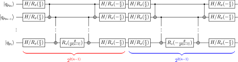
Figure 2: Standard quantum circuit performing a qubit $n$-tuple particle–hole excitation, $\exp(\theta Q_{p_{1}\ldots p_{n}}^{p_{n+1}\ldots p_{2n}})$. The vertical dotted lines denote CNOT “staircases.”

One way to reduce the number of CNOTs is by replacing fermionic excitations $\kappa_{p_{1}\ldots p_{n}}^{p_{n+1}\ldots p_{2n}}$ by their qubit counterparts $Q_{p_{1}\ldots p_{n}}^{p_{n+1}\ldots p_{2n}}\equiv Q^{p_{n+1}}\cdots Q^{p_{2n}}Q_{p_{n}}\cdots Q_{p_{1}}-Q^{p_{1}}\cdots Q^{p_{n}}Q_{p_{2n}}\cdots Q_{p_{n+1}}$, which practically translates to removing the strings of $Z$ gates encoding the fermionic sign in Eqs. (8) and (9). The standard quantum circuit performing an arbitrary qubit $n$-tuple particle–hole excitation is shown in Fig. 2 and the corresponding counts of single-qubit gates and CNOTs are given in Table 1. A quick inspection of Fig. 2 immediately reveals the local nature of qubit excitations since all quantum gates act exclusively on the qubits involved in the excitation process. Although the CNOT gate count is still characterized by the same exponential scaling as in the fermionic case, the replacement of fermionic excitations by their qubit counterparts results in quantum circuits with substantially reduced CNOT counts. For example, the standard quantum circuit performing the qubit triple excitation $Q_{2\;1\;\>\;5}^{8\;9\;11}$ contains about 38% less CNOTs than its fermionic cousin. This is a consequence of the fact that the number of CNOT gates depends only on the excitation rank, e.g., single, double, and triple qubit excitations will give rise to quantum circuits containing 4, 48, and 320 CNOT gates, respectively, independently of the indices involved in the excitation processes.

At this point, it is worth mentioning that the reduction in the CNOT count associated with qubit excitations might come at the cost of possibly sacrificing the proper sign structure of the resulting state. This can be illustrated, for example, by comparing the actions of the fermionic and qubit creation operators, i.e.,

$$a^{p}\ket*{\ldots n_{p}\ldots}=(1-n_{p})(-1)^{\sum_{r=0}^{p-1}n_{r}}\ket*{\ldots 1_{p}\ldots},$$ (11)

$$Q^{p}\ket*{\ldots q_{p}\ldots}=(1-q_{p})\ket*{\ldots 1_{p}\ldots}.$$ (12)

Thus, despite the fact that a wavefunction generated by a qubit approach will have the proper fermionic anti-symmetry, which is inherent to the employed many-electron basis of Slater determinants [45], obtaining the sign structure, up to a phase, of the desired state might not be trivial. This implies that qubit schemes might be potentially characterized by a slower convergence to the FCI solution compared to their fermionic counterparts.

II.3 CNOT-Efficient Single and Double Excitations

The standard quantum circuits performing qubit excitations are not the most economical in terms of CNOT gates. In designing CNOT-efficient quantum circuits for qubit single and double excitations, Yordanov et al. chose a different route [41]. Instead of expressing the qubit creation and annihilation operators in terms of Pauli gates, they examined the action of the entire unitaries performing qubit single and double excitations, namely, $\exp(\theta Q^{p_{2}}_{p_{1}})$ and $\exp(\theta Q^{p_{3}p_{4}}_{p_{1}p_{2}})$, respectively, on an arbitrary multi-qubit basis state. Based on the observation that these unitaries continuously exchange the states $\ket*{1_{p_{1}}0_{p_{2}}}$ and $\ket*{0_{p_{1}}1_{p_{2}}}$ in the case of singles and $\ket*{1_{p_{1}}1_{p_{2}}0_{p_{3}}0_{p_{4}}}$ and $\ket*{0_{p_{1}}0_{p_{2}}1_{p_{3}}1_{p_{4}}}$ for doubles while leaving any other basis state unchanged, Yordanov et al. showed that such controlled exchanges can be performed with the QEB quantum circuits depicted in Fig. 3. After decomposing the multi-qubit-controlled $R_{y}(2\theta)$ gate in terms of CNOTs and single-qubit $R_{y}$ rotations [55, 56, 41], the final quantum circuits contain 4 and 14 CNOTs for qubit single and double excitations, respectively. By taking advantage of circuit identities, the CNOT counts can be decreased to 2 (singles) and 13 (doubles). Thus, the replacement of the standard quantum circuits performing qubit single and double excitations by their QEB counterparts results in a drastic reduction in the number of CNOTs, namely, 50% for singles and about 73% in the case of doubles.

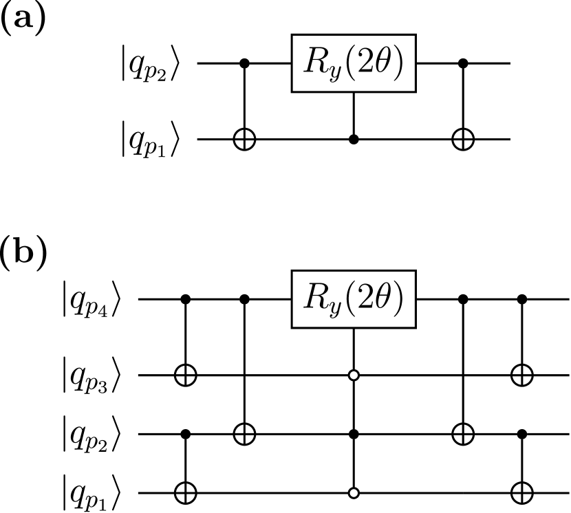
Figure 3: QEB quantum circuits performing (a) single and (b) double particle–hole excitations, $\exp(\theta Q_{p_{1}}^{p_{2}})$ and $\exp(\theta Q_{p_{1}p_{2}}^{p_{3}p_{4}})$, respectively. The open circles denote anti-control qubits.

Yordanov et al. also adapted their QEB quantum circuits for singles and doubles to fermionic excitations by restoring the fermionic sign information. This was accomplished by “sandwiching” the quantum circuits of Fig. 3 between two CNOT “staircases” and two controlled Z (CZ) gates [41]. The resulting CNOT-efficient FEB quantum circuits required only two CNOT “staircases” instead of 4 in the case of singles and 16 for doubles.

II.4 CNOT-Efficient Excitations of Arbitrary Many-Body Rank

Although Yordanov states that this novel approach to constructing CNOT-efficient quantum circuits can be extended to higher-order excitations [57], to the best of our knowledge the pertinent analysis has not been carried out and the corresponding optimal circuits have not been implemented. To generalize the CNOT-efficient quantum circuits shown in Fig. 3 to an arbitrary excitation rank, we follow a procedure similar to the one of Yordanov et al. [41]. We begin by examining the action of a unitary performing a qubit $n$-tuple excitation on a generic multi-qubit basis state,

$$e^{\theta Q^{p_{n+1}\ldots p_{2n}}_{p_{1}\ldots p_{n}}}\ket*{q_{p_{1}}\ldots q_{p_{n}}q_{p_{n+1}}\ldots q_{p_{2n}}}.$$ (13)

In principle, depending on the state of the qubits involved in the excitation process, one would need to examine $2^{2n}$ distinct cases. Nevertheless, by Taylor expanding the exponential, it is straightforward to show that the unitary will leave the $\ket*{q_{p_{1}}\ldots q_{p_{n}}q_{p_{n+1}}\ldots q_{p_{2n}}}$ basis state unchanged unless $q_{p_{1}}=\cdots=q_{p_{n}}\neq q_{p_{n+1}}=\cdots=q_{p_{2n}}$, in which case

$$\begin{split}e^{\theta Q^{p_{n+1}\ldots p_{2n}}_{p_{1}\ldots p_{n}}}\ket*{1_{p_{1}}\ldots 1_{p_{n}}0_{p_{n+1}}\ldots 0_{p_{2n}}}\\ =\quad\cos(\theta)\ket*{1_{p_{1}}\ldots 1_{p_{n}}0_{p_{n+1}}\ldots 0_{p_{2n}}}\\ +\sin(\theta)\ket*{0_{p_{1}}\ldots 0_{p_{n}}1_{p_{n+1}}\ldots 1_{p_{2n}}}\end{split}$$ (14)

and

$$\begin{split}e^{\theta Q^{p_{n+1}\ldots p_{2n}}_{p_{1}\ldots p_{n}}}\ket*{0_{p_{1}}\ldots 0_{p_{n}}1_{p_{n+1}}\ldots 1_{p_{2n}}}\\ =\quad-\sin(\theta)\ket*{1_{p_{1}}\ldots 1_{p_{n}}0_{p_{n+1}}\ldots 0_{p_{2n}}}\\ +\cos(\theta)\ket*{0_{p_{1}}\ldots 0_{p_{n}}1_{p_{n+1}}\ldots 1_{p_{2n}}}\end{split}.$$ (15)

Thus, similarly to single and double qubit excitations, the $\exp(\theta Q^{p_{n+1}\ldots p_{2n}}_{p_{1}\ldots p_{n}})$ unitary continuously exchanges the $\ket*{1_{p_{1}}\ldots 1_{p_{n}}0_{p_{n+1}}\ldots 0_{p_{2n}}}$ and $\ket*{0_{p_{1}}\ldots 0_{p_{n}}1_{p_{n+1}}\ldots 1_{p_{2n}}}$ basis states while acting as the identity otherwise. The resemblance of Eqs. (14) and (15) to the action of the single-qubit $R_{y}(2\theta)$ gate on the $\ket*{0}$ and $\ket*{1}$ states, respectively, allows us to construct the CNOT-efficient QEB quantum circuit shown in Fig. 4. The CNOT gates to the left of the multi-qubit-controlled $R_{y}(2\theta)$ gate ensure that the circuit will only act non-trivially on the two aforementioned basis states. This can be seen as follows. The cascade of $n-1$ CNOT gates between $q_{p_{n}}$ and the remaining $q_{p_{m}},m=1,\ldots,n-1$, qubits checks whether each of the $q_{p_{m}}$ qubits is in the same quantum state as $q_{p_{n}}$; the action of the CNOT gate will result in qubit $q_{p_{m}}$ being in the $\ket*{0}$ state if $q_{p_{n}}$ and $q_{p_{m}}$ are in the same state, otherwise $q_{p_{m}}=\ket*{1}$. The cascade of $n-1$ CNOTs between $q_{p_{2n}}$ and the remaining $q_{p_{m}},m=n+1,\ldots,2n-1$, qubits acts in a similar manner. The single CNOT gate entangling qubits $q_{p_{2n}}$ and $q_{p_{n}}$ checks whether these two qubits are in the same quantum state. Consequently, the multi-qubit-controlled $R_{y}(2\theta)$ gate will only be applied if the following three conditions are satisfied: $q_{p_{1}}=\cdots=q_{p_{n}}$, $q_{p_{n+1}}=\cdots=q_{p_{2n}}$, and $q_{p_{n}}\neq q_{2n}$. This analysis justifies the choice of control vs anti-control qubits in the multi-qubit-controlled $R_{y}(2\theta)$ gate. If the multi-qubit-controlled $R_{y}(2\theta)$ gate is not applied, then the CNOT gates to its right will pairwise cancel with the CNOT gates to its left, leaving the system in the same quantum state. Otherwise, the CNOT gates to the right of the multi-qubit-controlled $R_{y}(2\theta)$ gate complete the desired transformation.

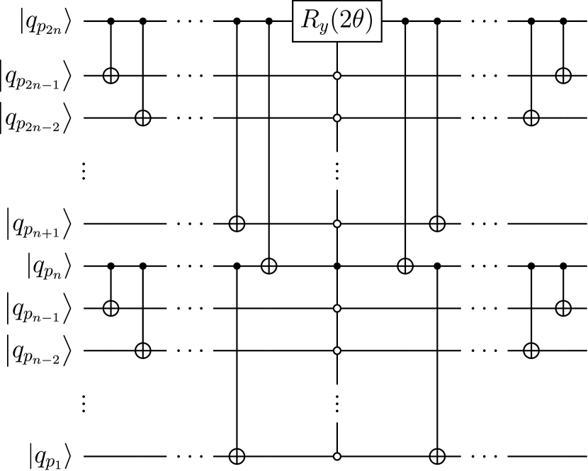
Figure 4: QEB quantum circuit performing a qubit $n$-tuple particle–hole excitation, $\exp(\theta Q_{p_{1}\ldots p_{n}}^{p_{n+1}\ldots p_{2n}})$.

Figure 5: FEB quantum circuit performing a fermionic $n$-tuple particle–hole excitation, $\exp(\theta\kappa_{p_{1}\ldots p_{n}}^{p_{n+1}\ldots p_{2n}})$. The parameter $f$ controlling the sign of the rotation angle depends on the excitation rank $n$ as follows: $f=0$ for $n=1,4,5,8,9,\ldots$ and $f=1$ for $n=2,3,6,7,\ldots$.

As demonstrated in Sec. SI of the Supplemental Material, the decomposition of the multi-qubit-controlled $R_{y}(2\theta)$ gate introduces an exponential number of single-qubit gates and CNOTs, thus dominating the pertinent total counts reported in Table 1. Nevertheless, the QEB quantum circuit offers a dramatic reduction in both the numbers of single-qubit gates and CNOTs when compared to those characterizing its traditional counterpart. Furthermore, the reductions become more impressive as the excitation rank becomes larger. For example, the QEB implementations of qubit triple, quadruple, pentuple, and hextuple excitations require about 92%, 94%, 95%, and 96% less single-qubit gates and 87%, 92%, 94%, and 95% fewer CNOTs, respectively, when compared to the corresponding standard qubit quantum circuits. At this point, it is worth mentioning that, similarly to the QEB singles and doubles case, one can utilize circuit identities to reduce the number of CNOTs by 1 when decomposing the multi-qubit-controlled $R_{y}(2\theta)$ gate. However, as outlined in Sec. SII in the Supplemental Material, these circuit identities introduce a number of single-qubit gates that scales linearly with the excitation rank, essentially outweighing the benefits of reducing the operational noise by removing a single CNOT, especially so for higher-rank excitations. Consequently, our implementation produces QEB quantum circuits with the single-qubit and CNOT gate counts shown in Table 1, which we believe offer the best balance between CNOTs and overall gate errors.

The FEB quantum circuit performing a CNOT-efficient fermionic $n$-tuple excitation is shown in Fig. 5. In addition to the two extra CNOT “staircases” and CZ gates considered by Yordanov et al., a close inspection of Fig. 5 reveals a further modification with respect to the QEB quantum circuit of Fig. 4. Due to the fact that fermions and qubits do not obey the same algebras [58], we found that the angle of the multi-qubit-controlled $R_{y}$ gate contains a sign factor that depends on the excitation rank $n$ in a rather non-intuitive way, namely, $+1$ for $n=1,4,5,8,9,\ldots$ and $-1$ in the case of $n=2,3,6,7,\ldots$.

As shown in Table 1, the use of an FEB quantum circuit instead of its standard counterpart results in a dramatic decrease in the number of CNOT gates. For example, the FEB quantum circuit performing the $\kappa_{2\;1\;\>\;5}^{8\;9\;11}$ fermionic triple excitation contains 91% less CNOTs than its standard analog. A quick comparison of Figs. 1 and 5 reveals that the impressive decrease in the number of CNOTs can be partly attributed to the fact that the standard circuit performing fermionic excitations contains a number of CNOT “staircases” that scales exponentially with the excitation rank $n$ while its FEB analog requires only two “staircases”, independently of $n$. An FEB quantum circuit typically contains a number of CNOT gates that is greater than that of its QEB counterpart. Nevertheless, the disparity between the FEB and QEB CNOT counts depends on two factors, namely, the excitation rank $n$ and the indices involved in the excitation process. In general, for lower-rank excitations, such as singles and doubles, the two extra CNOT “staircases” are expected to be the primary source of CNOTs in an FEB circuit, maximizing the difference between the FEB and QEB CNOT counts. As the excitation rank increases, the FEB CNOT count is dominated by the multi-qubit-controlled $R_{y}$ gate, bridging the gap with respect to its QEB analog. Furthermore, in the case of consecutive excitation indices, the FEB and QEB quantum circuits will contain the same number of CNOT gates.

III Results and Discussion

The discussion of our numerical results is divided into three parts. We begin in Sec. III.1 by examining the savings in terms of CNOT gates offered by the FEB- and QEB-SPQE approaches introduced in this work compared to their standard fermionic SPQE and qubit qSPQE analogs. Subsequently, in Sec. III.2, we compare the performance of the FEB-SPQE scheme with its QEB counterpart in terms of four different metrics, namely, errors with respect to FCI, number of parameters in the ansatz, CNOT counts, and number of residual element evaluations. We conclude the discussion of our results in Sec. III.3 with a comparison of the most CNOT-efficient SPQE and ADAPT-VQE variants considered in this study.

All SPQE computations discussed in this section employed a selection threshold of $\Omega=${10}^{-2}\text{\,}\textit{E}_{\mathrm{h}}$$ (see Appendix A for the algorithmic details of the recently proposed SPQE scheme). The ADAPT-VQE simulations reported here used a selection criterion of ${10}^{-3}\text{\,}\textit{E}_{\mathrm{h}}$. Additional values of the SPQE and ADAPT-VQE selection thresholds have been considered in the Supplemental Material. The remaining computational details can be found in Appendix B.

III.1 Standard vs CNOT-Efficient SPQE

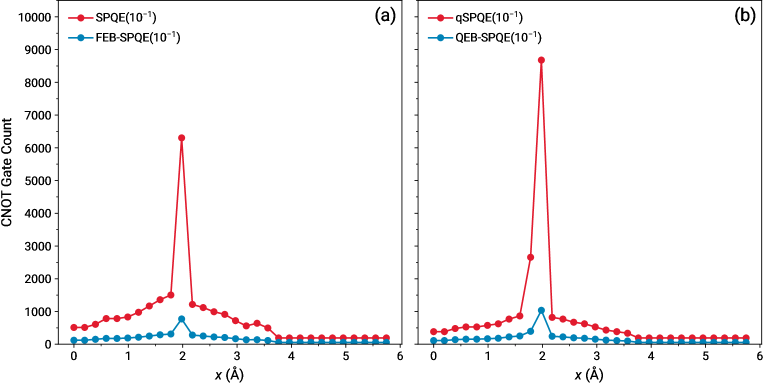
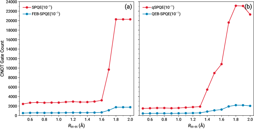
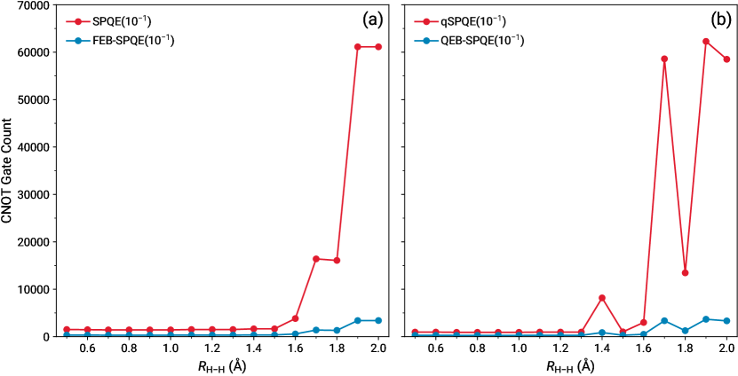
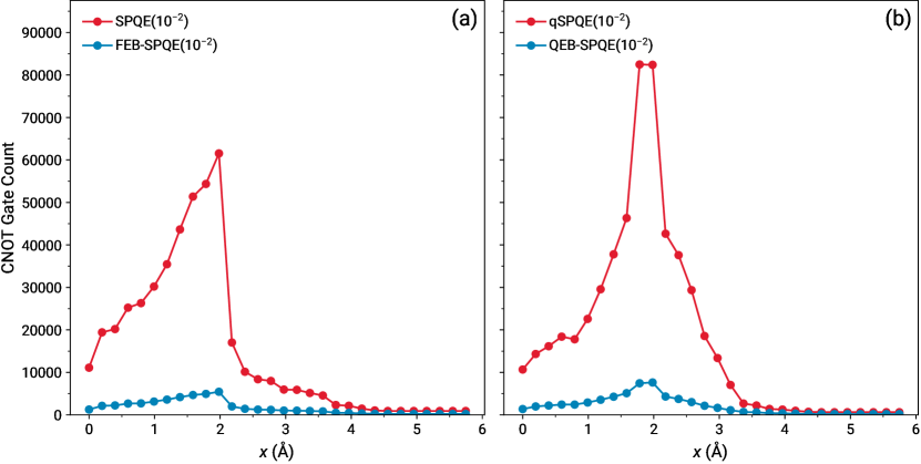
Figure S10: Total CNOT gate counts characterizing the (a) fermionic SPQE and FEB-SPQE and (b) qubit qSPQE and QEB-SPQE ansatz unitaries for the insertion of Be into $\text{H}_{2}$. All computations employ a selection threshold of $\Omega=${10}^{-1}\text{\,}\textit{E}_{\mathrm{h}}$$.

Figure S11: Total CNOT gate counts characterizing the (a) fermionic SPQE and FEB-SPQE and (b) qubit qSPQE and QEB-SPQE ansatz unitaries for the symmetric dissociation of the linear $\text{H}_{6}$/STO-6G system. All computations employ a selection threshold of $\Omega=${10}^{-1}\text{\,}\textit{E}_{\mathrm{h}}$$.

Figure S12: Total CNOT gate counts characterizing the (a) fermionic SPQE and FEB-SPQE and (b) qubit qSPQE and QEB-SPQE ansatz unitaries for the symmetric dissociation of the $\text{H}_{6}$/STO-6G ring. All computations employ a selection threshold of $\Omega=${10}^{-1}\text{\,}\textit{E}_{\mathrm{h}}$$.

Figure S13: Total CNOT gate counts characterizing the (a) fermionic SPQE and FEB-SPQE and (b) qubit qSPQE and QEB-SPQE ansatz unitaries for the insertion of Be into $\text{H}_{2}$. All computations employ a selection threshold of $\Omega=${10}^{-2}\text{\,}\textit{E}_{\mathrm{h}}$$.

The numbers of CNOT gates characterizing the various standard and CNOT-efficient SPQE computations of the symmetric dissociations of the linear $\text{BeH}_{2}$/STO-6G and $\text{H}_{6}$/STO-6G systems are shown in Fig. 6. A quick inspection of Fig. 6 reveals that the reduction in the CNOT count offered by the FEB- and QEB-SPQE approaches compared to their standard SPQE and qSPQE counterparts is significant. Indeed, the replacement of the conventional quantum circuits representing $n$-tuple fermionic (Fig. 1) and qubit (Fig. 2) excitations with their FEB (Fig. 5) and QEB (Fig. 4) variants results in about 6–12 times less CNOTs in the case of $\text{BeH}_{2}$ and 8–15 times for $\text{H}_{6}$. This is true not only for the equilibrium region of the potential energy curves (PECs), characterized by weaker many-electron correlation effects, but also for the stretched geometries, where non-dynamical correlations become prevalent. What is even more intriguing is the fact that as the strength of the correlation effects increases, the savings in the number of CNOTs become more substantial. This can be understood in the following manner. As one departs from the weakly correlated regime, the $n$-body excitation operators with $n>2$ become important enough to satisfy the SPQE selection criterion. At the same time, the efficacy of the FEB and QEB quantum circuits to reduce the number of CNOTs is an increasing function of the excitation rank $n$, giving rise to the observed behavior (see Sec. II.4). Although here we focused on the symmetric dissociation of the linear $\text{BeH}_{2}$ and $\text{H}_{6}$ systems, similar observations can be made in the case of the insertion of Be into $\text{H}_{2}$ and the symmetric dissociation of the $\text{H}_{6}$ ring (see Figs. S13 and S14 in the Supplemental Material).

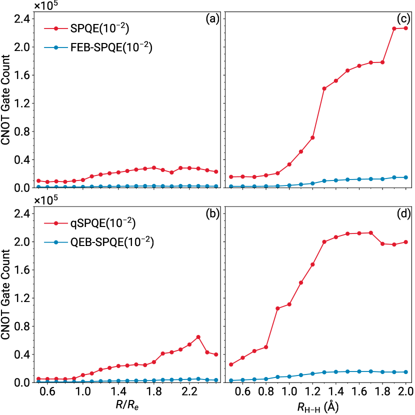
Figure 6: Total CNOT gate counts characterizing the fermionic SPQE and FEB-SPQE [(a) and (c)] and qubit qSPQE and QEB-SPQE [(b) and (d)] ansatz unitaries for the symmetric dissociations of the linear $\text{BeH}_{2}$ (left column) and $\text{H}_{6}$ (right column) systems as described by the STO-6G basis.

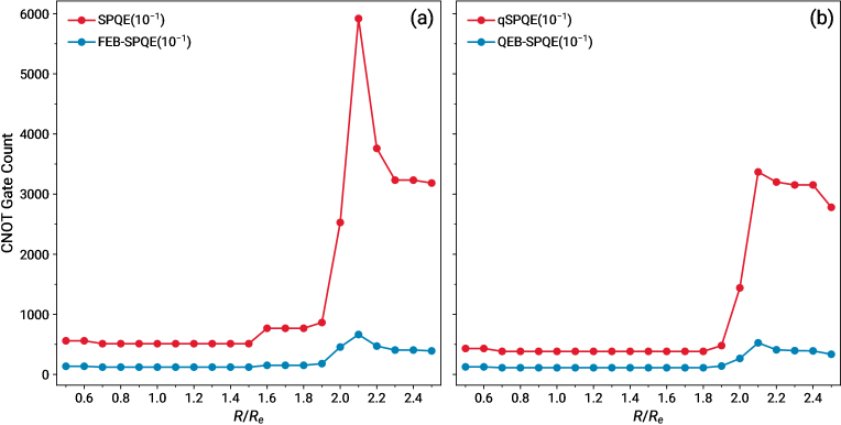
Figure S9: Total CNOT gate counts characterizing the (a) fermionic SPQE and FEB-SPQE and (b) qubit qSPQE and QEB-SPQE ansatz unitaries for the symmetric dissociation of the linear $\text{BeH}_{2}$/STO-6G system. All computations employ a selection threshold of $\Omega=${10}^{-1}\text{\,}\textit{E}_{\mathrm{h}}$$.

The above discussion demonstrates that both the FEB- and QEB-SPQE schemes give rise to quantum circuits containing a remarkably smaller number of CNOT gates when compared to those obtained with their conventional counterparts. More importantly, the savings in terms of CNOTs are anticipated to be even more pronounced in situations involving stronger many-electron correlation effects. Furthermore, as illustrated in the Supplemental Material, similarly impressive reductions in the CNOT counts are also observed when one employs the less tight importance criterion of $\Omega=${10}^{-1}\text{\,}\textit{E}_{\mathrm{h}}$$ (see Figs. S9–S12). Next, we turn our attention to the comparison of the FEB and QEB flavors of SPQE among themselves.

III.2 FEB-SPQE vs QEB-SPQE

The purpose of this section is to determine which of the two CNOT-efficient variants of SPQE offers the best balance between accuracy and required computational resources. To gauge the accuracy of the fermionic FEB-SPQE approach and its qubit QEB analog, we compare the resulting energetics with those obtained from FCI. In estimating the overall computational costs of the FEB- and QEB-SPQE schemes, we consider three metrics, namely, the number of operators involved in the converged unitary, the number of CNOT gates contained in the quantum circuit representing the unitary, and the total number of residual element evaluations characterizing the entire SPQE simulation.

In Fig. 7, we examine how the FEB- and QEB-SPQE schemes perform when applied to the symmetric dissociations of the linear $\text{BeH}_{2}$ and $\text{H}_{6}$ species, as described by the STO-6G basis set. We begin our comparison with a discussion of the pertinent energetics. As illustrated in panels (a) and (e) of Fig. 7, the energies resulting from the FEB- and QEB-SPQE simulations are not only more or less identical among themselves, but also in excellent agreement with those obtained with FCI. Indeed, both CNOT-efficient flavors of SPQE reproduce the exact, FCI, data to within a fraction of a millihartree, independently of the strength of the many-electron correlation effects. This is even true for the dissociating $\text{H}_{6}$ linear chain, a prototypical system of strong correlations. In this case, although the errors with respect to FCI increase as one approaches the dissociation limit, they typically remain one order of magnitude below of what is known as “chemical accuracy,” namely, $1\text{\,}\mathrm{m}\textit{E}_{\mathrm{h}}$. At a first glance, it might seem surprising that QEB-SPQE, which by construction neglects the proper fermionic signs, is as accurate as its fermionic counterpart, especially so in situations characterized by substantial non-dynamical correlation effects. This behavior is a consequence of the tight cumulative threshold of $\Omega=${10}^{-2}\text{\,}\textit{E}_{\mathrm{h}}$$, which enables both FEB- and QEB-SPQE to practically recover the FCI solution. Nevertheless, additional insights in this aspect can be gained by examining the number of ansatz parameters.

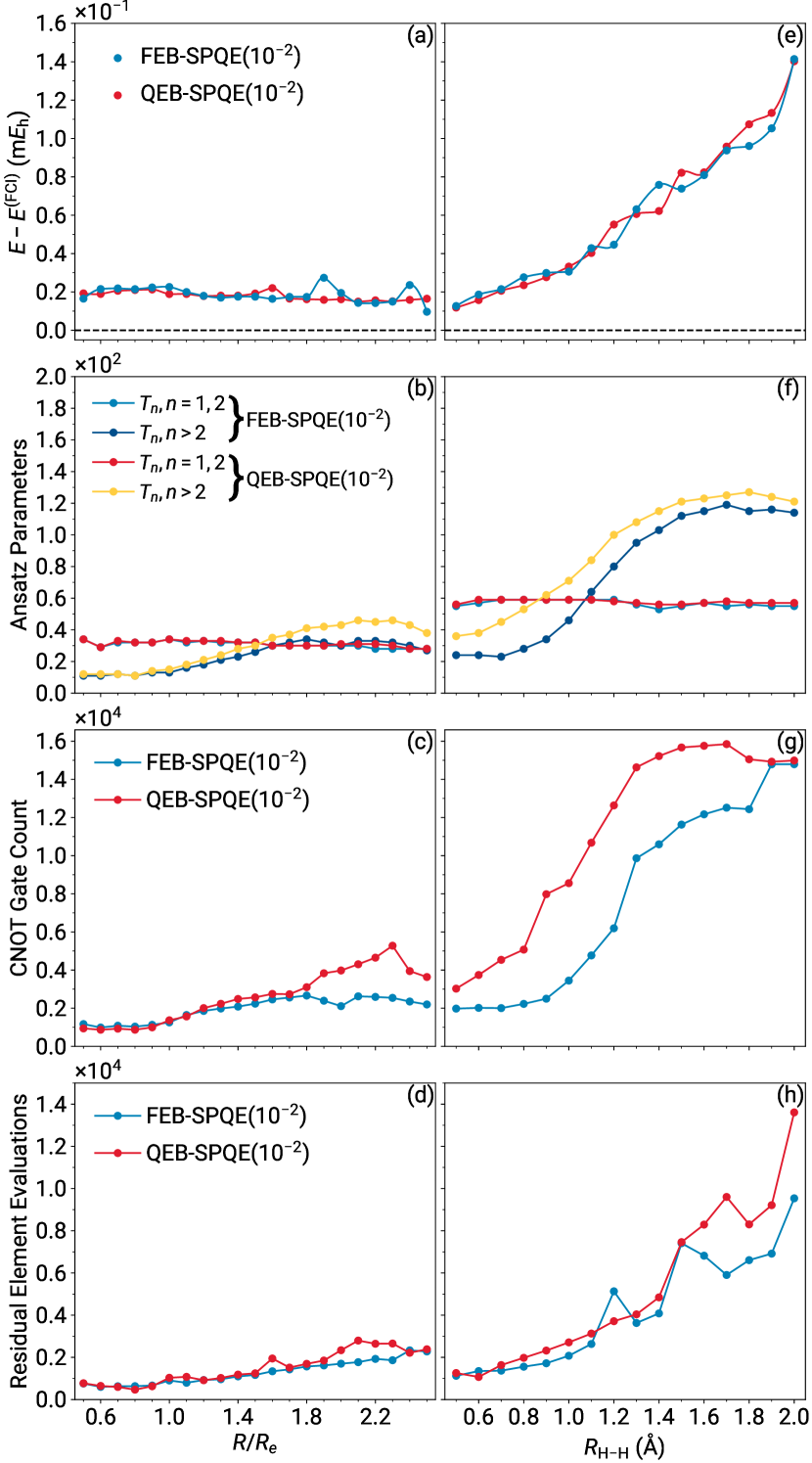
Figure 7: Errors relative to FCI [(a) and (e)], ansatz parameters [(b) and (f)], CNOT gate counts [(c) and (g)], and residual element evaluations [(d) and (h)] characterizing the FEB- and QEB-SPQE simulations of the symmetric dissociations of the linear $\text{BeH}_{2}$ (left column) and $\text{H}_{6}$ (right column) systems as described by the STO-6G basis.

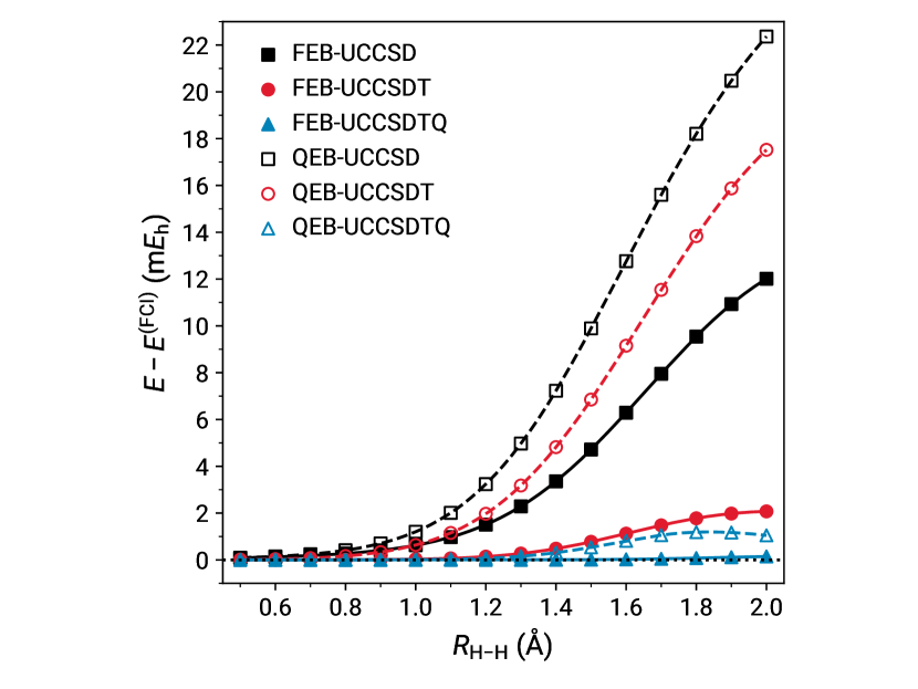
Figure S8: Errors relative to FCI characterizing the FEB-UCCSD, FEB-UCCSDT, FEB-UCCSDTQ, QEB-UCCSD, QEB-UCCSDT, and QEB-UCCSDTQ simulations of the symmetric dissociation of the $\text{H}_{6}$ linear chain as described by the STO-6G basis.

A quick inspection of panels (b) and (f) of Fig. 7 reveals that the QEB-SPQE method produces less compact ansätze when compared to the FEB variant, in particular when many-electron correlation effects become significant. To make matters worse, although the FEB- and QEB-SPQE unitaries contain roughly the same number of single and double excitation operators, QEB-SPQE requires a larger number of $n$-tuple excitations with $n>2$ to reach convergence. The explanation of this behavior lies in the fact that qubit excitation operators do not account for proper fermionic signs. Therefore, as far as the number of ansatz parameters is concerned, it is anticipated that qubit approaches will be characterized by a less rapid convergence to the FCI solution when compared to their fermionic analogs. As an extreme example of this slower convergence, in Fig. S8 we present the errors relative to FCI characterizing the energies obtained with the fermionic FEB-UCCSD, FEB-UCCSDT, and FEB-UCCSDTQ schemes and their qubit counterparts for the symmetric dissociation of the $\text{H}_{6}$/STO-6G linear chain. In this particular case, the FEB-UCCSD energetics are, in general, more accurate than those obtained with the nominally higher-level QEB-UCCSDT scheme. Despite the dramatic improvement arising from the incorporation of quadruples, the QEB-UCCSDTQ approach gives rise to a PEC that is only slightly better than that obtained with FEB-UCCSDT. At the same time, the fermionic FEB-UCCSDTQ potential can hardly be distinguished from its FCI counterpart. These observations highlight the fact that higher–than–two-body excitation operators are needed to restore the proper fermionic sign structure in a many-fermion wavefunction obtained with a qubit ansatz.

Although FEB-SPQE leads to more compact ansätze compared to its QEB variant, it is not immediately obvious that it will be more CNOT-efficient. To be precise, the CNOT count depends not only on the number of operators incorporated in the ansatz unitary, but also on their identity, i.e., the many-body ranks of the operators and the indices involved in the excitation processes. As discussed in Sec. II.4, the number of CNOT gates contained in a quantum circuit implementing an $n$-tuple fermionic/qubit excitation scales exponentially with $n$. Since QEB-SPQE gives rise to unitaries that typically include a larger number of higher–than–two-body excitations than its FEB analog, FEB-SPQE is anticipated to be, in general, more economical in terms of CNOTs. As illustrated in panels (c) and (g) of Fig. 7, this is indeed the case, especially in situations involving substantial non-dynamic correlation effects. For example, for the dissociating $\text{H}_{6}$ linear chain, a prototypical strongly correlated system, the FEB-SPQE approach requires on average 36% less CNOTs than its QEB counterpart. However, the case of the symmetric dissociation of the linear $\text{BeH}_{2}$ species is not as straightforward. If we focus on the geometries where both Be–H bonds are stretched to about twice their equilibrium distance or more, a similar picture to $\text{H}_{6}$ emerges, with the FEB-SPQE CNOT counts being on average 43% smaller than the QEB ones. The situation reverses in favor of QEB-SPQE when one examines the equilibrium region of the $\text{BeH}_{2}$ potential, which is characterized by weaker many-electron correlation effects. In this case, despite the fact that the FEB-SPQE ansätze are marginally more compact than their QEB counterparts, the QEB-SPQE quantum circuits contain a slightly smaller number of CNOT gates compared to those resulting from FEB-SPQE. This behavior can be understood by examining the operators included in the FEB- and QEB-SPQE unitaries. For these compressed geometries, QEB-SPQE typically incorporates one or two additional triple excitations with respect to their FEB analogs. Nevertheless, the number of CNOT gates introduced by a couple of qubit triple excitation operators is not enough to outweigh the number of CNOTs associated with the CNOT “staircases” in the fermionic case. This further emphasizes the point that, when comparing FEB and QEB approaches, a more compact ansatz may not necessarily translate into a more CNOT-efficient quantum circuit.

As a final test of the performance of the FEB- and QEB-SPQE approaches, we compare the total number of residual element evaluations characterizing the various simulations. As demonstrated in panels (d) and (h) of Fig. 7, FEB-SPQE requires, in general, slightly fewer residual element evaluations than its QEB counterpart. This can be rationalized based on the fact that the QEB-SPQE ansätze typically contain a larger number of parameters.

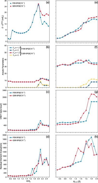
Figure S15: Errors relative to FCI [(a) and (e)], ansatz parameters [(b) and (f)], CNOT gate counts [(c) and (g)], and residual element evaluations [(d) and (h)] characterizing the FEB- and QEB-SPQE simulations of the symmetric dissociations of the linear $\text{BeH}_{2}$ (left column) and $\text{H}_{6}$ (right column) systems as described by the STO-6G basis.

At this point, it is worth mentioning that the above observations regarding the efficiency of the FEB- and QEB-SPQE schemes may depend on the value of the cumulative importance criterion $\Omega$. For example, as shown in Fig. S15 using the symmetric dissociations of the linear $\text{BeH}_{2}$/STO-6G and $\text{H}_{6}$/STO-6G systems, the more relaxed $\Omega=${10}^{-1}\text{\,}\textit{E}_{\mathrm{h}}$$ threshold results in the distinct advantage of FEB-SPQE over QEB-SPQE being all but lost. In this case, the FEB- and QEB-SPQE ansätze typically contain more or less the same number of parameters. As a result, in general, QEB-SPQE gives rise to quantum circuits with fewer CNOT gates compared to their FEB counterparts, the only exception being the stretched geometries of $\text{H}_{6}$. Finally, although both the FEB- and QEB-SPQE schemes utilize much fewer computational resources compared to their $\Omega=${10}^{-2}\text{\,}\textit{E}_{\mathrm{h}}$$ analogs, they are plagued by substantial errors with respect to the exact energies.

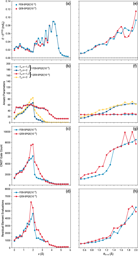
Figure S17: Errors relative to FCI [(a) and (e)], ansatz parameters [(b) and (f)], CNOT gate counts [(c) and (g)], and residual element evaluations [(d) and (h)] characterizing the FEB- and QEB-SPQE simulations of the insertion of Be to $\text{H}_{2}$ (left column) and the symmetric dissociation of the $\text{H}_{6}$ ring (right column) as described by the STO-6G basis.

Based on the above analysis, it is evident that FEB-SPQE with $\Omega=${10}^{-2}\text{\,}\textit{E}_{\mathrm{h}}$$ offers the best overall performance. It not only generates the energies that faithfully reproduce those obtained from FCI, but it also produces compact ansätze leading to decreased CNOT counts. Although here we focused on the symmetric dissociations of the linear $\text{BeH}_{2}$ and $\text{H}_{6}$ systems, more or less similar observations can be made when one examines the insertion of Be into $\text{H}_{2}$ and the symmetric dissociation of the $\text{H}_{6}$ ring (see Fig. S17 in the Supplemental Material).

III.3 FEB-SPQE vs QEB-ADAPT-VQE

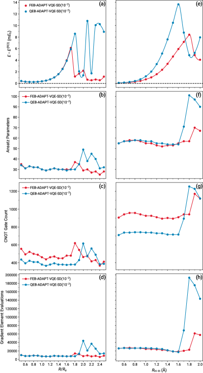
Figure S18: Errors relative to FCI [(a) and (e)], ansatz parameters [(b) and (f)], CNOT gate counts [(c) and (g)], and gradient element evaluations [(d) and (h)] characterizing the FEB- and QEB-ADAPT-VQE-SD simulations of the symmetric dissociations of the linear $\text{BeH}_{2}$ (left column) and $\text{H}_{6}$ (right column) systems as described by the STO-6G basis.

Having established that, among the SPQE flavors examined in this work, FEB-SPQE with $\Omega=${10}^{-2}\text{\,}\textit{E}_{\mathrm{h}}$$ offers the best balance between accuracy and computational cost, we now proceed to compare its performance against that of ADAPT-VQE. In an effort to achieve a fair comparison, we first set out to determine which of the FEB and QEB versions of ADAPT-VQE is the most efficient, i.e., giving rise to quantum circuits with fewer CNOT gates while producing energies within chemical accuracy. A simple inspection of Figs. S18–S25 in the Supplemental Material reveals that, among the tested ADAPT-VQE schemes, only FEB- and QEB-ADAPT-VQE-GSD with a selection threshold of ${10}^{-3}\text{\,}\textit{E}_{\mathrm{h}}$ consistently generate energetics within $1\text{\,}\mathrm{m}\textit{E}_{\mathrm{h}}$ absolute error from FCI. At the same time, QEB-ADAPT-VQE-GSD yields, in general, unitaries with a few hundred CNOT gates less. This is true despite the fact that QEB-ADAPT-VQE-GSD typically gives rise to less compact ansätze than its FEB counterpart. Nevertheless, the CNOT gates associated with the additional single and double qubit excitation operators are not enough to outweigh those arising from the CNOT “staircases” in the fermionic case. Similar observations regarding the efficiencies of FEB- and QEB-ADAPT-VQE were made by Yordanov et al. [42]. Consequently, in what follows, we compare the performance of the FEB-SPQE and QEB-ADAPT-VQE-GSD schemes with selection thresholds of ${10}^{-2}\text{\,}\textit{E}_{\mathrm{h}}$ and ${10}^{-3}\text{\,}\textit{E}_{\mathrm{h}}$, respectively. For the sake of completeness, we also include the corresponding results obtained with the less accurate QEB-ADAPT-VQE-SD approach, the best ADAPT-VQE scheme considered in this study using a pool of particle–hole singles and doubles.

In Fig. 8, we present the results of our numerical simulations for the symmetric dissociations of the linear $\text{BeH}_{2}$/STO-6G and $\text{H}_{6}$/STO-6G systems as obtained with the FEB-SPQE, QEB-ADAPT-VQE-SD, and QEB-ADAPT-VQE-GSD approaches. As was the case with the comparison between the FEB and QEB flavors of SPQE, in order to judge which scheme offers the best balance between accuracy of the computed energies and required computational resources, we rely on four metrics, namely, errors relative to the exact, FCI, energies, compactness of the ansätze, number of CNOT gates contained in the quantum circuits representing the ansatz unitaries, and number of residual [FEB-SPQE] and gradient [QEB-ADAPT-VQE-SD, QEB-ADAPT-VQE-GSD] element evaluations.

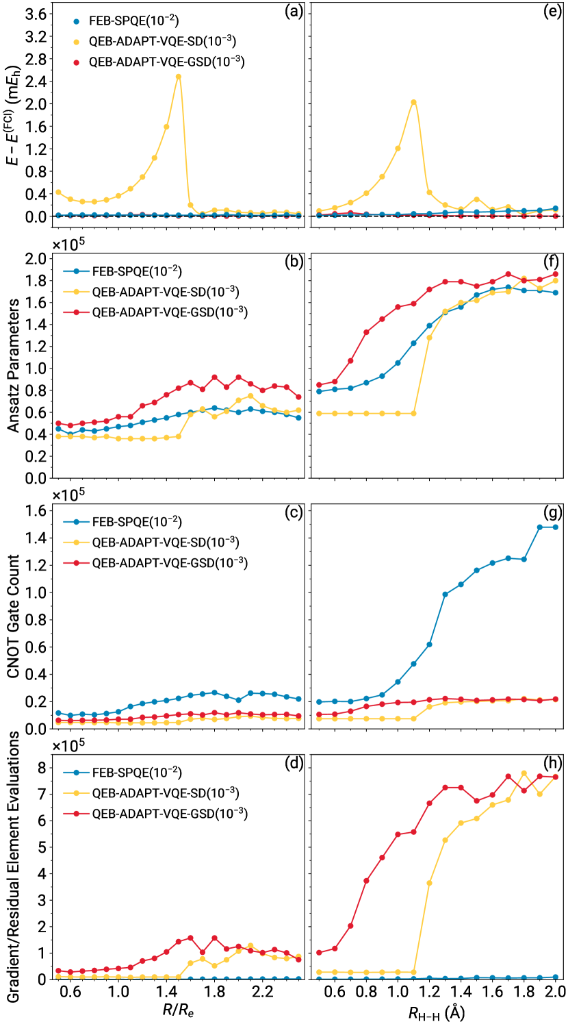
Figure 8: Errors relative to FCI [(a) and (e)], ansatz parameters [(b) and (f)], CNOT gate counts [(c) and (g)], and gradient/residual element evaluations [(d) and (h)] characterizing the FEB-SPQE, QEB-ADAPT-VQE-SD, and QEB-ADAPT-VQE-GSD simulations of the symmetric dissociations of the linear $\text{BeH}_{2}$ (left column) and $\text{H}_{6}$ systems (right column) as described by the STO-6G basis.

We begin our discussion with a comparison of the energetics. A quick inspection of panels (a) and (e) of Fig. 8 immediately reveals that QEB-ADAPT-VQE-SD is the least accurate among the three examined schemes. Indeed, the errors relative to FCI characterizing the QEB-ADAPT-VQE-SD simulations are much larger than those resulting from QEB-ADAPT-VQE-GSD and FEB-SPQE. To make matters worse, QEB-ADAPT-VQE-SD is characterized by maximum errors that exceed $2\text{\,}\mathrm{m}\textit{E}_{\mathrm{h}}$, i.e., more than two times larger than what is known as chemical accuracy, even in the less complicated case of $\text{BeH}_{2}$. Switching to an operator pool of generalized singles and doubles dramatically improves the results. In fact, the QEB-ADAPT-VQE-GSD scheme produces PECs for the symmetric dissociations of the linear $\text{BeH}_{2}$/STO-6G and $\text{H}_{6}$/STO-6G systems that can hardly be distinguished from those resulting from the exact, FCI, calculations. The FEB-SPQE approach is competitive with QEB-ADAPT-VQE-GSD in the weakly correlated regime and in situations involving moderately strong correlations. Indeed, the FEB-SPQE and QEB-ADAPT-VQE-GSD energies are more or less identical, differing by just a few microhartrees, in the case of the double-bond dissociation of the linear $\text{BeH}_{2}$ species and for the equilibrium region of the $\text{H}_{6}$ potential. Although as one approaches the strong correlation limit in the latter case FEB-SPQE becomes somewhat less accurate than QEBADAPT-VQE-GSD, it remains practically one order of magnitude below what is considered chemical accuracy.

We now turn our attention to the numbers of ansatz parameters. As shown in panels (b) and (f) of Fig. 8, the least accurate QEB-ADAPT-VQE-SD scheme produces, in general, the most compact ansätze, typically incorporating fewer excitation operators than FEB-SPQE and QEB-ADAPT-VQE-GSD. At the other end of the spectrum, QEB-ADAPT-VQE-GSD, which faithfully reproduces the exact, FCI, energies, requires the largest number of operators to reach convergence. FEB-SPQE always requires fewer, some times much fewer, ansatz parameters than QEB-ADAPT-VQE-GSD, but typically more than QEB-ADAPT-VQE-SD. Nevertheless, it is worth mentioning that in situations involving significant non-dynamic correlation effects, FEB-SPQE becomes competitive with QEB-ADAPT-VQE-SD, even generating the most compact ansätze for a few nuclear configurations.

Despite the excellent performance of FEB-SPQE in terms of energetics and ansatz parameters, it always generates quantum circuits containing more CNOT gates than both of the examined flavors of ADAPT-VQE. As illustrated in panels (c) and (g) of Fig. 8, the disparity between the FEB-SPQE and QEB-ADAPT-VQE-SD and QEB-ADAPT-VQE-GSD CNOT counts is exacerbated as the strength of non-dynamic correlation effects increases. For example, focusing on the strongly correlated $\text{H}_{6}$ linear chain and the largest H–H separation considered in this work, namely, $R_{\text{H--H}}=$2.0\text{\,}\AA$$, FEB-SPQE requires about seven times more CNOT gates than QEB-ADAPT-VQE-SD or its GSD counterpart. As might have been anticipated, the source behind the disparity in the CNOT counts can be traced to the identities of the excitation operators included in the respective operator pools. In the ADAPT-VQE simulations shown in Fig. 8 we use only (generalized) single and double excitations while in the case of SPQE we employ a full operator pool, including up to $N$-tuple excitation operators, where $N$ is the number of correlated electrons. In light of the fact that the number of CNOT gates introduced by a given $n$-tuple excitation operator scales exponentially with the many-body rank $n$, it is not surprising that FEB-SPQE requires, in general, many more CNOT gates than QEB-ADAPT-VQE-SD or its GSD variant. To put it into perspective, the quantum circuit implementation of the single hextuple excitation in $\text{H}_{6}$/STO-6G, which is incorporated in the FEB-SPQE ansatz already at the $R_{\text{H--H}}=$1.3\text{\,}\AA$$ distance between neighboring H atoms, requires essentially the same number of CNOTs as that needed for the entire QEB-ADAPT-VQE-SD or QEB-ADAPT-VQE-GSD unitaries. Nevertheless, it is worth mentioning that, for the same reason, the savings in terms of CNOTs afforded by the replacement of the standard fermionic and qubit quantum circuits by their FEB and QEB counterparts, respectively, are more impressive in SPQE than ADAPT-VQE. Consequently, by just utilizing the CNOT-efficient FEB and QEB quantum circuits instead of their conventional analogs, we were able to reduce the disparity in the number of CNOT gates between SPQE and ADAPT-VQE from a factor of $\sim 15$ [17] to a factor of $\sim 7$.

As a final gauge of the computational resources needed by SPQE and ADAPT-VQE simulations, we compare the total numbers of residual [FEB-SPQE] and gradient [QEB-ADAPT-VQE-SD, QEB-ADAPT-VQE-GSD] element evaluations. As illustrated in panels (d) and (h) of Fig. 8, QEB-ADAPT-VQE-SD and its GSD counterpart typically require one to two orders of magnitude more gradient element evaluations than the number of residual element measurements in FEB-SPQE. This colossal difference can be largely attributed to the use of a cumulative importance criterion and the direct inversion of the iterative subspace (DIIS) [59, 60, 61] accelerator in SPQE. To verify this hypothesis, we performed an additional FEB-SPQE computation for the $R_{\text{H--H}}=$2.0\text{\,}\AA$$ geometry of the $\text{H}_{6}$ linear chain, in which a single operator was added to the ansatz per macro-iteration and the DIIS accelerator was turned off in the micro-iterations, as is typically done in ADAPT-VQE simulations. Based on this numerical experiment, although the number of residual evaluations increased from less than 10,000 to about 500,000, it still remained about 30% smaller than the number of gradient evaluations in QEB-ADAPT-VQE-SD and QEB-ADAPT-VQE-GSD. At the same time, expanding the SPQE unitary one operator at a time yielded a more compact FEB-SPQE ansatz, containing 157 parameters instead of 169. As a result, the number of CNOT gates was also decreased by about 1,600, further bridging the gap between the SPQE and ADAPT-VQE CNOT counts. Finally, the reduction in the number of ansatz parameters was accompanied by a tiny increase, of about $30\text{\,}\mathrm{\SIUnitSymbolMicro}\textit{E}_{\mathrm{h}}$, in the error relative to the FCI energy.

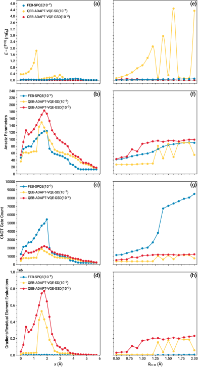
Figure S26: Errors relative to FCI [(a) and (e)], ansatz parameters [(b) and (f)], CNOT gate counts [(c) and (g)], and gradient/residual element evaluations [(d) and (h)] characterizing the FEB-SPQE, QEB-ADAPT-VQE-SD, and QEB-ADAPT-VQE-GSD simulations of the insertion of Be to $\text{H}_{2}$ (left column) and the symmetric dissociation of the $\text{H}_{6}$ ring (right column) as described by the STO-6G basis.

Although in Fig. 8 we focused on the symmetric dissociations of the linear $\text{BeH}_{2}$ and $\text{H}_{6}$ species, similar remarks can be made for the insertion of Be into $\text{H}_{2}$ and the symmetric dissociation of the $\text{H}_{6}$ ring, considered in the Supplemental Material. Indeed, as illustrated in Fig. S26, FEB-SPQE is practically as accurate as QEB-ADAPT-VQE-GSD while leading to more compact ansätze and requiring orders of magnitude less residual element evaluations than gradient element measurements in QEB-ADAPT-VQE-GSD. It is also interesting to note that, even though FEB-SPQE gives rise to quantum circuits containing, in general, a larger number of CNOT gates, as one moves toward the reactants in the reaction pathway of $\text{BeH}_{2}$, FEB-SPQE requires less CNOTs than QEB-ADAPT-VQE-GSD and, eventually, QEB-ADAPT-VQE-SD.

The above analysis demonstrates that FEB-SPQE is an attractive alternative to QEB-ADAPT-VQE-GSD, as it generates the similar energies, closely reproducing those obtained from the exact, FCI, Hamiltonian diagonalizations, while requiring fewer ansatz parameters. Although FEB-SPQE typically requires longer circuits, containing as much as 6–7 times more CNOT gates, the runs are much shorter due to the fact that FEB-SPQE needs a few orders of magnitude less residual element evaluations than gradient element measurements in QEB-ADAPT-VQE-GSD.

IV Conclusions

In this work, we generalized the CNOT-efficient quantum circuits for single and double excitations of Ref. [41] to operators of arbitrary many-body ranks. We demonstrated that, although the FEB/QEB quantum circuits performing $n$-tuple fermionic/qubit excitations still contain a number of CNOT gates that scales exponentially with the excitation rank $n$, they are much more economical than their conventional counterparts. For a given $n$-tuple excitation operator, the FEB scheme will typically require more CNOT gates than QEB, needed to encode the proper fermionic sign. Nevertheless, we showed that the relative difference between the FEB and QEB CNOT counts is decreased as the many-body rank $n$ increases.

Utilizing these CNOT-efficient quantum circuits, we introduced the FEB and QEB variants of SPQE, a hybrid quantum–classical approach that relies on a complete operator pool of particle–hole excitations to iteratively construct the ansatz. By performing numerical simulations for small molecular systems, we demonstrated that FEB- and QEB-SPQE dramatically reduce the CNOT counts relative to their standard counterparts, typically requiring about 6–15 times less CNOTs. We also found that the remarkable savings in terms of CNOTs offered by the FEB and QEB versions of SPQE are even more pronounced in situations involving stronger many-electron correlation effects, which is an encouraging behavior.

When comparing the FEB and QEB variants of SPQE among themselves, we found that the FEB-SPQE scheme offered the best balance between accuracy and computational resources. According to our numerical simulations, while both FEB- and QEB-SPQE produced energies that closely followed those resulting from FCI, FEB-SPQE gave rise to more compact ansätze whose implementation typically required less CNOT gates than QEB-SPQE. This was particularly true at the strong correlation regime, with QEB-SPQE requiring up to 2–3 times more CNOTs than its FEB analog.

Finally, we compared the performance of FEB-SPQE and QEB-ADAPT-VQE, the best SPQE and ADAPT-VQE flavors considered in this study. We showed that both FEB-SPQE and QEB-ADAPT-VQE-GSD provide energies well within chemical accuracy, with the latter being more accurate in the presence of strong correlations. We found that, although FEB-SPQE provided more compact ansätze than QEB-ADAPT-VQE-GSD and required orders of magnitude less residual element evaluations than gradient element measurements in QEB-ADAPT-VQE-GSD, it required many more CNOT gates. Nevertheless, we demonstrated that the replacement of the traditional quantum circuits by their CNOT-efficient analogs resulted in a dramatic decrease in the disparity between the SPQE and ADAPT-VQE CNOT counts.

The colossal decrease in the CNOT counts afforded by the FEB variant of SPQE is certainly remarkable. Nevertheless, the experimental realization of SPQE on NISQ hardware requires even fewer numbers of CNOT gates. In the future work, we will explore various avenues, on top of the FEB and QEB formalisms, to improve the CNOT-efficiency of SPQE. One such option is to combine FEB-/QEB-SPQE with the qubit tapering procedure of Refs. [62, 63], where one takes advantage of $\mathbb{Z}_{2}$ symmetries in the Hamiltonian to eliminate redundant qubits from the simulations. An advantage of qubit tapering is that it does not introduce any approximations, as was the case with the FEB/QEB representations of standard fermionic/qubit quantum circuits. Another possibility is to limit the incorporation of the higher-rank excitation operators in the ansatz, since they are the most demanding in terms of CNOTs. This can be accomplished, for example, by using a more relaxed cumulative threshold value or adding a penalty in the selection criterion that is proportional to the number of CNOT gates of a given operator. To still incorporate the physics associated with the missing important higher-rank excitation operators, a non-iterative energy correction based on the moments of CC equations [64, 65, 66] could be considered. An alternative strategy geared towards more CNOT-efficient FEB-/QEB-SPQE variants is to use an entirely different operator pool. Following the ADAPT-VQE paradigm, of particular interest in this direction is a pool of generalized singles and doubles, whose quantum circuit representations contain a substantially smaller number of CNOT gates compared to those of $n$-tuple particle–hole excitations in conventional SPQE.

APPENDIX A: Selected Projective Quantum Eigensolver

In this appendix, we summarize the salient features of the SPQE algorithm, which serves as a testing ground for illustrating the benefits of the CNOT-efficient FEB/QEB quantum circuits discussed in the previous sections. In particular, we focus on applications of SPQE to electronic structure theory and refer the interested reader to Ref. [17] for the additional details.

PQE is a hybrid quantum–classical approach for optimizing the parameters of a trial state, Eq. (3). In typical applications to quantum chemistry, the reference state $\ket*{\Phi}$ is a single Slater determinant, usually the HF determinant, that can be easily realized on a quantum computer and the unitary operator $U(\mathbf{t})$ is, in general, a UCC unitary, Eq. (7). Similar to conventional CC theory, in PQE we obtain the optimum parameters defining the ground-electronic state and associated energy of a given system by solving the many-electron Schrödinger equation projectively, Eq. (6). The exact eigenstate $\ket*{\Psi_{0}}$ and energy $E_{0}$ can be obtained by employing a full UCC unitary and enforcing the residual condition Eq. (6) for all excited Slater determinants $\ket*{\Phi_{\mu}}$ afforded by the one-electron basis. In practice, however, one utilizes an incomplete operator pool and, thus, Eq. (6) can only be satisfied for the subset of Slater determinants $R=\{\ket*{\Phi_{\mu}}:\kappa_{\mu}\ket*{\Phi}=\ket*{\Phi_{\mu}}\}$, giving rise to an approximate energy $E_{\text{PQE}}(\mathbf{t})>E_{0}$ [see Eq. (4)].

A crucial step in the PQE algorithm is the evaluation of the residual elements $r_{\mu}(\mathbf{t})$, whose number equals that of the excitation operators defining a given UCC ansatz. Since computing the UCC residuals on a classical machine is intractable, we leverage a quantum computer to measure the residual elements. Our group has recently demonstrated how to efficiently evaluate the exact residuals $r_{\mu}(\mathbf{t})$, which are off-diagonal matrix elements of the UCC similarity-transformed Hamiltonian $\bar{H}(\mathbf{t})\equiv U^{\dagger}(\mathbf{t})HU(\mathbf{t})$, as linear combinations of expectation values of $\bar{H}(\mathbf{t})$ with respect to states that can be easily prepared on a quantum device [17]. Indeed, taking advantage of the fact that

$$\ket*{\Omega_{\mu}(\theta)}=e^{\theta\kappa_{\mu}}\ket*{\Phi}=\cos(\theta)\ket*{\Phi}+\sin(\theta)\ket*{\Phi_{\mu}},$$ (A.1)

and that the wavefunction is real, the exact residual element $r_{\mu}(\mathbf{t})$ can be expressed as

$$\begin{split}r_{\mu}(\mathbf{t})=&\expectationvalue*{\bar{H}(\mathbf{t})}{\Omega_{\mu}(\frac{\pi}{4})}\\ &-\frac{1}{2}\left(\expectationvalue*{\bar{H}(\mathbf{t})}{\Phi_{\mu}}+\expectationvalue*{\bar{H}(\mathbf{t})}{\Phi}\right).\end{split}$$ (A.2)

Since the $\expectationvalue*{\bar{H}(\mathbf{t})}{\Phi}$ quantity needs to be computed only once per PQE iteration, the computation of an exact residual element requires the evaluation of only two energy expectation values, i.e., it has a comparable cost to the measurement of an exact gradient element in VQE via the shift rule [67, 68]. After measuring on the quantum device the residuals corresponding to the operators defining the UCC unitary, a classical computer is used to update the optimization parameters,

$$t_{\mu}^{(n+1)}=t_{\mu}^{(n)}+\frac{r_{\mu}^{(n)}(\mathbf{t})}{\Delta_{\mu}},$$ (A.3)

where the superscripts “($n$)” and “($n+1$)” denote quantities at iterations $n$ and $n+1$, respectively, and $\Delta_{\mu}\equiv\Delta_{i_{1}\ldots i_{n}}^{a_{1}\ldots a_{n}}=\epsilon_{i_{1}}+\cdots+\epsilon_{i_{n}}-\epsilon_{a_{1}}-\cdots-\epsilon_{a_{n}}$ are Møller–Plesset denominators with $\epsilon_{p}$ being the HF energy of the $p^{\text{th}}$ spinorbital (see Ref. [17] for the details).

The PQE algorithm described thus far pertains to fixed UCC ansätze, meaning UCC unitaries defined using a constant number of excitation operators. The most widely used procedure for constructing such approaches is to incorporate into the UCC unitary all operators up to a given excitation rank, giving rise to the UCCSD (UCC with singles and doubles), UCCSDT (UCC with singles, doubles, and triples), UCCSDTQ (UCC with singles, doubles, triples, and quadruples), etc. hierarchy of methods that systematically converges to the exact, FCI, solution. Although in the weakly correlated regime the basic UCCSD approach might be enough to obtain energetics within chemical accuracy, as one approaches the strong correlation limit the importance of higher–than–two-body excitations is anticipated to gradually increase. In such situations, higher-level approaches, e.g., UCCSDT, UCCSDTQ, etc., need to be employed. However, due to the inherent rigidity of fixed ansätze, one also introduces a number of superfluous excitation operators that unnecessarily increase the computational cost.

This issue can be remedied by adopting ansätze that are iteratively constructed by selecting operators from a given operator pool based on some importance criterion. Such schemes have been widely employed in computational chemistry in the form of various selected CI approaches [69, 70, 71, 72] and CI/CC quantum Monte Carlo methods [73, 74]. In the realm of quantum computing, the first such adaptive approach was ADAPT-VQE [47], which utilized an operator pool of singles and doubles or their generalized version and a selection criterion based on the magnitude of the individual gradient elements. To ensure that the resulting ADAPT-VQE state would eventually converge to the exact, FCI, solution, the operator pool was not allowed to “drain”, meaning that a given operator could be selected multiple times. Recently, our group has generalized the PQE approach to a flexible, iteratively constructed, ansatz, giving rise to the SPQE scheme. In contrast to ADAPT-VQE, the SPQE method employs a full operator pool, i.e., containing up to $N$-tuple particle–hole excitations with $N$ being the number of correlated electrons, and an importance criterion based on the residuals. According to the Gershgorin circle theorem, the error of the PQE energy with respect to FCI is bound by the sum of the absolute value of the residuals corresponding to operators not included in the ansatz, $\absolutevalue{E_{\text{PQE}}(\mathbf{t})-E_{0}}\leq\sum_{\nu}\absolutevalue{r_{\nu}(\mathbf{t})}$. Thus, by incorporating in the ansatz the operator corresponding to the residual element with the largest magnitude and solving the new set of PQE equations, one reduces the error bound by the largest amount. This is the main philosophy behind the SPQE methodology.

In principle, one could use Eq. (A.2) to compute all residuals corresponding to operators not included in the ansatz. However, a much more efficient way is to extract these residuals from repeated measurements of a single, suitably prepared, state on a quantum device. Ideally, one would prepare and measure the state $\ket*{r(\mathbf{t})}=U^{\dagger}(\mathbf{t})HU(\mathbf{t})\ket*{\Phi}$, but this involves applying the non-unitary Hamiltonian operator $H$. This can be circumvented by replacing the Hamiltonian by the time evolution operator $e^{i\Delta tH}$ and using a small time step $\Delta t$ so that the contributions of non-linear terms become negligible,

$$\begin{split}\ket*{\tilde{r}(\mathbf{t})}=&U^{\dagger}(\mathbf{t})e^{i\Delta tH}U(\mathbf{t})\ket*{\Phi}\\ =&\ket*{\Phi}+i\Delta tU^{\dagger}(\mathbf{t})HU(\mathbf{t})\ket*{\Phi}+\mathcal{O}(\Delta t^{2})\\ =&[1+i\Delta tE_{\text{PQE}}(\mathbf{t})]\ket*{\Phi}\\ &+i\Delta t\sum_{\nu}r_{\nu}(\mathbf{t})\ket*{\Phi_{\nu}}+\mathcal{O}(\Delta t^{2}).\end{split}$$ (A.4)

Using the fact that, independently of the fermionic encoding, there is a one-to-one correspondence between Slater determinants and elements of the computational basis, one can estimate the desired residuals by performing a sufficiently large number of measurements $M$ of identically prepared $\ket*{\tilde{r}}$ states,

$$\absolutevalue{r_{\nu}}^{2}\approx\frac{1}{\Delta t^{2}}\frac{M_{\nu}}{M},$$ (A.5)

where $M_{\nu}$ is the number of times the state $\ket*{\Phi_{\nu}}$ was obtained.

After evaluating the residuals corresponding to operators not included in the current ansatz, the SPQE algorithm proceeds to the next step, namely, the selection of important missing excitations. In contrast to typical ADAPT-VQE applications where the ansatz is expanded one operator per macro-iteration, in SPQE we rely on a cumulative importance criterion, allowing us to add multiple operators at a time, thus accelerating convergence. To be precise, the operators are ordered in ascending order according to $\absolutevalue{r_{\nu}}^{2}$, Eq. (A.5), and, starting from the first element, we keep discarding operators until the following relation is satisfied:

$$\sum_{\text{ discarded}}\absolutevalue{r_{\nu}}^{2}\leq\Omega^{2},$$ (A.6)

where $\Omega^{2}$ is a user-defined threshold. The remaining set of excitation operators are added to the ansatz in order of decreasing $\absolutevalue{r_{\nu}}^{2}$. By appending to the ansatz a batch of operators at a time, SPQE simulations typically converge after a few macro-iterations, dramatically reducing the number of residual element evaluations, while still producing compact ansätze.

APPENDIX B: Computational Details

The CNOT-efficient FEB and QEB quantum circuits performing respectively fermionic and qubit excitations of arbitrary order, along with the standard circuits for qubit excitations, have been implemented in a local version of the QForte package [75]. To gauge the extent to which the FEB and QEB quantum circuits reduce the number of CNOT gates compared to their standard analogs, in particular when higher-than-double excitations are involved, we performed a series of SPQE classical numerical simulations for small molecular systems using a full particle–hole excitation operator pool. To ensure the importance of higher–than–two-body excitations, we studied molecular processes in which the strength of the many-electron correlation effects can be continuously varied from weak to strong. Specifically, we examined the symmetric dissociations of the linear $\text{BeH}_{2}$ and $\text{H}_{6}$ systems, both treated with the minimum STO-6G basis [76] and correlating all electrons. In the computations for $\text{BeH}_{2}$, we employed the grid of Be–H internuclear distances $0.5R_{e}$, $0.6R_{e}$, …, $2.5R_{e}$, where $R_{e}=$1.310\,011\text{\,}\AA$$ is the FCI/STO-6G equilibrium distance. The potential energy curves characterizing the symmetric dissociation of the $\text{H}_{6}$ linear chain were determined using the following uniform grid of distances between neighboring hydrogen atoms, $R_{\text{H--H}}$: 0.5, 0.6, …, $2.0\text{\,}\AA$. In the Supplemental Material, we considered two additional processes, namely, the insertion of Be into $\text{H}_{2}$ and the symmetric dissociation of the $\text{H}_{6}$ ring. As was the case with the computations of their linear counterparts, we employed the STO-6G basis set and correlated all electrons. The reaction pathway defining the insertion of Be into $\text{H}_{2}$ was constructed as follows. We first optimized the geometries of the reactants, $\text{Be}+\text{H}_{2}$, and the product, $\text{BeH}_{2}$, at the FCI/STO-6G level of theory. Following the strategy of Ref. [28], we kept the Be atom fixed at the center of a two-dimensional coordinate system and used the optimized structures to define the lines on which the two H atoms move during the insertion reaction, namely,

$$y(x)=\pm(0.164183x-1.310011),$$ (B.1)

where the $x$ coordinate takes values between $0\text{\,}\AA$ (product, $\text{BeH}_{2}$) and $5.746\,708\text{\,}\AA$ (reactant, $\text{Be}+\text{H}_{2}$). Finally, starting from the optimized geometry of the product, we sampled the reaction coordinate by selecting 30 points with $x$ coordinates given by $x_{n}(\mathrm{\AA})=\frac{5.746708}{29}n$, $n=0,1,\ldots,29$. In the case of the dissociation of the $\text{H}_{6}$ ring, we employed the same grid of H–H internuclear separations as in its linear counterpart.

All SPQE simulations performed in this study utilized a full particle–hole excitation operator pool, i.e., containing up to hextuple excitations for both the $\text{BeH}_{2}$ and $\text{H}_{6}$ systems. We considered two values of the parameter $\Omega$ defining the cumulative importance criterion, Eq. (A.6), namely, ${10}^{-1}\text{\,}\textit{E}_{\mathrm{h}}$ and ${10}^{-2}\text{\,}\textit{E}_{\mathrm{h}}$ (results for the former case are reported in the Supplemental Material). All PQE calculations employed a micro-iteration threshold of ${10}^{-5}\text{\,}\textit{E}_{\mathrm{h}}$ for the residual norm $\norm{\mathbf{r}}$ and the DIIS approach was utilized to accelerate convergence. Typically, the PQE cycles of an SPQE computation converged within 10 to 20 micro-iterations, although there were a few exceptions requiring a far greater number. Consequently, in order to maintain a relatively low count of residual element evaluations, the maximum number of micro-iterations was set to 50.

For each of the systems examined in this study, we also carried out ADAPT-VQE simulations using two kinds of operator pools, namely, single and double particle–hole excitations and generalized singles and doubles. As is typically done in ADAPT-VQE, a single operator was added to the ansatz per macro-iteration and the pool was not allowed to “drain”. For each operator pool, we performed two sets of calculations employing the macro-iteration gradient thresholds of ${10}^{-2}\text{\,}\textit{E}_{\mathrm{h}}$ and ${10}^{-3}\text{\,}\textit{E}_{\mathrm{h}}$ (with results for the former being reported in the Supplemental Material). All VQE computations utilized the Broyden–Fletcher–Goldfarb–Shanno (BFGS) optimizer [77, 78, 79, 80], as implemented in SCIPY [81], and a micro-iteration convergence criterion of ${10}^{-5}\text{\,}\textit{E}_{\mathrm{h}}$ for the gradient norm $\norm{\mathbf{g}}$. In general, the VQE cycles of an ADAPT-VQE simulation required many micro-iterations to achieve convergence. Thus, as was the case with the SPQE calculations, the maximum number of micro-iterations was set to 50 to reduce the number of gradient evaluations.

All correlated approaches were based on RHF references with the one- and two-electron integrals obtained with Psi4 [82].

This Supplemental Material document is organized as follows. In Sec. SI we describe how to decompose the multi-qubit-controlled $R_{y}(2\theta)$ gate, which is needed to define the CNOT-efficient quantum circuits of Figs. 4 and 5 in the main text, in terms of single- and two-qubit gates. In Sec. SII, we contemplate the use of circuit identities for the removal of a single CNOT gate from the quantum circuits of Figs. 4 and 5 in the main text. Section SIII provides, in a graphical form, the results of our additional numerical simulations. In particular, in Sec. SIII.1 we compare the convergence to the exact, full configuration interaction (FCI), solution of the fermionic-excitation-based (FEB) and qubit-excitation-based (QEB) flavors of UCCSD, UCCSDT, and UCCSDTQ for the symmetric dissociation of the linear $\text{H}_{6}$/STO-6G system. In Sec. SIII.2 we compare the CNOT counts obtained with SPQE and FEB-SPQE and with qSPQE and QEB-SPQE for the symmetric dissociations of the linear $\text{BeH}_{2}$ and $\text{H}_{6}$ systems, the symmetric dissociation of the $\text{H}_{6}$ ring, and the insertion of Be into $\text{H}_{2}$, as described by the STO-6G basis. In the cases of the symmetric dissociation of the $\text{H}_{6}$ ring and the insertion of Be into $\text{H}_{2}$, we also include the pertinent results obtained with the tighter $\Omega=${10}^{-2}\text{\,}\textit{E}_{\mathrm{h}}$$ threshold. In Sec. SIII.3 we compare the efficiency of the FEB and QEB variants of SPQE for the symmetric dissociations of the linear $\text{BeH}_{2}$ and $\text{H}_{6}$ systems, the symmetric dissociation of the $\text{H}_{6}$ ring, and the insertion of Be into $\text{H}_{2}$, as described by the STO-6G basis. In the cases of the symmetric dissociation of the $\text{H}_{6}$ ring and the insertion of Be into $\text{H}_{2}$, we also examine the performance of FEB- and QEB-SPQE. In Sec. SIII.4, we compare the efficiency of the FEB and QEB variants of ADAPT-VQE for the symmetric dissociations of the linear $\text{BeH}_{2}$ and $\text{H}_{6}$ systems, the symmetric dissociation of the $\text{H}_{6}$ ring, and the insertion of Be into $\text{H}_{2}$, as described by the STO-6G basis. We examined two operator pools, namely, particle–hole singles and doubles and their generalized extension, and two convergence criteria, namely, $10^{-2}$ and ${10}^{-3}\text{\,}\textit{E}_{\mathrm{h}}$. Finally, in Sec. SIII.5, we compare the performance of FEB-SPQE with that of QEB-ADAPT-VQE-SD and its GSD variant for the symmetric dissociation of the $\text{H}_{6}$ ring and the insertion of Be into $\text{H}_{2}$, as described by the STO-6G basis.

SI Decomposition of Multi-Qubit-Controlled $\boldsymbol{R_{y}(2\theta)}$ Gate

Before we outline how to decompose a general multi-qubit-controlled $R_{y}(2\theta)$ gate, we begin with the simpler case of an $R_{y}(2\theta)$ rotation controlled on a single qubit. As shown in Refs. [55, 56, 41] of the main text and Fig. S1, there are multiple ways of expressing a controlled $R_{y}(2\theta)$ rotation in terms of single- and two-qubit gates. What is common in all of these circuits is that the controlled $R_{y}(2\theta)$ gate is replaced by two half-way rotations of opposite directions, $R_{y}(\theta)$ and $R_{y}(-\theta)$, and two two-qubit gates, either CNOTs or CZs. There are two possible arrangements of the gates in the resulting circuits, namely, $R_{y}(\theta)\rightarrow\text{TQG}\rightarrow R_{y}(-\theta)\rightarrow\text{TQG}$ and $\text{TQG}\rightarrow R_{y}(-\theta)\rightarrow\text{TQG}\rightarrow R_{y}(\theta)$, with TQG being either CNOT or CZ. We will refer to these arrangements as “forward”/“backward” since a two-qubit gate is placed after/before each $R_{y}$ rotation. Note that the CNOT gates appearing in Fig. S1 are controlled on the bottom qubit, as is the case with the controlled $R_{y}(2\theta)$ gate. Nevertheless, the flexibility in transforming a CZ gate to a CNOT, as shown in Fig. S2, allows one to construct additional equivalent circuits where the CNOT gates are controlled on the top qubit. In the case of an anti-controlled $R_{y}(2\theta)$ gate, there are two families of decompositions. The first one, shown in Fig. S3, relies on anti-CNOT/anti-CZ gates. In the second family of decompositions, using the circuit identity shown in Fig. S4, the anti-controlled $R_{y}(2\theta)$ gate is transformed to its controlled analog and its decomposition proceeds as in Fig. S1.

Figure S1: Decomposition of controlled $R_{y}(2\theta)$ gate in terms of single-qubit $R_{y}(\theta)$ and $R_{y}(-\theta)$ rotations and two-qubit CNOT/CZ gates.

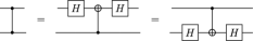
Figure S2: Transformation of a CZ gate into a CNOT.

Figure S3: Decomposition of anti-controlled $R_{y}(2\theta)$ gate in terms of single-qubit $R_{y}(\theta)$ and $R_{y}(-\theta)$ rotations and two-qubit anti-CNOT/anti-CZ gates.

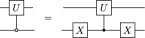
Figure S4: Transformation of an anti-controlled gate into its controlled counterpart.

The decomposition of a multi-qubit-controlled $R_{y}(2\theta)$ gate is accomplished by applying the identities in Figs. S1 and S3 one (anti-)control qubit at a time (see, for example, Ref. [41] of the main text). For example, given an $n$-qubit-controlled $R_{y}(2\theta)$ gate, we start by selecting one of the (anti-)control qubits. After the first decomposition, we end up with 2 ($n-1$)-qubit-controlled $R_{y}$ gates, with angles $\theta$ and $-\theta$, and 2 two-qubit gates. In the next step, we choose another (anti-)control qubit and decompose both of the ($n-1$)-qubit-controlled $R_{y}$ gates. After the second decomposition, the circuit contains 4 ($n-2$)-qubit-controlled $R_{y}$ rotations, 2 with angle $\tfrac{\theta}{2}$ and 2 with angle $-\tfrac{\theta}{2}$, and 6 two-qubit gates. After repeating this procedure for all remaining (anti-)control qubits, the final quantum circuit will contain $2^{n}$ single-qubit $R_{y}$ rotations, half with angle $\tfrac{\theta}{2^{n-1}}$ and half with angle $-\tfrac{\theta}{2^{n-1}}$, and $2^{n+1}-2$ two-qubit gates. In the optimum implementation, one decomposes the multi-qubit-controlled $R_{y}$ rotations in a way that maximizes the number of adjacent equivalent two-qubit gates. This can be accomplished by alternating the “forward” and “backward” arrangements of decomposed multi-qubit-controlled $R_{y}$ rotations. By doing so, one cancels adjacent equivalent two-qubit gates, reducing their total number to $2^{n-1}$. In Fig. S5, we illustrate the aforementioned procedure in the case of the multi-qubit-controlled $R_{y}(2\theta)$ gate appearing in the definition of FEB/QEB double excitations.

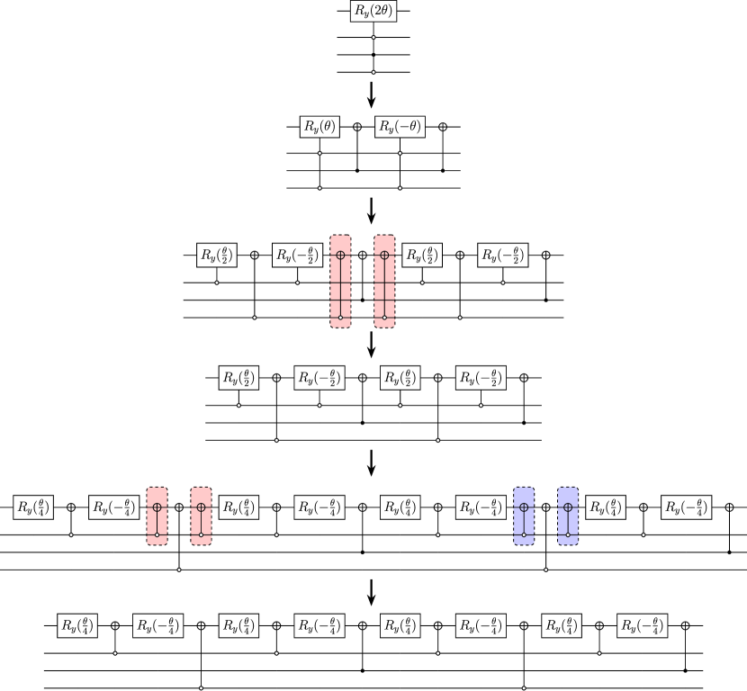
Figure S5: Decomposition of multi-qubit-controlled $R_{y}(2\theta)$ gate appearing in the definition of FEB/QEB double excitations. CNOT gates shaded with the same color cancel out.

SII On the Use of Circuit Identities for the Removal of a Single CNOT Gate

In Ref. [41] of the main text, Yordanov et al. demonstrated how to reduce the CNOT counts of the FEB and QEB quantum circuits by a single CNOT gate. The circuit identity behind this reduction is shown in Fig. S6 and it involves the replacement of the product of a CZ gate times a CNOT by a single CNOT gate and five single-qubit ones. To take advantage of this circuit identity, the following procedure is typically employed. In the initial step, one uses the circuit identity of Fig. S4 to replace all anti-control qubits of the multi-qubit-controlled $R_{y}(2\theta)$ gate by control ones. Subsequently, one decomposes the multi-qubit-controlled $R_{y}(2\theta)$ gate into a series of alternating $R_{y}$ rotations and CZ gates, similarly to the procedure outlined in Fig. S5; note that the use of CZ gates rather than CNOTs is crucial for eliminating a CNOT gate. In the next step, one uses the circuit identity of Fig. S6 to replace the right-most CZ gate and one of the CNOTs immediately after the multi-qubit-controlled $R_{y}(2\theta)$ gate by a single CNOT and five single-qubit gates. Depending on which two-qubit gates are directly available in a given hardware implementation, a final step might be involved in which the remaining CZ gates are transformed into CNOTs using the circuit identity of Fig. S2. An illustration of the above procedure can be found in Fig. S7, using as an example the QEB quantum circuit performing a double qubit excitation.

As already mentioned, depending on the native gate set available on the hardware, one might need to replace all CZ gates by CNOTs. However, by doing so one introduces a number of Hadamard gates that scales linearly with the excitation rank $n$. To be precise, the number of required Hadamard gates is $4n-2$. In total, the number of single-qubit gates increases by $4(n+1)$ when applying the identity responsible for eliminating a single CNOT. Therefore, as the excitation rank increases, the gate errors associated with the aforementioned single-qubit gates are anticipated to outweigh the benefits of removing a single CNOT.

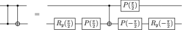
Figure S6: Circuit identity that replaces the product of a CZ and a CNOT gate by a circuit containing a single CNOT and single-qubit gates. Note that $P(\theta)\equiv\big{(}\begin{smallmatrix}1&0\\ 0&e^{i\theta}\end{smallmatrix}\big{)}$ is the phase shift gate.

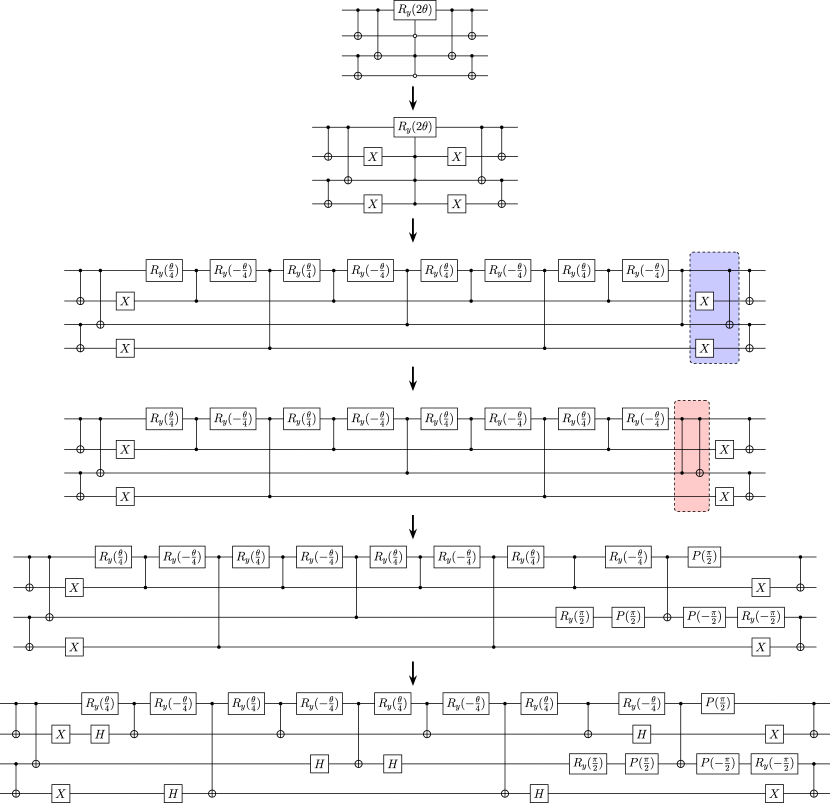
Figure S7: Illustration of the process that reduces the number of CNOT gates by 1, using the QEB circuit that performs double qubit excitations as an example. The gates shaded in blue color commute. The circuit identity of Fig. S6 is applied to the gates shaded in red color. Note that $P(\theta)\equiv\big{(}\begin{smallmatrix}1&0\\ 0&e^{i\theta}\end{smallmatrix}\big{)}$ is the phase shift gate.

SIII Results of Additional Numerical Simulations

SIII.1 Convergence to FCI of QEB-UCCSD, QEB-UCCSDT, and QEB-UCCSDTQ

SIII.2 Standard vs CNOT-Efficient SPQE

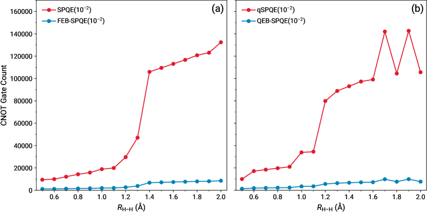
Figure S14: Total CNOT gate counts characterizing the (a) fermionic SPQE and FEB-SPQE and (b) qubit qSPQE and QEB-SPQE ansatz unitaries for the symmetric dissociation of the $\text{H}_{6}$/STO-6G ring. All computations employ a selection threshold of $\Omega=${10}^{-2}\text{\,}\textit{E}_{\mathrm{h}}$$.

SIII.3 FEB-SPQE vs QEB-SPQE

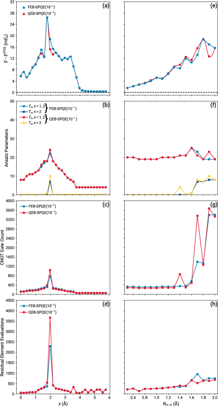
Figure S16: Errors relative to FCI [(a) and (e)], ansatz parameters [(b) and (f)], CNOT gate counts [(c) and (g)], and residual element evaluations [(d) and (h)] characterizing the FEB- and QEB-SPQE simulations of the insertion of Be to $\text{H}_{2}$ (left column) and the symmetric dissociation of the $\text{H}_{6}$ ring (right column) as described by the STO-6G basis.

SIII.4 FEB-ADAPT-VQE vs QEB-ADAPT-VQE

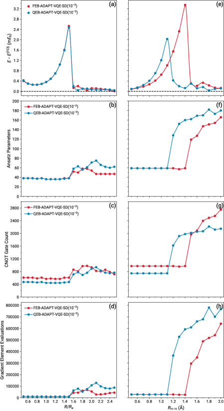
Figure S19: Errors relative to FCI [(a) and (e)], ansatz parameters [(b) and (f)], CNOT gate counts [(c) and (g)], and gradient element evaluations [(d) and (h)] characterizing the FEB- and QEB-ADAPT-VQE-SD simulations of the symmetric dissociations of the linear $\text{BeH}_{2}$ (left column) and $\text{H}_{6}$ (right column) systems as described by the STO-6G basis.

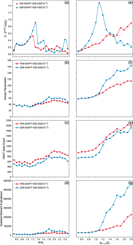
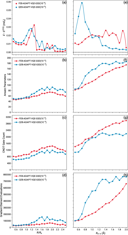
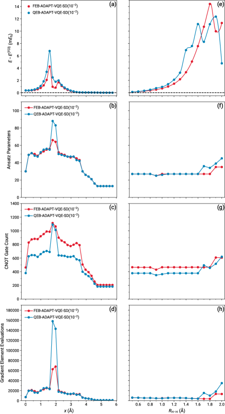
Figure S20: Errors relative to FCI [(a) and (e)], ansatz parameters [(b) and (f)], CNOT gate counts [(c) and (g)], and gradient element evaluations [(d) and (h)] characterizing the FEB- and QEB-ADAPT-VQE-GSD simulations of the symmetric dissociations of the linear $\text{BeH}_{2}$ (left column) and $\text{H}_{6}$ (right column) systems as described by the STO-6G basis.

Figure S21: Errors relative to FCI [(a) and (e)], ansatz parameters [(b) and (f)], CNOT gate counts [(c) and (g)], and gradient element evaluations [(d) and (h)] characterizing the FEB- and QEB-ADAPT-VQE-GSD simulations of the symmetric dissociations of the linear $\text{BeH}_{2}$ (left column) and $\text{H}_{6}$ (right column) systems as described by the STO-6G basis.

Figure S22: Errors relative to FCI [(a) and (e)], ansatz parameters [(b) and (f)], CNOT gate counts [(c) and (g)], and gradient element evaluations [(d) and (h)] characterizing the FEB- and QEB-ADAPT-VQE-SD simulations of the insertion of Be to $\text{H}_{2}$ (left column) and the symmetric dissociation of the $\text{H}_{6}$ ring (right column) as described by the STO-6G basis.

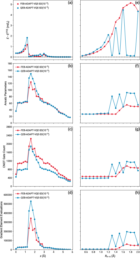
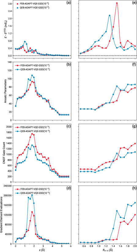
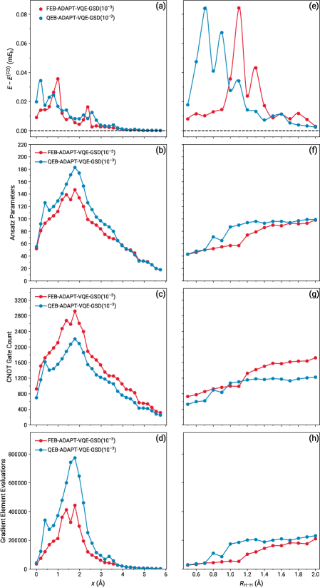
Figure S23: Errors relative to FCI [(a) and (e)], ansatz parameters [(b) and (f)], CNOT gate counts [(c) and (g)], and gradient element evaluations [(d) and (h)] characterizing the FEB- and QEB-ADAPT-VQE-SD simulations of the insertion of Be to $\text{H}_{2}$ (left column) and the symmetric dissociation of the $\text{H}_{6}$ ring (right column) as described by the STO-6G basis.

Figure S24: Errors relative to FCI [(a) and (e)], ansatz parameters [(b) and (f)], CNOT gate counts [(c) and (g)], and gradient element evaluations [(d) and (h)] characterizing the FEB- and QEB-ADAPT-VQE-GSD simulations of the insertion of Be to $\text{H}_{2}$ (left column) and the symmetric dissociation of the $\text{H}_{6}$ ring (right column) as described by the STO-6G basis.

Figure S25: Errors relative to FCI [(a) and (e)], ansatz parameters [(b) and (f)], CNOT gate counts [(c) and (g)], and gradient element evaluations [(d) and (h)] characterizing the FEB- and QEB-ADAPT-VQE-GSD simulations of the insertion of Be to $\text{H}_{2}$ (left column) and the symmetric dissociation of the $\text{H}_{6}$ ring (right column) as described by the STO-6G basis.

SIII.5 FEB-SPQE vs QEB-ADAPT-VQE

References

- Benioff [1980] P. Benioff, The computer as a physical system: A microscopic quantum mechanical Hamiltonian model of computers as represented by Turing machines, J. Stat. Phys. 22, 563 (1980).
- Manin [1980] Y. I. Manin, Computable and Uncomputable [in Russian] (Sovetskoye Radio, Moscow, 1980) see Mathematics as Metaphor: Selected Essays of Yuri I. Manin (Americal Mathematical Society, Providence, 2007), pp. 77–78 for an English translation.
- Feynman [1982] R. P. Feynman, Simulating physics with computers, Int. J. Theor. Phys. 21, 467 (1982).
- Preskill [2021] J. Preskill, Quantum computing 40 years later, arXiv:2106.10522v2 [quant-ph] (2021).
- Preskill [2018] J. Preskill, Quantum computing in the NISQ era and beyond, Quantum 2, 79 (2018).
- Roffe [2019] J. Roffe, Quantum error correction: An introductory guide, Contemp. Phys. 60, 226 (2019).
- Haroche and Raimond [1996] S. Haroche and J.-M. Raimond, Quantum computing: Dream or nightmare, Phys. Today 49, 51 (1996).
- Bharti et al. [2022] K. Bharti, A. Cerveta-Lierta, T. H. Kyaw, T. Haug, S. Alperin-Lea, A. Anand, M. Degroote, H. Heimonen, J. S. Kottmann, T. Menke, W.-K. Mok, S. Sim, L.-C. Kwek, and A. Aspuru-Guzik, Noisy intermediate-scale quantum algorithms, Rev. Mod. Phys. 94, 015004 (2022).
- Kitaev [1995] A. Y. Kitaev, Quantum measurements and the abelian stabilizer problem, arXiv:9511026 [quant-ph] (1995).
- Abrams and Lloyd [1997] D. S. Abrams and S. Lloyd, Simulation of many-body Fermi systems on a universal quantum computer, Phys. Rev. Lett. 79, 2586 (1997).
- Abrams and Lloyd [1999] D. S. Abrams and S. Lloyd, Quantum algorithm providing exponential speed increase for finding eigenvalues and eigenvectors, Phys. Rev. Lett. 83, 5162 (1999).
- Peruzzo et al. [2014] A. Peruzzo, J. McClean, P. Shadbolt, M.-H. Yung, X.-Q. Zhou, P. J. Love, A. Aspuru-Guzik, and J. L. O’Brien, A variational eigenvalue solver on a photonic quantum processor, Nat. Commun. 5, 4213 (2014).
- McClean et al. [2016] J. R. McClean, J. Romero, R. Babbush, and A. Aspuru-Guzik, The theory of variational quantum-classical algorithms, New J. Phys. 18, 023023 (2016).
- Cerezo et al. [2021] M. Cerezo, A. Arrasmith, R. Babbush, S. C. Benjamin, S. Endo, K. Fujii, J. R. McClean, K. Mitarai, X. Yuan, L. Cincio, and P. J. Coles, Variational quantum algorithms, Nat. Rev. Phys. 3, 625 (2021).
- Tilly et al. [2021] J. Tilly, H. Chen, S. Cao, D. Picozzi, K. Setia, Y. Li, E. Grant, L. Wossnig, I. Rungger, G. H. Booth, and J. Tennyson, The variational quantum eigensolver: A review of methods and best practices, arXiv:2111.05176 [quant-ph] (2021).
- Fedorov et al. [2022a] D. A. Fedorov, B. Peng, N. Govind, and Y. Alexeev, VQE method: A short survey and recent developments, Mater. Theory 6, 2 (2022a).
- Stair and Evangelista [2021] N. H. Stair and F. A. Evangelista, Simulating many-body systems with a projective quantum eigensolver, PRX Quantum 2, 030301 (2021).
- Smart and Mazziotti [2021] S. E. Smart and D. A. Mazziotti, Quantum solver of contracted eigenvalue equations for scalable molecular simulations on quantum computing devices, Phys. Rev. Lett. 126, 070504 (2021).
- Mazziotti [2006] D. A. Mazziotti, Anti-Hermitian contracted Schrödinger equation: Direct determination of the two-electron reduced density matrices of many-electron molecules, Phys. Rev. Lett. 97, 143002 (2006).
- Kutzelnigg [1977] W. Kutzelnigg, in Methods of Electronic Structure Theory, edited by H. F. Schaefer, III (Springer, Boston, 1977) pp. 129–188.
- Kutzelnigg [1982] W. Kutzelnigg, Quantum chemistry in Fock space. I. The universal wave and energy operators, J. Chem. Phys. 77, 3081 (1982).
- Kutzelnigg and Koch [1983] W. Kutzelnigg and S. Koch, Quantum chemistry in Fock space. II. Effective Hamiltonians in Fock space, J. Chem. Phys. 79, 4315 (1983).
- Kutzelnigg [1984] W. Kutzelnigg, Quantum chemistry in Fock space. III. Particle-hole formalism, J. Chem. Phys. 80, 822 (1984).
- Bartlett et al. [1989] R. J. Bartlett, S. A. Kucharski, and J. Noga, Alternative coupled-cluster ansätze II. The unitary coupled-cluster method, Chem. Phys. Lett. 155, 133 (1989).
- Szalay et al. [1995] P. G. Szalay, M. Nooijen, and R. J. Bartlett, Alternative ansätze in single reference coupled-cluster theory. III. A critical analysis of different methods, J. Chem. Phys. 103, 281 (1995).
- Taube and Bartlett [2006] A. G. Taube and R. J. Bartlett, New perspectives on unitary coupled-cluster theory, Int. J. Quantum Chem. 106, 3393 (2006).
- Cooper and Knowles [2010] B. Cooper and P. J. Knowles, Benchmark studies of variational, unitary and extended coupled cluster methods, J. Chem. Phys. 133, 234102 (2010).
- Evangelista [2011] F. A. Evangelista, Alternative single-reference coupled cluster approaches for multireference problems: The simpler, the better, J. Chem. Phys. 134, 224102 (2011).
- Harsha et al. [2018] G. Harsha, T. Shiozaki, and G. E. Scuseria, On the difference between variational and unitary coupled clutser theories, J. Chem. Phys. 148, 044107 (2018).
- Filip and Thom [2020] M.-A. Filip and A. J. W. Thom, A stochastic approach to unitary coupled cluster, J. Chem. Phys. 153, 214106 (2020).
- Freericks [2022] J. K. Freericks, Operator relationship between conventional coupled cluster and unitary coupled cluster, Symmetry 14, 494 (2022).
- Anand et al. [2022] A. Anand, P. Schleich, S. Alperin-Lea, P. W. K. Jensen, S. Sim, M. Diaz-Tinoco, J. S. Kottmann, M. Degroote, A. F. Izmaylov, and A. Aspuru-Guzik, A quantum computing view on unitary coupled cluster theory, Chem. Soc. Rev. 51, 1659 (2022).
- Coester [1958] F. Coester, Bound states of a many-particle system, Nucl. Phys. 7, 421 (1958).
- Coester and Kümmel [1960] F. Coester and H. Kümmel, Short-range correlations in nuclear wave functions, Nucl. Phys. 17, 477 (1960).
- Čížek [1966] J. Čížek, On the correlation problem in atomic and molecular systems. Calculation of wavefunction components in Ursell-type expansion using quantum-field theoretical methods, J. Chem. Phys. 45, 4256 (1966).
- Čížek [1969] J. Čížek, On the use of the cluster expansion and the technique of diagrams in calculations of correlation effects in atoms and molecules, Adv. Chem. Phys. 14, 35 (1969).
- Čížek and Paldus [1971] J. Čížek and J. Paldus, Correlation problems in atomic and molecular systems III. Rederivation of the coupled-pair many-electron theory using the traditional quantum chemical methods, Int. J. Quantum Chem. 5, 359 (1971).
- Paldus et al. [1972] J. Paldus, J. Čížek, and I. Shavitt, Correlation problems in atomic and molecular systems. IV. Extended coupled-pair many-electron theory and its application to the molecule, Phys. Rev. A 5, 50 (1972).
- Ryabinkin et al. [2018] I. G. Ryabinkin, T.-C. Yen, S. N. Genin, and A. F. Izmaylov, Qubit coupled cluster method: A systematic approach to quantum chemistry on a quantum computer, J. Chem. Theory Comput. 14, 6317 (2018).
- Ryabinkin et al. [2020] I. G. Ryabinkin, R. A. Lang, S. N. Genin, and A. F. Izmaylov, Iterative qubit coupled cluster approach with efficient screening of generators, J. Chem. Theory Comput. 16, 1055 (2020).
- Yordanov et al. [2020] Y. S. Yordanov, D. R. M. Arvidsson-Shukur, and C. H. W. Barnes, Efficient quantum circuits for quantum computational chemistry, Phys. Rev. A 102, 062612 (2020).
- Yordanov et al. [2021] Y. S. Yordanov, V. Armaos, C. H. W. Barnes, and D. R. M. Arvidsson-Shukur, Qubit-excitation-based adaptive variational quantum eigensolver, Commun. Phys. 4, 228 (2021).
- Tang et al. [2021] H. L. Tang, V. O. Shkolnikov, G. S. Barron, H. R. Grimsley, N. J. Mayhall, E. Barnes, and S. E. Economou, Qubit-ADAPT-VQE: An adaptive algorithm for constructing hardware-efficient ansätze on a quantum processor, PRX Quantum 2, 020310 (2021).
- Xia and Kais [2021] R. Xia and S. Kais, Qubit coupled cluster singles and doubles variational quantum eigensolver ansatz for electronic structure calculations, Quantum Sci. Technol. 6, 015001 (2021).
- Mazziotti et al. [2021] D. A. Mazziotti, S. E. Smart, and A. R. Mazziotti, Quantum simulation of molecules without fermionic encoding of the wave function, New J. Phys. 23, 113037 (2021).
- Smart and Mazziotti [2022] S. E. Smart and D. A. Mazziotti, Many-fermion simulation from the contracted quantum eigensolver without fermionic encoding of the wave function, Phys. Rev. A 105, 062424 (2022).
- Grimsley et al. [2019] H. R. Grimsley, S. E. Economou, E. Barnes, and N. J. Mayhall, An adaptive variational algorithm for exact molecular simulations on a quantum computer, Nat Commun. 10, 3007 (2019).
- Fedorov et al. [2022b] D. A. Fedorov, Y. Alexeev, S. K. Gray, and M. J. Otten, Unitary selective coupled-cluster method, Quantum 6, 703 (2022b).
- Nooijen [2000] M. Nooijen, Can the eigenstates of a many-body Hamiltonian be represented exactly using a general two-body cluster expansion?, Phys. Rev. Lett. 84, 2108 (2000).
- Nakatsuji [2000] H. Nakatsuji, Structure of the exact wave function, J. Chem. Phys. 113, 2949 (2000).
- goo [2021] Quantum Computer Datasheet, Google (2021).
- Evangelista et al. [2019] F. A. Evangelista, G. K.-L. Chan, and G. E. Scuseria, Exact parameterization of fermionic wave functions via unitary coupled cluster theory, J. Chem. Phys. 151, 244112 (2019).
- Jordan and Wigner [1928] P. Jordan and E. Wigner, Über das Paulische Äquivalenzverbot, Z. Phys. 47, 631 (1928).
- Romero et al. [2019] J. Romero, R. Babbush, J. R. McClean, C. Hempel, P. J. Love, and A. Aspuru-Guzik, Strategies for quantum computing molecular energies using the unitary coupled cluster ansatz, Quantum Sci. Technol. 4, 014008 (2019).
- Barenco et al. [1995] A. Barenco, C. H. Bennett, R. Cleve, D. P. DiVincenzo, N. Margolus, P. Shor, T. Sleator, J. A. Smolin, and H. Weinfurter, Elementary gates for quantum computation, Phys. Rev. A 52, 3457 (1995).
- Yordanov and Barnes [2019] Y. S. Yordanov and C. H. W. Barnes, Implementation of a general single-qubit positive operator-valued measure on a circuit-based quantum computer, Phys. Rev. A 100, 062317 (2019).
- Yordanov [2021] Y. S. Yordanov, Quantum Computational Chemistry Methods for Early-Stage Quantum Computers, Ph.D. thesis, University of Cambridge (2021).
- Wu and Lidar [2002] L.-A. Wu and D. A. Lidar, Qubits as parafermions, J. Math. Phys. 43, 4506 (2002).
- Pulay [1980] P. Pulay, Convergence acceleration of iterative sequences. The case of SCF iteration, Chem. Phys. Lett. 73, 393 (1980).
- Pulay [1982] P. Pulay, Improved SCF convergence acceleration, J. Comput. Chem. 3, 556 (1982).
- Scuseria et al. [1986] G. E. Scuseria, T. J. Lee, and H. F. Schaefer III, Accelerating the convergence of the coupled-cluster approach, Chem. Phys. Lett. 130, 236 (1986).
- Bravyi et al. [2017] S. Bravyi, J. M. Gambetta, A. Mezzacapo, and K. Temme, Tapering off qubits to simulate fermionic Hamiltonians, arXiv:1701.08213 [quant-ph] (2017).
- Setia et al. [2020] K. Setia, R. Chen, J. E. Rice, A. Mezzacapo, M. Pistoia, and J. D. Whitfield, Reducing qubit requirements for quantum simulations using molecular point group symmetries, J. Chem. Theory Comput. 16, 6091 (2020).
- Jankowski et al. [1991] K. Jankowski, J. Paldus, and P. Piecuch, Method of moments approach and coupled cluster theory, Theor. Chim. Acta 80, 223 (1991).
- Piecuch and Kowalski [2000] P. Piecuch and K. Kowalski, in Computational Chemistry: Reviews of Current Trends, Vol. 5, edited by J. Leszczyński (World Scientific, Singapore, 2000) pp. 1–104.
- Kowalski and Piecuch [2000] K. Kowalski and P. Piecuch, The method of moments of coupled-cluster equations and the renormalized CCSD[T], CCSD(T), CCSD(TQ), and CCSDT(Q) approaches, J. Chem. Phys. 113, 18 (2000).
- Schuld et al. [2019] M. Schuld, V. Bergholm, C. Gogolin, J. Izaac, and N. Killoran, Evaluating analytic gradients on quantum hardware, Phys. Rev. A 99, 032331 (2019).
- Kottmann et al. [2021] J. S. Kottmann, A. Anand, and A. Aspuru-Guzik, A feasible approach for automatically differentiable unitary coupled-cluster on quantum computers, Chem. Sci. 12, 3497 (2021).
- Whitten and Hackmeyer [1969] J. L. Whitten and M. Hackmeyer, Configuration interaction studies of ground and excited states of polyatomic molecules. I. The CI formulation and studies of formaldehyde, J. Chem. Phys. 51, 5584 (1969).
- Bender and Davidson [1969] C. F. Bender and E. R. Davidson, Studies in configuration interaction: The first-row diatomic hydrides, Phys. Rev. 183, 23 (1969).
- Huron et al. [1973] B. Huron, J.-P. Malrieu, and P. Rancurel, Iterative perturbation calculations of ground and excited state energies from multiconfigurational zeroth-order wavefunctions, J. Chem. Phys. 58, 5745 (1973).
- Buenker and Peyerimhoff [1974] R. J. Buenker and S. D. Peyerimhoff, Individualized configuration selection in CI calculations with subsequent energy extrapolation, Theor. Chim. Acta 35, 33 (1974).
- Booth et al. [2009] G. H. Booth, A. J. W. Thom, and A. Alavi, Fermion Monte Carlo without fixed nodes: A game of life, death, and annihilation in Slater determinant space, J. Chem. Phys. 131, 054106 (2009).
- Thom [2010] A. J. W. Thom, Stochastic coupled cluster theory, Phys. Rev. Lett. 105, 263004 (2010).
- Stair and Evangelista [2022] N. H. Stair and F. A. Evangelista, QForte: An efficient state-vector emulator and quantum algorithms library for molecular electronic structure, J. Chem. Theory Comput. 18, 1555 (2022).
- Hehre et al. [1969] W. J. Hehre, R. F. Stewart, and J. A. Pople, Self-consistent molecular-orbital methods. I. Use of Gaussian expansions of Slater-type atomic orbitals, J. Chem. Phys. 51, 2657 (1969).
- Broyden [1970] C. G. Broyden, The convergence of a class of double-rank minimization algorithms: 2. The new algorithm, IMA J. Appl. Math. 6, 222 (1970).
- Fletcher [1970] R. Fletcher, A new approach to variable metric algorithms, Comput. J. 13, 317 (1970).
- Goldfarb [1970] D. Goldfarb, A family of variable-metric methods derived by variational means, Math. Comp. 24, 23 (1970).
- Shanno [1970] D. F. Shanno, Conditioning of quasi-Newton methods for function minimization, Math. Comp. 24, 647 (1970).
- Virtanen et al. [2020] P. Virtanen, R. Gommers, T. E. Oliphant, M. Haberland, T. R. amd D. Cournapeau, E. Burovski, P. Peterson, W. Weckesser, J. Bright, S. J. van der Walt, M. Brett, J. Wilson, K. J. Millman, N. Mayorov, A. R. J. Nelson, E. Jones, R. Kern, E. Larson, C. J. Carey, I. Polat, Y. Feng, E. W. Moore, J. VanderPlas, D. Laxalde, J. Perktold, R. Cimrman, I. Henriksen, E. A. Quintero, C. R. Harris, A. M. Archibald, A. H. Ribeiro, F. Pedregosa, P. van Mulbregt, and SciPy 1.0 Contributors, Scipy 1.0: Fundamental algorithms for scientific computing in python, Nat. Methods 17, 261 (2020).
- Smith et al. [2020] D. G. A. Smith, L. A. Burns, A. C. Simmonett, R. M. Parrish, M. C. Schieber, R. Galvelis, P. Kraus, H. Kruse, R. D. Remigio, A. Alenaizan, A. M. James, S. Lehtola, J. P. Misiewicz, M. Scheurer, R. A. Shaw, J. B. Schriber, Y. Xie, Z. L. Glick, D. A. Sirianni, J. S. O’Brien, J. M. Waldrop, A. Kumar, E. G. Hohenstein, B. P. Pritchard, B. R. Brooks, H. F. Schaefer III, A. Y. Sokolov, K. Patkowski, A. E. DePrince III, U. Bozkaya, R. A. King, F. A. Evangelista, J. M. Turney, T. D. Crawford, and C. D. Sherrill, Psi4 1.4: Open-source software for high-throughput quantum chemistry, J. Chem. Phys. 152, 184108 (2020).
Supplemental Material: