Vote’n’Rank: Revision of Benchmarking with Social Choice Theory

Abstract

The development of state-of-the-art systems in different applied areas of machine learning (ML) is driven by benchmarks, which have shaped the paradigm of evaluating generalisation capabilities from multiple perspectives. Although the paradigm is shifting towards more fine-grained evaluation across diverse tasks, the delicate question of how to aggregate the performances has received particular interest in the community. In general, benchmarks follow the unspoken utilitarian principles, where the systems are ranked based on their mean average score over task-specific metrics. Such aggregation procedure has been viewed as a sub-optimal evaluation protocol, which may have created the illusion of progress. This paper proposes Vote’n’Rank, a framework for ranking systems in multi-task benchmarks under the principles of the social choice theory. We demonstrate that our approach can be efficiently utilised to draw new insights on benchmarking in several ML sub-fields and identify the best-performing systems in research and development case studies. The Vote’n’Rank’s procedures are more robust than the mean average whilst being able to handle missing performance scores and specify conditions under which the system becomes the winner.

1 Introduction

Benchmarking has evolved as a conventional practice for accelerating the development of generalisable systems in different applied areas of machine learning (ML). Benchmarks are typically designed as a collection of datasets, corresponding task-specific evaluation metrics, and a criterion for summarising the overall performance on the tasks (Ruder, 2021). The benchmark holders provide public leaderboards, which are utilised by ML researchers and practitioners for comparing novel systems against one another, and, if applicable, human baselines, as well as selecting the best-performing ones for practical purposes. According to the benchmark sharing platform PapersWithCode, the community has put much effort into creating more than $10,000$ influential benchmarks in natural language processing (NLP), computer vision, and knowledge graphs, to name a few.

Criticism of the benchmark pillars. The benchmark methodological foundations have received wide criticism from academic and industrial communities (Bowman and Dahl, 2021). The criticism covers various aspects of benchmarking, raising concerns about the construct validity (Raji et al., 2021), fragility of the design and task choices (Dehghani et al., 2021), data leakage and annotation artifacts (Elangovan et al., 2021), SoTA-chasing tendencies at the cost of large carbon footprints (Bender et al., 2021), and low reproducibility of the reported results (Belz et al., 2021), inter alia. Recommendations proposed in these studies are of utmost importance to benchmark holders, system users, and developers. However, little attention has been paid to a more nuanced methodological question: how to aggregate performance scores in multi-task benchmarks?

Limits of canonical aggregation. The appropriateness of mean aggregation in multi-task ML problems is an ongoing debate in the community. The mean aggregation procedure implies that all task metrics are homogeneous (Colombo et al., 2022). Otherwise, it is recommended to evaluate the statistical significance of differences between models with non-parametric tests (Demšar, 2006; Benavoli et al., 2016). In practice, the NLP GLUE-style benchmarks (Wang et al., 2018, 2019a, 2021; Liang et al., 2020) use arithmetic average to rank models over heterogeneous metrics, which may lead to biased evaluation and subjective outcomes (Nießl et al., 2022; Waseem et al., 2021). The top-leading systems may dominate the others only on the outlier tasks (Agarwal et al., 2021), and their ranking is inconsistent with other Pythagorean means (Shavrina and Malykh, 2021). At the same time, the mean aggregation ignores the relative ordering and relies on the absolute score difference (Peyrard et al., 2017), equally treating tasks of different complexity (Mishra and Arunkumar, 2021) and from different domains (Webb, 2000).

Novel aggregation principles. Recent research has addressed these limitations, introducing novel aggregation methods and principles. One of the directions frames benchmarking in terms of microeconomics, highlighting the importance of the user utility (Ethayarajh and Jurafsky, 2020). The other studies urge evaluation of technical system properties in real-world scenarios (Zhou et al., 2021; Ma et al., 2021) and reliability of system rankings (Rodriguez et al., 2021). The benchmarking paradigm is also shifting towards adopting evaluation principles from other fields, such as non-parametric statistics and social choice theory (Choudhury and Deshpande, 2021; Min et al., 2021; Varshney et al., 2022; Colombo et al., ).

Contributions. Drawing inspiration from the social choice theory, we make two application-oriented contributions and introduce an alternative tool for benchmark evaluation. First, this paper proposes Vote’n’Rank, a flexible framework to rank systems in multi-task/multi-criteria benchmarks and aggregate the performances based on end-user preferences. Vote’n’Rank includes $8$ aggregation procedures that rely on rankings in each criterion and allow to aggregate homogeneous and heterogeneous information. The framework is easy-to-use and allows the users to plug in their own data. Second, we analyse the framework’s application in four case studies: (i) re-ranking three NLP and multimodal benchmarks; (ii) exploring under which circumstances a system becomes a Condorcet winner; (iii) evaluating robustness to omitted task scores; and (iv) ranking systems in accordance with user preferences.

We publicly release the Vote’n’Rank framework to foster further development of reliable and interpretable benchmark evaluation practices for both academic and industrial communities.

2 Vote’n’Rank

2.1 Background

The study of how individual preferences can be combined to reach a collective decision is the focus of social choice theory (Arrow, 2012). There are two main approaches to deal with preferences: utilitarian and ordinal. The first approach relies on the so-called cardinal utility, which implies that there exists some unique utility function for each individual that defines their preferences. Here, we can work with utilities as numerical values, and collective decision making aims to maximise the social welfare utility. Examples of such utilities are utilitarian and egalitarian social welfare measures, where the sum of utilities of individual agents and the utility of the worst agent get maximised, respectively.

The utilitarian approach has its drawbacks. First, it implies that kind of utility exists, which is not always true: individuals can compare two systems and prefer one to another but cannot say how many “utils” they got. Second, it assumes that individual utilities can be compared. The latter is a solid requirement for benchmarking problems, e.g. when we need to aggregate heterogeneous criteria such as performance and computational efficiency. In order to sum them up, one needs a transformation function that puts the metrics in the same measurement scheme. For example, Dynascore (Ma et al., 2021) utilises Marginal Rate of Substitution (MRS) from economics as such transformation function. Third, the utilitarian compensatory principle is questionable. Can low performance in one task/criterion be compensated by high performance in the others? (Munda, 2012)

The ordinal approach has a weaker requirement, where individuals have preferences ($x$ is preferred to $y$, $x\succ y$, i.e. binary relations over objects), which should be aggregated in social preference (also called social rankings). This approach allows us to aggregate rankings from different tasks and criteria without worrying about measurement schemes.

2.2 Aggregation Procedures

Definitions. We adopt the conceptual definitions from the social choice theory to the objectives of selecting the best-performing system and ranking a set of systems as follows: (i) a voter or a criterion is a task in a given benchmark, and (ii) an alternative is a system candidate.

Objectives. Suppose we have a set $M$ of systems $m\in\{m_{1},\ldots,m_{|M|}\}$ from the benchmark including a set $T$ of voters $t\in\{t_{1},\ldots,t_{|T|}\}$ and the corresponding criteria $S=\{s_{mt}\}_{m=1,t=1}^{m=|M|,t=|T|}$, where $s_{mt}$ is the score of system $m$ in task $t$. Given that, we pursue two main objectives of the aggregation procedure $\sigma$, $\sigma:S\mapsto(M,\succ_{\sigma})$: (i) to select the best performing alternative $m^{*}$, so that there is no alternative $\hat{m},\hat{m}\succ_{\sigma}m^{*}$, and (ii) to rank the alternatives in the descending order according to $\sigma$ values, so that $m_{i}\succ_{\sigma}m_{j}$. Here $\succ_{\sigma}$ denotes the preference resulting from the aggregation procedure $\sigma$.

Procedures. We propose $8$ rules from $3$ different classes: scoring rules, iterative scoring rules, and majority-relation based rules. We provide more details and examples in Appendix A.1.

2.2.1 Scoring rules

The total score of each system is calculated as the sum of corresponding scores in each task $Sc(m)=\sum_{i=1}^{|M|}{c_{i}p_{i}(m)}$, where $p_{i}(m)$ is the number of tasks having model $m$ in the $i^{th}$ place, and $c_{i}$ is the $i^{th}$ element of the scoring vector $c$. The systems with the highest scores constitute the final decision. We study the following rules that differ in their scoring vectors.

• Plurality rule applies $c=(1,0,\ldots,0)$.

• Borda rule operates on $c=(|M|-1,|M|-2,\ldots,1,0)$.

• Dowdall rule applies the scoring vector $c=(1,1/2,\ldots,1/|M|)$.

The scoring vectors are designed to satisfy the voting rules’ properties mentioned in Table 8 in Appendix A.2. The scoring vectors’ design is based on the mathematical foundations of the social choice theory and is generally accepted in the community Aizerman and Aleskerov (1995).

Interpretation. The Plurality rule is one of the most widely used in everyday life. It only requires information about the best alternative for each voter. The Borda rule takes into account information about all alternatives. It assumes that differences in positions should be treated the same, whether it is between the first and the second alternatives or the second and the third ones. At the same time, the Dowdall rule is in some way in-between Plurality and Borda. It considers information about all alternatives but gives more weight to the difference in the preferences. A similar approach is used in the Eurovision song contest: they use $c=(12,10,8,7,\ldots,1)$ making the difference in top positions more important to the outcome.

2.2.2 Iterative scoring rules

• The Threshold rule applies $c=(1,1,..,1,1,0)$. In case of ties scoring vectors $(1,1,...,1,0,0)$, …, $(1,0,...,0,0)$ are iteratively applied and used only to compare systems with the maximum sum of scores.

• The Baldwin rule iteratively applies scoring vectors $(|M|-1,|M|-2,...,1,0)$, $(|M|-2,|M|-3,...,1,0,0)$ ,…, $(1,0,...,0,0)$, and at each iteration discards systems with the minimum sum of scores.

Both rules stop the procedure when it is impossible to break ties or there is only one alternative left.

Interpretation. The rules are similar in their iterative nature but different in terms of the intuition behind them. The Threshold rule is based on the idea that the worst position is what matters the most. When we start with $c=(1,1,..,1,1,0)$, we choose the alternatives declared worst in the least amount of cases. Since there can be ties, additional iterations are used to break them with $c=(1,1,...,1,0,0)$ and so on; in other words, by looking at the least-$k$ positions until we have one alternative left or can not break ties.

The Baldwin rule has two main differences from Threshold. First, it is based on the Borda score and considers information from all positions in the ranking, not only the worst one. Second, whilst the Threshold rule applies a new vector to the original profile and compares only tied alternatives, the Baldwin rule iteratively eliminates the least scored systems and moves the remaining up in rankings. For example, if system $m_{A}$ is in the fifth place, but alternatives from the first four places are eliminated in the first rounds, $m_{A}$ will be the first until it is eliminated or is among alternatives in the outcome.

2.2.3 Majority-relation based rules

Let us define a majority relation $\mu$ over the set of alternatives as the following binary relation: $m_{A}\mu m_{B}$ iff $m_{A}$ is ranked higher than $m_{B}$ by more criteria.

• Condorcet rule. $m_{C}$ is the Condorcet winner (CW) iff $m_{C}\mu m$ for any $m\in M$.

• Copeland rule. Define the lower counter set of systems $m_{A}$ as a set of systems dominated by $m_{A}$ via $\mu$: $L(m_{A})=\{m\in M,m_{A}\mu m\}$. In a similar way, define the upper counter set of systems $m_{A}$ as a set of systems that dominate $m_{A}$ via $\mu$: $U(m_{A})=\{m\in M,m\mu m_{A}\}$. Define $u(m)=|L(m)|-|U(m)|$. The final decision is provided by the alternatives with the highest $u(m)$.

• Minimax rule. Let $s(m_{A},m_{B})$ be the number of criteria for which system $m_{A}$ is ranked higher than system $m_{B}$ if $m_{A}\mu m_{B}$ or $s(m_{A},m_{B})=0$ otherwise. The systems are ranked according to the formula $\mathrm{rank}(m_{A})=-\max_{B}s(m_{B},m_{A})$.

Interpretation. CW is the alternative that beats all the others in pairwise comparison. However, the Condorcet rule does not declare any winner if the CW does not exist. The Copeland and Minimax rules select the CW whenever it exists and solve the drawback as follows. The Copeland rule selects an alternative that dominates more alternatives and is dominated by less (the difference between the numbers is maximised). The Minimax rule chooses the alternative with the minimum number of defeats.

2.3 Properties of the Aggregation Procedures

There is a multitude of voting rules in the social choice theory Nurmi (1983); Levin and Nalebuff (1995); De Almeida et al. (2019); Aleskerov et al. (2010). The motivation behind our rules is that they generally overcome the mean aggregation limitations and vary in their properties, allowing the user to be more flexible in choosing the rule for their purposes. The outcomes can be interpreted in terms of the properties followed or violated by the rules. We discuss our rules’ properties in Appendix A.2.

2.4 Framework

Figure 1 describes three supported settings of performing the aggregation objectives. The toy benchmark has three evaluated alternatives and consists of seven voters grouped by the task, e.g. natural language inference, text classification, and question answering (QA).

1. Basic aggregation: the aggregation procedure is applied to the leaderboard as is.

2. Weighted aggregation: each voter in the group is assigned a group weight equal to $1/|T_{group}|$. The blue group weights are $1/3$, and the orange and the violet group weights are $1/2$. Each group contributes equally to the final ranking, regardless of the number of voters.

3. Two-step aggregation: each voter group is treated as a standalone leaderboard. We independently apply a procedure to each voter group and compute an interim ranking shown as “elector”. Next, we aggregate the group-wise rankings by applying the same procedure one more time and compute the final ranking.

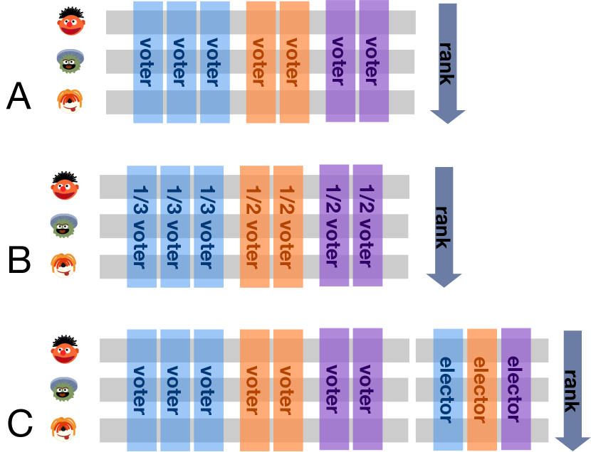
Figure 1: Three ways to run the aggregation procedures. A: Basic aggregation. B: Weighted aggregation. C: Two-step aggregation.

3 Case Studies

This section describes four case studies on three NLP and multimodal benchmarks. Our main objective here is to re-interpret the benchmarking trends under the social choice theory. We provide a brief description of the benchmarks below.

• GLUE (General Language Understanding Evaluation; Wang et al., 2018) combines nine datasets on QA, sentiment analysis, and textual entailment. GLUE also includes a linguistic diagnostic test set. $|M|$=$30$.

• SGLUE (Wang et al., 2019a) is the GLUE follow-up consisting of two diagnostic and eight more complex NLU tasks, ranging from causal reasoning to multi-hop and cloze-style QA. $|M|$=$22$.

• VALUE (Video-and-Language Understanding Evaluation; Li et al., ) covers 11 video-and-language datasets on text-to-video retrieval, video QA, and video captioning. $|M|$=$7$.

The leaderboards present the results of evaluating various neural models, such as BERT (Devlin et al., 2019), StructBERT (Wang et al., 2019b), ALBERT (Lan et al., 2019), RoBERTa (Liu et al., 2019), T5 (Raffel et al., 2020), DeBERTa (He et al., 2020), ERNIE (Zhang et al., 2019), and their ensembles and other model configurations.

3.1 Re-interpreting Benchmarks

Benchmark	$k$	$\sigma^{gm}$	$\sigma^{og}$	Copeland	Minimax	Plurality	Dowdall	Borda
GLUE	top-$1$	1.0	1.0	1.0	1.0	1.0	1.0	1.0
	top-$3$	1.0	0.67	1.0	0.67	0.67	0.67	1.0
	top-$5$	1.0	0.80	0.60	0.80	0.80	0.80	0.8
	top-$7$	1.0	0.86	0.86	0.86	0.86	0.86	1.0
	least-$5$	0.67	0.00	1.0	0.33	0.33	1.0	1.0
	least-$7$	0.86	0.71	1.0	0.14	0.14	1.0	1.0
	$\tau$	0.56	-0.08	0.23	-0.05	0.03	0.28	0.41
SGLUE	top-$1$	1.0	1.0	0.00	1.0	0.00	0.00	1.0
	top-$3$	1.0	1.0	0.67	0.67	0.67	0.67	1.0
	top-$5$	1.0	1.0	1.0	1.0	0.80	1.0	1.0
	top-$7$	1.0	0.86	0.86	0.71	0.57	0.86	0.86
	least-$5$	1.0	1.0	1.0	0.33	0.33	1.0	1.0
	least-$7$	0.86	0.86	0.86	0.14	0.14	0.86	1.0
	$\tau$	0.45	0.36	0.08	-0.5	-0.15	0.12	0.24

Table 1: Agreement rates between the top/least-$k$ rankings with $\sigma^{am}$. The Kendall Tau correlation ($\tau$) is computed on the total rankings.

Method. We begin with a case study on re-ranking systems on the publicly available leaderboards using the scoring and majority-relation based rules: Plurality, Dowdall, Borda, Copeland, and Minimax as the baselines. $\sigma^{og}$ is an aggregation metric that identifies the amount by which the system fails to get a minimum score of $\gamma=0.95$ (lower is better). The comparison is run by computing (i) the agreement rate (AR; in %), i.e. the proportion of the top/least-$k$ systems between the given procedure and $\sigma^{am}$, (ii) the Kendall Tau correlation ($\tau$) between the total rankings, (iii) the discriminative power (DP) or the number of tied alternatives. i.e. alternatives with the same score (Brandt and Seedig, 2016), and (iv) the independence of irrelevant alternatives (IIA), i.e. how often the new systems change the ranking (see Appendix A.2 for details). IIA is computed iteratively in two steps. First, we initialise a leaderboard with two random systems $m_{A}$ and $m_{B}$. Second, we add a new random system $m_{C}$ to the leaderboard and check if the rankings of $m_{A}$ and $m_{B}$ have changed. We repeat the procedure by adding up to $|M|$ systems and counting how often the new system affects the ranking. The experiment is run $50$ times to account for randomness.

Method	GLUE		SGLUE
	DP	IIA	DP	IIA
$\sigma^{am}$	1	0.0 $\pm$0.0	0	0.0 $\pm$0.0
$\sigma^{gm}$	0	0.0 $\pm$0.0	0	0.0 $\pm$0.0
$\sigma^{og}$	3	0.0 $\pm$0.0	1	0.0 $\pm$0.0
Copeland	6	2.76 $\pm$1.3	2	0.90 $\pm$0.8
Minimax	21	2.94 $\pm$1.5	17	1.14 $\pm$1.0
Plurality	25	5.26 $\pm$1.6	17	1.98 $\pm$1.4
Dowdall	0	9.10 $\pm$2.4	0	4.24 $\pm$2.1
Borda	0	7.96 $\pm$3.8	1	5.38 $\pm$1.8

Table 2: Discriminative power (DP) and independence of irrelevant alternatives (IIA) values. The lower, the better for both DP and IIA.

Results. Table 1 and Table 2 present the results except for the VALUE benchmark which is discussed in Appendix B. We find that methods tend to agree on the top systems, but Minimax and Plurality disagree on which ones are the worst. Despite high ARs on particular top/least-$k$ systems, the order of the systems on GLUE and SGLUE is different, which is indicated by the low correlation coefficients. The Pythagorean mean results are consistent with one another on the top-$7$ systems and may lead to different worst systems. $\sigma^{og}$ generally disagrees with $\sigma^{am}$ for the top and worst systems on GLUE but has higher ARs and correlation on SGLUE.

At the same time, the DP results demonstrate that Dowdall and Borda produce only one pair of alternatives with the same score, whilst Minimax and Plurality treat a significantly larger number of systems as equivalent. The reason is that the rules initially intend to define the best alternative, and they are indecisive between the alternatives when utilised to rank. The IIA experiment shows that introducing a new system influences the Dowdall and Borda rankings. However, this tendency is less common for Copeland, Minimax, and Plurality and is observed only up to $2$ times on SGLUE.

Rank	$\sigma^{am}$	$\sigma^{gm}$	$\sigma^{og}$	Copeland	Minimax	Plurality	Dowdall	Borda
1	91.18	${}_{\updownarrow 0}^{90.89}$	${}_{\updownarrow 0}^{0.074}$	${}_{\updownarrow 0}^{29.00}$	${}_{\updownarrow 0}^{0}$	${}_{\updownarrow 0}^{2.00}$	${}_{\updownarrow 0}^{4.95}$	${}_{\updownarrow 0}^{260.50}$
2	91.07	${}_{\updownarrow 0}^{90.78}$	${}_{\uparrow 4}^{0.075}$	${}_{\uparrow 1}^{25.00}$	${}_{\uparrow 1}^{-5.50}$	${}_{\uparrow 13}^{2.00}$	${}_{\uparrow 13}^{4.08}$	${}_{\updownarrow 0}^{256.00}$
3	90.88	${}_{\updownarrow 0}^{90.56}$	${}_{\downarrow 1}^{0.076}$	${}_{\downarrow 1}^{24.00}$	${}_{\uparrow 1}^{-6.00}$	${}_{\updownarrow 0}^{1.50}$	${}_{\updownarrow 0}^{3.82}$	${}_{\updownarrow 0}^{247.50}$
4	90.86	${}_{\updownarrow 0}^{90.48}$	${}_{\updownarrow 0}^{0.076}$	${}_{\uparrow 3}^{22.00}$	${}_{\downarrow 2}^{-6.50}$	${}_{\uparrow 1}^{1.00}$	${}_{\updownarrow 0}^{3.41}$	${}_{\updownarrow 0}^{241.50}$
5	90.74	${}_{\updownarrow 0}^{90.44}$	${}_{\updownarrow 0}^{0.077}$	${}_{\uparrow 10}^{22.00}$	${}_{\uparrow 2}^{-7.00}$	${}_{\downarrow 3}^{1.00}$	${}_{\downarrow 3}^{3.27}$	${}_{\uparrow 1}^{233.50}$
6	90.66	${}_{\updownarrow 0}^{90.34}$	${}_{\uparrow 1}^{0.078}$	${}_{\downarrow 2}^{22.00}$	${}_{\uparrow 9}^{-7.00}$	${}_{\updownarrow 0}^{0.50}$	${}_{\downarrow 1}^{2.57}$	${}_{\uparrow 1}^{229.50}$
7	90.48	${}_{\updownarrow 0}^{90.11}$	${}_{\uparrow 3}^{0.082}$	${}_{\downarrow 1}^{16.00}$	${}_{\downarrow 1}^{-7.00}$	${}_{\downarrow 3}^{0.00}$	${}_{\updownarrow 0}^{2.55}$	${}_{\downarrow 2}^{220.50}$

Table 3: Results of re-ranking the GLUE benchmark. Changes in the system ranks are depicted with arrows, whilst the superscripts denote scores assigned by the aggregation procedure. Notations: =Human; =ERNIE; =StructBERT+CLEVER; =DeBERTa+CLEVER;=DeBERTa/TuringNLRv4; =MacALBERT+DKM;=T5; =ALBERT+DAAF+NAS;=Funnel. The superscript values stand for the voting rules’ scores, whilst the subscript values indicate changes in the ranking positions. $\uparrow x$ means up $x$ positions, $\downarrow x$ means down $x$ positions, $\updownarrow$ means no changes.

Overall, we observe that the GLUE and SGLUE benchmark rankings depend on the aggregation procedure. The human baseline (Human) rank has risen by up to $13$ positions on GLUE (see Table 3). The Copeland method takes Human, DeBERTa+CLEVER, and T5 equal, meaning that the difference between the number of candidates they dominate and are dominated by is the same. The Minimax ranking suggests that Human, T5, and the ALBERT+DAAF+NAS ensemble are equivalent, meaning that minimal maximum defeats against other models are the same. In their turn, the Plurality and Dowdall procedures rank Human as the second-best solution, since Human receives the best performance in several tasks, such as RTE (Wang et al., 2018) and MNLI (Williams et al., 2018). The tendency is also observed on the SGLUE benchmark (see Table 9 in Appendix B), with the exception that Human is selected as the winner by the Copeland, Plurality, and Dowdall procedures and is equal to the ERNIE system according to Minimax. The results for Borda are similar to $\sigma^{am}$ and $\sigma^{gm}$ on the top-$4$ and top-$6$ ranks on GLUE and SGLUE, respectively.

Selecting the winner. Another application of the voting rules includes selecting the winner from the set of alternatives. Here, we also utilise the Threshold, Baldwin, and Condorcet rules. Note that we run the VALUE experiment over missing and non-missing scores since the Human results are presented for only $6$ out of $11$ tasks.

Results. Table 4 presents the results of selecting the winner for each benchmark. ✗ denotes that (i) the given method does not support missing values, or (ii) there is no Condorcet winner (CW). We observe that different SoTAs are selected by $2$/$7$/$3$ (on GLUE/SGLUE/VALUE) procedures as opposed to $\sigma^{am}$, $\sigma^{gm}$, and $\sigma^{og}$. The Threshold rule selects T5+UDG and StructBERT+CLEVER as winners because their performance is the worst the least amount of times. The Baldwin rule agrees with the Plurality and Minimax results. When considering VALUE missing scores, we find that Human is declared SoTA by the Copeland, Minimax, and Condorcet procedures. It means that Human beats any other model in pairwise comparison and is declared the CW, whilst significantly outperforming the systems on specific tasks.

Method	GLUE	SGLUE	VALUE
$\sigma^{am}$			✗/
$\sigma^{gm}$			✗/
$\sigma^{og}$			✗/
Copeland			/
Minimax			/
Plurality			✗/
Dowdall			✗/
Borda			✗/
Threshold			✗/
Baldwin			✗/
Condorcet		✗	/

Table 4: The winner selection results. Notations:

=StructBERT+CLEVER;

=Human;

=craig.starr;

=ERNIE;

=T5+UDG.

Case study discussion. Benchmarks can suffer from saturation, which is characterised by surpassing estimates of the human performance followed by stagnation in SoTA improvements (Ott et al., 2022). The NLP community has discussed saturation of the GLUE benchmark over time (Kiela et al., 2021; Ruder, 2021) and minor performance gains of the upcoming top-leading systems on SGLUE (Rogers, 2019). However, the discussion relies on the mean aggregation. Let us take a step away from the utilitarian approach. We observe that Human may still take leading positions, and system ranking varies on these benchmarks under the social choice theory principles. VALUE demonstrates more stable results in terms of the AR and the system order, which we attribute to its novelty and minor performance differences between the systems. Overall, our rules provide interpretable results and cope with the missing leaderboard values in contrast to the utilitarian methods.

3.2 The Condorcet Winner

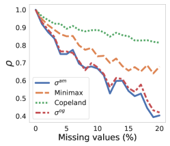
(a) GLUE

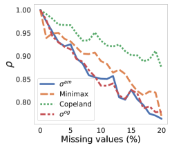
(b) SGLUE

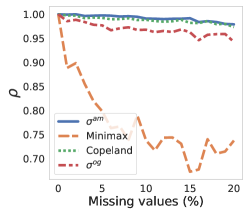
(c) VALUE

Figure 2: Spearman correlation ($\rho$) between top-$7$ model rankings with/without omitted leaderboard values for $\sigma^{am}$, $\sigma^{og}$, Minimax, and Copeland rankings. The results are averaged over $100$ runs.

One of the most natural ways to choose the best system given a set of weights defined by the user is the Condorcet method, which declares a system the winner if it dominates all other alternatives in pairwise comparison (Black et al., 1958). The Condorcet method is hard to destabilise (Edelman, 2015) and easy to interpret in practice, indicating that the CW best matches the preferences. Given the weights vector, finding the CW, if it exists, is trivial. We can also find the weights that make a given alternative the CW or determine that no weights with that property exist.

Method. Let us define an operator $R(m_{1},m_{2},i)$:

A system $m$ is declared a CW if the following property is satisfied:

Let $G_{m}\in\{-1,0,1\}^{|M|-1\times|T|}$ be a matrix such that $G_{ij}=R(m,m_{i}^{\prime},j)$, where $\{m^{\prime}_{1},..,m^{\prime}_{|M|-1}\}=M\setminus\{m\}$.

Equation 2 can be re-written as: $G_{m}\cdot w\succcurlyeq 0$, which results in defining a space $W^{*}$ in $\mathbb{R}^{|T|}$, whose each point is a weight vector making $m$ a CW. Any linear algorithm can be applied to find a point in $W^{*}$ or determine that $W^{*}$ is empty. Furthermore, any other linear conditions can be added, such as upper/lower bounds of the $w$ components and a linear function that needs to be optimised, e.g. $w_{i}\longrightarrow\min$. Let us call a system for which there exists a vector of weights making it a CW prospective. By definition, the system is prospective if $W^{*}$ is not empty.

Example. Let us illustrate the method on the SGLUE benchmark (see Table 4). There is no CW if the task weights are assigned uniformly. Nevertheless, T5 may become the CW when the BoolQ accuracy (Clark et al., 2019) and MultiRC exact match scores (Khashabi et al., 2018) have equal weights of $0.5$, and the other criteria weights are zeroed. In this scenario, T5 has been found to be a prospective system on SGLUE, whiste RoBERTa is declared non-prospective.

Results. There are $9$/$88$, $10$/$12$, and $3$/$3$ prospective/non-prospective systems on GLUE, SGLUE, and VALUE, respectively. The results indicate that it is possible to find specific evaluation scenarios in which a given system is the best. In contrast, the non-prospective system always has an alternative that performs neither worse nor better.

Case study discussion. The CW criterion presents another perspective of selecting the best systems. Notably, the existence of the CW weights assumes that practitioners can simulate a set of real-world scenarios where the system is the best across the given axes. Specifying if the system can be the CW on the leaderboard would help diagnosing the systems without additional heavy experiments. The developers also can document this information on model sharing platforms, e.g. HuggingFace (Wolf et al., 2020).

3.3 Robustness to Missing Scores

This case study considers a more detailed analysis of the majority-relation based voting rules that can be efficiently utilised for ranking systems and selecting the winner over missing scores. Here, we evaluate the robustness of the rules to omitted performance scores and analyse how the rankings change under such perturbation.

Method. Copeland and Minimax take as input the majority graph in which each vertex corresponds to a candidate and an edge from the candidate $m_{1}$ to $m_{2}$ exists iff $m_{1}\mu m_{2}$, i.e. $m_{1}$ is ranked higher than $m_{2}$ by more criteria. Let us say there are $T$ criteria $t\in\{t_{1},\ldots,t_{T}\}$ and $w\in\{w_{1},\ldots,w_{n}\}$ are the weights assigned to them.

When evaluating $R(m_{1},m_{2},i)$, this approach can handle missing values, ignoring the pairs where either of the scores is missing. We can apply the majority-relation based rules using relation $\mu$ to rank alternatives with missing scores without losing any information whilst accounting for the available criteria.

We analyse the robustness of the Copeland and Minimax rules as follows. First, we compute the rankings using both methods on each benchmark without omitting scores and use them as references. Next, we randomly replace $N$ scores with empty values and find top-$7$ systems over the corrupted leaderboards. We calculate the Spearman correlation ($\rho$) between the final rankings and the references. Note that we use the median values when omitting scores for $\sigma^{am}$ and $\sigma^{og}$ as the baselines.

Results.  Figure 2 shows that $\sigma^{am}$ and $\sigma^{og}$ display lower stability and Copeland performs the best on GLUE and SGLUE. However, we observe that Minimax is the least stable on VALUE, whilst Copeland, $\sigma^{am}$, and $\sigma^{og}$ perform on par.

Case study discussion. We attribute the low stability of Minimax on VALUE to its limitations. Recall that there are minor differences between the systems on VALUE, which cause Minimax to score them very similar (see Table 10 in Appendix B). In this case any missing value can influence the rankings, which results in the low $\rho$ coefficients.

3.4 Ranking Based on User Preferences

Rank	$\sigma^{am}_{\text{{Performance}}}$	Borda	Weighted Borda	Weighted 2-step Borda	Borda Performance	Borda Efficiency	Borda Fairness
1	82.73	${}_{\uparrow 4}^{267.0}$	${}_{\uparrow 5}^{10.75}$	${}_{\uparrow 2}^{4.30}$	${}_{\updownarrow 0}^{56.5}$	${}_{\uparrow 4}^{223.0}$	${}_{\uparrow 2}^{19.0}$
2	82.52	${}_{\uparrow 4}^{245.0}$	${}_{\uparrow 1}^{9.83}$	${}_{\uparrow 2}^{3.60}$	${}_{\updownarrow 0}^{49.0}$	${}_{\uparrow 4}^{216.0}$	${}_{\uparrow 4}^{18.0}$
3	80.94	${}_{\uparrow 1}^{166.0}$	${}_{\uparrow 1}^{8.96}$	${}_{\uparrow 3}^{3.40}$	${}_{\updownarrow 0}^{32.5}$	${}_{\uparrow 1}^{120.0}$	${}_{\uparrow 1}^{14.0}$
4	79.20	${}_{\downarrow 1}^{154.0}$	${}_{\uparrow 1}^{8.63}$	${}_{\downarrow 3}^{3.00}$	${}_{\updownarrow 0}^{32.0}$	${}_{\downarrow 1}^{103.0}$	${}_{\downarrow 3}^{11.00}$
5	78.56	${}_{\downarrow 3}^{144.0}$	${}_{\downarrow 4}^{7.17}$	${}_{\updownarrow 0}^{2.90}$	${}_{\updownarrow 0}^{17.0}$	${}_{\downarrow 3}^{91.0}$	${}_{\uparrow 1}^{11.0}$
6	77.89	${}_{\uparrow 1}^{10.0}$	${}_{\downarrow 4}^{7.04}$	${}_{\downarrow 3}^{2.60}$	${}_{\updownarrow 0}^{11.0}$	${}_{\uparrow 1}^{84.0}$	${}_{\uparrow 1}^{7.00}$
7	75.95	${}_{\downarrow 6}^{70.50}$	${}_{\updownarrow 0}^{5.47}$	${}_{\updownarrow 0}^{0.90}$	${}_{\updownarrow 0}^{8.0}$	${}_{\downarrow 6}^{3.00}$	${}_{\downarrow 5}^{4.00}$

Table 5: Results of re-ranking the GLUE benchmark using the Borda rule in the simulated user-oriented scenario. Notations: = ALBERT; =BERT; =DistilBERT; =RoBERTa; =DistilRoBERTa; =DeBERTa; =GPT2.

This case study aims at system ranking based on the user utility. We rank systems in a simulated scenario that considers preferences on performance, computational efficiency, and fairness.

Method. We use the HuggingFace library to fine-tune and evaluate systems on GLUE. Each system is initialised with a fixed set of five random seeds and fine-tuned for five epochs with default hyper-parameters and a batch size of $16$. The development set performance is averaged across all runs. We consider the following systems: BERT-base, RoBERTa-base, ALBERT-base, DeBERTa-base, DistilBERT-base (Sanh et al., 2019), DistilRoBERTa-base (Sanh et al., 2019), and GPT2-medium (Radford et al., 2019). The experiments are run on a single GPU unit, NVIDIA A100 80 GB SXM (NVLink), $4$-CPU cores, AMD EPYC 7702 2-3.35 GHz, and 1 TB RAM.

The efficiency is computed during fine-tuning via the Impact tracker toolkit (Henderson et al., 2020): the total power, run time in hours, GPU usage in hours, and estimated carbon footprint. To maximise these, we inverse the computational efficiency features through multiplying them by $-1$.

To measure fairness, we choose three social bias evaluation datasets: CrowS-Pairs (Nangia et al., 2020), StereoSet (Nadeem et al., 2021), and Winobias (Zhao et al., 2018). In these datasets, one sentence is always more stereotyping than the other. Following Nangia et al. (2020), we use MLM scoring (Salazar et al., 2020) to score the pairs. The final metrics account for cases (%) in which a less stereotyping sentence is the most probable.

For the sake of space, we present the results on the Borda procedure in the basic, weighted, and two-step aggregation settings (§2.4). We assign the weights vector as $(0.4,0.3,0.3)$ to performance, efficiency, and fairness. The weights are introduced to increase the impact of performance. We use $\sigma^{am}$ as the baseline and interim rankings by each criterion individually as references.

Results. Table 5 shows that DeBERTa is the winner according to $\sigma^{am}$ and Borda. However, it requires more computational resources than the other systems and is mediocre in detecting social biases. As a result, it is not the best system in any user-oriented ranking. In this scenario, Borda tends to favour the distilled systems (DistilRoBERTa and DistilBERT) due to their computational efficiency, which has the highest impact on the ranking with four criteria assigned per task. The weighted Borda ranks DistilBERT, ALBERT, and BERT as the top-$3$ systems. In its turn, the weighted $2$-step Borda prefers ALBERT first, followed by BERT and DistilBERT. ALBERT is selected as the winner by the fairness ranking only and occupies the middle positions in the two other rankings. RoBERTa drops down drastically from the second rank ($\sigma^{am}$), whilst GPT2 remains in the least-$3$ systems.

Case study discussion. Overall, our setup follows Dynascore (Ma et al., 2021), where the microeconomic concept of MRS is used to compare performance, efficiency, and fairness metrics, followed by the weighted average score as the final ranking. Unlike the Dynascore results, we find that the average performance ranking is not preserved when using our voting rules. The most notable difference is with DeBERTa and RoBERTa systems, which may become penalised for low efficiency in our case. The reason is that in Dynascore, the weight of $0.5$ is assigned to performance which blocks substantial changes in re-ranking.

4 Recommendations for Rules Choice

The information about the voting rules’ properties can be used to choose the most suitable one to the user’s preferences Felsenthal and Machover (2012). We also provide the following recommendations.

• The Plurality rule is a good choice if the user wants only the best systems in each criterion.

• If all ranking positions matter, use the Borda or Dowdall rules. Note that Dowdall assigns higher weights to the top positions.

• The Threshold rule is helpful in cases when the user wants to minimise the number of the low-performance criteria: the rule assigns the highest rank to the system that is considered the worst in the least amount of criteria.

• If the goal is to select the system that beats all the others in pairwise comparison, use the Baldwin, Condorcet, Copeland, or Minimax rules. These rules are Condorcet consistent; i.e. choose the CW if it exists. The main difference is how the rules behave when there is no CW. In particular, Baldwin selects the system that is left after elimination according to the Borda scores. Copeland chooses the system that dominates the others in more cases and is dominated by the least. In turn, Minimax selects the system with minimum defeat in pairwise comparison.

• The outcomes may contain equivalent alternatives (§3.1). Depending on the scenario, the user can select the rule that produces ties with a lower probability or Dowdall and Borda if their properties meet the preferences.

5 Conclusion and Future Work

This paper introduces novel aggregation procedures to rank and select the best-performing systems under the social choice theory principles. Our approach provides an alternative perspective of system evaluation in benchmarking and overcomes the standard mean aggregation limitations.

Our case studies show that Vote’n’Rank provides interpretable decisions on the best and worst systems whilst accounting for missing performance scores and potential user preferences. The framework allows for finding scenarios in which a given system dominates the others. At the same time, the rule choice may depend on the particular research and development purpose. We provide recommendations based on the rules’ properties and scenarios of the intended framework’s application.

The application scope of Vote’n’Rank is not limited and may be easily extended to other applied ML areas. The current mainstay of multilingual and multimodal benchmarking fails to provide a nuanced comparison of systems across languages and tasks. In our future work we hope to explore applications of the social choice theory in this direction through a consideration of user studies and an extended set of voting rules and linguistic criteria.

6 Limitations

Robustness. In the robustness experiments, the Copeland and Minimax rules are less sensitive to performance score drops than $\sigma^{am}$ and $\sigma^{og}$. However, in certain circumstances Minimax may display low resistance to such corruption due to its nature, which is analysed in §3.3. Other robustness evaluation settings can be considered, such as sensitivity to removing and adding new tasks (Procaccia et al., 2007; Colombo et al., ), which are out of scope of this work.

Ambiguity. Almost all rules in our study allow ties or the recognition of systems as equivalent. This may result in non-resoluteness: the selection of multiple winning systems or the presence of many equivalencies in ranking. However, we empirically observe no or a few ties using the Dowdall, Borda, and Copeland rules, whilst Minimax and Plurality treat a significant number of systems as equivalent due to their properties (§3.1). Vote’n’Rank does not currently support any additional tie-breaking rules to be applied in this case. The only exception here is the Threshold rule that gives only one winner in almost all cases due to the built-in tie-breaking procedure.

Independence of irrelevant alternatives. The violation of the IIA axiom in applications is a well-known fundamental aspect in the social choice theory, and the voting rules can violate the IIA with different probabilities Dougherty and Heckelman (2020). IIA violation may imply undesirable behavior: submitting a new system to the leaderboard affects the relative ranking of the other systems. However, we empirically show that Copeland and Minimax are less likely to violate IIA than Plurality and Borda rules (§3.1). The IIA assumption may be unrealistic in practice as it takes no account of perfect or near-perfect substitutes Suppes (1965).

Lack of ground truth. Comparison of the aggregation procedures is hindered by the absence of the correct ranking, especially when votes are noisy and incomplete. There is no universal answer to the question of how the systems on the multi-task benchmarks should be preferred. However, we hope to contribute from a practical standpoint, offering an alternative approach to the mean aggregation procedure.

7 Ethical Considerations

Stereotypes and discrimination in LMs’ pre-training data can lead to representation biases against race, religion, and social minorities. Our framework allows ranking systems to account for sensitive attributes (Celis et al., 2018), e.g. gender and nationality, or to find the trade-off between multiple criteria, e.g. performance and fairness (Baldini et al., 2022). The rank aggregation rules have been widely adopted to information retrieval and recommendation systems (Dwork et al., 2001; Masthoff, 2011). We assume that translation of the social choice theory into the system evaluation problems may improve the user experience by selecting systems that best satisfy evaluative criteria and individual or group preferences in downstream applications.

Appendix A Aggregation Procedures

A.1 Examples

Rank	Task 1	Task 2	Task 3	Task 4	Task 5
1	$m_{A}$	$m_{A}$	$m_{B}$	$m_{C}$	$m_{D}$
2	$m_{B}$	$m_{C}$	$m_{D}$	$m_{B}$	$m_{B}$
3	$m_{C}$	$m_{D}$	$m_{C}$	$m_{D}$	$m_{C}$
4	$m_{D}$	$m_{B}$	$m_{A}$	$m_{A}$	$m_{A}$

Table 6: A toy leaderboard for illustration purposes.

Rank	Task 1	Task 2	Task 3	Task 4	Task 5
1	$m_{B}$	$m_{C}$	$m_{B}$	$m_{C}$	$m_{D}$
2	$m_{C}$	$m_{D}$	$m_{D}$	$m_{B}$	$m_{B}$
3	$m_{D}$	$m_{B}$	$m_{C}$	$m_{D}$	$m_{C}$

Table 7: The leaderboard based on Table 6 used for describing the Baldwin rule.

This appendix provides illustrative examples on how our voting rules work. Here, suppose we have a toy leaderboard with five tasks and four systems as shown in Table 6. The systems are ranked within each task by their performance score. We now compute the rankings using each voting rule.

Scoring rules.

• Plurality rule assigns the score of $2$ to $m_{A}$ and scores of $1$ to $m_{B}$, $m_{C}$, and $m_{D}$.

• According to the Borda rule, the systems that take the first position get $3$ points for each task, $2$ points are awarded for the second position, etc. As a result, the systems receive the following Borda scores: $m_{A}=6$, $m_{B}=9$, $m_{C}=8$, and $m_{D}=7$. The system $m_{B}$ has the highest score and is chosen as the best one.

• For the Dowdall rule scoring vector, we get the following scores: $S_{m_{A}}=2.75$, $S_{m_{B}}=2.75$, $S_{m_{C}}=2.5$, and $S_{m_{D}}=1.75+2/3$. There is a tie between the systems $m_{A}$ and $m_{B}$, and both of them are considered the best models.

Iterative scoring rules.

• For the Threshold rule scoring vector (1,1,1,0), we get the following scores: $S_{m_{A}}=2$, $S_{m_{B}}=4$, $S_{m_{C}}=5$, and $S_{m_{D}}=4$. The system $m_{C}$ is the winner. If there is a tie, the scoring vector (1,1,0,0) is further applied for only tied systems.

• The Baldwin rule: first, we calculate the Borda scores as mentioned above. Second, we eliminate the system $m_{A}$ since it has the lowest score (see Table 7). Next, we re-calculate the Borda scores for a new scoring vector (2,1,0) and get the following results: $S_{m_{B}}=6$, $S_{m_{C}}=5$, and $S_{m_{D}}=4$. At this step, the system $m_{D}$ is eliminated. Finally, we re-calculate the results for the scoring vector (1,0). The results are $S_{m_{B}}=3$ and $S_{m_{C}}=2$, and the system $m_{B}$ is declared the winner.

Majority-relation based rules.

The majority relation in this example is illustrated in Figure 3.

• The system $m_{B}$ is the Condorcet winner as it beats each of the alternatives. Note that since all majority-relation based rules (Copeland and Minimax) are Condorcet consistent, they declare the system $m_{B}$ the winner as well. Let us illustrate it in more detail.

• The Copeland rule scores are $u(m_{A})=-3$, $u(m_{B})=3$, $u(m_{C})=1$, $u(m_{D})=-1$. The system $m_{B}$ is the winner as it has the highest $u(x)$.

• The Minimax rule scores are $rank(m_{A})=-3$, $rank(m_{B})=0$, $rank(m_{C})=-3$, $rank(m_{D})=-3$. Here, the system $m_{B}$ has the highest rank.

Figure 3: A toy graph example of the majority relation $\mu$ based on Table 6.

A.2 Properties

We consider the following properties to describe our voting rules and summarise them in Table 8.

	Plurality	Borda	Dowdall	Threshold	Baldwin	Copeland	Minmax
Transitivity	✓	✓	✓	✓	✓	✓	✓
Anonymity	✓	✓	✓	✓	✓	✓	✓
Unanimity	✓∗	✓	✓	✓	✓	✓	✓
IIA	✗	✗	✗	✗	✗	✗	✗
Monotonicity	✓	✓	✓	✓	✗	✓	✓
Majority	✓	✗	✓	✗	✓	✓	✓
CW	✗	✗	✗	✗	✓	✓	✓
Condorcet loser	✗	✓	✗	✗	✓	✓	✗
Sum	5	5	5	4	6	7	6

Table 8: Rules and their properties. ^∗The non-winning Pareto-dominated systems can be tied.

• Transitivity. There are no cycles in the final ranking. An example of the cycle is a situation, where $m_{A}$ is better than $m_{B}$, $m_{B}$ is better than $m_{C}$, and $m_{C}$ is better than $m_{A}$.

• Unanimity (Pareto efficacy). If the system $m_{A}$ is ranked higher than $m_{B}$ according to all criteria, then $m_{A}$ should be ranked higher.

• Non-dictatorship (Anonymity). There is no single criterion that defines the final ranking.

• Independence of irrelevant alternatives (IIA). For any two systems, the information about other systems should not influence their ranking.

• Monotonicity. If the system $m_{A}$ is the winner and it started to rank higher according to one of the criteria, then it should still be the winner.

• Majority criterion. If the system $m_{A}$ is considered the best by more than 50% criteria, then it should be the winner.

• Condorcet winner criterion. This criterion is a stronger version of the Majority criterion. If the system $m_{A}$ is the Condorcet winner (CW), it should be the winner according to the rule.

• Condorcet loser criterion. If the system $m_{A}$ is the Condorcet loser ($a\mu M^{L}$ for any $a\in A$), it should never be the winner according to the rule.

Recall that the Condorcet rule by definition complies with the Condorcet winner and loser criteria. The other properties can not be checked in application to benchmarking since the rule is defined on a restricted domain: it does not provide the results on any possible combination of rankings.

There is no single best voting rule since none of them satisfies properties of the Arrow’s impossibility theorem Arrow (2012); Geanakoplos (2005): transitivity, unanimity, non-dictatorship, and independence of irrelevant alternatives (IIA).

Appendix B Case Studies

We do not report the agreement rate, the Kendall Tau ($\tau$) correlation, and the IIA results for VALUE since we are given only up to $7$ evaluated alternatives: craig.starr (Shin et al., 2021), DuKG (Li et al., 2021), Human, and four HERO-based configurations (Li et al., 2020). The HERO-based baselines are trained in the following settings: single-task training (ST), multi-task training (MT) by tasks or domains, all-task training (AT) and AT first then ST (AT -> ST). We refer to the configurations as follows:

• HERO₁: AT->ST, PT+FT;

• HERO₂: AT->ST, FT-only;

• HERO₃: ST, PT+FT;

• HERO₄: ST, FT-only.

The VALUE results. Table 10 and Table 11 show the VALUE re-ranking results over missing/non-missing scores. ✗ means that the given aggregation method does not operate over missing values. In the first case, we observe that the Copeland and Minimax rules generally agree on the final outcomes except for the fifth and sixth positions. The rules select Human as the winner. At the same time DuKG and HERO₁ have the same Minimax values, and the Minimax values of the least-$3$ systems are also equal. In the second case, we omit Human due to missing scores on $6$ out of $11$ tasks for comparable interpretation. However, there are $3$ tied alternatives in the Minimax and Dowdall outcomes. Interestingly, all methods are consistent in conclusions on the top-$3$ systems, with the Minimax treating DuKG and HERO₁ as equal alternatives. The $\sigma^{og}$, Minimax, Plurality, Dowdall, and Borda rules make equal decisions on the final outcomes.

Rank	$\sigma^{am}$	$\sigma^{gm}$	$\sigma^{og}$	Copeland	Minimax	Plurality	Dowdall	Borda
1	90.62	${}_{\updownarrow 0}^{90.04}$	${}_{\updownarrow 0}^{0.066}$	${}_{\uparrow 3}^{20.00}$	${}_{\updownarrow 0}^{0}$	${}_{\uparrow 3}^{4.00}$	${}_{\uparrow 3}^{4.98}$	${}_{\updownarrow 0}^{155.00}$
2	90.39	${}_{\updownarrow 0}^{89.84}$	${}_{\updownarrow 0}^{0.068}$	${}_{\downarrow 1}^{19.00}$	${}_{\uparrow 2}^{0}$	${}_{\downarrow 1}^{2.50}$	${}_{\downarrow 1}^{4.25}$	${}_{\updownarrow 0}^{154.50}$
3	90.29	${}_{\updownarrow 0}^{89.75}$	${}_{\updownarrow 0}^{0.068}$	${}_{\downarrow 1}^{18.00}$	${}_{\downarrow 1}^{-4.50}$	${}_{\downarrow 1}^{1.00}$	${}_{\downarrow 1}^{3.62}$	${}_{\updownarrow 0}^{153.00}$
4	89.79	${}_{\updownarrow 0}^{88.80}$	${}_{\uparrow 1}^{0.073}$	${}_{\downarrow 1}^{15.00}$	${}_{\downarrow 1}^{-5.00}$	${}_{\downarrow 1}^{0.50}$	${}_{\downarrow 1}^{3.29}$	${}_{\updownarrow 0}^{145.50}$
5	89.25	${}_{\updownarrow 0}^{88.75}$	${}_{\downarrow 1}^{0.074}$	${}_{\updownarrow 0}^{13.00}$	${}_{\updownarrow 0}^{-7.50}$	${}_{\uparrow 9}^{0.00}$	${}_{\updownarrow 0}^{2.11}$	${}_{\updownarrow 0}^{141.50}$
6	86.65	${}_{\updownarrow 0}^{85.93}$	${}_{\uparrow 1}^{0.089}$	${}_{\updownarrow 0}^{11.00}$	${}_{\uparrow 8}^{-8.00}$	${}_{\uparrow 12}^{0.00}$	${}_{\updownarrow 0}^{1.16}$	${}_{\updownarrow 0}^{116.50}$
7	86.09	${}_{\updownarrow 0}^{85.38}$	${}_{\uparrow 5}^{0.10}$	${}_{\uparrow 1}^{9.00}$	${}_{\uparrow 11}^{-8.00}$	${}_{\uparrow 12}^{0.00}$	${}_{\uparrow 1}^{1.06}$	${}_{\uparrow 1}^{108.00}$

Table 9: Results of re-ranking the SGLUE benchmark. The model rank changes are depicted with arrows, whilst the superscripts denote scores assigned by the voting method. Notations: =Human; =ERNIE; =DeBERTa/TuringNLRv4; =NEZHA-Plus; =T5+UDG; =BERT++; =PAI Albert; =RoBERTa-iCETS; =GPT-3 few-shot; =iPET (ALBERT) few-shot; =T5;=AILabs Team.

Rank	$\sigma^{am}$	$\sigma^{gm}$	$\sigma^{og}$	Copeland	Minimax	Plurality	Dowdall	Borda
1	✗	✗	✗	${}_{\updownarrow 0}^{6.00}$	${}_{\updownarrow 0}^{0}$	✗	✗	✗
2	✗	✗	✗	${}_{\updownarrow 0}^{4.00}$	${}_{\updownarrow 0}^{-6.00}$	✗	✗	✗
3	✗	✗	✗	${}_{\updownarrow 0}^{2.00}$	${}_{\updownarrow 0}^{-10.00}$	✗	✗	✗
4	✗	✗	✗	${}_{\updownarrow 0}^{0.00}$	${}_{\updownarrow 0}^{-10.00}$	✗	✗	✗
5	✗	✗	✗	${}_{\updownarrow 0}^{-2.00}$	${}_{\updownarrow 0}^{-11.00}$	✗	✗	✗
6	✗	✗	✗	${}_{\updownarrow 0}^{-4.00}$	${}_{\updownarrow 0}^{-11.00}$	✗	✗	✗
7	✗	✗	✗	${}_{\updownarrow 0}^{-6.00}$	${}_{\updownarrow 0}^{-11.00}$	✗	✗	✗

Table 10: Results of re-ranking the VALUE benchmark over missing scores. Changes in the system ranks are depicted with arrows, whilst the superscripts denote scores assigned by the aggregation procedure. Notations: =Human; =craig.starr; =DuKG; =HERO₁; =HERO₂; =HERO₃; =HERO₄.

Rank	$\sigma^{am}$	$\sigma^{gm}$	$\sigma^{og}$	Copeland	Minimax	Plurality	Dowdall	Borda
1	62.87	${}_{\updownarrow 0}^{49.96}$	${}_{\updownarrow 0}^{0.365}$	${}_{\updownarrow 0}^{5.00}$	${}_{\updownarrow 0}^{0}$	${}_{\updownarrow 0}^{9.00}$	${}_{\updownarrow 0}^{10.00}$	${}_{\updownarrow 0}^{53.00}$
2	60.00	${}_{\updownarrow 0}^{46.30}$	${}_{\updownarrow 0}^{0.381}$	${}_{\updownarrow 0}^{3.00}$	${}_{\updownarrow 0}^{-10.00}$	${}_{\updownarrow 0}^{1.00}$	${}_{\updownarrow 0}^{5.17}$	${}_{\updownarrow 0}^{39.00}$
3	57.58	${}_{\updownarrow 0}^{44.12}$	${}_{\updownarrow 0}^{0.399}$	${}_{\updownarrow 0}^{1.00}$	${}_{\updownarrow 0}^{-10.00}$	${}_{\updownarrow 0}^{1.00}$	${}_{\updownarrow 0}^{4.08}$	${}_{\updownarrow 0}^{30.00}$
4	56.96	${}_{\updownarrow 0}^{43.22}$	${}_{\uparrow 1}^{0.403}$	${}_{\updownarrow 0}^{-1.00}$	${}_{\uparrow 1}^{-11.00}$	${}_{\uparrow 1}^{0.00}$	${}_{\uparrow 1}^{2.87}$	${}_{\uparrow 1}^{20.00}$
5	56.07	${}_{\updownarrow 0}^{42.81}$	${}_{\downarrow 1}^{0.404}$	${}_{\updownarrow 0}^{-3.00}$	${}_{\downarrow 1}^{-11.00}$	${}_{\downarrow 1}^{0.00}$	${}_{\downarrow 1}^{2.82}$	${}_{\downarrow 1}^{18.00}$
6	52.59	${}_{\updownarrow 0}^{37.56}$	${}_{\updownarrow 0}^{0.438}$	${}_{\updownarrow 0}^{-5.00}$	${}_{\updownarrow 0}^{-11.00}$	${}_{\updownarrow 0}^{0.00}$	${}_{\updownarrow 0}^{2.02}$	${}_{\updownarrow 0}^{5.00}$

Table 11: Results of re-ranking the VALUE benchmark over non-missing scores. The Human results are discarded due to missing scores. Changes in the system ranks are depicted with arrows, whilst the superscripts denote scores assigned by the aggregation procedure. Notations: =craig.starr; =DuKG; =HERO₁; =HERO₂; =HERO₃; =HERO₄.

References

- Agarwal et al. (2021) Rishabh Agarwal, Max Schwarzer, Pablo Samuel Castro, Aaron C Courville, and Marc Bellemare. 2021. Deep Reinforcement Learning at the Edge of the Statistical Precipice. Advances in Neural Information Processing Systems, 34.
- Aizerman and Aleskerov (1995) Mark Aizerman and Fuad Aleskerov. 1995. Theory of Choice, volume 38. North Holland.
- Aleskerov et al. (2010) Fuad Aleskerov, Vyacheslav V Chistyakov, and Valery Kalyagin. 2010. The threshold aggregation. Economics Letters, 107(2):261–262.
- Arrow (2012) Kenneth J Arrow. 2012. Social choice and individual values. In Social Choice and Individual Values. Yale university press.
- Baldini et al. (2022) Ioana Baldini, Dennis Wei, Karthikeyan Natesan Ramamurthy, Moninder Singh, and Mikhail Yurochkin. 2022. Your fairness may vary: Pretrained language model fairness in toxic text classification. In Findings of the Association for Computational Linguistics: ACL 2022, pages 2245–2262, Dublin, Ireland. Association for Computational Linguistics.
- Bartholdi et al. (1989) John Bartholdi, Craig A Tovey, and Michael A Trick. 1989. Voting schemes for which it can be difficult to tell who won the election. Social Choice and welfare, 6(2):157–165.
- Belz et al. (2021) Anya Belz, Shubham Agarwal, Anastasia Shimorina, and Ehud Reiter. 2021. A systematic review of reproducibility research in natural language processing. In Proceedings of the 16th Conference of the European Chapter of the Association for Computational Linguistics: Main Volume, pages 381–393, Online. Association for Computational Linguistics.
- Benavoli et al. (2016) Alessio Benavoli, Giorgio Corani, and Francesca Mangili. 2016. Should We Really Use Post-Hoc Tests Based on Mean-Ranks? Journal of Machine Learning Research, 17(5):1–10.
- Bender et al. (2021) Emily M Bender, Timnit Gebru, Angelina McMillan-Major, and Shmargaret Shmitchell. 2021. On the Dangers of Stochastic Parrots: Can Language Models Be Too Big? In Proceedings of the 2021 ACM Conference on Fairness, Accountability, and Transparency, pages 610–623.
- Black et al. (1958) Duncan Black et al. 1958. The theory of committees and elections.
- Bowman and Dahl (2021) Samuel R. Bowman and George Dahl. 2021. What will it take to fix benchmarking in natural language understanding? In Proceedings of the 2021 Conference of the North American Chapter of the Association for Computational Linguistics: Human Language Technologies, pages 4843–4855, Online. Association for Computational Linguistics.
- Brandt and Seedig (2016) Felix Brandt and Hans Georg Seedig. 2016. On the Discriminative Power of Tournament Solutions. In Operations Research Proceedings 2014, pages 53–58. Springer.
- Celis et al. (2018) L Elisa Celis, Damian Straszak, and Nisheeth K Vishnoi. 2018. Ranking with Fairness Constraints. In 45th International Colloquium on Automata, Languages, and Programming (ICALP 2018). Schloss Dagstuhl-Leibniz-Zentrum fuer Informatik.
- Choudhury and Deshpande (2021) Monojit Choudhury and Amit Deshpande. 2021. How Linguistically Fair are Multilingual Pre-trained Language Models. In Proceedings of the AAAI Conference on Artificial Intelligence, volume 35, pages 12710–12718.
- Clark et al. (2019) Christopher Clark, Kenton Lee, Ming-Wei Chang, Tom Kwiatkowski, Michael Collins, and Kristina Toutanova. 2019. BoolQ: Exploring the surprising difficulty of natural yes/no questions. In Proceedings of the 2019 Conference of the North American Chapter of the Association for Computational Linguistics: Human Language Technologies, Volume 1 (Long and Short Papers), pages 2924–2936, Minneapolis, Minnesota. Association for Computational Linguistics.
- (16) Pierre Colombo, Nathan Noiry, Ekhine Irurozki, and Stephan CLEMENCON. What are the Best Systems? New Perspectives on NLP Benchmarking. In Advances in Neural Information Processing Systems.
- Colombo et al. (2022) Pierre Jean A Colombo, Chloé Clavel, and Pablo Piantanida. 2022. InfoLM: A New Metric to Evaluate Summarization & Data2Text Generation. In Proceedings of the AAAI Conference on Artificial Intelligence, volume 36, pages 10554–10562.
- De Almeida et al. (2019) Adiel Teixeira De Almeida, Danielle Costa Morais, and Hannu Nurmi. 2019. Systems, procedures and voting rules in context: A primer for voting rule selection, volume 9. Springer.
- Dehghani et al. (2021) Mostafa Dehghani, Yi Tay, Alexey A Gritsenko, Zhe Zhao, Neil Houlsby, Fernando Diaz, Donald Metzler, and Oriol Vinyals. 2021. The Benchmark Lottery. arXiv preprint arXiv:2107.07002.
- Demšar (2006) Janez Demšar. 2006. Statistical Comparisons of Classifiers over Multiple Data Sets. The Journal of Machine learning research, 7:1–30.
- Devlin et al. (2019) Jacob Devlin, Ming-Wei Chang, Kenton Lee, and Kristina Toutanova. 2019. BERT: Pre-training of deep bidirectional transformers for language understanding. In Proceedings of the 2019 Conference of the North American Chapter of the Association for Computational Linguistics: Human Language Technologies, Volume 1 (Long and Short Papers), pages 4171–4186, Minneapolis, Minnesota. Association for Computational Linguistics.
- Dougherty and Heckelman (2020) Keith L Dougherty and Jac C Heckelman. 2020. The probability of violating arrow’s conditions. European Journal of Political Economy, 65:101936.
- Dwork et al. (2001) Cynthia Dwork, Ravi Kumar, Moni Naor, and Dandapani Sivakumar. 2001. Rank Aggregation Methods for the Web. In Proceedings of the 10th international conference on World Wide Web, pages 613–622.
- Edelman (2015) Paul H Edelman. 2015. The myth of the condorcet winner. Supreme Court Economic Review, 22(1):207–219.
- Elangovan et al. (2021) Aparna Elangovan, Jiayuan He, and Karin Verspoor. 2021. Memorization vs. generalization : Quantifying data leakage in NLP performance evaluation. In Proceedings of the 16th Conference of the European Chapter of the Association for Computational Linguistics: Main Volume, pages 1325–1335, Online. Association for Computational Linguistics.
- Ethayarajh and Jurafsky (2020) Kawin Ethayarajh and Dan Jurafsky. 2020. Utility is in the eye of the user: A critique of NLP leaderboards. In Proceedings of the 2020 Conference on Empirical Methods in Natural Language Processing (EMNLP), pages 4846–4853, Online. Association for Computational Linguistics.
- Felsenthal and Machover (2012) Dan S Felsenthal and Moshé Machover. 2012. Electoral Systems: Paradoxes, Assumptions, and Procedures. Springer Science & Business Media.
- Geanakoplos (2005) John Geanakoplos. 2005. Three brief proofs of arrow’s impossibility theorem. Economic Theory, 26(1):211–215.
- He et al. (2020) Pengcheng He, Xiaodong Liu, Jianfeng Gao, and Weizhu Chen. 2020. DeBERTa: decoding-enhanced BERT with disentangled attention. In International Conference on Learning Representations.
- Henderson et al. (2020) Peter Henderson, Jieru Hu, Joshua Romoff, Emma Brunskill, Dan Jurafsky, and Joelle Pineau. 2020. Towards the Systematic Reporting of the Energy and Carbon Footprints of Machine Learning. Journal of Machine Learning Research, 21(248):1–43.
- Khashabi et al. (2018) Daniel Khashabi, Snigdha Chaturvedi, Michael Roth, Shyam Upadhyay, and Dan Roth. 2018. Looking beyond the surface: A challenge set for reading comprehension over multiple sentences. In Proceedings of the 2018 Conference of the North American Chapter of the Association for Computational Linguistics: Human Language Technologies, Volume 1 (Long Papers), pages 252–262, New Orleans, Louisiana. Association for Computational Linguistics.
- Kiela et al. (2021) Douwe Kiela, Max Bartolo, Yixin Nie, Divyansh Kaushik, Atticus Geiger, Zhengxuan Wu, Bertie Vidgen, Grusha Prasad, Amanpreet Singh, Pratik Ringshia, Zhiyi Ma, Tristan Thrush, Sebastian Riedel, Zeerak Waseem, Pontus Stenetorp, Robin Jia, Mohit Bansal, Christopher Potts, and Adina Williams. 2021. Dynabench: Rethinking benchmarking in NLP. In Proceedings of the 2021 Conference of the North American Chapter of the Association for Computational Linguistics: Human Language Technologies, pages 4110–4124, Online. Association for Computational Linguistics.
- Lan et al. (2019) Zhenzhong Lan, Mingda Chen, Sebastian Goodman, Kevin Gimpel, Piyush Sharma, and Radu Soricut. 2019. ALBERT: A Lite BERT for self-supervised learning of language representations. In International Conference on Learning Representations.
- Levin and Nalebuff (1995) Jonathan Levin and Barry Nalebuff. 1995. An introduction to vote-counting schemes. The Journal of Economic Perspectives, 9(1):3–26.
- Li et al. (2021) Guohao Li, Feng He, and Zhifan Feng. 2021. A CLIP-Enhanced Method for Video-Language Understanding. arXiv preprint arXiv:2110.07137.
- Li et al. (2020) Linjie Li, Yen-Chun Chen, Yu Cheng, Zhe Gan, Licheng Yu, and Jingjing Liu. 2020. HERO: Hierarchical encoder for Video+Language omni-representation pre-training. In Proceedings of the 2020 Conference on Empirical Methods in Natural Language Processing (EMNLP), pages 2046–2065, Online. Association for Computational Linguistics.
- (37) Linjie Li, Jie Lei, Zhe Gan, Licheng Yu, Yen-Chun Chen, Rohit Pillai, Yu Cheng, Luowei Zhou, Xin Eric Wang, William Yang Wang, et al. VALUE: A Multi-Task Benchmark for Video-and-Language Understanding Evaluation. In Thirty-fifth Conference on Neural Information Processing Systems Datasets and Benchmarks Track (Round 1).
- Liang et al. (2020) Yaobo Liang, Nan Duan, Yeyun Gong, Ning Wu, Fenfei Guo, Weizhen Qi, Ming Gong, Linjun Shou, Daxin Jiang, Guihong Cao, Xiaodong Fan, Ruofei Zhang, Rahul Agrawal, Edward Cui, Sining Wei, Taroon Bharti, Ying Qiao, Jiun-Hung Chen, Winnie Wu, Shuguang Liu, Fan Yang, Daniel Campos, Rangan Majumder, and Ming Zhou. 2020. XGLUE: A new benchmark datasetfor cross-lingual pre-training, understanding and generation. In Proceedings of the 2020 Conference on Empirical Methods in Natural Language Processing (EMNLP), pages 6008–6018, Online. Association for Computational Linguistics.
- Liu et al. (2019) Yinhan Liu, Myle Ott, Naman Goyal, Jingfei Du, Mandar Joshi, Danqi Chen, Omer Levy, Mike Lewis, Luke Zettlemoyer, and Veselin Stoyanov. 2019. RoBERTa: A Robustly Optimized BERT Pretraining Approach. arXiv preprint arXiv:1907.11692.
- Ma et al. (2021) Zhiyi Ma, Kawin Ethayarajh, Tristan Thrush, Somya Jain, Ledell Wu, Robin Jia, Christopher Potts, Adina Williams, and Douwe Kiela. 2021. Dynaboard: An Evaluation-As-A-Service Platform for Holistic Next-Generation Benchmarking. In Advances in Neural Information Processing Systems, volume 34, pages 10351–10367. Curran Associates, Inc.
- Masthoff (2011) Judith Masthoff. 2011. Group Recommender Systems: Combining Individual Models. In Recommender systems handbook, pages 677–702. Springer.
- Min et al. (2021) Sewon Min, Jordan Boyd-Graber, Chris Alberti, Danqi Chen, Eunsol Choi, Michael Collins, Kelvin Guu, Hannaneh Hajishirzi, Kenton Lee, Jennimaria Palomaki, Colin Raffel, Adam Roberts, Tom Kwiatkowski, Patrick Lewis, Yuxiang Wu, Heinrich Küttler, Linqing Liu, Pasquale Minervini, Pontus Stenetorp, Sebastian Riedel, Sohee Yang, Minjoon Seo, Gautier Izacard, Fabio Petroni, Lucas Hosseini, Nicola De Cao, Edouard Grave, Ikuya Yamada, Sonse Shimaoka, Masatoshi Suzuki, Shumpei Miyawaki, Shun Sato, Ryo Takahashi, Jun Suzuki, Martin Fajcik, Martin Docekal, Karel Ondrej, Pavel Smrz, Hao Cheng, Yelong Shen, Xiaodong Liu, Pengcheng He, Weizhu Chen, Jianfeng Gao, Barlas Oguz, Xilun Chen, Vladimir Karpukhin, Stan Peshterliev, Dmytro Okhonko, Michael Schlichtkrull, Sonal Gupta, Yashar Mehdad, and Wen-tau Yih. 2021. NeurIPS 2020 EfficientQA Competition: Systems, Analyses and Lessons Learned. In Proceedings of the NeurIPS 2020 Competition and Demonstration Track, volume 133 of Proceedings of Machine Learning Research, pages 86–111. PMLR.
- Mishra and Arunkumar (2021) Swaroop Mishra and Anjana Arunkumar. 2021. How Robust are Model Rankings: A Leaderboard Customization Approach for Equitable Evaluation. In Proceedings of the AAAI Conference on Artificial Intelligence, volume 35, pages 13561–13569.
- Munda (2012) Giuseppe Munda. 2012. Choosing aggregation rules for composite indicators. Social Indicators Research, 109(3):337–354.
- Nadeem et al. (2021) Moin Nadeem, Anna Bethke, and Siva Reddy. 2021. StereoSet: Measuring stereotypical bias in pretrained language models. In Proceedings of the 59th Annual Meeting of the Association for Computational Linguistics and the 11th International Joint Conference on Natural Language Processing (Volume 1: Long Papers), pages 5356–5371, Online. Association for Computational Linguistics.
- Nangia et al. (2020) Nikita Nangia, Clara Vania, Rasika Bhalerao, and Samuel R. Bowman. 2020. CrowS-pairs: A challenge dataset for measuring social biases in masked language models. In Proceedings of the 2020 Conference on Empirical Methods in Natural Language Processing (EMNLP), pages 1953–1967, Online. Association for Computational Linguistics.
- Nießl et al. (2022) Christina Nießl, Moritz Herrmann, Chiara Wiedemann, Giuseppe Casalicchio, and Anne-Laure Boulesteix. 2022. Over-optimism in Benchmark Studies and the Multiplicity of Design and Analysis Options when Interpreting Their Results. Wiley Interdisciplinary Reviews: Data Mining and Knowledge Discovery, 12(2):e1441.
- Nurmi (1983) Hannu Nurmi. 1983. Voting procedures: A summary analysis. British Journal of Political Science, 13(2):181–208.
- Ott et al. (2022) Simon Ott, Adriano Barbosa-Silva, Kathrin Blagec, Jan Brauner, and Matthias Samwald. 2022. Mapping Global Dynamics of Benchmark Creation and Saturation in Artificial Intelligence. Nature Communications, 13(1):6793.
- Peyrard et al. (2017) Maxime Peyrard, Teresa Botschen, and Iryna Gurevych. 2017. Learning to score system summaries for better content selection evaluation. In Proceedings of the Workshop on New Frontiers in Summarization, pages 74–84, Copenhagen, Denmark. Association for Computational Linguistics.
- Procaccia et al. (2007) Ariel D Procaccia, Jeffrey S Rosenschein, and Gal A Kaminka. 2007. On the Robustness of Preference Aggregation in Noisy Environments. In Proceedings of the 6th international joint conference on Autonomous agents and multiagent systems, pages 1–7.
- Radford et al. (2019) Alec Radford, Jeffrey Wu, Rewon Child, David Luan, Dario Amodei, Ilya Sutskever, et al. 2019. Language Models are Unsupervised Multitask Learners. OpenAI blog, 1(8):9.
- Raffel et al. (2020) Colin Raffel, Noam Shazeer, Adam Roberts, Katherine Lee, Sharan Narang, Michael Matena, Yanqi Zhou, Wei Li, Peter J Liu, et al. 2020. Exploring the Limits of Transfer Learning with a Unified Text-to-text Transformer. J. Mach. Learn. Res., 21(140):1–67.
- Raji et al. (2021) Inioluwa Deborah Raji, Emily Denton, Emily M Bender, Alex Hanna, and Amandalynne Paullada. 2021. AI and the Everything in the Whole Wide World Benchmark. In Thirty-fifth Conference on Neural Information Processing Systems Datasets and Benchmarks Track (Round 2).
- Rodriguez et al. (2021) Pedro Rodriguez, Joe Barrow, Alexander Miserlis Hoyle, John P. Lalor, Robin Jia, and Jordan Boyd-Graber. 2021. Evaluation examples are not equally informative: How should that change NLP leaderboards? In Proceedings of the 59th Annual Meeting of the Association for Computational Linguistics and the 11th International Joint Conference on Natural Language Processing (Volume 1: Long Papers), pages 4486–4503, Online. Association for Computational Linguistics.
- Rogers (2019) Anna Rogers. 2019. How the Transformers Broke NLP Leaderboards. https://hackingsemantics.xyz/2019/leaderboards.
- Ruder (2021) Sebastian Ruder. 2021. Challenges and Opportunities in NLP Benchmarking. http://ruder.io/nlp-benchmarking.
- Salazar et al. (2020) Julian Salazar, Davis Liang, Toan Q. Nguyen, and Katrin Kirchhoff. 2020. Masked language model scoring. In Proceedings of the 58th Annual Meeting of the Association for Computational Linguistics, pages 2699–2712, Online. Association for Computational Linguistics.
- Sanh et al. (2019) Victor Sanh, Lysandre Debut, Julien Chaumond, and Thomas Wolf. 2019. DistilBERT, a distilled version of BERT: smaller, faster, cheaper and lighter. arXiv preprint arXiv:1910.01108.
- Shavrina and Malykh (2021) Tatiana Shavrina and Valentin Malykh. 2021. How not to lie with a benchmark: rearranging NLP leaderboards. In I (Still) Can’t Believe It’s Not Better! NeurIPS 2021 Workshop.
- Shin et al. (2021) Minchul Shin, Jonghwan Mun, Kyoung-Woon On, Woo-Young Kang, Gunsoo Han, and Eun-Sol Kim. 2021. Winning the ICCV’2021 VALUE Challenge: Task-aware Ensemble and Transfer Learning with Visual Concepts. arXiv preprint arXiv:2110.06476.
- Suppes (1965) P Suppes. 1965. Preference, utility and subjective probability. inhandbook of mathematical psychology, ed. rd luce, rr bush and eh galanter, 3, 249–410.
- Varshney et al. (2022) Neeraj Varshney, Swaroop Mishra, and Chitta Baral. 2022. ILDAE: Instance-level difficulty analysis of evaluation data. In Proceedings of the 60th Annual Meeting of the Association for Computational Linguistics (Volume 1: Long Papers), pages 3412–3425, Dublin, Ireland. Association for Computational Linguistics.
- Wang et al. (2019a) Alex Wang, Yada Pruksachatkun, Nikita Nangia, Amanpreet Singh, Julian Michael, Felix Hill, Omer Levy, and Samuel Bowman. 2019a. SuperGLUE: A Stickier Benchmark for General-purpose Language Understanding Systems. Advances in Neural Information Processing Dystems, 32.
- Wang et al. (2018) Alex Wang, Amanpreet Singh, Julian Michael, Felix Hill, Omer Levy, and Samuel Bowman. 2018. GLUE: A multi-task benchmark and analysis platform for natural language understanding. In Proceedings of the 2018 EMNLP Workshop BlackboxNLP: Analyzing and Interpreting Neural Networks for NLP, pages 353–355, Brussels, Belgium. Association for Computational Linguistics.
- Wang et al. (2021) Boxin Wang, Chejian Xu, Shuohang Wang, Shuohang Wang, Zhe Gan, Yu Cheng, Jianfeng Gao, Ahmed Awadallah, and Bo Li. 2021. Adversarial GLUE: A Multi-Task Benchmark for Robustness Evaluation of Language Models. In Proceedings of the Neural Information Processing Systems Track on Datasets and Benchmarks, volume 1.
- Wang et al. (2019b) Wei Wang, Bin Bi, Ming Yan, Chen Wu, Jiangnan Xia, Zuyi Bao, Liwei Peng, and Luo Si. 2019b. StructBERT: Incorporating Language Structures into Pre-training for Deep Language Understanding. In International Conference on Learning Representations.
- Waseem et al. (2021) Zeerak Waseem, Smarika Lulz, Joachim Bingel, and Isabelle Augenstein. 2021. Disembodied Machine Learning: On the Illusion of Objectivity in NLP. arXiv preprint arXiv:2101.11974.
- Webb (2000) Geoffrey I Webb. 2000. MultiBoosting: A Technique for Combining Boosting and Wagging. Machine learning, 40(2):159–196.
- Williams et al. (2018) Adina Williams, Nikita Nangia, and Samuel Bowman. 2018. A broad-coverage challenge corpus for sentence understanding through inference. In Proceedings of the 2018 Conference of the North American Chapter of the Association for Computational Linguistics: Human Language Technologies, Volume 1 (Long Papers), pages 1112–1122, New Orleans, Louisiana. Association for Computational Linguistics.
- Wolf et al. (2020) Thomas Wolf, Lysandre Debut, Victor Sanh, Julien Chaumond, Clement Delangue, Anthony Moi, Pierric Cistac, Tim Rault, Remi Louf, Morgan Funtowicz, Joe Davison, Sam Shleifer, Patrick von Platen, Clara Ma, Yacine Jernite, Julien Plu, Canwen Xu, Teven Le Scao, Sylvain Gugger, Mariama Drame, Quentin Lhoest, and Alexander Rush. 2020. Transformers: State-of-the-art natural language processing. In Proceedings of the 2020 Conference on Empirical Methods in Natural Language Processing: System Demonstrations, pages 38–45, Online. Association for Computational Linguistics.
- Zhang et al. (2019) Zhengyan Zhang, Xu Han, Zhiyuan Liu, Xin Jiang, Maosong Sun, and Qun Liu. 2019. ERNIE: Enhanced language representation with informative entities. In Proceedings of the 57th Annual Meeting of the Association for Computational Linguistics, pages 1441–1451, Florence, Italy. Association for Computational Linguistics.
- Zhao et al. (2018) Jieyu Zhao, Tianlu Wang, Mark Yatskar, Vicente Ordonez, and Kai-Wei Chang. 2018. Gender bias in coreference resolution: Evaluation and debiasing methods. In Proceedings of the 2018 Conference of the North American Chapter of the Association for Computational Linguistics: Human Language Technologies, Volume 2 (Short Papers), pages 15–20, New Orleans, Louisiana. Association for Computational Linguistics.
- Zhou et al. (2021) Xiyou Zhou, Zhiyu Chen, Xiaoyong Jin, and William Yang Wang. 2021. HULK: An energy efficiency benchmark platform for responsible natural language processing. In Proceedings of the 16th Conference of the European Chapter of the Association for Computational Linguistics: System Demonstrations, pages 329–336, Online. Association for Computational Linguistics.