Generalized Rashba electron-phonon coupling and superconductivity in strontium titanate

Abstract

SrTiO₃ is known for its proximity to a ferroelectric phase and for showing an “optimal” doping for superconductivity with a characteristic dome-like behaviour resembling systems close to a quantum critical point. Several mechanisms have been proposed to link these phenomena, but the abundance of undetermined parameters prevents a definite assessment. Here, we use ab initio computations supplemented with a microscopic model to study the linear coupling between conduction electrons and the ferroelectric soft transverse modes allowed in the presence of spin-orbit coupling. We find a robust Rashba-like coupling, which can become surprisingly strong for particular forms of the polar eigenvector. We characterize this sensitivity for general eigenvectors and, for the particular form deduced by hyper-Raman scattering experiments, we find a BCS pairing coupling constant of the right order of magnitude to support superconductivity. The ab initio computations enable us to go beyond the linear-in-momentum conventional Rashba-like interaction and naturally explain the dome behaviour including a characteristic asymmetry. The dome is attributed to a momentum dependent quenching of the angular momentum due to a competition between spin-orbit and hopping energies. The optimum density for having maximum $T_{c}$ results in rather good agreement with experiments without free parameters. These results make the generalized Rashba dynamic coupling to the ferroelectric soft mode a compelling pairing mechanism to understand bulk superconductivity in doped SrTiO₃.

I Introduction

A research surge in recent years has uncovered novel behavior involving the interplay between ferroelectricity (FE) and superconductivity (SC) in SrTiO₃ (STO) [1, 2]. Noteworthy examples include strain enhanced superconductivity [3, 4] in samples with polar nanodomains [5, 6] and self-organized dislocations with enhanced ferroelectric fluctuations [7]. Alternative methods for tuning ferroelectricity such as Ca or ¹⁸O isotope substitution also present enhanced superconducting critical temperatures $T_{c}$ [8, 9, 10, 11, 12]. In doped samples with a global polar transition (and thus global broken inversion symmetry) signatures of mixed-parity superconductivity have been reported [13]. Theoretically, these doped polar samples have also been recently proposed as a platform for the emergence of exotic phases such as Majorana-Weyl superconductivity [14] and odd-frequency pair correlations [15].

Despite having experimentally established a qualitative connection between the superconducting and ferroelectric phases in STO, and while there is some indication that the dominant mode responsible for pairing might be the ferroelectric soft transverse optical (TO) mode [16], there is still no consensus about the pairing mechanism in this system [17]. One the of the prominent theoretical challenges is its very low density of states and Fermi energy due to low carrier densities, which places superconductivity in STO outside of the standard BCS paradigm.

Proposed pairing theories include the dynamical screening of the Coulomb interaction due to longitudinal modes [18, 19, 20, 21] recently challenged in Ref. [22], bipolaron formation [23], and diverse approaches to linear coupling [1, 24, 25, 26, 27, 28, 29, 30, 31, 32] or quadratic coupling to the FE mode [33, 34, 35, 36, 37]. The last two proposals have the advantage that, coupling electrons directly to the FE soft mode, provide a natural explanation to the sensitivity to the FE instability.

In the more general context of polar or nearly polar metals, the coupling between electrons and the soft FE modes has received attention only very recently [26, 38, 27, 32, 39, 30, 37, 40]. The reason probably being that, as already mentioned, the FE soft modes in these systems have a predominantly transverse polarization. Within the conventional electron-phonon interaction scheme, this implies a decoupling of the soft modes from the electronic density to linear order [41]. One promising alternative route involves going to next order by coupling the electrons to pairs of TO modes, i.e. the quadratic coupling mentioned above [33, 34, 35, 36, 42]. Another possibility, and subject of the present article, is the linear vector coupling to the electrons, allowed in the presence of spin-orbit coupling (SOC) [43, 44, 45, 26, 46, 15, 27, 39].

In a recent work [30] we derived a vector coupling based on a Rashba-like interaction within a minimal microscopic model and ab initio frozen phonon computations. The interaction originates from a combination of inter-orbital coupling to the inversion breaking polarization of the mode and SOC [47]. In the minimal model we assumed a conventional Rashba coupling linear in the electronic momentum $k$. In the present work we show that this approximation is valid only at very low densities. Because of this, the problem of the dome in STO could not be addressed in Ref. [30].

Here, we present a complete study of the spin-orbit assisted coupling between the low-energy electronic bands and the FE soft TO modes in tetragonal doped STO. We find that the magnitude of the Rashba coupling is strongly sensitive to the particular form of the eigenvector of the soft mode. Indeed, we discover a gigantic coupling to the polar mode deforming the oxygen cage, so that even a small admixture of this distortion in the eigenvector of the soft mode makes the coupling to electrons quite large. Furthermore, we find that a naive, linear-in-$k$ Rashba coupling deviates strongly from the ab initio computations when the electronic wave-vector exceeds a small fraction of the inverse lattice constant. Incorporating these results into a generalized Rashba coupling and using the soft-mode eigenvector deduced from hyper-Raman scattering, we find a dome-like behavior of the superconducting $T_{c}$ with a maximum value of the correct order of magnitude. The origin of the dome can be explained with a minimal model of generalized Rashba coupling. Also the position of the dome maximum and its characteristic asymmetry as a function of doping are in good agreement with experiment without free parameters. Our work shows that a generalized Rashba pairing mechanism explains bulk SC in doped STO. We refer here to the standard definition of bulk superconductivity as the one which shows the Meissner effect.

This mechanism may also be relevant in two-dimensional electron gases at oxide interfaces [48, 49, 50]. It has recently been proposed that the extreme sensitivity of superconductivity to the crystallographic orientation of KTaO₃ (KTO) can be explained by invoking the linear coupling to TO modes [51]. KTO is also an incipient ferroelectric, and hence the coupling to the soft FE mode may be important for pairing as well.

The paper is organized as follows. In Sec. II we introduce the multiband electronic structure of STO, which is successfully described by a tight-binding model fit to ab initio band-structure computations within Density Functional Theory (DFT). Because we are interested in coupling the electrons to zone-center polar phonon modes, in Sec. III we present a complete basis $\bar{S}_{i}$ to parametrize any polar mode belonging to tetragonal $E_{u}$ and $A_{2u}$ irreducible representations (irreps). In Sec. IV we show how a linear-in-$k$ Rashba-like coupling between the electrons and zone-center polar modes emerges from a microscopic model in the presence of SOC, and estimate the coupling constants with the aid of ab initio frozen-phonon computations in STO. The corresponding electron-polar-phonon coupling Hamiltonian is then derived in Sec. V; we find all three electronic bands have a substantial dynamic Rashba coupling to the soft TO mode in STO. In Sec. VI we use the ab initio results and a minimal model to explore the superconducting properties derived from the generalized Rashba mechanism. We finally present our conclusions in Sec. VII.

II Electronic structure

II.1 Electronic DFT bands

We first discuss the electronic band structure of STO as computed by DFT. We adopted the projector augmented-wave (PAW) method as implemented in VASP [52, 53] and the Perdew-Burke-Ernzerhof generalized gradient approximation revised for solids (PBEsol) [54]. An antiferrodistortive (AFD) structural transition is known to occur below 105 K, therefore we considered both the high-temperature cubic (space group $Pm\bar{3}m$) and the low-temperature tetragonal (space group $I4/mcm$) unit cell. We first relaxed both structures until forces were smaller than 1 meV/Å, using a plane-wave cutoff of 520 eV and a Monkhorst-Pack grid of 8$\times$8$\times$8 and 6$\times$6$\times$6 k-points for cubic and tetragonal phases, respectively. Optimized lattice constants are $a=3.907$ Å  for cubic STO and $a_{t}=5.508$ Å, $c_{t}=7.845$ Å  for tetragonal STO. Electronic structure calculations have then been performed with the inclusion of SOC, as implemented in VASP[55].

The low-energy electronic band structure is shown in Fig. 1 (dashed lines) and consists of three doubly degenerate bands around the zone center. AFD distortions result in a split of the lower two bands at the zone center, as displayed in Fig. 1 (b).

Superconductivity develops upon electron doping the tetragonal STO at a few hundred $m$K. The resulting superconducting state spans the filling of the three bands shown in Fig. 1 (b) before vanishing [2], starting from a zero-resistance state in the very dilute single-band regime with a Fermi energy of a few meV, and evolving into bulk multi-band SC with a Fermi energy of a few tens of meV.

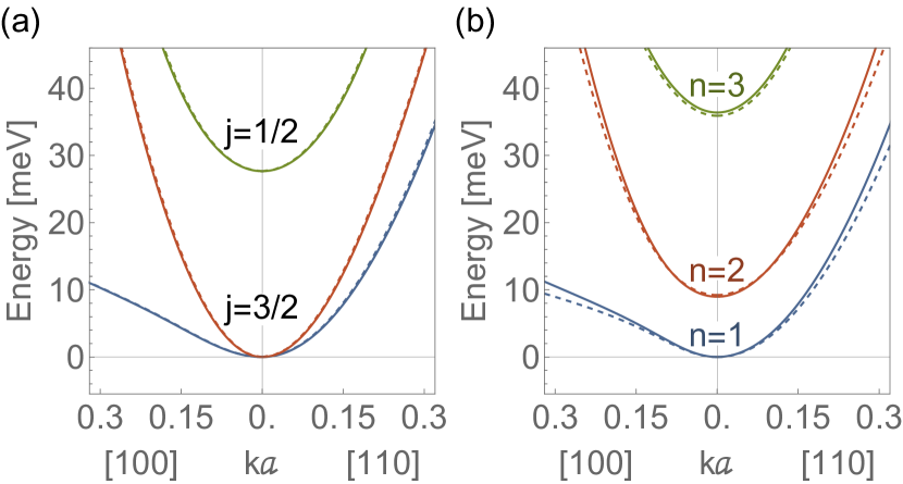
Figure 1: Low energy band structure of STO in the (a) cubic state and (b) tetragonal state. Dashed lines are computed from DFT and full lines the tight-binding model in Eq. (1). The momenta in (a) and (b) are along the cubic and pseudocubic directions respectively, and $a$ is the cubic lattice constant.

II.2 Minimal electronic model

A minimal tight-binding model with the $3d$ $t_{2g}$ orbitals of the Ti atom $yz$, $zx$ and $xy$, denoted respectively $\mu=x,y$, and $z$ in this work, successfully describes the low-energy electronic band dispersion (full lines in Fig. 1) in both cubic and tetragonal phases [56, 57, 58, 17, 30]. The non-interacting model Hamiltonian reads,

$$\mathcal{H}=\mathcal{H}_{0}+\mathcal{H}_{\mathrm{SOC}}+\mathcal{H}_{\mathrm{AFD}}.$$ (1)

Here, we have included a hopping term up to next-nearest neighbors,

$$\mathcal{H}_{0}=\sum_{\bm{k}s\mu\nu}t_{\mu\nu}(k)c^{\dagger}_{\mu s}(\bm{k})c_{\nu s}(\bm{k})$$ (2)

between orbitals $\mu$ and $\nu$ with spin $s=\pm 1/2$ (shorthanded as $s=\pm$ in operator labels as in $c^{\dagger}_{\mu+}$). The atomic SOC of the $t_{2g}$ manifold reads,

$$\mathcal{H}_{\mathrm{SOC}}=-2\xi\bm{l}\cdot\bm{s}$$ (3)

where we introduced an effective orbital moment operator with $l=1$ [59, 60, 61]. The physical orbital angular momentum $\bm{l}(t_{2g})$ is directed in the opposite direction with respect to ${\bm{l}}$.

Finally, the tetragonal crystal field term is,

$$\mathcal{H}_{\mathrm{AFD}}=\Delta\sum_{\mu s}\delta_{\mu,z}c^{\dagger}_{\mu s}c_{\mu s}$$ (4)

which effectively accounts for the AFD distortion by shifting the energy of the $\mu=z$ orbital [30].

The $t_{2g}$ hopping term reproduces the low-energy quadratic dispersion given by DFT along the high-symmetry cubic directions [Fig. 1(a)],

$$t_{\mu\mu}(\bm{k})= -2t_{1}\left(\cos k_{\alpha}+\cos k_{\beta}\right)-2t_{2}\cos k_{\mu}$$

$$-4t_{3}\cos k_{\alpha}\cos k_{\beta}+(4t_{1}+2t_{2}+4t_{3})$$ (5)

$$t_{\mu\nu}(\bm{k})= -4t_{4}\sin k_{\mu}\sin k_{\nu},$$ (6)

with hopping parameters $t_{1}=451$ meV, $t_{2}=40$ meV, $t_{3}=111$ meV and $t_{4}=27$ meV. In Eq. (5) $\alpha\neq\beta$ and $\alpha,\beta\neq\mu$, while in Eq. (6), $\mu\neq\nu$.

The eigenstates of Eq. (3) can be classified with an effective total angular momentum $\bm{j}=\bm{l}+\bm{s}$ with the associated quantum number $j$. The SOC term breaks the six-fold degeneracy of the $t_{2g}$ manifold at the zone center, opening a $3\xi=28$ meV gap between the lower multiplet $j=3/2$ and the higher doublet $j=1/2$ in the high-$T$ cubic state [Fig. 1(a)]. In terms of the $t_{2g}$ orbital operators $c^{\dagger}_{\mu s}$ these new eigenstates and associated operators, $c^{\dagger}_{j,j_{z}}$, take the following form at the zone center [60]:

$$c^{\dagger}_{\frac{3}{2},\pm\frac{3}{2}} =\mp\frac{1}{\sqrt{2}}\left(c^{\dagger}_{x,\pm}\pm ic^{\dagger}_{y,\pm}\right)$$ (7)

$$c^{\dagger}_{\frac{3}{2},\pm\frac{1}{2}} =\frac{1}{\sqrt{6}}\left(\mp c^{\dagger}_{x,\mp}-ic^{\dagger}_{y,\mp}+2c^{\dagger}_{z,\pm}\right)$$ (8)

$$c^{\dagger}_{\frac{1}{2},\pm\frac{1}{2}} =\frac{1}{\sqrt{3}}\left(-c^{\dagger}_{x,\mp}\mp ic^{\dagger}_{y,\mp}\mp c^{\dagger}_{z,\pm}\right).$$ (9)

The tetragonal crystal field term $\mathcal{H}_{\mathrm{AFD}}$ in Eq. (1), does not affect $j_{z}=\pm 3/2$ states which remain therefore eigenstates of the full Hamiltonian at the zone center. Instead, it mixes states with $j_{z}=\pm 1/2$ (i.e. states with non-zero $\mu=z$ orbital character) and thus splits the degeneracy of the lowest multiplet $j=3/2$ at the zone center. A fitting to the DFT band structure in the low-$T$ tetragonal phase [Fig. 1(b)] gives $\Delta=17.7$ meV, and sets the following order of the three doubly-degenerate bands at $\Gamma$:

$$c^{\dagger}_{1,\pm} =c^{\dagger}_{\frac{3}{2},\mp\frac{3}{2}}$$ (10)

$$\mathcal{E}_{1} =0$$

$$c^{\dagger}_{2,\pm} =\cos\theta c^{\dagger}_{\frac{3}{2},\pm\frac{1}{2}}\mp\sin\theta c^{\dagger}_{\frac{1}{2},\pm\frac{1}{2}}$$ (11)

$$\mathcal{E}_{2} =\frac{1}{2}\left(3\xi+\Delta-\sqrt{9\xi^{2}-2\xi\Delta+\Delta^{2}}\right)$$

$$c^{\dagger}_{3,\pm} =\pm\sin\theta c^{\dagger}_{\frac{3}{2},\pm\frac{1}{2}}+\cos\theta c^{\dagger}_{\frac{1}{2},\pm\frac{1}{2}}$$ (12)

$$\mathcal{E}_{3} =\frac{1}{2}\left(3\xi+\Delta+\sqrt{9\xi^{2}-2\xi\Delta+\Delta^{2}}\right)$$

from lowest to highest energy $\mathcal{E}_{1}<\mathcal{E}_{2}<\mathcal{E}_{3}$, and with $\tan 2\theta=\frac{-2\sqrt{2}\Delta}{-\Delta+9\xi}$. Note that the pseudospin index $\pm$ of the bands in Eqs. (10)-(12) is chosen to coincide with the projection of the electronic spin along the real orbital moment instead of the effective orbital moment within the T-P equivalence [61] ($\bm{l}(t_{2g})=-\bm{l}$, see also [62]).

Carrying the analysis for general momentum we can write the electronic Hamiltonian Eq. (1) in the absence of a polar distortion as

$$\mathcal{H}=\sum_{n\bm{k}}\psi_{n}^{\dagger}(\bm{k})\mathcal{E}_{n}(\bm{k})\sigma_{0}\psi_{n}(\bm{k})$$ (13)

where we defined the spinor $\psi^{\dagger}_{n}=(c^{\dagger}_{n+},c^{\dagger}_{n-})$ for band $n$, and introduced the $2\times 2$ identity matrix $\sigma_{0}$ for pseudospin degeneracy. Figure 1(b) shows that this model with the parameters quoted above gives an excellent fit of the bands obtained by DFT in the presence of both AFD and SOC.

III Polar soft mode in STO

Figure 2: Atomic distortions of the $E_{u}$ irrep for $Ima2$ ($C_{2v}$) with polar axis $\bm{\hat{n}}_{p}\parallel[1\bar{1}0]$ for basis modes (a) $\bar{S}_{1}$, (b) $\bar{S}_{2}$, (c) $\bar{S}_{3}$, (d) $\bar{S}_{4}$ and (e) $\bar{S}_{5}$ given by Eqs. (15)-(19) and Table 1. In all cases distortions are on the plane of the drawing and the arrowheads identify the atoms moving. The left inset shows the pseudocubic and tetragonal in-plane axes. The Wickoff positions of Ti, O_x and O_y atoms are given in [62]. The atomic displacements for the basis of $A_{2u}$ mode with polar axis $\bm{\hat{n}}_{p}\parallel[001]$ are equivalent to panels (a)-(c) with all displacements pointing out of the plane, i.e. rotated by $\pi/2$ around the $b_{t}$ tetragonal axis.

Although we are focusing on the temperature region where an AFD is present, it is customary to discuss the atomic displacements of the near zone-center polar soft mode in terms of a complete set of basis modes defining symmetry coordinates for the $T_{1u}$ irrep of $O_{h}$ in the high-$T$ cubic phase. Indeed, Axe [63] introduced one such possible set of coordinates to describe the eigenvectors of polar normal modes in cubic perovskite structures, which has been used to restrict the possible atomic distortions of the various polar modes that were compatible with reflectivity [63], neutron scattering [64] and hyper-Raman experiments [65]. Since this coordinate set has been widely used and referred to in the literature of polar modes in STO, we shall use it in our work as well. Within this framework, a general polar distortion can be decomposed into symmetry coordinates in the following way

$$\bm{\bar{U}}=(\bm{r}^{\mathrm{Sr}},\bm{r}^{\mathrm{Ti}},\bm{r}^{\mathrm{O}_{x}},\bm{r}^{\mathrm{O}_{y}},\bm{r}^{\mathrm{O}_{z}})=\sum_{i}\bm{\hat{n}}_{i}u_{i}\bar{S}_{i}.$$ (14)

Here, $\bm{\hat{n}}_{i}$ is a unit vector setting the direction of atomic displacements for basis mode $i$. We shall see that, in general, displacements with the same polar axis, $\bm{\hat{n}}_{p}$, do not need to be collinear; this requires a different $\bm{\hat{n}}_{i}$ for each basis mode. $\bar{S}_{i}$ defines the basis of eigenmodes expressed in terms of collinear atomic displacements $(s^{\mathrm{Sr}},s^{\mathrm{Ti}},s^{\mathrm{O}_{x}},s^{\mathrm{O}_{y}},s^{\mathrm{O}_{z}})$,

$$\bar{S}_{1} =\frac{1}{1+\kappa_{1}}(0,-\kappa_{1},1,1,1)$$ (15)

$$\bar{S}_{2} =\frac{1}{1+\kappa_{2}}(-\kappa_{2},1,1,1,1)$$ (16)

$$\bar{S}_{3} =\frac{2}{3}(0,0,-\frac{1}{2},-\frac{1}{2},1)$$ (17)

and shown in Figs. 2(a)-(c). The coefficients $\kappa_{1}=\frac{3m^{\mathrm{O}}}{m^{\mathrm{Ti}}}$ and $\kappa_{2}=\frac{3m^{\mathrm{O}}+m^{\mathrm{Ti}}}{m^{\mathrm{Sr}}}$ ensure the center of mass is not displaced for any of the $\bar{S}_{i}$ modes. That is, $\sum_{j}m^{j}\bm{r}^{j}=0$ when summing over all the $j$ atoms with atomic mass $m^{j}$ and displacement $r^{j}=u_{i}s^{j}$ in the unit cell for each of the $\bar{S}_{i}$ modes. The coefficient $u_{i}$ sets the amplitude of basis mode $i$ in the general displacement $\bm{\bar{U}}$. The $\bar{S}_{i}$ modes in Eqs. (15)-(17) have been normalized so that their amplitude $u_{i}$ is equal to the relative displacement of the two bodies in the mode. For instance, $u_{1}$ is the relative atomic displacement between Ti and the O cage in the $\bar{S}_{1}$ mode, $r^{\mathrm{O}}-r^{\mathrm{Ti}}=u_{1}(s_{1}^{\mathrm{O}}-s_{1}^{\mathrm{Ti}})=u_{1}$. Similarly, $u_{2}$ is the relative displacement between Sr and the Ti-O cage in mode $\bar{S}_{2}$. This normalization reduces the two-body problem into a one-body problem with a reduced mass when deriving the electron-phonon Hamiltonian, as will be shown in Section V. Note the bar symbol indicates a vector spanned by the atoms of the unit cell (as in $\bar{S}_{i}$), whereas the vector referring to the Cartesian coordinates of the atomic displacements is specified by bold notation (as in $\bm{\hat{n}}_{i}$).

As it is well known, the long-range Coulomb interaction partially lifts the three-fold degeneracy of polar modes into a high-energy longitudinal mode and low-energy doubly degenerate transverse modes [66]. Thus, the soft mode of STO is transverse and, in general, it is a linear combination of all three $\bar{S}_{i}$ modes. According to several studies [66, 63, 64, 65], its atomic displacements are close to the $\bar{S}_{1}$ mode [Eq. (15)], also known as the Slater mode [67], where the Ti atom vibrates opposite to the O octahedron [see Fig. 2(a)]. Because of the strong sensitivity of the electron-phonon coupling to the soft-mode eigenvector, we anticipate that even a small deviation from a pure Slater mode can have important consequences for superconductivity.

Rigorously speaking, the above analysis in terms of three basis modes is only valid in the cubic phase. The presence of the AFD distortion requires an enlargement of the basis. Indeed, below $105$ K, as the symmetry of STO is lowered to a tetragonal structure belonging to the $I4/mcm$ space group ($D_{4h}$ point group), the $T_{1u}$ polar mode of the cubic state splits into: (a) a $A_{2u}$ irrep with a polar axis along $[001]$ ($C_{4v}$) and (b) a $E_{u}$ irrep with a polar axis perpendicular to $[001]$. This split of the soft mode has been tracked in $T$ by hyper-Raman spectroscopy [68]: $\hbar\omega_{E_{u}}\sim 1$ meV and $\hbar\omega_{A_{2u}}\sim 2$ meV at 7K.

The analysis of polar modes for case (a) is simpler, as the basis of symmetry modes Eqs. (15)-(17) for the $T_{1u}$ mode of $O_{h}$ in the high-$T$ cubic phase is also a complete basis for the $A_{2u}$ mode in the low-$T$ tetragonal phase. Therefore, in this case an enlargement of the basis is not needed. Of course, the atomic displacements are restricted along the tetragonal $z$ axis for this irrep, $\hat{n}_{i}^{A_{2u}}\parallel[001]$, leading to a polar tetragonal structure with $I4cm$ lower symmetry. Although here we will focus on the paraelectric phase, we note that the out-of-plane polar mode has also been observed by electron microscopy and optical second harmonic generation in strained STO films in the symmetry broken polar phase  [69, 70, 71, 5] highlighting the relevance of this symmetry.

For case (b), in general, we notice that a distortion belonging to the $E_{u}$ irrep can lead to various lower-symmetry structures ($Ima2$, $Fmm2$ or $Cm$), all of which have a polar axis perpendicular to the tetragonal axis $[001]$. Here we will focus on $Ima2$ ($C_{2v}$), a space group with a polar axis parallel to the tetragonal in-plane axis, i.e. along the pseudocubic direction $[1\bar{1}0]$ (see Fig. 2). This choice is justified by the fact that this mode has been experimentally reported in the ferroelectric phase of isotope O₁₈ and Ca substitution systems [72, 73] and the optically excited metastable polar phase of STO [74]. Because the in-plane O atoms are not equivalent in $Ima2$, and Ti and in-plane O atoms are allowed to move orthogonally to the polar axis, the dimension of the basis symmetry modes has to be expanded to five. That is, besides the three $\bar{S}_{i}$ modes presented in Eqs. (15)-(17), with displacements along the polar axis (i.e. $\bm{\hat{n}}_{i}=\bm{\hat{n}}_{p}\parallel[1\bar{1}0]$ for $i=1,2,3$) one needs to add to the subspace another two $\bar{S}_{i}$ modes with an amplitude along the perpendicular direction (i.e. $\bm{\hat{n}}_{i}\parallel[110]\perp\bm{\hat{n}}_{p}$ for $i=4,5$) to obtain a complete basis,

$$\bar{S}_{4} =\frac{1}{2}(0,1,0,0,0),$$ (18)

$$\bar{S}_{5} =\frac{1}{2}(0,0,1,-1,0).$$ (19)

These two modes are shown in Figs. 2(d) and 2(e), respectively.

In general, normal modes will not be made of collinear displacements. Still, they can be decomposed into the present basis, with each element representing collinear displacements. Indeed, different elements of the expansion can have displacements in different directions although they contribute to the same polarization vector.

Table 1 summarizes the polar distortion directions $\bm{\hat{n}}_{i}$ of the different $\bar{S}_{i}$ for both the $E_{u}$ ($Ima2$) and $A_{2u}$ ($I4cm$) modes we will consider throughout this work.

In general for a mode $i$ with displacement amplitude $u_{i}$ and associated with the polarization vector $\bm{\hat{n}}_{p}$, irrespectively of the direction of atomic displacements, we define its associated polarization vector as

$$\bm{u}_{i}=u_{i}\bm{\hat{n}}_{p}.$$ (20)

Notice that formally $\bm{u}_{i}$ should be multiplied by an effective charge to be a real polarization. On the other hand, such charge does not play any role in the present context and will be omitted.

Near the zone center but for finite $\bm{q}$ it is important to consider the long-range Coulomb interaction which will split transverse and longitudinal modes. In this case we will restrict to the symmetrized modes $i=1,2,3$ and we will assume that for $\bm{q}$ along an arbitrary direction we can decompose mode $i$ into the set of the same $i$ modes along directions defined by ${\bm{q}}$ as done in Ref. [30] for the Slater mode. For simplicity, deviations of the polarization vector from pure longitudinal or transverse directions due to non-spherical symmetry will be neglected. In this way we can generalize Eq. (20) to

$$\bm{u}_{i}(\bm{q})=u_{i}(\bm{q})\bm{\hat{n}}_{p}(\bm{q}),$$ (21)

which will be used next to discuss the general interaction with polar modes.

Table 1: Symmetry coordinates of polar $E_{u}$ and $A_{2u}$ modes for a general distortion $\bm{\bar{U}}=\sum_{i}u_{i}\bm{\hat{n}}_{i}\bar{S}_{i}$ in the tetragonal phase of STO. The atomic displacement coordinates $\bar{S}_{i}$ are given by Eqs. (15)-(19). The polar axis of the modes shown here is along the in-plane direction, $\bm{\hat{n}}^{E_{u}}_{p}\parallel[1\bar{1}0],[110]$, for $E_{u}$ modes and out-of-plane $\bm{\hat{n}}^{A_{2u}}_{p}\parallel[001]$ for $A_{2u}$ modes. The symmetry modes analysis has been performed using the ISODISTORT tool [75, 76].

Irrep (space group, point group)	$\bm{\hat{n}}_{p}$	$\bm{\hat{n}}_{i}$	$\bar{S}_{i}$
$E_{u}$ ($Ima2$, $C_{2v}$)	$[1\bar{1}0]$	$[1\bar{1}0]$	$\bar{S}_{1}$, $\bar{S}_{2}$, $\bar{S}_{3}$
	$[1\bar{1}0]$	$[110]$	$\bar{S}_{4}$, $\bar{S}_{5}$
	$[110]$	$[110]$	$\bar{S}_{1}$, $\bar{S}_{2}$, $\bar{S}_{3}$
	$[110]$	$[1\bar{1}0]$	$\bar{S}_{4}$, $\bar{S}_{5}$
$A_{2u}$ ($I4cm$, $C_{4v}$)	$[001]$	$[001]$	$\bar{S}_{1}$, $\bar{S}_{2}$, $\bar{S}_{3}$

IV Linear Rashba-like coupling

IV.1 Ab initio computation of couplings

Having established the electronic structure of STO in Sec. II and the relevant polar phonon modes around the zone center in Sec. III, in this section we proceed to study and estimate their coupling to linear order. In particular, we will show how a symmetry allowed linear coupling to transverse TO modes emerges naturally from induced hopping channels, and estimate the corresponding coupling constant for all electronic bands with the aid of ab initio frozen-phonon results in tetragonal STO.

The linear coupling Hamiltonian between a polar distortion and electronic bands [Eqs. (10)-(13)] can be expressed as

$$\mathcal{H}_{u}=\sum_{nn^{\prime}\bm{k}\bm{q},\bar{S}_{i}}\psi_{n}^{\dagger}(\bm{k}+\frac{\bm{q}}{2})\bm{\Lambda}^{\bar{S}_{i}}_{nn^{\prime}}(\bm{k},\bm{q})\psi_{n^{\prime}}(\bm{k}-\frac{\bm{q}}{2})$$ (22)

with the coupling $2\times 2$ matrix $\bm{\Lambda}^{\bar{S}_{i}}_{nn^{\prime}}(\bm{k},\bm{q})$ in pseudospin space for a polar mode $\bar{S}_{i}$. The intra-band ($n^{\prime}=n$) coupling matrix has the following form to linear order in $\bm{k}$ and $u_{\alpha}$ in a $D_{4h}$ point group:

$$\bm{\Lambda}^{\bar{S}_{i}}_{nn}(\bm{k},\bm{q})= ka\varepsilon_{\alpha\beta\gamma}u_{\alpha}\hat{k}_{\beta}\sigma_{\gamma}\left(\delta_{\alpha z}\tau^{\bar{S}_{i}}_{n,C}+\delta_{\beta z}\tau^{\bar{S}_{i}}_{n,B}+\delta_{\gamma z}\tau^{\bar{S}_{i}}_{n,A}\right)$$

$$= ka\Bigl{[}\tau^{\bar{S}_{i}}_{n,A}(\hat{k}_{y},-\hat{k}_{x},0)\sigma_{z}+\tau^{\bar{S}_{i}}_{n,B}\hat{k}_{z}(-\sigma_{y},\sigma_{x},0)$$ (23)

$$+\tau^{\bar{S}_{i}}_{n,C}(0,0,\hat{k}_{x}\sigma_{y}-\hat{k}_{y}\sigma_{x})\Bigr{]}\cdot\bm{u}_{i}(\bm{q}),$$

where $a$ is the lattice constant, $\varepsilon_{\alpha\beta\gamma}$ the Levi-Civita symbol, $\delta_{\alpha\beta}$ the Kronecker’s delta-function, $\hat{k}_{i}=\bm{\hat{k}}\cdot\bm{\hat{\imath}}$ the Cartesian projection of the unitary momentum vector, and $\sigma_{j}$ the Pauli matrices for the pseudospin of the electronic bands. We also defined the couplings $\tau^{\bar{S}_{i}}_{n,l}$ with symmetry allowed irrep labels $l=A,B,C$.

Equation (IV.1) describes a Rashba-like linear-in-$k$ coupling between a polar distortion $\bm{u}_{i}(\bm{q})=u_{i}(\bm{q})\bm{\hat{n}}_{p}(\bm{q})$ of mode $\bar{S}_{i}$ and the electronic band $n$ with pseudospin $\bm{\sigma}$. The first form in Eq. (IV.1) makes evident that $z$ is a privileged axis in this structure and clarifies the meaning of the $\tau^{\bar{S}_{i}}_{n,l}$ coefficients which are associated with one member of the triad $(\bm{u}_{i},\bm{k},\bm{\sigma})$ having a projection on the $z$-direction.

In the following we drop the index $\bar{S}_{i}$ from the couplings $\tau_{n,l}$ for simplicity, but emphasize that these couplings vary a lot from mode to mode. The Rashba matrix Eq. (IV.1) has the most general form allowed by the symmetry of our tetragonal system to linear order in $\bm{k}$. It consists of couplings $\tau_{n,A}$ and $\tau_{n,B}$ ($\tau_{n,C}$) which couple to the corresponding $E_{u}$ ($A_{2u}$) modes with polar axis $\bm{\hat{n}}_{p}$ in the $xy$ plane (along the $z$ axis). These parameters are not related by symmetry, and we will estimate them using ab initio computations in the following. Note that in higher cubic symmetry Eq. (IV.1) simplifies to $ka[\tau^{\bar{S}_{i}}_{n}\bm{\hat{k}}\times\bm{\sigma}]\cdot\bm{u}(\bm{q})$ [44, 27, 28].

The interband coupling matrices ($n^{\prime}\neq n$) in Eq. (22) have a similar $k$-linear Rashba form. However, because we are considering a long-wavelength $\bm{q}\rightarrow 0$ phonon, the inter-band terms result in $k$-cubic Rashba intra-band terms upon perturbation. We therefore focus solely on intra-band terms with $n^{\prime}=n$ [Eq. (IV.1)] in this work, which involve $k$-linear Rashba terms which can be directly extracted from ab initio frozen-phonon computations.

Finite Rashba couplings $\tau_{n,l}$ in Eq. (IV.1) cause the characteristic linear-in-$k$ band splitting $E_{n+}(\bm{k})-E_{n-}(\bm{k})\equiv\delta E_{n}(\bm{k})$. From the Rashba coupling matrix Eq. (IV.1) the splitting for band $n$ is generally given by the following expression

$$\delta E_{n} (\bm{k},\bm{u}_{i}(\bm{q}))=2kau_{i}(\bm{q})\times$$

$$\times\sqrt{\tau_{n,A}^{2}\left(\hat{k}_{y}\hat{n}_{px}-\hat{k}_{x}\hat{n}_{py}\right)^{2}+\tau_{n,B}^{2}\hat{k}_{z}^{2}\left(\hat{n}_{px}^{2}+\hat{n}_{py}^{2}\right)+\tau_{n,C}^{2}\left(\hat{k}_{x}^{2}+\hat{k}_{y}^{2}\right)\hat{n}_{pz}^{2}-2\tau_{n,B}\tau_{n,C}\left(\hat{k}_{x}\hat{n}_{px}+\hat{k}_{y}\hat{n}_{py}\right)\hat{k}_{z}\hat{n}_{pz}},$$ (24)

which peaks (vanishes) along momenta $\bm{k}$ perpendicular (parallel) to the polar axis $\bm{\hat{n}}_{p}$ of the mode. As we show in the following, one can use this band split to extract the Rashba couplings of each band $\tau_{n,l}$ to each mode $\bar{S}_{i}$. For this purpose, we need to particularize Eq. (IV.1) for the direction given by the polar axis of the polar modes. We obtain the following pseudospin split for a mode $\bar{S}_{i}$

$$\frac{\delta E_{n}(\bm{k},u_{i}[1\bar{1}0])}{2u_{i}} =ka\sqrt{\frac{\tau_{n,A}^{2}}{2}(\hat{k}_{y}+\hat{k}_{x})^{2}+\tau_{n,B}^{2}\hat{k}_{z}^{2}}$$ (25)

$$\frac{\delta E_{n}(\bm{k},u_{i}[001])}{2u_{i}} =ka\tau_{n,C}\sqrt{\hat{k}_{x}^{2}+\hat{k}_{y}^{2}}$$ (26)

with an amplitude $u_{i}$ and a polar axis $\bm{\hat{n}}_{p}\parallel[1\bar{1}0]$ and $\bm{\hat{n}}_{p}\parallel[001]$, respectively.

To obtain the couplings $\tau_{n,l}$, we computed by first principles the reconstructed electronic band structure of tetragonal STO in the presence of a frozen phonon $\bm{u}_{i}(\bm{q}=0)$ for all $\bar{S}_{i}$ modes listed in Table 1 for both $E_{u}$ and $A_{2u}$ irreps.

Frozen-phonon distorted structures have been constructed by displacing atoms along each symmetrized mode while keeping fixed the optimized lattice parameters. In order to identify the linear regime in $\bm{u}_{i}$, band-structure calculations have been performed for several values of the displacement amplitude up to 0.1 Å. By fitting the linear-$k$ regime of the DFT band-splitting in Fig. 3 along various momentum directions, we can obtain for each band $n$ the $E_{u}$ Rashba couplings $\tau_{n,A}$ and $\tau_{n,B}$, and the $A_{2u}$ coupling $\tau_{n,C}$. The sign of these couplings is extracted from the averaged spin-polarization values of each band obtained from the same ab initio computation. Keeping track of these signs is very important when computing the coupling to a mode that is combination of the $\bar{S}_{i}$ modes, as will become clear below.

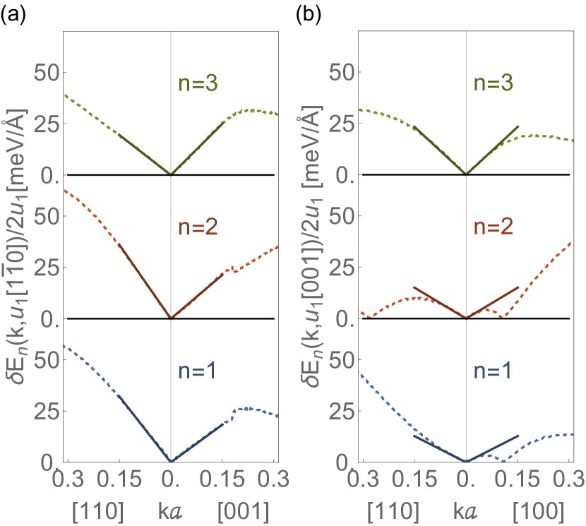
Figure 3: Electronic band split $\delta E_{n}\left(\bm{k},u_{1}(q=0)\bm{\hat{n}}_{p}\right)$ in the presence of a frozen Slater polar mode [Eq. (15)] normalized by twice the amplitude $2u_{1}$ along the specified $\bm{k}$ directions for the three bands of tetragonal STO [Fig. 1(b)]. The polar axis of the mode is along (a) $\bm{\hat{n}}_{p}^{E_{u}}\parallel[1\bar{1}0]$ and (b) $\bm{\hat{n}}_{p}^{A_{2u}}\parallel[001]$ in pseudocubic coordinates. Dashed lines are ab initio results from frozen-phonon distortions. Full lines are the $k$-linear Rashba split model Eq. (25) in (a) and Eq.(26) in (b), up to $ka=0.15$. All shown $\bm{k}$ directions are perpendicular to the polar axis $\bm{\hat{n}}_{p}$.

As an example, we show the results of the frozen Slater mode $\bar{S}_{1}$ [Eq. (15) and Fig. 2(a)]. The resulting band split of each $n$ band $\delta E_{n}(\bm{k})$ found by ab initio is shown by the dashed lines in Fig. 3(a) and Fig. 3(b), for $\bm{u}_{1}$ with a polar axis along the in-plane $\bm{\hat{n}}_{p}\parallel[1\bar{1}0]$ ($E_{u}$ mode) and out-of-plane $\bm{\hat{n}}_{p}\parallel[001]$ ($A_{2u}$ mode) pseudocubic directions, respectively. As seen in Fig. 3, for small enough momenta all bands show a linear-$k$ split (full lines), but the momentum amplitude beyond which deviations of $k$-linearity become significant depends on the band, the polar axis and the direction of momentum. In fact, while for the $E_{u}$ mode the split is robustly linear around the zone center with small deviations beyond $ka\sim 0.2$, for the $A_{2u}$ mode strong non-linear features appear already at small $ka\sim 0.05$ for the two lowest bands. This highlights the limitation of a conventional Rashba linear-$k$ model Eq. (IV.1) to describe the coupling between the bands and some of the polar modes in this system. We will come back to this important point in Section VI.

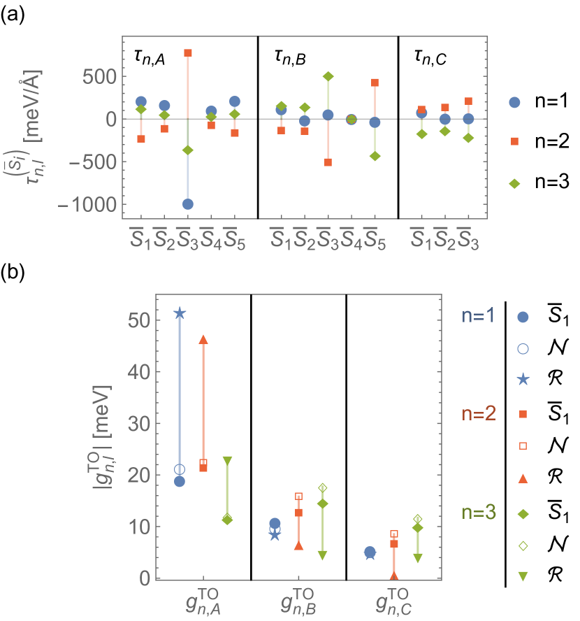
Figure 4: (a) $k$-linear Rashba couplings $\tau_{n,A}$, $\tau_{n,B}$ and $\tau_{n,C}$ in Eq. (IV.1) in meV/$\AA$ for band $n$ and mode $\bar{S}_{i}$ [Eqs. (15)-(19)] in tetragonal STO. They were obtained from fits of the spin-split Eqs (25)-(26) to frozen phonon ab initio results. The numerical values are listed in [62]. (b) Absolute value of the estimated electron-FE-mode Rashba couplings [Eq. (34)] for band $n$ for three possible eigenvectors of the FE mode: a pure $\bar{S}_{1}$ mode, eigenvector from neutron data [Eq. (36)] and from Raman data [Eq. (37)]. We have used experimental optical gaps $\hbar\omega^{E_{u}}_{\mathrm{TO}}=1$ meV and $\hbar\omega^{A_{2u}}_{\mathrm{TO}}=2$ meV, and electronic momentum $k_{F}a=0.3$.

The Rashba couplings to the rest of the $\bar{S}_{i}$ modes belonging to $E_{u}$ and $A_{2u}$ irreps (see Table 1) have been also estimated by the same fitting procedure to frozen phonon ab initio computations; they are shown together with those of the Slater mode in Fig. 4(a) (also listed in [62]). As seen, for all $\bar{S}_{i}$ modes the $E_{u}$ coupling $\tau_{n,A}$ is larger in the lowest two bands ($n=1,2$) than the highest band ($n=3$). This hierarchy is reversed for the couplings $\tau_{n,B}$ and $\tau_{n,C}$ where the highest two bands ($n=2,3$) show larger couplings than the lowest band ($n=1$). Remarkably, the Rashba coupling to the $\bar{S}_{3}$ mode, with apical oxygen atoms O_z moving opposite to in-plane O atoms O_x,y distorting the octahedra [see Eq. (17) and Fig. 2(c)] can be an order of magnitude larger than the other couplings. As we will show in the following section, this gigantic Rashba coupling has important consequences for the electron coupling to the soft mode. Indeed, an enlarged electron-phonon coupling follows from a modest contribution of $\bar{S}_{3}$ to any polar mode.

IV.2 Real-space origin of the coupling

We will now show how the symmetry allowed coupling Eq. (IV.1) emerges when considering microscopic processes in real space. In the presence of a polar distortion $\bm{\bar{U}}=\sum_{i}u_{i}\bm{\hat{n}}_{i}\bar{S}_{i}$ of the lattice, new terms are allowed in the Hamiltonian Eq. (1) for $t_{2g}$ electrons around the zone center. These new terms include effects such as the polarization of the orbitals and induced hopping channels which are symmetry forbidden in the absence of the distortion [47, 77, 58, 78, 30, 39]. We thus consider the following Hamiltonian with the spinor of the $t_{2g}$ orbitals $\psi^{\dagger}_{\mu}=(c^{\dagger}_{\mu+},c^{\dagger}_{\mu-})$,

$$\mathcal{H}_{u}=\sum_{\bm{k}\bm{q}\mu\nu j}\psi^{\dagger}_{\mu}(\bm{k}+\frac{\bm{q}}{2})t_{\mu\nu j}(\bm{k},\bm{q})\sigma_{j}\psi_{\nu}(\bm{k}-\frac{\bm{q}}{2})+\mathrm{h.c.}$$ (27)

which describes the induced hopping between a $d$-orbital $\mu$ and a nearest neighbor $d$-orbital $\nu$. The Pauli matrices $\sigma_{j}$ represent spin-independent ($j=0$) as well as spin-dependent ($j=x,y,z$) hopping processes. Fig. 5 shows some examples for $j=0,x$ and $y$. Around the zone center ($\bm{k}\rightarrow 0$, $\bm{q}\rightarrow 0$), the new allowed terms have the following form

$$t_{\mu\nu j}(\bm{k},\bm{q})\approx\sum_{ilm}\frac{\partial t_{\mu\nu j}}{\partial u_{i,l}(\bm{q})}u_{i,l}(\bm{q})k_{m}a$$ (28)

to linear order in the polar distortion $\bm{u}_{i}(\bm{q})=u_{i}(\bm{q})\bm{\hat{n}}_{p}(\bm{q})$ for a mode $\bar{S}_{i}$ with amplitude $u_{i,l}(\bm{q})$ in Cartesian coordinate $l$, and polar axis $\bm{\hat{n}}_{p}$. In the case of tetragonal STO, as discussed in the previous section, the polar axis we are considering are the in-plane $\bm{\hat{n}}^{E_{u}}_{p}\parallel[1\bar{1}0]$ for $E_{u}$ modes and out-of-plane $\bm{\hat{n}}^{A_{2u}}_{p}\parallel[001]$ for $A_{2u}$ modes in pseudocubic coordinates. In general, the precise form of the terms allowed in Eq. (28) is set by symmetry; and thus it depends on the pair of orbitals $\mu$ and $\nu$ involved, as well as the direction of the polar axis $\bm{\hat{n}}_{p}$ associated with the distortion $\bm{\bar{U}}$.

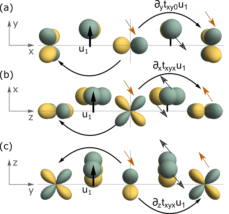
Figure 5: Induced inter-orbital hopping elements in Eq. (29) between $d$-orbital $\nu=y$ with spin $\downarrow$ (orange arrow) at the origin and $d$-orbital $\mu=x$ with spin $s$ (orange arrow) at neighboring Ti atoms, mediated by the $p$-orbitals with spin $s^{\prime}$ (gray arrow) in the bridging oxygens. (a) Spin-conserving process $\partial_{y}t_{xy0}u_{1}$ with $s=\downarrow$ mediated by $|p_{z}\downarrow>$. Spin-flip processes $s=\uparrow$ when allowing for SOC of the oxygen $\xi_{O}$ for (b) $\partial_{x}t_{xyx}u_{1}$ mediated by $|p_{z}\downarrow>$ and $|p_{y}\uparrow>$ with matrix-element $i\xi_{O}$, and (c) $\partial_{z}t_{xyx}u_{1}$ mediated by $|p_{x}\downarrow>$ and $|p_{z}\uparrow>$ with matrix-element $\xi_{O}$. All three hopping elements change sign along the horizontal bond (black curved arrows) with a finite polar Slater displacement $\bm{u}_{1}$ along the vertical axis, specified in each panel. The spins on the negative horizontal axis, not shown for clarity, are mirror symmetric with respect to those shown on the positive side.

As a concrete example, we explicitly consider in the following the case of $\mu=x$ and $\nu=y$ orbitals. The lowest electronic band in the tetragonal state ($n=1$) is formed by only these two orbitals at the zone center [see Eq. (10)], and thus induced hopping amplitudes involving these two orbitals are the relevant terms for the coupling of the lowest band to polar modes. For a general polarization vector defined by Eq. (21), for mode $\bar{S}_{i}$, the following inter-orbital hopping elements are allowed in Eq. (27):

$$\sum_{j}t_{xyj}(\bm{k},\bm{q})\sigma_{j} \approx 2i\partial_{x}t_{xy0}u_{i}(\bm{q})ka\bigl{[}-\hat{k}_{y}\hat{n}_{px}+\hat{k}_{x}\hat{n}_{py}\bigr{]}\sigma_{0}$$

$$+2\partial_{x}t_{xyx}u_{i}(\bm{q})ka\bigl{[}-\hat{n}_{px}\sigma_{x}+\hat{n}_{py}\sigma_{y}\bigr{]}\hat{k}_{z}$$

$$+2\partial_{z}t_{xyx}u_{i}(\bm{q})ka\bigl{[}-\hat{k}_{x}\sigma_{x}+\hat{k}_{y}\sigma_{y}\bigr{]}\hat{n}_{pz}$$ (29)

where we have used the shorthand notation $\frac{\partial t_{\mu\nu j}}{\partial u_{i,l}(\bm{q})}\equiv\partial_{l}t_{\mu\nu j}$. The first term in Eq. (29) corresponds to a spin-conserving ($\sigma_{0}$) hopping channel with amplitude $\partial_{x}t_{xy0}$ which changes sign with hopping direction, shown in Fig. 5(a). It couples only to the in-plane components of the polar distortion axis $\hat{n}_{px}$ and $\hat{n}_{py}$. The second and third terms describe spin-flip ($\sigma_{x,y}$) hopping processes instead, and couple to the in-plane component of the polar axis, through the hopping amplitude $\partial_{x}t_{xyx}$ [Fig. 5(b)], as well as to the out-of-plane component $\hat{n}_{pz}$ through the hopping amplitude $\partial_{z}t_{xyx}$ [Fig. 5(c)]. Microscopically one obtains spin-flip hopping terms by extending SOC to the bridging $p$-orbitals of the oxygen atom [as shown in Figs. 5(b)-(c)], or by considering virtual processes between the $t_{2g}$ and $e_{g}$ manifolds [78]. Each $\bar{S}_{i}$ mode will generally induce different hopping amplitudes, which then result in different couplings to the electrons. Other $t_{\mu\nu j}(\bm{k},\bm{q})$ induced hopping elements between different pairs of $t_{2g}$ orbitals in Eq. (27) can be similarly obtained.

We can now connect the symmetry allowed couplings in Eq. (IV.1), to these microscopic processes by projecting Eq. (27) to the band basis [Eqs. (10)-(12)] of the non-interacting electrons. In general each coupling element $\tau_{n,l}$ is a linear combination of the different induced hopping derivatives $\partial_{l}t_{\mu\nu j}$ allowed in Eq. (28). For instance, the induced hopping derivatives between the $x$ and $y$ orbitals considered in Eq. (29), are connected to the Rashba couplings for the lowest band $n=1$ [Eq. (10)] in the following way,

$$\tau_{1,A}=-2\partial_{x}t_{xy0};\ \tau_{1,B}=2\partial_{x}t_{xyx};\ \tau_{1,C}=-2\partial_{z}t_{xyx}.$$ (30)

Similar expressions for the other two electronic bands $n=2,3$ can also be derived following the same procedure. These expressions are more involved than the particularly simple expressions in Eq. (30) for $n=1$.

To close this section we comment on the importance of the different terms in [Eq. (30)], relevant for the coupling to the lowest band $n=1$. We see from Fig. 4(a) that for $n=1$ and for all modes $\bar{S}_{i}$ except Slater ($\bar{S}_{1}$), $\tau_{1,A}\gg\tau_{1,B},\tau_{1,C}$, implying that one can safely neglect the spin-flip induced hopping terms $\partial_{x}t_{xyx}$ and $\partial_{z}t_{xy}$ in Eq. (29). For a pure Slater mode $\bar{S}_{1}$ mode, however, $\tau_{1,A}$ is of the same order of magnitude as $\tau_{1,B}$ and $\tau_{1,C}$, hence the spin-flip processes (and the symmetry equivalent virtual processes to the $e_{g}$ manifold) are in principle not negligible. However, since the $\bar{S}_{3}$ spin-conserving coupling $\tau_{1,A}^{(\bar{S}_{3})}$ is very large, a small admixture of this mode allows to neglect spin-flip processes when considering the linear coupling between the lowest band and the polar mode.

V Electron-polar-phonon Hamiltonian

In order to obtain an electron-phonon Hamiltonian, we quantize the general atomic displacements of Eq. (14) by decomposing them into a set of normal modes $\alpha$:

$$\bm{r}^{j}(\bm{q})=\sum_{\alpha}\frac{\bm{e}^{j}_{\alpha}(\bm{q})}{\sqrt{m^{j}}}\sqrt{\frac{\hbar}{2\mathcal{N}\omega_{\bm{q}\alpha}}}\mathcal{\hat{A}}_{\bm{q}\alpha}$$ (31)

Here $\mathcal{N}$ is the number of unit cells, $\mathcal{\hat{A}}_{\bm{q}\alpha}=\hat{a}_{\bm{q}\alpha}+\hat{a}^{\dagger}_{-\bm{q}\alpha}$ is the phonon operator of mode $\alpha$ with frequency $\omega_{\bm{q}\alpha}$ and normalized eigenvector $\bm{e}^{j}_{\alpha}(\bm{q})$. To proceed, we need an analogous expression for the polarization amplitude $u_{i}$ appearing in Eqs. (21)-(IV.1). We write the ansatz,

$$u_{i}=\sum_{\alpha}\frac{\varphi_{\alpha i}}{\sqrt{m_{u}}}\sqrt{\frac{\hbar}{2\mathcal{N}\omega_{\bm{q}\alpha}}}\mathcal{\hat{A}}_{\bm{q}\alpha}$$

with $m_{u}$ the atomic mass constant. Inserting it in Eq. (14) one obtains that the coefficients $\varphi_{\alpha i}$ are determined by the decomposition of the normalized displacement vector in the complete basis of the $\bar{S}_{i}$ modes [Eqs. (15)-(19)]:

$$\sqrt{m_{u}}\left(\frac{\bm{e}^{\mathrm{Sr}}_{\alpha}}{\sqrt{m^{\mathrm{Sr}}}},\frac{\bm{e}^{\mathrm{Ti}}_{\alpha}}{\sqrt{m^{\mathrm{Ti}}}},\frac{\bm{e}^{\mathrm{O_{x}}}_{\alpha}}{\sqrt{m^{\mathrm{O}}}},\frac{\bm{e}^{\mathrm{O_{y}}}_{\alpha}}{\sqrt{m^{\mathrm{O}}}},\frac{\bm{e}^{\mathrm{O_{z}}}_{\alpha}}{\sqrt{m^{\mathrm{O}}}}\right)$$

$$=\sum_{i}\varphi_{\alpha i}\hat{\bm{n}}_{i}\bar{S}_{i}$$ (32)

with $\varphi_{\alpha i}$ set to normalize the polarization eigenvector of the $\alpha$ mode, i.e. $\sum_{j}|\bm{e}^{j}_{\alpha}|^{2}=1$. As mentioned before, for a given mode $\alpha$, displacements do not need to be collinear even though they concur to the same polar axis $\bm{\hat{n}}_{p}^{\alpha}$.

With the above quantization, we obtain the following electron-polar-phonon Hamiltonian for a mode $\alpha$

$$\mathcal{H}_{u}=\frac{1}{\sqrt{\mathcal{N}}}\sum_{n\bm{k}\bm{q}\alpha}\psi_{n}^{\dagger}(\bm{k}+\frac{\bm{q}}{2})g^{\alpha}_{n}(\bm{k},\bm{q})\psi_{n}(\bm{k}-\frac{\bm{q}}{2})\mathcal{\hat{A}}_{\bm{q}\alpha}$$

with coupling function

$$g^{\alpha}_{n}(\bm{k},\bm{q}) =\Bigl{[}g^{\bm{q}\alpha}_{n,A}(\hat{k}_{y},-\hat{k}_{x},0)\sigma_{z}+g^{\bm{q}\alpha}_{n,B}\hat{k}_{z}(-\sigma_{y},\sigma_{x},0)$$

$$+g^{\bm{q}\alpha}_{n,C}(0,0,\hat{k}_{x}\sigma_{y}-\hat{k}_{y}\sigma_{x})\Bigr{]}\cdot\bm{\hat{n}}_{p}^{\alpha}(\bm{q}).$$ (33)

For each $\alpha$ mode we have defined the electron-phonon matrix element:

$$g^{\bm{q}\alpha}_{n,l}=ka\sqrt{\frac{\hbar}{2m_{u}\omega_{\bm{q}\alpha}}}\sum_{i}\varphi_{\alpha i}\tau^{(\bar{S}_{i})}_{n,l}\equiv ka\sqrt{\frac{\hbar}{2m_{u}\omega_{\bm{q}\alpha}}}\tau^{(\alpha)}_{n,l}$$ (34)

where $l=A,B,C$. Equation (34) shows that the $k$-linear Rashba coupling $\tau^{(\alpha)}_{n,l}$ of mode $\alpha$ is a weighted sum of the Rashba couplings $\tau^{(\bar{S}_{i})}_{n,l}$ [shown in Fig. 4(a)] with the coefficients $\varphi_{\alpha i}$ weighing the contribution of the $\bar{S}_{i}$ modes to the normal mode $\alpha$.

Because of the strongly anharmonic nature of the problem [79, 80, 81, 82], the eigenvector $\bm{e}^{j}_{\alpha}(\bm{q})$ [Eq. (V)] of the soft mode is particularly difficult to determine accurately, both theoretically and experimentally. Eqs. (31)-(34) allow to compute the coupling to polar modes with arbitrary eigenvectors so they can be used to determine, for example, the coupling to the soft polar mode from better refined eigenvectors in future studies. In other words, we have separated the problem of determining the coupling to the soft mode from the problem of determining its eigenvector.

We illustrate the evaluation of the electron-phonon matrix elements in Eq. (34) by assuming first the $\alpha$ mode to be a pure Slater mode $\bar{S}_{1}$ [Eq. (15)]. Then the only non-zero coefficient of the expansion in Eq. (V) is $\varphi_{\alpha 1}=\sqrt{\frac{m_{u}}{\mu_{\bar{S}_{1}}}}=0.204$, where we have introduced the reduced mass of the Slater mode $\mu^{-1}_{\bar{S}_{1}}=\left(m^{\mathrm{Ti}}\right)^{-1}+\left(3m^{\mathrm{O}}\right)^{-1}$. In this case the coupling Eq. (34) is then reduced to the following simple expression [30]

$$g^{\bm{q}\alpha}_{n,l}=ka\sqrt{\frac{\hbar}{2\mu_{\bar{S}_{1}}\omega_{\bm{q}\alpha}}}\tau^{(\bar{S}_{1})}_{n,l}.$$ (35)

Substituting the estimated[62] Rashba couplings $\tau^{(\bar{S}_{1})}_{n,l}$ for the Slater mode $\bar{S}_{1}$ and the experimental zone center frequency of the soft FE mode $\omega_{\bm{q}\alpha}=\omega_{\mathrm{TO}}^{E_{u}}$ and $\omega_{\mathrm{TO}}^{A_{2u}}$ we obtain the electron-TO couplings for STO listed in Table 2 (under $\bar{S}_{1}$ columns). The value for $l=A$ in the first column coincides with the value reported in Ref. [30], $g^{\mathrm{TO}}_{1,A}=65\mathrm{meV}\cdot k_{F}a$. The present results generalize our previous computation for arbitrary polar modes and for all symmetry allowed couplings.

The coupling constants for other $\bar{S}_{i}$ modes can be estimated in an analogous way, by including the appropriate reduced mass for each mode, and the optical gap $\omega_{\bm{q}\alpha}$ of the mode we are interested in. For instance, for a pure $\bar{S}_{2}$ mode the only non-zero contribution in Eq. (34) is $\varphi_{\alpha 2}=\sqrt{\frac{m_{u}}{\mu_{\bar{S}_{2}}}}=0.148$ where $\mu^{-1}_{\bar{S}_{2}}=\left(m^{\mathrm{Sr}}\right)^{-1}+\left(m^{\mathrm{Ti}}+3m^{\mathrm{O}}\right)^{-1}$ is the reduced mass of the $\bar{S}_{2}$ mode.

Table 2: Electron-TO coupling of the soft FE mode $\alpha=\mathrm{TO}$ to electronic band $n$ of STO as obtained from Eqs. (V)-(34), assuming a Slater mode Eq. (35) ($\bar{S}_{1}$), a mode from neutron scattering [64] Eq. (36) ($\mathcal{N}$), and from Raman spectroscopy [65] Eq. (37) ($\mathcal{R}$). We have used the experimental phonon frequencies [68] at low-$T$ $\hbar\omega_{\mathrm{TO}}^{E_{u}}=1$ meV and $\hbar\omega_{\mathrm{TO}}^{A_{2u}}=2$ meV, and electronic momentum $k_{F}a=0.3$.

		$g^{\mathrm{TO}}_{n,A}$ [meV]			$g^{\mathrm{TO}}_{n,B}$ [meV]			$g^{\mathrm{TO}}_{n,C}$ [meV]
$n$	$\bar{S}_{1}$	$\mathcal{N}$	$\mathcal{R}$	$\bar{S}_{1}$	$\mathcal{N}$	$\mathcal{R}$	$\bar{S}_{1}$	$\mathcal{N}$	$\mathcal{R}$
1	19	21	51	11	10	8	5	5	5
2	-21	-22	-47	-13	-16	7	7	9	1
3	12	12	23	15	18	-5	-10	-12	-4

Let us now turn instead to a more realistic eigenvector in Eq. (V), which generally will have a contribution from different $\bar{S}_{i}$ modes. We can use the normalized atomic displacements estimated for the soft ferroelectric mode by neutron scattering [64] and hyper-Raman [65] experiments in the high-$T$ cubic structure. According to these works the $\varphi_{\alpha i}$ coefficients for the expansion in Eq. (V) for the soft ferroelectric mode $\alpha=\mathrm{TO}$ are respectively:

$$(\varphi_{\alpha 1},\varphi_{\alpha 2},\varphi_{\alpha 3})_{\mathrm{neutron}}=(0.189,0.059,0.0014),$$ (36)

$$(\varphi_{\alpha 1},\varphi_{\alpha 2},\varphi_{\alpha 3})_{\mathrm{Raman}}=(0.198,-0.0154,-0.08).$$ (37)

As already mentioned, both have a predominant $\bar{S}_{1}$ mode contribution, but while the first case, Eq. (36), implies a small motion of the Sr atoms and a mostly octahedral motion of the oxygens ($|\varphi_{1}|>|\varphi_{2}|\gg|\varphi_{3}|$), the second case, Eq. (37), suggests a mode in which the Sr atoms are essentially at rest with a significant distortion of the oxygen octahedra ($|\varphi_{1}|>|\varphi_{3}|\gg|\varphi_{2}|$) [see Figs. 2(b)-(c)].

In order to estimate the Rashba coupling constants arising from these two cases we assume the soft mode in the low-$T$ tetragonal phase is weakly changed and well described by the decomposition with coefficients $\varphi_{\alpha i}$ given by Eqs. (36)-(37). Substituting these into the weighted sum of Rashba-couplings in Eq. (34), we obtain a new set of electron-TO couplings $g^{\mathrm{TO}}_{n,l}$ for the neutron ($\mathcal{N}$) and Raman ($\mathcal{R}$) eigenvectors. Figure 4(b) and Table 2 collect all the estimated el-TO Rashba-like couplings in this work. As seen, while the values from the eigenvector from neutron data [Eq. (36)] and the pure $\bar{S}_{1}$ Slater mode are very similar, the resulting couplings are quite different for the eigenvector consistent with Raman data [Eq. (37)]. Indeed, the substantial variation of the el-TO coupling constants in the latter case originates from the intermediate contribution of the oxygen cage distortion of the $\bar{S}_{3}$ mode (through the $\varphi_{\alpha 3}$ coefficient) which couples to the gigantic Rashba coefficients $\tau^{(\bar{S}_{3})}_{n,l}$ [see Fig. 4(a)]. In particular, as shown in Fig. 4(b), the absolute value of the $E_{u}$ coupling $g_{n,A}$ of the Raman determined eigenvector ($\mathcal{R}$) has more than doubled for all three bands and clearly dominates over the other two couplings ($|g_{n,A}|\gg|g_{n,B}|,|g_{n,C}|$), which have been significantly reduced in most cases. We remind the reader that the coupling $g_{n,A}$ corresponds to the case in which the pseudospin is aligned in the $z$ direction [c.f. Eq. (V)].

As a consistency check, we have recomputed the coupling to the Raman mode directly from the band splittings, imposing its eigenvector in a frozen phonon computation in DFT and obtained the same results as with the weighted sum of Rashba-couplings [Eq. (34)].

Crucial for our results is the weight of the $\bar{S}_{3}$ component. One sees that the oxygen cage appears very rigid in neutrons while it deforms substantially in Raman. Theoretically, the determination of the soft-mode eigenvector requires the solution of a highly non-harmonic dynamical phonon problem which goes beyond our present scope. As a proxy for this eigenvector, we can examine the fully relaxed broken symmetry ground state, which is polar, since Born-Oppenheimer (adiabatic) DFT does not contain the quantum fluctuations which make the system disorder [1]. Such DFT eigenvector has a $\bar{S}_{3}$ component similar to that determined by Raman,

$$(\varphi_{\alpha 1},\varphi_{\alpha 2},\varphi_{\alpha 3})_{\mathrm{DFT}}=(0.199,0.014,-0.06)$$ (38)

This suggests that the Raman determination is more reliable than the one from neutrons, and hence we will consider its eigenvector in the following computations.

VI The superconducting dome

In this Section, starting from our findings on the Rashba electron-phonon interaction in STO presented in Section V, we extend them to high momentum and explore the consequences for superconductivity.

One important result from the previous section is that the electron-phonon matrix-elements are very sensitive to the form of the eigenvector of the polar mode. To address this sensitivity we estimate the BCS pairing coupling constant for both the Slater and the Raman determined eigenvectors. For the shake of comparison we restrict now to $E_{u}$ Rashba couplings of the lowest band ($n=1$), and the $l=A$ irrep component. This is well justified for the Raman eigenvector since $|g_{n,A}|\gg|g_{n,B}|,|g_{n,C}|$ and partially justified also for the Slater mode since $|g^{\mathrm{TO}}_{1,A}|>|g^{\mathrm{TO}}_{1,B}|,|g^{\mathrm{TO}}_{1,C}|$. Since the magnitude of this matrix element is substantially larger for the Raman determined eigenvector than for the pure $\bar{S}_{1}$ mode [see Fig. 4(b)] and the superconducting coupling constant is proportional to the square of the Rashba electron-phonon matrix element [30],

$$|g^{\mathrm{TO}(\mathcal{R})}_{1,A}|=2.6|g^{\mathrm{TO}(\bar{S}_{1})}_{1,A}|\longrightarrow\lambda_{\mathrm{BCS},A}^{(\mathcal{R})}\approx 7\lambda_{\mathrm{BCS},A}^{(\bar{S}_{1})},$$ (39)

this translates into a factor of 7 larger SC coupling when taking the square. Hence we see that the details of the eigenvector can strongly influence the resulting bare couplings and in turn its pairing coupling strength. For a pure Slater mode, the other $l=B,C$ couplings should also be taken into account and the resulting gap structure and final pairing coupling constant will depend on their ratio [28].

Given the DFT determined fully relaxed polar state [Eq. (38)], in the following we will assume the soft-mode is best described by the hyper-Raman determined eigenvector Eq. (37). Luckily, this simplifies computations since $|g_{n,B}|$ and $|g_{n,C}|$ can be neglected, and estimates based on the sole contribution of the $l=A$ irrep component are well justified.

We also note that we will focus solely on the $s$-wave superconducting channel. It has been found by different groups [44, 26, 27, 28] that the odd-in-$k$ Rashba mechanism has attractive higher angular momentum Cooper channels ($p$-wave, $d$-wave etc.), but sub-leading to the $s$-wave channel in cubic and tetragonal systems. We therefore restrict our high momentum study to $s$-wave pairing solutions.

VI.1 Generalized Rashba in DFT and dome behavior

So far we have explored the conventional Rashba-like $k$-linear model in Eq. (IV.1), which describes the coupling between the soft FE phonon and the electrons fairly well at low momenta, as we have shown by frozen phonon computations [Fig. 3]. However, as already mentioned in Section IV.1, the band split obtained by the ab initio computations exhibits deviations from linear-in-$k$ beyond a characteristic momenta $ka$ which generally depends on the electronic band $n$, the momentum direction $\hat{\bm{k}}$ and the polar mode $\bar{S}_{i}$.

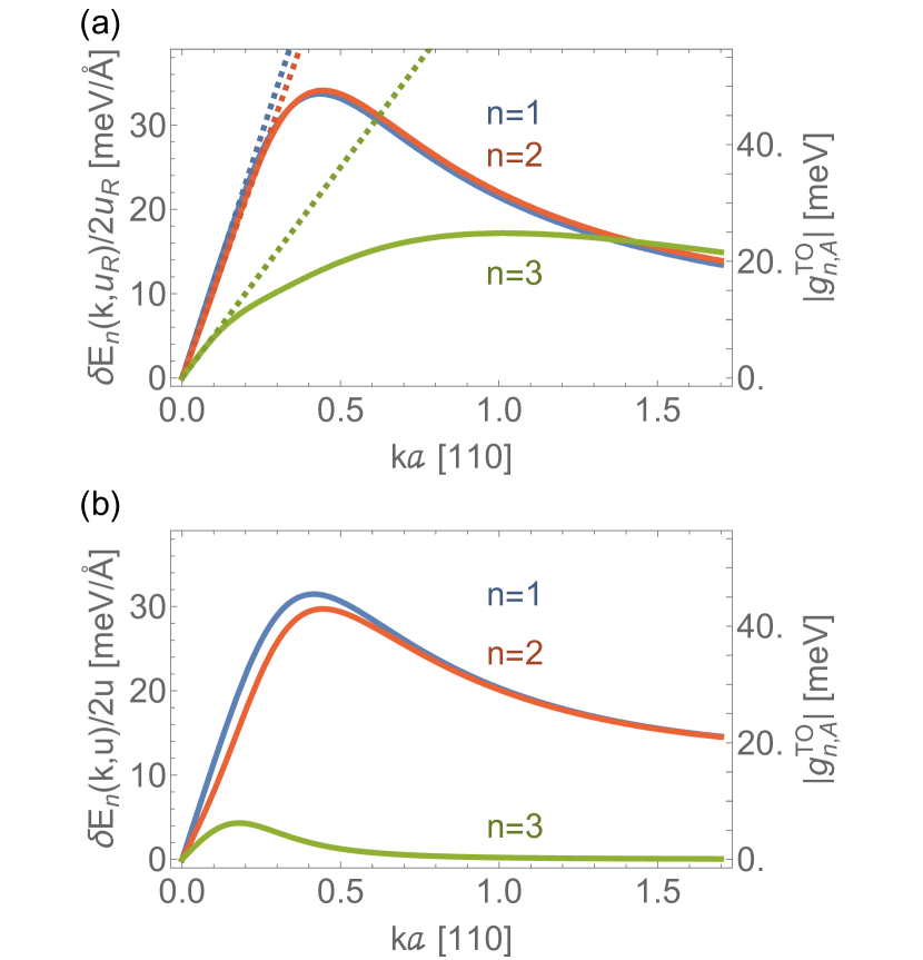
Figure 6: Electronic band split for the three bands of STO in the presence of a frozen polar mode with eigenvector deduced from Raman [Eq. (37)] and with polar axis $\bm{\hat{n}}_{p}^{E_{u}}\parallel[1\bar{1}0]$ and momentum $\bm{k}\parallel[110]$. The right $y$-axis shows the corresponding generalized Rashba electron-phonon matrix element [Eq. (40)]. Solid lines in (a) are ab initio results and dashed lines the conventional Rashba model [Eq. (25) and Eq. (34)]. Panel (b) is the result for minimal $t_{2g}$ model in Eqs. (13), (27) and (41) with the coupling matrix element corresponding to the Raman determined eigenvector, $2\partial_{x}t_{xy0}=\tau^{\mathcal{R}}_{1,A}=115$ meV/Å (extracted from DFT results in (a)).

Figure 6(a) shows the ab initio results (solid lines) of the pseudospin-split of each $n$ band going beyond the small $ka$ values presented in Fig. 3. We chose a frozen-phonon $E_{u}$ Raman mode [Eq. (37)] with polar axis $\hat{\bm{n}}_{p}\parallel[1\bar{1}0]$, and show the band split along the perpendicular momentum direction $\hat{\bm{k}}\parallel[110]$. As seen, for all bands the band-split $\delta E_{n}$ is initially conventional Rashba-like (growing linearly with momenta), but deviates from linearity and peaks at intermediate values of momenta after which steadily decreases in a form close to $1/k$.

To linear-in-$k$ order the splittings are given by the Rashba couplings through Eq. (25) and Eq. (34). We can generalize Eq. (34) to an arbitrary odd function of $k$ by introducing for each electronic band $n$,

$$g^{\bm{q}\alpha}_{n,l}=ka\mathcal{F}_{n,l}(ka)\sqrt{\frac{\hbar}{2m_{u}\omega_{\bm{q}\alpha}}}\tau^{(\alpha)}_{n,l},$$ (40)

were we defined $\mathcal{F}_{n,l}(ka)$ such that it is even in $k$ and $\mathcal{F}_{n,l}(ka)\rightarrow 1$ for $k\rightarrow 0$. By definition, the electron-phonon matrix element is proportional to the band split so $\mathcal{F}_{n,l}(ka)$ was extracted directly from the ab initio results. The corresponding $g_{n,A}^{\mathrm{TO}}$ is given by the right $y$-axis in Fig. 6(a). We anticipate that this dome in $k$ results in a dome in electronic density for both $\lambda_{\mathrm{BCS}}$ and $T_{c}$ so it is important to discuss its origin, which we do next.

VI.2 Minimal model and dome behavior

The dome-like behavior of the band split can be traced back to a $k$-dependent quenching of angular momentum. The essential physics is captured by the minimal model in Eq. (1) supplemented by a one-parameter simplification of the polar interaction in Eq. (27). Namely we keep only the spin-conserving $j=0$ term and restrict to mixing of $x$ and $y$ orbitals,

$$t_{xy0}(\bm{k},\bm{q})=2i\partial_{x}t_{xy0}u(\bm{q})\left[-\sin\left(k_{y}a\right)\hat{n}_{px}+\sin\left(k_{x}a\right)\hat{n}_{py}\right]$$ (41)

Computing the band splitting along $\hat{\bm{k}}\parallel[110]$ for $\hat{\bm{n}}_{p}\parallel[1\bar{1}0]$ one obtains panel (b) of Fig. 6. As seen, this simple approximation captures very well the coupling of the first two bands including the dome behavior. It underestimates the coupling of the third band which therefore calls for additional parameters beyond the scope of this subsection.

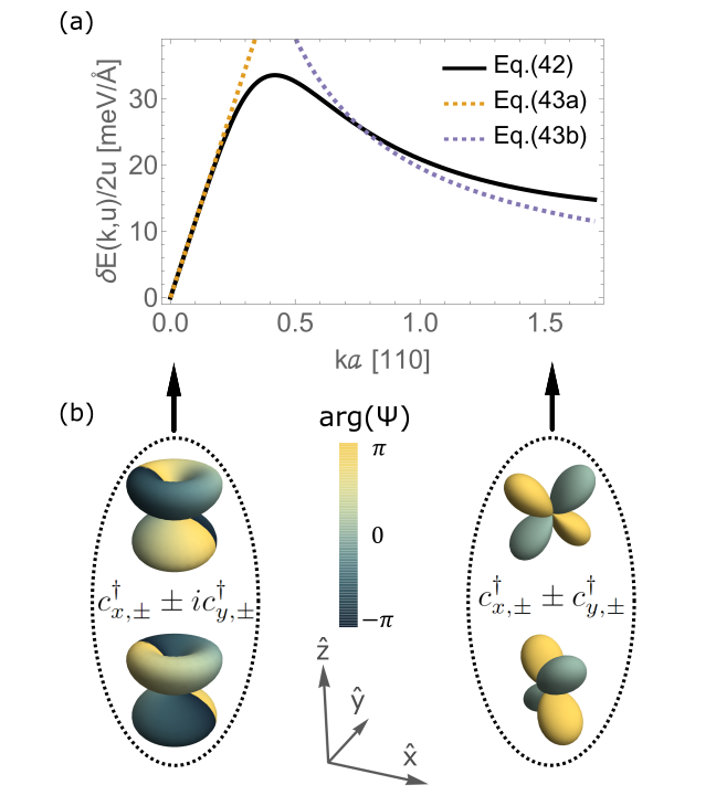
Figure 7: (a) Band split for two-orbital toy-model Eq. (42), and the perturbative limits Eqs. (43a)-(43b). (b) $k$-dependence of eigenstates, in the perturbative limits shown in (a). The color legend represents the argument of the wave function.

Focusing on the lowest band, the wave function near $\Gamma$ [Eq. (7)], suggests to simplify even more the tight-binding $t_{2g}$ model Eq. (1) by restricting it to two orbitals $\mu=x,y$, which is formally equivalent to taking the AFD parameter to infinity, $\Delta\rightarrow\infty$ in Eq. (4). The band split $\delta E$ of this toy-model for a finite $u(\bm{q})$ and the same $\hat{\bm{k}}$ and $\hat{\bm{n}}_{p}$ orientations as above can be analytically obtained from the eigenvalues of a $2\times 2$ matrix with matrix elements,

$$h_{11} =h_{22}=2\left(t_{1}+t_{2}+2t_{3}\right)\left[1-\cos\left(\frac{ka}{\sqrt{2}}\right)\right]$$

$$h_{12} =h_{21}^{*}=i\xi-4t_{4}\sin^{2}\left(\frac{ka}{\sqrt{2}}\right)+2i\partial_{x}t_{xy0}u\sqrt{2}\sin\left(\frac{ka}{\sqrt{2}}\right)$$

and reads

$$\frac{\delta E(k[110],u[1\bar{1}0])}{2u}=\frac{\tau_{1,A}\sqrt{2}\sin\left(\frac{ka}{\sqrt{2}}\right)}{\sqrt{1+\left[\frac{4t_{4}\sin^{2}\left(\frac{ka}{\sqrt{2}}\right)}{\xi}\right]^{2}}},$$ (42)

where we have used the relation $2\partial_{x}t_{xy0}=\tau_{1,A}$ [ Eq. (30)]. Expanding to linear order in $k$ one recovers the conventional Rashba form of Ref. [30] which here is generalized to arbitrary momentum.

Equation (42) is plotted in Fig. 7(a) for the electronic parameters in STO $t_{4}$ and $\xi$ listed in Sec. II.2, and $\tau^{\mathcal{R}}_{1,A}=115$ meV/Å corresponding to the Raman deduced soft-mode eigenvector. As seen, the two-orbital toy model excellently captures the band split of the lowest band, $n=1$, computed by DFT [c.f. Fig. 6(a) and Fig. 7(a)]. Furthermore, the analytical result for $n=2$ is identical to the $n=1$ case while in DFT both are very similar. Thus, surprisingly, the two-orbital toy-model provides a good approximation to the second band despite its non-negligible weight of the $z$-orbital near $\Gamma$ [Eq. (8)]. This is attributed to the rapid decrease of the $z$-orbital character as momentum increases along $[110]$. Indeed, including the $z$ orbital results in little change on the splittings for $n=1,2$ [Fig. 6(b)].

The $k$-dependence in Eq. (42) is determined by the competition between the SOC energy $\xi$ in $\mathcal{H}_{\mathrm{SOC}}$ (which dominates at $k=0$), and the hopping term $4t_{4}\sin^{2}\left(\frac{ka}{\sqrt{2}}\right)$ [Eq. (6)] which induces a mass mismatch of the bands in $\mathcal{H}_{0}$, and increases with $k$. The former term promotes a state with $l_{z}=\pm 1$ angular momentum $c^{\dagger}_{x,\pm}\pm ic^{\dagger}_{y,\pm}$ [Eq. (7)] leading to $j_{z}=\pm 3/2$ states, whereas the latter term constrains the system towards $c^{\dagger}_{x,\pm}\pm c^{\dagger}_{y,\pm}$ states which have $\langle{\bm{l}}\rangle=0$. This $k$-dependent quenching of angular momentum is illustrated in Fig. 7(b) where the complex, $l_{z}=\pm 1$ (real, $\langle\bm{l}\rangle=0$) orbitals for small (large) $k$ are shown.

Doing perturbation in Eq.(42) in the two opposite limits, where the SOC term dominates over the hopping term and vice versa, one obtains the following expressions for the band split in the continuum limit ($ka\ll 1$),

$$\frac{\delta E}{2u}\approx \tau_{1,A}ka\left[1+\mathcal{O}\left(\frac{t_{4}^{2}(ka)^{4}}{\xi^{2}}\right)\right],\ \ \ \ t_{4}(ka)^{2}\ll\xi$$ (43a)

$$\frac{\delta E}{2u}\approx \frac{\tau_{1,A}\xi}{2t_{4}ka}\left[1+\mathcal{O}\left(\frac{\xi^{2}}{t_{4}^{2}(ka)^{4}}\right)\right],\ \ \ \ \xi\ll t_{4}(ka)^{2}$$ (43b)

We recover the Rashba linear-in-$k$ term Eq. (25) when the SOC energy term dominates over the hopping term [Eq. (43a)], and the $1/k$ dependence in the opposite limit, when the kinetic term takes over [Eq. (43b)]. These two perturbative expressions are shown in Fig. 7(a) together with the full expression Eq. (42), by dashed orange and purple lines, respectively. Deviations of the expansion at large momentum are due to lattice effects which were neglected as they do not change the qualitative picture. Clearly, when the angular momentum becomes quenched the spin-orbit assisted electron-phonon interaction becomes ineffective and dies out. In the continuum limit the maximum of the coupling is given by

$$k^{max}a=\sqrt{\frac{\xi}{2t_{4}}}\approx 0.42,$$ (44)

which again illustrates the competition between spin orbit and band mass mismatch energies. The right hand side corresponds to the present parameters, relevant for STO. As it will be clear below, the maximum of the coupling is the more important factor to determine the optimum Fermi momentum and density for superconductivity.

Because the pairing interaction arising from the polar coupling is in turn proportional to the square of the electron-phonon matrix element [30] (shown in the right $y$-axis of Fig. 6), $V_{\mathrm{TO}}\propto|g^{\mathrm{TO}}|^{2}$, it also acquires a pronounced peak as a function of $k=k_{F}$, the Fermi momentum. The initial quadratic increase with $k_{F}$ peaks and decreases as $V_{\mathrm{TO}}\propto 1/k_{F}^{2}$ for all three bands. Consequently the pairing coupling constant[30] $\lambda_{\mathrm{BCS},A}=\frac{2}{3}N_{F}V_{\mathrm{TO}}\propto k_{F}V_{\mathrm{TO}}$ of each band (assuming parabolic bands) shows a dome-like form with increasing $k_{F}$ [inset of Fig. 8]. We took a constant factor of 2 effective mass enhancement in $N_{F}$, chosen to match the values from specific heat [83] at low carrier densities. This mass renormalization can be viewed as effectively taking into account the coupling to other phonons not considered explicitly so far, such as the longitudinal optical modes.

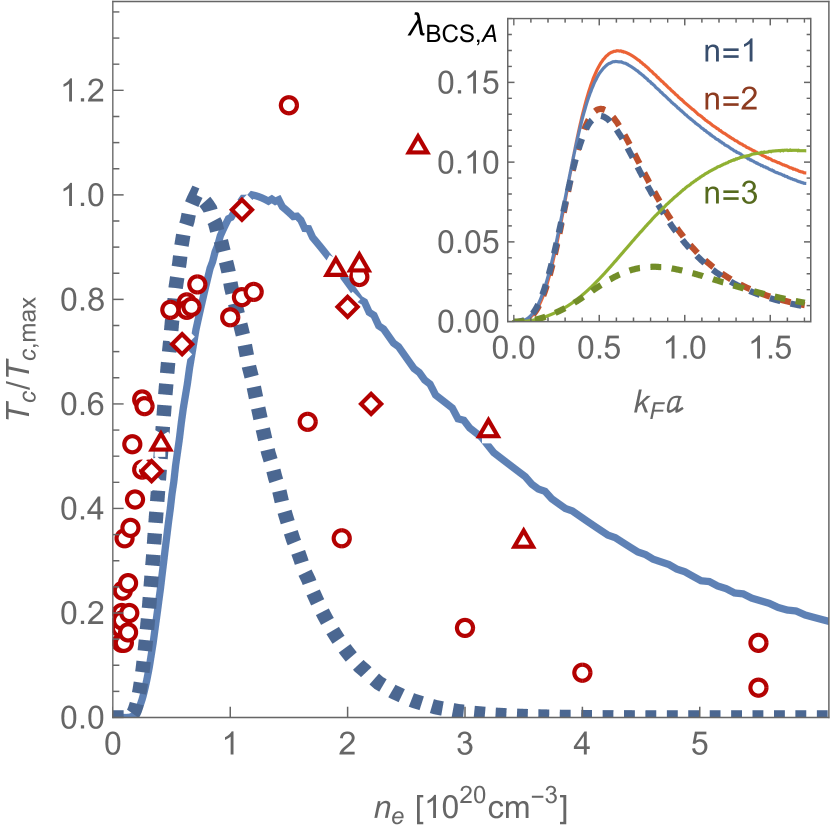
Figure 8: $T_{c}$ dome (normalized to its maximum value) vs. carrier density $n_{e}=\frac{k_{F}^{3}}{3\pi^{2}}$ assuming a parabolic band and using $\lambda_{\mathrm{BCS},A}$ from lowest band $n=1$ shown in inset. Full (dashed) line neglects (includes) the hardening of the TO mode. Inset: band resolved $\lambda_{\mathrm{BCS},A}=\frac{2}{3}N_{F}\frac{|g_{n,A}^{\mathrm{TO}}|^{2}}{\omega_{\mathrm{TO}}}$ using the ab initio results $g_{n,A}^{\mathrm{TO}}$ of Fig. 6(a). Open symbols are bulk $T_{c}$ experimental data from Ref. [84] (circles), Ref. [85](triangles) and Ref. [86] (diamonds) with $T_{c,max}=0.35$K. Notice that for simplicity an effective one-band is considered in the theory to compute $n_{e}$, while in the experiment $n_{e}$ is the total electronic density.

The obtained values of $\lambda_{\mathrm{BCS},A}$ are in the weak coupling limit so we can use a simple BCS formalism. This is in agreement with the $2\Delta(T=0)/T_{c}$ ratio obtained with tunneling and microwave spectroscopy studies [86, 87] which suggest that a weak coupling picture applies. Neglecting inter-band (finite-$q$) couplings in Eq. (22), we obtain three uncoupled SC gap equations, one for each electronic band. In this approximation, the higher $T_{c}$ corresponds to the bulk critical temperature of the material.

This simplified picture already predicts a dome of $T_{c}\propto\exp[-1/\lambda_{BCS,A}]$ within the generalized Rashba coupling pairing mechanism, shown in Fig. 8 for the first band $n=1$. Notice that the largest $T_{c}$ corresponds to $n=2$, but since both curves are very similar there is little difference on which one is chosen. Note also that we are assuming a rigid band picture, which seems to be a good approximation for bulk SC obtained by Nb and La doping [88].

Within the present mechanism, we believe that the dominant correction to the above computation of the dome is given by the hardening of the TO mode with carrier density [17, 31], $\tilde{\omega}_{\mathrm{TO}}(k_{F}a)=\sqrt{\omega_{\mathrm{TO}}^{2}+D(k_{F}a)^{3}}$ with $D=1.64\mathrm{meV}^{2}$. This parametrization was chosen to match the factor of three hardening of the soft mode at low temperatures when reaching $n_{e}=1.5\times 10^{20}$ as measured by infra-red spectroscopy[89]. As seen by the dashed lines in Fig. 8, since $\lambda_{\mathrm{BCS}}\propto 1/\omega^{2}_{\mathrm{TO}}$, the hardening reduces the pairing constant even faster at high Fermi momenta where the hardening effect is largest. Consequently, the $T_{c}$ dome is narrowed and shifted to lower densities.

VI.3 Comparison with experiments

A key prediction of the present mechanism is the density where $T_{c}$ peaks, which including (neglecting) the hardening of the soft mode is found to be $n^{opt}_{e}\approx 7\times 10^{19}$ cm^-3 ($n^{opt}_{e}\approx 1\times 10^{20}$ cm^-3 ). This can slightly change by multiband effects and mass anisotropy but the order of magnitude is in excellent agreement with diamagnetic experiments[90, 84, 86], without free parameters. To the best of our knowledge, the fine resolution in carrier density achieved in early Refs. [90, 84] has not since been attained in bulk superconductivity measurements. To determine the experimental optimum density, we have neglected two outlier points in Ref. [84] that were neglected also in their fit and a similar outlier point in the data of Ref. [85], which unfortunately does not cover the maxima of Refs. [90, 84, 86]. More experimental and theoretical work is needed to understand if those outliers are a systematic effect. Eventually, they may be attributed to multiband effects neglected here. Furthermore, we are not taking into consideration resistivity data, as it is not a bulk superconductivity probe. Indeed, $T_{c}$ in bulk probes (specific heat, thermal conductivity and diamagnetism) is consistently lower than the zero-resistance $T$, which points towards filamentary superconductivity at higher temperatures and extremely dilute samples [2, 91, 88].

When plotted in linear scale, it becomes clear that the dome is very asymmetric, with a rapid rise and a much slower decrease [Fig. 8]. Also, this asymmetry is well reproduced by the theory presented here. The rise of $T_{c}$ appears at a density slightly higher than in experiments while the decrease is very sensitive to what is assumed for the hardening of the soft mode. Within the present uncertainties on the experimental data [Fig. 8], also the width and the asymmetry of the dome are in very good agreement with experiment.

An important remaining question is if the present theory can explain the observed maximum value of $T_{c}$. In Ref. [30] we used the naive $k$-linear Rashba form, neglected the phonon hardening, and obtained a good estimate of $T_{c}$ near optimum density. The present computations show that both approximations can lead to an overestimation of $\lambda_{\mathrm{BCS}}$. On the other hand, a pure Slater mode $\bar{S}_{1}$ was assumed; Eq. (39) shows that the details of the soft mode eigenvector strongly affects the coupling strength. For the soft mode eigenvector found by hyper-Raman [Eq. (37)], the overestimation error of Ref. [30] tends to cancel with the amplification of Eq. (39) so the computed $\lambda_{\mathrm{BCS}}$ is again close to the one required by experiments. Indeed, taking the BCS form $k_{B}T_{c}=1.13\hbar\omega_{TO}\exp[-1/\lambda_{\mathrm{BCS}}]$ and assuming the soft mode frequency to be $\omega_{TO}=3$ meV near the optimum density requires a $\lambda_{\mathrm{BCS}}=0.21$ to obtain a maximum transition temperature near the experimental one[90, 84, 86, 2] ($T_{c,max}\approx 0.35$ K). In our computation the maximum $\lambda_{\mathrm{BCS}}$, including phonon hardening, is $\lambda_{max}=0.13$ [see inset of Fig. 8] which is fairly close to this BCS estimate without any free parameters. Thus, it is clear that the present mechanism can explain the observed $T_{c}$ as $\lambda_{max}$ is in the correct range.

As explained above, our estimate of $\lambda_{\mathrm{BCS}}$ is a lower bound. A more accurate computation should take into account that around optimum carrier density, three bands are filled; our estimate takes into account only one band. Also, the contributions of $g_{n,B}$ and $g_{n,C}$ matrix elements to the $A_{1g}$ pairing channel have been neglected. Both of these aspects are expected to increase $T_{c}$ and hence improve the agreement with the experiment. While one can incorporate the above corrections in the computations, in practice, due to the exponential dependence of $T_{c}$ with $\lambda_{\mathrm{BCS}}$ and the approximate treatment of the Coulomb interaction [92] (neglected in this work), a high level of accuracy in $T_{c}$ should not to be expected. Therefore, for the time being, we consider the present results robust enough to claim that the magnitude of $T_{c}$ can be explained within the present mechanism. As mentioned earlier, the coupling of electrons to pairs of TO modes, that is, the quadratic coupling to the FE mode, is also a promising source of pairing in doped paraelectrics, and certainly in doped STO [33, 34, 35, 36, 37]. Also, for this mechanism, a dome-like feature of $T_{c}$ vs. doping and an optimum density in good agreement with experiment has been found without free parameters [36]. Therefore, more experimental and theoretical work is needed to decide which of the two mechanisms is more appropriate to describe the superconducting dome.

We remark that the dome arising in Ref. [36] is due to the hardening of the phonons with electronic carrier density, with the quadratic coupling constant in the interaction vertex left as a constant. In the work presented here, on the other hand, the momentum dependence (odd-parity) of the linear coupling constant already gives rise to a dome (see full lines in Fig. 8), and the hardening of the soft phonon modifies its shape (dashed lines in Fig. 8).

Charge transport in the normal state of doped STO presents a pronounced $T^{2}$ regime in the resistivity present even at very low $n_{e}$ where umklapp scattering is forbidden. This behavior has been explained invoking the combination of scattering by a LO mode and two-TO modes [42] as well as a LO mode and a single-TO mode over a range of temperatures [31]. This suggests both linear and quadratic coupling mechanisms are consistent with the observed $T^{2}$ resistivity. Whether the momentum structure of the linear coupling found in this work can discriminate between the two scenarios for charge transport is left for a future study.

VII Summary and Conclusions

In this work, we have derived the most general Rashba-like linear coupling between the electronic bands and the polar modes at the zone center of tetragonal STO [Eq. (IV.1)]. Fitting the electronic band split of the Rashba model [Eqs. (25)-(26)] to ab initio $q=0$ frozen-phonon calculations [Fig. 3] we have estimated the corresponding Rashba couplings, $\tau^{(\bar{S}_{i})}_{n,l}$, to zone center polar modes $\bar{S}_{i}$ [Fig. 4(a)]. These $\bar{S}_{i}$ modes form a complete basis of in-plane, $E_{u}$, and out-of-plane, $A_{2u}$, modes at the zone center in STO [Eqs. (15)-(19)] and hence we have mapped out the entire Rashba-like linear coupling subspace of these zone-center polar modes.

The origin of the Rashba couplings can be understood as arising from induced hopping channels between neighboring $t_{2g}$ orbitals in the presence of polar distortions [Eqs. (27)]. We have explicitly shown how to connect the symmetry allowed Rashba-coupling constants $\tau_{n,l}$ in Eq. (IV.1) to the microscopic hopping processes $\partial_{l}t_{\mu\nu}$ [Eqs. (29) and (30)]. Indeed, a minimal, three-orbital model with only one induced hopping parameter reproduces qualitatively and to some extent quantitatively many results of the ab initio computations [Fig. (6)].

We have shown how to estimate the electron-polar-phonon coupling function of a general polar mode by decomposing it into the $\bar{S}_{i}$ basis [Eqs. (V)-(V)] using the obtained Rashba-couplings $\tau^{(\bar{S}_{i})}_{n,l}$ [Fig. 4(a)]. Since an accurate determination of the soft-mode eigenvector is difficult, this allows us to separate the problem of determining the coupling to the soft mode from the problem of determining its eigenvector.

Starting from eigenvector cases of a Slater mode $\bar{S}_{1}$ and those consistent with neutron data [Eq. (36)] and hyper-Raman data [Eq. (37)] in STO, we have obtained and compared three sets of electron-TO-phonon couplings $g_{n,l}^{\mathrm{TO}}$ [Fig. 4(b) and Table 2]. We find substantial coupling values for the three electronic bands, with the $E_{u}$ coupling $g_{n,A}^{\mathrm{TO}}$ being larger than the other two couplings $g_{n,B}^{\mathrm{TO}}$ and $g_{n,C}^{\mathrm{TO}}$. Physically, the $A$ component of the $E_{u}$ irrep corresponds to the case in which the pseudospin lies along the $z$-direction, as considered in Ref. [30] and in the toy-model of Sec. VI.2.

We found that the details of the eigenvector can substantially alter the magnitude of the couplings. In particular, the intermediate contribution of the $\bar{S}_{3}$ mode (which distorts the oxygen octahedra) to the Raman determined eigenvector [Eq. (37)] significantly increases the $E_{u}$ coupling $g_{n,A}^{\mathrm{TO}}$ for all three bands [see Fig. 4(b)].

Certainly, the sensitivity of the couplings to the eigenvector has important implications for the Rashba pairing mechanism [30], since the BCS coupling constant $\lambda_{BCS}$ is proportional to the square of the electron-TO-phonon coupling in its simplest form. Comparison with the DFT broken symmetry state suggests that the oxygen cage should deform substantially in the soft mode as found by the hyper-Raman eigenvector. More experimental and theoretical work will be highly desirable to refine the eigenvector of the soft mode and improve the estimate of $\lambda_{\mathrm{BCS}}$.

While the linear-in-$k$ conventional Rashba model works well at low momenta, our ab initio frozen phonon results generally indicate a deviation from the linear-$k$ Rashba split of the three electronic bands beyond a critical wave vector for all polar modes. As a result, we find a dome-like behavior of the electron-TO-phonon coupling $g_{n,l}^{\mathrm{TO}}$ [Eq. (40)]: beyond the critical wave vector the linear-$k$ growth slows and peaks, subsequently evolving into a $1/k$ decrease [Fig. 6]. This behavior is due to a $k$-dependent quenching of the angular momentum, as explicitly shown by reducing the three-orbital model to a two-orbital toy model [Eq. (42) and Fig. 7].

Assuming a rigid band shift for electronic doping, and without introducing electronic screening effects, this deviation from Rashba already entails a dome for $T_{c}$ as a function of electronic density. We remark that this result does not depend crucially on the particular form of the polar mode eigenvector. A popular explanation of the dome invokes the proximity to a ferroelectric quantum critical point [1]. In the simplest picture, the dome is attributed to the change of the frequency of the soft-mode with density, possibly with the structural transition laying below the dome [93]. This last simplified picture, however, requires that the system breaks inversion symmetry to the right or to the left of the optimum density which, to the best of our knowledge, is not the case. In the mechanism we presented, the proximity to the ferroelectric quantum critical point is important to have a soft-mode in the first place, which increases $\lambda_{\mathrm{BCS}}\propto 1/\omega_{\mathrm{TO}}^{2}$, but it is not responsible for the non-monotonous behavior of $T_{c}$. Including the hardening with doping increases the agreement with the experimental data of Refs. [84, 90] [Fig. 8].

The obtained maximum value of $T_{c}$, the density at which it peaks, and the characteristic asymmetry of the dome are in surprisingly good agreement with experiments without free parameters [Fig. 8] providing a compelling solution to a more than 50 year old open problem in the field. Small deviations remain, which we attribute to several simplifications we have made to avoid introducing more parameters in the theory. For example, additional Rashba coupling contributions to the $A_{1g}$ pairing channel can be considered, which will increase $T_{c}$ and possibly decrease the smaller density at which bulk superconductivity becomes robust. It remains an interesting question for future research to find out if the spin-orbit processes neglected [labeled $B$ and $C$ in Eq. (IV.1)] can stabilize different pairing symmetries other than the conventional $s$-wave we have considered.

The approach presented here can be generalized to study the linear coupling characteristics between electrons and FE soft TO modes, as well as the corresponding pairing mechanism in other incipient ferroelectrics. A noteworthy example are KTO interfaces, where the linear coupling to the TO mode has recently been invoked for pairing [51].

References

- Edge et al. [2015] J. M. Edge, Y. Kedem, U. Aschauer, N. A. Spaldin, and A. V. Balatsky, Quantum Critical Origin of the Superconducting Dome in SrTiO3, Phys. Rev. Lett. 115, 247002 (2015).
- Collignon et al. [2019] C. Collignon, X. Lin, C. W. Rischau, B. Fauqué, and K. Behnia, Metallicity and Superconductivity in Doped Strontium Titanate, Annual Review of Condensed Matter Physics 10, 25 (2019).
- Herrera et al. [2019] C. Herrera, J. Cerbin, A. Jayakody, K. Dunnett, A. V. Balatsky, and I. Sochnikov, Strain-engineered interaction of quantum polar and superconducting phases, Phys. Rev. Materials 3, 124801 (2019).
- Ahadi et al. [2019] K. Ahadi, L. Galletti, Y. Li, S. Salmani-Rezaie, W. Wu, and S. Stemmer, Enhancing superconductivity in films with strain, Science Advances 5, eaaw0120 (2019).
- Salmani-Rezaie et al. [2021a] S. Salmani-Rezaie, H. Jeong, R. Russell, J. W. Harter, and S. Stemmer, Role of locally polar regions in the superconductivity of , Phys. Rev. Materials 5, 104801 (2021a).
- Salmani-Rezaie et al. [2021b] S. Salmani-Rezaie, H. Jeong, K. Ahadi, and S. Stemmer, Interplay between Polar Distortions and Superconductivity in SrTiO3, Microscopy and Microanalysis 27, 360–362 (2021b).
- Hameed et al. [2022] S. Hameed, D. Pelc, Z. W. Anderson, A. Klein, R. Spieker, L. Yue, B. Das, J. Ramberger, M. Lukas, Y. Liu, et al., Enhanced superconductivity and ferroelectric quantum criticality in plastically deformed Strontium Titanate, Nature Materials 21, 54 (2022).
- Stucky et al. [2016] A. Stucky, G. Scheerer, Z. Ren, D. Jaccard, J.-M. Poumirol, C. Barreteau, E. Giannini, and D. van der Marel, Isotope effect in superconducting n-doped SrTiO3, Scientific reports 6, 37582 (2016).
- Rischau et al. [2017] C. W. Rischau, X. Lin, C. P. Grams, D. Finck, S. Harms, J. Engelmayer, T. Lorenz, Y. Gallais, B. Fauque, J. Hemberger, et al., A ferroelectric quantum phase transition inside the superconducting dome of Sr1-xCaxTiO3-δ, Nature Physics 13, 643 (2017).
- Tomioka et al. [2019] Y. Tomioka, N. Shirakawa, K. Shibuya, and I. H. Inoue, Enhanced superconductivity close to a non-magnetic quantum critical point in electron-doped Strontium Titanate, Nature Communications 10, 738 (2019).
- Tomioka et al. [2022] Y. Tomioka, N. Shirakawa, and I. H. Inoue, Superconductivity enhancement in polar metal regions of Sr0.95Ba0.05TiO3 and Sr0.985Ca0.015TiO3 revealed by systematic Nb doping, npj Quantum Materials 7, 111 (2022).
- Rischau et al. [2022] C. W. Rischau, D. Pulmannová, G. W. Scheerer, A. Stucky, E. Giannini, and D. van der Marel, Isotope tuning of the superconducting dome of strontium titanate, Phys. Rev. Research 4, 013019 (2022).
- Schumann et al. [2020] T. Schumann, L. Galletti, H. Jeong, K. Ahadi, W. M. Strickland, S. Salmani-Rezaie, and S. Stemmer, Possible signatures of mixed-parity superconductivity in doped polar films, Phys. Rev. B 101, 100503 (2020).
- Yerzhakov et al. [2022] H. Yerzhakov, R. Ilan, E. Shimshoni, and J. Ruhman, Majorana-weyl cones in ferroelectric superconductors, arXiv preprint arXiv:2205.08563 (2022).
- Kanasugi et al. [2020] S. Kanasugi, D. Kuzmanovski, A. V. Balatsky, and Y. Yanase, Ferroelectricity-induced multiorbital odd-frequency superconductivity in , Phys. Rev. B 102, 184506 (2020).
- Franklin et al. [2021] J. Franklin, B. Xu, D. Davino, A. Mahabir, A. V. Balatsky, U. Aschauer, and I. Sochnikov, Giant grüneisen parameter in a superconducting quantum paraelectric, Phys. Rev. B 103, 214511 (2021).
- Gastiasoro et al. [2020a] M. N. Gastiasoro, J. Ruhman, and R. M. Fernandes, Superconductivity in dilute SrTiO3: A review, Annals of Physics 417, 168107 (2020a).
- Takada [1980] Y. Takada, Theory of superconductivity in polar semiconductors and its application to n-type semiconducting srtio3, Journal of the Physical Society of Japan 49, 1267 (1980).
- Ruhman and Lee [2016] J. Ruhman and P. A. Lee, Superconductivity at very low density: The case of strontium titanate, Phys. Rev. B 94, 224515 (2016).
- Wölfle and Balatsky [2019] P. Wölfle and A. V. Balatsky, Reply to “Comment on ‘Superconductivity at low density near a ferroelectric quantum critical point: Doped ”’, Phys. Rev. B 100, 226502 (2019).
- Enderlein et al. [2020] C. Enderlein, J. F. de Oliveira, D. Tompsett, E. B. Saitovitch, S. Saxena, G. Lonzarich, and S. Rowley, Superconductivity mediated by polar modes in ferroelectric metals, Nature communications 11, 1 (2020).
- Edelman and Littlewood [2021] A. Edelman and P. B. Littlewood, Normal state correlates of plasmon-polaron superconductivity in strontium titanate, arXiv preprint arXiv:2111.03138 (2021).
- Lin et al. [2021] L. Lin, P. B. Littlewood, and A. Edelman, Analysis of fröhlich bipolarons, arXiv preprint arXiv:2111.12250 (2021).
- Arce-Gamboa and Guzmán-Verri [2018] J. R. Arce-Gamboa and G. G. Guzmán-Verri, Quantum ferroelectric instabilities in superconducting , Phys. Rev. Materials 2, 104804 (2018).
- Kedem [2018] Y. Kedem, Novel pairing mechanism for superconductivity at a vanishing level of doping driven by critical ferroelectric modes, Phys. Rev. B 98, 220505 (2018).
- Kozii et al. [2019] V. Kozii, Z. Bi, and J. Ruhman, Superconductivity near a ferroelectric quantum critical point in ultralow-density dirac materials, Phys. Rev. X 9, 031046 (2019).
- Gastiasoro et al. [2020b] M. N. Gastiasoro, T. V. Trevisan, and R. M. Fernandes, Anisotropic superconductivity mediated by ferroelectric fluctuations in cubic systems with spin-orbit coupling, Phys. Rev. B 101, 174501 (2020b).
- Sumita and Yanase [2020] S. Sumita and Y. Yanase, Superconductivity induced by fluctuations of momentum-based multipoles, Phys. Rev. Research 2, 033225 (2020).
- Yoon et al. [2021] H. Yoon, A. G. Swartz, S. P. Harvey, H. Inoue, Y. Hikita, Y. Yu, S. B. Chung, S. Raghu, and H. Y. Hwang, Low-density superconductivity in srtio3 bounded by the adiabatic criterion, arXiv preprint arXiv:2106.10802 (2021).
- Gastiasoro et al. [2022] M. N. Gastiasoro, M. E. Temperini, P. Barone, and J. Lorenzana, Theory of superconductivity mediated by Rashba coupling in incipient ferroelectrics, Phys. Rev. B 105, 224503 (2022).
- Yu et al. [2022] Y. Yu, H. Y. Hwang, S. Raghu, and S. B. Chung, Theory of superconductivity in doped quantum paraelectrics, npj Quantum Materials 7, 1 (2022).
- Kozii et al. [2021] V. Kozii, A. Klein, R. M. Fernandes, and J. Ruhman, Synergetic ferroelectricity and superconductivity in zero-density dirac semimetals near quantum criticality, arXiv preprint arXiv:2110.09530 (2021).
- Ngai [1974] K. L. Ngai, Two-phonon deformation potential and superconductivity in degenerate semiconductors, Phys. Rev. Lett. 32, 215 (1974).
- van der Marel et al. [2019] D. van der Marel, F. Barantani, and C. W. Rischau, Possible mechanism for superconductivity in doped , Phys. Rev. Research 1, 013003 (2019).
- Kiselov and Feigel’man [2021] D. E. Kiselov and M. V. Feigel’man, Theory of superconductivity due to Ngai’s mechanism in lightly doped , Phys. Rev. B 104, L220506 (2021).
- Volkov et al. [2022] P. A. Volkov, P. Chandra, and P. Coleman, Superconductivity from energy fluctuations in dilute quantum critical polar metals, Nature communications 13, 1 (2022).
- Zyuzin and Zyuzin [2022] V. A. Zyuzin and A. A. Zyuzin, Anisotropic resistivity and superconducting instability in ferroelectric metals, Phys. Rev. B 106, L121114 (2022).
- Volkov and Chandra [2020] P. A. Volkov and P. Chandra, Multiband quantum criticality of polar metals, Phys. Rev. Lett. 124, 237601 (2020).
- Kumar et al. [2022] A. Kumar, P. Chandra, and P. A. Volkov, Spin-phonon resonances in nearly polar metals with spin-orbit coupling, Phys. Rev. B 105, 125142 (2022).
- Klein et al. [2022] A. Klein, V. Kozii, J. Ruhman, and R. M. Fernandes, A theory of criticality for quantum ferroelectric metals, arXiv preprint arXiv:2209.02733 (2022).
- Ruhman and Lee [2019] J. Ruhman and P. A. Lee, Comment on “superconductivity at low density near a ferroelectric quantum critical point: Doped ”, Phys. Rev. B 100, 226501 (2019).
- Kumar et al. [2021] A. Kumar, V. I. Yudson, and D. L. Maslov, Quasiparticle and nonquasiparticle transport in doped quantum paraelectrics, Phys. Rev. Lett. 126, 076601 (2021).
- Fu [2015] L. Fu, Parity-breaking phases of spin-orbit-coupled metals with gyrotropic, ferroelectric, and multipolar orders, Phys. Rev. Lett. 115, 026401 (2015).
- Kozii and Fu [2015] V. Kozii and L. Fu, Odd-parity superconductivity in the vicinity of inversion symmetry breaking in spin-orbit-coupled systems, Phys. Rev. Lett. 115, 207002 (2015).
- Wu and Martin [2017] F. Wu and I. Martin, Nematic and chiral superconductivity induced by odd-parity fluctuations, Phys. Rev. B 96, 144504 (2017).
- Kanasugi and Yanase [2019] S. Kanasugi and Y. Yanase, Multiorbital ferroelectric superconductivity in doped , Phys. Rev. B 100, 094504 (2019).
- Petersen and Hedegård [2000] L. Petersen and P. Hedegård, A simple tight-binding model of spin–orbit splitting of sp-derived surface states, Surface Science 459, 49 (2000).
- Liu et al. [2021] C. Liu, X. Yan, D. Jin, Y. Ma, H.-W. Hsiao, Y. Lin, T. M. Bretz-Sullivan, X. Zhou, J. Pearson, B. Fisher, et al., Two-dimensional superconductivity and anisotropic transport at ktao3 (111) interfaces, Science 371, 716 (2021).
- Chen et al. [2021] Z. Chen, Y. Liu, H. Zhang, Z. Liu, H. Tian, Y. Sun, M. Zhang, Y. Zhou, J. Sun, and Y. Xie, Electric field control of superconductivity at the laalo3/ktao3 (111) interface, Science 372, 721 (2021).
- Mallik et al. [2022] S. Mallik, G. Ménard, G. Saïz, H. Witt, J. Lesueur, A. Gloter, L. Benfatto, M. Bibes, and N. Bergeal, Superfluid stiffness of a ktao3-based two-dimensional electron gas, Nature Communications 13, 1 (2022).
- Liu et al. [2022] C. Liu, X. Zhou, D. Hong, B. Fisher, H. Zheng, J. Pearson, D. Jin, M. R. Norman, and A. Bhattacharya, Tunable superconductivity at the oxide-insulator ktao3 interface and its origin, arXiv preprint arXiv:2203.05867 (2022).
- Kresse and Furthmüller [1996] G. Kresse and J. Furthmüller, Efficient iterative schemes for ab initio total-energy calculations using a plane-wave basis set, Physical review B 54, 11169 (1996).
- Kresse and Joubert [1999] G. Kresse and D. Joubert, From ultrasoft pseudopotentials to the projector augmented-wave method, Physical review b 59, 1758 (1999).
- Perdew et al. [2008] J. P. Perdew, A. Ruzsinszky, G. I. Csonka, O. A. Vydrov, G. E. Scuseria, L. A. Constantin, X. Zhou, and K. Burke, Restoring the density-gradient expansion for exchange in solids and surfaces, Physical review letters 100, 136406 (2008).
- Steiner et al. [2016] S. Steiner, S. Khmelevskyi, M. Marsmann, and G. Kresse, Calculation of the magnetic anisotropy with projected-augmented-wave methodology and the case study of disordered alloys, Phys. Rev. B 93, 224425 (2016).
- Bistritzer et al. [2011] R. Bistritzer, G. Khalsa, and A. H. MacDonald, Electronic structure of doped perovskite semiconductors, Phys. Rev. B 83, 115114 (2011).
- van der Marel et al. [2011] D. van der Marel, J. L. M. van Mechelen, and I. I. Mazin, Common Fermi-liquid origin of resistivity and superconductivity in -type SrTiO3, Phys. Rev. B 84, 205111 (2011).
- Zhong et al. [2013] Z. Zhong, A. Tóth, and K. Held, Theory of spin-orbit coupling at LaAlO3/SrTiO3 interfaces and SrTiO3 surfaces, Phys. Rev. B 87, 161102 (2013).
- sug [1970] Chapter vii - spin-orbit interaction, in Multiplets of Transition-Metal Ions in Crystals, Pure and Applied Physics, Vol. 33, edited by S. Sugano, Y. Tanabe, and H. Kamimura (Elsevier, 1970) pp. 154–178.
- Khomskii and Streltsov [2020] D. I. Khomskii and S. V. Streltsov, Orbital effects in solids: basics, recent progress, and opportunities, Chemical Reviews 121, 2992 (2020).
- Stamokostas and Fiete [2018] G. L. Stamokostas and G. A. Fiete, Mixing of orbitals in and transition metal oxides, Phys. Rev. B 97, 085150 (2018).
- [62] See supplemental material at [url] for details on computation, soc eigenstates and rashba coupling results.
- Axe [1967] J. D. Axe, Apparent ionic charges and vibrational eigenmodes of bati and other perovskites, Phys. Rev. 157, 429 (1967).
- Harada et al. [1970] J. Harada, J. Axe, and G. Shirane, Determination of the normal vibrational displacements in several perovskites by inelastic neutron scattering, Acta Crystallographica Section A: Crystal Physics, Diffraction, Theoretical and General Crystallography 26, 608 (1970).
- Vogt [1988] H. Vogt, Hyper-Raman tensors of the zone-center optical phonons in and , Phys. Rev. B 38, 5699 (1988).
- Cowley [1964] R. A. Cowley, Lattice dynamics and phase transitions of strontium titanate, Phys. Rev. 134, A981 (1964).
- Slater and Koster [1954] J. C. Slater and G. F. Koster, Simplified lcao method for the periodic potential problem, Phys. Rev. 94, 1498 (1954).
- Yamanaka et al. [2000] A. Yamanaka, M. Kataoka, Y. Inaba, K. Inoue, B. Hehlen, and E. Courtens, Evidence for competing orderings in Strontium Titanate from hyper-Raman scattering spectroscopy, EPL (Europhysics Letters) 50, 688 (2000).
- Russell et al. [2019] R. Russell, N. Ratcliff, K. Ahadi, L. Dong, S. Stemmer, and J. W. Harter, Ferroelectric enhancement of superconductivity in compressively strained films, Phys. Rev. Materials 3, 091401 (2019).
- Salmani-Rezaie et al. [2020a] S. Salmani-Rezaie, K. Ahadi, W. M. Strickland, and S. Stemmer, Order-Disorder Ferroelectric Transition of Strained , Phys. Rev. Lett. 125, 087601 (2020a).
- Salmani-Rezaie et al. [2020b] S. Salmani-Rezaie, K. Ahadi, and S. Stemmer, Polar nanodomains in a ferroelectric superconductor, Nano Letters 20, 6542 (2020b).
- Shigenari [2015] T. Shigenari, Raman spectra of soft modes in ferroelectric crystals, in Ferroelectric Materials, edited by A. P. Barranco (IntechOpen, Rijeka, 2015) Chap. 1.
- Bednorz and Müller [1984] J. G. Bednorz and K. A. Müller, : An quantum ferroelectric with transition to randomness, Phys. Rev. Lett. 52, 2289 (1984).
- Nova et al. [2019] T. Nova, A. Disa, M. Fechner, and A. Cavalleri, Metastable ferroelectricity in optically strained SrTiO3, Science 364, 1075 (2019).
- [75] H. T. Stokes, D. M. Hatch, and B. J. Campbell, Isodistort, isotropy software suite, iso.byu.edu.
- Campbell et al. [2006] B. J. Campbell, H. T. Stokes, D. E. Tanner, and D. M. Hatch, ISODISPLACE: a web-based tool for exploring structural distortions, Journal of Applied Crystallography 39, 607 (2006).
- Khalsa et al. [2013] G. Khalsa, B. Lee, and A. H. MacDonald, Theory of electron-gas rashba interactions, Phys. Rev. B 88, 041302 (2013).
- Djani et al. [2019] H. Djani, A. C. Garcia-Castro, W.-Y. Tong, P. Barone, E. Bousquet, S. Picozzi, and P. Ghosez, Rationalizing and engineering rashba spin-splitting in ferroelectric oxides, npj Quantum Materials 4, 1 (2019).
- Zhou et al. [2018] J.-J. Zhou, O. Hellman, and M. Bernardi, Electron-phonon scattering in the presence of soft modes and electron mobility in perovskite from first principles, Phys. Rev. Lett. 121, 226603 (2018).
- He et al. [2020] X. He, D. Bansal, B. Winn, S. Chi, L. Boatner, and O. Delaire, Anharmonic eigenvectors and acoustic phonon disappearance in quantum paraelectric , Phys. Rev. Lett. 124, 145901 (2020).
- Shin et al. [2021] D. Shin, S. Latini, C. Schäfer, S. A. Sato, U. De Giovannini, H. Hübener, and A. Rubio, Quantum paraelectric phase of from first principles, Phys. Rev. B 104, L060103 (2021).
- Fauqué et al. [2022a] B. Fauqué, P. Bourges, A. Subedi, K. Behnia, B. Baptiste, B. Roessli, T. Fennell, S. Raymond, and P. Steffens, Mesoscopic tunneling in strontium titanate, arXiv preprint arXiv:2203.15495 (2022a).
- McCalla et al. [2019] E. McCalla, M. N. Gastiasoro, G. Cassuto, R. M. Fernandes, and C. Leighton, Low-temperature specific heat of doped : Doping dependence of the effective mass and kadowaki-woods scaling violation, Phys. Rev. Materials 3, 022001 (2019).
- Koonce et al. [1967] C. S. Koonce, M. L. Cohen, J. F. Schooley, W. R. Hosler, and E. R. Pfeiffer, Superconducting Transition Temperatures of Semiconducting SrTiO3, Phys. Rev. 163, 380 (1967).
- Collignon et al. [2017] C. Collignon, B. Fauqué, A. Cavanna, U. Gennser, D. Mailly, and K. Behnia, Superfluid density and carrier concentration across a superconducting dome: The case of strontium titanate, Phys. Rev. B 96, 224506 (2017).
- Thiemann et al. [2018] M. Thiemann, M. H. Beutel, M. Dressel, N. R. Lee-Hone, D. M. Broun, E. Fillis-Tsirakis, H. Boschker, J. Mannhart, and M. Scheffler, Single-gap superconductivity and dome of superfluid density in nb-doped , Phys. Rev. Lett. 120, 237002 (2018).
- Swartz et al. [2018] A. G. Swartz, H. Inoue, T. A. Merz, Y. Hikita, S. Raghu, T. P. Devereaux, S. Johnston, and H. Y. Hwang, Polaronic behavior in a weak-coupling superconductor, Proceedings of the National Academy of Sciences 115, 1475 (2018).
- Fauqué et al. [2022b] B. Fauqué, C. Collignon, H. Yoon, X. Lin, H. Y. Hwang, K. Behnia, et al., An electronic band sculpted by oxygen vacancies and indispensable for dilute superconductivity, arXiv preprint arXiv:2208.09831 (2022b).
- Devreese et al. [2010] J. T. Devreese, S. N. Klimin, J. L. M. Van Mechelen, and D. Van Der Marel, Many-body large polaron optical conductivity in SrTi1-xNbxO3, Phys. Rev. B 81, 125119 (2010).
- Schooley et al. [1965] J. F. Schooley, W. R. Hosler, E. Ambler, J. H. Becker, M. L. Cohen, and C. S. Koonce, Dependence of the superconducting transition temperature on carrier concentration in Semiconducting SrTiO3, Phys. Rev. Lett. 14, 305 (1965).
- Bretz-Sullivan et al. [2019] T. M. Bretz-Sullivan, A. Edelman, J. Jiang, A. Suslov, D. Graf, J. Zhang, G. Wang, C. Chang, J. E. Pearson, A. B. Martinson, et al., Superconductivity in the dilute single band limit in reduced Strontium Titanate, arXiv preprint arXiv:1904.03121 (2019).
- Marsiglio [2022] F. Marsiglio, Impact of retardation in the holstein-hubbard model: a two-site calculation, arXiv preprint arXiv:2205.10352 (2022).
- Setty et al. [2022] C. Setty, M. Baggioli, and A. Zaccone, Superconducting dome in ferroelectric-type materials from soft mode instability, Phys. Rev. B 105, L020506 (2022).