On RKHS Choices for Assessing Graph Generators via Kernel Stein Statistics

Abstract

Score-based kernelised Stein discrepancy (KSD) tests have emerged as a powerful tool for the goodness of fit tests, especially in high dimensions; however, the test performance may depend on the choice of kernels in an underlying reproducing kernel Hilbert space (RKHS). Here we assess the effect of RKHS choice for KSD tests of random networks models, developed for exponential random graph models (ERGMs) in Xu and Reinert, (2021) and for synthetic graph generators in Xu and Reinert, (2022). We investigate the power performance and the computational runtime of the test in different scenarios, including both dense and sparse graph regimes. Experimental results on kernel performance for model assessment tasks are shown and discussed on synthetic and real-world network applications.

1 Introduction

Recent advances in high-dimensional goodness of fit tests have been achieved by score-based kernelised Stein discrepancy (KSD) tests, starting with Chwialkowski et al., (2016) and Liu et al., (2016). A KSD test relies on an underlying reproducing kernel Hilbert space (RKHS) and hence its performance may depend on the choice of RKHS for the set of test functions. Typically, the choice of RKHS is restricted by having to lie in the Stein class of the target distribution (see Section 2 for details). A notable exception is the case that the target distribution is that of a finite random network, as then any finite function is a member of the Stein class. Thus, this situation is well suited to assessing the choice of RKHS.

In this paper we assess the choice of RKHS for the two available graph-based kernelised Stein goodness of fit tests, which take a single network as input, namely gKSS from Xu and Reinert, (2021) and AgraSSt from Xu and Reinert, (2022). The RKHS kernels which we explore are the constant kernel, the vertex-edge histogram kernel (Kriege et al.,, 2016), the shortest path kernel (Borgwardt and Kriegel,, 2005), random walk kernels (Gärtner et al.,, 2003; Sugiyama and Borgwardt,, 2015), the Weisfeiler-Lehman kernel (Shervashidze et al.,, 2011), the graphlet kernel (Ahmed et al.,, 2017) and the connected graphlet kernel (Shervashidze et al.,, 2009). As the influence of the RKHS choice on the power of the goodness of fit test may depend on the problem setting, here we investigate a collection of test problems, including edge-two star (E2S) models, geometric random graph (GRG) models, Barabasi-Albert (BA) models, and the black-box random graph generator CELL (Rendsburg et al.,, 2020). The kernel choice may also have a significant effect on the runtime which is hence included in the analysis.

The paper is structured as follows. In Section 2, we introduce the basic form of kernel Stein statistics and its corresponding goodness-of-fit testing procedure.Then we discuss kernel choices in Section 3. In Section 4, we present the experimental results on E2S models relating to the experiments in Xu and Reinert, (2021), the GRG models, as well as in CELL, trained on real-world networks, followed by concluding discussions. Additional background, results on the BA models and a GRG on a unit square, as well as a computational efficient algorithm for geometric random walk kernels are deferred to the appendix. Code for the experiment is available at https://github.com/MoritzWeckbecker/dissertation-kss.

2 Background: kernel Stein statistic for random graph models

Let $\mathcal{G}_{n}^{lab}$ denote the set of vertex-labeled simple graphs on $n$ vertices. For a probability distribution $q$, an operator $\mathcal{T}_{q}$ on $\mathcal{G}_{n}^{lab}$ satisfying the Stein identity $\mathbb{E}_{q}[\mathcal{T}_{q}f(x)]=0$ for all test functions $f:\mathcal{G}_{n}^{lab}\to\mathbb{R}$ in a Stein class $\mathcal{F}$ is called a Stein operator. With $q(x^{(s,1)}|{x_{-s}})$ denoting the conditional probability that vertex pair $s$ has an edge, given the network except the edge indicator of $s$ (and similarly $q(x^{(s,0)}|{x_{-s}})$ the conditional probability that vertex pair $s$ does not have an edge) so that $q(x^{(s,\cdot)}|{x_{-s}})$ is a discrete score function, the Stein operator in Xu and Reinert, (2021) is $\mathcal{T}_{q}f=\frac{1}{N}\sum_{s\in[N]}\mathcal{T}^{(s)}_{q}f$ where

$${\mathcal{T}_{q}^{(s)}f(x)}=q(x^{(s,1)}|{x_{-s}})f(x^{(s,1)})+q(x^{(s,0)}|{x_{-s}})f(x^{(s,0)})-f(x).$$

If a distribution $p$ is close to $q$ then one would expect that $\mathbb{E}_{p}[\mathcal{T}_{q}f(x)]\approx 0$; hence $\sup_{f\in{\mathcal{F}}}|\mathbb{E}_{p}[\mathcal{T}_{q}f(x)]|$ can be used to assess the distributional distance between $q$ and $p$. Choosing as ${\mathcal{F}}$ the unit ball of a RKHS $\mathcal{H}$ allows to compute the supremum exactly. The kernel Stein statistic (KSS) based on a single network sample $x$ is defined as

$$\operatorname{KSS}(q;x)=\sup_{\|f\|_{\mathcal{H}}\leq 1}\left|\mathbb{E}_{q(\cdot|x)}[f(X_{t_{1}})|X_{0}=x]-f(x)\right|=\sup_{\|f\|_{\mathcal{H}}\leq 1}\Big{|}\frac{1}{N}\sum_{s\in[N]}\left[\mathcal{T}^{(s)}_{q}f(x)\right]\Big{|}.$$ (1)

For computational efficiency, instead of averaging over all $N$ possible edges, a vertex pair re-sampling version is also provided. Let the re-sample size be $B$, then draw $\{s_{1},\dots,s_{B}\}$ uniformly from $[N]$. Denote $k$ the kernel associate with $\mathcal{H}$. Then we estimate

$$\widehat{\operatorname{KSS}}^{2}(q;x)=\sup_{\|f\|_{\mathcal{H}}\leq 1}\Big{|}\frac{1}{B}\sum_{b\in[B]}\left[\mathcal{T}^{(s_{b})}_{q}f(x)\right]\Big{|}^{2}=\frac{1}{B^{2}}\sum_{b,b^{\prime}}\underset{{h(s_{b},s_{b^{\prime}})}}{\underbrace{\left\langle\mathcal{T}^{(s_{b})}_{q}k(x,\cdot),\mathcal{T}^{(s_{b^{\prime}})}_{q}k(x,\cdot)\right\rangle}},$$

where $h$ is referred to as the Stein kernel. When $q$ is the distribution of an exponential random graph model, KSS coincides with gKSS from Xu and Reinert, (2021). When $q$ does not have an explicit form, e.g. for samples from $q$ generated by a black-box random graph generator, Xu and Reinert, (2022) approximate the conditional distribution using samples generated from $q$ to estimate the conditional score function.

Xu and Reinert, (2022) also suggest conditioning on a user-defined graph summary statistic $t(x)$ and replacing $q(x^{(s,1)}|x_{-s})$ by $\widehat{q}(x^{(s,1)}|t(x_{-s}))$ in Eq.(1) ; this is termed the approximate graph Stein Statistic (AgraSSt) in Xu and Reinert, (2022). In Xu and Reinert, (2021) and Xu and Reinert, (2022) theoretical guarantees are also given.

For testing the goodness of fit of the model $q$ based on a single network observation $x$, gKSS and AgraSSt use the Monte Carlo procedure, simulating $l$ independent networks $z_{1},\dots,z_{l}\sim q$ and comparing the observed $\widehat{\operatorname{KSS}}^{2}(q;x)$ with the set of $\widehat{\operatorname{KSS}}^{2}(q;z_{i}),{i=1\in[l]}$. We reject the null model if $\widehat{\operatorname{KSS}}(q;x)$ is large. Details are given in Algorithm 1 in Appendix A.

3 Graph kernel choices and their effects on KSS

Graph kernels considered

While details of the Gaussian vertex-edge histogram (GVEH) kernel, the shortest path (SP) kernel, the $K$-step random walk (KRW) and geometric random walk (GRW) kernels, and the Weisfeiler-Lehman (WL) kernels can be found in Appendix B of (Xu and Reinert,, 2021), we recollect them in Section A.3. We additionally consider graphlet counts (sub-graphs with a small number of vertices), as the features to compare graph structures.

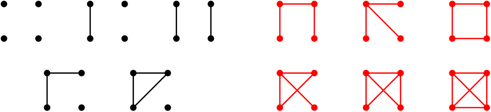
Figure 1: Graphlets illustration for $l=4$: $N_{4}=11$; the connected graphlets are marked as red.

The idea of a graphlet kernel (Ahmed et al.,, 2017) is to count the occurrences of all simple undirected graphs of size $l$, up to permutation of the vertices, $\{\mathfrak{g}_{1},\dots,\mathfrak{g}_{N_{l}}\}$ where $N_{l}$ denotes the number of distinct $l$-graphlets. An example for $l=4$ is shown in Figure 1. The graphlet feature $\phi_{glet}(x)\in\mathbb{N}^{N_{l}}$ has as $i$-th entry the number of occurrences of $\mathfrak{g}_{i}$ in $x$. This feature naturally induces the graphlet kernel $k_{GLET}(x,x^{\prime})=\langle\phi_{glet}(x),\phi_{glet}(x^{\prime})\rangle.$ When only the connected graphlets (e.g. Figure 1 in red) are considered to construct the feature $\phi_{conglet}(x)$, the connected graphlet kernel is given by $k_{CONGLET}(x,x^{\prime})=\langle\phi_{conglet}(x),\phi_{conglet}(x^{\prime})\rangle.$

Graph kernels	Parameters
GVEH	bandwidth $\sigma>0$
KRW	maximal walk length $K$
GRW	discount weight $\lambda$
WL	level parameter $h$
GLET	size of graphlets $l$

Table 1: Graph kernels and the parameters.

For our experiment, we use the implementation provided by the R package graphkernels (Sugiyama et al.,, 2018). In addition, we devise the “constant” kernel $k_{Const}(x,x^{\prime})\equiv 1$ as a benchmark in our experiment. Like the SP kernel, the constant kernel has no parameter.

We list the parameters for the kernels in Table 1.

4 Experimental results

In our experiments the observed network is assumed to be generated by model $M0$, and the goodness of fit is tested for model $M1$; the null hypothesis $H_{0}:M0=M1$ is rejected in favour of $H_{1}:M0\neq M1$ at the $5\%$-level using a gKSS or an AgraSSt test with $n_{M1}$ graphs simulated under $M1$. In the synthetic examples we repeat this procedure on $n_{M0}$ graphs from the null model to obtain the rejection rate. Unless otherwise stated, $n_{M0}=n_{M1}=500.$ More details can be found in Appendix B.

An ERGM example

The Edge-2Star (E2S) model on $\mathcal{G}_{n}^{lab}$ is an ERGM with density $q(x)\propto\exp(\beta_{1}E(x)+\beta_{s}S_{2}(x))$ where $E(x)$ denotes the edge count and $S_{2}$ denotes the number of two-stars. In our experiments, following the setting of Xu and Reinert, (2021) the null model is $\beta=(-2,0)$ and the alternative is set by perturbing $\beta_{2}$. As this is an ERGM, we apply an gKSS test (Xu and Reinert,, 2021); Figure 2 shows rejection rates for WL, GRW and graphlet kernels with different parameters. From the result, all kernels had well-controlled type 1 error, and even using a constant kernel already had good test power. While a WL kernel generally outperformed the constant kernel, GRW kernels of different parameters were outperformed by the constant kernel. This finding could perhaps be explained by the change in density between null and alternative; this change may already suffice for separating the two, and the constant kernel picks this up. In contrast, GRW kernels focus more on local structure. The graphlet kernels generally have similar test power compared to the constant kernel; they would pick up a change in density through a change in graphlet counts.

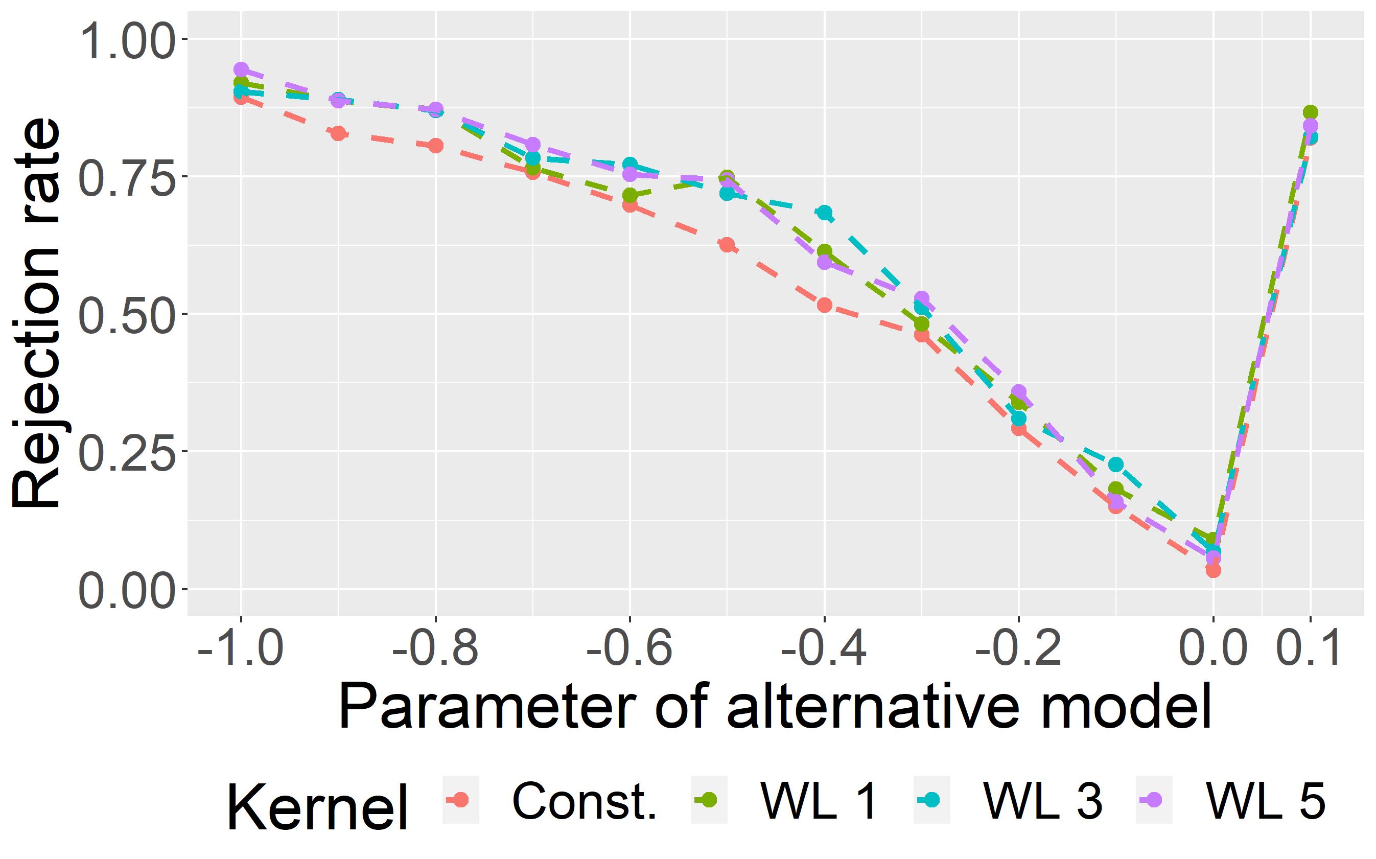
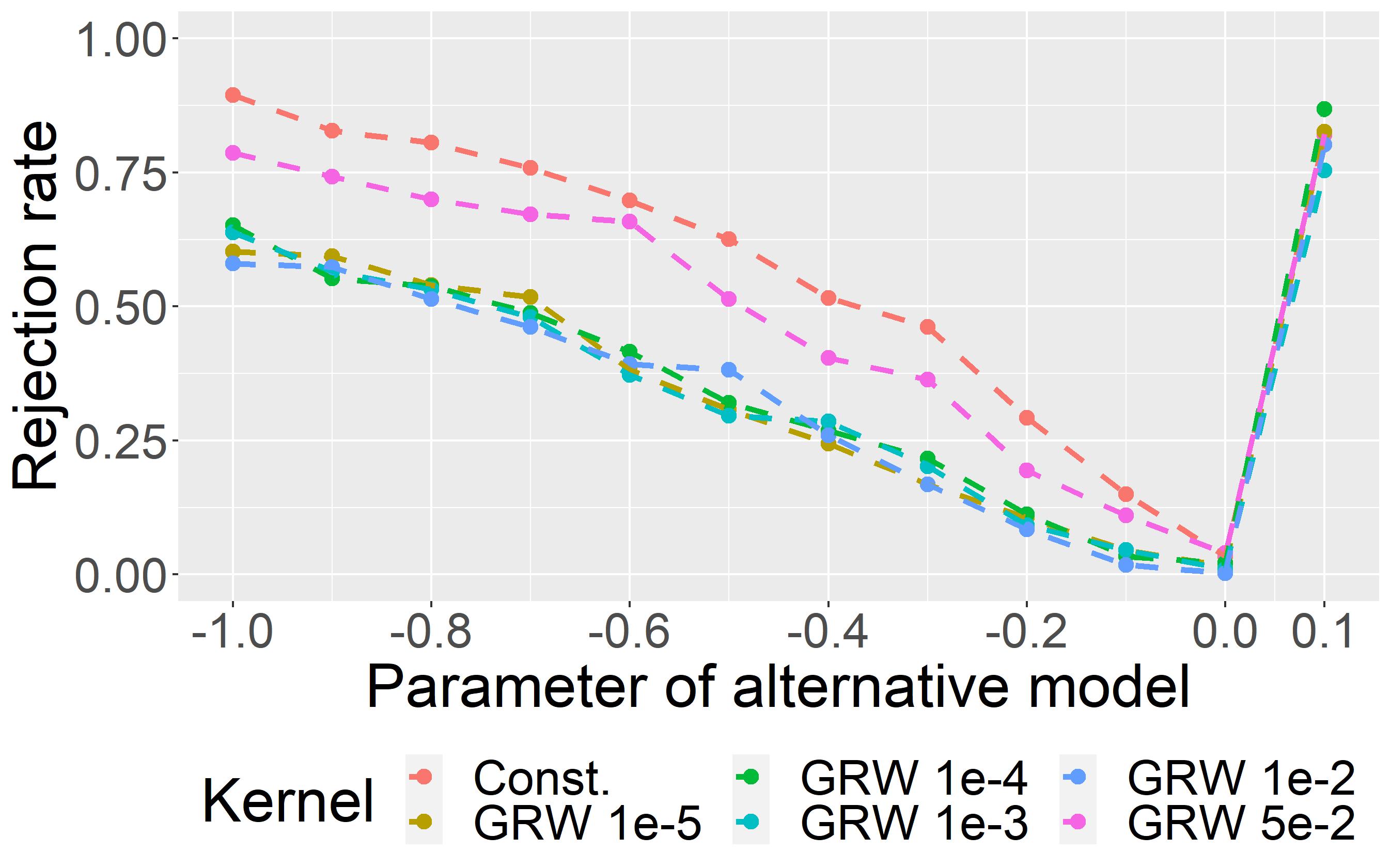
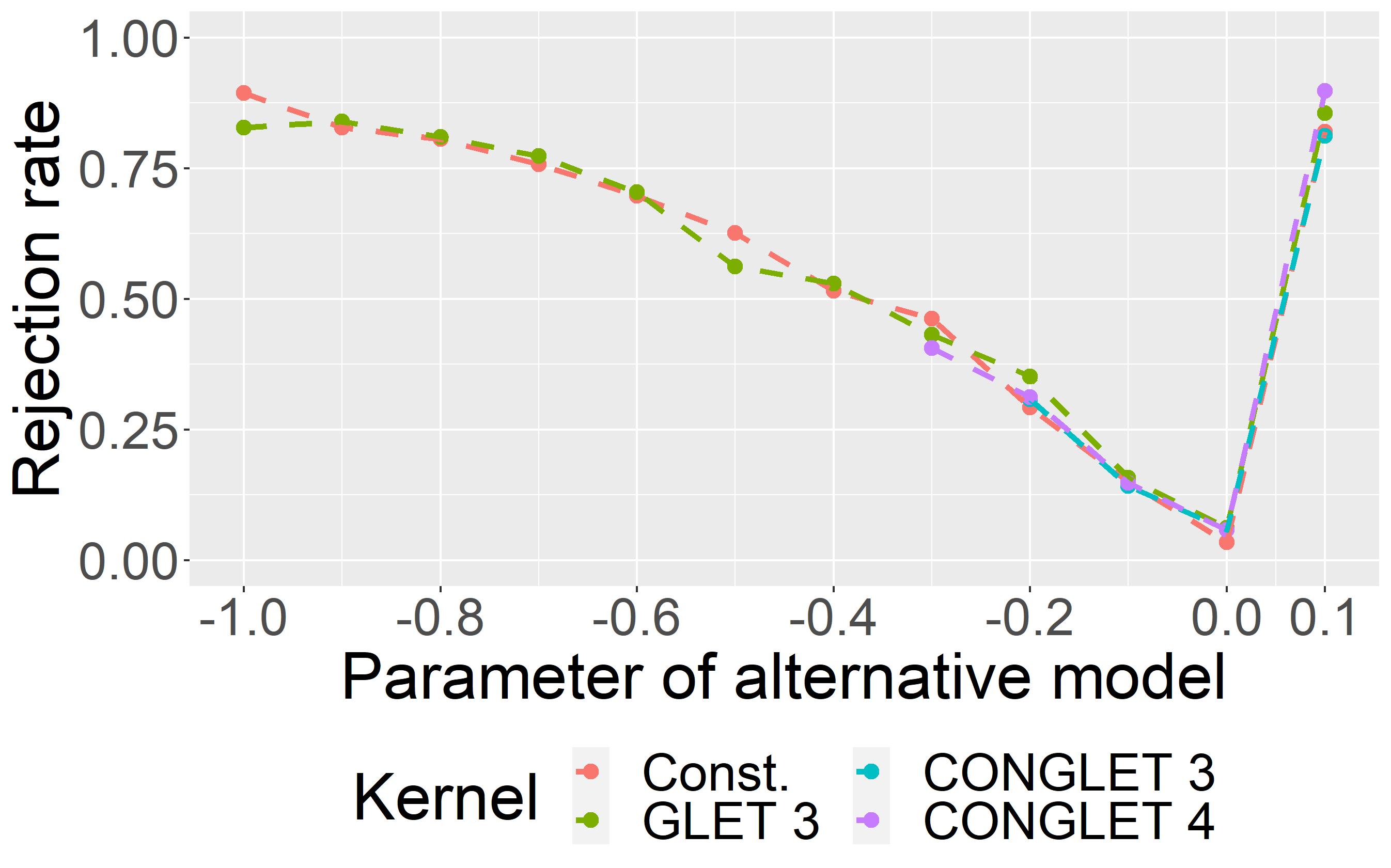
Figure 2: gKSS on the E2S model with $\beta_{2}$ perturbed; $n=20$ and $B=200$.

A geometric random graph example

In our geometric random graph (GRG) models (Penrose,, 2003), vertices are uniformly placed on a 2-dimensional unit torus and two vertices are connected by an edge if their distance is smaller than a pre-defined radius parameter $r$. The null model sets $r=0.3$ where the alternative is set by perturbing $r$. Here we use AgraSSt with some of the summary statistics suggested in Xu and Reinert, (2022). AgraSSt with a WL kernel as suggested in (Xu and Reinert,, 2022) achieves well controlled type 1 error in all presented settings in the main text and Appendix B. When using edge density as summary statistics, Figure 6 in Appendix B shows that all kernel choices achieve good performance, with the graphlet kernels performing best, and the constant kernel and GRW kernels performing better than the WL kernel. When using instead bi-degree as summary statistic for predicting conditional edge probability in AgraSSt (see Figure 3), there is a region around $r=0.45$ in which the test statistics struggle to distinguish the alternative from the null; an explanation can be found in Section B.1.4. Here, GVEH with small bandwidth exihibits the best performance. For GRG on a square instead of a torus, there is no such ambiguous region; results are shown in Appendix B.

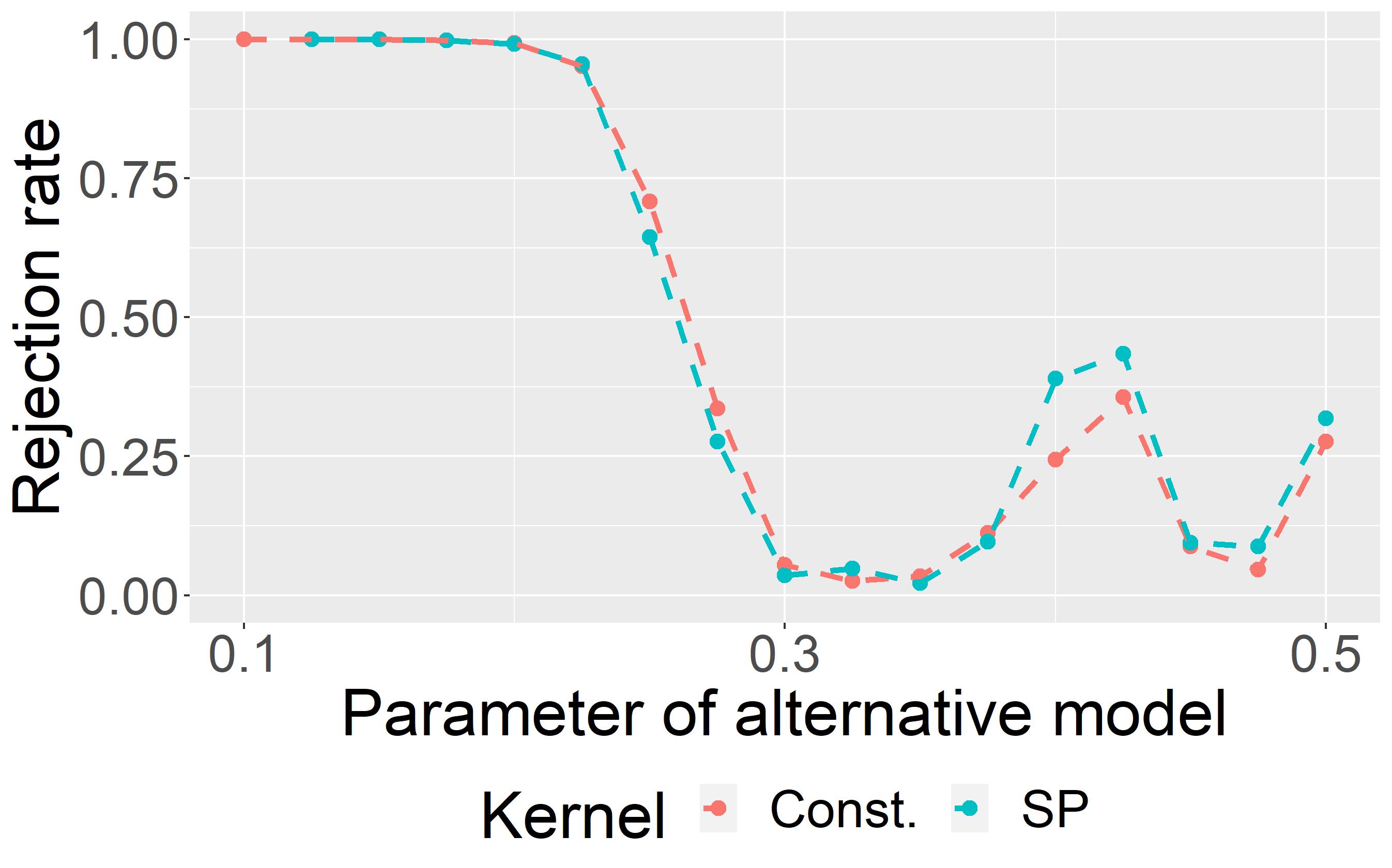
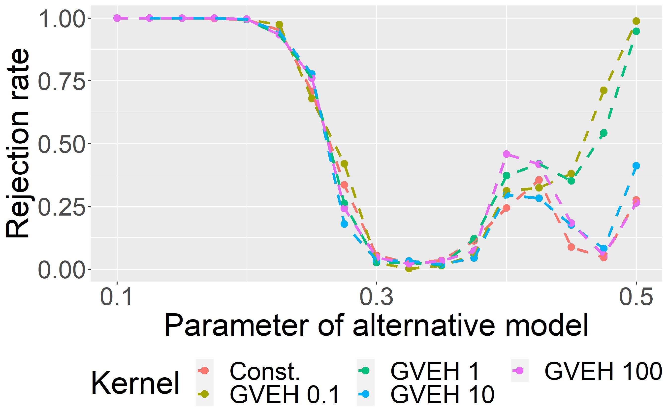
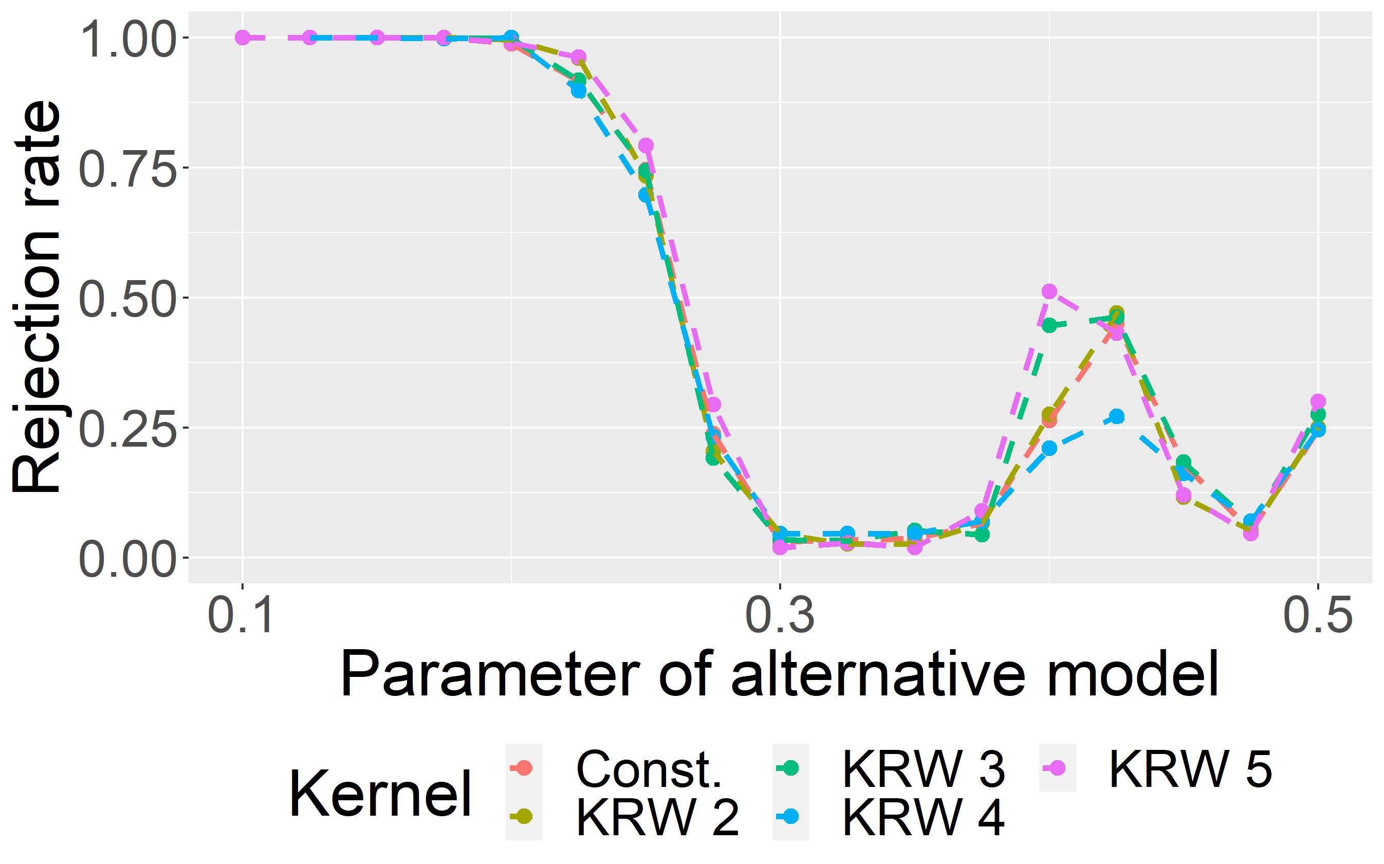
Figure 3: AgraSSt for the GRG model with perturbed $r$ alternatives; $n=20$ and $B=200$; $t(x)$ is set to be the bivariate (vertex) degree vector.

CELL

To assess the effect of kernel choice on a black-box deep generative model, we train the Cross-Entropy Low-rank Logit (CELL) (Rendsburg et al.,, 2020) on Zachary’s Karate Club network Zachary, (1977) using different kernels. Model $M1$ is obtained by training CELL on the Karate club network. Here we take $n_{M1}=100$; $n_{M0}=1$ as we observe only one network. We repeat the procedure 100 times to obtain average rejection rates. Rejection rates, shown in Table 5 in the Appendix, are reasonable for most kernels; GVEH struggles for some of the statistics, and so do KRW and GRW.

Runtimes

The runtimes of the algorithms, with their standard implementation from the R package graphkernels (Sugiyama et al.,, 2018), are shown in Table 6 and Table 7, for a sparse as well as a dense setting. The constant kernel is by far the fastest kernel, followed by WL kernels. The random walk and shortest path kernels take three to 6 orders of magnitude longer to compute than the constant kernel and their runtime is greatly increased by larger edge density. We note that the runtime depends on the implementation; Section C.2 includes an idea for speeding up GRW kernel computations.

5 Conclusion and Discussion

In this work, we explored the effect of kernel and parameter choices on KSS for model assessment. Beyond observing some case specific phenomena where some choices can outperform others, we also conclude that both gKSS and AgraSSt are fairly robust in producing decent test power under the alternative, using a large class of kernels. Overall the constant kernel, which does not encode network information beyond density, performs surprisingly well as soon as there is a distinguishing signal in the edge density. Given its clear runtime advantage if density is assumed to be a strong signal then this could be a reasonable kernel to use. Also it is reassuring that the WF kernels in AgraSSt perform well.

If runtime is not an issue, then one may like to combine tests based on suitably selected kernels as in Schrab et al., (2022), and reject the null hypothesis if any of the single kernel tests distinguishes the alternative from the null hypothesis by rejecting it.

In future work, it would be interesting to carry out a similar study for other KSD tests. In general then the additional issue of Stein class may feature, as not every kernel choice may yield a RKHS which is a Stein class for the operator.

Finally, Stein operators for distributions are not unique (Ley et al.,, 2017). Exploring the interplay between Stein operator choice and RKHS is another future research direction.

Appendix A Additional details on background

A.1 The graph kernel Stein statistic (gKSS)

The graph Kernel Stein statistic (gKSS) has been proposed to assess goodness of fit for the family of exponential random graph models (ERGMs). ERGMs are frequently used as parametric models for social network analysis (Wasserman and Faust,, 1994; Holland and Leinhardt,, 1981; Frank and Strauss,, 1986); they include Bernoulli random graphs as well as stochastic blockmodels as special cases. Here we restrict attention to undirected, unweighted simple graphs on $n$ vertices, without self-loops or multiple edges. To define such an ERGM, we introduce the following notations.

Let $\mathcal{G}^{lab}_{n}$ be a set of vertex-labeled graphs on $n$ vertices and, for $N=n(n-1)/2$, encode $x\in\mathcal{G}^{lab}_{n}$ by an ordered collection of $\{0,1\}$ valued variables $x=(x_{ij})_{1\leq i<j\leq n}\in\{0,1\}^{N}$ where $x_{ij}=1$ if and only if there is an edge between $i$ and $j$. For a graph $H$ on at most $n$ vertices, let $V(H)$ denote the vertex set, and for $x\in\{0,1\}^{N}$, denote by $t(H,x)$ the number of edge-preserving injections from $V(H)$ to $V(x)$; an injection $\sigma$ preserves edges if for all edges $vw$ of $H$ with $\sigma(v)<\sigma(w)$, $x_{\sigma(v)\sigma(w)}=1$. For $v_{H}=|V(H)|\geq 3$ set

$$t_{H}(x)=\frac{t(H,x)}{n(n-1)\cdots(n-v_{H}+3)}.$$

If $H{=H_{1}}$ is a single edge, then $t_{H}(x)$ is twice the number of edges of $x$. In the exponent this scaling of counts matches (Bhamidi et al.,, 2011, Definition 1) and (Chatterjee and Diaconis,, 2013, Sections 3 and 4). An ERGM for the collection $x\in\{0,1\}^{N}$ can be defined as follows, see Reinert and Ross, (2019).

Definition 1.

Fix $n\in\mathbb{N}$ and $c\in\mathbb{N}$. Let $H_{1}$ be a single edge and for $l={2},\ldots,c$ let $H_{l}$ be a connected graph on at most $n$ vertices; set $t_{l}(x)=t_{H_{l}}(x)$. For $\beta=(\beta_{1},\dots,\beta_{c})^{\top}{\in\mathbb{R}^{c}}$ and $t(x)=(t_{1}(x),\dots,t_{c}(x))^{\top}\in\mathbb{R}^{c}$ $X\in\mathcal{G}^{lab}_{n}$ follows the exponential random graph model $X\sim\operatorname{ERGM}(\beta,t)$ if for $\forall x\in\mathcal{G}^{lab}_{n}$,

$$\mathbb{P}(X=x)=\frac{1}{\kappa_{n}(\beta)}\exp{\left(\sum_{l=1}^{c}\beta_{l}t_{l}(x)\right)}.$$

Here $\kappa_{n}(\beta)$ is the normalisation constant.

The vector $\beta\in\mathbb{R}^{k}$ is the parameter vector and the statistics $t(x)=(t_{1}(x),\dots,t_{c}(x))^{\top}\in\mathbb{R}^{c}$ are sufficient statistics.

Many random graph models can be set in this framework. The simplest example is the Bernoulli random graph (ER graph) with edge probability $0<p<1$; in this case, $l=1$ and $H_{1}$ is a single edge. ERGMs can use other statistic in addition to subgraph counts, and many ERGMs model directed networks. Moreover, ERGMs can model network with covariates such as using dyadic statistics to model group interactions between vertices (Hunter et al., 2008a, ). Here we restrict attention to the case which is treated in Reinert and Ross, (2019) because it is for this case that a Stein characterization is available.

As the network size increases, the number of possible network configurations increases exponentially in the number of possible edges, making the normalisation constant $\kappa_{n}(\beta)$ usually prohibitive to compute in closed form. Classical statistical inference on ERGM mainly relies on MCMC type methods that utilise the density ratio between proposed state and current state, where the normalisation constant cancels. However the Stein score-function operator framework does not require a normalising constant. In Reinert and Ross, (2019) a Stein operator for an ERGM is obtained which is of the form $\mathcal{T}_{q}f=\frac{1}{N}\sum_{s\in[N]}\mathcal{T}^{(s)}_{q}f$ where the components of the Stein operator are

$${\mathcal{T}_{q}^{(s)}f(x)} = q(x^{(s,1)}|{x_{-s}})f(x^{(s,1)})+q(x^{(s,0)}|{x_{-s}})f(x^{(s,0)})-f(x)$$ (2)

$$= \mathbb{E}_{\{0,1\}}[f(X^{s},x_{-s})|{x_{-s}})]-f(x).$$

Here $N=n(n-1)/2$ is the total number edges; $[N]:=\{1,\ldots,N\}$ denotes the set of vertex pairs; $x^{(s,1)}$ has the $s$-entry replaced of $x$ by $1$; $x_{-s}$ is the network $x$ with edge index $s$ removed, and $\mathbb{E}_{\{0,1\}}$ refers to the expectation taken only over the value, 0 or 1, which ${X}_{s}$ takes on. Hence, with $S$ chosen uniformly at random from $[N]$, independently of all other variables,

$$\mathcal{T}_{q}f(x) =\mathbb{E}_{S}\left[\mathbb{E}_{\{0,1\}}[f(X^{s},x_{-s}|x)]\right]-f(x).$$ (3)

It is easy to see that $\mathbb{E}_{q}\mathcal{T}_{q}f(x)=0$ for all finite functions $f:\mathcal{G}_{n}^{lab}\to\mathbb{R}$. Let $\mathcal{H}$ denote a RKHS with kernel $k$ and inner product $\langle\cdot,\cdot\rangle$. For a fixed network $x$, we next seek a function $f\in\mathcal{H}$, s.t. $\|f\|_{\mathcal{H}}\leq 1$, that best distinguishes the difference in Eq.(3) when $X$ does not have distribution $q$. We define the graph kernel Stein statistics (gKSS) as

$$\operatorname{gKSS}(q;x) =\sup_{\|f\|_{\mathcal{H}}\leq 1}\Big{|}\mathbb{E}_{S}[\mathcal{T}^{(S)}_{q}f(x)]\Big{|}.$$ (4)

It is often more convenient to consider $\operatorname{gKSS}^{2}(q;x)$. By the reproducing property of RKHS functions, algebraic manipulation allows the supremum to be computed in closed form:

$${\operatorname{gKSS}}^{2}(q;x)=\frac{1}{N^{2}}\sum_{s,s^{\prime}\in[N]}h_{x}(s,s^{\prime})$$ (5)

where $h_{x}(s,s^{\prime})=\left\langle\mathcal{T}^{(s)}_{q}k(x,\cdot),\mathcal{T}^{(s^{\prime})}_{q}k(\cdot,x)\right\rangle.$

When the distribution of $X$ is known, the expectation in Eq.(3) can be computed for networks with a small number of vertices, but when the number of vertices is large, exhaustive evaluation is computationally intensive. For a fixed network $x$, Xu and Reinert, (2021) propose the following randomised Stein operator via edge re-sampling.Let $B$ be the fixed number of edges to be re-sampled. The re-sampled Stein operator is

$$\widehat{\mathcal{T}_{q}^{B}}f(x)=\frac{1}{B}\sum_{b\in[B]}\mathcal{T}^{(s_{b})}_{q}f(x)$$ (6)

where ${b\in B}$ and $s_{b}$ are edge samples from $\{1,\ldots,N\}$, chosen uniformly with replacement, independent of each other and of $x$. The expectation of $\widehat{\mathcal{T}_{q}^{B}}f(x)$ with respect to the re-sampling is

$$\mathbb{E}_{B}[\widehat{\mathcal{T}_{q}^{B}}f(x)]{=\mathbb{E}_{S}[\mathcal{T}_{q}^{(S)}f(x)]}=\mathcal{T}_{q}f(x)$$

with corresponding re-sampling gKSS

$$\widehat{\operatorname{gKSS}}(q;x)=\sup_{\|f\|_{\mathcal{H}}\leq 1}\Big{|}\frac{1}{B}\sum_{b\in[B]}\mathcal{T}^{(s_{b})}_{q}f(x)\Big{|}.$$ (7)

This is a stochastic Stein discrepancy, see Gorham et al., (2020). The supremum in Eq.(7) is achieved by

$$f^{*}(\cdot)=\frac{\frac{1}{B}\sum_{b}\mathcal{T}_{q}^{(s_{b})}k(x,\cdot)}{\left\|\frac{1}{B}\sum_{a}\mathcal{T}_{q}^{(s_{a})}k(x,\cdot)\right\|}.$$

Similar algebraic manipulations as for Eq.(5) yield

$$\widehat{\operatorname{gKSS}}^{2}(q;x)=\frac{1}{B^{2}}\sum_{b,b^{\prime}\in[B]}h_{x}(s_{b},s_{b^{\prime}}).$$ (8)

Algorithm 1 Kernel Stein Test for ERGM

0:    Observed network $x$; null model $q$; RKHS kernel $k$; Re-sample size $B$; confidence level $a$; number of simulated networks $l$;

0:    Test $H_{0}:x\sim q$ versus $H_{1}:x\not\sim q$.

0:    

1:  Sample $\{s_{1},\dots,s_{B}\}$ with replacement uniformly from $[N]$.

2:  Compute $\tau=\widehat{\operatorname{gKSS}}^{2}(q;x)$ in Eq.(8).

3:  Simulate $z_{1},\dots,z_{l}\sim q$.

4:  Compute $\tau_{i}=\widehat{\operatorname{gKSS}}^{2}(q;z_{i})$ in Eq.(8). again with re-sampling, choosing new samples $\{s_{1,i},\dots,s_{B,i}\}$ uniformly from $[N]$ with replacement.

5:  Estimate the empirical $(1-a)$-quantile $c_{1-a}$ of $\tau_{1},\dots,\tau_{l}$.

5:    Reject $H_{0}$ if $\tau>c_{1-a}$; otherwise do not reject.

The ERGM can be readily simulated from an unnormalised density via MCMC, see for example Hunter et al., 2008b . Suppose that $q$ is the distribution of ERGM$(\beta,t)$ and $x$ is the observed network for which we want to assess the fit to $q$.

Then gKSS in Eq.(4) captures the optimised Stein features over RKHS functions, which is a comprehensive non-parametric summary statistics. Let $z_{1},\dots,z_{n}\sim p$ be simulated networks from the null distribution. For test function $f$, the Monte-Carlo test is to compare $f(x)$ against $f(z_{1}),\dots,f(z_{n})$ and the p-value can be determined accordingly. The detailed gKSS algorithm is shown in Algorithm 1.

A.2 Approximate graph Stein statistics (AgraSSt)

Approximate Stein operators

Recall the Stein operator for ERGMs in Eq.(2), which depends on the conditional probabilities $q(x^{(s,1)}|{x_{-s}})$ and $q(x^{(s,0)}|{x_{-s}})$. For implicit models and graph generators $G$, the conditional probabilities required in the Stein operator $\mathcal{T}_{q}^{(s)}$ in Eq.(2) cannot be obtained without explicit knowledge of $q(x)$. Instead, Xu and Reinert, (2022) consider summary statistic $t(x)$ and the probabilities conditioned on $t(x)$,

$$q_{t}(x^{(s,1)}):=\mathbb{P}(X^{s}=1|t(x_{{-s}}))$$

(and analogously $q_{t}(x^{(s,0)})$), interpreting $q_{t}(x^{(s,\cdot)})$ as a discrete score function. The corresponding Stein operator based on $t(x)$ is defined in Xu and Reinert, (2022) as

$$\mathcal{A}_{q,t}^{(s)}f(x)=q_{t}(x^{(s,1)})f(x^{(s,1)})+q_{t}(x^{(s,0)})f(x^{(s,0)})-f(x).$$

Given a large number for samples from the graph generator $G$, the conditional edge probabilities $q_{t}(x^{(s,1)})$ can be estimated. Using the Stein operator for conditional graph distributions, Xu and Reinert, (2022) obtain the approximate Stein operators Eq.(9) and (10) for an implicit graph generator $G$ by estimating $q_{t}(x^{(s,1)})$. Here $t(x)$ are user-defined statistics. In principle, any multivariate statistic $t(x)$ can be used in this formalism. However, estimating the conditional probabilities using relative frequencies can be computationally prohibitive when the graphs are very large and specific frequencies are rarely observed. Instead, Xu and Reinert, (2022) consider simple summary statistics, such as edge density which corresponds to $t=0$, the bidegree statistics or the number of neighbours connected to both vertices of $s$. Here for a vertex pair $s=(i,j)$, with $deg_{-s}(i)$ denoting the degree of $i$ in the network $x$ with $j$ removed, the bidegree statistic is $t(x_{-s})=(deg_{-s}(i),deg_{-s}(j))$. The common neighbour statistic is $t(x_{-s})={|\{v\in V\mid v\text{ is neighbour of }i\text{ and }j\text{ in }x\}|}$.

AgraSSt performs model assessment using an operator which approximates the Stein operator $\mathcal{T}_{q,t}^{(s)}$. We define the approximate Stein operator for the conditional random graph by

$$\mathcal{T}_{\widehat{q},t}^{(s)}f(x)=\widehat{q}_{t}(x^{(s,1)})f(x^{(s,1)})+\widehat{q}_{t}(x^{(s,0)})f(x^{(s,0)})-f(x).$$ (9)

The vertex-pair averaged approximate Stein operator is

$$\mathcal{T}_{\widehat{q},t}f(x)=\frac{1}{N}\sum_{s\in[N]}\mathcal{T}_{\widehat{q},t}^{(s)}f(x).$$ (10)

AgraSSt for implicit graph generators is then defined in analogy to gKSS in Eq.(4), as

$$\operatorname{AgraSSt}(\widehat{q},t;x)=\sup_{\|f\|_{\mathcal{H}}\leq 1}\Big{|}\frac{1}{N}\sum_{s}\mathcal{T}^{(s)}_{\widehat{q},t}f(x)\Big{|}.$$

Re-sampling Stein statistic

Similar to Eq.(6), a computationally efficient operator for large $N$ is derived in Xu and Reinert, (2022) via re-sampling $B$ vertex-pairs $s_{b}$, $b=1,\ldots,B$, from $\{1,\ldots,N\}$, chosen uniformly with replacement, independent of each other and of $x$, which creates a randomised operator to be re-sampled. The re-sampled operator is

$${\widehat{\mathcal{T}}_{\widehat{q},t}^{B}}f(x)=\frac{1}{B}\sum_{b\in[B]}\mathcal{T}^{(s_{b})}_{\widehat{q},t}f(x).$$

The expectation of ${\widehat{\mathcal{T}}_{\widehat{q},t}^{B}}f(x)$ with respect to re-sampling is $\mathbb{E}_{B}[{\widehat{\mathcal{T}}_{\widehat{q},t}^{B}}f(x)]{=\mathbb{E}_{S}[\mathcal{T}_{\widehat{q},t}^{(S)}f(x)]}=\mathcal{T}_{\widehat{q},t}f(x).$ The corresponding re-sampled AgraSSt is

$$\widehat{\operatorname{AgraSSt}}(\widehat{q},t;x)=\sup_{\|f\|_{\mathcal{H}}\leq 1}\Big{|}\frac{1}{B}\sum_{b\in[B]}\mathcal{T}^{(s_{b})}_{\widehat{q},t}f(x)\Big{|}.$$

Similar to Eq.(8), the squared version of $\widehat{\operatorname{AgraSSt}}$ admits the following quadratic form,

$$\widehat{\operatorname{AgraSSt}}^{2}({\widehat{q},t};x)=\frac{1}{B^{2}}\sum_{b,b^{\prime}\in[B]}\widehat{h}_{x}(s_{b},s_{b^{\prime}}),$$

where $\widehat{h}_{x}(s,s^{\prime})=\langle\mathcal{T}^{(s)}_{\widehat{q},t}k(x,\cdot),\mathcal{T}^{(s^{\prime})}_{\widehat{q},t}k(\cdot,x)\rangle_{\mathcal{H}}.$ Theoretical guarantees for this operator are given in in Xu and Reinert, (2021).

A.3 Graph kernels

For a vertex-labeled graph $x=\{x_{ij}\}_{1\leq i,j\leq n}\in\mathcal{G}^{lab}$, with label range $\{1,\ldots,c\}=[c]$, denote the vertex set by $V$ and the edge set by $E$. With abuse of notation we write $x=(V(x),E(x))$. Consider a vertex-edge mapping $\psi:V\cup E\rightarrow[c]$. In this paper we use the following graph kernels.

Gaussian vertex-edge histogram graph kernels

The vertex-edge label histogram $h=(h^{111},h^{211},\dots,h^{ccc})$ has as components

$$h^{l_{1}l_{2}l_{3}}{(x)}=\left|\{v\in V{(x)},(v,u)\in E{(x)}\,|\,\psi(v,u)=l_{1},\psi(u)=l_{2},\psi(v)=l_{3}\}\right|,$$

for $l_{1},l_{2},l_{3}\in[c]$; it is a combination of vertex label counts and edge label counts. Let $\langle h(x),h(x^{\prime})\rangle=\sum_{l_{1},l_{2},l_{3}}h(x)^{l_{1},l_{2},l_{3}}h{(x^{\prime})}^{l_{1},l_{2},l_{3}}$. Following Sugiyama and Borgwardt, (2015), the Gaussian Vertex-Edge Histogram (GVEH) graph kernel between two graphs $x,x^{\prime}$ is defined as

$$k_{GVEH}(x,x^{\prime};\sigma)=\exp{\left\{-\frac{\|h(x)-h(x^{\prime})\|^{2}}{2\sigma^{2}}\right\}}.$$

The GVEH kernel is a special case of histogram-based kernels for assessing graph similarity using feature maps, which are introduced in Kriege et al., (2016). Adding a Gaussian RBF as in Sugiyama and Borgwardt, (2015), yielding the GVEH kernel, significantly improved problems such as classification accuracy, see (Kriege et al.,, 2020). In our implementation, as in Sugiyama et al., (2018), $\psi$ is induced by the vertex index. If the vertices are indexed by $i\in[n]$ then the label of vertex $v_{i}$ is $\psi(v_{i})=i$; for edges, $\psi(u,v)=1$ if $(u,v)\in E$ is an edge and $0$ otherwise.

Random walk graph kernels

A $K$-step random walk (KRW) graph kernel (Sugiyama and Borgwardt,, 2015) is built as follows. Take $A_{\otimes}$ as the adjacency matrix of the direct (tensor) product $G_{\otimes}=(V_{\otimes},E_{\otimes},\psi_{\otimes})$ (Gärtner et al.,, 2003) between $x$ and $x^{\prime}$ such that vertex labels match and edge labels match:

$$V_{\otimes}=\{(v,v^{\prime})\in V\times V^{\prime}\mid\psi(v)=\psi^{\prime}(v^{\prime})\},$$

$$E_{\otimes}=\{((v,u),(v^{\prime},u^{\prime})))\in E\times E^{\prime}\,\mid\,\psi(v,u)=\psi(v^{\prime},u^{\prime})\},$$

and use the corresponding label mapping $\psi_{\otimes}(v,v^{\prime})=\psi(v)=\psi^{\prime}(v^{\prime})$; $\psi_{\otimes}((v,v^{\prime}),(u,u^{\prime}))=\psi(v,u)=\psi^{\prime}(v^{\prime},u^{\prime})$. With input parameters $(\lambda_{0},\dots,\lambda_{K})$, the $K$-step random walk kernel between two graphs $x,x^{\prime}$ is defined as

$$k_{\otimes}^{(K)}(x,x^{\prime})=\sum_{i,j=1}^{|V_{\otimes}|}\left[\sum_{t=0}^{K}\lambda_{t}A_{\otimes}^{\top}\right]_{i,j}.$$

A geometric random walk (GRW) kernel between two graphs $x,x^{\prime}$ takes the $\lambda$-weighted infinite sum from the random walk:

$$k_{GRW}(x,x^{\prime})=\sum_{i,j=1}^{|V_{\otimes}|}\left[(I-\lambda A_{\otimes})^{-1}\right]_{i,j}.$$

In our implementation we choose, $\lambda_{l}=\lambda,\forall l=1,\dots,k$ and $\lambda=\frac{1}{3}$.

Shortest path graph kernels

Introduced by Borgwardt and Kriegel, (2005), the shortest path (SP) kernels are based on a Floyd transformation of the graph $x$. The Floyd transformation $F$ turns the original graph into the so-called shortest-path graph $y=F(x)$; the graph $y$ is a complete graph with vertex set $V$ with each edge labelled by the shortest distance in $x$ between the vertices on either end of the edge. For two networks $x$ and $x^{\prime}$ the 1-step random walk kernel $k^{1}_{\otimes}$ between the shortest-path graphs $y=F(x)$ and $y^{\prime}=F(x^{\prime})$ gives the shortest-path (SP) kernel between $x$ and $x^{\prime}$;

$$k_{SP}(x,x^{\prime})=k^{1}_{\otimes}(y,y^{\prime}).$$

Lemma 3 in Borgwardt and Kriegel, (2005) showed that this kernel is positive definite.

Weisfeiler-Lehman graph kernels

Weisfeiler-Lehman (WL) graph kernels have been proposed by Shervashidze et al., (2011); these kernels are based on the Weisfeiler-Lehman test for graph isomorphisms and involve counting matching subtrees between two given graphs. Theorem 3 in Shervashidze et al., (2011) showed the positive definiteness of these kernels. In our implementation, we adapted an efficient implementation from the $\mathtt{graphkernel}$ package (Sugiyama et al.,, 2018).

Appendix B Additional experiments and discussions

B.1 Power performance

Here we provide further results in addition to the experiments presented in the main text. All the experiments shown in this section are based on test level $a=0.05$, network size $n=20$ and re-sample size $B=200$. For both gKSS and AgraSSt tests, we obtain $n_{M1}=100$ trials for each setting to obtain the rejection rates. For AgraSSt, we simulate $n_{M0}=100$ to estimate the conditional distribution $\widehat{q}_{t}$. The Monte Carlo sample size $l=200$ are used to simulated the null distribution.

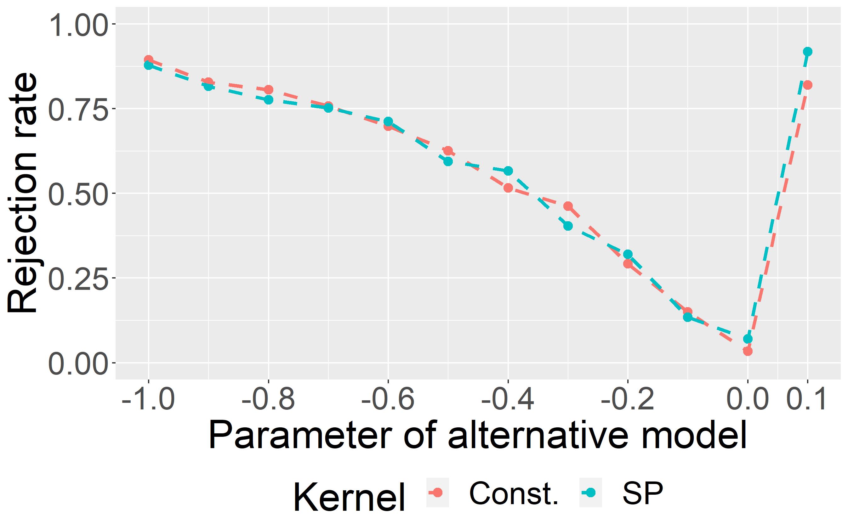
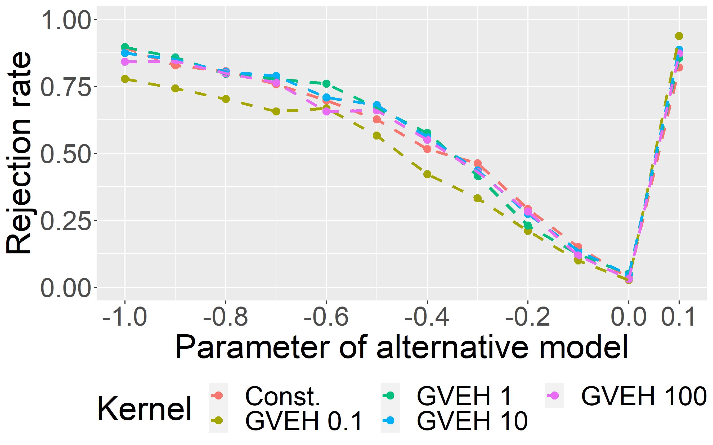
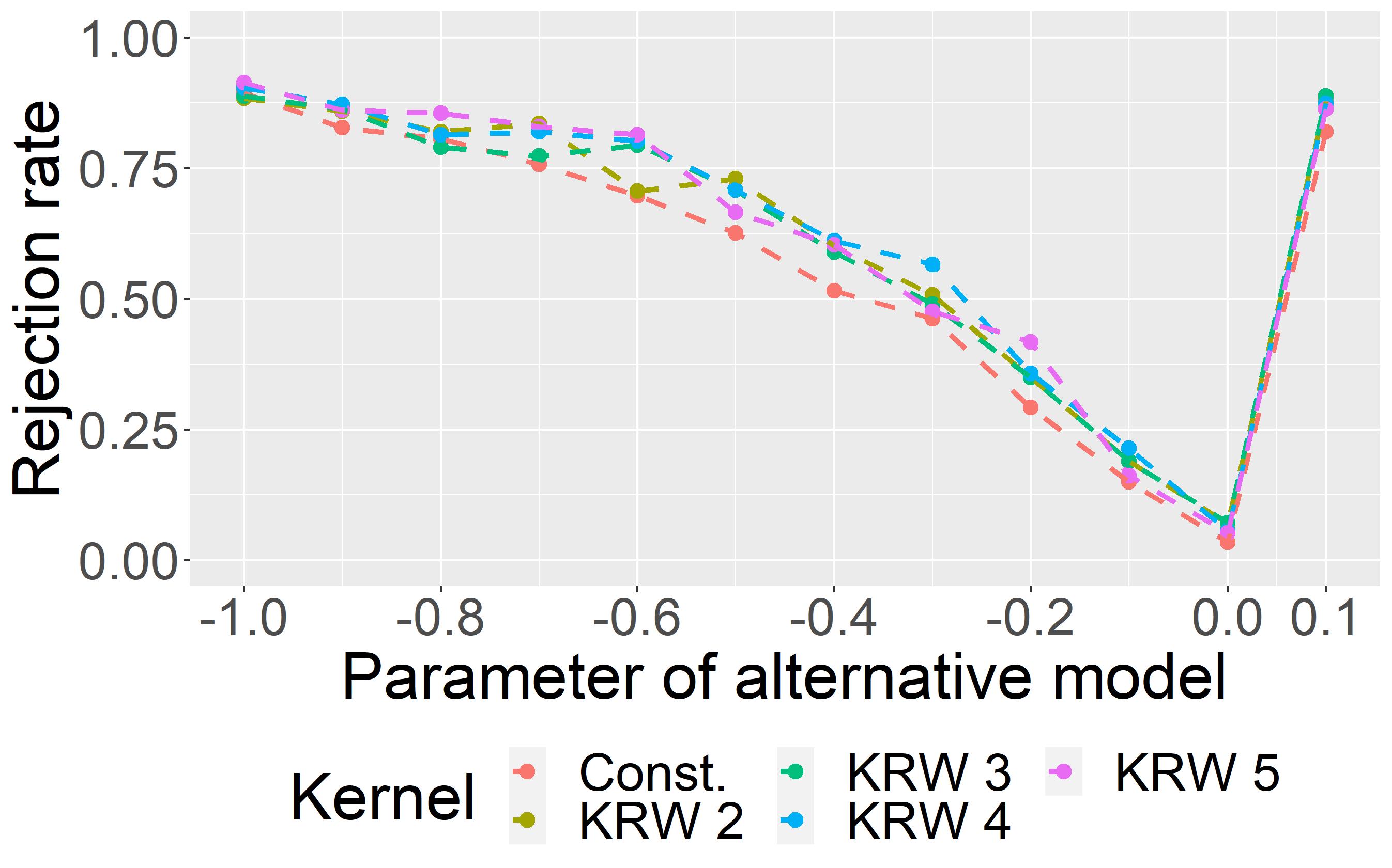
Figure 4: Kernel experiments in the setting of Figure 2: gKSS for E2S model with $\beta_{2}$ perturbed.

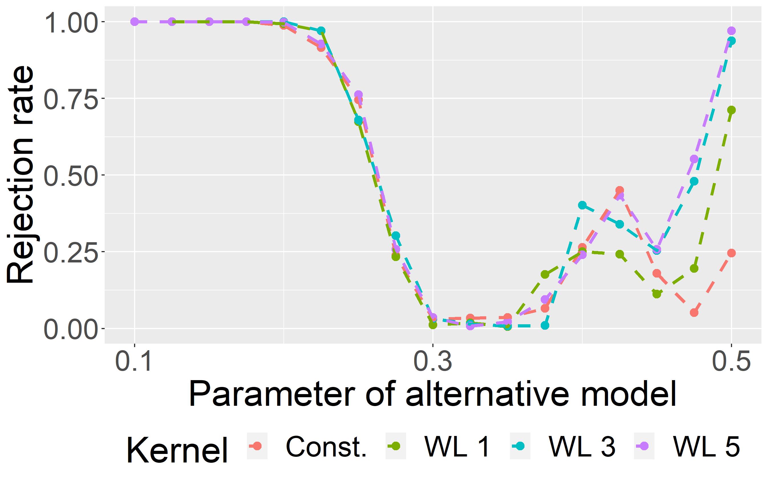
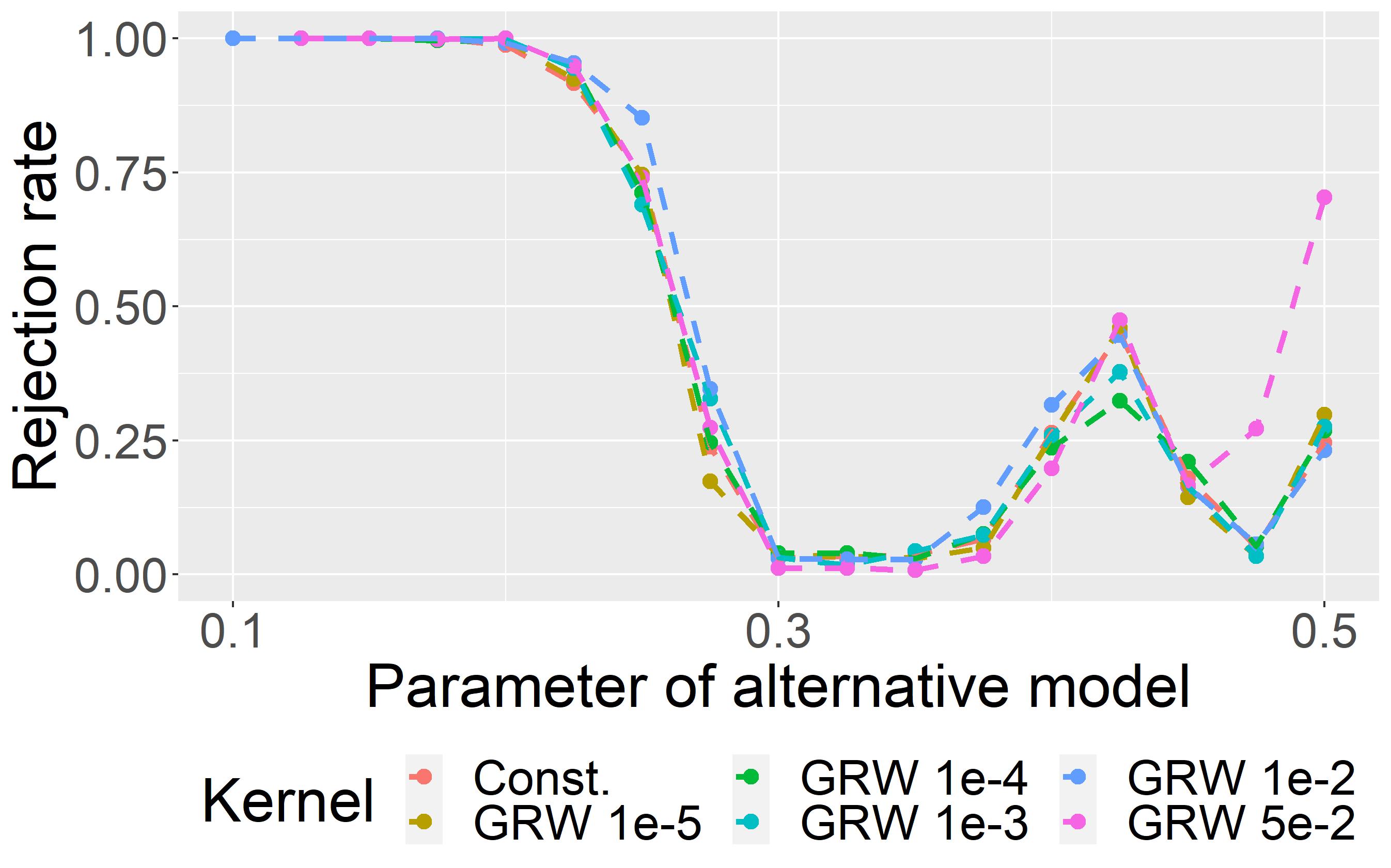
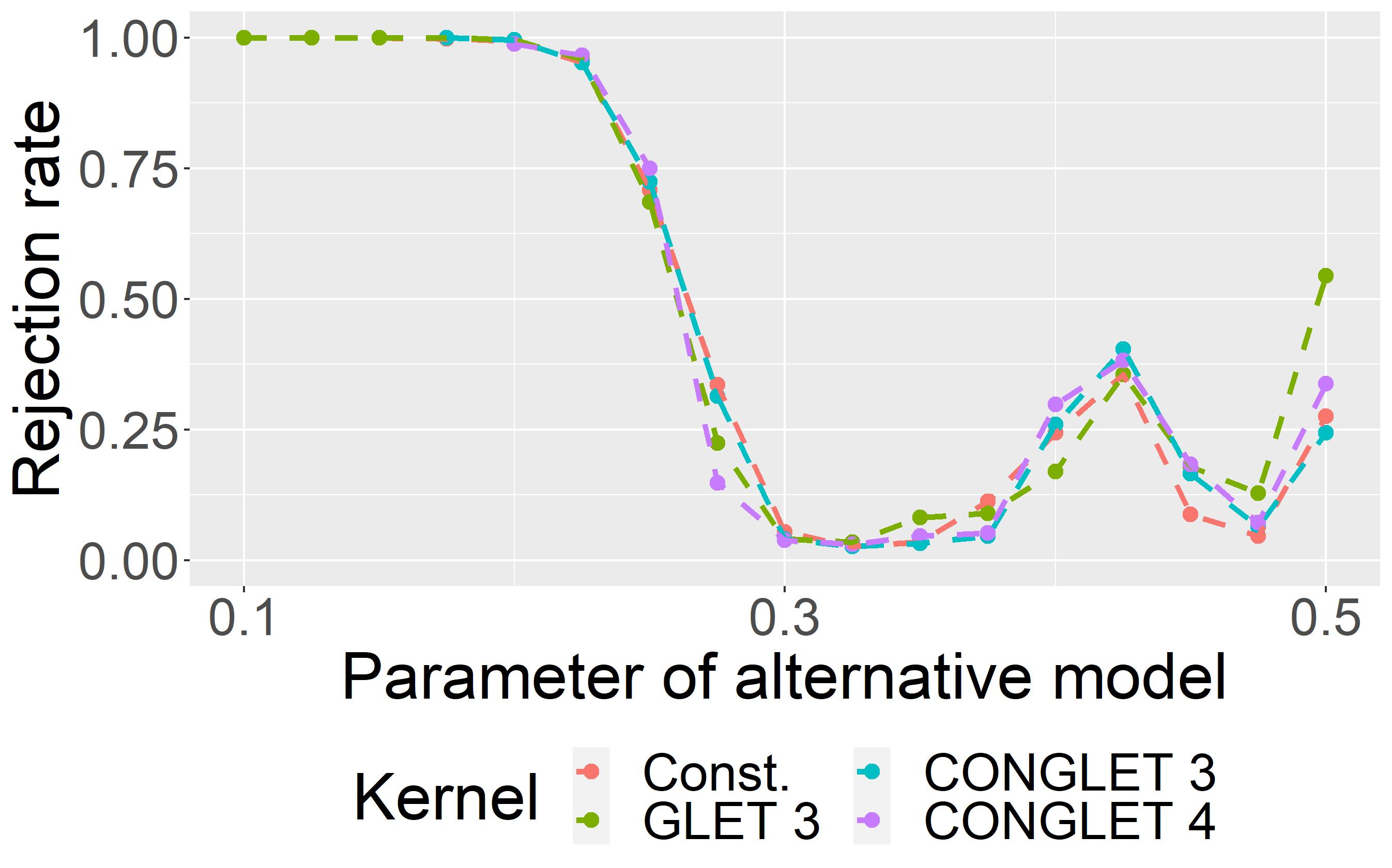
Figure 5: Kernel experiments in the setting of Figure 3: AgraSSt for the GRG model with alternative; $t(x)$ is set to be bivariate (vertex) degree vector.

B.1.1 Additional experiments on the E2S model

In Figure 4, we show the rejection rate for SP, GVEH and KRW kernels in the same E2S setting as presented in Figure 2. All these kernels have similar performance to the constant kernel, with GVEH kernels being more sensitive to parameter choice than the KRW kernels.

B.1.2 Additional GRG experiments: GRG models on the torus

In the main text the results of the experiments using as $t$ the bivariate vertex degree vector are shown. In Figure 6 we show results for using as $t$ the average density in the sample,. The type 1 error is controlled under all kernels; the kernels perform similarly.

Figure 7 shows the behaviour of the kernels using the common neighbour statistic. The behaviour is similar to the bi-degree statistic, in showing an additional dip. The constant kernel and the shortest path kernel have lowest rejection rate not at the true value. The connected graphlet kernel with graphlet size 3 also suffers from this issue.

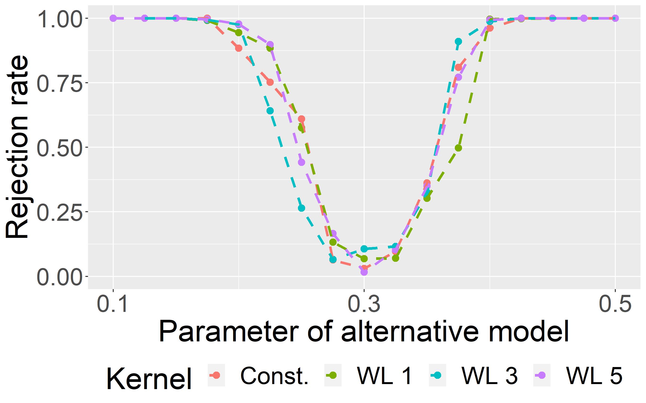
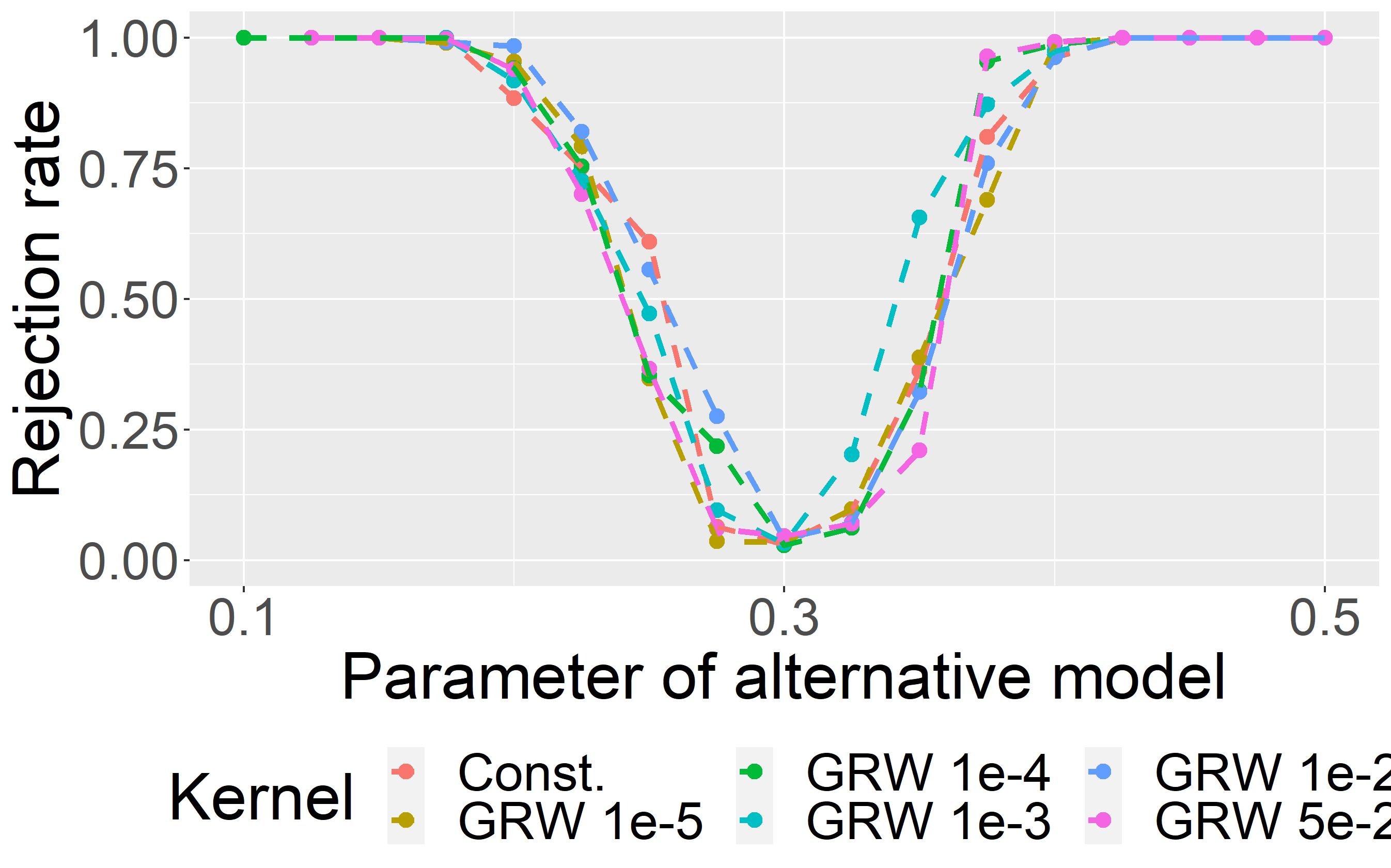
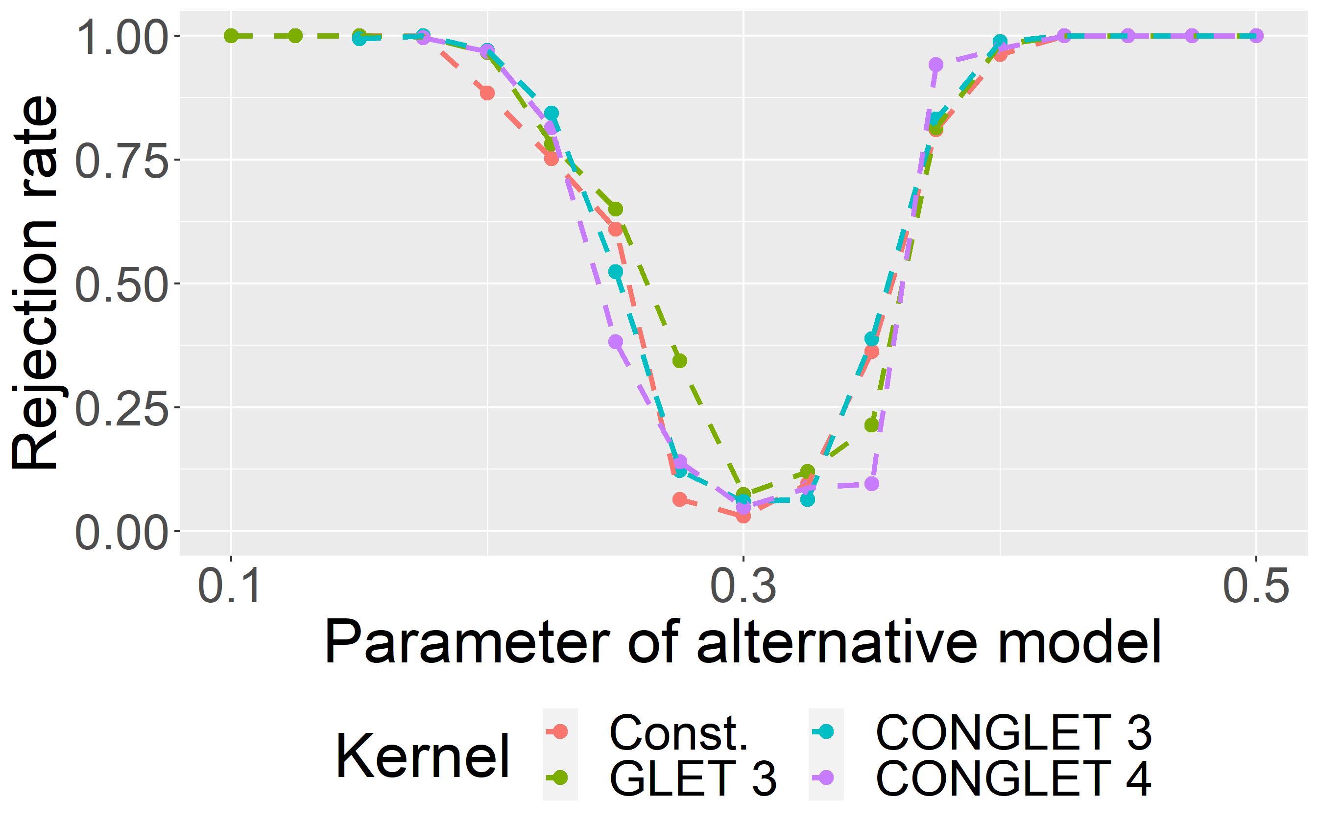
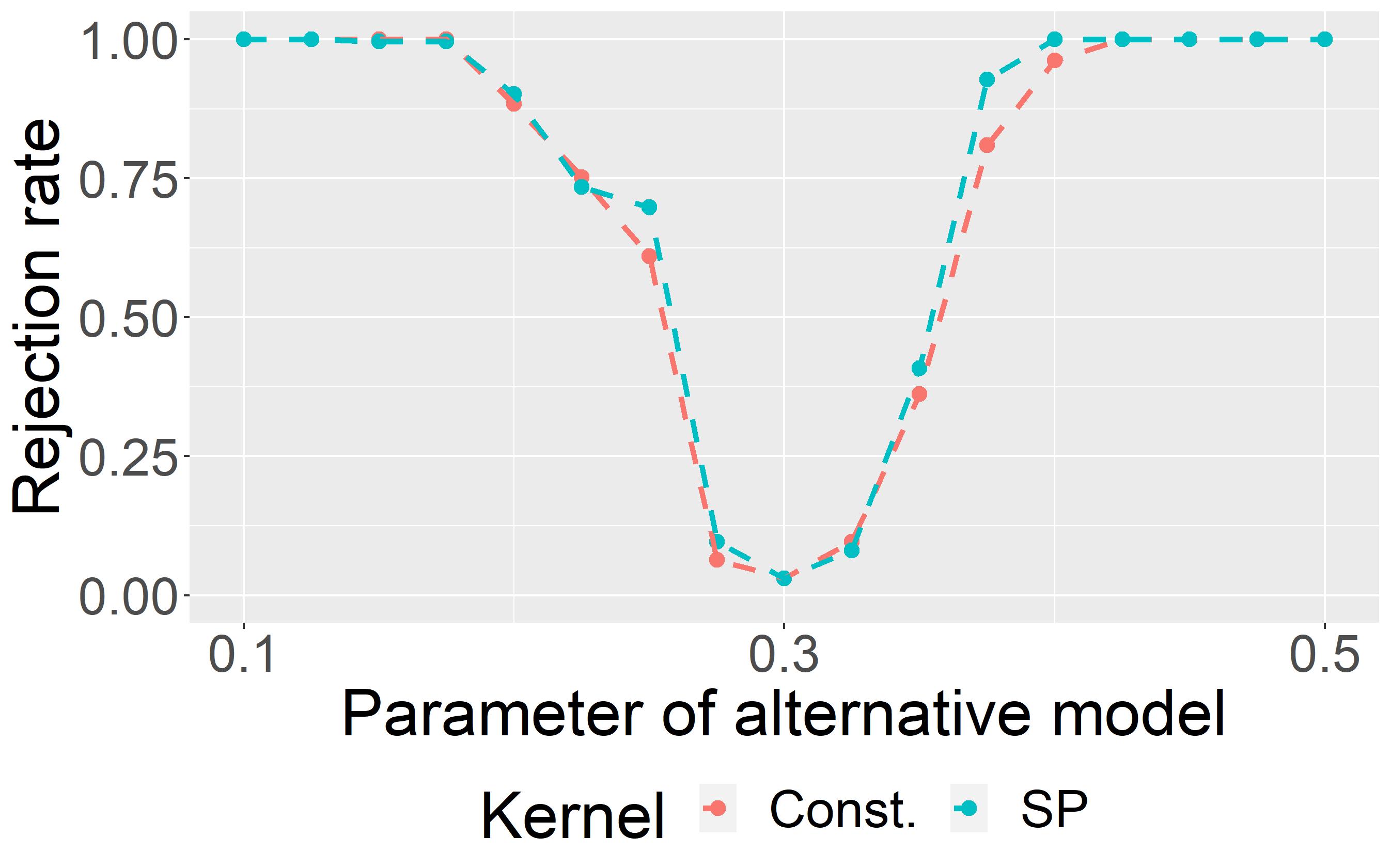
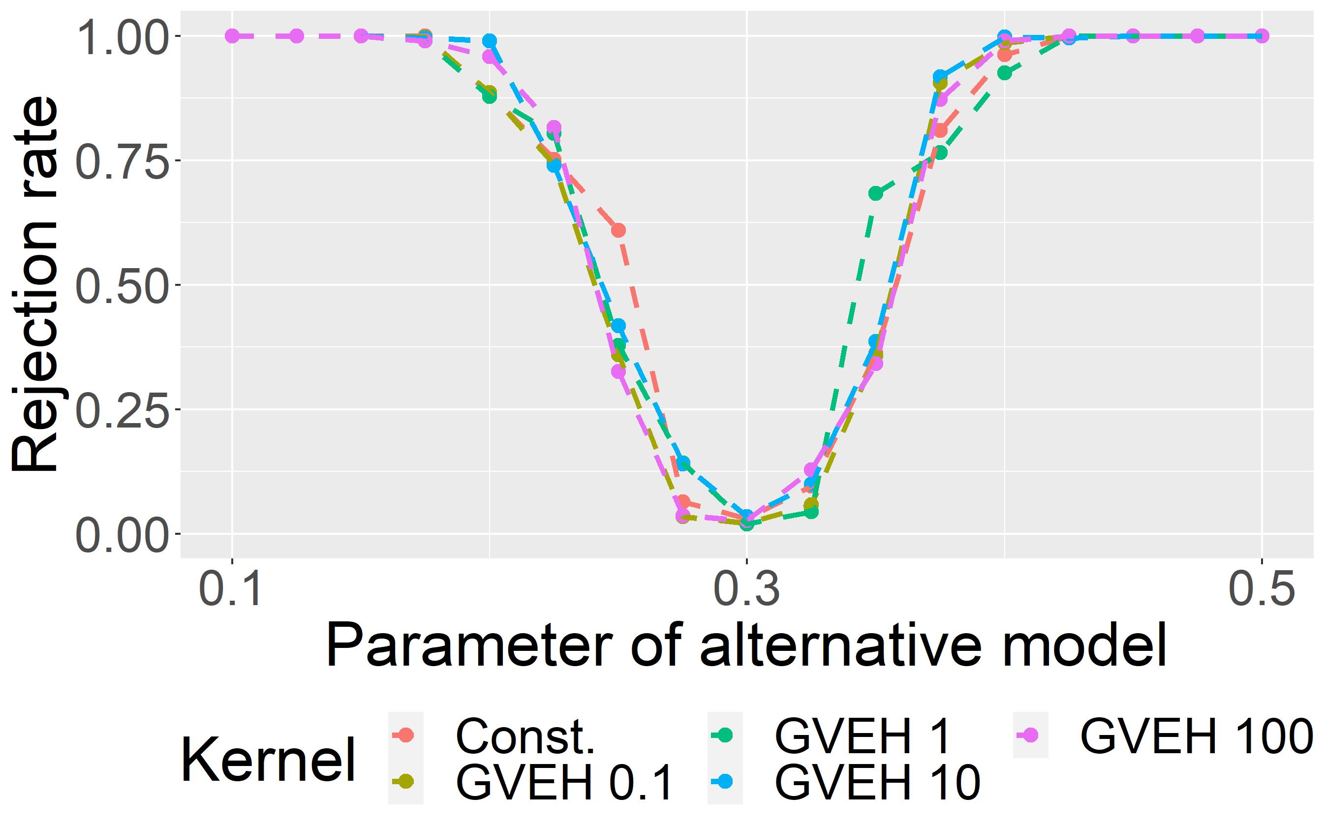
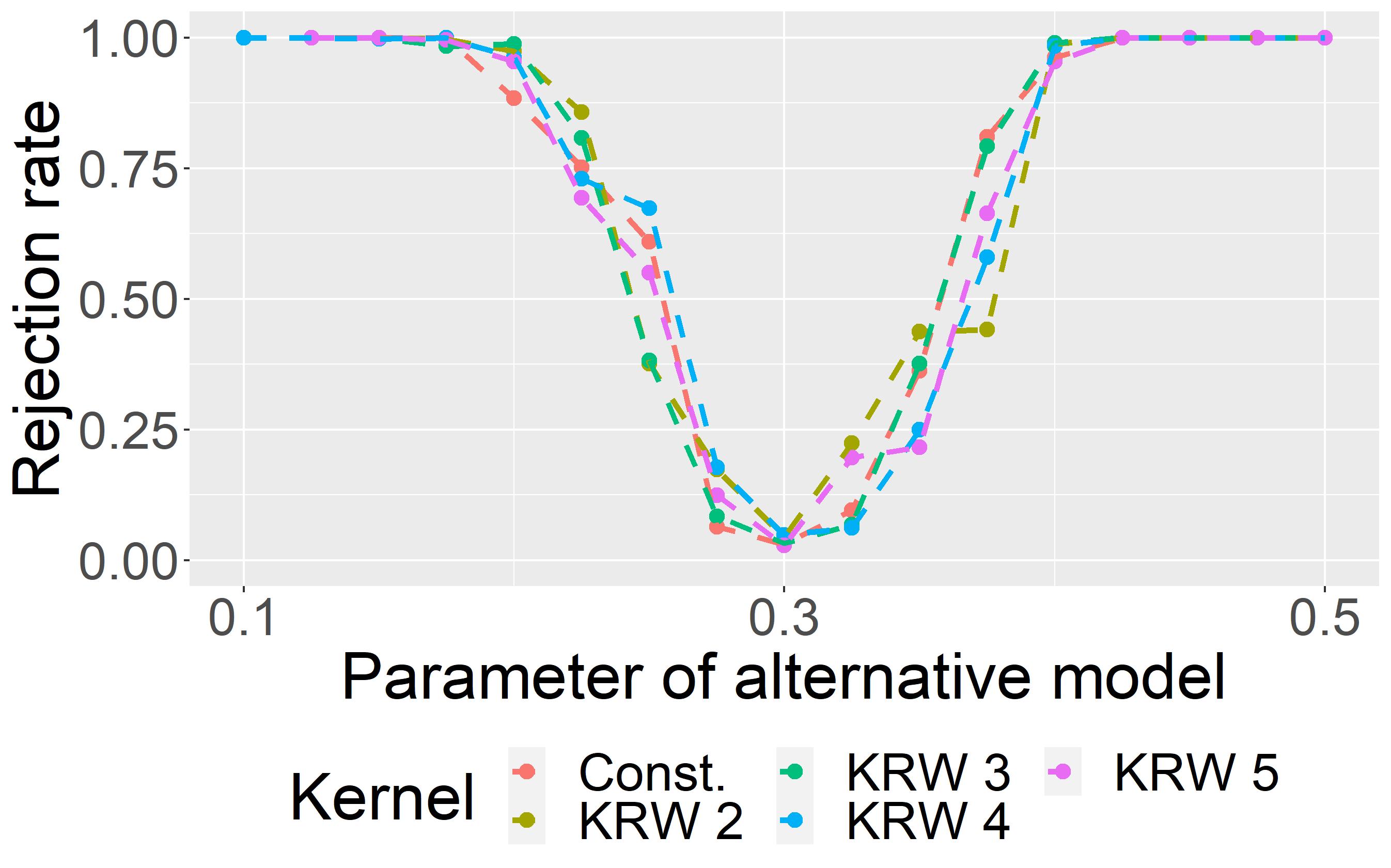
Figure 6: AgraSSt for the GRG model with $t(x)$ being the edge density.

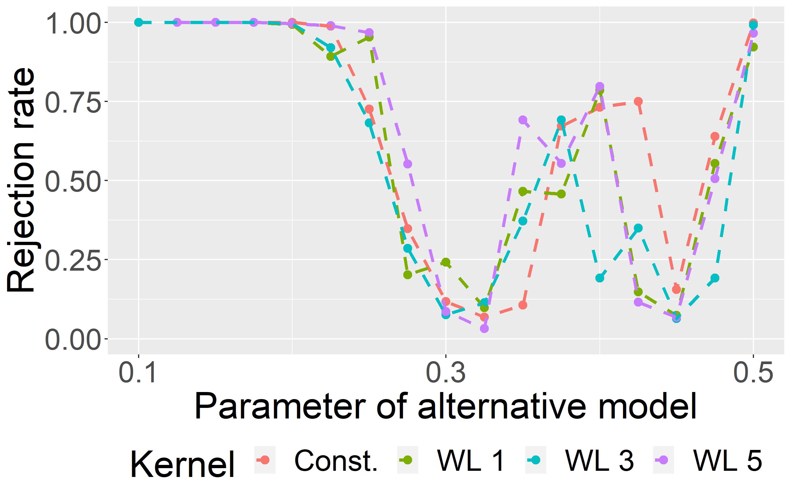
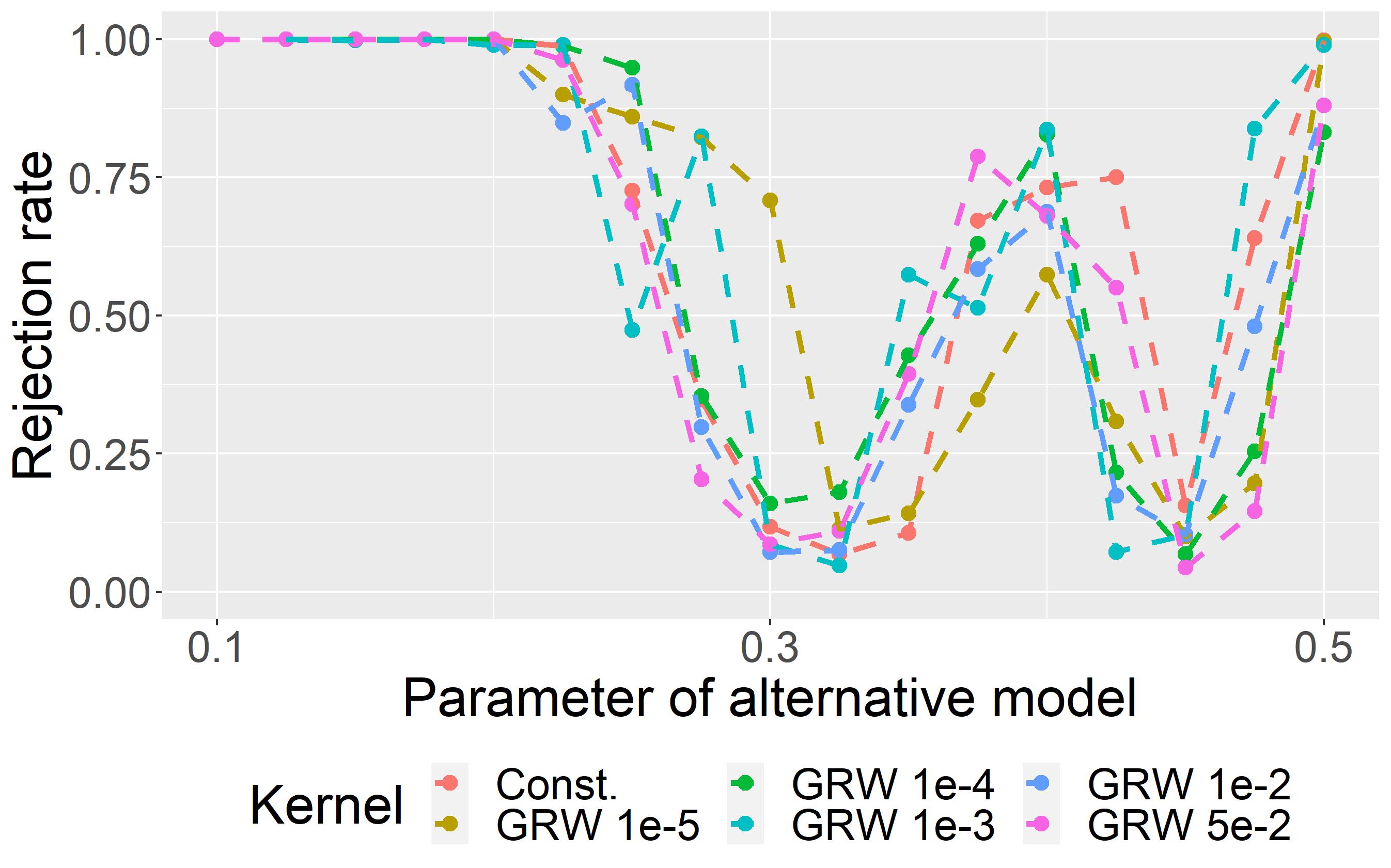
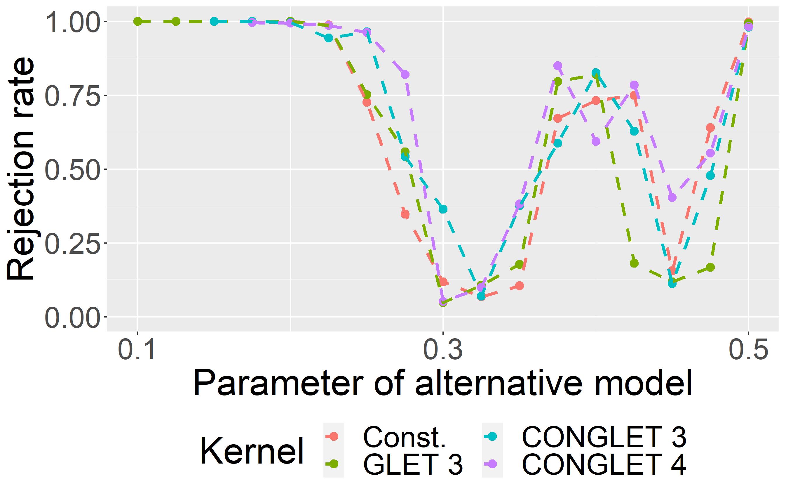
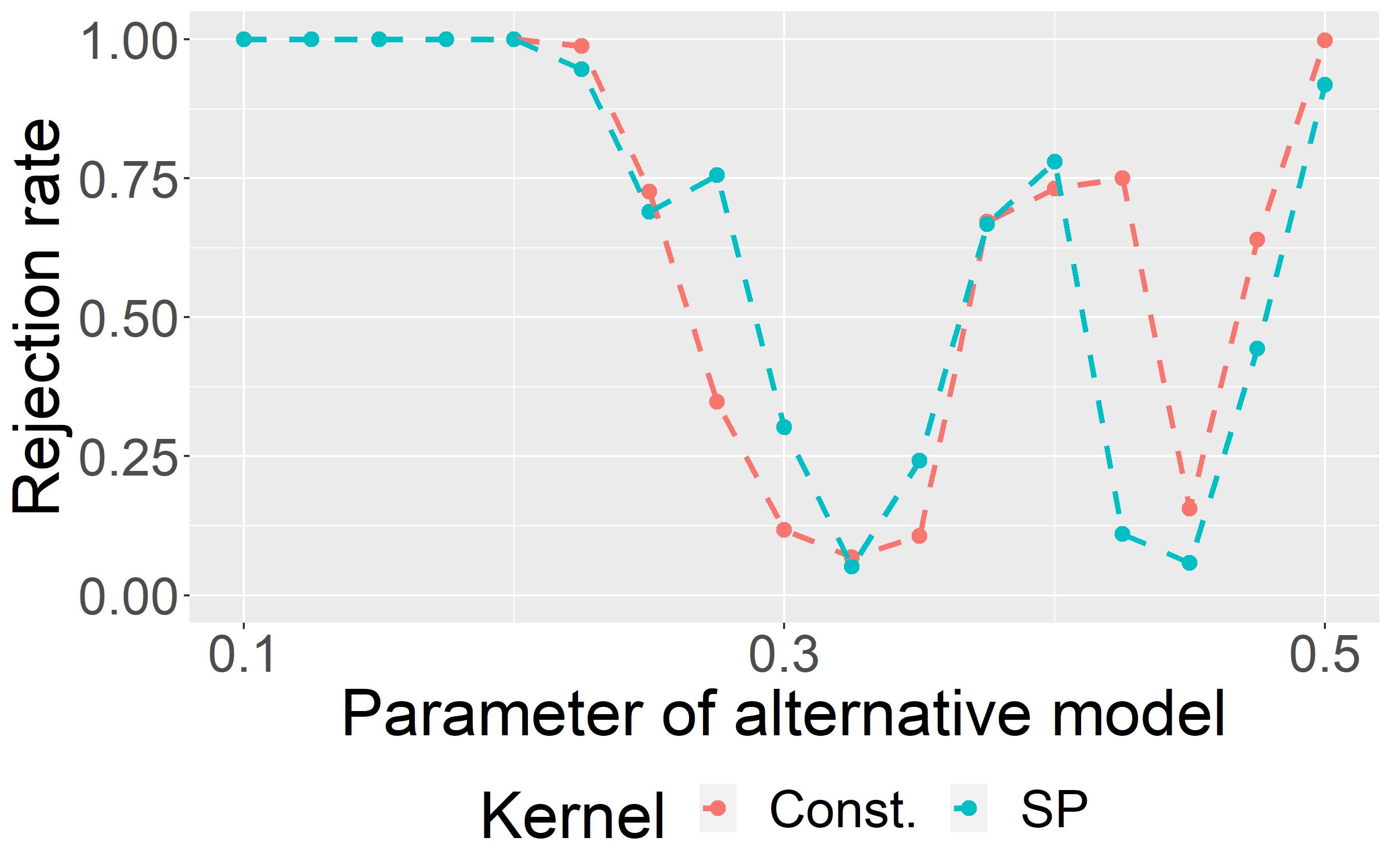
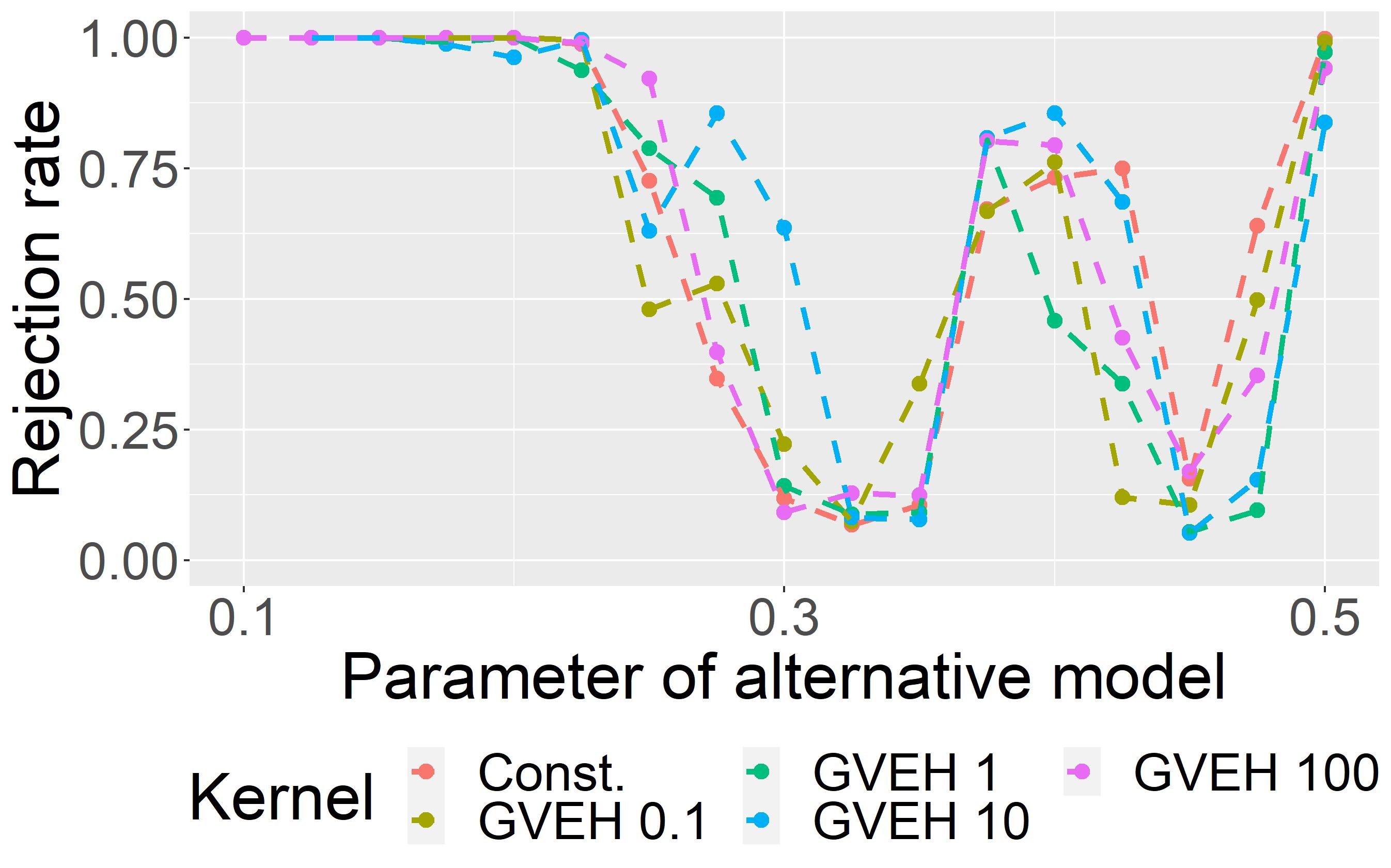
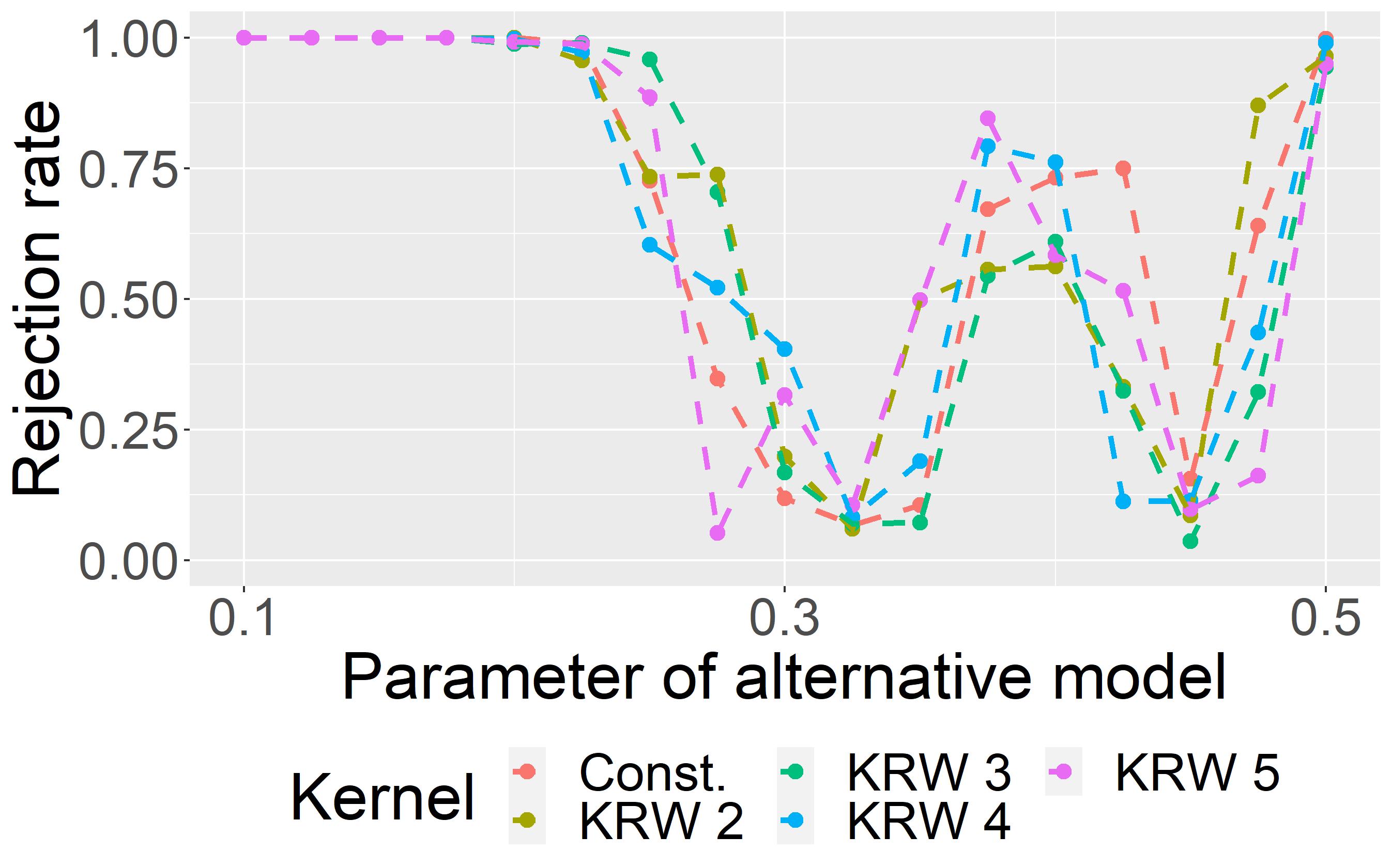
Figure 7: AgraSSt for the GRG model with $t(x)$ being the number of common neighbours.

B.1.3 Additional GRG experiments: GRG models on a unit square

In the next set of experiments, instead of on a torus, we place the vertices on the 2-dimensional unit square to generate the geometric random graph models. The null model has radius $r=0.3$ while the alternative models have a different $r$. Experimental results with AgraSSt are shown in Figure 8, Figure 9 and Figure 10. In this example all the tested kernels show a similar behaviour, with sparse alternatives easier to distinguish than denser alternatives.

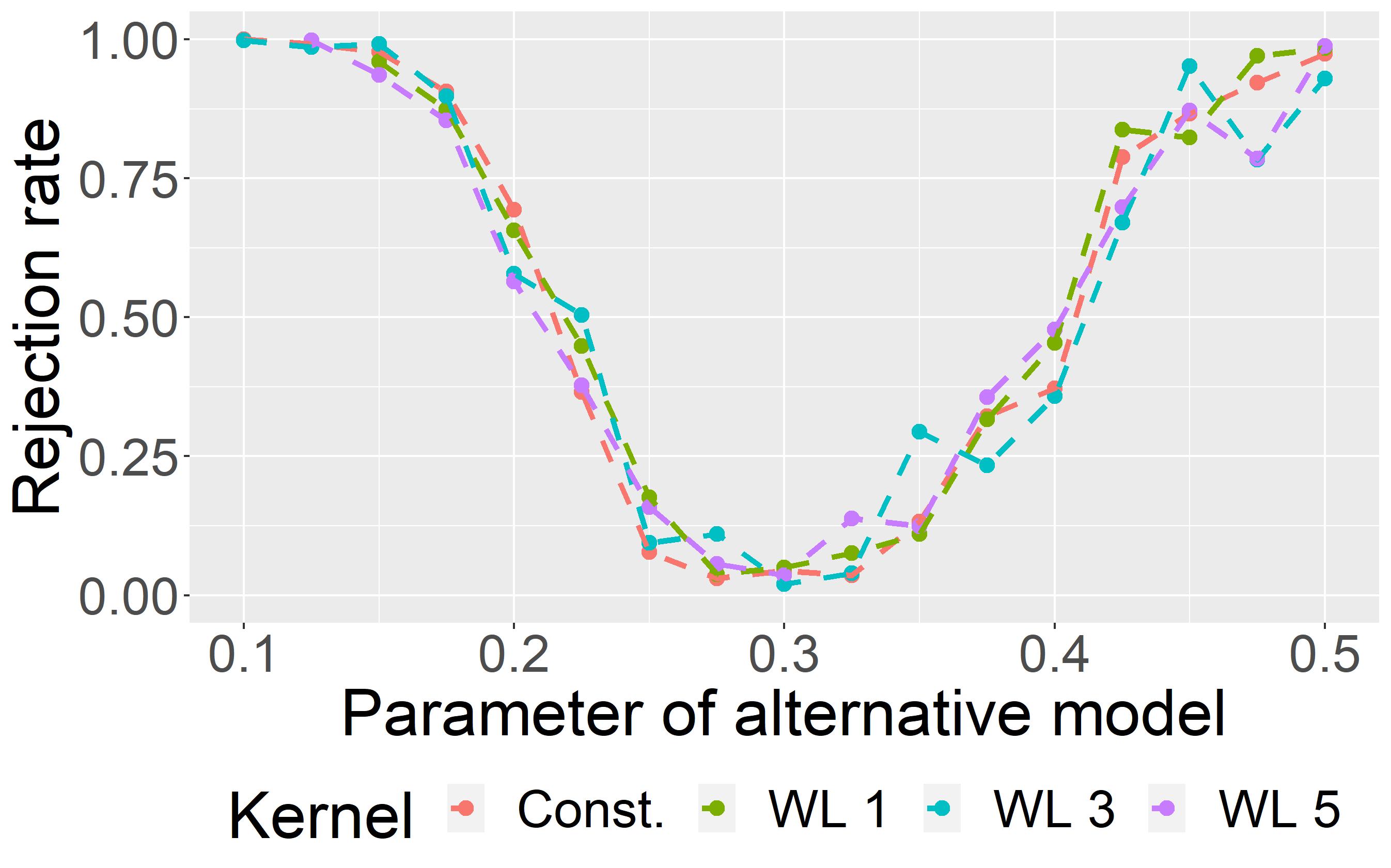
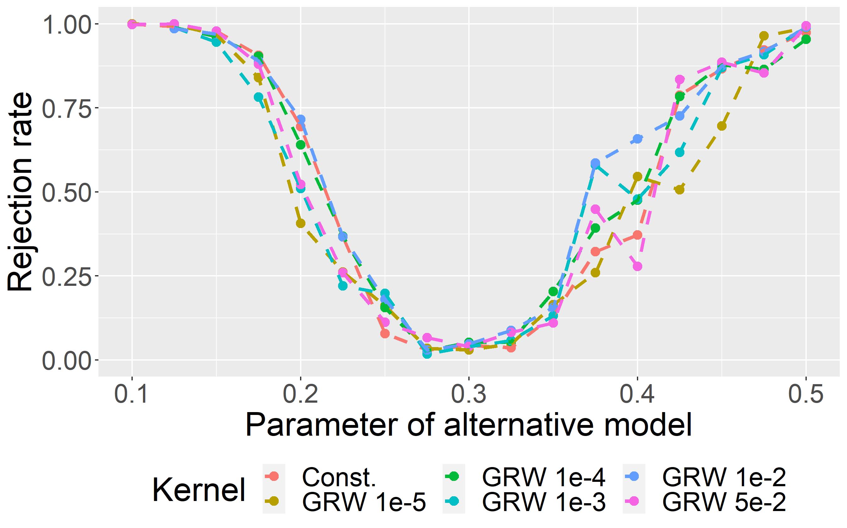
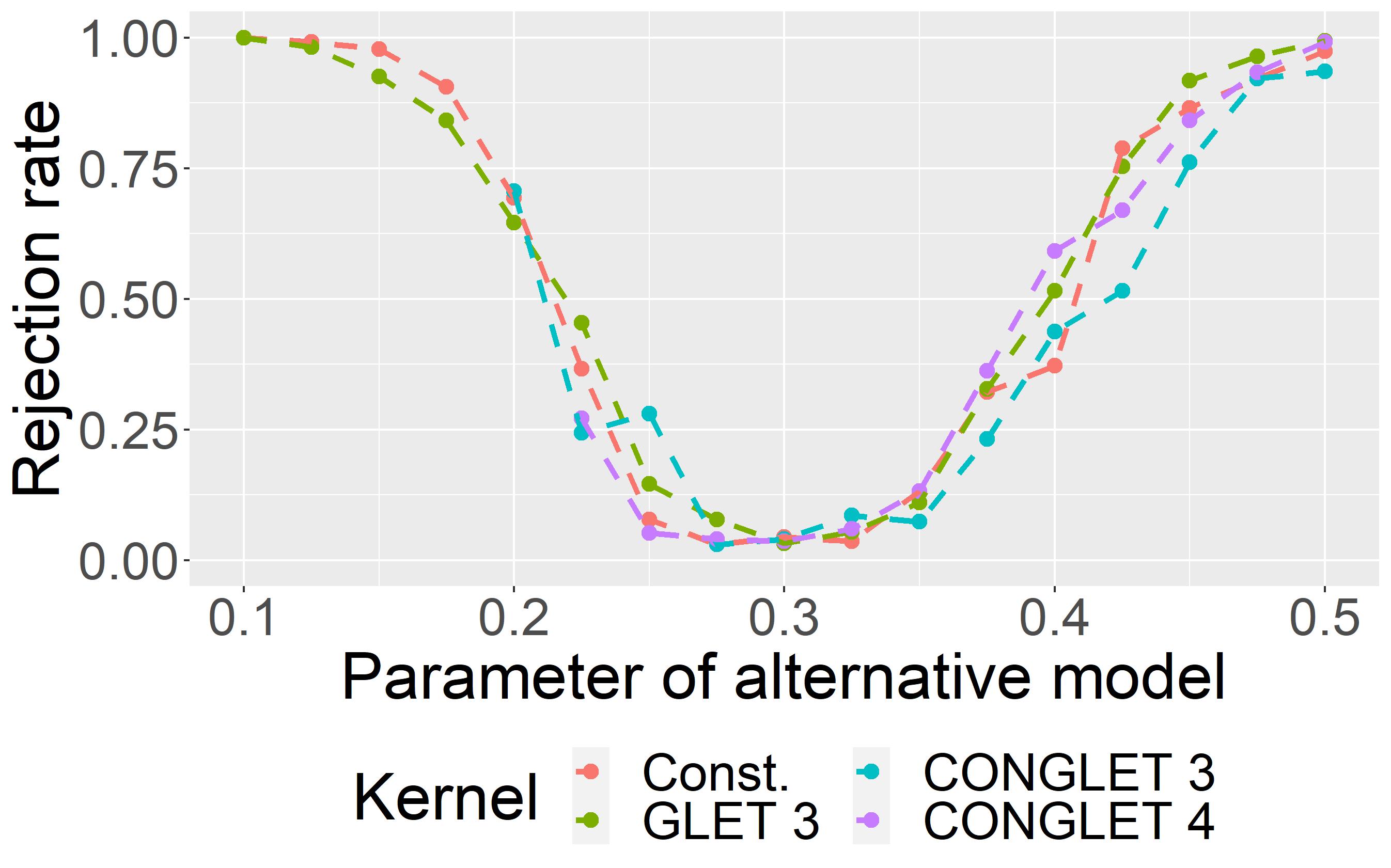
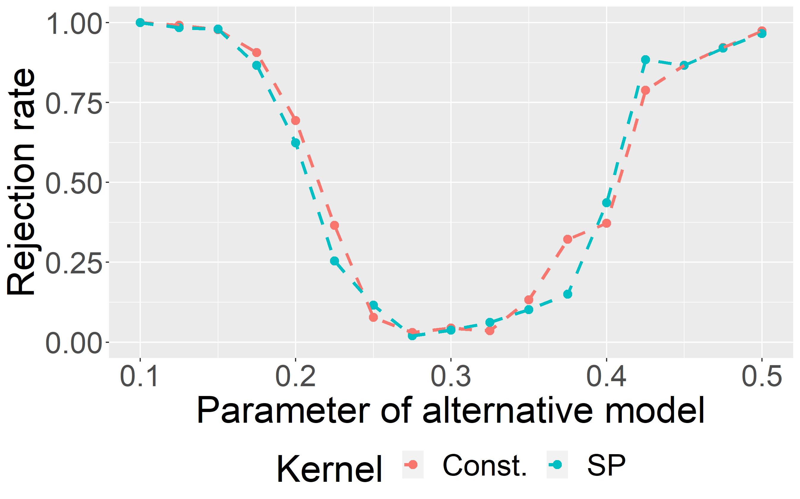
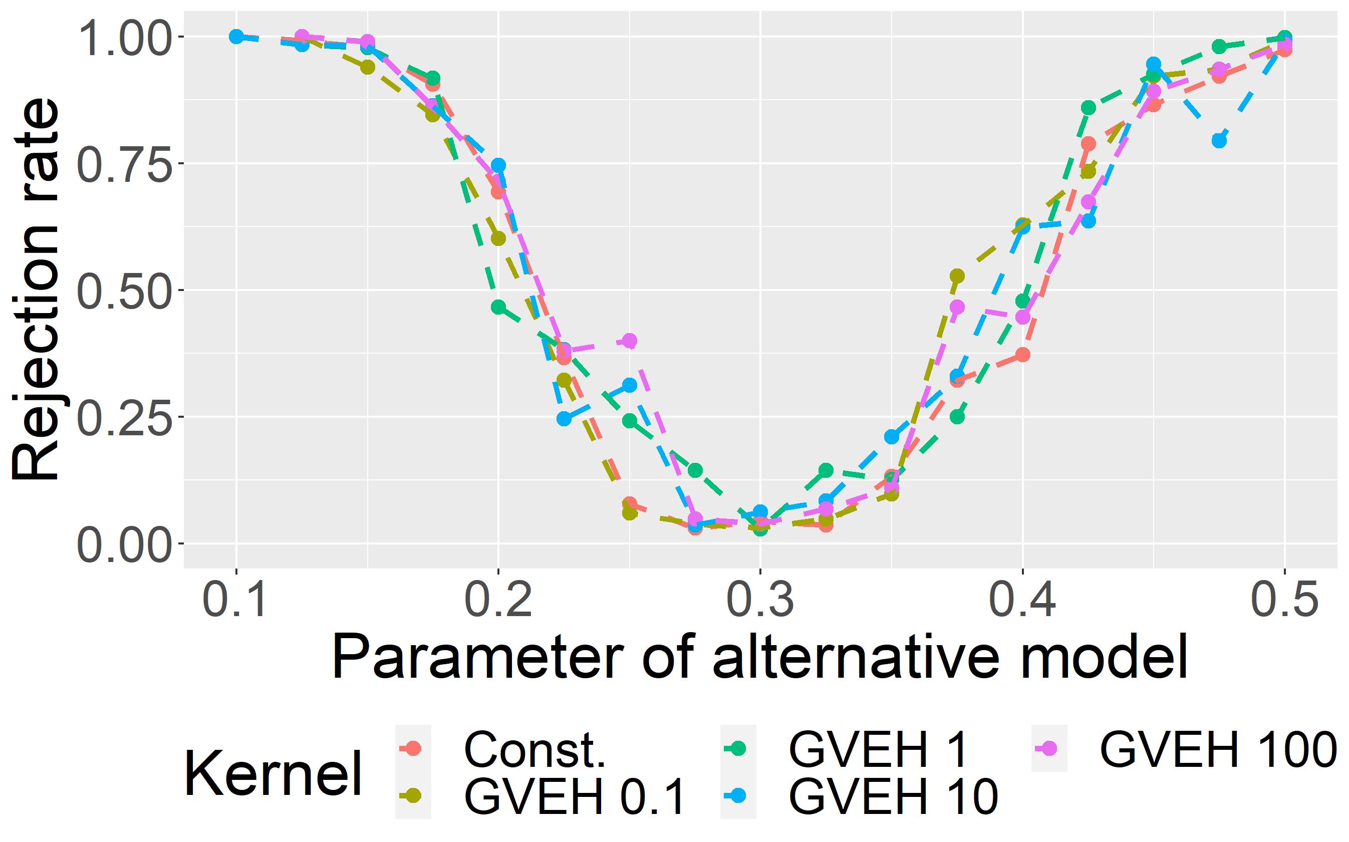
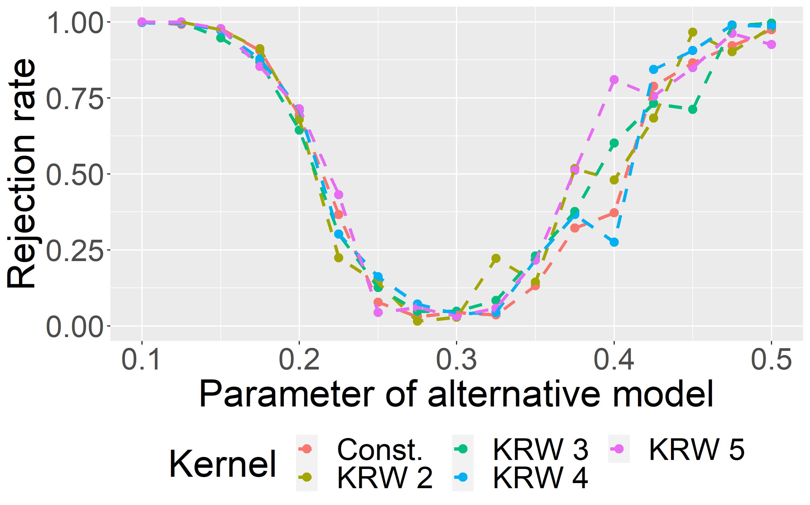
Figure 8: AgraSSt for GRG on the 2-dimensional unit square with $t(x)$ being the edge density.

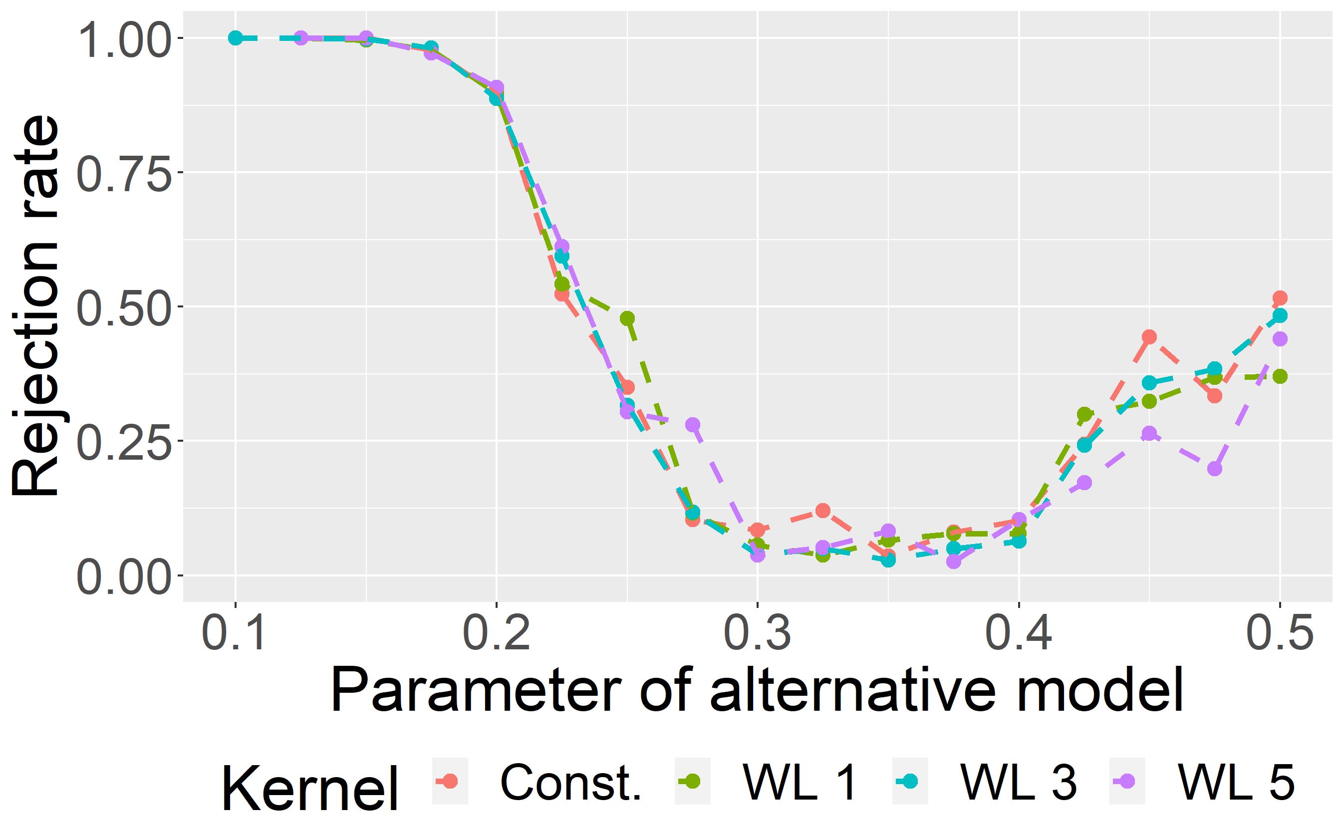
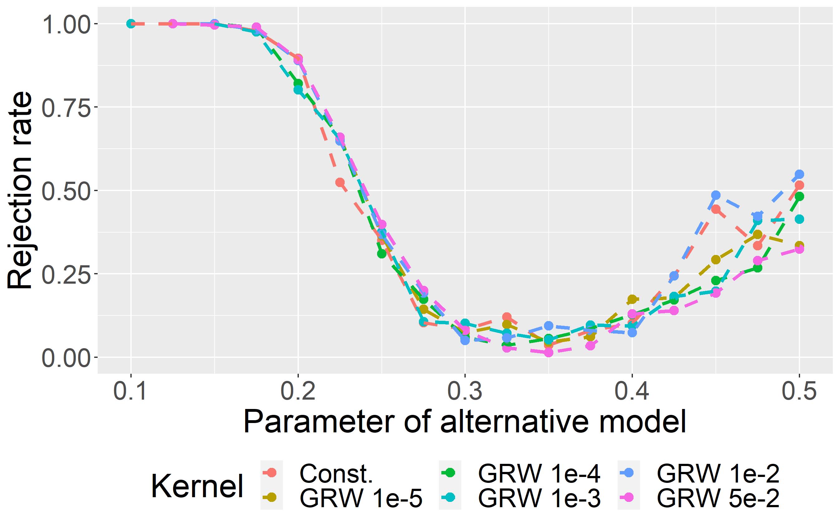
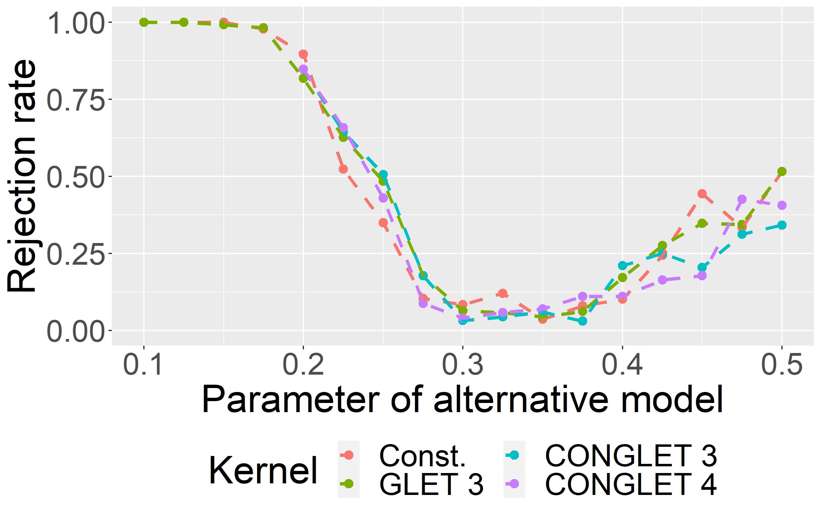
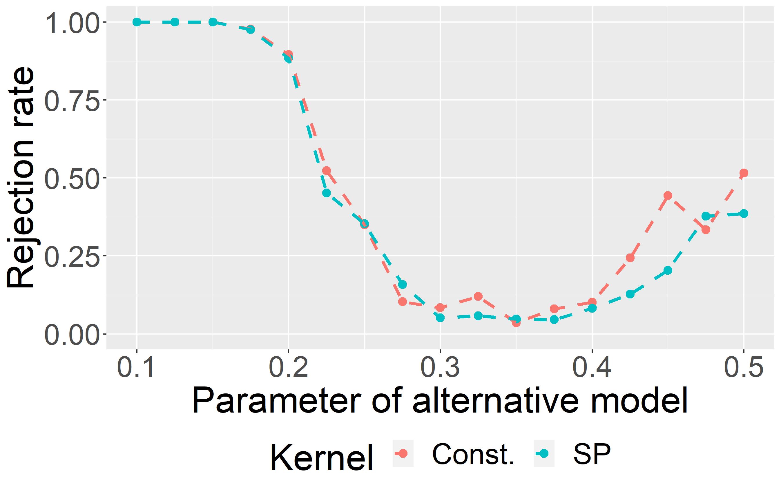
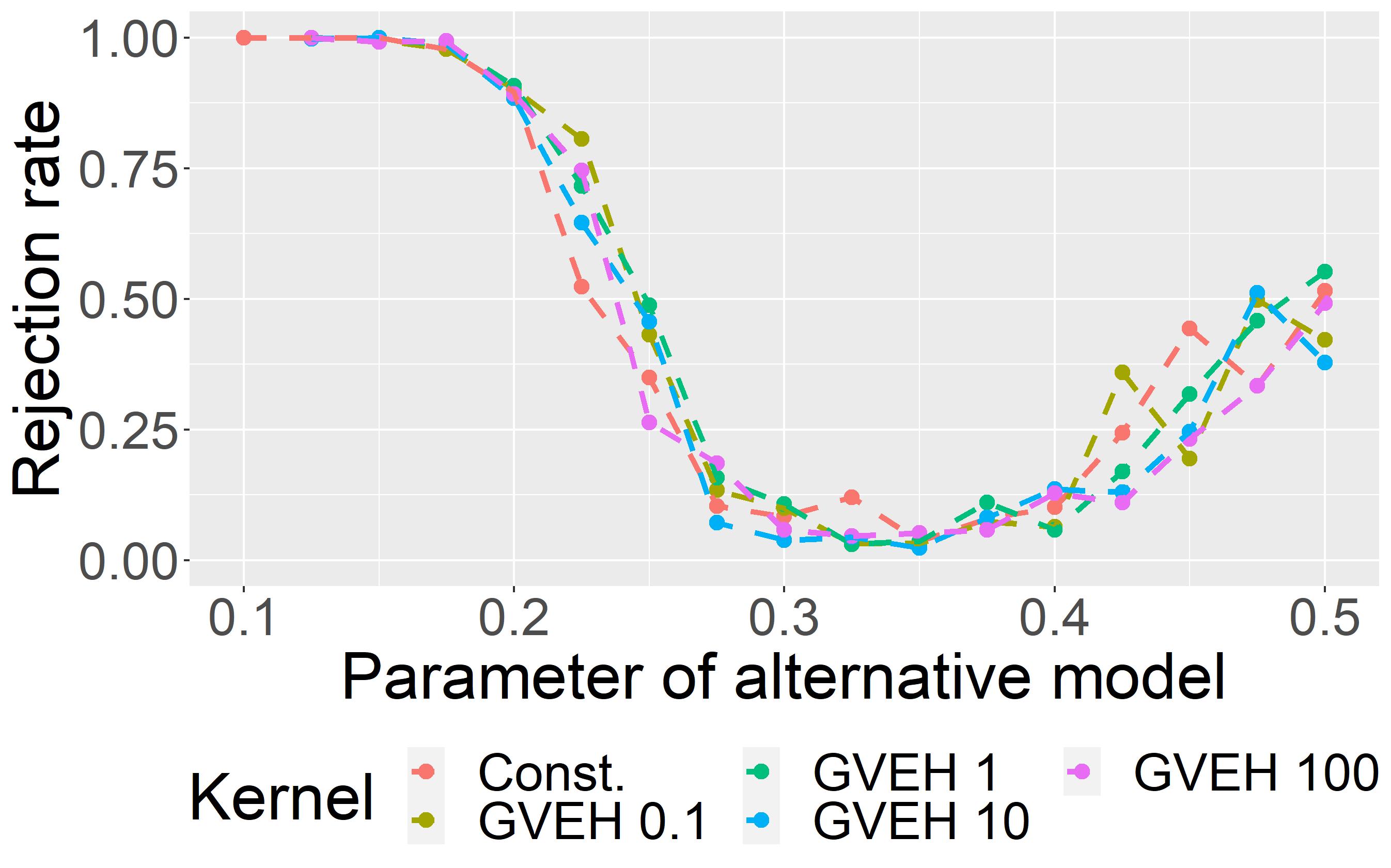
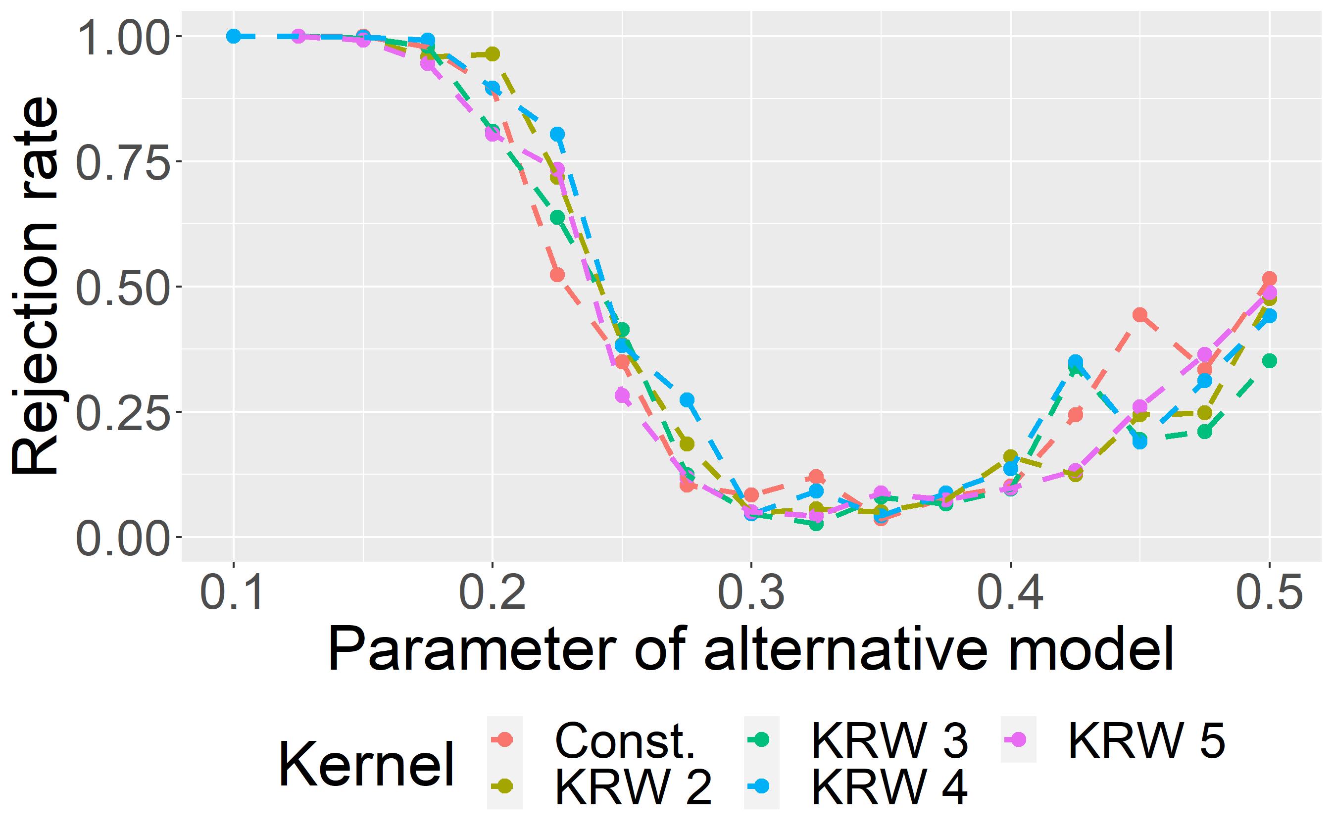
Figure 9: AgraSSt for GRG on the 2-dimensional unit square with $t(x)$ being the bivariate degree vector.

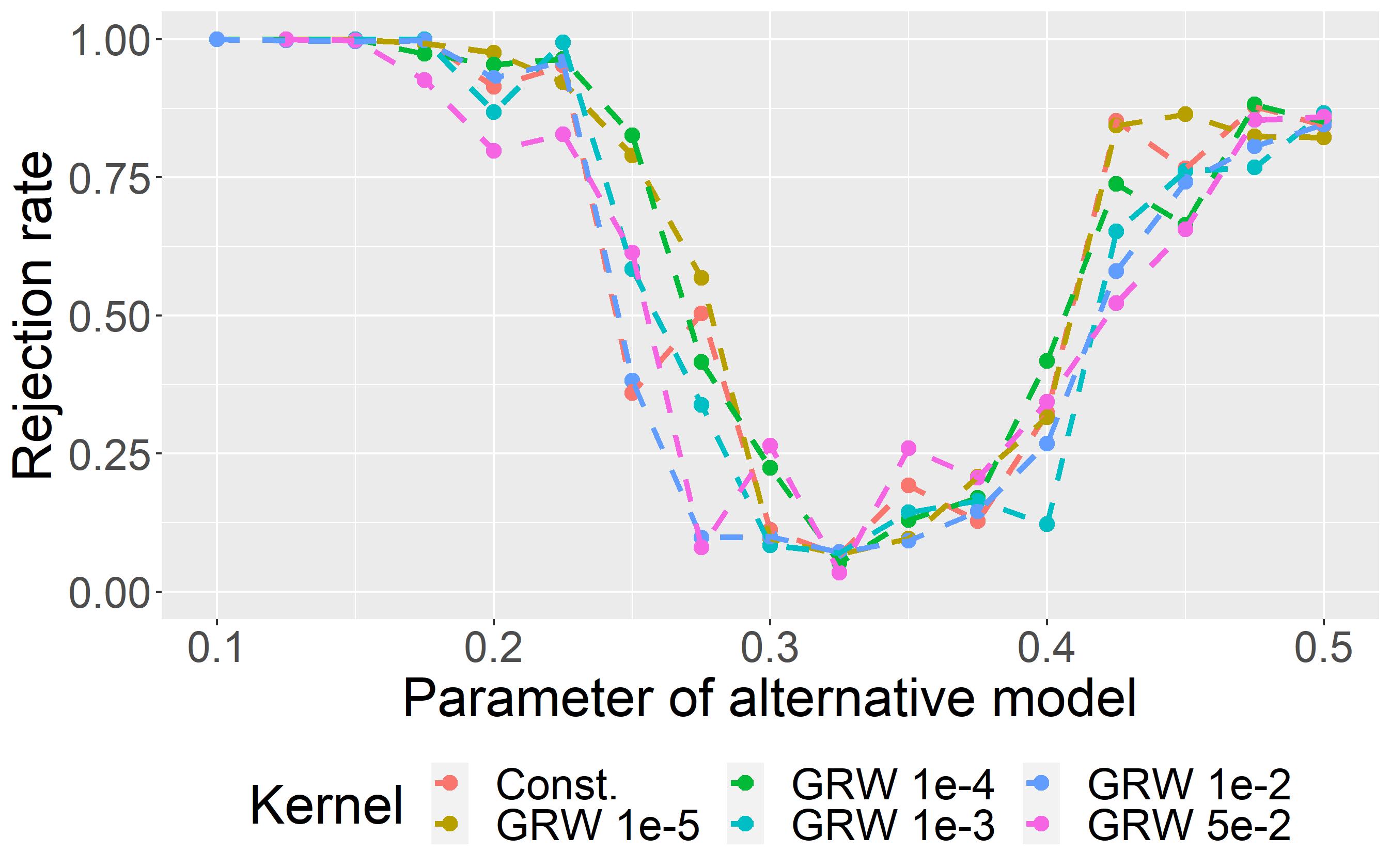
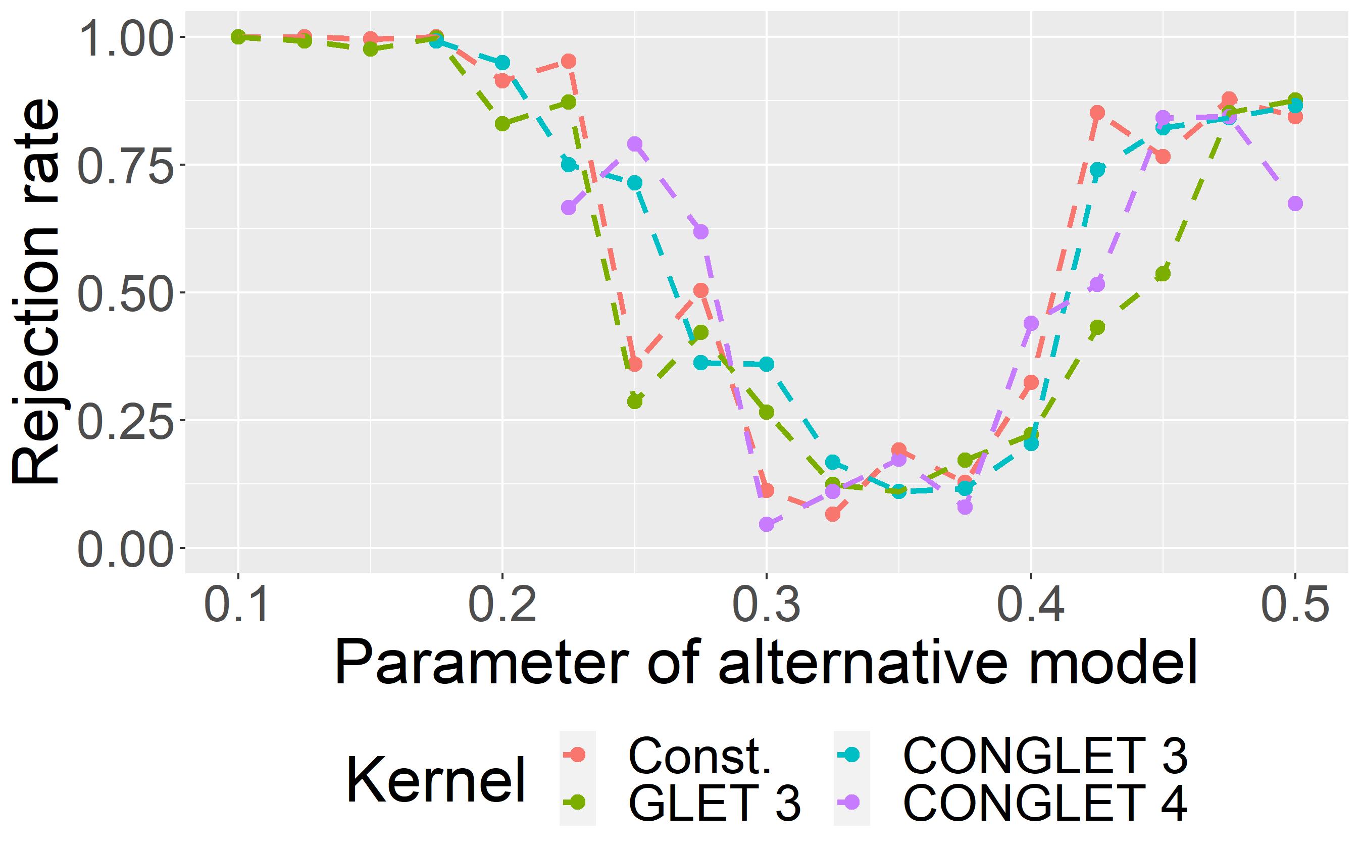
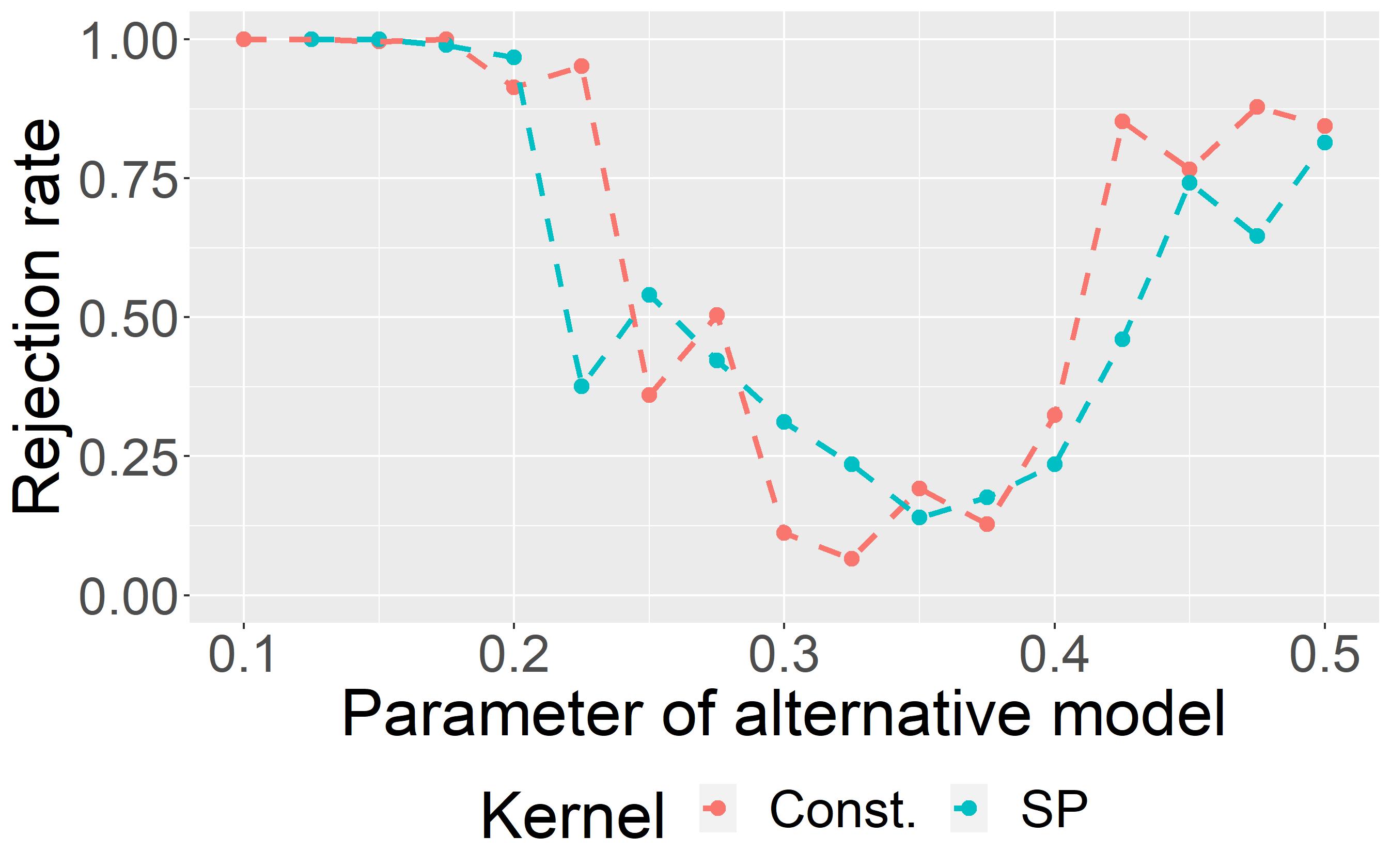
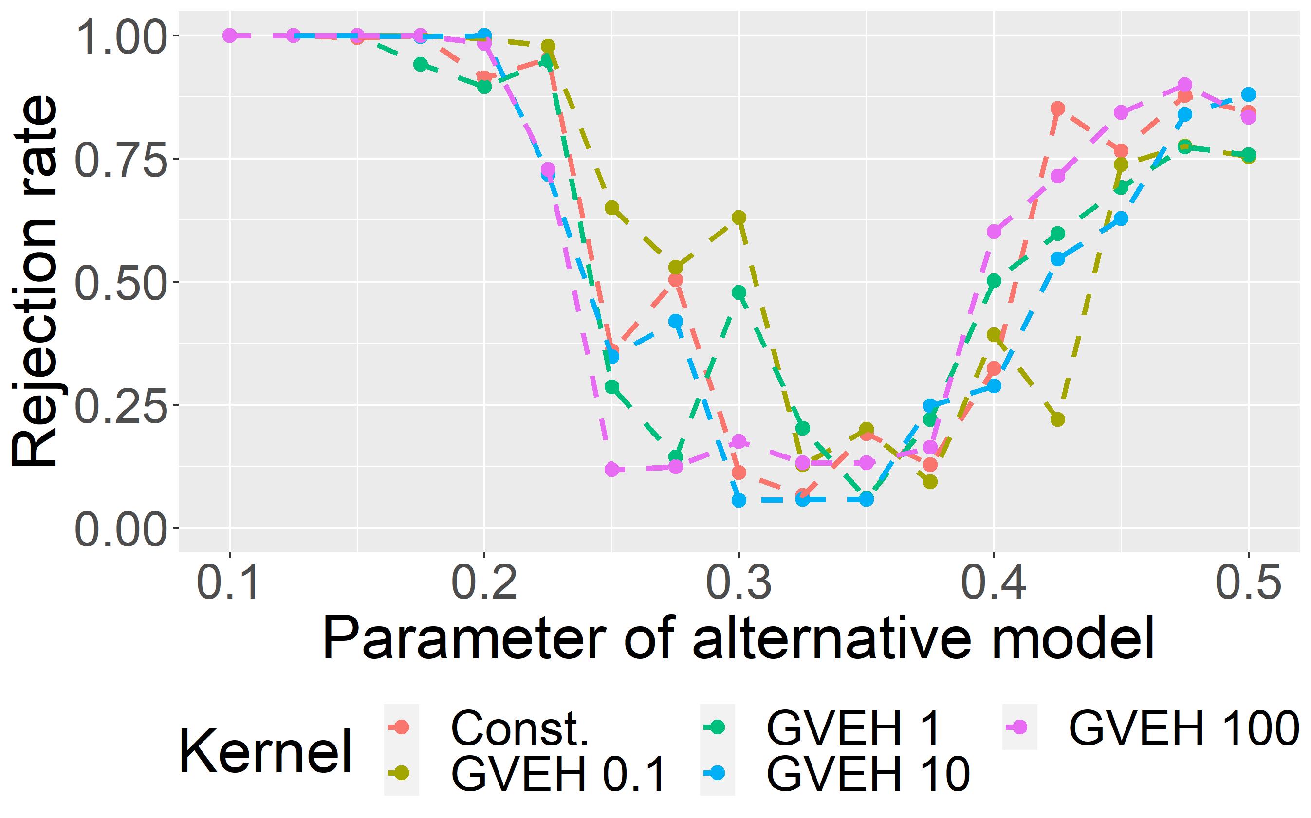
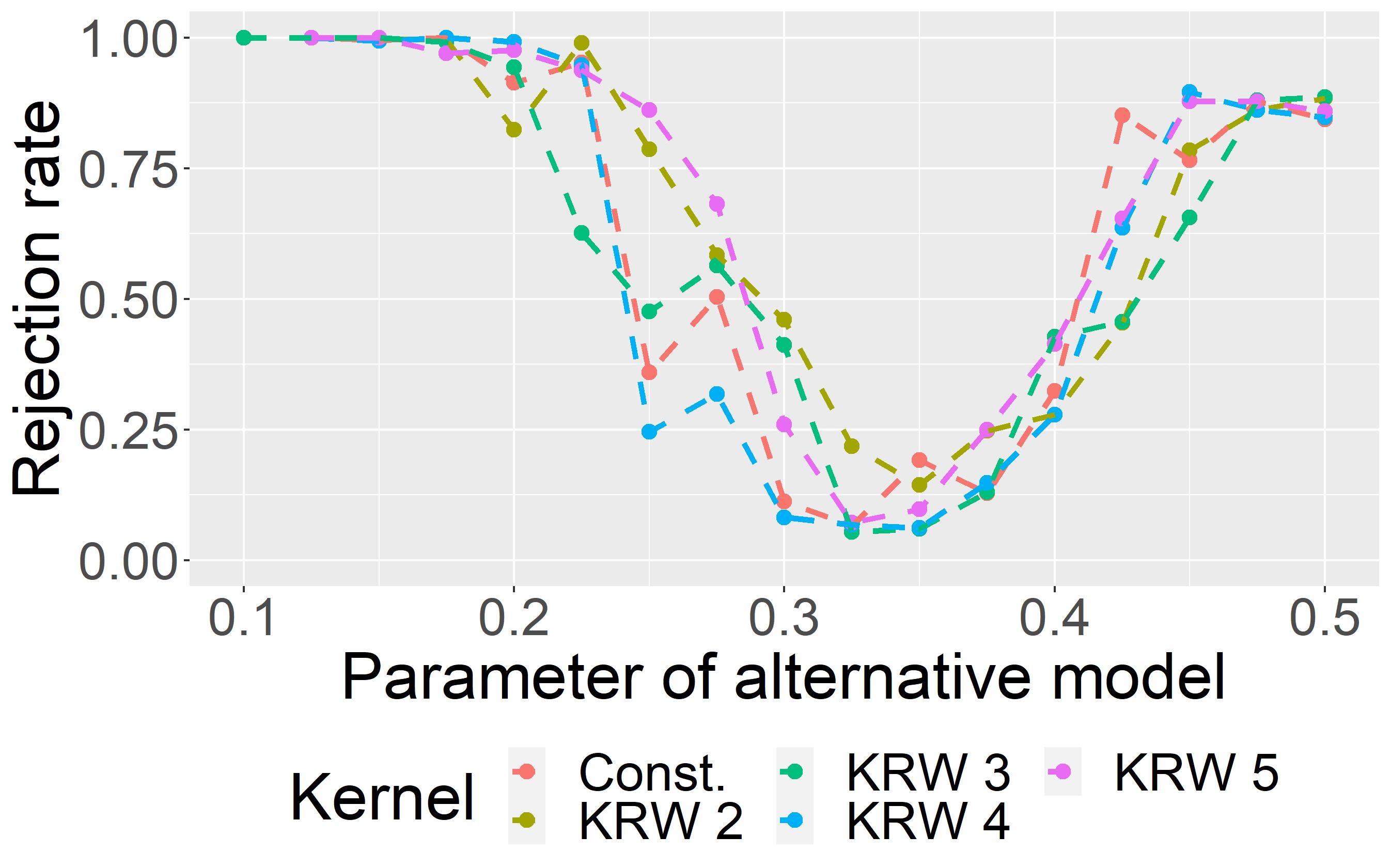
Figure 10: AgraSSt for GRG on the 2-dimensional unit square with $t(x)$ being the number of common neighbours.

B.1.4 AgraSSt for geometric random graphs on a torus: further details

For the geometric random graph on a torus, we observe a spike and subsequent dip for the bidegree statistic as well as for the common neighbour statistic, which occurs at around $r_{M1}=0.45$. We hypothesize that this phenomenon stems from the torus structure of the underlying space; the behaviour on the unit square does not show this pattern. The torus effect can be most easily seen for the common neighbour statistic. Consider two vertices placed on the unit square and imagine circles around these vertices of radius $r$, as in Figure 11. The area of their intersection equals the probability that a randomly placed vertex is a common neighbour of the two. For small $r$, this area is large if the vertices are very close to each other and small or zero if the vertices are far apart. Hence, conditional on two vertices having a common neighbour the probability that two vertices are only a distance smaller than $r$ apart is large, and thus the probability that they are themselves connected is large as well. However, for larger $r$, the area of overlap can be large even though both vertices are far away due to the circles wrapping around the torus (see Figure 11). Thus, the information about the number of common neighbours may become less informative for larger radius $r$.

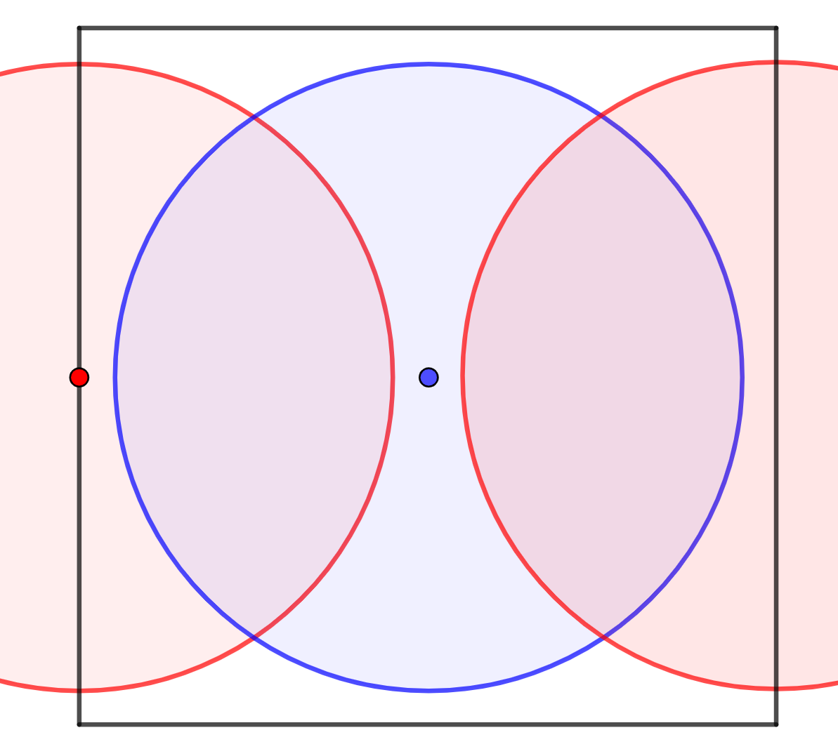
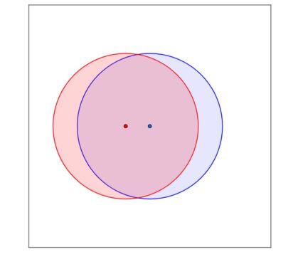
Figure 11: Two vertices, in red and blue, and corresponding surrounding circles of radius are displayed: left for $r=0.45$, right for $r=0.3$. Left: Even though the vertices have a distance of $0.5$ and are not connected in the Geometric Random Graph with radius $r=0.45$, their area of overlap is quite large because the red circle extends over the boundary of the unit square. Without the torus structure, the area of overlap between the two circles would only be half as large. Right: Here $r=0.3$ and the two vertices are connected in the Geometric Random Graph model; the overlap of the two circles around them is similar in size to the overlap on the left-hand side. Thus, based on the overlap alone the two models are difficult to distinguish.

This effect does not occur in the geometric random graph model on the two-dimensional unit square in the Euclidean space as the circles do not wrap around the edges of the square. Thus, compared to the torus topology, the area of overlap differs more depending on whether vertices are close or far away, even when $r$ is large. However, when the radius is large, larger portions of the circles may be cut off by the square. Hence, the difference in intersection area is proportionally bigger between a pair of close and a pair of distant vertices, when $r$ is smaller. This explains why the rejection rates, seen in Figure 7 have only one dip at the true null value $r=0.3$, but increase faster for decreasing radius than for increasing radius.

B.2 An additional experiment: Barabasi-Albert networks

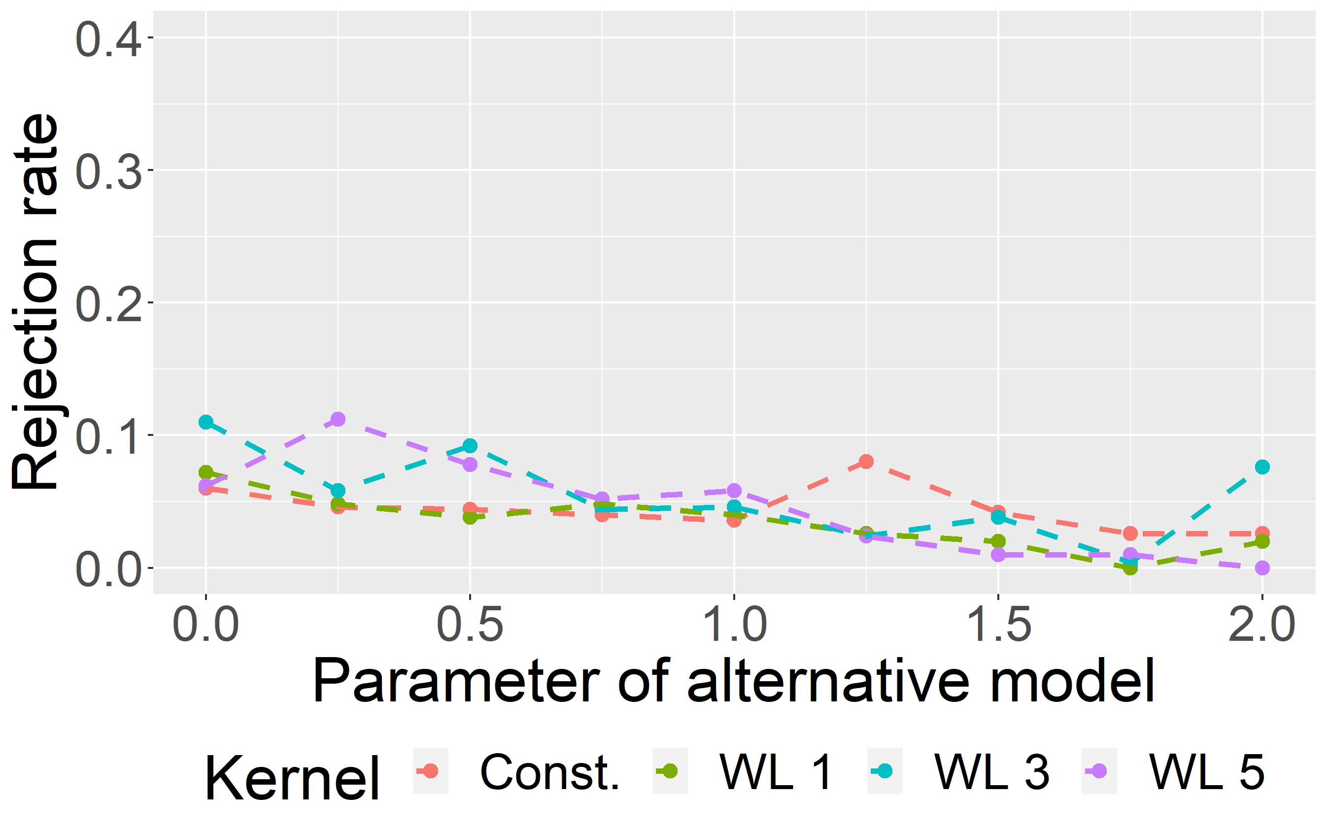
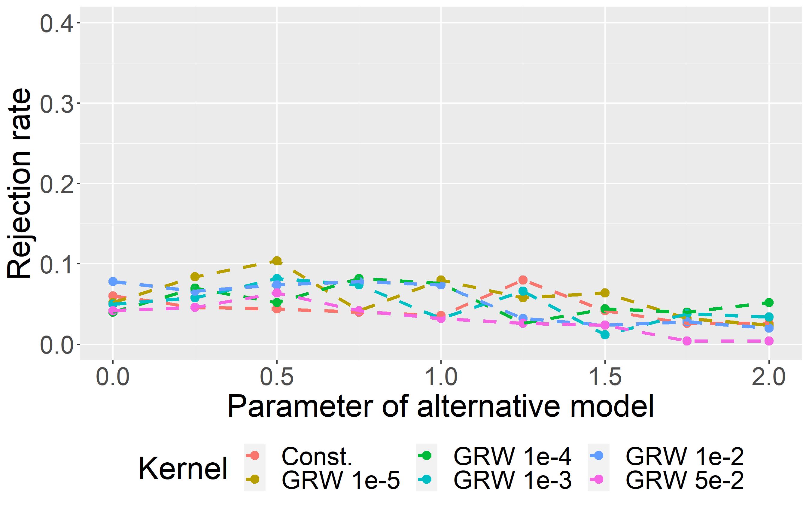
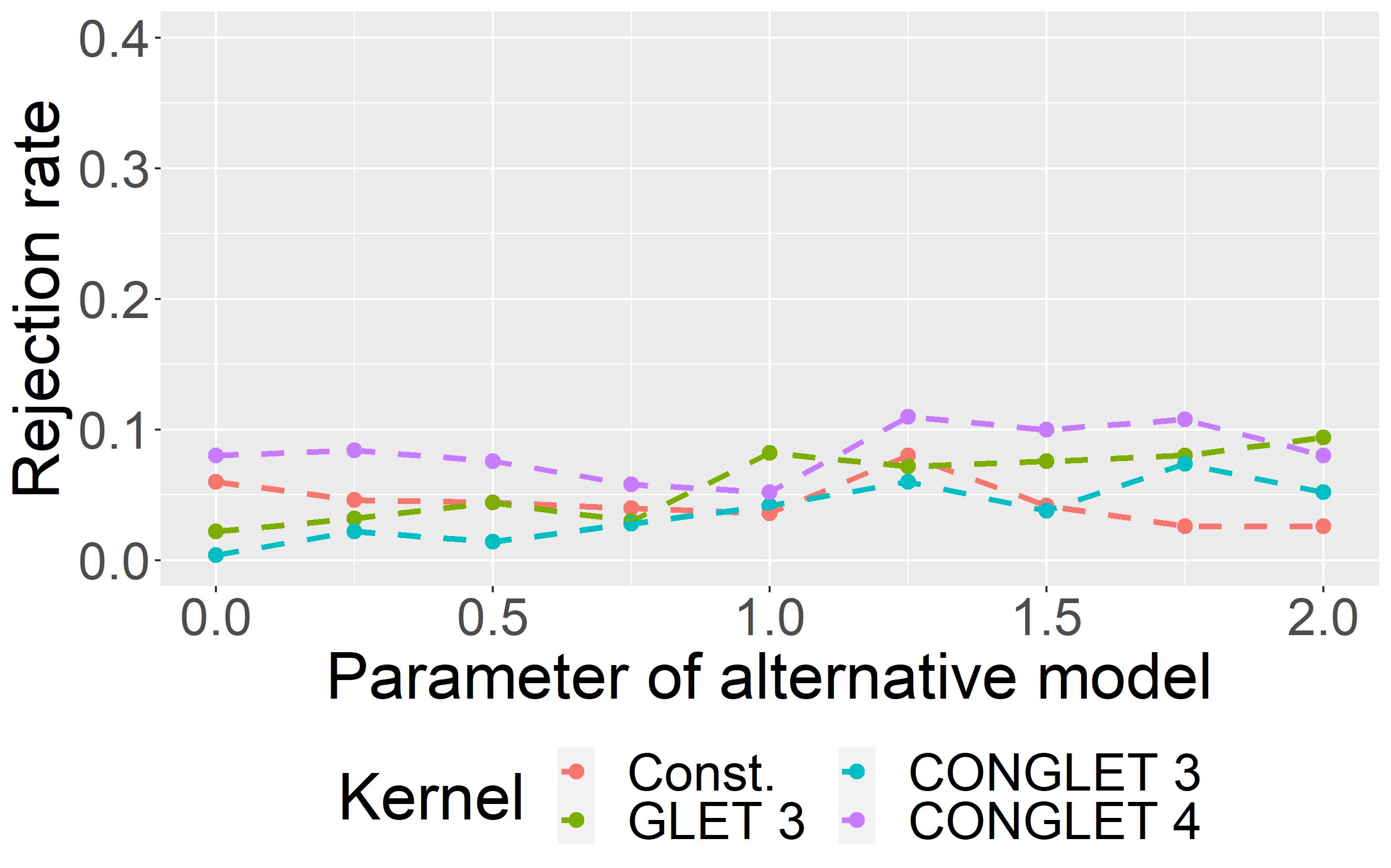
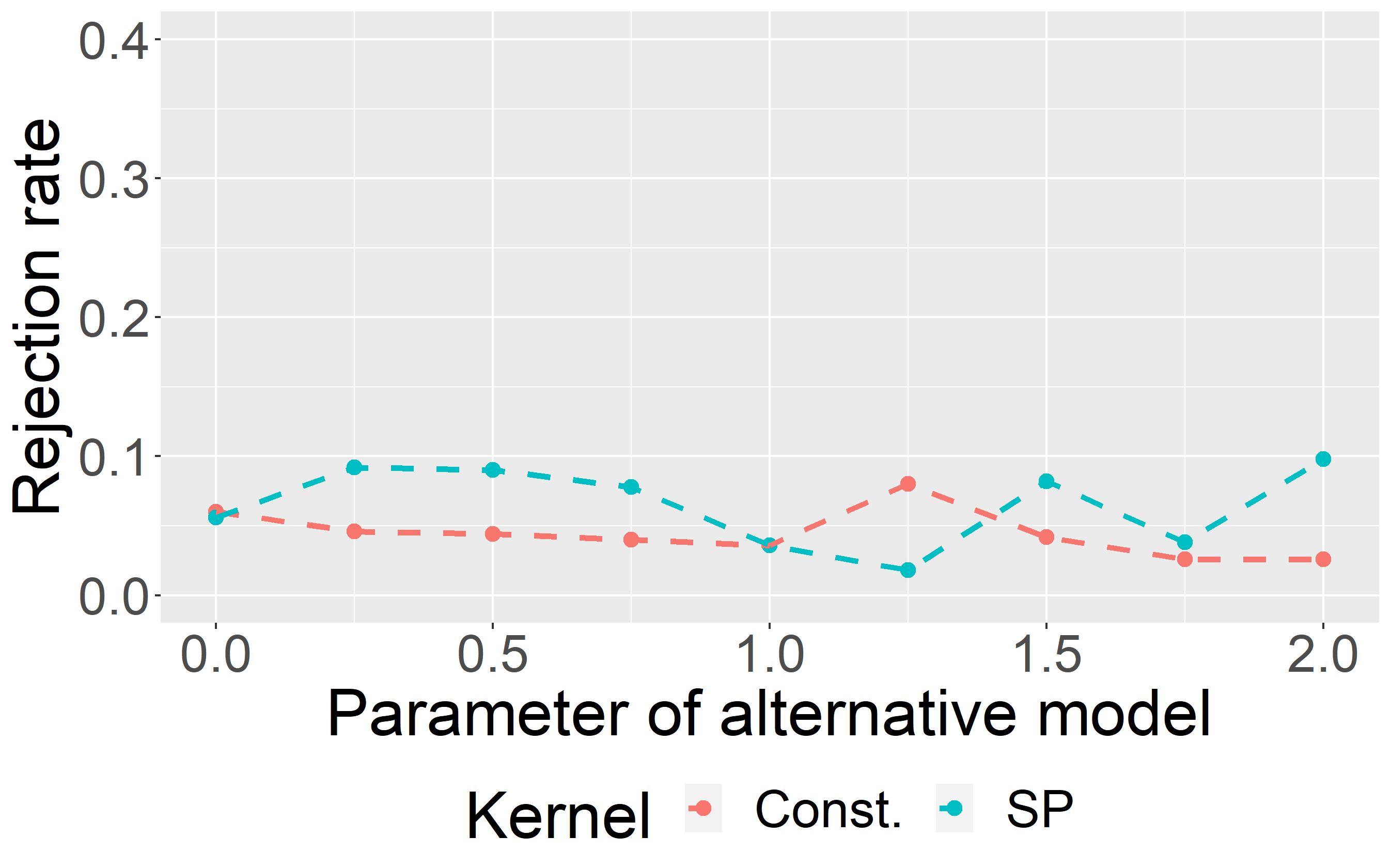
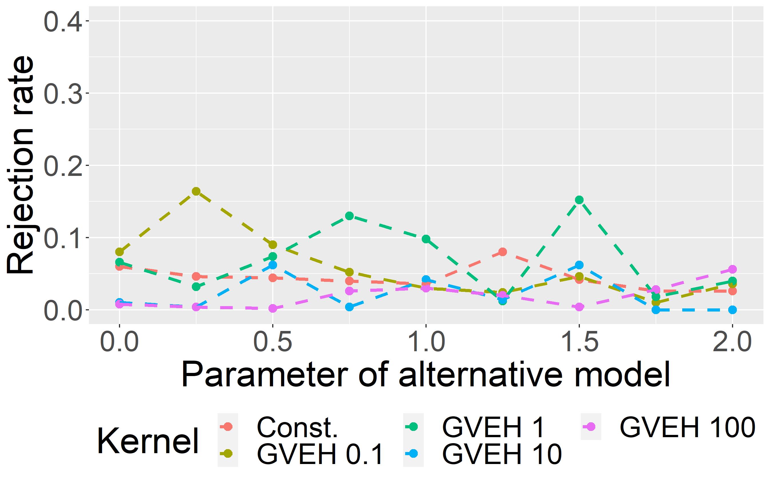
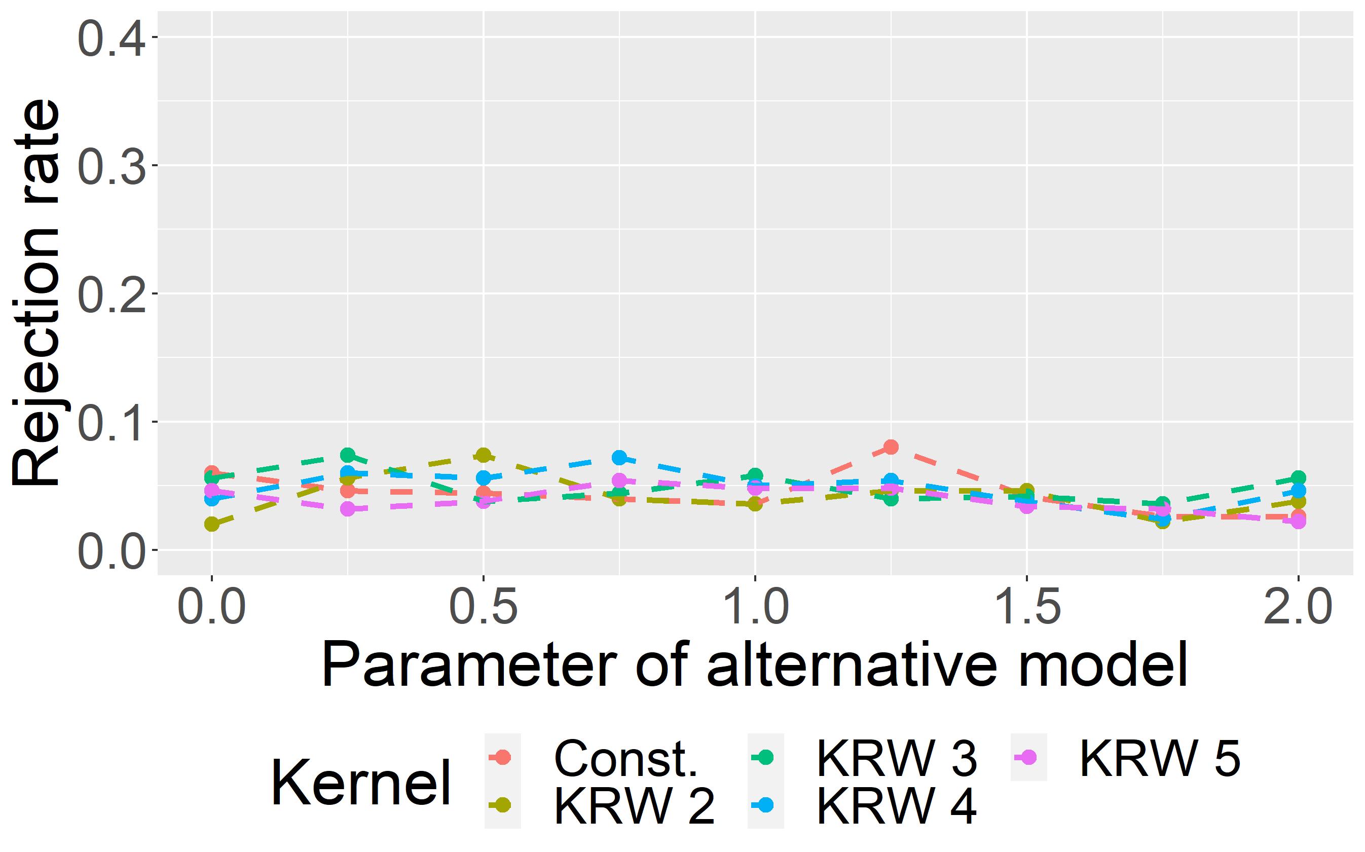
Figure 12: AgraSSt for BA model with $m=1$; $t(x)$ being the edge density.

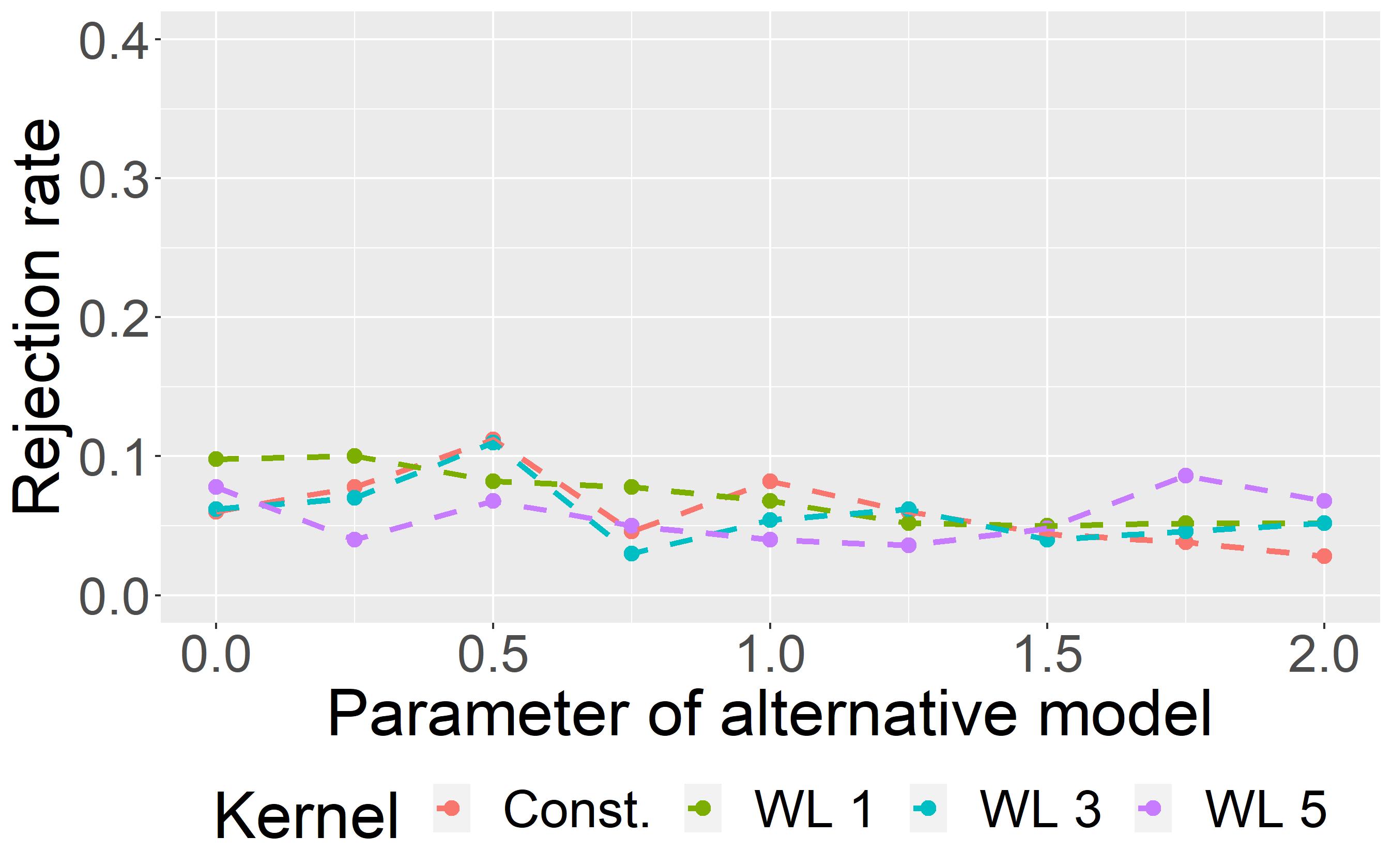
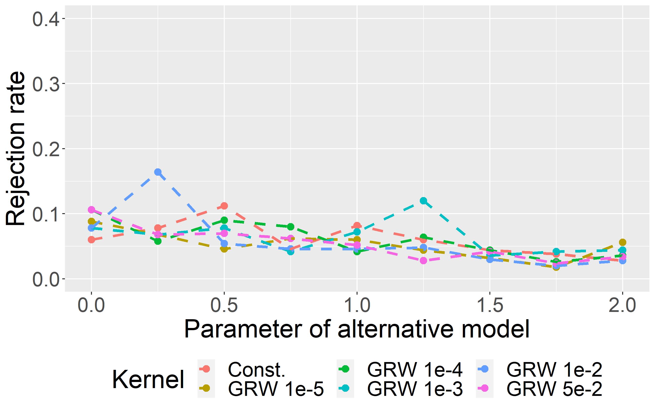
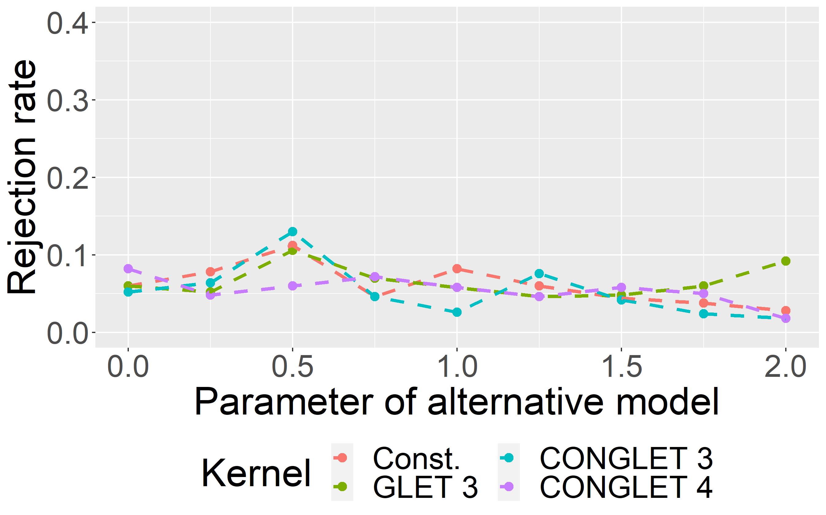
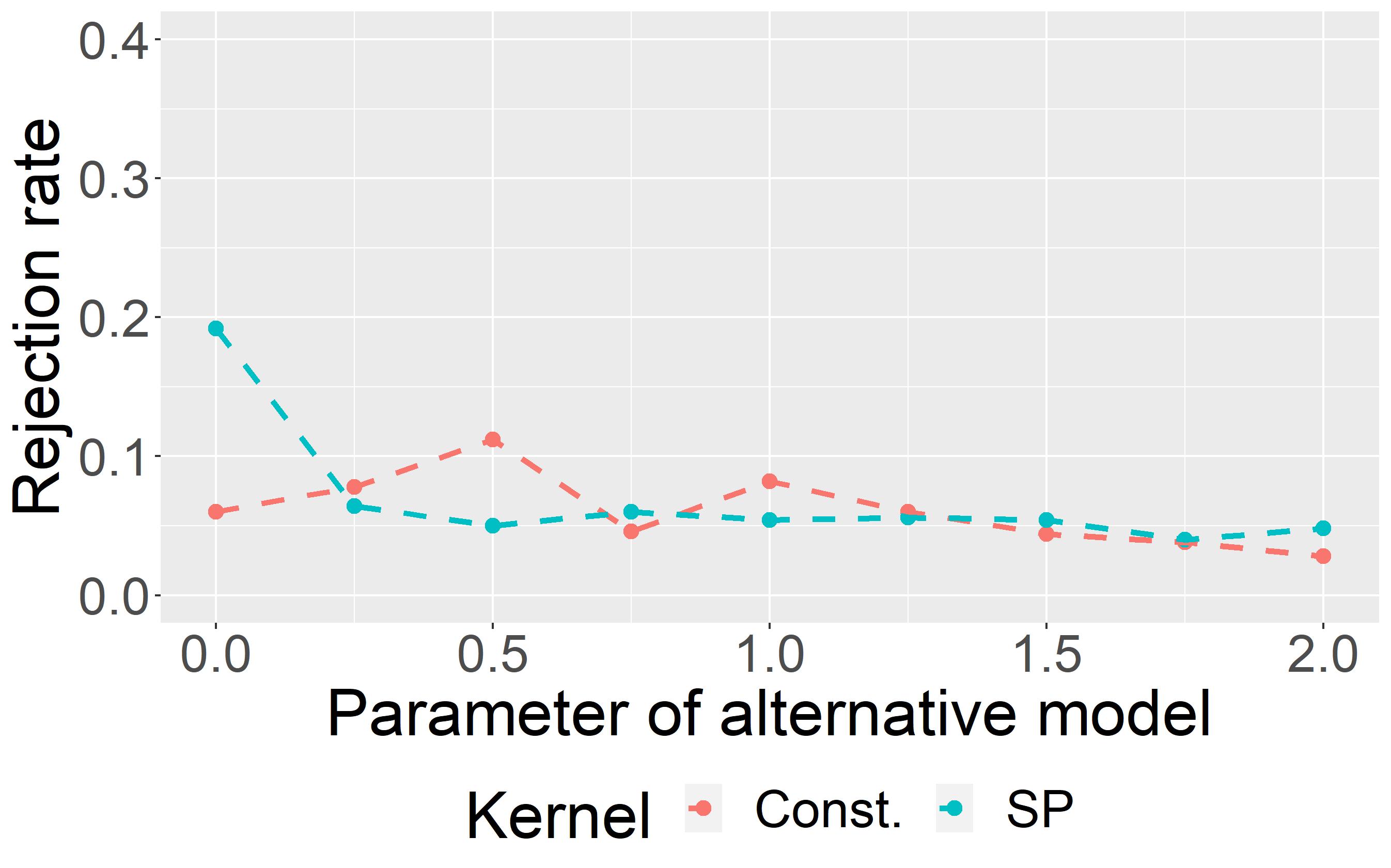
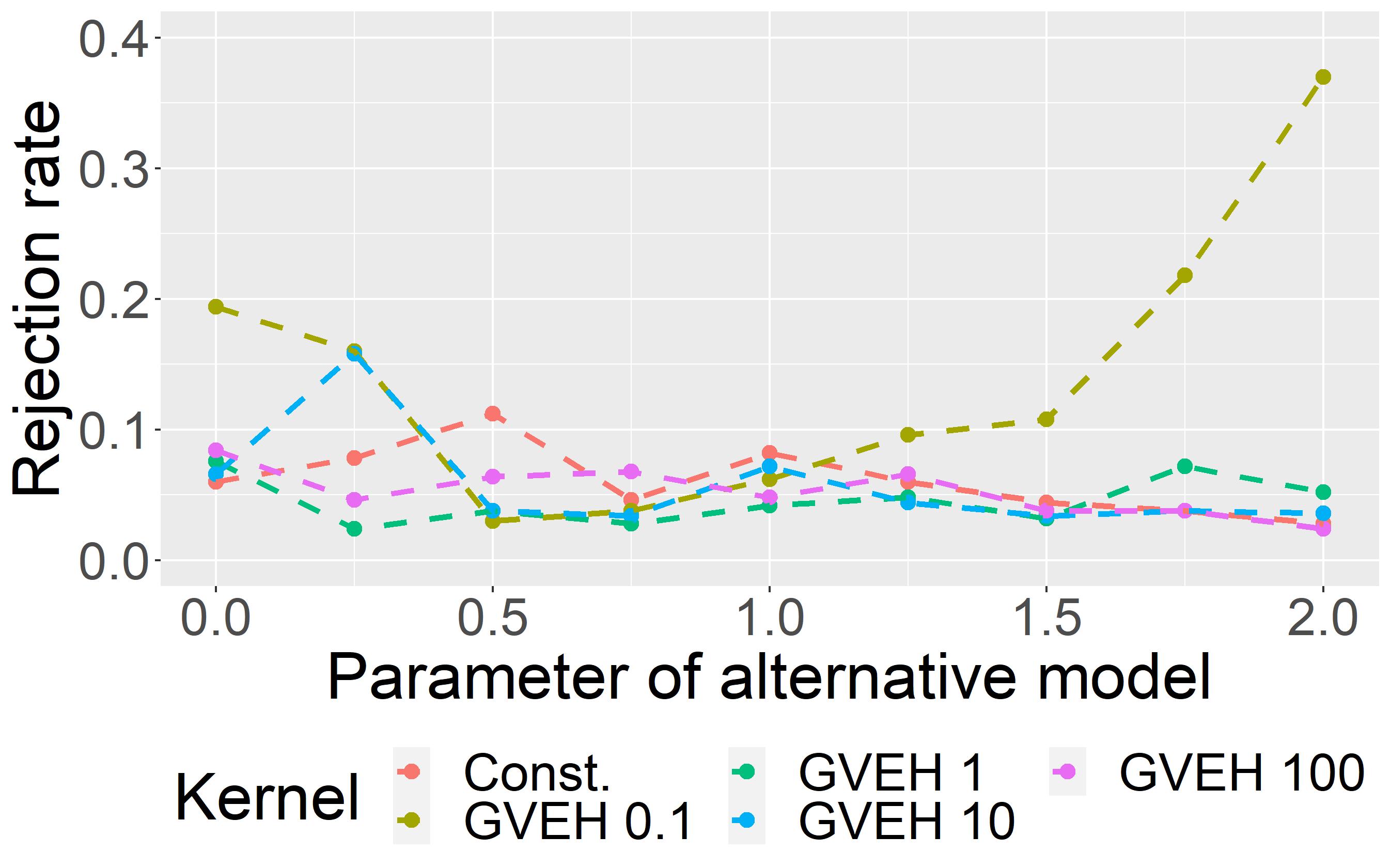
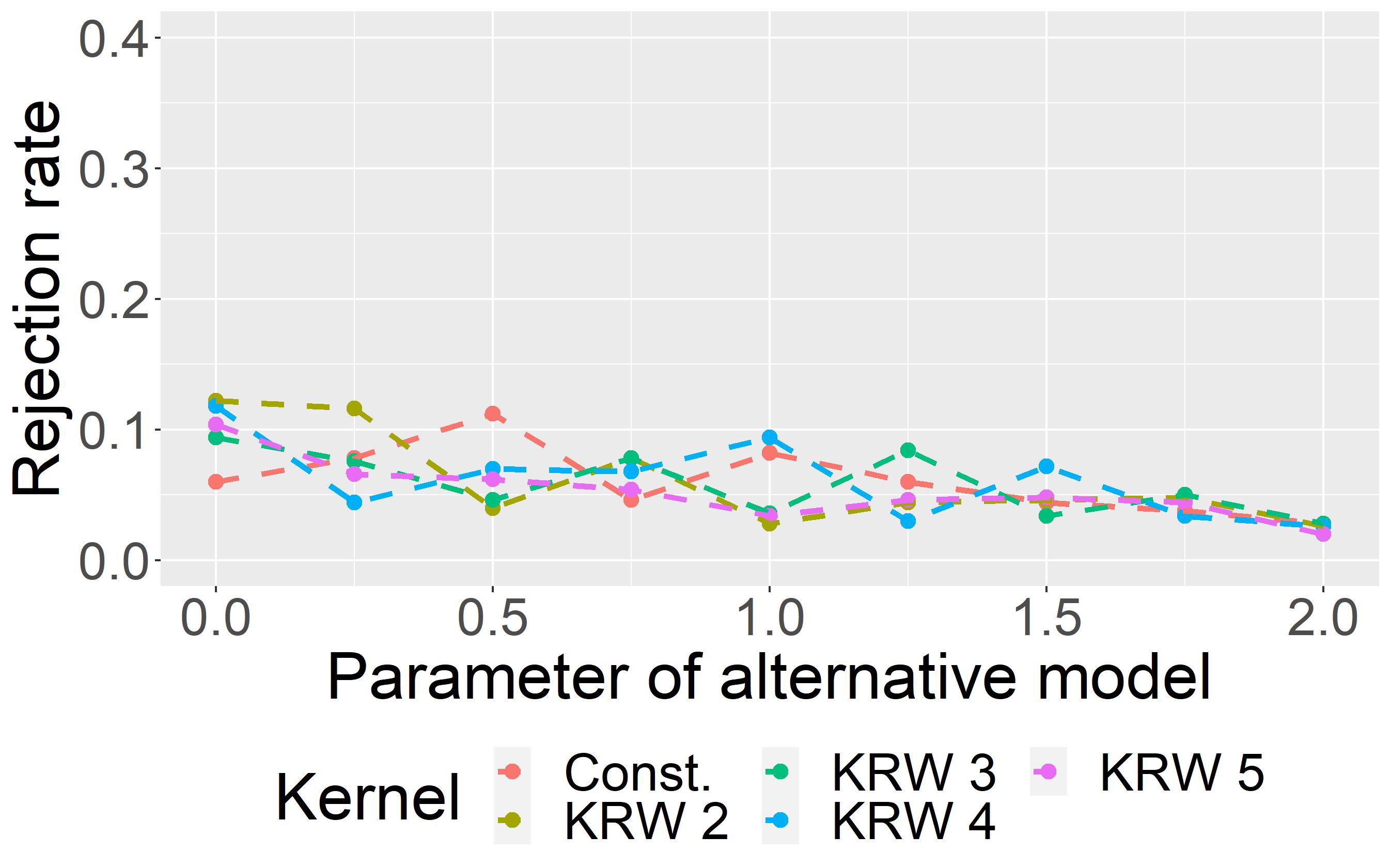
Figure 13: AgraSSt for BA model with $m=1$; $t(x)$ being the bivariate degree vector.

A Barabasi-Albert model generates scale-free networks using preferential attachment. The algorithm starts with a complete graph of $m$ vertices, where $m\in\mathbb{N}$ is chosen as a parameter of the model. In every step, one vertex is added and connected with $m$ edges to the network. The version used here is from the R package igraph; the probability of a vertex $v$ being chosen to connect to the new vertex depends on its current degree via

$$p_{v}\propto deg(v)^{\alpha}+1,$$

where $\alpha$ is a power parameter which governs the intensity of preference for high-degree vertices in the attachment step. When $m\geq 2$ the degrees are updated after the first edge is added and before the second edge is added, and the second edge is then added according to the updated degrees. If $\alpha=0$, the vertices to attach to are chosen uniformly at random, whereas $\alpha=2$ leads to graphs which are almost starlike with one central vertex (or for $m>1$ multiple central vertices) and most of the remaining vertices only connected to the centre. For $\alpha>0$ vertices with higher degree are more likely to connect to new vertices, leading to few vertices with unusually high degrees in comparison to other graph generators. Unlike in ERGMs or GRG models, a change of the parameter $\alpha$ does not result in a change of edge density.

We carry out tests of the form $M0:\operatorname{BA}\alpha_{M0}=1$ versus $M1:\operatorname{BA}\alpha_{M1}$, with $\alpha_{M1}$ ranging from $0$ to $2$. The rejection rates for $m=1$ are shown in Figure 12 and Figure 13. Furthermore, the results of the experiment for $m=2$ are shown in Figure 14 and Figure 15. We note that here a change in the parameter, $\alpha$, does not generally yield high rejection rates. This is not surprising for $t(x)$ the edge density, as edge density is not influenced by $\alpha$, but for most kernels this also the case for $t(x)$ the bivariate degree vector. For $m=1$ notable exception is the Gaussian vertex-edge histogram kernel with small parameter $\sigma=0.1$. This kernel is tailored to assessing degree pairs and hence it is plausible that it picks up the power law distribution in the degrees. In this example the choice of kernel and of parameter can make a considerable difference. For $m=2$ also the GRW kernel with $\lambda=0.5$ and the WL kernel with level $3$ and $5$ pick up some signal.

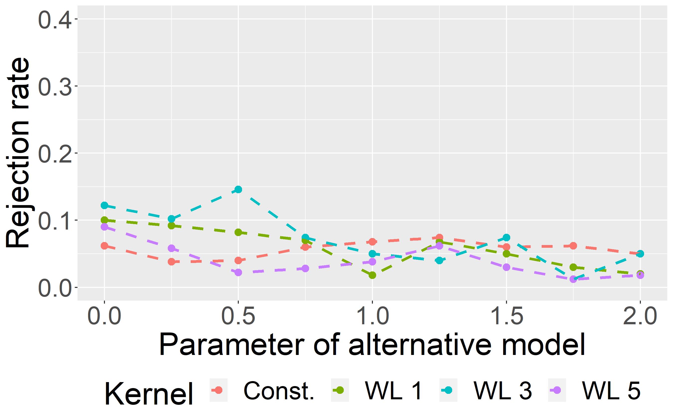
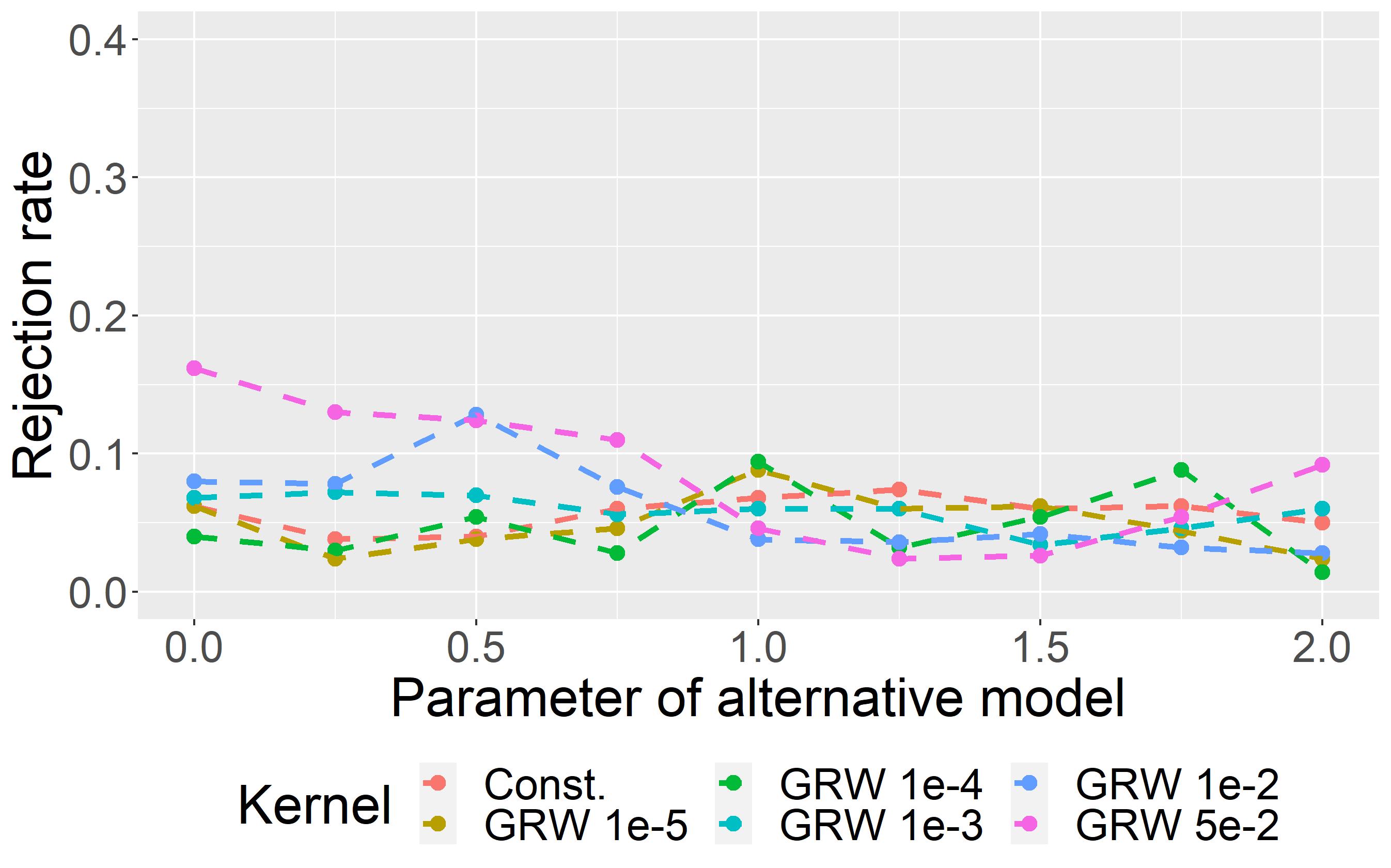
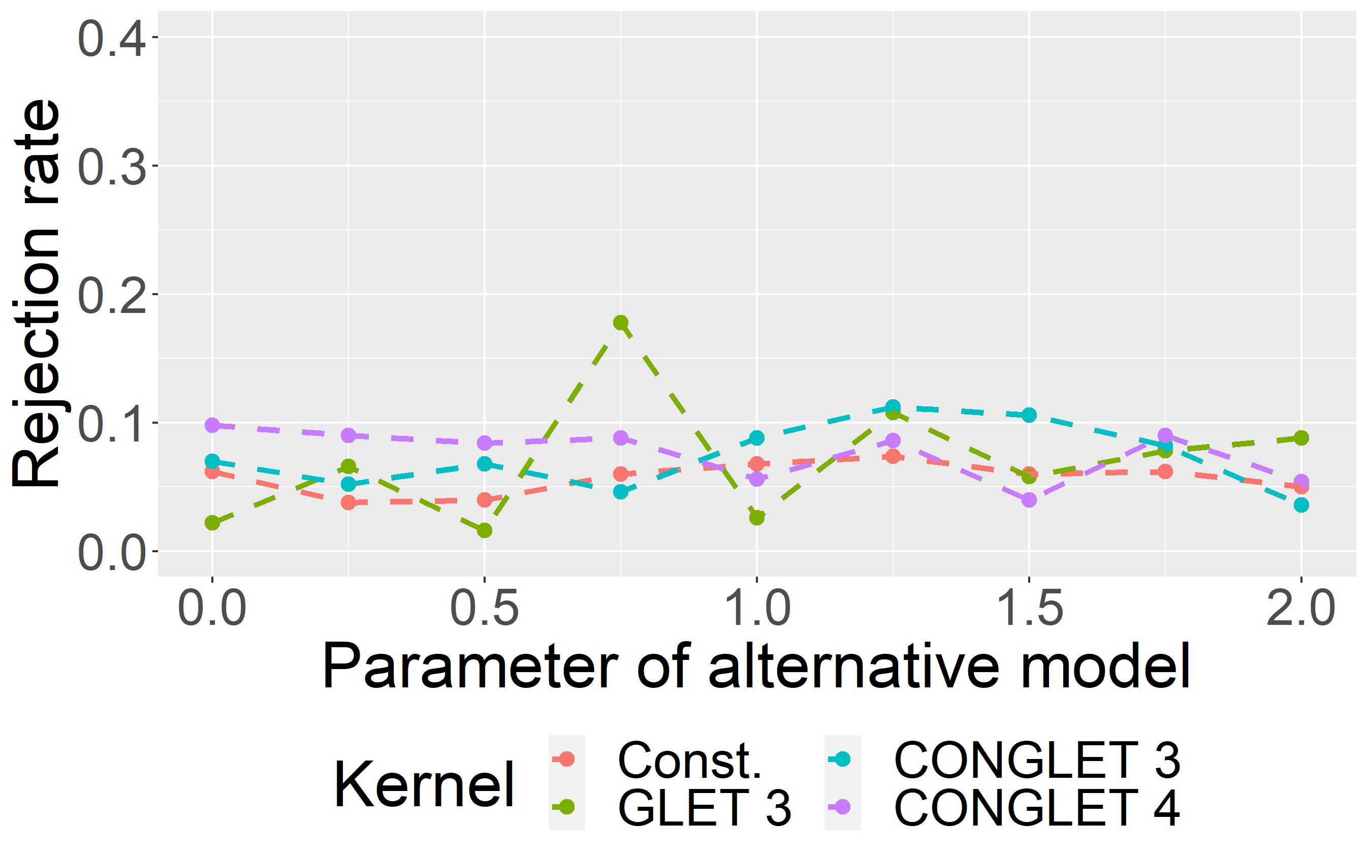
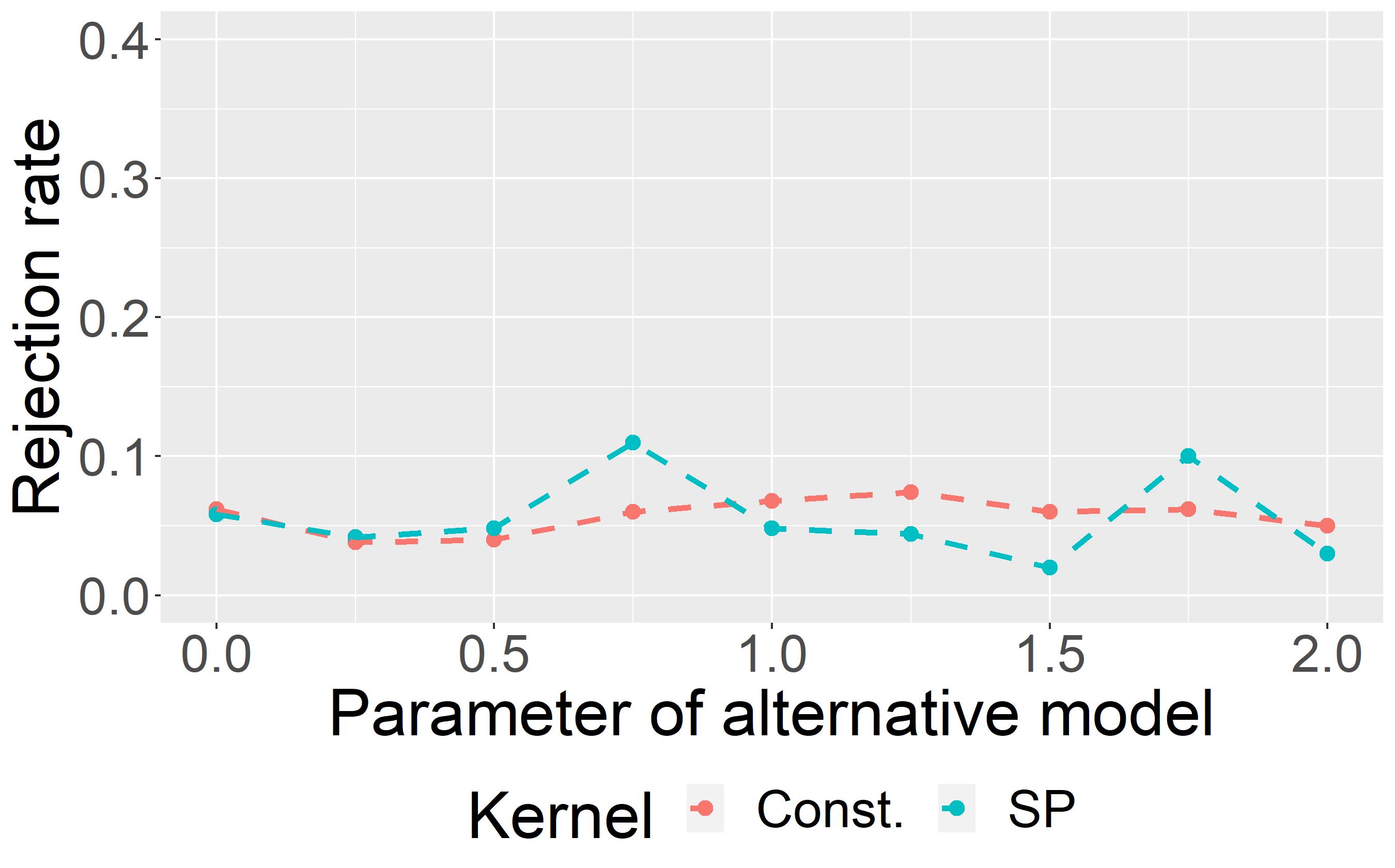
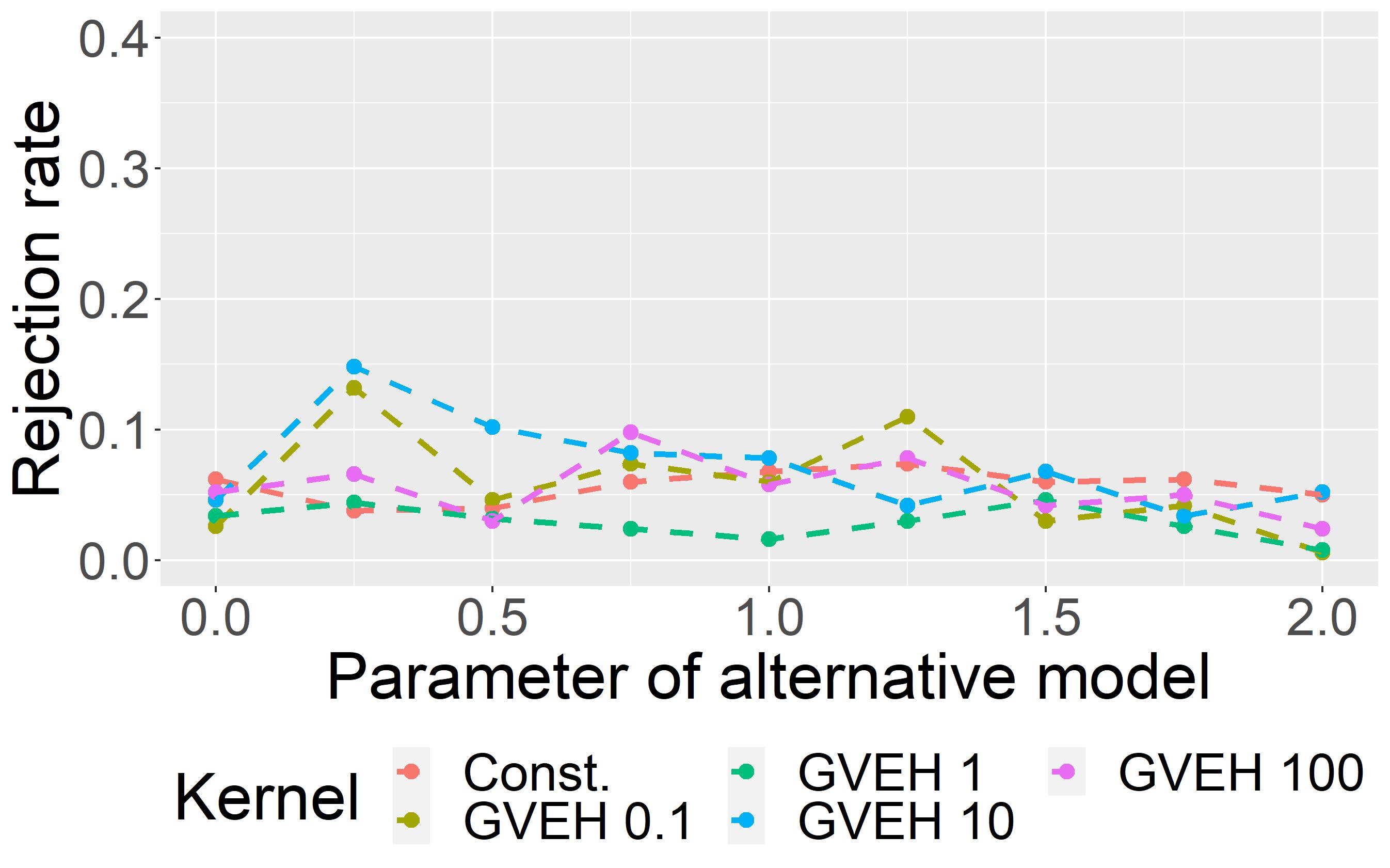
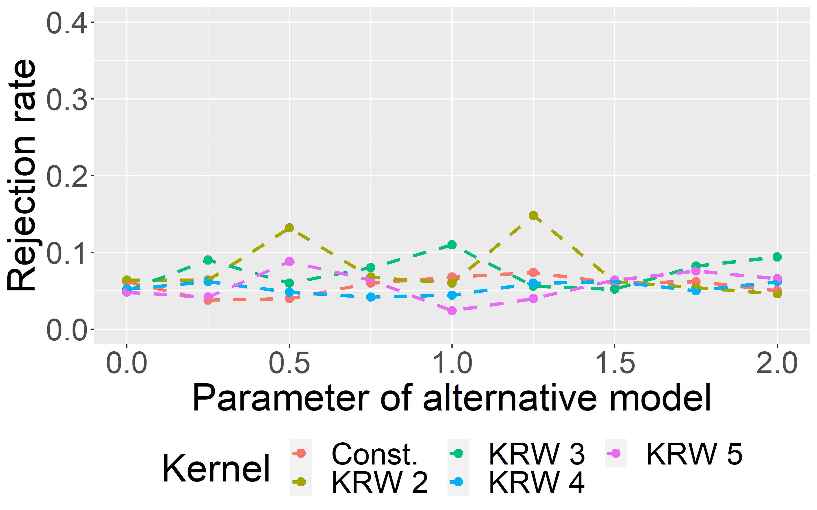
Figure 14: AgraSSt for BA model with $m=2$; $t(x)$ being the edge density.

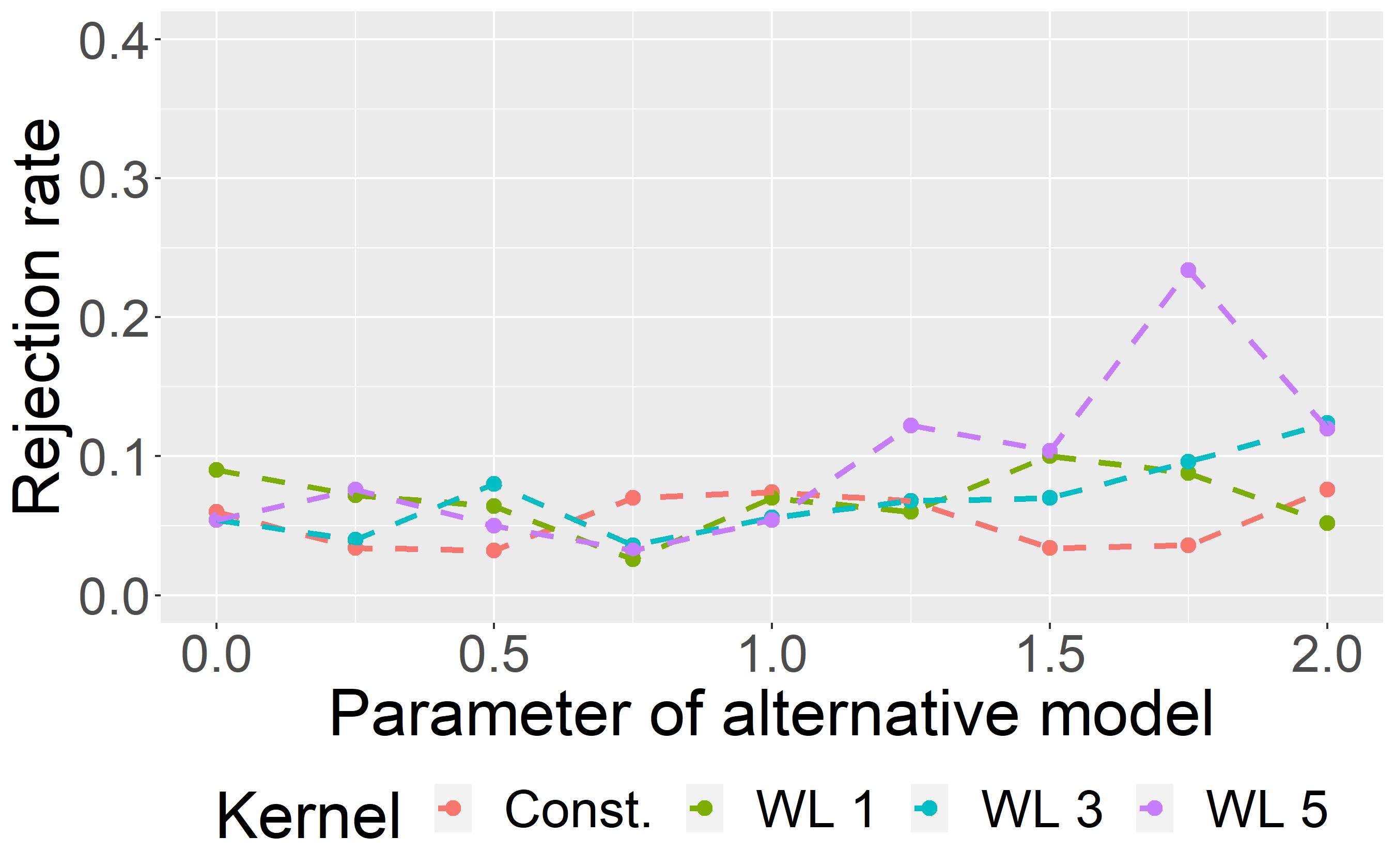
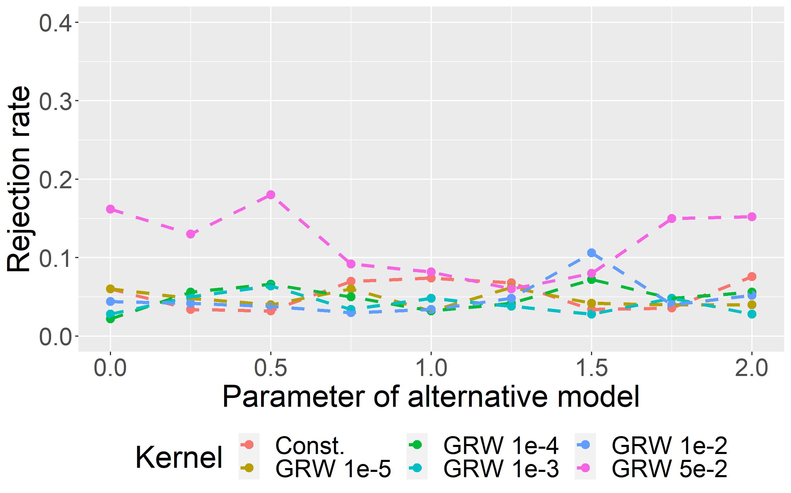
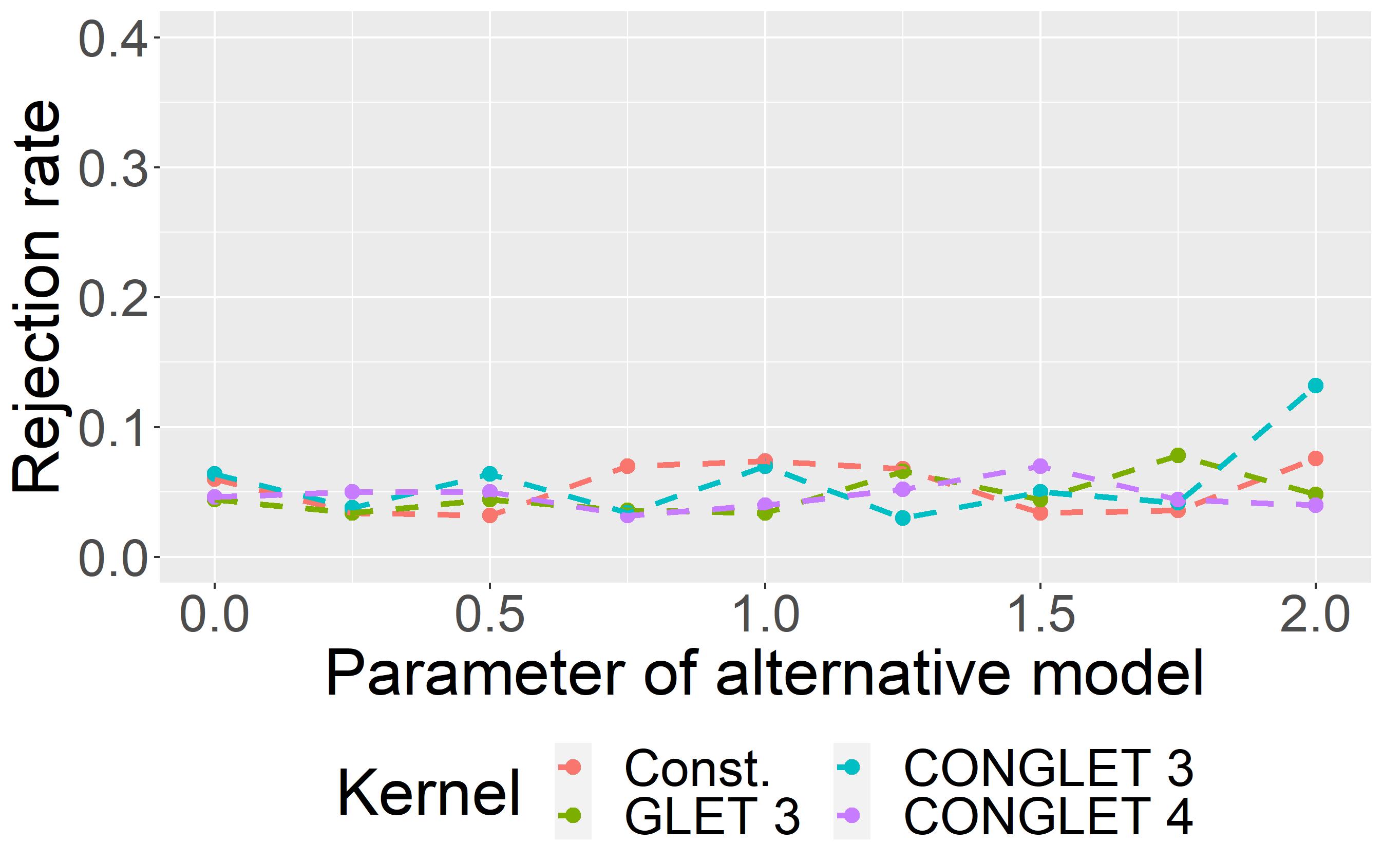
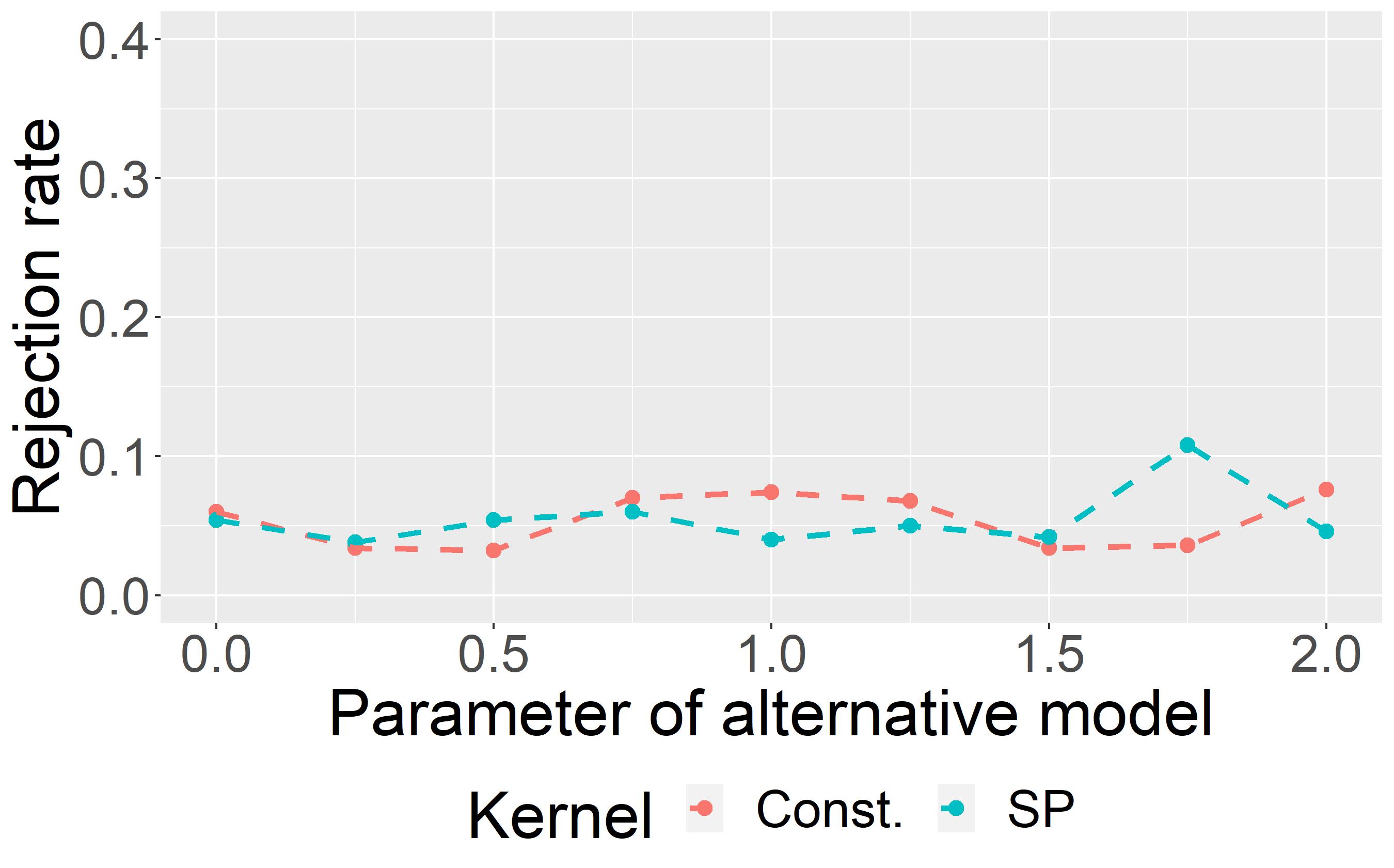
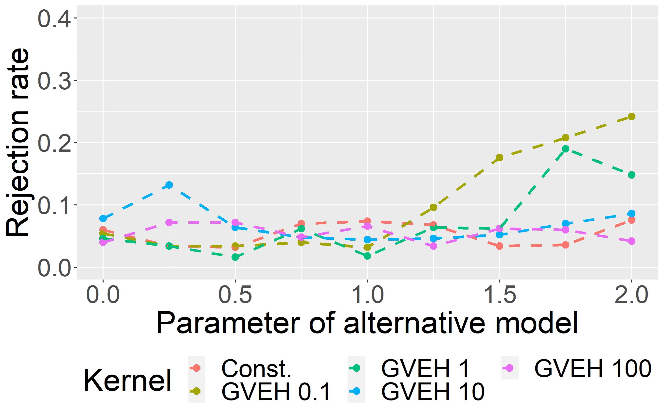
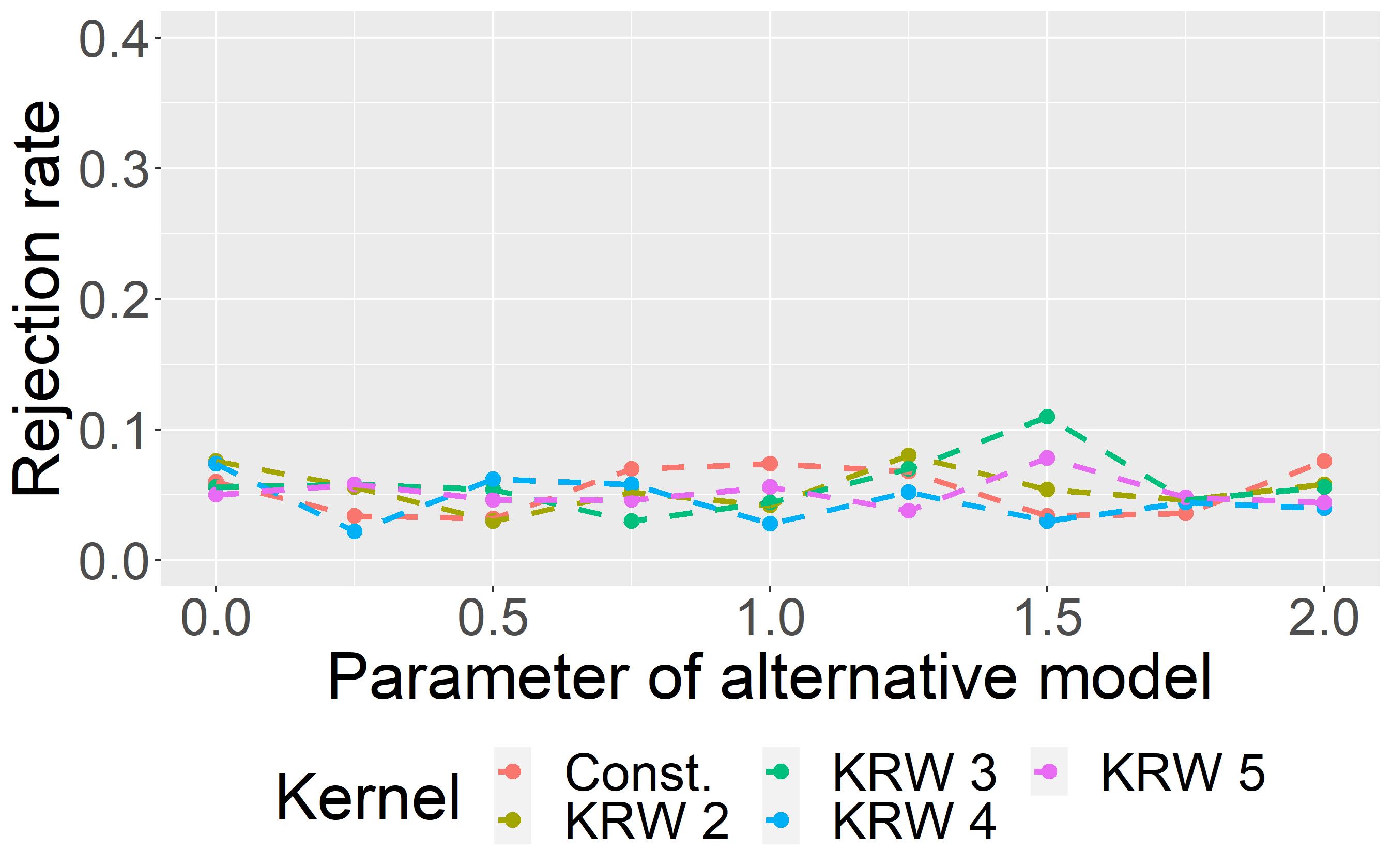
Figure 15: AgraSSt for BA model with $m=2$; $t(x)$ being the bivariate degree vector.

B.3 Additional CELL experiments

B.3.1 Synthetic data

For our additional experiments we first choose a theoretical graph generator as null model $M0$. By the construction of CELL, the generator can only be trained on a single network and by repeating the training process, we reduce the risk of sampling an unrepresentative network from $M0$ and thus making all networks trained on this generator unrepresentative.

For all samples from ${M1}$, we perform a Monte Carlo test based on sampled AgraSSt with different statistics $t$. In the case of the E2S-model which is a ERGM and hence gKSS is applicable, we additionally compare to sampled gKSS, to obtain average rejection rates for different graph kernels $k$. As null model, we test the E2S-model with parameters $\beta=(-2,0)$, the Geometric Random Graph model with radius $r=0.3$ on a unit square without torus structure, and the Barabasi-Albert model with $m=1$ and power parameter $\alpha=1$.

An E2ST experiment

Rejection rates for the E2S-model are displayed in Table 2. We observe that rejection rates for all statistics and kernels are around 5%, which is expected if the CELL-simulated samples are not distinguishable from the original graph generator. The two-star coefficient of our null model is $\beta_{2S}=0$, hence the only criterion of a graph affecting the probability distribution of the model is its edge density. As the CELL-simulated graphs have the same edge density as the graph the generator was trained on, we may expect the alternative model to get rejected in roughly 5% of cases. We note that gKSS, which for this model includes edges and two-stars as sufficient statistics, has only slightly lower rejection rates on average than AgraSSt.

Kernel	gKSS	Avg. density	Bidegree statistic	Common neighbour statistic
Const.	0.02	0.04	0.05	0.05
GVEH 0.1	0.04	0.07	0.09	0.07
GVEH 1	0.03	0.04	0.05	0.05
GVEH 10	0.01	0.04	0.02	0.06
GVEH 100	0.04	0.04	0.02	0.06
SP	0.06	0.05	0.05	0.05
KRW 2	0.02	0.03	0.01	0.05
KRW 3	0.04	0.03	0.05	0.05
KRW 4	0.02	0.04	0.04	0.05
KRW 5	0.02	0.04	0.03	0.05
GRW 1e-5	0.05	0.03	0.03	0.05
GRW 1e-4	0.03	0.02	0.04	0.06
GRW 1e-3	0.03	0.02	0.04	0.06
GRW 1e-2	0.02	0.05	0.03	0.05
GRW 5e-2	0.02	0.04	0.03	0.05
WL 1	0.03	0.04	0.03	0.05
WL 3	0.03	0.04	0.06	0.03
WL 5	0.04	0.04	0.05	0.04
GLET 3	0.02	0.02	0.03	0.06
CONGLET 3	0.02	0.03	0.05	0.05
CONGLET 4	0.04	0.02	0.02	0.04

Table 2: Rejection rates for CELL-simulated Edge-Two star graph samples with parameters $\beta=(-2,0)$ using the gKSS and AgraSSt testing procedure with different summary statistics. Rejection rates over 5% are marked in amber, and rejection rates of at least 10% would have been marked in red.

The geometric random graph experiment

Table 3 shows the rejection rates in the Geometric Random Graph experiment from Section 4, now using CELL. The rates for AgraSSt based on the average density are all roughly 5%. While this statistic is effective at distinguishing between different radius parameters in the experiment with the Geometric Random Graph model in Section 4, this may just reflect that a change in radius also changes the average edge density. When using the bidegree statistics the average rejection rate is slightly higher than 5% and some kernels achieve a rejection rate of over 10%. Only some of the Weisfeiler-Lehman kernels achieve at most 5% rejection rate, under the bidegree statistic.

The common neighbour statistic achieves the highest rejection rates as all but one kernel reject in 10% or more of cases. The maximal rejection rate of 16% is achieved by the Gaussian vertex-edge histogram Kernel with bandwidth $\sigma=0.1$, the Shortest Path kernel and the Geometric Random Walk kernel with weight $\lambda=0.01$. These results align with our findings in Section 4 where the common neighbour statistic achieved higher rejection rates than the bidegree statistic and the Gaussian vertex-edge Histogram kernel achieved the best results. In analysing the graphs which are rejected by the Shortest Path kernel, we can furthermore see that CELL has a tendency to connect small disconnected components to the rest of the graph and create additional paths between components which are only attached through one edge (see Figure 16). So it appears that CELL may struggle with generating networks which are constituted by a few disconnected or sparsely connected components. However, the case of many disconnected components, as generated by the sparse E2S-model, seems unproblematic. Altogether however, rejection rates remain fairly low for all kernels, indicating that CELL produces fairly accurate samples despite its flaws.

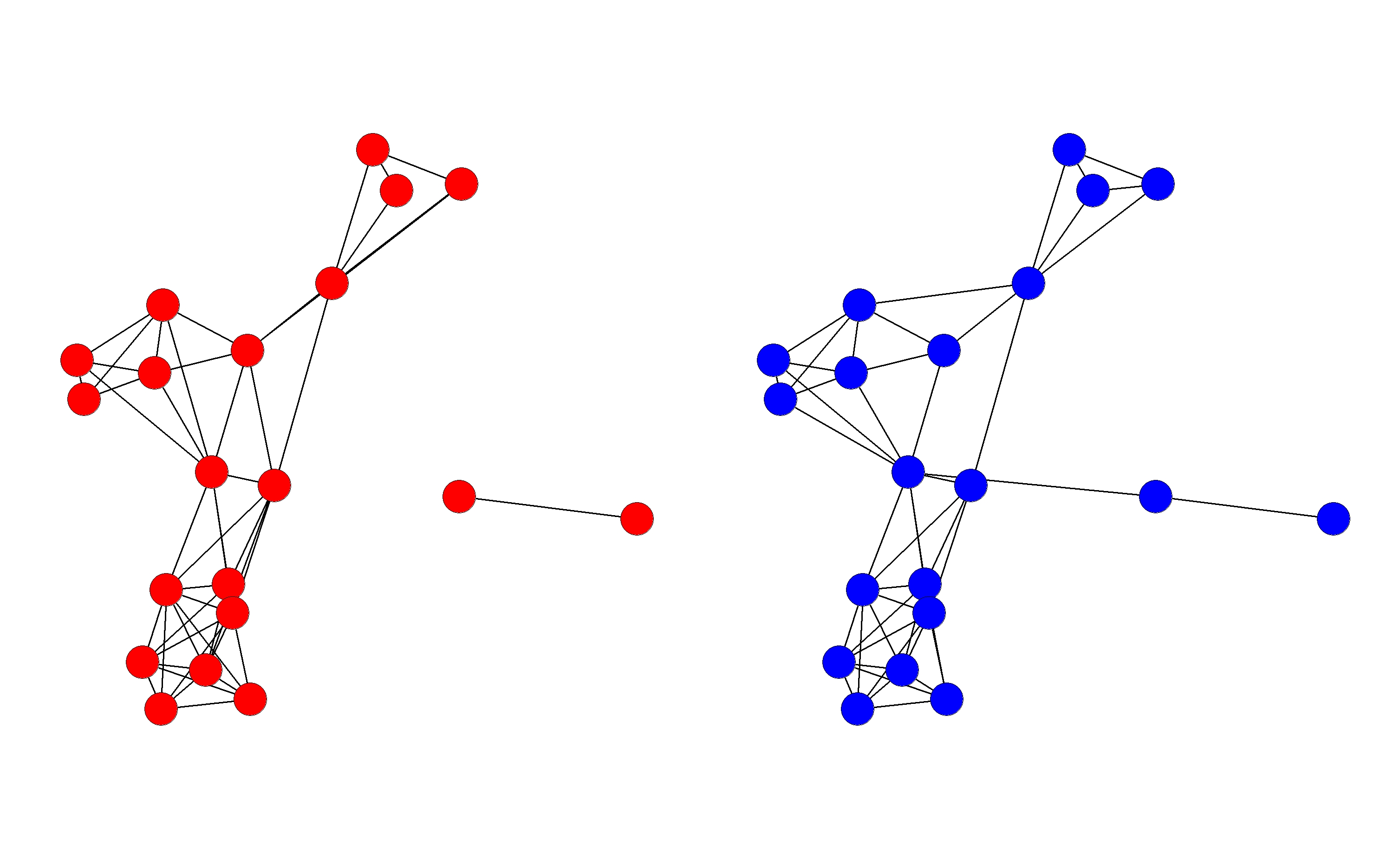
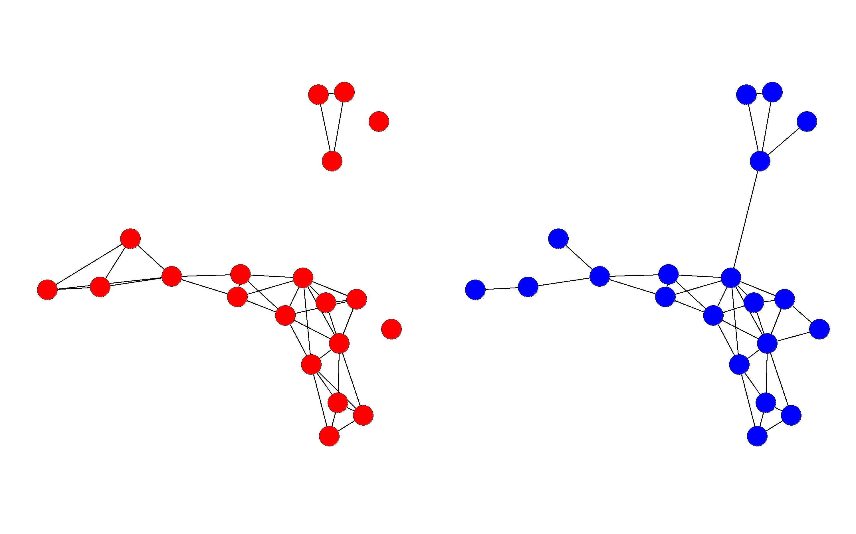
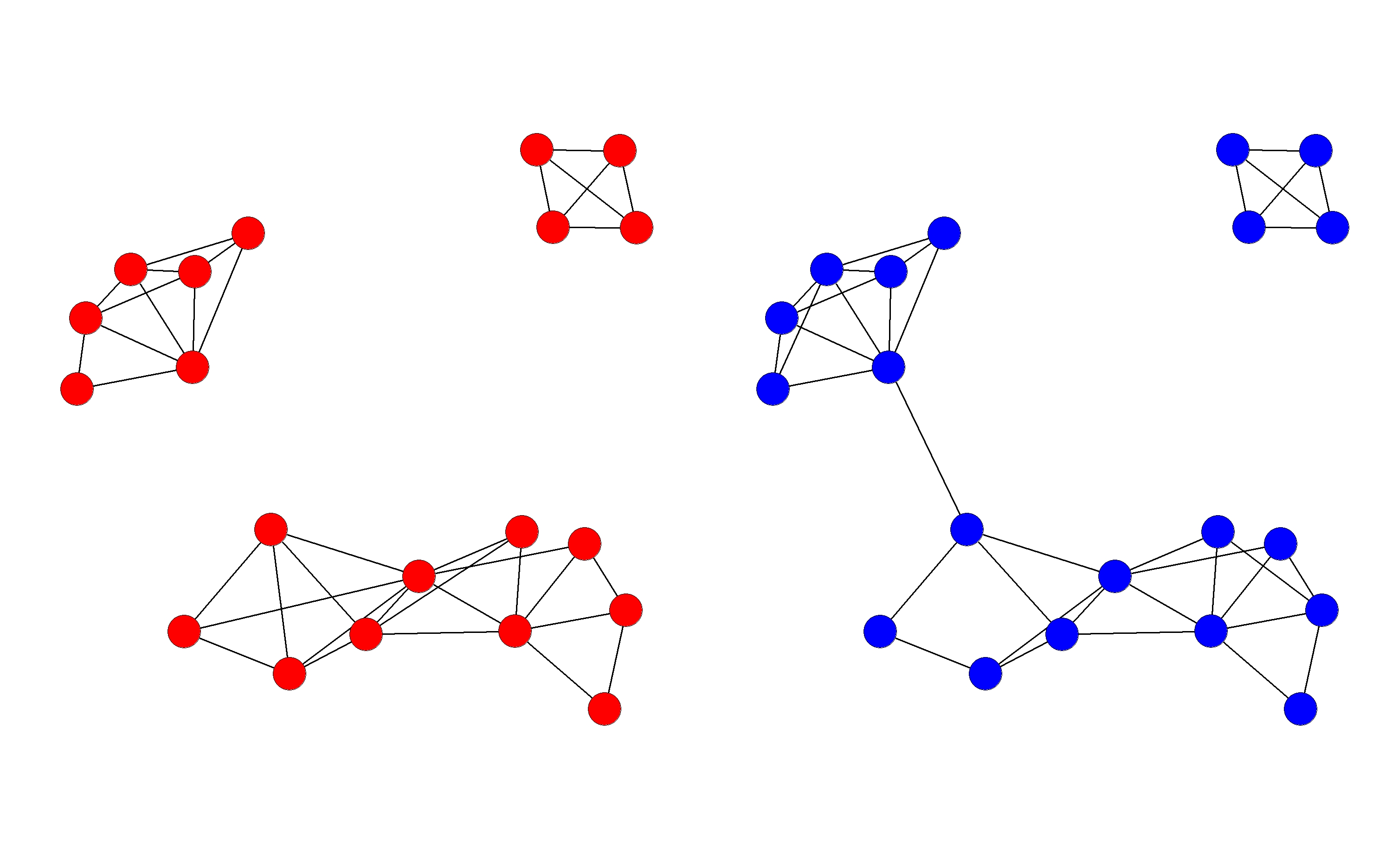
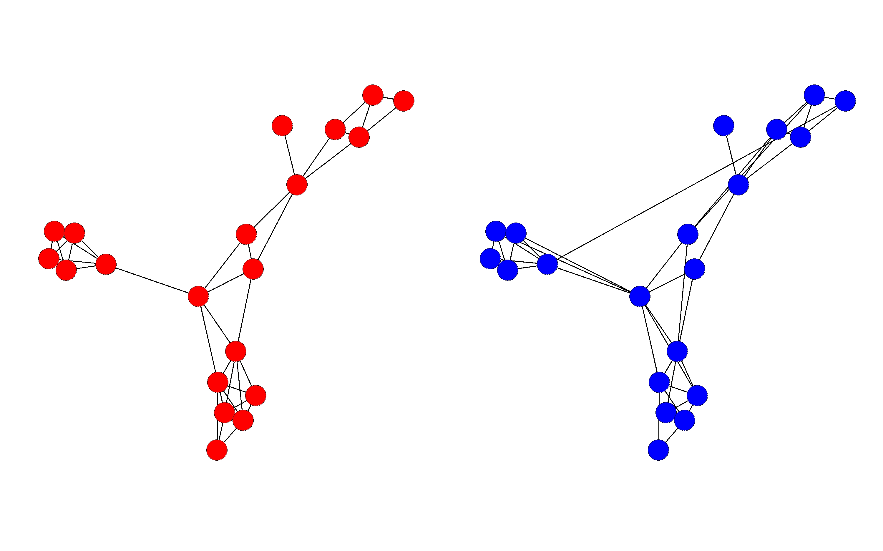
Figure 16: CELL-samples for the Geometric Random Graph model: original network is displayed in red, and the CELL sample is displayed in blue.

Kernel	Avg. density	Bidegree statistic	Common neighbour statistic
Const.	0.03	0.09	0.12
GVEH 0.1	0.08	0.08	0.16
GVEH 1	0.09	0.08	0.11
GVEH 10	0.04	0.13	0.12
GVEH 100	0.03	0.09	0.07
SP	0.06	0.09	0.16
KRW 2	0.03	0.10	0.12
KRW 3	0.07	0.09	0.15
KRW 4	0.08	0.10	0.12
KRW 5	0.04	0.06	0.15
GRW 1e-5	0.04	0.07	0.10
GRW 1e-4	0.02	0.08	0.15
GRW 1e-3	0.05	0.10	0.16
GRW 1e-2	0.06	0.07	0.12
GRW 5e-2	0.03	0.08	0.09
WL 1	0.06	0.08	0.14
WL 3	0.04	0.04	0.10
WL 5	0.04	0.05	0.15
GLET 3	0.04	0.08	0.14
CONGLET 3	0.04	0.08	0.15
CONGLET 4	0.03	0.10	0.10

Table 3: Rejection rates for CELL-simulated Geometric Random Graph samples with parameters $r=0.3$ on a unit-square without torus structure using the AgraSSt testing procedure with different summary statistics. Rejection rates over 5% are marked in amber, and rejection rates of at least 10% are marked in red.

The Barabasi-Albert experiment

Rejection rates for the Barabasi-Albert model, now using CELL, with parameters $m=1$ and $\alpha=1$ are presented in Table 4. We observe that while their average lies slightly above 5%, samples from CELL would be still accepted at the 10% level in the majority of cases. AgraSSt with the bidegree statistic achieves the largest rejection rates, which agrees with our findings in Section B.2. Similarly, the Gaussian vertex-edge histogram kernel achieves the highest rejection rate with a maximum of 16% with bandwidth $\sigma=1$. The Weisfeiler-Lehman kernel also performs well, attaining a rejection rate of 13% for any level parameter and a maximum of 16% for $h=3$. While the Weisfeiler-Lehman kernel was not effective in distinguishing between different power parameters $\alpha$ for $m=1$, it did boost the rejection rates of sampled AgraSSt with the bidegree statistic for $m=2$ Out of the 100 simulated samples, 58 graphs contain multiple disconnected subgraphs or cycles, which should make them clearly distinguishable from graphs created by the Barabasi-Albert model with $m=1$, whereas only 42 are connected and contain no cycle. Most kernels do a good job at accepting connected graphs, above all the connected graphlet kernel of size 4. Out of the 10 graphs it rejects, only one is connected, and the other 41 connected graphs are accepted by the testing procedure. However, all kernels still accept a large number of disconnected networks.

Kernel	Avg. density	Bidegree statistic	Common neighbour statistic
Const.	0.07	0.05	0.10
GVEH 0.1	0.08	0.13	0.05
GVEH 1	0.06	0.16	0.05
GVEH 10	0.04	0.09	0.09
GVEH 100	0.07	0.08	0.08
SP	0.05	0.07	0.08
KRW 2	0.07	0.08	0.07
KRW 3	0.10	0.10	0.12
KRW 4	0.08	0.06	0.09
KRW 5	0.07	0.08	0.10
GRW 1e-5	0.09	0.09	0.12
GRW 1e-4	0.07	0.07	0.09
GRW 1e-3	0.04	0.08	0.09
GRW 1e-2	0.04	0.12	0.09
GRW 5e-2	0.08	0.08	0.08
WL 1	0.09	0.13	0.04
WL 3	0.08	0.16	0.05
WL 5	0.07	0.13	0.08
GLET 3	0.10	0.11	0.08
CONGLET 3	0.07	0.08	0.09
CONGLET 4	0.10	0.10	0.07

Table 4: Rejection rates for CELL-simulated Barabasi-Albert graph samples with parameters $m=1$ and $\alpha=1$ using the AgraSSt testing procedure with different summary statistics. Rejection rates over 5% are marked in amber, and of at least 10% are marked in red.

B.3.2 Details on the Karate club network and the CELL results

Zachary’s Karate Club network Zachary, (1977) contains 34 vertices, representing the members of a university sport society before its separation into two new groups due to a conflict between the instructor and the administrator. An edge in the network symbolizes consistent interaction between members outside of karate classes. Using the structural information about friendships in the club, Zachary found a method to cluster the vertices which for all but one member agreed with the side they would end up after the split. The network became a widespread example of community structures after its use by Girvan and Newman, (2002).

We perform a Monte Carlo test, in which we compare sampled AgraSSt with sample size $B=200$ of the original network to $n_{M1}=100$ simulations from CELL and reject at the 5%-level. This procedure is repeated 100 times to obtain average rejection rates. The complete results are displayed in Table 5. Most rejection rates remain at around 5%, but when using the bidegree statistic both the Gaussian Vertex-Edge Histogram kernel with bandwidth $\sigma=0.1$ and the Geometric Random Walk kernel with $\lambda=0.05$ achieve rejection rates above 15%.

We recall that in the experiments on the Barabasi-Albert model these two kernels were able to detect differences in graph structure in certain cases, so there is some indication that these results may extend to real-life applications.

However, the CELL generator does not always produce graphs which portray the same structures of group membership as the original network and AgraSSt can fail to detect this shortcoming. To illustrate this, we separate the vertices in the training and simulated graphs into two clusters using a greedy algorithm from Clauset et al., (2004). The rate of coincidence between the cluster assignment in the original graph and the simulations varies between 64.3% to 70.8%. The AgraSSt test decision however seems to be largely independent of how well the community structure is reproduced. Figure 17 displays two batches of simulated graphs, one accepted and one rejected by the Gaussian Vertex-Edge Histogram kernel. There is no discernible difference in cluster assignment in the two batches; the group allocation matches the original graph for 66.4% of vertices in the accepted batch, whereas the rejected batch achieves 70.0%. Therefore, the current implementation with the chosen graph kernels may have trouble detecting differences in community structures if they are not represented in other statistics such as the degree distribution. One possible solution is assigning each vertex their group membership in the original graph as an attribute, which gives the graph kernels explicit information to detect discrepancies. On another note, we observe that the Gaussian Vertex-Edge Histogram kernel and the Geometric Random Walk kernel reject almost entirely different batches. As mentioned in Section 5, this finding opens the possibility for using an ensemble of kernels which may achieve higher power, as for example in Schrab et al., (2022).

Kernel	Avg. density	Bidegree statistic	Common neighbour statistic
Const.	0.03	0.04	0.05
GVEH 0.1	0.04	0.17	0.03
GVEH 1	0.07	0.11	0.04
GVEH 10	0.05	0.06	0.04
GVEH 100	0.12	0.06	0.10
SP	0.08	0.01	0.08
KRW 2	0.04	0.05	0.06
KRW 3	0.03	0.04	0.02
KRW 4	0.02	0.04	0.01
KRW 5	0.10	0.04	0.09
GRW 1e-5	0.04	0.04	0.06
GRW 1e-4	0.05	0.04	0.01
GRW 1e-3	0.07	0.06	0.05
GRW 1e-2	0.06	0.05	0.09
GRW 5e-2	0.03	0.16	0.03
WL 1	0.05	0.07	0.04
WL 3	0.02	0.01	0.03
WL 5	0.03	0.05	0.03
GLET 3	0.08	0.04	0.04
CONGLET 3	0.03	0.05	0.04
CONGLET 4	0.02	0.02	0.07

Table 5: Rejection rates for CELL-simulated Zachary’s Karate Club samples using the AgraSSt testing procedure with different summary statistics. Rejection rates over 5% are marked in amber and those of at least 10% are marked in red.

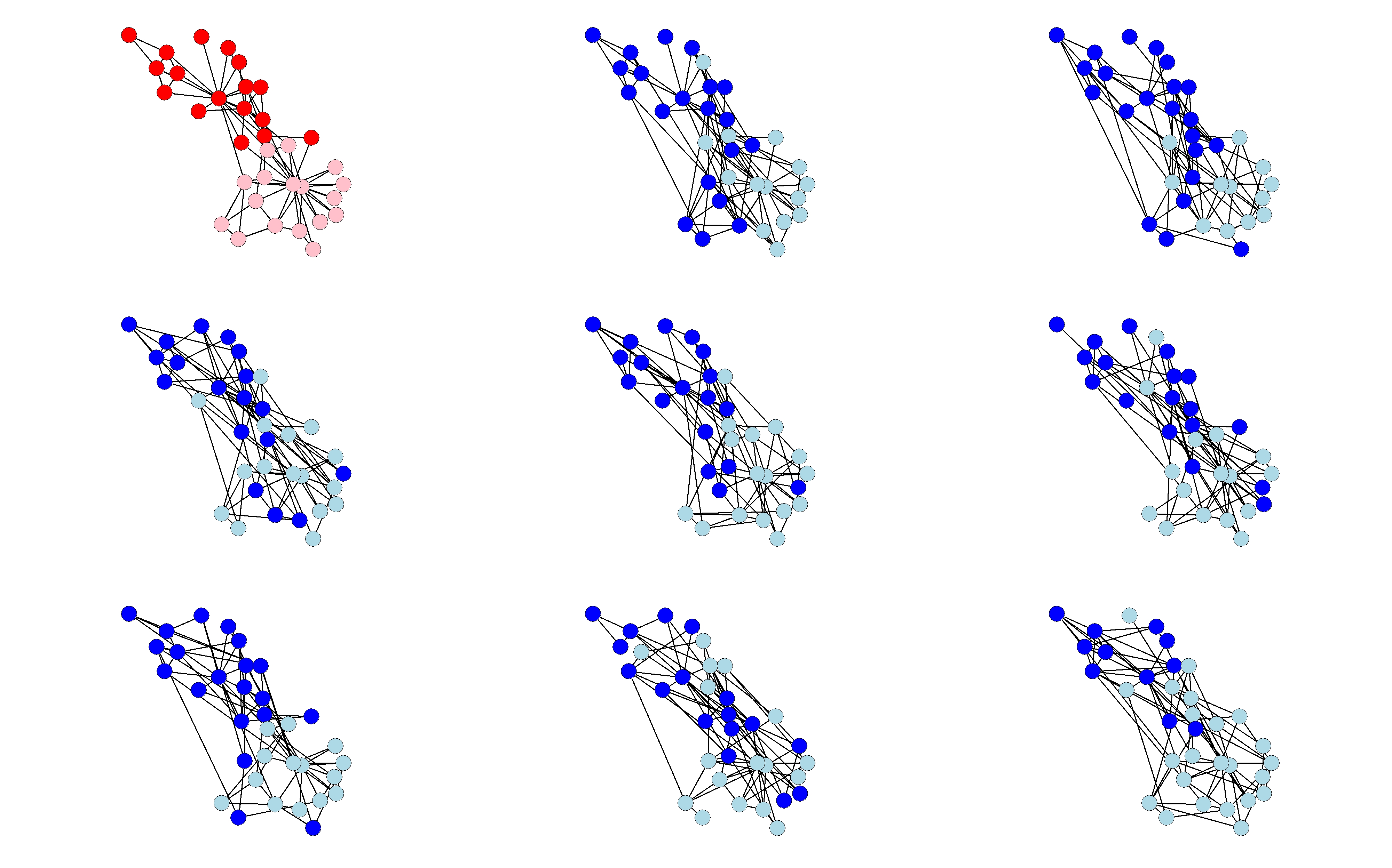
(a) Accepted batch

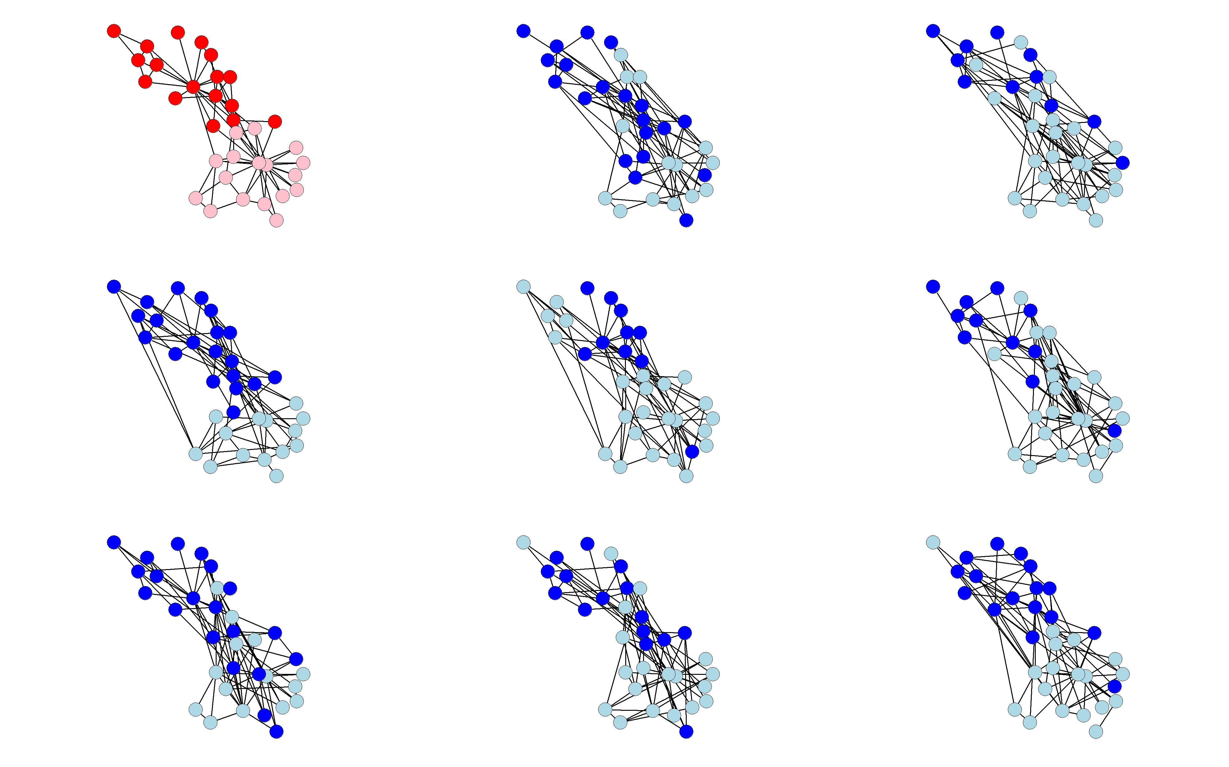
(b) Rejected batch

Figure 17: Rejected and accepted CELL-samples trained on Zarachy’s Karate Club network. The original graph is displayed in red, simulated graphs are displayed in blue. Different shadings indicate the cluster membership. The layout is kept fixed for all graphs. We observe no significant difference between the accepted and rejected sample in how well cluster membership in the simulated samples corresponds to cluster membership in the original graph.

Appendix C Runtime considerations

C.1 Runtime experiments

Here we present the runtimes for calculating sampled gKSS with sample size $B=200$ using the kernel implementations by the R package graphkernel. We use an Edge-2Star model with parameters $\beta=(-2,0)$ (sparse regime, average edge density 11.8%) and $\beta=(1,0)$ (dense regime, average edge density 73.2%) for $n=20$ and $n=40$ vertices. For a given graph, we run each kernel ten times on the graph and pick the median runtime to largely remove randomness in the runtime due to the momentary performance of the machine from the runtime analysis. For each of the four set-ups, we repeat this procedure for 100 different graphs, obtaining 100 median runtimes per set-up. We report their minimum, average and maximum for every kernel. We consider different hyperparameters for the kernels, to assess whether the hyperparameter affects the computational complexity of the algorithm.

	Runtime (ms) for $n=20$, sparse			Runtime (ms) for $n=40$, sparse
Kernel	Minimum	Average	Maximum	Minimum	Average	Maximum
Const.	0.47	0.50	1.03	0.51	0.57	1.10
WL 1	199.51	206.42	214.23	219.38	224.10	233.86
WL 3	201.54	210.59	218.99	229.06	235.09	242.58
WL 5	208.74	218.26	225.49	245.64	255.18	267.64
GLET 3	192.08	202.50	214.43	311.96	326.72	345.26
GVEH	318.32	331.63	342.52	428.01	448.00	470.37
CONGLET 3	385.88	400.35	417.83	512.63	539.49	560.63
CONGLET 4	379.00	407.84	438.10	620.05	754.20	968.26
KRW 3	432.39	682.93	1,010.08	3,638.44	5,460.50	7,713.08
KRW 5	432.76	682.45	1,008.46	3,616.95	5,463.80	7,715.39
GRW	427.29	678.56	1,002.74	3,590.22	5,473.98	7,725.11
SP	655.11	940.04	1,278.72	4,071.83	5,984.19	8,280.77

Table 6: Runtime of graph kernels with different hyperparameters on sparse graphs of size 20 and 40 in milliseconds. The sparse graphs are simulated from an E2S-model with parameters $\beta=(-2,0)$.

	Runtime (ms) for $n=20$, dense			Runtime (ms) for $n=40$, dense
Kernel	Minimum	Average	Maximum	Minimum	Average	Maximum
Const.	0.47	0.53	1.04	0.51	0.54	1.12
WL 1	210.82	217.08	224.71	245.06	253.82	415.35
WL 3	215.61	227.18	235.57	268.51	290.70	460.15
WL 5	235.62	243.09	249.93	319.81	351.17	376.40
GLET 3	212.13	219.29	230.56	406.23	447.68	482.55
GVEH	366.71	384.54	405.73	581.44	640.82	890.56
CONGLET 3	425.63	444.61	466.28	644.86	796.21	928.90
CONGLET 4	2,145.85	2,439.85	2,838.56	16,114.99	41,525.31	54,248.50
KRW 3	9,241.91	10,184.59	11,846.73	72,359.72	135,137.37	165,997.28
KRW 5	9,225.76	10,188.56	11,801.09	72,578.23	135,177.07	165,510.63
GRW	9,206.17	10,222.37	11,985.30	72,276.88	135,096.51	165,456.58
SP	9,767.99	10,706.33	12,311.66	74,118.71	136,571.69	166,649.77

Table 7: Runtime of graph kernels with different hyperparameters on dense graphs of size 20 and 40 in milliseconds. The dense graphs are simulated from an E2S-model with parameters $\beta=(1,0)$.

The results are shown in Table 6, for sparse networks, and Table 7, for dense networks. The constant kernel is the quickest to evaluate by two orders of magnitude compared to the runner-up. The fastest non-trivial choice is the Weisfeiler-Lehman kernel, with which gKSS on average takes about 0.2 to 0.35 seconds to calculate. The runtime is very consistent in every set-up with only little deviation and only slightly increases with increased level or density. Similarly, gKSS using the Gaussian vertex-edge histogram kernel takes between around 0.33 seconds to compute on the network of 20 vertices and 0.45 seconds on the network of 40 vertices, with no large increase in runtime on the denser networks.

For the graphlet kernel on three vertices, it takes roughly 0.2 seconds to calculate gKSS on the network on 20 vertices and 0.33 seconds on the network of 40 vertices. As the number of triplets of vertices which need to be checked for calculating the kernel is independent of the edge structure of the graph, there is little difference in runtime for the sparse or dense network. This is very different for the connected graphlet kernel as an action such as increasing the count of a certain graphlet is only needed if the vertex set that is currently examined by the algorithm is connected. Using the connected graphlet kernel takes longer than the graphlet kernel as additional checks for connectivity are needed. In the sparse regime, runtimes of the kernel on graphlets of size 3 or 4 are comparable, with a runtime of 0.4 seconds for both on 20 vertices and a runtime of 0.54 and 0.75 seconds on 40 vertices. However, a large disparity emerges in the dense regime: Whereas, for graphlets of size 3, the kernel takes 0.44 seconds on the smaller and 0.8 seconds on the bigger network, for graphlets of size 4, runtimes increase to 2.4 seconds on 20 vertices and even 41.5 seconds on 40 vertices.
Both the $k$-Random Walk kernels and the Geometric Random Walk kernel have a similar runtime, irrespective of the chosen hyperparameters. While their runtime is still competitive on the smaller and sparser graphs, their runtime increases by an order of magnitude when doubling the number of vertices or moving from the sparse to the dense regime. The slowest of the kernels is the shortest path kernel, though its runtime is largely comparable to the random walk kernels. In the sparse case it runs on average for 0.94 seconds on the smaller and 5.9 seconds on the larger network. In the dense case, however, runtime increases to 10.7 seconds for the smaller and to more than 2 minutes in the larger network. This renders the kernel in its current implementation unserviceable in practice. The reasons for this are twofold: Firstly, unlike the other kernels, its code is written in Python and not C++, thus making the implementation slower irrespective of the used algorithm. Secondly, the authors use a basic approach for calculation of the shortest path graph by running Dijkstra’s algorithm for every vertex. This means that even with optimal data storage implementation, the runtime complexity of the algorithm for a graph on $n$ vertices and $m$ edge is $O(n^{2}\log(n)+nm)$ steps Cormen et al., (2022). Generally, kernels considering paths in the graph have the longest runtimes and their comparative disadvantage becomes worse the larger and denser the network becomes. Furthermore, unlike the other kernels, their runtime varies greatly even in the same regime, so calculation times may strongly deviate from the average.

As kernel implementation may have a considerable effect on the runtime, next we detail a computationally efficient implementation of GRW kernels.

C.2 Efficient computation for GRW kernels

The GRW kernel with parameter $\lambda$ for networks $x,x^{\prime}$ is $k_{GRW}^{\lambda}(x,x^{\prime})=\sum_{i,j=1}^{|V_{\otimes}|}\left[(I-\lambda A_{\otimes})^{-1}\right]_{i,j}=\mathbf{1}_{n}^{T}(I_{n}-\lambda A_{\otimes})^{-1}\mathbf{1}_{n}.$ . This expression involves inverting a $n\times n$ matrix, at cost $O(n^{3})$. Due to the special form of KSS the following theorem shows that $O(n)$ computation cost suffices.

Theorem 1.

Let $B$ be a symmetric invertible matrix and $C=B^{-1}$. Let $C_{i}$ denote the $i$-th column and $c_{ij}$ the $(i,j)$-th entry of $C$; $e_{i}$ is the $i$-th coordinate vector. Let $\mu\in\mathbb{R}$ satisfy $1+\mu c_{ij}\neq 0$ and $(1+\mu c_{ij})^{2}-\mu^{2}c_{ii}c_{jj}\neq 0$. Then $M=(B+\mu(e_{i}e_{j}^{T}+e_{j}e_{i}^{T}))$ is invertible and

$$M^{-1}=C-\frac{\mu(1+\mu c_{ij})}{(1+\mu c_{ij})^{2}-\mu^{2}c_{ii}c_{jj}}(C_{i}C^{T}_{j}+C_{j}C^{T}_{i}-\frac{\mu c_{jj}}{1+\mu c_{ij}}C_{i}C^{T}_{i}-\frac{\mu c_{ii}}{1+\mu c_{ij}}C_{j}C^{T}_{j}).$$ (11)

For $A_{\otimes}=A-(e_{i}e_{j}^{T}+e_{j}e_{i}^{T})$ and $B=I_{n}-\lambda A$, taking $\mu=\lambda$ yields a fast rank 1 computation of $B_{\otimes}=I_{n}-\lambda A_{\otimes}$ for GRW kernels.

To prove 1, we apply the Sherman-Morrison formula (Sherman and Morrison,, 1950) (as a special case of Woodbury matrix identity); we repeat it here for convenience.

Proposition 1 (Sherman-Morrison).

Let $A\in\mathbb{R}^{n\times n}$ be an invertible matrix and let $u,v\in\mathbb{R}^{n}$ be column vectors. Then the matrix $A+uv^{T}$ is invertible if and only if $\mathbb{1}+v^{T}A^{-1}u\neq 0$, and in this case

$$(A+uv^{T})^{-1}=A^{-1}-\frac{1}{1+v^{T}A^{-1}u}A^{-1}uv^{T}A^{-1}.$$ (12)

Proof of 1

Proof.

The statement follows from applying 1 twice. First, we use the formula with $A=B$, $u=\mu e_{i}$, $v=e_{j}$ and note that as $1+\mu c_{ij}\neq 0$, we may apply the proposition. Then by the symmetry of the inverse matrix $C$

$$(B+\mu e_{i}e_{j}^{T})^{-1} =B^{-1}-\frac{1}{1+e_{j}^{T}B^{-1}\mu e_{i}}B^{-1}\mu e_{i}e_{j}^{T}B^{-1}$$

$$=C-\frac{\mu}{1+\mu c_{ij}}(Ce_{i})(e_{j}^{T}C)=C-\frac{\mu}{1+\mu c_{ij}}C_{i}C_{j}^{T}.$$ (13)

Applying the theorem again with $A=B+\mu e_{i}e_{j}^{T}$, $u=\mu e_{j}$, $v=e_{i}$ and assuming that $(1+\mu c_{ij})^{2}-\mu^{2}c_{ii}c_{jj}\neq 0$, we can calculate the inverse as

$$\big{(}(B+\mu e_{i}e_{j}^{T})+\mu e_{j}e_{i}^{T}\big{)}^{-1} = (B+\mu e_{i}e_{j}^{T})^{-1}-\frac{\mu}{1+e_{i}^{T}(B+\mu e_{i}e_{j}^{T})^{-1}\mu e_{j}}$$ (14)

$$\times\big{(}(B+\mu e_{i}e_{j}^{T})^{-1}e_{j}\big{)}\big{(}e_{i}^{T}(B+\mu e_{i}e_{j}^{T})^{-1}\big{)}.$$

We use the expression in Eq.(13) to calculate the terms of Eq.(14). We first calculate the $(ij)$-th entry

$$e_{i}^{T}(B+\mu e_{i}e_{j}^{T})^{-1}e_{j} =e_{i}^{T}Ce_{j}-\frac{\mu}{1+\mu c_{i,j}}(e_{i}^{T}C_{i})(C_{j}^{T}e_{j})=c_{ij}-\frac{\mu c_{ii}c_{jj}}{1+\mu c_{ij}}$$

$$=\frac{(1+\mu c_{ij})c_{ij}-\mu c_{ii}c_{jj}}{1+\mu c_{ij}},$$

with which the fraction in Eq.(14) calculates as

$$\frac{\mu}{1+e_{i}^{T}(B+\mu e_{i}e_{j}^{T})^{-1}\mu e_{j}}=\frac{\mu}{1+\mu(1+\mu c_{ij})^{-1}\{(1+\mu c_{ij})c_{ij}-\mu c_{ii}c_{jj}\}}$$

$$=\frac{\mu(1+\mu c_{ij})}{(1+\mu c_{ij})+\mu(1+\mu c_{ij})c_{ij}-\mu^{2}c_{i,i}c_{jj}}=\frac{\mu(1+\mu c_{ij})}{(1+\mu c_{ij})^{2}-\mu^{2}c_{ii}c_{jj}}.$$

Calculating the column vectors

$$(B+\mu e_{i}e_{j}^{T})^{-1}e_{j}=Ce_{j}-\frac{\mu}{1+\mu c_{ij}}C_{i}C_{j}^{T}e_{j}=C_{j}-\frac{\mu c_{jj}}{1+\mu c_{ij}}C_{i}$$

and

$$e_{i}^{T}(B+\mu e_{i}e_{j}^{T})^{-1}=C_{i}^{T}-\frac{\mu c_{ii}}{1+\mu c_{ij}}C_{j}^{T}.$$

Putting these expressions and Eq.(13) into Equation (14) yields the identity

$$(B+\mu(e_{i}e_{j}^{T}+e_{j}e_{i}^{T}))^{-1}=C-\frac{\mu}{1+\mu c_{ij}}C_{i}C_{j}^{T}-\frac{\mu(1+\mu c_{ij})}{(1+\mu c_{ij})^{2}-\mu^{2}c_{ii}c_{jj}}$$

$$\times\left(C_{j}C_{i}^{T}-\frac{\mu c_{jj}}{1+\mu c_{ij}}C_{i}C_{i}^{T}-\frac{\mu c_{ii}}{1+\mu c_{ij}}C_{j}C_{j}^{T}+\frac{\mu^{2}c_{ii}c_{jj}}{(1+\mu c_{ij})^{2}}C_{i}C^{T}_{j}\right).$$

The final form in Eq.(11) follows from the algebraic identity

$$\frac{\mu}{1+\mu c_{ij}}+\frac{\mu(1+\mu c_{ij})}{(1+\mu c_{ij})^{2}-\mu^{2}c_{ii}c_{jj}}\times\frac{\mu^{2}c_{ii}c_{jj}}{(1+\mu c_{ij})^{2}}=\frac{\mu(1+\mu c_{ij})}{(1+\mu c_{ij})^{2}-\mu^{2}c_{ii}c_{jj}}.$$

∎

The required criteria $1+\mu c_{ij}\neq 0$ and $(1+\mu c_{ij})^{2}-\mu^{2}c_{ii}c_{jj}\neq 0$ are sufficient but not necessary. See for example

$$B=\begin{bmatrix}1&1\\ 1&2\end{bmatrix},\ C=B^{-1}=\begin{bmatrix}2&-1\\ -1&1\end{bmatrix},\ \mu=1.$$

Then $1+\mu c_{12}=1-1=0$ and while neither $B+\mu e_{1}e_{2}^{T}$ nor $B+\mu e_{2}e_{1}^{T}$ are invertible, we have

$$B+\mu(e_{1}e_{2}^{T}+e_{2}e_{1}^{T})=\begin{bmatrix}1&2\\ 2&2\end{bmatrix},\ \big{(}B+\mu(e_{1}e_{2}^{T}+e_{2}e_{1}^{T})\big{)}^{-1}=\begin{bmatrix}-1&1\\ 1&-\frac{1}{2}\end{bmatrix}.$$

However, if criterion $1+\mu c_{ij}\neq 0$ is fulfilled, then the criterion $(1+\mu c_{ij})^{2}-\mu^{2}c_{ii}c_{jj}\neq 0$ is necessary and sufficient for $B+\mu(e_{i}e_{j}^{T}+e_{j}e_{i}^{T})$ to be invertible. This follows directly from the Sherman-Morrison in 1. Note further that if any of the two expressions $1+\mu c_{ij}$ and $(1+\mu c_{ij})^{2}-\mu^{2}c_{ii}c_{jj}$ are close to zero, then the formula may become numerically unstable.

References

- Ahmed et al., (2017) Ahmed, N. K., Neville, J., Rossi, R. A., Duffield, N. G., and Willke, T. L. (2017). Graphlet decomposition: Framework, algorithms, and applications. Knowledge and Information Systems, 50(3):689–722.
- Bhamidi et al., (2011) Bhamidi, S., Bresler, G., and Sly, A. (2011). Mixing time of exponential random graphs. The Annals of Applied Probability, 21(6):2146–2170.
- Borgwardt and Kriegel, (2005) Borgwardt, K. M. and Kriegel, H.-P. (2005). Shortest-path kernels on graphs. In Fifth IEEE International Conference on Data Mining (ICDM’05), pages 8–pp. IEEE.
- Chatterjee and Diaconis, (2013) Chatterjee, S. and Diaconis, P. (2013). Estimating and understanding exponential random graph models. The Annals of Statistics, 41(5):2428–2461.
- Chwialkowski et al., (2016) Chwialkowski, K., Strathmann, H., and Gretton, A. (2016). A kernel test of goodness of fit. In JMLR: Workshop and Conference Proceedings.
- Clauset et al., (2004) Clauset, A., Newman, M. E. J., and Moore, C. (2004). Finding community structure in very large networks. Physical Review E, 70(6).
- Cormen et al., (2022) Cormen, T. H., Leiserson, C. E., Rivest, R. L., and Stein, C. (2022). Introduction to Algorithms. MIT press.
- Frank and Strauss, (1986) Frank, O. and Strauss, D. (1986). Markov graphs. Journal of the American Statistical Association, 81(395):832–842.
- Gärtner et al., (2003) Gärtner, T., Flach, P., and Wrobel, S. (2003). On graph kernels: Hardness results and efficient alternatives. In Learning Theory and Kernel Machines, pages 129–143. Springer.
- Girvan and Newman, (2002) Girvan, M. and Newman, M. E. J. (2002). Community structure in social and biological networks. Proceedings of the National Academy of Sciences, 99(12):7821–7826.
- Gorham et al., (2020) Gorham, J., Raj, A., and Mackey, L. (2020). Stochastic stein discrepancies. In Advances in Neural Information Processing Systems, volume 33, pages 17931–17942.
- Holland and Leinhardt, (1981) Holland, P. W. and Leinhardt, S. (1981). An exponential family of probability distributions for directed graphs. Journal of the American Statistical Association, 76(373):33–50.
- (13) Hunter, D. R., Goodreau, S. M., and Handcock, M. S. (2008a). Goodness of fit of social network models. Journal of the American Statistical Association, 103(481):248–258.
- (14) Hunter, D. R., Handcock, M. S., Butts, C. T., Goodreau, S. M., and Morris, M. (2008b). ergm: A package to fit, simulate and diagnose exponential-family models for networks. Journal of Statistical Software, 24(3):nihpa54860.
- Kriege et al., (2016) Kriege, N. M., Giscard, P.-L., and Wilson, R. (2016). On valid optimal assignment kernels and applications to graph classification. In Advances in Neural Information Processing Systems, pages 1623–1631.
- Kriege et al., (2020) Kriege, N. M., Johansson, F. D., and Morris, C. (2020). A survey on graph kernels. Applied Network Science, 5(1):1–42.
- Ley et al., (2017) Ley, C., Reinert, G., and Swan, Y. (2017). Stein’s method for comparison of univariate distributions. Probability Surveys, 14:1–52.
- Liu et al., (2016) Liu, Q., Lee, J., and Jordan, M. (2016). A kernelized Stein discrepancy for goodness-of-fit tests. In International Conference on Machine Learning, pages 276–284.
- Penrose, (2003) Penrose, M. (2003). Random geometric graphs. Oxford University Press.
- Reinert and Ross, (2019) Reinert, G. and Ross, N. (2019). Approximating stationary distributions of fast mixing Glauber dynamics, with applications to exponential random graphs. The Annals of Applied Probability, 29(5):3201–3229.
- Rendsburg et al., (2020) Rendsburg, L., Heidrich, H., and Von Luxburg, U. (2020). NetGAN without GAN: From random walks to low-rank approximations. In International Conference on Machine Learning, pages 8073–8082. PMLR.
- Schrab et al., (2022) Schrab, A., Guedj, B., and Gretton, A. (2022). KSD aggregated goodness-of-fit test. arXiv preprint arXiv:2202.00824.
- Sherman and Morrison, (1950) Sherman, J. and Morrison, W. J. (1950). Adjustment of an inverse matrix corresponding to a change in one element of a given matrix. The Annals of Mathematical Statistics, 21(1):124–127.
- Shervashidze et al., (2011) Shervashidze, N., Schweitzer, P., Leeuwen, E. J. v., Mehlhorn, K., and Borgwardt, K. M. (2011). Weisfeiler-Lehman graph kernels. Journal of Machine Learning Research, 12(Sep):2539–2561.
- Shervashidze et al., (2009) Shervashidze, N., Vishwanathan, S., Petri, T., Mehlhorn, K., and Borgwardt, K. (2009). Efficient graphlet kernels for large graph comparison. In Artificial Intelligence and Statistics, pages 488–495. PMLR.
- Sugiyama and Borgwardt, (2015) Sugiyama, M. and Borgwardt, K. (2015). Halting in random walk kernels. In Advances in Neural Information Processing Systems, pages 1639–1647.
- Sugiyama et al., (2018) Sugiyama, M., Ghisu, M. E., Llinares-López, F., and Borgwardt, K. (2018). graphkernels: R and Python packages for graph comparison. Bioinformatics, 34(3):530–532.
- Wasserman and Faust, (1994) Wasserman, S. and Faust, K. (1994). Social Network Analysis: Methods and Applications. Cambridge University Press.
- Xu and Reinert, (2021) Xu, W. and Reinert, G. (2021). A Stein goodness-of-test for exponential random graph models. In International Conference on Artificial Intelligence and Statistics, pages 415–423. PMLR.
- Xu and Reinert, (2022) Xu, W. and Reinert, G. (2022). AgraSSt: Approximate graph stein statistics for interpretable assessment of implicit graph generators. arXiv preprint arXiv:2203.03673.
- Zachary, (1977) Zachary, W. W. (1977). An information flow model for conflict and fission in small groups. Journal of Anthropological Research, 33(4):452–473.