Low energy scattering asymptotics for planar obstacles

Abstract.

We compute low energy asymptotics for the resolvent of a planar obstacle, and deduce asymptotics for the corresponding scattering matrix, scattering phase, and exterior Dirichlet-to-Neumann operator. We use an identity of Vodev to relate the obstacle resolvent to the free resolvent and an identity of Petkov and Zworski to relate the scattering matrix to the resolvent. The leading singularities are given in terms of the obstacle’s logarithmic capacity or Robin constant. We expect these results to hold for more general compactly supported perturbations of the Laplacian on $\mathbb{R}^{2}$, with the definition of the Robin constant suitably modified, under a generic assumption that the spectrum is regular at zero.

1. Introduction

1.1. Main results

Consider the Dirichlet Laplacian $-\Delta$ on a planar exterior domain $\Omega=\mathbb{R}^{2}\setminus\mathscr{O}$, where $\mathscr{O}\subset\mathbb{R}^{2}$ is a compact set. We study three fundamental objects in the scattering theory of $-\Delta$ on $\Omega$: the resolvent, the scattering matrix, and the scattering phase. Each is a function of the frequency $\lambda$. Our main results are uniformly convergent series expansions for all three objects near $\lambda=0$. We also deduce asymptotics for the Dirichlet-to-Neumann operator and for its lowest eigenvalue.

We begin with the resolvent $R(\lambda)$, defined for $\operatorname{Im}\lambda>0$ to be the operator which takes $f\in L^{2}(\Omega)$ to the unique $u\in\mathcal{D}:=\{u\in H^{1}_{0}(\Omega)\colon\Delta u\in L^{2}(\Omega)\}$ solving $(-\Delta-\lambda^{2})u=f$. For every $\chi\in C_{0}^{\infty}(\mathbb{R}^{2}),$ the product $\chi R(\lambda)\chi$ extends meromorphically as an operator-valued function of $\lambda$ to $\Lambda$, the Riemann surface of the logarithm: see Section 1.4 for more on the notation used here and below.

For our main results we assume that $\mathscr{O}$ is not polar, i.e. that $C_{0}^{\infty}(\Omega)$ is not dense in $H^{1}(\mathbb{R}^{2}).$ For example, by Lemma A.1, it is enough if $\mathscr{O}$ contains a line segment.

Theorem 1.

Suppose $\mathscr{O}$ is not polar. Then there are operators $B_{2j,k}\colon L^{2}_{c}(\Omega)\to\mathcal{D}_{\text{loc}}$ (i.e. mapping compactly supported functions in $L^{2}(\Omega)$ to functions which are locally in $\mathcal{D}$) and a constant $a$, such that, for every $\chi\in C_{0}^{\infty}(\mathbb{R}^{2})$, we have

$$\begin{split}\chi R(\lambda)\chi&=\sum_{j=0}^{\infty}\sum_{k=-j-1}^{j}\chi B_{2j,k}\chi\lambda^{2j}(\log\lambda-a)^{k}\\ &=\chi B_{0,0}\chi+\chi B_{0,-1}\chi(\log\lambda-a)^{-1}+\chi B_{2,1}\chi\lambda^{2}(\log\lambda-a)+\cdots,\end{split}$$ (1.1)

with the series converging absolutely in the space of bounded operators $L^{2}(\Omega)\to\mathcal{D}$, uniformly on sectors near zero.

Remarks. 1. Our proof also shows that if $k\neq 0$, then $B_{2j,k}$ has finite rank. Moreover, there is a unique harmonic function $G$ in $\mathcal{D}_{\text{loc}}$ such that $\log|x|-G(x)$ is bounded as $|x|\to\infty$, and

$$B_{0,-1}=\frac{1}{2\pi}G\otimes G,\quad a=\log 2-\gamma-C(\mathscr{O})+\frac{\pi i}{2},\quad C(\mathscr{O}):=\lim_{|x|\to\infty}\log|x|-G(x).$$ (1.2)

The quantity $C(\mathscr{O})$ is important in potential theory. It is the negative of Robin’s constant and as the logarithm of the logarithmic capacity: see Appendix A.

2. We used the following definition, which will recur below: Given functions $f_{n}$ mapping $\Lambda$ to a Banach space $\mathcal{B}$, we say $\sum_{n}f_{n}(\lambda)$ converges absolutely in $\mathcal{B}$, uniformly on sectors near zero if, for any $\varphi>0$, there is $\lambda_{1}>0$ such that $\sum_{n}\|f_{n}(\lambda)\|_{\mathcal{B}}$ converges uniformly on $\{\lambda\in\Lambda\colon 0<|\lambda|\leq\lambda_{1}\text{ and }|\arg\lambda|\leq\varphi\}$. Moreover, the series (1.1), as well as the series (1.6) below, may be freely differentiated term by term, with each resulting series having a tail which converges absolutely in $\mathcal{B}$, uniformly on sectors near zero: see Appendix B.

3. If we used $\lambda^{2j}(\log\lambda)^{k}$ instead of $\lambda^{2j}(\log\lambda-a)^{k}$ in our expansion, in place of (1.1) we would get

$$\chi R(\lambda)\chi=\sum_{j=0}^{\infty}\sum_{k=-\infty}^{j}\chi\widetilde{B}_{2j,k}\chi\lambda^{2j}(\log\lambda)^{k}.$$ (1.3)

Note that terms in (1.3) with $j\geq 1$ have infinitely many predecessors, and hence (1.3) is an asymptotic expansion only as far as the terms with $j=0$. The technique of using a shift of the logarithm to reduce the number of terms comes from [Jen84].

Our second theorem concerns the scattering matrix $S(\lambda)$, which is a meromorphic family of operators $L^{2}(\mathbb{S}^{1})\to L^{2}(\mathbb{S}^{1})$. It can be defined for $\lambda\in\Lambda$ by Petkov and Zworski’s formula

$$S(\lambda)=I+A(\lambda),\qquad\text{where}\qquad A(\lambda)=\frac{1}{4\pi i}E(\lambda)[\Delta,\chi_{1}]R(\lambda)[\Delta,\chi_{2}]E(\overline{\lambda})^{*}.$$ (1.4)

Here $E(\lambda)$ is the operator from $L^{2}(\mathbb{R}^{2})$ to $L^{2}(\mathbb{S}^{1})$ which has integral kernel $e^{-i\lambda\omega\cdot x}\chi_{3}(x)$, and $\chi_{1},\ \chi_{2},\ \chi_{3}$ are radial functions in $C_{0}^{\infty}(\mathbb{R}^{2})$ obeying

$$\chi_{1}\equiv 1\text{ near }\overline{D_{\rho}},\qquad\chi_{i}\equiv 1\text{ near supp }\chi_{i-1},\qquad 0\leq\chi_{i}\leq 1,$$ (1.5)

where $\rho$ is large enough that $\mathscr{O}\subset D_{\rho}$, and $D_{\rho}=\{x\in\mathbb{R}^{2}\colon|x|<\rho\}$. The formula (1.4) comes from Theorem 4.26 of [DyZw19], and is a variant of the original Proposition 2.1 of [PeZw01].

Theorem 2.

Suppose $\mathscr{O}$ is not polar. Then there are finite rank operators $S_{j,k}\colon L^{2}(\mathbb{S}^{1})\to L^{2}(\mathbb{S}^{1})$, such that

$$\begin{split}S(\lambda)&=I+\frac{i}{2}(1\otimes 1)(\log\lambda-a)^{-1}+S_{1,-1}\lambda(\log\lambda-a)^{-1}+\sum_{j=2}^{\infty}\sum_{k=-\lfloor j/2\rfloor-1}^{\lfloor j/2\rfloor}S_{j,k}\lambda^{j}(\log\lambda-a)^{k},\end{split}$$ (1.6)

with the series converging absolutely in the space of trace-class operators $L^{2}(\mathbb{S}^{1})\to L^{2}(\mathbb{S}^{1})$, uniformly on sectors near zero.

Our third theorem concerns the scattering phase $\sigma(\lambda)$ for $\lambda$ near zero, defined by

$$\sigma(\lambda)=\frac{1}{2\pi i}\log\det S(\lambda)=\frac{1}{2\pi i}\operatorname{tr}\log S(\lambda).$$ (1.7)

Theorem 3.

Suppose $\mathscr{O}$ is not polar. Then there are complex numbers $a_{2j,k}$ and $b_{2j,k}$ such that

$$\sigma(\lambda)=\frac{1}{2\pi i}\log\Big{(}1+\frac{i\pi}{\log\lambda-a}\Big{)}+\sum_{j=1}^{\infty}\sum_{k=-\infty}^{j}a_{2j,k}\lambda^{2j}(\log\lambda-a)^{k},$$ (1.8)

and

$$\sigma^{\prime}(\lambda)=\frac{-1}{2\lambda(\log\lambda-a)(\log\lambda-\bar{a})}+\sum_{j=1}^{\infty}\sum_{k=-\infty}^{j}b_{2j-1,k}\lambda^{2j-1}(\log\lambda-a)^{k},$$ (1.9)

with the series converging absolutely in $\mathbb{C}$, uniformly on sectors near zero. In particular, as $\lambda\to 0$ through positive real values, we have

$$\sigma(\lambda)=\frac{1}{\pi}\arctan\Big{(}\frac{\pi}{2\log(\lambda/2)+2C(\mathscr{O})+2\gamma}\Big{)}+O(\lambda^{2}\log\lambda),$$ (1.10)

and

$$\sigma^{\prime}(\lambda)=\frac{-2/\lambda}{4(\log(\lambda/2)+C(\mathscr{O})+\gamma)^{2}+\pi^{2}}+O(\lambda\log\lambda).$$ (1.11)

Remark. In each of the theorems above, the assumption that $\mathscr{O}$ is not polar is necessary as well as sufficient. Indeed, if $\mathscr{O}$ is polar, then the expansion near $\lambda=0$ of $R(\lambda)$ is not of the form (1.1) but instead equals that of the free resolvent (2.4). Moreover, $S(\lambda)=I$ and $\sigma(\lambda)=0$ for all $\lambda$. To see this, note that if $\mathscr{O}$ is polar, then $H^{1}_{0}(\Omega)$, the form domain of the Dirichlet Laplacian on $\Omega$, is dense in $H^{1}(\mathbb{R}^{2})$, the form domain of the free Laplacian on $\mathbb{R}^{2}$. Consequently the continuous extension of $R(\lambda)$ from $L^{2}(\Omega)$ to $L^{2}(\mathbb{R}^{2})$ equals the free resolvent $R_{0}(\lambda)$ of Section 2.1.

1.2. Background and context

Early low frequency resolvent expansions were obtained by MacCamy [Mac65]. Vainberg [Vai75, Vai89] has very general results and many references. We focus on dimension two because of its physical importance and because the problem is harder here than in other dimensions; see for example Lemma 2.3 in [LaPh72] by Lax and Phillips for an expansion of the scattering matrix in dimension three.

Our Theorem 1 is a variant of Theorem 2 of [WeWi92] by Weck and Witsch, of Theorem 1 of [KlVa94] by Kleinman and Vainberg, and of Theorem 1.7 of [StWa20] by Strohmaier and Waters.

More specifically, the results of [KlVa94] and [StWa20] cover problems which are more general than ours in many respects, but specialized to our setting they require $\partial\Omega$ to be $C^{\infty}$, while our assumption that $\mathscr{O}$ is polar is optimal. The results of [WeWi92] expand only up to $O(\lambda^{2})$. Our methods are different from those in the papers mentioned above. Specifically, [KlVa94] and [StWa20] rely on general theory developed in [Vai89] and [MüSt14] respectively, while our approach based on algebra of series of operators as in Vodev [Vod99, Vod14] leads to a direct short proof of complete resolvent asymptotics: see Section 2.

Our scattering phase asymptotic (1.10) improves previous results in [HaZe99] and [McG13], and is implicit in the proof of Theorem 3.25 of [StWa20]. To compare the results, recall that in [McG13], McGillivray computes asymptotics of the Krein spectral shift function $\xi$ defined by

$$\operatorname{tr}\Big{(}Jg(H)J^{*}-g(-\Delta)\Big{)}=\int_{0}^{\infty}g^{\prime}(\mu)\xi(\mu)d\mu,$$

where $J$ is the operator taking functions on $\mathbb{R}^{2}\setminus\overline{\mathscr{O}}$ to functions on $\mathbb{R}^{2}$ by extending them by zero. By the Birman–Krein formula (see [JeKa78] or Proposition 0.1 and Theorem 1.1 of [Chr98]), we see that $\xi(\mu)=-\sigma(\sqrt{\mu})$. Putting $b=\log 4-2C(\mathscr{O})-2\gamma$ and applying (1.10) gives

$$\xi(\mu) =\frac{1}{\pi}\arctan\Big{(}\frac{\pi}{b-\log\mu}\Big{)}+O(\mu\log\mu)$$ (1.12)

$$=\frac{1}{-\log\mu}+\frac{-b}{(-\log\mu)^{2}}+\frac{b^{2}-\frac{\pi^{2}}{3}}{(-\log\mu)^{3}}+O((\log\mu)^{-4}).$$ (1.13)

Thus, (1.12) recovers and improves (1.13). The first term of (1.13) was first computed in [HaZe99], and all three terms of (1.13) were computed in [McG13] (note that $C(K)$ in [McG13] corresponds to $2C(\mathscr{O})$ here). See Figure 1 for a comparison of the approximations when the obstacle $\mathscr{O}$ is a disk of radius $\rho$, in which case the spectral shift function is given by

$$\xi_{\rho}(\mu)=\frac{1}{2\pi}\sum_{\ell=-\infty}^{\infty}\arg\big{(}H^{(2)}_{\ell}(\rho\sqrt{\mu})/H^{(1)}_{\ell}(\rho\sqrt{\mu})\big{)};$$ (1.14)

see (C.1). Note that the scaling $\xi_{\rho}(\mu)=\xi_{1}(\rho^{2}\mu)$ exhibited by (1.14) is also respected by our approximation in (1.12), but not by the individual terms of (1.13).

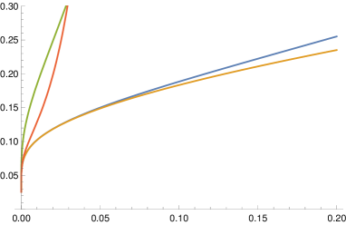
Figure 1. Graphs of the spectral shift function $\xi$ and its first three approximations, when the obstacle $\mathscr{O}$ is a disk of radius $\rho=$ 0.15 (top left), 1.5 (top right), 15 (bottom left), and 150 (bottom right). The horizontal axis is the dimensionless (scaling-invariant) variable $\rho\lambda=\rho\sqrt{\mu}$. The blue is the true value (1.14). The green is the first term from (1.13), first obtained in [HaZe99]. The red is the first three terms from (1.13), first obtained in [McG13]. The yellow is the leading approximation obtained in this paper, given by the first term of (1.12), which is implicit in the proof of Theorem 3.25 of [StWa20]. Observe that the yellow and blue curves are independent of the radius $\rho$, while the red and green depend on $\rho$.

More recently, in [GMWZ22], more accurate analytic and numerical investigations of the scattering phase have been conducted for both a disk and for other obstacles, including ones with different kinds of stable and unstable trapping.

1.3. Discussion of methods and outline of proof

The method of proof is as follows. In Section 2, we deduce the series for the resolvent $R(\lambda)$ of Theorem 1 from the series for the free resolvent $R_{0}(\lambda)$, using a resolvent identity due to Vodev [Vod14], and techniques in part based on Vodev’s work in [Vod99].

Our techniques can be applied to quite general compactly supported perturbations of $-\Delta$ on $\mathbb{R}^{2}$, far beyond the specific, classical setting considered here, that of the Dirichlet problem on an exterior domain. In a companion paper we will address the more general case. As demonstrated already in [BGD88, JeNe01] for the case of Schrödinger operators on $\mathbb{R}^{2}$, different kinds of singular behavior of the resolvent near zero can then appear.

We deduce the series for the scattering matrix and scattering phase of Theorems 2 and 3 in Section 3, by inserting the resolvent expansion (1.1) into the formulas (1.4) and (1.7). Section 4 contains some related results for the Dirichlet-to-Neumann operator.

Appendix A collects background on polar and nonpolar sets, Appendix B contains a lemma about series with logarithmic terms, and Appendix C contains formulas for the scattering matrix and scattering phase of a disk; see also Section 5.2 of [HaZe99] and Section 3 of [GMWZ22].

The presentation of Theorems 1, 2, and 3 is self-contained, based on standard complex and functional analysis, except for a few ingredients. For the resolvent expansions we quote the series (2.1) and (2.2) for the free resolvent. For the scattering matrix and scattering phase we quote Petkov and Zworski’s formula (1.4). Our analysis of the Dirichlet-to-Neumann operator in Section 4 requires more, namely mapping properties from [GMZ07], results on solutions of boundary value problems from [McL00], and results on analyticity of eigenvalues for which [ReSi78] is a reference.

1.4. Notation and conventions

• $C_{0}^{\infty}(U)$ is the set of functions in $C^{\infty}(U)$ with compact support in $U$.

• $\mathscr{O}\subset\mathbb{R}^{2}$ is compact and $\Omega=\mathbb{R}^{2}\setminus\mathscr{O}$. We say $\mathscr{O}$ is polar if $C_{0}^{\infty}(\Omega)$ is dense in $H^{1}(\mathbb{R}^{2})$. The Dirichlet Laplacian is $-\Delta\colon\mathcal{D}\to L^{2}(\Omega)$, with $\mathcal{D}=\{u\in H^{1}_{0}(\Omega)\colon\Delta u\in L^{2}(\Omega)\}$, and $\Delta:=\partial_{x_{1}}^{2}+\partial_{x_{2}}^{2}$.

• The Dirichlet resolvent $R(\lambda)$ is defined for $\operatorname{Im}\lambda>0$ to be the operator which takes $f\in L^{2}(\Omega)$ to the unique $u\in\mathcal{D}$ solving $(-\Delta-\lambda^{2})u=f$. For every $\chi\in C_{0}^{\infty}(\mathbb{R}^{2})$, the product $\chi R(\lambda)\chi$ continues meromorphically from the upper half plane to $\Lambda$, the Riemann surface of the logarithm. The free resolvent $R_{0}(\lambda)$ is defined in the same way but with $L^{2}(\Omega)$ replaced by $L^{2}(\mathbb{R}^{2})$ and $\mathcal{D}$ replaced by $H^{2}(\mathbb{R}^{2})$. See Sections 2.1 and 2.3 for a review of these facts.

• The mapping $\Lambda\to\mathbb{C}$ given by $\lambda\mapsto\log\lambda$ is bijective, with the upper half plane $\operatorname{Im}\lambda>0$ identified with the subset of $\Lambda$ where $\arg\lambda=\operatorname{Im}\log\lambda$ takes values in $(0,\pi)$.

• The mapping $\lambda\mapsto\bar{\lambda}$ on $\Lambda$ is defined by $|\bar{\lambda}|=|\lambda|$ and $\arg\bar{\lambda}=-\arg\lambda$.

• The product of a function $\chi$ on $\mathbb{R}^{2}$ and a function $f$ on $\Omega$ is the function $\chi f$ on $\Omega$ obtained by ignoring the values of $\chi$ on $\mathbb{R}^{2}\setminus\Omega$.

• $L^{2}_{c}(\Omega)$ is the set of functions $f\in L^{2}(\Omega)$ such that $\chi f=f$ for some $\chi\in C_{0}^{\infty}(\mathbb{R}^{2})$. Other function spaces with a ‘c’ subscript are defined analogously.

• $\mathcal{D}_{\text{loc}}$ is the set of functions $f$ on $\Omega$ such that $\chi f\in\mathcal{D}$ for all $\chi\in C_{0}^{\infty}(\mathbb{R}^{2})$. Other function spaces with a ‘loc’ subscript are defined analogously.

• $G$ is the unique harmonic function in $\mathcal{D}_{\text{loc}}$ such that $\log|x|-G(x)$ is bounded as $|x|\to\infty$. We construct $G$ and prove its uniqueness in Lemma 2.6.

• $C(\mathscr{O})=\lim_{|x|\to\infty}\log|x|-G(x)$.

• $\gamma$ is Euler’s constant, given by $\gamma=-\Gamma^{\prime}(1)=0.577\dots$.

• $a=\log 2-\gamma-C(\mathscr{O})+\frac{\pi i}{2}$.

• $g\otimes h$ means the operator of rank one which maps $f$ to $(\int\overline{h}f)g$.

• Petkov and Zworski’s formula for the scattering matrix $S(\lambda)=I+A(\lambda)$ is given in (1.4). This corresponds to the definition $S(\lambda)=S_{a}(\lambda)S_{a,0}(\lambda)^{-1}$, where $S_{a}$ is the absolute scattering matrix and $S_{a,0}$ is the free absolute scattering matrix, as in Section 4.4.3 of [DyZw19]. Note that the convention in [PeZw01], as in [Mel95], has instead $S(\lambda)=S_{a,0}(\lambda)^{-1}S_{a}(\lambda)$.

• The cutoff functions $\chi_{1}$, $\chi_{2}$, and $\chi_{3}$ are introduced in (1.5).

• The scattering phase is $\sigma(\lambda)=\frac{1}{2\pi i}\log\det S(\lambda)=\frac{1}{2\pi i}\operatorname{tr}\log S(\lambda)$. This definition gives the same value for either convention of $S(\lambda)$.

• $\mathbb{N}=\{1,\,2\,\dots\}$ and $\mathbb{N}_{0}=\{0\}\cup\mathbb{N}$.

2. The resolvent

2.1. The free resolvent

Let $R_{0}(\lambda)$ be the free resolvent on $\mathbb{R}^{2}$, defined for $\operatorname{Im}\lambda>0$ to be the operator which takes $f\in L^{2}(\mathbb{R}^{2})$ to the unique $u\in H^{2}(\mathbb{R}^{2})$ solving $(-\Delta-\lambda^{2})u=f$. The integral kernel of $R_{0}(\lambda)$ is given in terms of Bessel functions of order $0$ by

$$R_{0}(\lambda)(x,y)=\frac{1}{2\pi}K_{0}(-i\lambda|x-y|)=\frac{i}{4}H^{(1)}_{0}(\lambda|x-y|),$$ (2.1)

where

$$H^{(1)}_{0}(\lambda)=\left(1+\frac{2i}{\pi}\log\left(\frac{\lambda}{2}\right)\right)J_{0}(\lambda)-\frac{2i}{\pi}\sum_{m=0}^{\infty}\psi(m+1)\frac{(-\lambda^{2}/4)^{m}}{(m!)^{2}},\qquad J_{0}(\lambda)=\sum_{m=0}^{\infty}\frac{(-\lambda^{2}/4)^{m}}{(m!)^{2}},$$

and $\psi$ is the digamma function, i.e. $\psi(1)=\Gamma^{\prime}(1)=-\gamma$, $\psi(m+1)=\psi(m)+\frac{1}{m}$; see e.g. [Bor20, Section 4.1.3] and [Olv97, Sections 2.9.3, 7.5, and 7.8.1]. Thus,

$$H^{(1)}_{0}(\lambda)=\sum_{m=0}^{\infty}\left(\frac{2i}{\pi}\log\left(\frac{\lambda}{2}\right)-\frac{2i}{\pi}\psi(m+1)+1\right)\frac{(-\lambda^{2}/4)^{m}}{(m!)^{2}}.$$ (2.2)

By large argument Bessel function asymptotics, (see e.g. [Olv97, Section 7.4.1]), for any $\lambda$ in the upper half plane we have $|R_{0}(\lambda)(x,y)|=O(e^{-|x-y|\operatorname{Im}\lambda})$. Hence, for any $f\in L^{2}_{c}(\mathbb{R}^{2})$ and $\lambda$ in the upper half plane,

$$R_{0}(\lambda)f(x)=O(e^{-|x|\operatorname{Im}\lambda}),\qquad\text{as }|x|\to\infty.$$ (2.3)

It follows from (2.1) and (2.2) that $R_{0}(\lambda)(x,y)$, and hence also $R_{0}(\lambda)\colon L^{2}_{c}(\mathbb{R}^{2})\to H^{2}_{\text{loc}}(\mathbb{R}^{2})$, continue holomorphically from the upper half plane to $\Lambda$, the Riemann surface of $\log\lambda$. For each $\lambda\in\Lambda$ we write

$$R_{0}(\lambda)=\sum_{j=0}^{\infty}\sum_{k=0}^{1}R_{2j,k}\lambda^{2j}(\log\lambda)^{k}=R_{01}\log\lambda+\tilde{R}_{0}(\lambda),$$ (2.4)

where $\tilde{R}_{0}(\lambda)$ is defined by the equation, the $R_{2j,k}$ are operators $L^{2}_{c}(\mathbb{R}^{2})\to H^{2}_{\text{loc}}(\mathbb{R}^{2})$ such that $\chi R_{2j,k}\chi$ is bounded $L^{2}(\mathbb{R}^{2})\to H^{2}(\mathbb{R}^{2})$ for any $\chi\in C_{0}^{\infty}(\mathbb{R}^{2})$, and the series converges in the sense that, for every $\lambda_{0}>0$ and $\chi\in C_{0}^{\infty}(\mathbb{R}^{2})$, the series

$$\sum_{j=1}^{\infty}\sum_{k=0}^{1}\|\chi R_{2j,k}\chi\|_{L^{2}(\mathbb{R}^{2})\to H^{2}(\mathbb{R}^{2})}|\lambda|^{2j}|\log\lambda|^{k}$$

converges uniformly for all $\lambda\in\Lambda$ with $|\lambda|\leq\lambda_{0}$.

The leading coefficient is

$$R_{01}=-\frac{1}{2\pi}(1\otimes 1),$$

where $1\otimes 1$ means the operator mapping $\varphi$ to the constant $\int_{\mathbb{R}^{2}}\varphi$. The next term has integral kernel

$$R_{00}(x,y)=-\frac{1}{2\pi}\log|x-y|+\frac{\log 2-\gamma}{2\pi}+\frac{i}{4}.$$

Since $\log|x-y|=\frac{1}{2}\log|x-y|^{2}=\log|x|+\frac{1}{2}\log(1-\frac{2x\cdot y}{|x|^{2}}+\frac{|y|^{2}}{|x|^{2}})$, we obtain

$$R_{00}f\,(x)=\Big{(}-\frac{1}{2\pi}\log|x|+\frac{\log 2-\gamma}{2\pi}+\frac{i}{4}\Big{)}\int_{\mathbb{R}^{2}}f+\frac{1}{4\pi}\sum_{m=1}^{\infty}\frac{1}{m|x|^{2m}}\int(2x\cdot y-|y|^{2})^{m}f(y)\,dy,$$ (2.5)

for $|x|$ large enough, when $f\in L^{2}_{c}(\mathbb{R}^{2})$.

2.2. The Dirichlet resolvent

Recall that the Dirichlet Laplacian $-\Delta$ is the unique operator $\mathcal{D}:=\{u\in H^{1}_{0}(\Omega)\colon\Delta u\in L^{2}(\Omega)\}\to L^{2}(\Omega)$ such that

$$\int_{\Omega}\nabla u\cdot\nabla v=\int_{\Omega}(-\Delta u)v,\qquad\text{for all }u\in\mathcal{D}\text{ and }v\in H^{1}_{0}(\Omega);$$ (2.6)

see the first two pages of Section 2 of Chapter 8 of [Tay11], or Section 6.1.2 of [Bor20].

From the fact that $-\Delta\colon\mathcal{D}\to L^{2}(\Omega)$ is nonnegative, we know that $\|R(i\kappa)\|_{L^{2}(\Omega)\to L^{2}(\Omega)}=\kappa^{-2}$ for all $\kappa>0$. We begin our analysis of the resolvent near $\kappa=0$ by showing that

$$\sup_{\kappa\in(0,1]}\|\kappa^{3/2}R(i\kappa)\chi\|_{L^{2}(\Omega)\to H^{1}_{0}(\Omega)}<\infty,\qquad\text{for all }\chi\in C_{0}^{\infty}(\mathbb{R}^{2}).$$ (2.7)

The bound (2.7) follows from $\|\chi f\|_{L^{4/3}}\leq\|\chi\|_{L^{4}}\|f\|_{L^{2}}$ (by Hölder’s inequality, Theorem 189 of [HLP34]) and the following lemma based on a Sobolev interpolation inequality of Ladyzhenskaya.

Lemma 2.1.

Let $\kappa>0$, $g\in L^{2}(\Omega)\cap L^{4/3}(\Omega)$, and $u=R(i\kappa)g$. Then

$$\|\nabla u\|_{L^{2}(\Omega)}^{2}+\kappa^{2}\|u\|_{L^{2}(\Omega)}^{2}\leq\frac{1}{\kappa\sqrt{8}}\|g\|_{L^{4/3}(\Omega)}^{2}.$$ (2.8)

Proof.

By (2.6) with $u=v$, and using Hölder’s inequality, we have

$$\int_{\Omega}|\partial_{x_{1}}u|^{2}+\int_{\Omega}|\partial_{x_{2}}u|^{2}+\kappa^{2}\int_{\Omega}|u|^{2}=\int_{\Omega}g\,\bar{u}\leq\|g\|_{L^{4/3}}\|u\|_{L^{4}}.$$

By equation (7.2) of Chapter 4 of [Tay11], if $u\in H^{1}_{0}(\Omega)$ then $u\in H^{1}_{0}(\mathbb{R}^{2})$, where we identify $u$ with its extension by $0$ from $\Omega$ to $\mathbb{R}^{2}$. As in Supplement 2 of Chapter 1 of [Lad85], we use $|\varphi(t)|=\frac{1}{2}|\int_{-\infty}^{t}\varphi^{\prime}-\int_{t}^{\infty}\varphi^{\prime}|\leq\frac{1}{2}\int_{\mathbb{R}}|\varphi^{\prime}|$ to obtain

$$\begin{split}\int_{\mathbb{R}^{2}}|u|^{4}&\leq\int_{\mathbb{R}}\ \sup_{x_{1}\in\mathbb{R}}|u(x_{1},x_{2})|^{2}\,dx_{2}\int_{\mathbb{R}}\ \sup_{x_{2}\in\mathbb{R}}|u(x_{1},x_{2})|^{2}\,dx_{1}\\ &\leq\int_{\mathbb{R}^{2}}|u\partial_{x_{1}}u|\int_{\mathbb{R}^{2}}|u\partial_{x_{2}}u|\leq\int_{\mathbb{R}^{2}}|u|^{2}\Big{(}\int_{\mathbb{R}^{2}}|\partial_{x_{1}}u|^{2}\Big{)}^{1/2}\Big{(}\int_{\mathbb{R}^{2}}|\partial_{x_{2}}u|^{2}\Big{)}^{1/2}.\end{split}$$

Hence, using also $a^{1/2}b^{1/4}c^{1/8}d^{1/8}\leq\frac{1}{2}a+\frac{1}{4}b+\frac{1}{8}c+\frac{1}{8}d$ (see Theorem 9 of [HLP34]), we obtain

$$\begin{split}\int_{\Omega}|\partial_{x_{1}}u|^{2}+&\int_{\Omega}|\partial_{x_{2}}u|^{2}+\kappa^{2}\int_{\Omega}|u|^{2}\leq\|g\|_{L^{4/3}}\|u\|_{L^{2}}^{1/2}\|\partial_{x_{1}}u\|^{1/4}_{L^{2}}\|\partial_{x_{2}}u\|^{1/4}_{L^{2}}\\ &\leq\frac{1}{\kappa\sqrt{32}}\Big{(}\int_{\Omega}|g|^{4/3}\Big{)}^{3/2}+\frac{\kappa^{2}}{2}\int_{\Omega}|u|^{2}+\frac{1}{2}\int_{\Omega}|\partial_{x_{1}}u|^{2}+\frac{1}{2}\int_{\Omega}|\partial_{x_{2}}u|^{2},\end{split}$$

which implies (2.8). ∎

We will also need two basic facts about harmonic functions. The first is that, if $u$ is harmonic and bounded on $\{x\in\mathbb{R}^{2}:\;|x|>\rho\}$, then there are constants $c_{0}$, $c_{j,c}$, $c_{j,s}$, such that

$$u(r\cos\theta,r\sin\theta)=c_{0}+\sum_{j=1}^{\infty}(c_{j,c}\cos j\theta+c_{j,s}\sin j\theta)r^{-j},\qquad\text{for }r>\rho.$$ (2.9)

The second gives the way that the assumption that $\mathscr{O}$ is not polar is used in our main results.

Lemma 2.2.

If $\mathscr{O}$ is not polar, then the only bounded harmonic function in $\mathcal{D}_{\text{loc}}$ is the zero function.

Proof.

Let $u\in\mathcal{D}_{\text{loc}}$ be harmonic and bounded, and let $D_{\rho}=\{x\in\mathbb{R}^{2}\colon|x|<\rho\}$. By (2.9),

$$\int_{\Omega\cap D_{\rho}}|\nabla u|^{2}=\int_{\partial D_{\rho}}u\,\partial_{r}\bar{u}\,dS=O(\rho^{-1}),\qquad\text{ as }\rho\to\infty,$$

which implies that $\nabla u$ is identically $0$. Because $\mathscr{O}$ is not polar, the only locally constant function in $\mathcal{D}_{\text{loc}}$ is the zero function: see the implication (2) $\Longrightarrow$ (1) of Lemma A.2. ∎

2.3. Vodev’s identity

Recall that $\chi_{1}\in C_{0}^{\infty}(\mathbb{R}^{2})$ is $1$ near $\mathscr{O}$. Let $z$ and $\lambda$ be in the upper half plane. To relate the resolvents $R(\lambda)$ and $R_{0}(\lambda)$, we start by using

$$R(\lambda)(1-\chi_{1})(-\Delta-\lambda^{2})R_{0}(\lambda)=R(\lambda)\{(-\Delta-\lambda^{2})(1-\chi_{1})+[\chi_{1},\Delta]\}R_{0}(\lambda)$$

to write

$$R(\lambda)(1-\chi_{1})=\{1-\chi_{1}-R(\lambda)[\Delta,\chi_{1}]\}R_{0}(\lambda).$$ (2.10)

Similarly to (2.10) we have

$$(1-\chi_{1})R(z)=R_{0}(z)\{1-\chi_{1}+[\Delta,\chi_{1}]R(z)\}.$$ (2.11)

Note, for later reference, that combining (2.11) with (2.3) shows that

$$f\in L^{2}_{c}(\Omega)\text{ and }\operatorname{Im}\lambda>0\qquad\Longrightarrow\qquad R(z)f(x)=O(e^{-|x|\operatorname{Im}\lambda}),\quad\text{as }|x|\to\infty.$$ (2.12)

Inserting (2.11) and (2.10) into

$$R(\lambda)-R(z)=(\lambda^{2}-z^{2})R(\lambda)R(z)=(\lambda^{2}-z^{2})\Big{(}R(\lambda)\chi_{1}(2-\chi_{1})R(z)+R(\lambda)(1-\chi_{1})^{2}R(z)\Big{)},$$

gives

$$\begin{split}R(\lambda)-R(z)=&(\lambda^{2}-z^{2})\Big{(}R(\lambda)\chi_{1}(2-\chi_{1})R(z)\\ &+\{(1-\chi_{1})-R(\lambda)[\Delta,\chi_{1}]\}R_{0}(\lambda)R_{0}(z)\{(1-\chi_{1})+[\Delta,\chi_{1}]R(z)\}\Big{)}.\end{split}$$

Plugging in $(\lambda^{2}-z^{2})R_{0}(\lambda)R_{0}(z)=R_{0}(\lambda)-R_{0}(z)$, and introducing the notation

$$K_{1}=1-\chi_{1}+[\Delta,\chi_{1}]R(z),$$ (2.13)

gives

$$\begin{split}R(\lambda)-R(z)=&(\lambda^{2}-z^{2})R(\lambda)\chi_{1}(2-\chi_{1})R(z)+\{1-\chi_{1}-R(\lambda)[\Delta,\chi_{1}]\}(R_{0}(\lambda)-R_{0}(z))K_{1}.\end{split}$$ (2.14)

We now bring the $R(\lambda)$ terms to the left, the remaining terms to the right, and factor, obtaining

$$R(\lambda)(I-K(\lambda))=F(\lambda),$$ (2.15)

where

$$K(\lambda) =(\lambda^{2}-z^{2})\chi_{1}(2-\chi_{1})R(z)-[\Delta,\chi_{1}](R_{0}(\lambda)-R_{0}(z))K_{1},$$

$$F(\lambda) =R(z)+(1-\chi_{1})(R_{0}(\lambda)-R_{0}(z))K_{1}.$$ (2.16)

Here and below we shorten formulas by using notation which displays $\lambda$-dependence but not $z$-dependence for operators other than resolvents. The identities (2.14) and (2.15) are versions of Vodev’s resolvent identity [Vod14, $(5.4)$].

For any $\chi\in C_{0}^{\infty}(\mathbb{R}^{2}),$ the resolvent $R(\lambda)$ continues meromorphically to $\Lambda$, the logarithmic cover of $\mathbb{C}\setminus\{0\}$. This well-known fact follows directly from Vodev’s identity, as in Section 2 of [ChDa22]. Indeed, take $\chi\in C_{0}^{\infty}(\mathbb{R}^{2})$ such that $\chi$ is $1$ near the support of $\chi_{1}$ and multiply (2.15) on the left and right by $\chi$. That gives $\chi R(\lambda)\chi(I-K(\lambda)\chi)=\chi F(\lambda)\chi$. Observe now that $K(\lambda)\chi$ is compact $L^{2}(\Omega)\to L^{2}(\Omega)$, and $\|K(\lambda)\|_{L^{2}(\Omega)\to L^{2}(\Omega)}\to 0$ as $\lambda\to z$. Consequently, by the analytic Fredholm theorem (Theorem 4.19 of [Bor20]), $\chi R(\lambda)\chi=\chi F(\lambda)\chi(I-K(\lambda)\chi)^{-1}$ continues meromorphically from the upper half plane to $\Lambda$, the Riemann surface of $\log\lambda$.

Thus (2.14) and (2.15) continue to hold for any $z$ and $\lambda$ in $\Lambda$, with $K(\lambda)$ and $K_{1}$ mapping $L^{2}_{c}(\Omega)$ to $L^{2}_{c}(\Omega)$, and $R(\lambda)$ and $F(\lambda)$ mapping $L^{2}_{c}(\Omega)\rightarrow\mathcal{D}_{\operatorname{loc}}$.

2.4. Resolvent expansions

We derive our series formula for the resolvent near $\lambda=0$, which is the main result of Theorem 1, over the course of several lemmas, in which we establish successively more explicit formulas for $R(\lambda)$ based on Vodev’s identity (2.15). The first lemma is partly based on the proof of Proposition 3.1 from [Vod99]:

Lemma 2.3.

There is $z_{0}>0$ such that for every $z$ on the positive imaginary axis obeying $0<-iz\leq z_{0}$ and for every $\varphi_{0}>0$, there is $\lambda_{0}>0$ such that for all $\lambda\in z$ with $|\lambda|\leq\lambda_{0}$ and $|\arg\lambda|\leq\varphi_{0}$, the operator $I-K(\lambda)$ is invertible $L^{2}_{c}(\Omega)\to L^{2}_{c}(\Omega)$, and

$$R(\lambda)=F(\lambda)(I-K(\lambda))^{-1}.$$ (2.17)

Moreover,

$$(I-K(\lambda))^{-1}=D(\lambda)\Big{(}I+\frac{A(\lambda)D(\lambda)}{1-(\log\lambda-\log z)\alpha(\lambda)}\Big{)},$$ (2.18)

where

$$w=\frac{1}{2\pi}\Delta\chi_{1},\qquad A(\lambda)=(\log\lambda-\log z)(w\otimes 1)K_{1},$$

and

$$D(\lambda)=\sum_{j=0}^{\infty}\sum_{k=0}^{j}D_{2j,k}\lambda^{2j}(\log\lambda)^{k},\qquad\alpha(\lambda)=\int_{\Omega}K_{1}D(\lambda)wdx=\sum_{j=0}^{\infty}\sum_{k=0}^{j}\alpha_{2j,k}\lambda^{2j}(\log\lambda)^{k},$$ (2.19)

for some bounded operators $D_{2j,k}\colon L^{2}_{c}(\Omega)\to L^{2}_{c}(\Omega)$ and complex numbers $\alpha_{2j,k}$ which depend on $z$ but not on $\lambda$. If $k\not=0$ then $D_{2j,k}$ has finite rank. The series converge uniformly for all $\lambda\in\Lambda$ with $0<|\lambda|\leq\lambda_{0}$ and $|\arg\lambda|\leq\varphi_{0}$. Finally, we have the following variant of Vodev’s identity:

$$R(\lambda)(I-A(\lambda)D(\lambda))=F(\lambda)D(\lambda).$$ (2.20)

To define $A(\lambda)$ we used the notation $(w\otimes 1)f=w\int_{\Omega}f$ for $f\in L^{2}_{c}(\Omega)$, and the fact that $K_{1}$ maps $L^{2}_{c}(\Omega)$ into $L^{2}_{c}(\Omega)$. We understand (2.17) and (2.20) as identities of operators mapping $L^{2}_{c}(\Omega)\rightarrow\mathcal{D}_{\operatorname{loc}}$.

Proof.

We define $\tilde{K}(\lambda)=K(\lambda)-A(\lambda).$ Writing

$$\tilde{K}(\lambda)=(\lambda^{2}-z^{2})\chi_{1}(2-\chi_{1})R(z)+[\Delta,\chi_{1}]\big{(}\tilde{R}_{0}(z)-\tilde{R}_{0}(\lambda)\big{)}K_{1},$$

and using the free resolvent series (2.4) shows that

$$\tilde{K}(\lambda)=\sum_{j=0}^{\infty}\sum_{k=0}^{\min(j,1)}K_{2j,k}\lambda^{2j}(\log\lambda)^{k},$$

for some bounded operators $K_{2j,k}\colon L^{2}_{c}(\Omega)\to L^{2}_{c}(\Omega)$ which depend on $z$ but not on $\lambda$. If $k\not=0$ then $K_{2j,k}$ has finite rank, because, by the Hankel function series (2.2), if $k\neq 0$ then $R_{2j,k}$ has finite rank. Since

$$K_{00}=-z^{2}\chi_{1}(2-\chi_{1})R(z)+[\Delta,\chi_{1}]\big{(}\tilde{R}_{0}(z)-\tilde{R}_{0}(0)\big{)}K_{1},$$

we see, using the resolvent bounds (2.7) and $\|\chi(\tilde{R}_{0}(z)-\tilde{R}_{0}(0))\chi\|_{L^{2}(\mathbb{R}^{2})\to H^{2}(\mathbb{R}^{2})}=O(z^{2}\log z)$ from (2.4), that $\|K_{00}\chi\|_{L^{2}\to L^{2}}\to 0$ as $z_{0}\to 0$. Hence, if $|z_{0}|$ is small enough and $|\lambda_{0}|$ is small enough depending on $z$, then $I-\tilde{K}(\lambda)$ is invertible $L^{2}_{c}(\Omega)\to L^{2}_{c}(\Omega)$ with

$$I-K(\lambda)=(I-A(\lambda)D(\lambda))D(\lambda)^{-1},\;D(\lambda)=(I-\tilde{K}(\lambda))^{-1}=(I-\tilde{K}(\lambda)\chi_{2})^{-1}(I+\tilde{K}(\lambda)(1-\chi_{2})).$$ (2.21)

Recall that $\chi_{2}\in C_{c}^{\infty}(\mathbb{R}^{2})$ is $1$ on the support of $\chi_{1}$. By Vodev’s identity (2.15), it remains to show that $I-A(\lambda)D(\lambda)$ is invertible with

$$(I-A(\lambda)D(\lambda))^{-1}=I+\frac{(\log\lambda-\log z)(w\otimes 1)K_{1}D(\lambda)}{1-(\log\lambda-\log z)\alpha(\lambda)}.$$ (2.22)

For this, observe that $u$ solves $u-A(\lambda)D(\lambda)u=f$ if and only if $u=f+c(\lambda)w$, where

$$c(\lambda)w-c(\lambda)A(\lambda)D(\lambda)w=A(\lambda)D(\lambda)f.$$

Pairing with $w$, plugging in $A(\lambda)D(\lambda)w=(\log\lambda-\log z)\alpha(\lambda)w$, and solving for $c(\lambda)$ gives

$$\begin{split}c(\lambda)&=\frac{\langle A(\lambda)D(\lambda)f,w\rangle_{\mathcal{H}}}{(1-(\log\lambda-\log z)\alpha(\lambda))\|w\|^{2}_{\mathcal{H}}}=\frac{\log\lambda-\log z}{1-(\log\lambda-\log z)\alpha(\lambda)}\int_{\mathbb{R}^{2}}K_{1}D(\lambda)f.\end{split}$$

This implies (2.22) and concludes the proof. ∎

Our next lemma rewrites the formula (2.17) for $R(\lambda)$ as a sum of terms of rank one and terms where $\log\lambda$ does not appear in the denominator.

Lemma 2.4.

Under the assumptions and notation of Lemma 2.3, we have

$$\begin{split}R(\lambda)=&\frac{\log\lambda}{1-(\log\lambda-\log z)\alpha(\lambda)}\left(\left(\frac{-1}{2\pi}(1-\chi_{1})+\tilde{F}(\lambda)D(\lambda)w\right)\otimes 1\right)K_{1}D(\lambda)\\ &-\frac{\log z}{1-(\log\lambda-\log z)\alpha(\lambda)}\tilde{F}(\lambda)D(\lambda)(w\otimes 1)K_{1}D(\lambda)+\tilde{F}(\lambda)D(\lambda),\end{split}$$ (2.23)

where

$$F(\lambda)=\sum_{j=0}^{\infty}\sum_{k=0}^{1}F_{2j,k}\lambda^{2j}(\log\lambda)^{k}=F_{01}\log\lambda+\tilde{F}(\lambda),$$ (2.24)

each $F_{2j,k}$ is bounded $L^{2}_{c}(\Omega)\to\mathcal{D}_{\text{loc}}$, if $k\not=0$ then $F_{2j,k}$ has finite rank, and

$$F_{01}=-\frac{1}{2\pi}(1-\chi_{1})(1\otimes 1)K_{1}.$$ (2.25)

Proof.

The statements about the $F_{2j,k}$ follow from the free resolvent series (2.2) and (2.4).

Next, to simplify the contribution of $F_{01}$ in the resolvent formula (2.17), we write

$$\begin{split}(1\otimes 1)K_{1}(I-K(\lambda))^{-1}&=(1\otimes 1)K_{1}D(\lambda)\left(I+\frac{(\log\lambda-\log z)(w\otimes 1)K_{1}D(\lambda)}{1-(\log\lambda-\log z)\alpha(\lambda)}\right)\\ &=\left(1+\frac{(\log\lambda-\log z)\int_{\mathbb{R}^{2}}K_{1}D(\lambda)w}{1-(\log\lambda-\log z)\alpha(\lambda)}\right)(1\otimes 1)K_{1}D(\lambda)\\ &=\left(1+\frac{(\log\lambda-\log z)\alpha(\lambda)}{1-(\log\lambda-\log z)\alpha(\lambda)}\right)(1\otimes 1)K_{1}D(\lambda)\\ &=\left(\frac{1}{1-(\log\lambda-\log z)\alpha(\lambda)}\right)(1\otimes 1)K_{1}D(\lambda).\end{split}$$

Combining with the formula (2.25) for $F_{01}$ and plugging into (2.17) gives

$$\begin{split}R(\lambda)=&-\frac{1}{2\pi}\left(\frac{\log\lambda}{1-(\log\lambda-\log z)\alpha(\lambda)}\right)((1-\chi_{1})\otimes 1)K_{1}D(\lambda)+\tilde{F}(\lambda)(I-K(\lambda))^{-1}\\ =&\frac{\log\lambda}{1-(\log\lambda-\log z)\alpha(\lambda)}\left(\frac{-1}{2\pi}((1-\chi_{1})\otimes 1)+\tilde{F}(\lambda)D(\lambda)(w\otimes 1)\right)K_{1}D(\lambda)\\ &+\tilde{F}(\lambda)D(\lambda)\left(I-\frac{\log z}{1-(\log\lambda-\log z)\alpha(\lambda)}(w\otimes 1)K_{1}D(\lambda)\right),\end{split}$$

which in turn gives (2.23). ∎

In our next lemma we prove that if $\mathscr{O}$ is not polar, then the absolute value of the denominators in (2.23) tends to infinity as $\lambda\to 0$.

Lemma 2.5.

Under the assumptions and notation of Lemma 2.4, if $\alpha_{00}=0$ then $\mathscr{O}$ is polar.

For the proof of Lemma 2.5 we will use the following observation, which will also be useful later. Suppose there are operators $A_{2j,k}:L^{2}_{c}(\Omega)\rightarrow\mathcal{D}_{\operatorname{loc}}$, integers $K(j)\in\mathbb{N}$ and an $a\in\mathbb{C}$ so that for any $\chi\in C_{0}^{\infty}(\mathbb{R}^{2})$, $\chi R(z)\chi=\sum_{j=0}^{\infty}\sum_{|k|\leq K(j)}\chi A_{2j,k}\chi(\log z-a)^{k}z^{2j}$. Then using $(-\Delta-z^{2})R(z)=I,$ expanding both sides in $z$ and $\log z$ and equating like powers yields

$$-\Delta A_{2j,k} =A_{2j-2,k}\;\text{if $(2j,k)\not=(0,0)$}$$

$$-\Delta A_{0,0} =I$$ (2.26)

where we understand $A_{2j,k}=0$ if $j<0$ or if $|k|\geq K(j)$.

Proof.

If $\alpha_{00}=0$, then $|(\log\lambda-\log z)\alpha(\lambda)|\to 0$ as $\lambda\to 0$ and, using the series for $\alpha$ from (2.19), we have

$$\frac{1}{1-(\log\lambda-\log z)\alpha(\lambda)}=\sum_{m=0}^{\infty}(\log\lambda-\log z)^{m}\alpha(\lambda)^{m}=\sum_{j=0}^{\infty}\sum_{k=0}^{2j}a_{jk}\lambda^{2j}(\log\lambda)^{k}.$$

Inserting this, and the series for $D$ and $\tilde{F}$ from (2.19) and (2.24), into the resolvent formula (2.23) gives the resolvent series expansion

$$\chi R(\lambda)\chi=\chi\left((u_{A}\otimes 1)K_{1}D_{00}\log\lambda+A_{00}+\sum_{j=1}^{\infty}\sum_{k=0}^{2j+1}A_{2j,k}\lambda^{2j}(\log\lambda)^{k}\right)\chi.$$ (2.27)

Now by the formula for $F$ in (2.3), and the exponential decay estimates (2.3) and (2.12), we have

$$(F_{00}D_{00}w)(x)=(R_{00}K_{1}D_{00}w)(x)+O(e^{-|x|\operatorname{Im}z}),$$ (2.28)

and since $\alpha_{00}=\int K_{1}D_{00}w=0$, by the asymptotics for $R_{00}$ in (2.5) we obtain

$$u_{A}(x)=-\frac{1}{2\pi}(1-\chi_{1}(x))+O(|x|^{-1})\to-\frac{1}{2\pi},\qquad\text{ as }|x|\to\infty.$$

Hence $u_{A}\in\mathcal{D}_{\operatorname{loc}}$ is bounded and nontrivial. By (2.4), we can conclude that $(\Delta u_{A})\int K_{1}D_{00}f=0$ for all $f\in L^{2}_{c}(\Omega)$. Thus, by Lemma 2.2, it is enough to show that there is $f\in L^{2}_{c}(\Omega)$ such that $\int K_{1}D_{00}f\neq 0$. By (2.21), $D_{00}\colon L^{2}_{c}(\Omega)\to L^{2}_{c}(\Omega)$ is invertible and hence it is enough to find $f\in L^{2}_{c}(\Omega)$ such that $\int K_{1}f\neq 0$. By the resolvent identities (2.11) and (2.13) we have

$$\int K_{1}f=\int(-\Delta-z^{2})(1-\chi_{1})R(z)f=-z^{2}\int(1-\chi_{1})R(z)f,$$

which is nonzero when $f=(-\Delta-z^{2})g$ for $g\in H^{2}(\Omega)$ with $(1-\chi_{1})g=g$ and $\int g\neq 0$. ∎

We are now ready to obtain the final form of the resolvent expansion stated in (1.1).

Proof of Theorem 1.

With the assumptions and notation of Lemma 2.4, and using the fact that $\alpha_{00}\neq 0$, we write

$$\frac{1}{1-(\log\lambda-\log z)\alpha(\lambda)}=\frac{1}{1-(\log\lambda-\log z)\alpha_{00}}\ \frac{1}{1-r(\lambda)},$$ (2.29)

where

$$\begin{split}r(\lambda)=\frac{(\log\lambda-\log z)(\alpha(\lambda)-\alpha_{00})}{1-(\log\lambda-\log z)\alpha_{00}}&=-\alpha_{00}^{-1}\left(1-\frac{1}{1-(\log\lambda-\log z)\alpha_{00}}\right)(\alpha(\lambda)-\alpha_{00}).\end{split}$$

Using the series for $\alpha$ from (2.19) to write,

$$r(\lambda)^{m}=\sum_{j=m}^{\infty}\left(\sum_{k=0}^{j}r_{m,2j,k}(\log\lambda)^{k}+\sum_{k=1}^{m}r_{m,2j,-k}(\log\lambda-\log z-\alpha_{00}^{-1})^{-k}\right)\lambda^{2j},$$

and inserting the geometric series $\frac{1}{1-r(\lambda)}=\sum_{m=0}^{\infty}r(\lambda)^{m}$ into (2.29) gives

$$\frac{1}{1-(\log\lambda-\log z)\alpha(\lambda)}=\sum_{j=0}^{\infty}\left(\sum_{k=1}^{j-1}b_{2j,k}(\log\lambda)^{k}+\sum_{k=0}^{j+1}b_{2j,-k}(\log\lambda-\log z-\alpha_{00}^{-1})^{-k}\right)\lambda^{2j}.$$ (2.30)

Inserting this series and the series (2.19) and (2.24) for $D$ and $\tilde{F}$ into (2.23) gives (1.1) with $a=\log z+\alpha^{-1}_{00}$. Moreover, this shows all the $B_{j,k}$ for $k\not=0$ have finite rank, and $B_{0,-1}$ has rank at most one. ∎

We end this section with some computations concerning the resolvent expansion (1.1). The first set of formulas (2.31) is a restatement of (1.2) from our main result. The second set of formulas (2.32) will be used in Section 3 to analyze the scattering matrix.

Lemma 2.6.

There is a unique harmonic function $G$ in $\mathcal{D}_{\text{loc}}$ such that $\log|x|-G(x)$ is bounded as $|x|\to\infty$, and

$$B_{0,-1}=\frac{1}{2\pi}G\otimes G,\quad a=\log 2-\gamma-C(\mathscr{O})+\frac{\pi i}{2},\quad C(\mathscr{O}):=\lim_{|x|\to\infty}\log|x|-G(x).$$ (2.31)

Also,

$$B_{00}\Delta\chi_{2}=(1-\chi_{2}),\qquad B_{0,-1}\Delta\chi_{2}=G.$$ (2.32)

Proof.

Inserting $R(i|\lambda|)=B_{00}+B_{0,-1}(\log|\lambda|-\log|z|-\alpha_{00}^{-1})^{-1}+O(\lambda^{2}\log\lambda)$ into $\langle R(i|\lambda|)u,v\rangle=\langle u,R(i|\lambda|)v\rangle,$ and matching coefficients of $(\log|\lambda|-\log|z|-\alpha_{00}^{-1})^{-1}$, gives

$$B_{0,-1}=c_{B}u_{B}\otimes u_{B},$$ (2.33)

for some $u_{B}\in\mathcal{D}_{\text{loc}}$ and $c_{B}\in\mathbb{R}$. From the term matching formula (2.4) we see that $-\Delta u_{B}=0$.

We claim that we may choose $c_{B}$ and $u_{B}$ in such a way that $\log|x|-u_{B}(x)$ is bounded as $|x|\to\infty$. Then we may put $G=u_{B}$, as uniqueness of $G$ follows from Lemma 2.2.

To prove the claim, we use Vodev’s identity in the form (2.20). Inserting the expansions for $D(\lambda)$, $F(\lambda)$, and $R(\lambda)$ from (2.19), (2.24), and (1.1) into (2.20), gives

$$\begin{split}(B_{00}+B_{0,-1}(\log\lambda-\log z-\alpha_{00}^{-1})^{-1})&(I+(\log z-\log\lambda)(w\otimes 1)K_{1}D_{00})\\ &=\Big{(}-\frac{\log\lambda}{2\pi}(1-\chi_{1})(1\otimes 1)K_{1}+F_{00}\Big{)}D_{00}+O(\lambda^{2}\log^{2}\lambda).\end{split}$$

Equating the coefficients of $\log\lambda$ and $\lambda^{0}$, gives

$$B_{00}(w\otimes 1)K_{1}D_{00}=\frac{1}{2\pi}(1-\chi_{1})(1\otimes 1)K_{1}D_{00},$$

$$B_{00}+\Big{(}\log z\,B_{00}-B_{0,-1}\Big{)}(w\otimes 1)K_{1}D_{00}=F_{00}D_{00}.$$

The first equality implies

$$B_{00}w=\frac{1}{2\pi}(1-\chi_{1}).$$ (2.34)

Applying the second equality to $w$ and plugging in (2.34) and $\alpha_{00}=\int K_{1}D_{00}w$ gives

$$\frac{1}{2\pi}(1-\chi_{1})+\frac{\alpha_{00}\log z}{2\pi}(1-\chi_{1})-\alpha_{00}B_{0,-1}w=F_{00}D_{00}w,$$

or

$$B_{0,-1}w=-\alpha_{00}^{-1}F_{00}D_{00}w+\frac{1}{2\pi}(\alpha_{00}^{-1}+\log z)(1-\chi_{1}).$$ (2.35)

Using the expansion for $F_{00}D_{00}w$ in (2.28) and the expansion for $R_{00}$ in (2.5) gives

$$F_{00}D_{00}w(x)=\Big{(}-\frac{1}{2\pi}\log|x|+\frac{\log 2-\gamma}{2\pi}+\frac{i}{4}\Big{)}\alpha_{00}+O(|x|^{-1}).$$ (2.36)

Inserting (2.36) into (2.35) and setting $u_{B}=2\pi B_{0,-1}w$ we get

$$u_{B}(x)=2\pi B_{0,-1}w(x)=\log|x|+\alpha_{00}^{-1}+\log z-\log 2+\gamma-\pi i/2+O(|x|^{-1}).$$ (2.37)

This completes the proof of the claim.

Combining (2.37) and (2.30) shows that the expression for $a$ in (2.31) holds. To complete the proof of (2.31), it remains to show that $c_{B}=1/2\pi$. Inserting (2.37) into (2.33) gives $B_{0,-1}w=c_{B}G\langle w,G\rangle_{L^{2}}=G/2\pi$, and so this is equivalent to showing that

$$\langle w,G\rangle_{L^{2}}=1.$$ (2.38)

Let $D_{\rho}=\{x\in\mathbb{R}^{2}\colon r<\rho\}$. For $\rho$ large, the asymptotics for harmonic functions (2.9) imply

$$\begin{split}\langle w,G\rangle_{L^{2}}&=\frac{1}{2\pi}\int_{\Omega\cap D_{\rho}}(\Delta\chi_{1})\overline{G}dx=\frac{1}{2\pi}\int_{\partial D_{\rho}}\Big{(}(1-\chi_{1})\partial_{r}\overline{G}-\partial_{r}(1-\chi_{1})\overline{G}\Big{)}dS\\ &=\frac{1}{2\pi}\int_{\partial D_{\rho}}(1-\chi_{1})\partial_{r}\overline{G}dS=\frac{1}{2\pi}\int_{\partial D_{\rho}}\Big{(}r^{-1}+O(r^{-2})\Big{)}dS=1+O(\rho^{-1}).\end{split}$$

Taking $\rho\to\infty$ completes the proof of (2.38), and hence of (2.31).

It remains to prove (2.32). Observe that (2.34) and (2.37) are the same as (2.32), but with $\chi_{2}$ replaced by $\chi_{1}$. But (2.34) and (2.37) hold for any $\chi_{1}$ which is $1$ near $\mathscr{O}$, so they also hold with $\chi_{1}$ replaced by $\chi_{2}$, as desired. ∎

3. The scattering matrix and scattering phase

The asymptotic expansions of the scattering matrix and scattering phase follow from the asymptotic expansion of the resolvent when combined with Petkov and Zworski’s formula (1.4) which expresses the scattering matrix in terms of the resolvent.

Proof of Theorem 2.

We use the series

$$E(\lambda)=\sum_{\ell=0}^{\infty}\lambda^{\ell}E_{\ell}\chi_{3},$$ (3.1)

where

$$E_{\ell}f(\omega):=\frac{1}{\ell!}\int_{\mathbb{R}^{2}}(-i\omega\cdot x)^{\ell}f(x)dx=\sum_{m=0}^{\ell}\frac{(-i)^{\ell}\omega_{1}^{m}\omega_{2}^{\ell-m}}{m!(\ell-m)!}\int_{\mathbb{R}^{2}}x_{1}^{m}x_{2}^{\ell-m}f(x)dx.$$ (3.2)

Since a rank one operator $\varphi\otimes\psi\colon\mathcal{H}\to\mathcal{H}^{\prime}$ has trace norm $\|\varphi\|_{\mathcal{H}^{\prime}}\|\psi\|_{\mathcal{H}}$, we obtain

$$\|E_{\ell}\chi_{3}\|_{\text{tr}}\leq\sum_{m=0}^{\ell}\frac{\|\omega_{1}^{m}\omega_{2}^{\ell-m}\|_{L^{2}(\mathbb{S}^{1})}\|x_{1}^{m}x_{2}^{\ell-m}\chi_{3}(x)\|_{L^{2}(\mathbb{R}^{2})}}{m!(\ell-m)!}\leq\sum_{m=0}^{\ell}\frac{\sqrt{2}\pi\rho^{\ell+1}}{m!(\ell-m)!}=\sqrt{2}\pi\frac{2^{\ell}\rho^{\ell+1}}{\ell!},$$ (3.3)

where $\rho$ is chosen large enough that $|x|\leq\rho$ on the support of $\chi_{3}$, and we used the fact that $\max|\chi_{3}|=1$. Plugging in the series (1.1) for $R(\lambda)$, and the series (3.1) for $E(\lambda)$, into Petkov and Zworski’s formula for the scattering matrix (1.4), gives

$$A(\lambda)=\frac{1}{4\pi i}\sum_{\ell=0}^{\infty}\sum_{\ell^{\prime}=0}^{\infty}\sum_{j=0}^{\infty}\sum_{k=-j-1}^{j}E_{\ell}[\Delta,\chi_{1}]B_{2j,k}[\Delta,\chi_{2}]E_{\ell^{\prime}}^{*}\lambda^{2j+\ell+\ell^{\prime}}(\log\lambda-a)^{k}.$$ (3.4)

The series (3.4) is absolutely convergent in the sense that

$$\sum_{\ell=0}^{\infty}\sum_{\ell^{\prime}=0}^{\infty}\sum_{j=0}^{\infty}\sum_{k=-j-1}^{j}\|E_{\ell}[\Delta,\chi_{1}]B_{2j,k}[\Delta,\chi_{2}]E_{\ell^{\prime}}^{*}\|_{\text{tr}}|\lambda|^{2j+\ell+\ell^{\prime}}|\log\lambda-a|^{k},$$

converges for $\lambda$ on the positive imaginary axis with $|\lambda|$ small enough, because it is the product of the convergent series for $E(\lambda)\colon L^{2}(\mathbb{R}^{2})\to L^{2}(\mathbb{S}^{1})$, $[\Delta,\chi_{1}]R(\lambda)\chi_{3}\colon L^{2}(\Omega)\to L^{2}(\mathbb{R}^{2})$, and $[\Delta,\chi_{2}]E(\overline{\lambda})^{*}\colon L^{2}(S^{1})\to L^{2}(\Omega)$, with the series for $E(\lambda)$ being convergent in the trace norm by (3.3).

Hence, by Lemma B.1, the series (3.4) is absolutely convergent in the space of trace-class operators $L^{2}(\mathbb{S}^{1})\to L^{2}(\mathbb{S}^{1})$, uniformly on sectors near zero. Since the $E_{\ell}$ have finite rank, the $S_{j,k}$ also have finite rank.

To complete the proof of Theorem 2, it remains to simplify the leading order terms in (3.4).

We first show that all terms of (3.4) with $j=k=0$ and $\ell+\ell^{\prime}\leq 1$ simplify to $0$. By (2.32), we have $B_{0,0}[\Delta,\chi_{2}]E_{0}^{*}=(1-\chi_{2})\otimes 1$, and hence $[\Delta,\chi_{1}]B_{0,0}[\Delta,\chi_{2}]E_{0}^{*}=0$. Hence all terms of (3.4) with $j=k=\ell^{\prime}=0$ simplify to $0$. To prove that the term with $j=k=\ell=0$ and $\ell^{\prime}=1$ simplifies to $0$ too, we observe that since $B_{0,0}^{*}=B_{0,0}$, we have $E_{0}[\Delta,\chi_{1}]B_{0,0}=1\otimes(1-\chi_{1})$, and so

$$\begin{split}E_{0}[\Delta,\chi_{1}]B_{0,0}[\Delta,\chi_{2}]E_{1}^{*}f&=1\otimes(1-\chi_{1})[\Delta,\chi_{2}]E_{1}^{*}f=i\int[\Delta,\chi_{2}]\int x\cdot\omega f(\omega)dSdx,\\ \end{split}$$

while integrating by parts shows

$$\int[\Delta,\chi_{2}]x_{j}=\int(\Delta\chi_{2})x_{j}+2\partial_{x_{j}}\chi_{2}=0.$$

Second, we simplify the term with $j=\ell=\ell^{\prime}=0$ and $k=-1$. By (2.32) we have

$$E_{0}[\Delta,\chi_{1}]B_{0,-1}[\Delta,\chi_{2}]E_{0}^{*}=\Big{(}1\otimes\chi_{3}(x)\Big{)}[\Delta,\chi_{1}]\Big{(}G(x)\otimes 1\Big{)}.$$

Moreover, for $\rho$ large enough we have

$$-\int_{\mathbb{R}^{2}}[\Delta,\chi_{1}]G=\int_{B(0,\rho)}\Delta(1-\chi_{1})G=\int_{r=\rho}\partial_{r}G=2\pi+O(\rho^{-1})\to 2\pi,\qquad\text{as }\rho\to\infty,$$

so we get

$$\Big{(}1\otimes\chi_{3}(x)\Big{)}[\Delta,\chi_{1}]\Big{(}G(x)\otimes 1\Big{)}=-2\pi(1\otimes 1),$$

which completes the calculation of $S_{0,-1}$. ∎

We introduce the following notation to help with the proof of Theorem 3. For $t\in[0,\infty)$ we denote by $\{t\}$ the fractional part of $t$. Thus, for $\ell\in\mathbb{N}_{0}$, $\{\ell/2\}=0$ if $\ell$ is even and $\{\ell/2\}=1/2$ if $\ell$ is odd. We define two orthogonal projection operators acting on $L^{2}(\mathbb{S}^{1})$, $\mathcal{P}_{0}$ and $\mathcal{P}_{1/2}$. The projection $\mathcal{P}_{0}$ projects onto the span of $\{e^{2in\theta},\ n\in\mathbb{Z}\}$ and $\mathcal{P}_{1/2}$ projects onto the span of $\{e^{(2n+1)i\theta},\ n\in\mathbb{Z}\}$. Hence $\mathcal{P}_{0}\mathcal{P}_{1/2}=0=\mathcal{P}_{1/2}\mathcal{P}_{0}$, and $\mathcal{P}_{0}+\mathcal{P}_{1/2}=I$. The following elementary lemma gives an indication of how we will use these projections.

Lemma 3.1.

Let $m\in\mathbb{N}$. For $j=1,...,m$, let $\ell_{j},\;\ell^{\prime}_{j}\in\mathbb{N}_{0}$ and $A_{j}:L^{2}(\mathbb{S}^{1})\to L^{2}(\mathbb{S}^{1})$ be trace class. If $\sum_{j=1}^{m}(\ell_{j}+\ell_{j}^{\prime})$ is odd, then

$$\operatorname{tr}\left(\mathcal{P}_{\{\ell_{1}/2\}}A_{1}\mathcal{P}_{\{\ell_{1}^{\prime}/2\}}\mathcal{P}_{\{\ell_{2}/2\}}A_{2}\mathcal{P}_{\{\ell_{2}^{\prime}/2\}}\cdot\cdot\cdot\mathcal{P}_{\{\ell_{m}/2\}}A_{m}\mathcal{P}_{\{\ell_{m}^{\prime}/2\}}\right)=0.$$

Proof.

Since $\sum_{j=1}^{m}(\ell_{j}+\ell_{j}^{\prime})$ is odd, there must be at least one $j_{0}$ with $1\leq j_{0}<m$ so that $\ell^{\prime}_{j_{0}}$ and $\ell_{j_{0}+1}$ have opposite parities, or $\ell_{1}$ and $\ell^{\prime}_{m}$ must have opposite parities (or both). By the cyclicity of the trace, for the purposes of computing the trace we can assume the latter holds. But in this case since $\mathcal{P}_{1/2}\mathcal{P}_{0}=0=\mathcal{P}_{0}\mathcal{P}_{1/2}$, noting that for a trace class $T:L^{2}(\mathbb{S}^{1})\rightarrow L^{2}(\mathbb{S}^{1})$, $\operatorname{tr}(\mathcal{P}_{0}T\mathcal{P}_{1/2})=\operatorname{tr}(\mathcal{P}_{1/2}\mathcal{P}_{0}T\mathcal{P}_{1/2})=0$ and $\operatorname{tr}(\mathcal{P}_{1/2}T\mathcal{P}_{0})=\operatorname{tr}(\mathcal{P}_{0}\mathcal{P}_{1/2}T\mathcal{P}_{0})=0$ proves the lemma. ∎

Proof of Theorem 3.

By the series (1.6) for $S(\lambda)=I+A(\lambda)$ we see that $\|A(\lambda)\|_{\text{tr}}=O(1/\log\lambda)$, and so (by Theorem 1 of Section 4.3 of [Kno56] on substituting a convergent series into a power series) we have the following convergent series for the scattering phase:

$$\sigma(\lambda)=\frac{1}{2\pi i}\operatorname{tr}\log(I+A(\lambda))=\frac{-1}{2\pi i}\sum_{\ell=1}^{\infty}\frac{(-1)^{\ell}}{\ell}\operatorname{tr}A(\lambda)^{\ell}.$$ (3.5)

Using the expression (3.2) for $E_{\ell}$, we see that

$$\mathcal{P}_{\{\ell/2\}}E_{\ell}=E_{\ell}\;\text{ and }\;\mathcal{P}_{\{(\ell+1)/2\}}E_{\ell}=0.$$ (3.6)

In order to get an odd power of $\lambda$ in the expansion (3.4) we see that exactly one of $\ell$ or $\ell^{\prime}$ must be odd. This implies by (3.6) that the coefficients of $\lambda^{2n+1}(\log\lambda-a)^{k}$ in the expansion of $A=S-I$ can be written in the form

$$S_{2n+1,k}=\mathcal{P}_{0}\tilde{S}_{2n+1,k,eo}\mathcal{P}_{1/2}+\mathcal{P}_{1/2}\tilde{S}_{2n+1,k,oe}\mathcal{P}_{0}$$ (3.7)

for some trace class operators $\tilde{S}_{2n+1,k,eo}$ and $\tilde{S}_{2n+1,k,oe}$. Likewise, the coefficients of $\lambda^{2n}(\log\lambda-a)^{k}$ in the expansion of $S$ can be written

$$S_{2n,k}=\mathcal{P}_{0}\tilde{S}_{2n,k,ee}\mathcal{P}_{0}+\mathcal{P}_{1/2}\tilde{S}_{2n,k,oo}\mathcal{P}_{1/2},\;\qquad\text{when }(n,k)\not=(0,0),$$ (3.8)

for some trace class operators $S_{2n,k,ee}$ and $S_{2n,k,oo}$.

Using (3.7), (3.8) and Lemma 3.1 yields

$$\operatorname{tr}A(\lambda)=\frac{i\pi}{\log\lambda-a}+\sum_{j=1}^{\infty}\sum_{k=-j-1}^{j}\operatorname{tr}S_{2j,k}(\log\lambda-a)^{k}\lambda^{2j}.$$

Note there are no odd powers of $\lambda$. Moreover, there are constants $a_{j,k,l}$ such that

$$\begin{split}\operatorname{tr}A(\lambda)^{\ell}&=\Big{(}\frac{i\pi}{\log\lambda-a}\Big{)}^{\ell}+\sum_{j=1}^{\infty}\sum_{k=-j-\ell}^{j}a_{j,k,\ell}(\log\lambda-a)^{k}\lambda^{2j}.\end{split}$$ (3.9)

Again, the absence of odd powers of $\lambda$ comes from applying Lemma 3.1, (3.7) and (3.8). Substituting (3.9) into (3.5) gives

$$\sigma(\lambda)=\frac{-1}{2\pi i}\sum_{\ell=1}^{\infty}\frac{(-1)^{\ell}}{\ell}\Bigg{(}\Big{(}\frac{i\pi}{\log\lambda-a}\Big{)}^{\ell}+\sum_{j=1}^{\infty}\sum_{k=-j-\ell}^{j}a_{j,k,\ell}(\log\lambda-a)^{k}\lambda^{2j}\Bigg{)},$$ (3.10)

and combining with

$$\sum_{\ell=1}^{\infty}\frac{(-1)^{\ell}}{\ell}\Big{(}\frac{i\pi}{\log\lambda-a}\Big{)}^{\ell}=-\log\Big{(}1+\frac{i\pi}{\log\lambda-a}\Big{)},$$

we obtain (1.8). Then (1.10) follows from (1.8) together with

$$\log\Big{(}1+\frac{i\pi}{\log\lambda-a}\Big{)}=i\arg\Big{(}1+\frac{i\pi}{\log\lambda-a}\Big{)}=2i\arctan\Big{(}\frac{\pi}{2\log(\lambda/2)+2C(\mathscr{O})+2\gamma}\Big{)}.$$ (3.11)

Absolute convergence of the series for $\sigma(\lambda)$ and $\sigma^{\prime}(\lambda)$, uniformly on sectors near zero, again follows from Lemma B.1. Differentiating (3.11) gives (1.11). ∎

4. The Dirichlet-to-Neumann operator

In this section we show that the Dirichlet-to-Neumann operator for the exterior Helmholtz equation

$$\begin{split}(-\Delta-\lambda^{2})u=0,\qquad&\text{in }\Omega,\\ u=f,\qquad&\text{on }\partial\Omega,\end{split}$$ (4.1)

has an expansion near $\lambda=0$ very much like that of the resolvent in Theorem 1. In fact, the expansion follows easily from our Theorem 1. We use this to answer a question raised by D. Grebenkov regarding the lowest eigenvalue of the Dirichlet-to-Neumann operator near $\lambda=0$ [Gre22, page 11]. See [McL00, Chapter 4], [CoKr13, Chapter 3], and [Tay11, Chapters 7 and 9] for textbook introductions to the Dirichlet-to-Neumann operator. The papers [ArEl15, BSW16] contain results on exterior Dirichlet-to-Neumann operators and some references to further results on the subject.

In this section for simplicity we assume that $\partial\mathscr{O}=\partial\Omega$ is smooth, without boundary, and $\Omega=\mathbb{R}^{2}\setminus\mathscr{O}$ is connected.

Let $\operatorname{Im}\lambda>0$, and define $\operatorname{DtN}(\lambda)$, the Dirichlet-to-Neumann operator on $\Omega$, to be the operator that maps $H^{1/2}(\partial\Omega)\ni f\mapsto\partial_{\nu}u\in H^{-1/2}(\partial\Omega)$ where $u\in L^{2}(\Omega)$ satisfies (4.1) and $\partial_{\nu}$ is the outward (with respect to $\Omega$) pointing unit normal. Here we use an extended notion of the normal derivative as described in [McL00, Lemma 4.3]. Then $\operatorname{DtN}(\lambda)$ has a meromorphic continuation to $\Lambda$. We prove this well-known fact in the course of the proof of our next theorem, which is the analog of Theorems 1, 2, and 3 for the Dirichlet-to-Neumann operator.

Theorem 4.

Let $\partial\Omega$ be smooth and $\Omega$ be connected. There are operators $T_{2j,k}:H^{1/2}(\partial\Omega)\rightarrow H^{-1/2}(\partial\Omega)$ such that

$$\operatorname{DtN}(\lambda)=\sum_{j=0}^{\infty}\sum_{k=-j-1}^{j}T_{2j,k}\lambda^{2j}(\log\lambda-a)^{k},$$ (4.2)

with $a$ as in (1.2), and with the series converging absolutely in the space of bounded operators $H^{1/2}(\partial\Omega)\rightarrow H^{-1/2}(\partial\Omega)$, uniformly on sectors near zero.

In fact, our first proof shows that if $(j,k)\not=(0,0)$, then $T_{2j,k}:H^{1/2}(\partial\Omega)\rightarrow H^{1/2}(\partial\Omega)$.

We remark that for $\lambda>0$ the function $u$ used in the definition of the Dirichlet-to-Neumann operator can be uniquely determined by requiring it to satisfy a Sommerfeld radiation condition rather than be in $L^{2}(\Omega)$; this is done in [BSW16], for example.

Proof.

We begin by describing a construction of the unique $u=u(x,\lambda)\in L^{2}(\Omega)$ satisfying (4.1) for $\operatorname{Im}\lambda>0$ and $f\in H^{1/2}(\partial\Omega)$. Choose $\rho>0$ so that $\mathscr{O}\subset D_{\rho}=\{x\in\mathbb{R}^{2}:\;|x|<\rho\}$. By [McL00, Theorem 4.10] there is a unique $\tilde{u}\in H^{1}(\Omega\cap D_{\rho})$ satisfying

$$-\Delta\tilde{u}=0\; \text{on}\;\Omega\cap D_{\rho}$$

$$\tilde{u}\upharpoonright_{\partial\Omega}=f$$

$$\tilde{u}\upharpoonright_{\partial D_{\rho}}=0.$$

Denote by $\mathcal{U}$ the mapping $f\mapsto\tilde{u}$; by [McL00, Theorem 4.10] this is a continuous map $\mathcal{U}:H^{1/2}(\partial\Omega)\rightarrow H^{1}(\Omega\cap D_{\rho})$. Choose $\chi\in C_{0}^{\infty}(D_{\rho})$ so that $\chi$ is one in a neighborhood of $\overline{\mathscr{O}}$, and set

$$u=\chi\mathcal{U}f-R(\lambda)(-\Delta-\lambda^{2})(\chi\mathcal{U}f)=\chi\mathcal{U}f+R(\lambda)([\Delta,\chi]\mathcal{U}f+\lambda^{2}\chi\mathcal{U}f).$$ (4.3)

Since $([\Delta,\chi]\mathcal{U}f+\lambda^{2}\chi\mathcal{U}f)\in L^{2}_{c}(\Omega)$, $R(\lambda)([\Delta,\chi]\mathcal{U}f+\lambda^{2}\chi\mathcal{U}f)$ has a meromorphic continuation (as an element of $H^{2}_{\operatorname{loc}}(\Omega)$) to $\Lambda$, as does $\partial_{\nu}R(\lambda)([\Delta,\chi]\mathcal{U}f+\lambda^{2}\chi\mathcal{U}f)\in H^{1/2}(\partial\Omega)$. This shows $\operatorname{DtN}(\lambda)$ has a meromorphic extension to $\Lambda$. Moreover, the expansion (4.2) for $\operatorname{DtN}(\lambda)$ follows from the expansion (1.1) for $R(\lambda)$ and the expression (4.3). ∎

We sketch an alternate proof of Theorem 4. This second proof is more similar in approach to our proof of Proposition 4.1. Moreover, it addresses the mapping properties of $R(\lambda)$ and $B_{2j,k}$ acting on distributions with less regularity than $L^{2}$, which is of independent interest.

Proof.

Let $\mathcal{E}:H^{1/2}(\partial\Omega)\rightarrow H^{1}_{\operatorname{loc}}(\Omega)$ be an extension operator, so that $\mathcal{E}f\upharpoonright_{\partial\Omega}=f$: see [Gri11, Theorem 1.5.1.2]. This extension is not uniquely determined, but any such extension will do. Let $\chi\in C_{0}^{\infty}(\mathbb{R}^{2})$ be $1$ in a neighborhood of $\Omega$. Then $(-\Delta-\lambda^{2})(\chi\mathcal{E}f)\in H^{-1}(\Omega):=(H^{1}_{0}(\Omega))^{*}$ and has compact support.

For $\operatorname{Im}\lambda>0$ the function $u=\chi\mathcal{E}f+R(\lambda)(\Delta+\lambda^{2})\chi\mathcal{E}f$ satisfies (4.1) and $u\in L^{2}(\Omega)$. This is straightforward if $f\in H^{3/2}(\Omega)$, but we need some argument that this also holds for $f\in H^{1/2}(\partial\Omega)$. In addition, we will need that the expansion (1.1) holds as a map $H^{-1}_{c}(\Omega)\rightarrow(H^{1}_{0}(\Omega))_{\operatorname{loc}}$. Suppose $-i\operatorname{Im}z>0$ and $g\in H^{-1}(\Omega)$. We consider a weak formulation of the problem $(-\Delta-z^{2})v=g$ via a bilinear form. By the Riesz representation theorem ([Bor20, Theorem 2.28] or the Lax-Milgram theorem (e.g. [Eva98, Section 6.2.1]) there is a unique $v\in H^{1}_{0}(\Omega)$ so that for all $w\in H^{1}_{0}(\Omega)$, $\langle\nabla v,\nabla w\rangle-z^{2}\langle v,w\rangle=\langle g,w\rangle$, where the last pairing is the dual pairing of $H^{-1}(\Omega)$ and $H^{1}_{0}(\Omega)$. Moreover, $v$ depends continuously on $g$. Hence $R(z):H^{-1}(\Omega)\rightarrow H^{1}_{0}(\Omega)$ continuously when $-iz>0$ (with the norm depending on $z$). Now we use the notation of the proof of Theorem 1. Since $R_{0}(z)$ commutes with the Laplacian, for $\operatorname{Im}z>0$ $R_{0}(z):H^{-1}(\mathbb{R}^{2})\rightarrow H^{1}(\mathbb{R}^{2})$ and with $R_{2j,k}$ from (2.4), $R_{2j,k}:H_{c}^{-1}(\mathbb{R}^{2})\rightarrow H^{1}_{\operatorname{loc}}(\mathbb{R}^{2}).$ This and the mapping properties of $R(z)$ show that $F_{2j,k}:H^{-1}_{c}(\Omega)\rightarrow(H^{1}_{0}(\Omega))_{\operatorname{loc}}$. Then since $D_{2j,k}:H^{-1}_{c}(\Omega)\rightarrow H^{-1}_{c}(\Omega)$, inspection of our proof of Theorem 1 shows that $B_{2j,k}:H^{-1}_{c}(\Omega)\rightarrow(H^{1}_{0}(\Omega))_{\operatorname{loc}}$.

Thus we have, for $\operatorname{Im}\lambda>0$

$$u=\chi\mathcal{E}f+R(\lambda)(\Delta+\lambda^{2})(\chi\mathcal{E}f)\in H^{1}(\Omega).$$ (4.4)

Therefore $u$ has a meromorphic continuation to $\Lambda$ and has an expansion near $0$ in powers of $\lambda$ and $(\log\lambda-a)$ just as the resolvent does, (1.1). Hence $\partial_{\nu}u=\operatorname{DtN}(\lambda)u$ has a meromorphic continuation to $\Lambda$ and the expansion (4.2) for $\operatorname{DtN}(\lambda)$ follows from the expansion (1.1) for $R(\lambda)$ and (4.4). ∎

For the convenience of the reader, we include brief proofs of two variational formulas for eigenvalues, which we shall use below. The first, (4.5), is known as Hadamard’s variational formula and as the Feynman–Hellmann Theorem (see [Sim15, Theorem 1.4.7]). Both (4.5) and (4.6) are essentially special cases of equation (2.36) of Chapter II of [Kat95], which generalizes well-known perturbation theory formulas from quantum mechanics as in equations (7.9) and (7.15) of [GrSc18].

Lemma 4.1 (Variational formulas).

Let $\mathcal{H}$ be a Hilbert space with inner product $\langle\bullet,\bullet\rangle_{\mathcal{H}}$, and let $A(\tau):\mathcal{H}\rightarrow\mathcal{H}$ be a (possibly unbounded) self-adjoint linear operator depending in a $C^{1}$ fashion on $\tau\in(\alpha,\beta)\subset\mathbb{R}$. Let $\phi_{1}(\tau)$ be an eigenfunction of $A(\tau)$, which has $\|\phi_{1}(\tau)\|_{\mathcal{H}}=1$ and which depends in a $C^{1}$ fashion on $\tau\in(\alpha,\beta)$. Suppose $A(\tau)\phi_{1}(\tau)=\sigma_{1}(\tau)\phi_{1}(\tau)$. Then $\sigma_{1}\in C^{1}(\alpha,\beta),$ and

$$\partial_{\tau}\sigma_{1}=\langle(\partial_{\tau}A)\phi_{1},\phi_{1}\rangle_{\mathcal{H}}.$$ (4.5)

For the second variational formula, suppose in addition that $A(\tau)$ and $\phi_{1}(\tau)$ are $C^{2}$, that $\mathcal{H}$ is separable, and that for $\tau\in(\alpha,\beta)$ $A(\tau)$ has a complete orthonormal set of eigenfunctions $\{\phi_{j}\}_{j=1}^{\infty}=\{\phi_{j}(\tau)\}_{j=1}^{\infty}$ with $A(\tau)\phi_{j}(\tau)=\sigma_{j}(\tau)\phi_{j}(\tau)$. Moreover, assume that $\sigma_{j}\not=\sigma_{1}$ if $j\not=1$. Then $\sigma_{1}\in C^{2}(\alpha,\beta)$, and

$$\partial_{\tau}^{2}\sigma_{1}=\langle(\partial_{\tau}^{2}A)\phi_{1},\phi_{1}\rangle_{\mathcal{H}}+2\sum_{j\not=1}\frac{1}{\sigma_{1}-\sigma_{j}}\left|\langle(\partial_{\tau}A)\phi_{1},\phi_{j}\rangle_{\mathcal{H}}\right|^{2}.$$ (4.6)

Proof.

Since $\sigma_{1}=\langle\phi_{1},\phi_{1}\rangle$ and the right hand side is differentiable on $(\alpha,\beta)$, so is $\sigma_{1}$. Then

$$\partial_{\tau}\sigma_{1}=\partial_{\tau}\langle A\phi_{1},\phi_{1}\rangle_{\mathcal{H}}=\langle(\partial_{\tau}A)\phi_{1},\phi_{1}\rangle_{\mathcal{H}}+\langle A\partial_{\tau}\phi_{1},\phi_{1}\rangle_{\mathcal{H}}+\langle A\phi_{1},\partial_{\tau}\phi_{1}\rangle_{\mathcal{H}}.$$

By the self-adjointness of $A$, this is

$$\partial_{\tau}\sigma_{1} =\langle(\partial_{\tau}A)\phi_{1},\phi_{1}\rangle_{\mathcal{H}}+\langle\partial_{\tau}\phi_{1},A\phi_{1}\rangle_{\mathcal{H}}+\langle A\phi_{1},\partial_{\tau}\phi_{1}\rangle_{\mathcal{H}}$$

$$=\langle(\partial_{\tau}A)\phi_{1},\phi_{1}\rangle_{\mathcal{H}}+\sigma_{1}\left(\langle\partial_{\tau}\phi_{1},\phi_{1}\rangle_{\mathcal{H}}+\langle\phi_{1},\partial_{\tau}\phi_{1}\rangle_{\mathcal{H}}\right)=\langle(\partial_{\tau}A)\phi_{1},\phi_{1}\rangle_{\mathcal{H}}$$ (4.7)

since $\partial_{\tau}\langle\phi_{1},\phi_{1}\rangle_{\mathcal{H}}=0$. This yields the first variational formula, (4.5).

For the second variational formula we use

$$(\partial_{\tau}A)\phi_{1}+A\partial_{\tau}\phi_{1}=\partial_{\tau}\sigma_{1}\phi_{1}+\sigma_{1}\partial_{\tau}\phi_{1}.$$

Taking the inner product with $\phi_{j}$ when $j\not=1$ yields, after some simplification and rearrangement,

$$\langle\partial_{\tau}\phi_{1},\phi_{j}\rangle_{\mathcal{H}}=\frac{1}{\sigma_{1}-\sigma_{j}}\langle(\partial_{\tau}A)\phi_{1},\phi_{j}\rangle_{\mathcal{H}}.$$ (4.8)

Differentiate (4.5) to get

$$\partial_{\tau}^{2}\sigma_{1}=\langle(\partial_{\tau}^{2}A)\phi_{1},\phi_{1}\rangle_{\mathcal{H}}+2\operatorname{Re}\langle(\partial_{\tau}A)\phi_{1},\partial_{\tau}\phi_{1}\rangle_{\mathcal{H}}.$$

Now use (4.8) and $\operatorname{Re}\langle\partial_{\tau}\phi_{1},\phi_{1}\rangle_{\mathcal{H}}=0$ to write $\partial_{\tau}\phi_{1}$ in terms of $\{\phi_{j}\}$, giving the second variational formula, (4.6). ∎

We now return to the Dirichlet-to-Neumann operator, and consider the special case of $\lambda=i\kappa$ with $\kappa>0$. For such $\kappa$ the Dirichlet-to-Neumann operator $\operatorname{DtN}(i\kappa)$ is bijective from $H^{1}(\partial\Omega)$ to $L^{2}(\partial\Omega)$: see Lemma 3.5 of [GMZ07]. Hence (see Proposition 8.3 of Appendix A of [Tay11]) $\operatorname{DtN}(i\kappa)$ is non-negative and self-adjoint on $L^{2}(\partial\Omega)$, with domain $H^{1}(\partial\Omega)$ and with discrete spectrum accumulating at infinity. Our theorem shows $\lim_{\kappa\downarrow 0}\operatorname{DtN}(i\kappa)$ exists, and we we denote it $\operatorname{DtN}(0)$.

In fact, $\operatorname{DtN}(0)$ is self-adjoint and non-negative as well, with discrete spectrum accumulating only at infinity. To see this, note that for $\kappa>0$ and $\mu\in\mathbb{C}$

$$(\operatorname{DtN}(0)-\mu)(\operatorname{DtN}(i\kappa)-\mu)^{-1}=I+(\operatorname{DtN}(0)-\operatorname{DtN}(i\kappa))(\operatorname{DtN}(i\kappa)-\mu)^{-1}.$$ (4.9)

Since by the first proof of Theorem 4, $\operatorname{DtN}(0)-\operatorname{DtN}(i\kappa):H^{1/2}(\partial\Omega)\rightarrow H^{1/2}(\partial\Omega)$ and $(\operatorname{DtN}(i\kappa)-\mu)^{-1}:L^{2}(\partial\Omega)\rightarrow H^{1}(\partial\Omega)$ (for $\mu\not\in\operatorname{spec}(\operatorname{DtN}(i\kappa))$),

$$(\operatorname{DtN}(0)-\operatorname{DtN}(i\kappa))(\operatorname{DtN}(i\kappa)-\mu)^{-1}:L^{2}(\partial\Omega)\rightarrow L^{2}(\partial\Omega)$$

is compact. Moreover, for $\mu\ll 0$ the right hand side of (4.9) is invertible. Thus $\operatorname{DtN}(0)$ has compact resolvent, and hence has discrete spectrum accumulating only at infinity. A Green’s theorem argument shows that $\operatorname{DtN}(0)$ is symmetric with one-dimensional null space spanned by the constant functions. Moreover, we see from this that $\operatorname{DtN}(0)+i$ is invertible, so that $\operatorname{DtN}(0)$ is self-adjoint.

For $\kappa\geq 0$, denote the smallest eigenvalue of $\operatorname{DtN}(i\kappa)$ by $\sigma_{1}(i\kappa)$. Note that $\sigma_{1}(0)=0$, and $0$ has multiplicity $1$ as an eigenvalue of $\operatorname{DtN}(0)$. By our discussion above, $0$ is an isolated eigenvalue of $\operatorname{DtN}(0)$. Then there is an $\epsilon>0$ so that $\sigma_{1}(i\kappa)$ is an analytic function of $\kappa\in(0,\epsilon)$ and is continuous on $[0,\epsilon]$: see [ReSi78, Theorem XII.8]. Moreover, if $\phi_{1}(i\kappa)$ is the associated eigenfunction of $\operatorname{DtN}(i\kappa)$ with $\|\phi_{1}(i\kappa)\|_{L^{2}(\partial\Omega)}=1$, then $\phi$ can be chosen to depend smoothly on $\kappa\in(0,\epsilon)$.

Proposition 4.1.

For $\Omega$ as in Theorem 4 and $\kappa>0$

$$\sigma_{1}(i\kappa)=-\frac{2\pi}{\ell(\partial\Omega)}\frac{1}{\log(i\kappa)-a}+O((\log\kappa)^{-2})$$ (4.10)

as $\kappa\downarrow 0$. Here $\ell(\partial\Omega)$ is the length of $\partial\Omega$.

In dimension two this answers a question of D. Grebenkov [Gre22, page 11]. Grebenkov computed this when $\mathscr{O}$ is a disk (see equations (62) of [Gre19], and (C.2) of [Gre21]) and has shown that such quantities are related to the behavior of ‘boundary local time’–see [Gre19].

Proof.

Let $\langle\cdot,\cdot\rangle_{L^{2}(\partial\Omega)}$ denote the inner product in $L^{2}(\partial\Omega)$, and let ‘$\cdot$’ denote differentiation with respect to $(\log(i\kappa)-a)^{-1}$. By (4.5),

$$\dot{\sigma}_{1}(i\kappa)=\langle\dot{\operatorname{DtN}}(i\kappa)\phi_{1}(i\kappa),\phi_{1}(i\kappa)\rangle_{L^{2}(\partial\Omega)},$$

for $\kappa\in(0,\epsilon)$. Because $\phi_{1}$ is continuous at $0$ with $\phi_{1}(0)=(\ell(\partial\Omega))^{-1/2}$ and $\dot{\operatorname{DtN}}(i\kappa)$ is continuous at $0$, this identity holds in the limit as $\kappa\downarrow 0$. Now we note that we can find the unique $u\in L^{2}(\Omega)$ satisfying (4.1) with $\lambda=i\kappa$ and $f=1$ by setting $u(i\kappa)=\chi-R(i\kappa)(-\Delta+\kappa^{2})\chi$ where $\chi\in C_{0}^{\infty}(\mathbb{R}^{2})$ is $1$ in a neighborhood of $\mathscr{O}$. Our asymptotics of $R(i\kappa)$ from (1.1) and the formulas (2.32) imply

$$\chi u(i\kappa)=\chi(\chi+1-\chi+(\log(i\kappa)-a)^{-1}G)+O(\kappa^{2}\log\kappa).$$

Thus

$$\operatorname{DtN}(i\kappa)\phi_{1}(0)=(\log(i\kappa)-a)^{-1}(\ell(\partial\Omega))^{-1/2}\partial_{\nu}G+O(\kappa^{2}\log\kappa),$$

and, recalling our expansions hold under differentiation with respect to $(\log(i\kappa)-a)^{-1}$ as well gives $\lim_{\kappa\downarrow 0}\langle\dot{\operatorname{DtN}}(\kappa)\phi_{1}(\kappa),\phi_{1}(\kappa)\rangle_{L^{2}(\partial\Omega)}=\langle\partial_{\nu}G,1\rangle_{L^{2}(\partial\Omega)}(\ell(\partial\Omega))^{-1}$. A Green’s theorem argument then shows that $\int_{\partial\Omega}\partial_{\nu}G=-2\pi$. This completes the proof of (4.10) except that it gives an error $o((\log\kappa)^{-1})$.

To get an error $O((\log\kappa)^{-2})$, we use (4.6). For this, we introduce the notation that $\{\phi_{j}(i\kappa)\}$ are a complete orthonormal set of eigenfunctions of $\operatorname{DtN}(i\kappa)$ satisfying $\operatorname{DtN}(i\kappa)\phi_{j}(i\kappa)=\sigma_{j}(i\kappa)\phi_{j}(i\kappa)$ with $\sigma_{1}\leq\sigma_{2}\leq\sigma_{3}\leq\cdots$. Then (4.6) implies, for $\kappa>0$ sufficiently small

$$\ddot{\sigma}_{1}(i\kappa)=\langle\ddot{\operatorname{DtN}}(i\kappa)\phi_{1}(i\kappa),\phi_{1}(i\kappa)\rangle_{L^{2}(\partial\Omega)}+2\sum_{j=2}^{\infty}\frac{1}{\sigma_{1}(i\kappa)-\sigma_{j}(i\kappa)}\left|\langle\phi_{j}(i\kappa),\dot{\operatorname{DtN}}(i\kappa)\phi_{1}(i\kappa)\rangle_{L^{2}(\partial\Omega)}\right|^{2}.$$

Using that the right hand side has a finite limit as $\kappa\downarrow 0$ allows us to improve the error in (4.10) to $O((\log\kappa)^{-2})$. ∎

Appendix A Polar and nonpolar sets

In this appendix we present some standard material about polar and nonpolar sets. Section A.1 contains the elementary basic facts used in the rest of the paper. Section A.2 has more general background and context. Throughout, let $\mathscr{O}\subset\mathbb{R}^{2}$ be compact, let $\Omega=\mathbb{R}^{2}\setminus\mathscr{O}$, and recall that $\mathscr{O}$ is polar if $C_{0}^{\infty}(\Omega)$ is dense in $H^{1}(\mathbb{R}^{2})$.

A.1. Basic facts

We begin with a geometric necessary condition for a compact set to be polar.

Lemma A.1.

Let $\mathscr{O}\subset\mathbb{R}^{2}$ be a compact set. If $\mathscr{O}$ is polar, then the projection of $\mathscr{O}$ onto any line in $\mathbb{R}^{2}$ has measure zero.

Proof.

Without loss of generality, we are projecting onto the $x_{2}$ axis, and $x_{1}>0$ on $\mathscr{O}$. Let

$$W=\{(x_{1}+t,x_{2})\in\mathbb{R}^{2}\text{ such that }(x_{1},x_{2})\in\mathscr{O}\text{ and }t\geq 0\}.$$

It is enough to show that $W$ has measure zero in $\mathbb{R}^{2}$. Let $u\in C_{0}^{\infty}(\Omega)$. By integration by parts and Cauchy–Schwarz (Theorem 181 of [HLP34]), for any $s>0$ we have

$$\|x_{1}^{\frac{-1-s}{2}}u\|_{L^{2}(W)}^{2}=\int_{W}x_{1}^{-1-s}|u|^{2}=\frac{2}{s}\operatorname{Re}\int_{W}x_{1}^{-s}u\partial_{x_{1}}\bar{u}\leq\frac{2}{s}\|x_{1}^{\frac{-1-s}{2}}u\|_{L^{2}(W)}\|x_{1}^{\frac{1-s}{2}}\partial_{x_{1}}u\|_{L^{2}(W)},$$

which implies Hardy’s inequality (Theorem 330 of [HLP34]):

$$\|x_{1}^{\frac{-1-s}{2}}u\|_{L^{2}(W)}\leq\frac{2}{s}\|x_{1}^{\frac{1-s}{2}}\partial_{x_{1}}u\|_{L^{2}(W)}.$$ (A.1)

Since $\mathscr{O}$ is polar, by density (A.1) holds for all $u\in H^{1}(\mathbb{R}^{2})$. Applying (A.1) with $s=3$ and $u(x)=e^{-|x|^{2}/n}$, and letting $n\to\infty$, gives $\int_{W}x_{1}^{-4}=0$, which implies that $W$ has measure zero. ∎

Compact polar sets have many well-known equivalent characterizations, some of which we discuss in Section A.2. For our main results we need only Lemma A.2, which follows Section 13.2 of [Maz11].

Lemma A.2.

Let $\mathscr{O}\subset\mathbb{R}^{2}$ be compact, and let $\Omega=\mathbb{R}^{2}\setminus\mathscr{O}$. The following are equivalent:

1. $\mathscr{O}$ is polar.

2. The constant function $1$ is locally in $H^{1}_{0}(\Omega)$.

3. $\inf\{\|u\|_{H^{1}(\mathbb{R}^{2})}\colon u\in C_{0}^{\infty}(\mathbb{R}^{2}),\ u=1\text{ near }\mathscr{O}\}=0$.

Proof.

(1) $\Longrightarrow$ (2). This follows from the fact that the constant function $1$ is locally in $H^{1}(\mathbb{R}^{2})$.

(2) $\Longrightarrow$ (3). Let $v_{n}$ be a sequence in $C_{0}^{\infty}(\Omega)$ converging to $1$ in $H^{1}_{\rm loc}(\mathbb{R}^{2})$. Fix $\chi\in C_{0}^{\infty}(\mathbb{R}^{2})$ such that $\chi=1$ near $\mathscr{O}$. Then $\inf_{n}\{\|(1-v_{n})\chi\|_{H^{1}(\mathbb{R}^{2})}\}=0$.

(3) $\Longrightarrow$ (1). Let $u_{n}$ be a sequence of functions in $C_{0}^{\infty}(\mathbb{R}^{2})$ which are $1$ near $\mathscr{O}$ such that $\|u_{n}\|_{H^{1}(\mathbb{R}^{2})}\to 0$. Let $\varphi\in C_{0}^{\infty}(\mathbb{R}^{2})$. For any $w\in H^{-1}(\mathbb{R}^{2})$ which vanishes on $C_{0}^{\infty}(\Omega)$, we have

$$\langle w,\varphi\rangle=\lim_{n\to\infty}\langle w,(1-u_{n})\varphi\rangle=0.$$

By the separating hyperplane version of the Hahn–Banach theorem (see Proposition 4.6 of Appendix A of [Tay11]), it follows that the $H^{1}(\mathbb{R}^{2})$ distance from $\varphi$ to $C_{0}^{\infty}(\Omega)$ is zero. ∎

A.2. Background and context

If $\mathscr{O}$ is nonpolar, then $-C(\mathscr{O})$ is known as Robin’s constant, because it solves Robin’s problem, which asks for the constant value assumed on $\mathscr{O}$ by the potential of the equilibrium unit charge distribution on $\mathscr{O}$ [Rob86]. The quantity $e^{C(\mathscr{O})}$ is known as the logarithmic capacity of $\mathscr{O}$ and it measures the size of $\mathscr{O}$. For example, a disk or circle has logarithmic capacity equal to its radius. See Sections V.2 and V.3 of [Nev70], and Chapter 5 of [Ran95], for general introductions, and see [Ran10, BaTr21] for more on computing $C(\mathscr{O})$.

To expand on the above, and to also make contact with the theory of subharmonic functions, let

$$J_{A}(\mu,\nu):=\int\!\!\int\log\tfrac{A}{|x-y|}\,d\mu(x)\,d\nu(y),$$

for $A>0$ and $\mu,\ \nu$ finite signed Borel measures of compact support in $\mathbb{R}^{2}$. By Theorem 1.16 of [Lan72], if $\mu\neq 0$ and the diameter of the support of $\mu$ is $\leq A$, then $0<J_{A}(\mu,\mu)\leq\infty$.

Lemma A.3.

Let $\mathscr{O}\subset\mathbb{R}^{2}$ be compact. The following are equivalent:

1. $\mathscr{O}$ is polar.

2. $J_{1}(\mu,\mu)=+\infty$ for every nonzero finite signed Borel measure $\mu$ supported on $\mathscr{O}$.

3. $\mathscr{O}=\{x\in\mathbb{R}^{2}\colon u(x)=-\infty\}$ for some subharmonic function $u$ on $\mathbb{R}^{2}$.

In physical terms, if $\mu$ and $\nu$ are two distributions of some finite quantity of charge, then $J_{A}(\mu,\mu)-J_{A}(\nu,\nu)$ is the difference of their electrostatic potential energies. Thus, a compact set is polar if and only if it is so small that gathering a finite quantity of charge onto it requires infinite work.

By Theorems 3.7.6 and 5.2.1 of [Ran95], if $\mathscr{O}$ is not polar, then $C(\mathscr{O})=-\min_{\mu}\{J_{1}(\mu,\mu)\}$, where the minimum is taken over all Borel probability measures supported in $\mathscr{O}$. If $\mathscr{O}$ is the unit circle, then $C(\mathscr{O})=0$. If $\mathscr{O}$ is any nonpolar set, then $C(\mathscr{O})$ is the work done moving a unit quantity of charge from its equilibrium distribution on $\mathscr{O}$ to its equilibrium distribution on the unit circle.

Let us also briefly mention some further geometric characterizations and properties of polar sets. By Theorem 5.5.2 of [Ran95], a compact set is polar if and only if its transfinite diameter is zero, and thus Lemma A.1 is a special case of Theorem 2 of Section VII.2 of [Gol69]. Polar sets have Hausdorff dimension zero: see Section 3.2 of [Ran95] and Section V.6 of [Nev70]. By Kakutani’s Theorem, [MöPe10, Section 8.3], a compact set is polar if and only if Brownian motion hits it with probability zero.

Proof of Lemma A.3.

(1) $\Longrightarrow$ (2). It is enough to prove that, if $u\in C_{0}^{\infty}(\mathbb{R}^{2})$ is $1$ near $\mathscr{O}$, then

$$2\pi(\mu(\mathscr{O}))^{2}\leq J_{A}(\mu,\mu)\int|\nabla u|^{2},$$ (A.2)

where $A$ is the diameter of the support of $u$. We follow Lemma 1.1 of Chapter II of [DeLi54]. Let $\psi=-\Delta u$. By Cauchy–Schwarz, we have

$$J_{A}(\psi,\mu)^{2}\leq J_{A}(\mu,\mu)J_{A}(\psi,\psi).$$ (A.3)

Since $\frac{-1}{2\pi}\Delta\log\frac{A}{|x|}=\delta(x)$ (see Proposition 4.9 of Chapter 3 of [Tay11]), we have

$$\int\log\tfrac{A}{|x-y|}\psi(x)\,dx=2\pi u(y),$$

which gives

$$J_{A}(\psi,\psi)=-2\pi\int u\Delta u=2\pi\int|\nabla u|^{2},$$ (A.4)

and, using also the fact that $u=1$ on $\mathscr{O}$,

$$J_{A}(\psi,\mu)=2\pi\int u\,d\mu=2\pi\int d\mu=2\pi\mu(\mathscr{O}).$$ (A.5)

Inserting (A.4) and (A.5) into (A.3) gives (A.2).

(2) $\Longrightarrow$ (1). This is a special case of equation (2.1) of [Wal64].

(2) $\Longleftrightarrow$ (3). See Theorem 3.5.1 and Corollary 3.5.4 of [Ran95]. ∎

Appendix B Convergence near zero of series with logarithmic terms

To analyze series of the form $\sum_{j,k}c_{j,k}(\log\lambda-a)^{k}\lambda^{j}$, where $\lambda\in\Lambda$, it is convenient to introduce a new coordinate $\nu$ on $\Lambda$, defined by

$$\nu=\lambda e^{-a},\qquad\log\nu=\log\lambda-a.$$

Then

$$\sum_{j,k}c_{j,k}(\log\lambda-a)^{k}\lambda^{j}=\sum_{j,k}c_{j,k}e^{aj}(\log\nu)^{k}\nu^{j}.$$

In our applications, $\operatorname{Im}a=\pi/2$, so the physical region $0<\arg\lambda<\pi$ corresponds to $-\pi/2<\arg\nu<\pi/2$.

Lemma B.1.

Let $N\in\mathbb{N}_{0}$, let $(\mathcal{B},\|\cdot\|)$ be a Banach space, and for each $j\in\mathbb{N}$ and each $k\leq Nj$, let $V_{j,k}$ be an element of $\mathcal{B}$. Let $\nu_{0}\in(0,1)$, and suppose the series

$$\sum_{j=1}^{\infty}\sum_{k=-\infty}^{Nj}\|V_{j,k}\||\log\nu_{0}|^{k}\nu_{0}^{j}.$$

converges. Then for any $\varphi>0$, there is $\nu_{1}>0$ such that the series

$$\sum_{j=1}^{\infty}\sum_{k=-\infty}^{Nj}V_{j,k}(\log\nu)^{k}\nu^{j},$$ (B.1)

and

$$\sum_{j=2}^{\infty}\sum_{k=-\infty}^{Nj}V_{j,k}\big{(}k+j\log\nu\big{)}(\log\nu)^{k-1}\nu^{j-1}.$$ (B.2)

converge absolutely in $\mathcal{B}$, uniformly on $U_{\nu_{1},\varphi}:=\{\nu\in\Lambda\colon 0<|\nu|<\nu_{1}\text{ and }|\arg\nu|<\varphi\}.$

Since the terms of (B.1) are holomorphic, it follows that for any $\varphi>0$, there is $\nu_{1}>0$ such that the function $f(\nu)$ given by (B.1) is holomorphic on $U_{\nu_{1},\varphi}$, with $f^{\prime}(\nu)$ given by term-by-term differentiation of (B.1) (see Theorem 1 of Chapter 5 of [Ahl79]). Moreover, since the series for $f^{\prime}$ is of the same form as the series for $f$, by induction these series may be freely differentiated term by term. Note, however, that convergence is uniform on $U_{\nu_{1},\varphi}$ only if we omit terms whose norm goes to $\infty$ as $|\nu|\to 0$, and the value of $\nu_{1}$ depends on the number of differentiations as well as on $\varphi$.

Proof.

For (B.1), observe that for $\nu\in U_{\nu_{1},\varphi}$ we have

$$|\log\nu|^{N}|\nu|\leq|\log|\nu|+i\varphi|^{N}|\nu|\leq|\log\nu_{1}+i\varphi|^{N}\nu_{1}\leq|\log\nu_{0}|^{N}\nu_{0},$$ (B.3)

when $\nu_{1}>0$ is small enough. Combining (B.3) with the fact that $|\log\nu|^{k-Nj}\leq|\log\nu_{0}|^{k-Nj}$ when $k\leq Nj$, and with $|(\log\nu)^{k}\nu^{j}|=|\log\nu|^{k-Nj}\big{(}|\log\nu|^{N}|\nu|\big{)}^{j}$, we obtain

$$\begin{split}\sum_{j=1}^{\infty}\sum_{k=-\infty}^{Nj}\|V_{j,k}(\log\nu)^{k}\nu^{j}\|\leq\sum_{j=1}^{\infty}\sum_{k=-\infty}^{Nj}\|V_{j,k}\||\log\nu_{0}|^{k}|\nu_{0}|^{j},\end{split}$$

which implies the absolute convergence of the series (B.1), uniformly on $U_{\nu_{1},\varphi}$.

For (B.2), it is enough to show that there exist positive constants $\nu_{1}$ and $C$ such that

$$\big{|}k+j\log\nu\big{|}|\log\nu|^{k-1}|\nu|^{j-1}\leq C|\log\nu_{0}|^{k}\nu_{0}^{j},$$ (B.4)

whenever $\nu\in U_{\nu_{1},\varphi}$, and $k\leq Nj$.

The case $k<0$ is easier. It suffices to take $\nu_{1}$ small enough that we have $|\log\nu/\log\nu_{0}|^{k}\leq 2^{k}$ and $|\nu/\nu_{0}|^{j-1}\leq 2^{1-j}$, and then put $C=\sup\{|k+j\log\nu||\log\nu|^{-1}2^{k}2^{1-j}\colon j\geq 2,\,k<0,\,\nu\in U_{\nu_{1},\varphi}\}$.

For the case $k\geq 0$, observe that since $|k+j\log\nu|\leq j(N+|\log\nu|)\leq 2j|\log\nu|$ when $\nu_{1}\leq e^{-N}$, it is enough to obtain

$$2j|\log\nu|^{k}|\nu|^{j-1}\leq C|\log\nu_{0}|^{k}\nu_{0}^{j}.$$

Analogously to (B.3), we have $(|\log\nu|^{M}|\nu|)^{j-1}\leq(|\log\nu_{0}|^{M}\nu_{0})^{j-1}$ for all $\nu\in U$ when $\nu_{1}>0$ is small enough, with $M\in\mathbb{N}$ to be determined later, and so it is enough to obtain

$$2j|\log\nu|^{k-M(j-1)}\leq C\nu_{0}|\log\nu_{0}|^{k-M(j-1)}.$$

Since $k-Nj\leq 0$, we have $|\log\nu|^{k-Nj}\leq|\log\nu_{0}|^{k-Nj}$, and so it is enough to obtain

$$2j|\log\nu|^{Nj-M(j-1)}\leq C\nu_{0}|\log\nu_{0}|^{Nj-M(j-1)}.$$

We now take $M=2N+1$, so that the exponent $Nj-M(j-1)=2N+1-(N+1)j$ is negative and decreasing for $j\geq 2$. We further require $\nu_{1}\leq\nu_{0}^{2}$, so that $2|\log\nu|^{-1}\leq|\log\nu_{0}|^{-1}$. It is then enough to obtain

$$j2^{(N+1)(2-j)}\leq C\nu_{0},$$

which we do by putting $C=\max\{j2^{(N+1)(2-j)}/\nu_{0}\colon j\geq 2\}=2/\nu_{0}$. ∎

Appendix C Scattering by a disk

Let $\mathscr{O}=\{x\in\mathbb{R}^{2}\colon|x|\leq\rho\}$ for some $\rho>0$. Solutions to the Helmholtz equation $(-\Delta-\lambda^{2})u=0$ can be written in polar coordinates in terms of the Hankel functions (see [Olv97, Section 7.4.1]) as

$$u(r,\theta)=\sum_{\ell=-\infty}^{\infty}\Big{(}a_{\ell}H_{\ell}^{(1)}(\lambda r)+b_{\ell}H_{\ell}^{(2)}(\lambda r)\Big{)}e^{i\ell\theta},$$

and they vanish at $\partial\mathscr{O}$ if and only if

$$a_{\ell}H_{\ell}^{(1)}(\lambda\rho)+b_{\ell}H_{\ell}^{(2)}(\lambda\rho)=0,\qquad\text{for every }\ell.$$

Consequently, with respect to the basis $\{e^{i\ell\theta}\}_{\ell\in\mathbb{Z}},$ the scattering matrix $S(\lambda)$ is the diagonal matrix mapping the incoming data (the $b_{\ell})$ to the outgoing data (the $a_{\ell}$), i.e. its $\ell$-th entry is given by $-H^{(2)}_{\ell}(\lambda\rho)/H^{(1)}_{\ell}(\lambda\rho)$. Hence,

$$\sigma(\lambda)=\frac{1}{2\pi i}\log\det S(\lambda)=\frac{1}{2\pi i}\sum_{\ell=-\infty}^{\infty}\log\Big{(}-\frac{H^{(2)}_{\ell}(\lambda\rho)}{H^{(1)}_{\ell}(\lambda\rho)}\Big{)}.$$ (C.1)

Acknowledgments. It is a pleasure to thank Maciej Zworski for many helpful discussions, including suggesting the application to scattering phase asymptotics and observing that the constant $a$ appearing in our expansions has a natural interpretation in terms of the logarithmic capacity. The authors thank Tom ter Elst, Hamid Hezari, and Steve Hofmann for helpful conversations, and gratefully acknowledge the partial support of the Simons Foundation (TC, collaboration grant for mathematicians) and the National Science Foundation (KD, Grant DMS-1708511).

References

• [Ahl79] Lars V. Ahlfors. Complex Analysis. Third Edition. McGraw-Hill, Inc, 1979.
• [ArEl15] W. Arendt and A.F.M. ter Elst. The Dirichlet-to-Neumann operator on exterior domains. Potential Anal. 43:2, pp. 313–340, 2015.
• [BaTr21] Peter J. Baddoo and Lloyd N. Trefethen. Log-lightning computation of capacity and Green’s function. Maple Trans. 1:1, pp. 5:1–5:13, 2021.
• [BSW16] Dean Baskin, Euan Spence, and Jared Wunsch. Sharp high-frequency estimates for the Helmholtz equation and applications to boundary integral equations. SIAM J. Math. Anal. 48:1, pp. 229–267, 2016.
• [BGD88] D. Bollé, F. Gesztesy, and C. Danneels. Threshold scattering in two dimensions. Ann. Inst. Henri Poincaré, Physique Théorique 48:2, pp. 175–204, 1988.
• [Bor20] David Borthwick. Spectral Theory. Grad. Text. Math. 284. Springer, 2020.
• [Chr98] T. Christiansen. Spectral asymptotics for compactly supported perturbations of the Laplacian on $\mathbb{R}^{n}$. Communications in Partial Differential Equations 23:5–6, pp. 933–948, 1998.
• [ChDa22] T. J. Christiansen and K. Datchev. Wave asymptotics for waveguides and manifolds with infinite cylindrical ends. Int. Math. Res. Not. IMRN 2022:24, pp. 19431–19500, 2022.
• [CoKr13] David Colton and Rainer Kress. Inverse Acoustic and Electromagnetic Scattering Theory, Third Edition. Springer, 2013.
• [DeLi54] Jacques Deny and Jacques-Louis Lions. Les espaces du type de Beppo Levi. Ann. Inst. Fourier 5, pp. 305–370, 1954.
• [DyZw19] Semyon Dyatlov and Maciej Zworski. Mathematical Theory of Scattering Resonances. Grad. Stud. Math. 200. AMS, 2019.
• [Eva98] Lawrence C. Evans. Partial differential equations, Grad. Stud. Math. 19. AMS, 1998.
• [GMWZ22] Jeffrey Galkowski, Pierre Marchand, Jian Wang, and Maciej Zworski. The scattering phase: seen at last. Preprint available at arXiv:2210.09908.
• [GMZ07] Fritz Gesztesy, Marius Mitrea, and Maxim Zinchenko. Variations on a theme of Jost and Pais. J. Func. Anal. 253, pp. 399–448, 2007.
• [Gol69] G. M. Goluzin. Geometric Theory of Functions of a Complex Variable. Transl. Math. Monogr. 26, AMS, 1969.
• [Gre19] Denis S. Grebenkov. Probability distribution of the boundary local time of reflected Brownian motion in Euclidean domains. Phys. Rev. E 100, no. 6, 062110, 14 pp, 2019.
• [Gre21] Denis S. Grebenkov. Statistics of boundary encounters by a particle diffusing outside a compact planar domain. J. Phys. A 54, no. 1, Paper No. 015003, 17 pp., 2021
• [Gre22] Denis S. Grebenkov. Fresh insights onto diffusion-controlled reactions via Dirichlet-to-Neumann operators. Banff International Research Station Workshop Slides. https://www.birs.ca/workshops/2022/22w5115/files/Denis%20Grebenkov/grebenkov_final.pdf.
• [GrSc18] David J. Griffiths and Darrell F. Schroeter. Introduction to Quantum Mechanics, Third Edition. Cambridge University Press, 2018.
• [Gri11] Pierre Grisvard. Elliptic Problems in Nonsmooth Domains. Classics in Applied Mathematics 69, SIAM, 2011.
• [HLP34] G. Hardy, J. E. Littlewood, and G. Polya. Inequalities. Cambridge Mathematical Library, 1934.
• [HaZe99] Andrew Hassell and Steve Zelditch. Determinants of Laplacians in Exterior Domains. Int. Math. Res. Not. IMRN 1999:18, pp. 971–1004, 1999.
• [Jen84] Arne Jensen. Spectral Properties of Schrödinger Operators and Time-Decay of the Wave Functions. Results in $L^{2}(R^{4})$. Journal of Mathematical Analysis and Applications 101:2, pp. 397–422, 1984.
• [JeKa78] Arne Jensen and Tosio Kato. Asymptotic behavior of the scattering phase for exterior domains. Communications in Partial Differential Equations 3:12, pp. 1165–1195, 1978.
• [JeNe01] Arne Jensen and Gheorhie Nenciu. A unified approach to resolvent expansions at thresholds. Rev. Math. Phys. 13:6, pp. 727–754, 2001. Erratum 16:5, pp. 675–677, 2004.
• [Kat95] Tosio Kato, Perturbation Theory for Linear Operators. Springer Classics in Mathematics, 1995.
• [KlVa94] R. Kleinman and B. Vainberg. Full Low-Frequency Asymptotic Expansion for Second-Order Elliptic Equations In Two Dimensions. Mathematical Methods in the Applied Sciences. 17, pp. 989–1004, 1994.
• [Kno56] Konrad Knopp. Infinite Sequences and Series. Dover, 1956.
• [Lad85] O. A. Ladyzhenskaya. Boundary Value Problems of Mathematical Physics. Appl. Math. Sci. 49, Springer 1985.
• [Lan72] N. S. Landkof. Foundations of Modern Potential Theory. Grundlehren Math. Wiss. 180, Springer, 1972.
• [LaPh72] Peter D. Lax and Ralph S. Phillips. On the Scattering Frequencies of the Laplace Operator for Exterior Domains. Comm. Pure Appl. Math. 25:2, pp. 85–101, 1972.
• [Mac65] R. C. MacCamy. Low frequency acoustic oscillations. Quart. Appl. Math. 23:3, pp.247–255, 1965.
• [Maz11] Vladimir Maz’ya. Sobolev Spaces. Second Edition, Grundlehren Math. Wiss. 342, Springer, 2011.
• [McG13] I. McGillivray. The spectral shift function for planar obstacle scattering at low energy. Math. Nachr. 286:11–12, pp. 1208–1239, 2013.
• [McL00] W. McLean. Strongly elliptic systems and boundary integral equations, Cambridge University Press, 2000.
• [Mel95] Richard B. Melrose. Geometric Scattering Theory. Cambridge University Press, 1995.
• [MöPe10] Peter Mörters and Yuval Peres. Brownian motion. With an appendix by Oded Schramm and Wendelin Werner. Camb. Ser. Stat. Probab. Math., 30. Cambridge University Press, Cambridge, 2010.
• [MüSt14] Jörn Müller and Alexander Strohmaier. The theory of Hahn-meromorphic functions, a holomorphic Fredholm theorem, and its applications. Anal. PDE 7:3, pp.745–770, 2014.
• [Nev70] Rolf Nevanlinna. Analytic Functions. Grundlehren Math. Wiss. 162, Springer, 1970.
• [Olv97] Frank W. J. Olver. Asymptotics and Special Functions. CRC Press, 1997.
• [PeZw01] Vesselin Petkov and Maciej Zworski. Semi-classical Estimates on the Scattering Determinant. Ann. Henri Poincaré 2:4, pp. 675–711, 2001.
• [Ran95] Thomas Ransford. Potential Theory in the Complex Plane. London Math. Soc. Stud. Texts 28, 1995.
• [Ran10] Thomas Ransford. Computation of Logarithmic Capacity. Comput. Methods Funct. Theory, 10:2, pp. 555–578, 2010.
• [ReSi78] Michael Reed and Barry Simon. Methods of modern mathematical physics. IV. Analysis of operators. Academic Press [Harcourt Brace Jovanovich, Publishers], New York-London, 1978.
• [Rob86] G. Robin. Sur la distribution de l’électricité à la surface des conducteurs fermés et des conducteurs ouverts. Ann. Sci. Éc. Norm. Supér., Série 3, Tome 3 , pp. 3-58. (Pages supplémentaires), 1886.
• [Sim15] Barry Simon. A Comprehensive course in analysis: part 4, Operator Theory, American Mathematical Society, Providence, RI 2015.
• [StWa20] Alexander Strohmaier and Alden Waters. Geometric and obstacle scattering at low energy. Comm. Partial Differential Equations 45:11, pp. 1451–1511, 2020.
• [Tay11] Michael E. Taylor. Partial Differential Equations Volumes I and II, Second Edition, Applied Mathematical Sciences 115 and 116, Springer, 2011.
• [Vai75] B. R. Vainberg. On the short wave asymptotic behavior of solutions of stationary problems and the asymptotic behaviour as $t\to\infty$ of solutions to non-stationary problems. Russian Math. Surveys 30:2, pp.1–58, 1975. Translated from Uspekhi Mat. Nauk 30:2, pp. 3–55, 1975.
• [Vai89] B. R. Vainberg. Asymptotic methods in equations of mathematical physics. Gordon and Breach, 1989.
• [Vod99] Georgi Vodev. On the uniform decay of the local energy. Serdica Math. J. 25:3, pp. 191–206, 1999.
• [Vod14] Georgi Vodev. Semi-classical resolvent estimates and regions free of resonances. Math. Nachr. 287:7, pp. 825–835, 2014.
• [Wal64] Hans Wallin. A connection between $\alpha$-capacity and $L^{p}$-classes of differentiable functions. Ark. Mat. 5:24, pp. 331–341, 1964.
• [WeWi92] N. Weck and K. J. Witsch. Exact Low Frequency Analysis for a Class of Exterior Boundary Value Problems for the Reduced Wave Equation in Two Dimensions. Journal of Differential Equations, 100, pp. 312–340, 1992.