The Unreasonable Effectiveness of Fully-Connected Layers for Low-Data Regimes

Abstract

Convolutional neural networks were the standard for solving many computer vision tasks until recently, when Transformers of MLP-based architectures have started to show competitive performance. These architectures typically have a vast number of weights and need to be trained on massive datasets; hence, they are not suitable for their use in low-data regimes. In this work, we propose a simple yet effective framework to improve generalization from small amounts of data. We augment modern CNNs with fully-connected (FC) layers and show the massive impact this architectural change has in low-data regimes. We further present an online joint knowledge-distillation method to utilize the extra FC layers at train time but avoid them during test time. This allows us to improve the generalization of a CNN-based model without any increase in the number of weights at test time. We perform classification experiments for a large range of network backbones and several standard datasets on supervised learning and active learning. Our experiments significantly outperform the networks without fully-connected layers, reaching a relative improvement of up to $16\%$ validation accuracy in the supervised setting without adding any extra parameters during inference.

peter-kocsis.github.io/LowDataGeneralization/

1 Introduction

Convolutional neural networks (CNNs) [1, 2] have been the dominant architecture in the field of computer vision. Traditionally, CNNs consisted of convolutional (often called cross-correlation) and pooling layers, followed by several fully-connected layers [3, 4, 5]. The need for fully-connected layers was challenged in an influential paper [6], and recent modern CNN architectures [7, 8, 9, 10, 11] discarded them without a noticeable loss of performance and a drastic decrease in the number of trainable parameters.

Recently, the "reign" of all-convolutional networks has been challenged in several papers [12, 13, 14, 15, 16], where CNNs were either replaced (or augmented) by vision transformers or replaced by multi-layer perceptrons (MLPs). These methods remove the inductive biases of CNNs, leaving more learning freedom to the network. While showing competitive performance and often outperforming CNNs, these methods come with some major disadvantages. Because of their typically large number of weights and the removed inductive biases, they need to be trained on massive datasets to reach top performance. As a consequence, this leads to long training times and the need for massive computational resources. For example, MLPMixer [14] requires a thousand TPU days to be trained on the ImageNet dataset [17].

In this paper, instead of entirely replacing convolutional layers, we go back to the basics, and augment modern CNNs with fully-connected neural networks, combining the best of both worlds. Contrary to new alternative architectures [14, 15] that usually require huge training sets, we focus our study on the opposite scenario: the low-data regime, where the number of labeled samples is very-low to moderately low. Remarkably, adding fully-connected layers yields a significant improvement in several standard vision datasets. In addition, our experiments show that this is agnostic to the underlying network architecture and find that fully-connected layers are required to achieve the best results. Furthermore, we extend our study with two other settings that typically deal with a low-data regime: active and semi-supervised learning. We find that the same pattern holds in both cases.

An obvious explanation for the performance increase would be that adding fully-connected layers largely increases the number of learnable parameters, which explains the increase in performance. To disprove this theory, we use knowledge distillation based on a gradient gating mechanism that reduces the number of used weights during inference to be equal to the number of weights of the original networks, e.g., ResNet18. We show in our experiments that this reduced network achieves the same test accuracy as the larger (teacher) network and thus significantly outperforms equivalent architecture that does not use our method.

In summary, our contributions are the following:

• We show that adding fully-connected layers is beneficial for the generalization of convolutional networks in the tasks working in the low-data regime.

• We present a novel online joint knowledge distillation method (OJKD), which allows us to utilize additional final fully-connected layers during training but drop them during inference without a noticeable loss in performance. Doing so, we keep the same number of weights during test time.

• We show state-of-the-art results in supervised learning and active learning, outperforming all convolutional networks by up to $16\%$ in the low data regime.

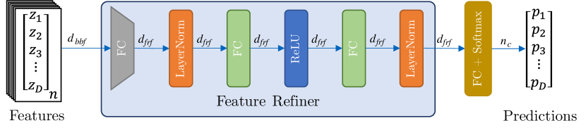
Figure 1: Feature Refiner architecture. Our network takes the features extracted by the backbone network. We apply dimension-reduction to reduce the model parameters followed by a symmetric 2-layered multi-layer perceptron.

2 Methodology

We propose a simple yet effective framework for improving the generalization from a small amount of data. In our work, we bring back fully-connected layers at the end of CNN-based architectures. We show that by adding as little as $0.37\%$ extra parameters during training, we can significantly improve the generalization in the low-data regime. Our network architecture consists of two main parts: a convolutional backbone network and our proposed Feature Refiner (FR) based on multi-layer perceptrons. Our method is task and model-agnostic and can be applied to many convolutional networks.

In our method, we extract features with the convolutional backbone network. Then, we apply our FR followed by a task-specific head. More precisely, we first reduce the feature dimension $d_{bbf}$ to $d_{frf}$ with a single linear layer to reduce the number of extra parameters. Then we apply a symmetric two-layer multi-layer perceptron wrapped around by normalization layers. We present the precise architecture of our Feature Refiner in Figure 1.

2.1 Online Joint Knowledge Distillation

One could argue that using more parameters can improve the performance just because of the increased expressivity of the network. To disprove this argument, we develop an online joint knowledge distillation (OJKD) method. Our OJKD enables us to use the exact same architecture as our baseline networks during inference and utilizes our FR solely during training.

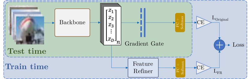
Figure 2: Online Joint knowledge distillation pipeline. Besides the baseline network’s classification head, we append an extra head with our Feature Refiner. The network is trained with the composed of the two heads’ cross-entropy loss. During training, the gradients coming from the single fully-connected layer are blocked. As a result, the backbone is updated only by the second head with our Feature Refiner. In test time, this extra head can be neglected without any noticeable performance loss.

We base our training pipeline on the baseline network’s architecture. We split the baseline network into two parts, the convolutional backbone for feature extraction and the final fully-connected classification head. We append an additional head with our Feature Refiner. We devise the final loss as the sum of the two head’s losses, making sure both heads are trained in parallel (online) and enforcing that they share the same network backbone (joint). During inference, we drop the additional head and use only the original one, resulting in the exact same test time architecture as our baseline. In other words, our FR head is the teacher network that shares the backbone with the student original head, and we distill the knowledge of the teacher head into the student head.

However, the key ingredient of our OJKD is the gradient-gating mechanism; we call it Gradient Gate (GG). This gating mechanism blocks the gradient of the original head during training, making the backbone only depend on our FR head. We implement this functionality with a single layer. During the forward pass, GG works as identity and just forwards the input without any modification. However, during the backward pass, it sets the gradient to zero. This way, the original head’s gradients are backpropagated only until the GG. While the original head gets optimized, it does not influence the training of the backbone but only adapts to it. Consequently, the backbone is trained only with the gradients of our FR head. Furthermore, the original head can still fit to the backbone and reach a similar performance as the FR head. We find that we can still improve upon the baseline without our gating mechanism but reach lower accuracy than when we use it. We show the pipeline of our OJKD in Figure 2.

3 Experiments

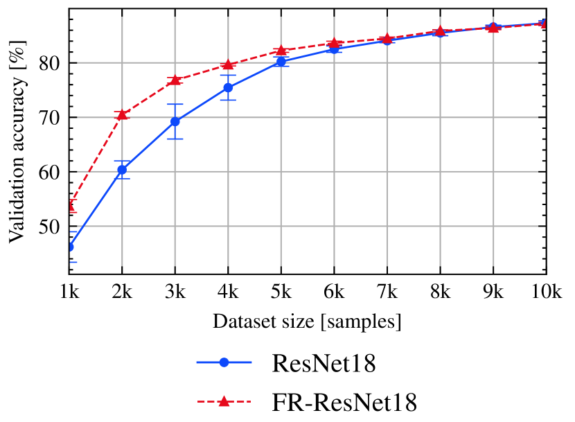
(a) CIFAR10

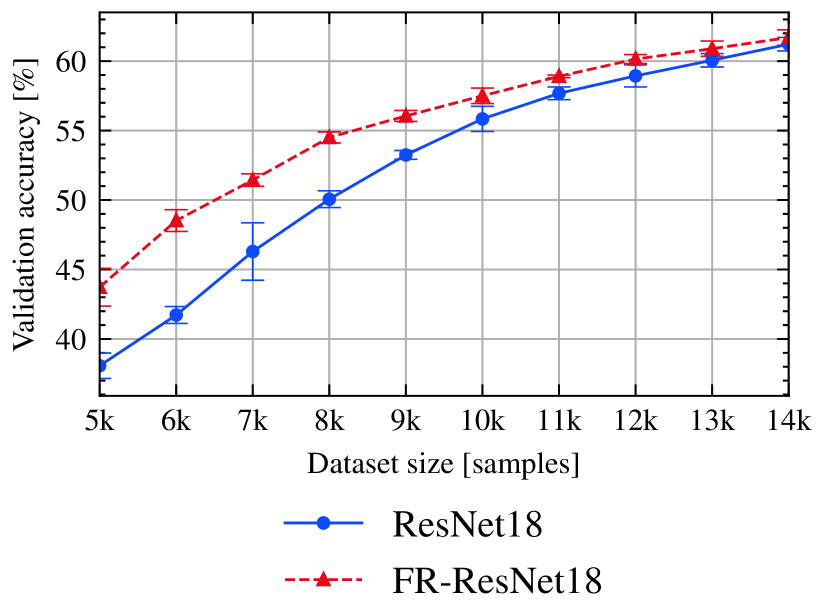
(b) CIFAR100

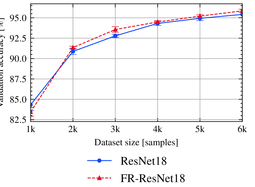
(c) Caltech101

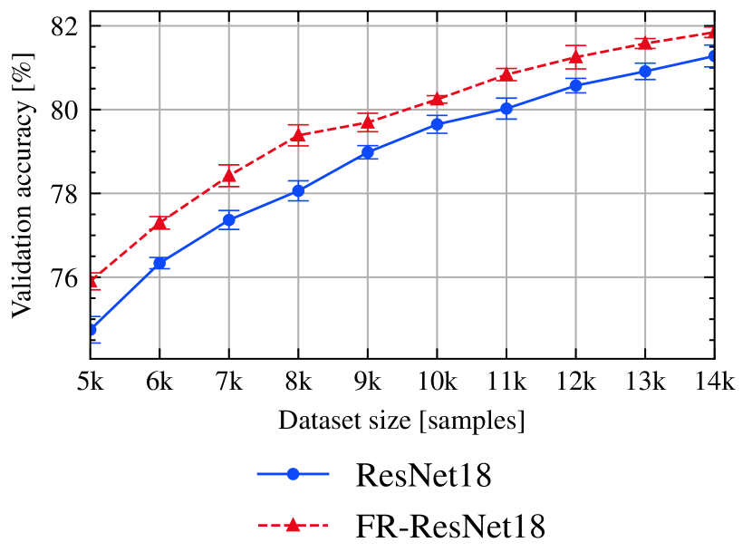
(d) Caltech256

Figure 3: Comparisons with ResNet18. We compare our approach (FR) to the baseline network ResNet18 in supervised learning. Our method significantly outperforms the baseline, especially in the more challenging earlier stages, when we have a small amount of data.

In this section, we demonstrate the substantial effectiveness of our simple approach improving the performance of neural networks in low-data regimes.

Datasets and the number of labels. For all experiments, we report accuracy as the primary metric and use four public datasets: CIFAR10 [18], CIFAR100 [18], Caltech101 [19], and Caltech256 [19]. We use the predefined train/test split for the CIFAR datasets, while we split the Caltech datasets into $70\%$ training and $30\%$ testing, maintaining the class distribution. In the simpler datasets, CIFAR10 and Caltech101, we start with an initial labeled pool of $1000$ images, while in the more complicated, CIFAR100 and Caltech256, we start with $5000$ labeled images. In both cases, we incrementally add $1000$ samples to the labeled pool in each cycle and evaluate the performance with the larger and larger training datasets. We use the active learning terminology for a’ cycle’, where a cycle is defined as a complete training loop.

CNN backbones. For most experiments, we use ResNet18 [8] as our backbone ($d_{bbf}=512$), and reduced feature size $d_{frf}=64$. We compare the results of our method with those of pure ResNet18 on both the supervised and active learning setups. Note that the supervised case (Figure 3) is equivalent to a random labeling strategy in an active learning setup. We compare our method with various active learning strategies. We also compare to a non-convolutional network, the MLPMixer [14]. Finally, to show the generability of our method, we also experiment with other backbone networks: ResNet34, EfficientNet, and DenseNet. We run each experiment $5$ times and report the mean and standard deviation. We train each network in a single GPU. We summarize the results in plots and refer to our supplementary material for exact numbers and complete implementation details.

Training details. For the CIFAR experiments, we follow the training procedure of [20]. More precisely, we train our networks for $200$ epochs using SGD optimizer with learning rate $0.1$, momentum $0.9$, weight decay $5e{-}4$, and divide the learning rate by $10$ after $80\%$ epochs. We used cross-entropy loss as supervision. For the more complex Caltech datasets, we start with an Imagenet-pre-trained backbone and reduce the dimensionality in our FR only to $256$. We use the same training setup for a full fine-tuning, except that we reduce the initial learning rate to $1e{-}3$ and train for only $100$ epochs.

3.1 Supervised Learning

Comparisons with ResNet18 [8]. We compare the results of our method with those of ResNet18. As shown in Figure 3(a), on the first training cycle ($1000$ labels), our method outperforms ResNet18 by $7.6$ percentage points (pp). On the second cycle, we outperform ResNet18 by more than $10pp$. We keep outperforming ResNet18 until the seventh cycle, where our improvement is half a percentage point. For the remaining iterations, both methods reach the same accuracy.

On the CIFAR100 dataset (see Figure 3(a)), we start outperforming ResNet18 by $5.7pp$, and in the second cycle, we are better by almost $7pp$. We continue outperforming ResNet18 in all ten cycles, in the last one being better by half a percentage point. We see similar behavior in Caltech101 (see Figure 3(c)) and Caltech256 (see Figure 3(d)).

A common tendency for all datasets is that with an increasing number of labeled samples, the gap between our method and the baseline shrinks. Therefore, dropping the fully-connected layers in case of a large labeled dataset does not cause any disadvantage, as was found in  [6]. However, that work did not analyze this question in the low-data regime, where using FC layers after CNN architectures is clearly beneficial.

Comparisons with MLPMixer [14] and ViT [12]. We also compare the results of our method with that of two non-convolutional networks, the MLPMixer and ViT. Similar to us, the power of MLPMixer is on the strengths of the fully-connected layers. On the other hand, ViT is a transformer-based architecture. Each Transformer block contains an attention block and a block consisting of fully-connected layers. Unlike these methods, our method uses both convolutional and fully-connected layers to leverage the advantages of both the high-level convolutional features and the global interrelation from the fully-connected layers. In Figure 4(a), we compare to MLPMixer and ViT on the CIFAR10 dataset. On the first cycle, we outperform MLPMixer by $4.4pp$ and ViT by circa $6pp$. We keep outperforming both methods in all other cycles, including the last one where we do better than them by circa $13pp$. As we can see, MLPMixer and ViT do not perform well even in the latest training cycles and require to be trained on massive datasets. We show a similar comparison for CIFAR100 in Figure 4(b).

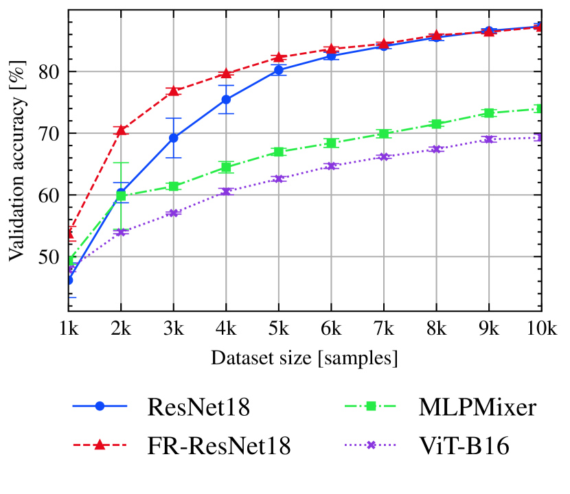
(a) CIFAR10 test accuracy.

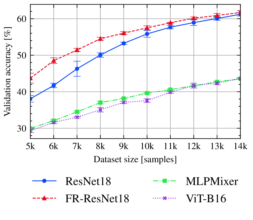
(b) CIFAR100 test accuracy.

Figure 4: Comparison with MLPMixer [14] and ViT. [12] We compare our method with MLPMixer and ViT. on the CIFAR10 (4(a)) and on the CIFAR100 (4(b)) datasets. Our method significantly outperforms both architectures in the low-data regime.

Comparisons with Knowledge Distillation baselines. To show that our method’s main strength comes from our FR head, we compare to several knowledge distillation (KD) methods. DML [21] trains two networks in an online KD setting. KDCL [22] aims to improve the generalization ability of DML by treating every network as students and training them to match the pooled logit distribution. Finally, KD [23] is the original offline method, which trains a teacher network, then distills its knowledge into a student. In each experiment, the teacher network is ResNet50, the student is ResNet18. As can be seen in Figure 5, our method significantly outperforms the KD methods, by up to 8.5pp on CIFAR10 and 3.6pp on CIFAR100 in the second iteration. In the later iterations, when more data is available and our approach converged to the baseline network’s performance, we start to see the benefit of the other KD methods. However, while our method comes with only $0.37pp$ extra parameters during training, the other KD methods use $210.5pp$ more parameters.

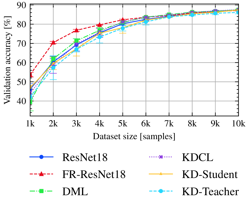
(a) CIFAR10

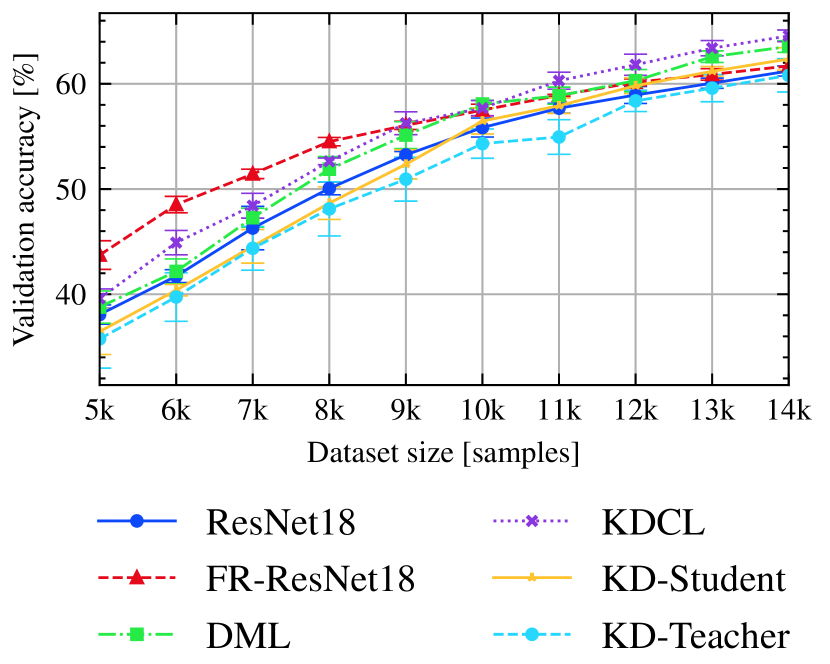
(b) CIFAR100

Figure 5: Comparisons with Knowledge Distillation baselines. We compare to several KD methods. Our method outperforms the baselines in the earlier iterations with a large margin.

Comparison with SimSiam [24]. Similarly to our method, SimSiam [24] uses a stop-gradient technique. They train a feature extractor in a self-supervised setting, then fine-tune a classifier head in a supervised setting. While SimSiam [24] can also be directly trained on smaller datasets, its behavior on the low data-regime has not been investigated yet. We compare our method against the CIFAR10 version of SimSiam on our datasplits and evaluate its performance with a kNN and with a linear classifier. The training scheme follows SimSiam [24], Appendix D. As it can be seen in Figure 6, our method significantly outperforms SimSiam [24] in all data splits by a maximum margin of $25.45pp$ in the second iteration, and by $8pp$ in the last iteration.

3.2 Active Learning

We put our method to the test under a typical low-data setting, active learning, where instead of randomly choosing samples to label, we choose them based on an acquisition score. The results in Section 3.1 can be considered a special case of active learning with a random acquisition score. We use maximum entropy acquisition score with our network and compare it with plain ResNet18 with maximum entropy and two state-of-the-art active learning methods, LLAL [20] and core-set [25].

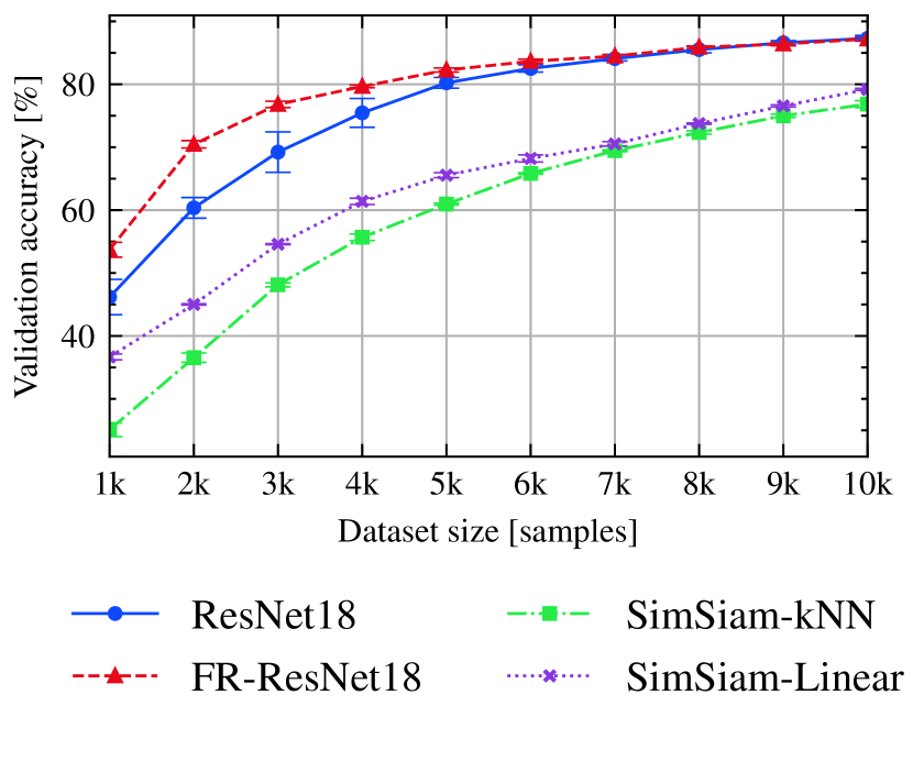
Figure 6: Comparison with SimSiam [24]. We compare our method against the CIFAR10 version of SimSiam [24]. Our method significantly outperforms SimSiam in the low-data regime.

In Figure 7, we summarize the results on all four datasets, showing our method’s superior performance. On CIFAR10, we outperform all methods in early cycles by a large margin, up to $7.3pp$ compared to the core-set approach in the second cycle. As more labels become available during training, all the methods tend to converge to the same result. A similar trend can be observed on the CIFAR100 dataset. Here, our approach achieves $5.2pp$ better accuracy in the second cycle. On the Caltech101 dataset, we have a slight advantage ($<0.5pp$) compared with the vanilla ResNet18. We have a larger advantage on the Caltech256 dataset, where we tend to outperform the second-best method by $1-1.5pp$. Furthermore, note that core-set and LLAL approaches perform much worse on these more complex datasets. The final gap between the maximum entropy acquisition and LLAL is $4.5pp$ on the Caltech256 and $1.4pp$ on the Caltech101 dataset.

3.3 Semi-Supervised Learning

We now do an experiment where we present preliminary results in semi-supervised learning. We choose to couple MixMatch [26] with our method and compare it with the original version of MixMatch. We use ResNet18 for the experiment and train the methods using only $250$ labels. MixMatch reaches $91.07$ accuracy, while our method reaches $91.56$ accuracy, improving by half a percentage point, and showing that our method can be used to improve semi-supervised learning.

3.4 Backbone Agnosticism

We check if our method can be used with other backbones than ResNet18. We show the results for ResNet34, DenseNet121, and EfficientNetB3 on CIFAR10 and CIFAR100 in Figure 8. The goal of the experiment is to show that our method is backbone agnostic and generalizes both to different versions of ResNet as well as to other types of convolutional neural networks. As we can see, our method significantly outperforms the baselines on both datasets and for all three types of backbones.

3.5 Ablation

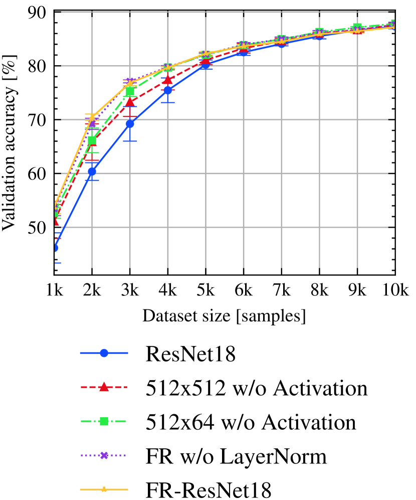
(a) Feature Refiner

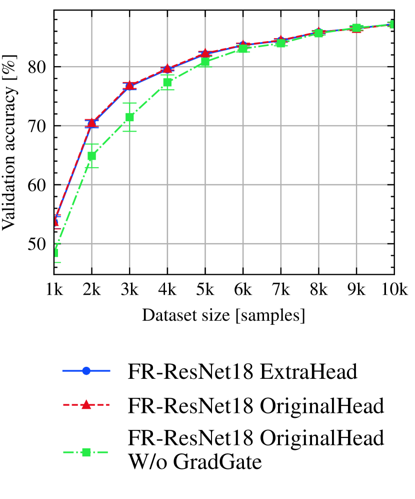
(b) OJKD ablation

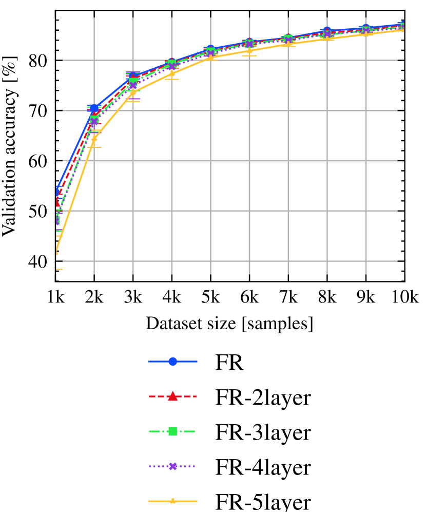
(c) Number of layers ablation

Figure 9: Feature Refiner 9(a): We apply parts of our Feature Refiner step-by-step. First, we use only a single linear layer without any extra activation (512x512 w/o Activation), then apply our dimension reduction step (512x64 w/o Activation). Finally, we evaluate the effect of the LayerNorm layer. OJKD ablation 9(b): Our online joint knowledge distillation enables us to utilize the advantages of our Feature Refiner without increasing the number of model parameters at the same time. Our method also helps even without the Gradient Gate. Number of layers ablation 9(c): We study the effect of the number of nonlinear fully-connected layers. More layers do not lead to better performance.

Feature Refiner We conduct a detailed ablation of the architecture of our Feature Refiner, showing the effect of the specific elements. We start with the backbone ResNet18 and build our Feature Refiner up step-by-step. Figure 9(a) shows the results on the CIFAR10 dataset. First, we apply only a single linear layer without any activation function before the output layer (512x512 w/o Activation). Interestingly, we can already see a great improvement of $4.9pp$ in the first cycle, reaching $5.5pp$ in the second cycle. Second, we change the previously applied linear layer to reduce the dimension, as we did in our Feature Refiner (512x64 w/o Activation). This step further improves the results up to $2.3pp$ in the third cycle. Third, we add our fully-connected layers with the ReLU activation (FR w/o LayerNorm), which yields an improvement of $3.1pp$ in the second cycle. Finally, we use our complete architecture by applying the normalization layers, reaching the best results in the earlier stages, giving an additional performance boost of $1.2pp$ in the second stage.

Online joint knowledge distillation We now evaluate our proposed OJKD. In these experiments, we highlight that during inference, we can drop the Feature Refiner head without any noticeable performance loss. We use the same training strategy as described in Section 2.1. We train together with the original and Feature Refiner heads. However, during inference, we evaluate both heads. In Figure 9(b) we show both heads’ performance on the CIFAR10 dataset. As we can see, both heads have barely distinguishable performance, showing that the knowledge of our teacher FR head can be properly distilled into the student original head. Furthermore, we ablate the effect of our proposed Gradient Gate. Without our gating mechanism, we can still improve upon the baseline up to $4.5pp$, but using it can give us a further $5.6pp$ improvement in the second stage.

The effect of the number of layers. We now study the number of layers with nonlinearities. To do so, we add nonlinear layers in our Feature Refinement. We show the results on the CIFAR10 dataset in Figure 9(c). As we can see, adding more nonlinear layers comes with a decrease in performance. In fact, the more layers we add, the larger is the decrease in performance compared to our original model. This makes sense considering that by increasing the number of layers, we increase the number of learnable parameters, and thus we might cause overfitting.

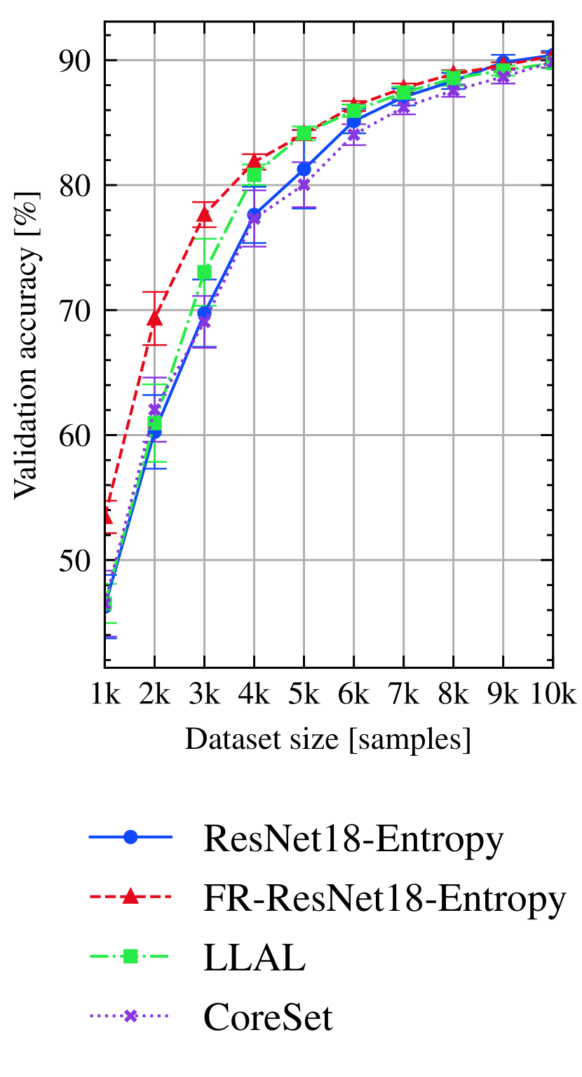
(a) CIFAR10

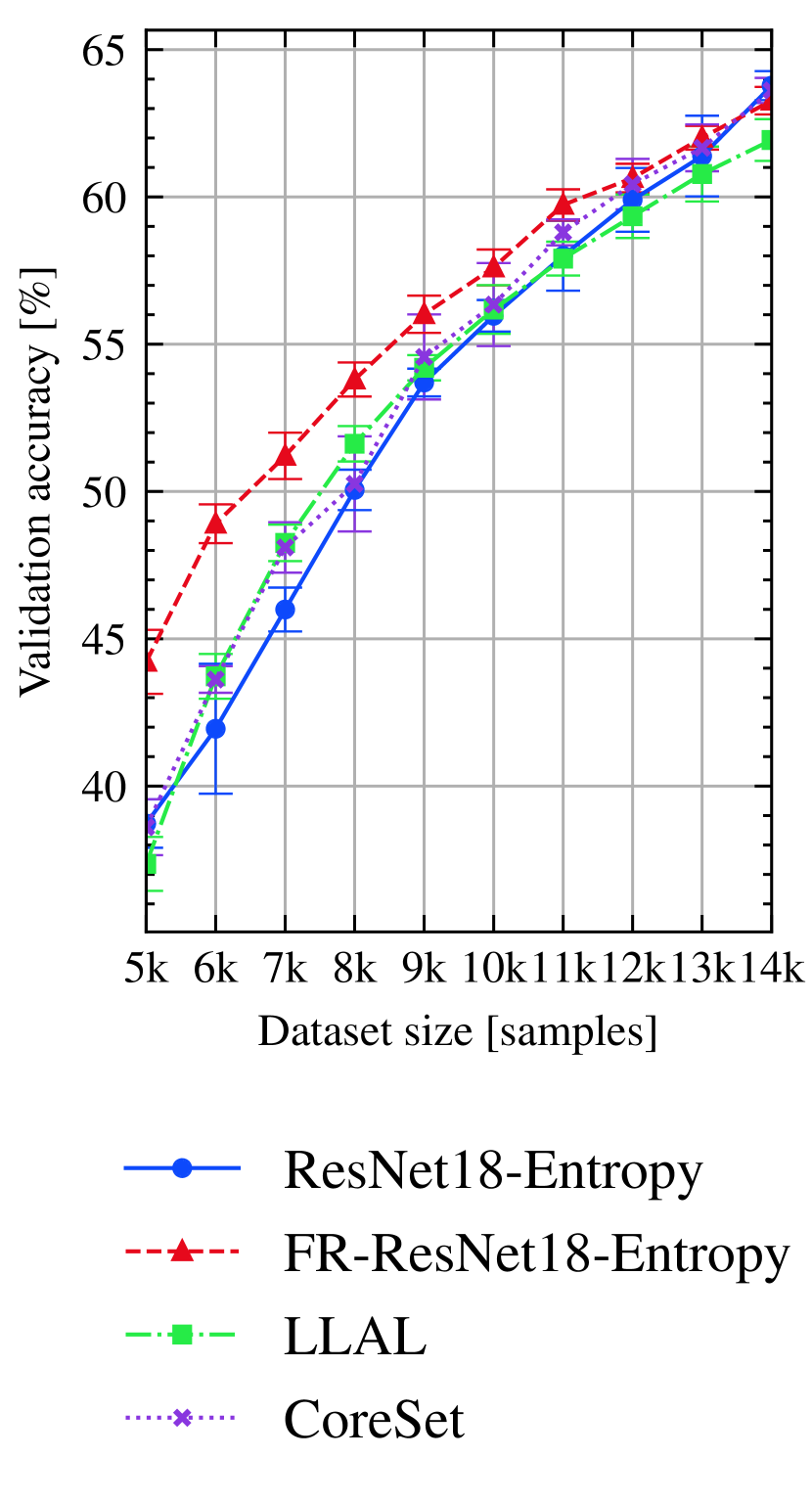
(b) CIFAR100

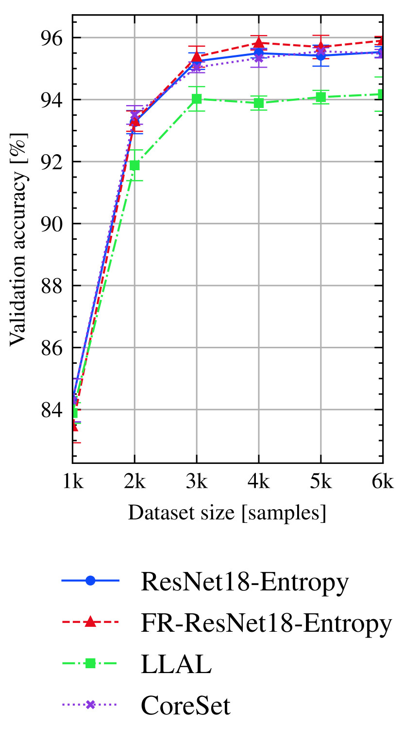
(c) Caltech101

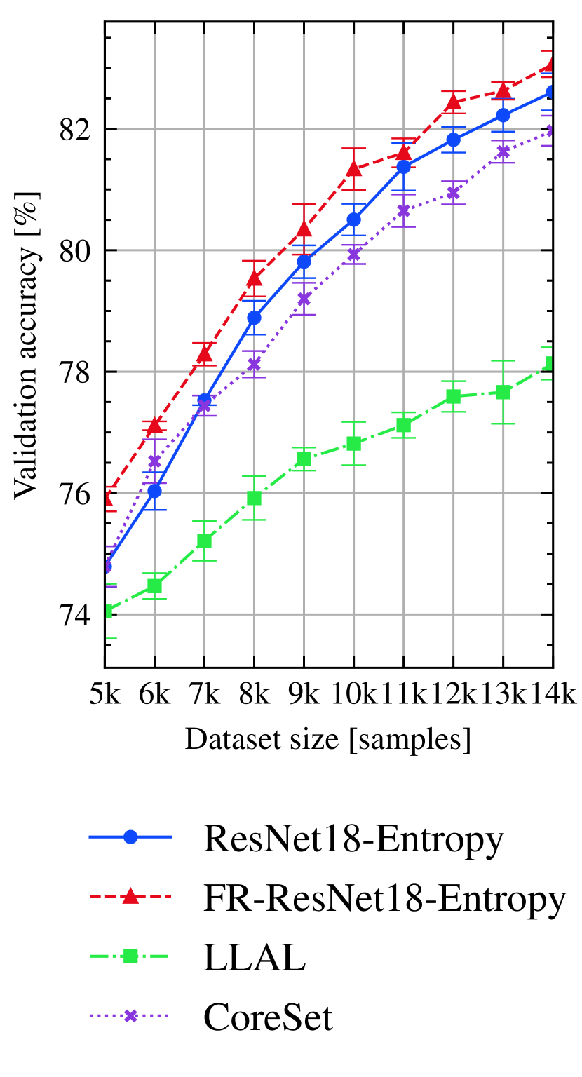
(d) Caltech256

Figure 7: Active Learning. We compare our approach (FR) in an active learning setup based on maximum entropy. We compare with ResNet18 using entropy-based acquisition score, LLAL, [20] and core-set [25]. Our method significantly outperforms all others, especially in the more challenging earlier stages, when we have a small amount of data.

4 Related Work

All-convolutional networks. Convolutional neural networks [1, 2] have made a breakthrough in many computer vision tasks since the pioneering work of [4]. Other works [27, 5] improved over those architectures, typically by increasing the number of convolutional layers but by keeping the same architecture: many convolutional and pooling layers followed by a few fully-connected layers. However, this design choice was questioned in the famous Striving for simplicity [6] paper, where it was argued that there is no need for fully connected layers. Fully convolutionized architectures such as Google-Inception [7] or ResNets [8] followed, significantly outperforming the previous state-of-the-art. Some more recent works typically tended to improve the architecture of ResNet architectures either by enlarging the number of convolutional filters [8] or densely connecting convolutional layers [10]. Probably the best solution was found in the EfficientNet [28], which simultaneously increases the image resolution, number of convolutional channels, and number of convolutional layers. A constant of these approaches is that they completely get rid of the fully connected layers. Contrary to them, we find out that adding fully-connected layers comes with a massive benefit in performance when the number of labeled points is limited. By doing so, we are able to improve the performance of several backbones in different learning tasks.

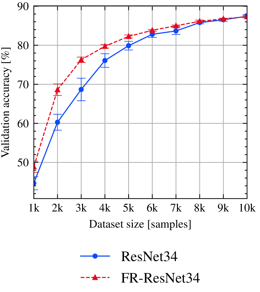
(a) ResNet34-CIFAR10.

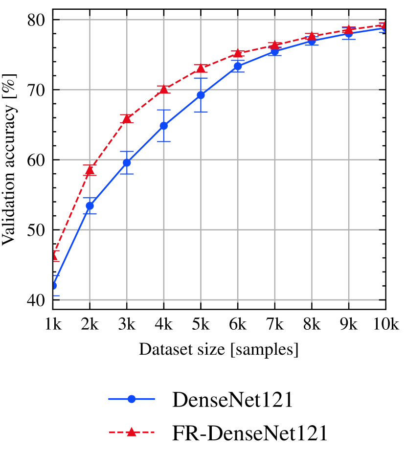
(b) DenseNet121-CIFAR10.

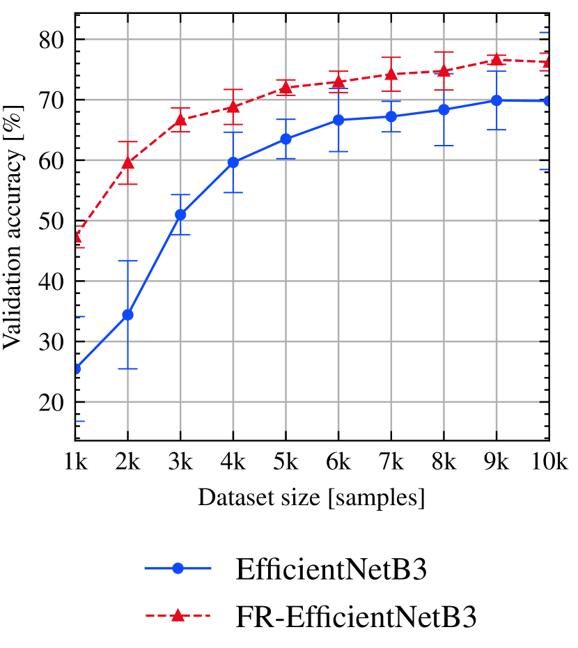
(c) EfficientNetB3-CIFAR10.

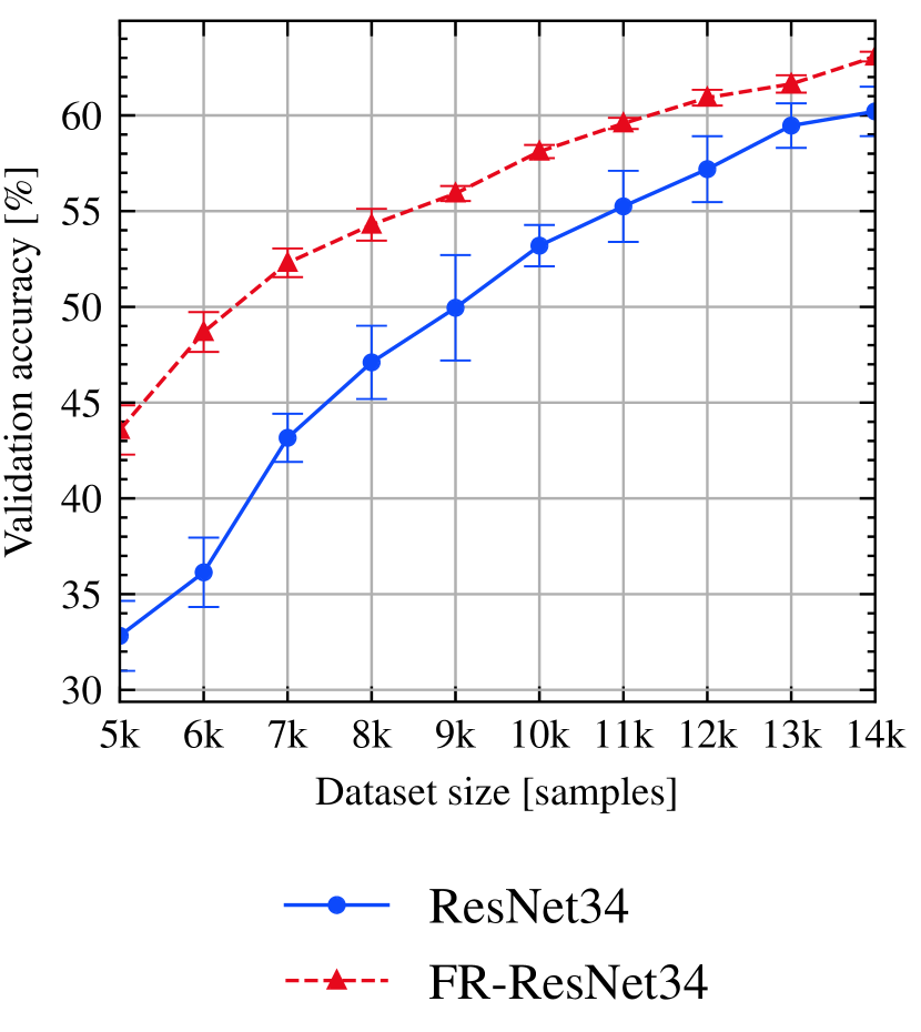
(d) ResNet34-CIFAR100.

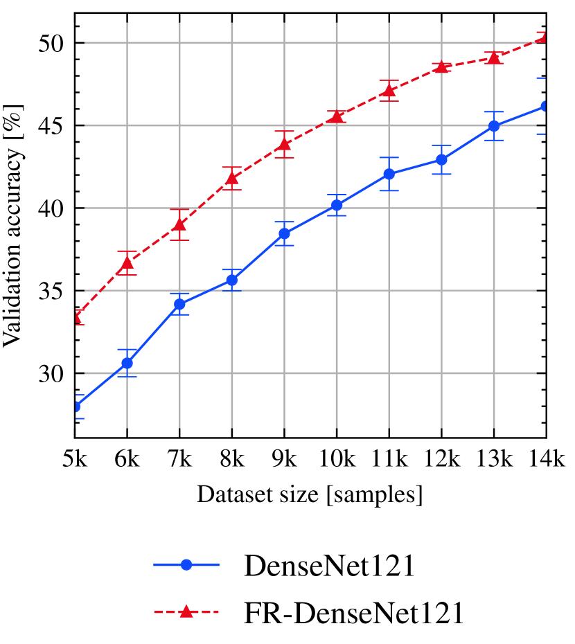
(e) DenseNet121-CIFAR100.

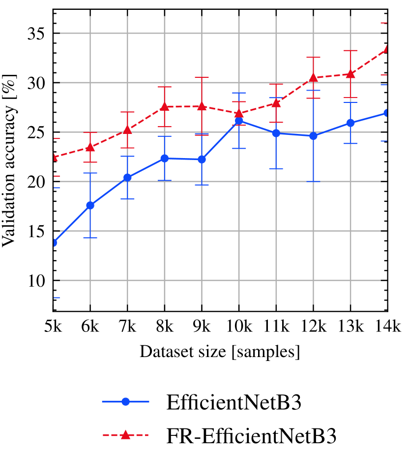
(f) EfficientNetB3-CIFAR100.

Figure 8: Backbone agnosticism. We show that our approach is agnostic to the backbone. We evaluate our approach on the CIFAR10 and CIFAR100 datasets with ResNet34, DenseNet121, and EfficientNet-B3 backbones. In all cases, our method significantly improves over the original network.

Non-convolutional networks. A parallel line of research has shown that convolutional neural networks can be replaced either by vision transformers [12, 13] or multi-layer perceptrons [14, 15, 16]. The main idea behind these works is to leave the network as much freedom as possible during the learning procedure instead of injecting inductive bias into the network. Indeed, in multi-layer perceptrons, every unit is connected to all the units in both the previous and the next layer, allowing it to use all the information of the proceeding layer as well as pass it into the next one. Works like MLPMixer [14] and others have shown promising results in several vision tasks. Still, they come with a series of limitations, such as the need for pre-training on very large datasets and requiring a massive amount of computational resources. Our work is similar to MLPMixer [14] in the sense that we also leverage the power of multi-layer perceptrons to solve different vision tasks. However, unlike them, we do not get rid of the convolutional layers, but we advocate for hybrid networks. Our networks do not need pre-training and massive computational resources, while it manages to significantly improve state-of-the-art results when trained with a limited number of labeled points.

Knowledge distillation. With the advancements in computational power, larger neural networks are possible to train. However, effective neural networks are required during inference in many practical applications, especially mobile or embedded applications. This requirement motivates the field of Knowledge Distillation (KD). The goal of KD is to reduce the computational demand of a trained network’s inference by maintaining its performance. This could be in the form of offline distillation, where one network is used as a teacher to distill its knowledge into another smaller network, the student [23]. However, online distillation has gained more attention lately, thanks to its simpler pipeline [29]. In such a setup, the student and teacher models are trained together end-to-end. For more details on this field, we refer to the work of Gou et al. [29] The published online distillation methodologies are mainly specifically applied for ensemble distillation [30]. On the contrary, we propose an effective yet general online distillation method. We attach a separate head during the training (the Feature Refiner) while using a gating mechanism that blocks the gradients coming from the original softmax layer of the network. On inference, we can simply drop the Feature Refiner head without noticeable performance drop, thus, using no extra parameters.

Stop-gradient. SimSiam [31] and BYOL [32] train two branches jointly in a self-supervised setting with different augmentations. In BYOL, the target is provided by the averaged version of the main network, while in SimSiam the same network is used with the stop-gradient technique. These methods share similarities with our OJKD; however, they cannot be directly applied to supervised learning, and they are trained on large datasets. Instead, we focus on generalization from a low amount of data in a supervised setting.

5 Conclusion

In this paper, we question the long-believed idea that convolutional neural networks do not need fully-connected layers. Perhaps surprisingly, we show that using hybrid networks that use both convolutional high features and interrelations coming from fully-connected layers improves the generalization performance in the low-data regime, without any drawback in the high-data regime. To show a fair comparison, we also introduce a gating mechanism that allows distilling the knowledge from our extra head with the added FC layers to the baseline network. We show that our approach is model agnostic by evaluating different backbone networks. We show in our experiments that our method yields a significant improvement over the state-of-the-art in supervised and active learning, in a wide range of standard classification datasets without an increase in the number of used parameters.

Broader Impact / Limitations

A shortcoming of our method is that we cannot improve the networks that already contain fully-connected layers, such as the VGG Network [5]. In the supplementary material, we do an experiment showing that our Feature Refiner cannot further improve VGG Network’s accuracy. However, we were able to decrease the number of learnable parameters by $67\%$.

Another deficiency of our paper is the lack of a theoretical explanation. Although the empirical results underline our methodology, we could not find any mathematical proof for it. Our speculative explanation is that if the network has only a single final layer, then the backbone’s feature space must be linearly separable. Our intuition is that in the case of a low amount of data, the convolutional layers do not get enough supervision to find the right local reasoning, which limits its flexibility. Having additional final fully-connected layers gives global supervision and increases the flexibility of the network to reach better optima. We note that the research in deep learning has been mostly head by empirical results. We believe that theoretical explanations are desirable and ultimately needed. At the same time papers without a clear (or a downright wrong) theoretical explanation have had a massive impact on deep learning, as is the case of the batch-normalization [33] paper. We hope that our work can open a new interesting line of research, and inspire other researchers to question the ’common knowledge’ in deep learning. Furthermore, it would be interesting to see if our results can be generalized in domains where the number of labeled data is very scarce, such as medical imaging.

Acknowledgements This work was supported by a Sofja Kovalevskaja Award, a postdoc fellowship from the Humboldt Foundation, the ERC Starting Grant Scan2CAD (804724), and the German Research Foundation (DFG) Research Unit "Learning and Simulation in Visual Computing".

The Unreasonable Effectiveness of Fully-Connected Layers for Low-Data Regimes
— Supplementary material —

peter-kocsis.github.io/LowDataGeneralization/

In this appendix, we start by providing more implementation details in Section A. In Subsection A.1, we detail the hyperparameters. In Subsection A.2, we give further information with regards to the used datasets. In Table 2, we show the number of extra parameters used during training with our method for all our experiments. In Subsection A.3, we provide the libraries used for the trainings of MLPMixer and ViT. In Subsection A.4, we provide more information for the Active Learning experiments.

In Section B, we do extra experiments with the VGG networks which already uses fully-connected layers. In Section C, we evaluate the robustness of our method on the CIFAR10-C dataset. Then, in section D, we evaluate our method on the Caltech101 dataset without any pretraining. Finally, in Section E, we provide the exact numbers (mean and standard deviation) for all the plots in the paper.

Appendix A Training details

A.1 Hyperparameters

Doing hyperparameter optimization in low-data regimes is extremely difficult. This is because in different cycles we have different datasets. Optimizing on them independently yields different optimal hyperparameters, which makes the results difficult to compare. Furthermore, that leads to several trainings for each cycle, which is costly. In addition, datasets like CIFAR and Caltech have public testing set, which means that an extensive hyperparameter optimization might lead to an overfitting of the testing set, and unreliable generalization results. To avoid all these issues, we decide to follow the work of LLAL [20] and use a single hyperparameter set across all the experiments and comparison. More details about the datasets and the used hyperparameters can be found in Table 1

Table 1: Summary of the used datasets and specific hyperparameters. The first block until the dashed line describes the datasets. The second block shows the used data augmentations, followed by the training hyperparameters. During learning rate scheduling, we divide the learning rate by $10$ after $80\%$ epochs.

	CIFAR10	CIFAR100	Caltech101	Caltech256
Number of classess	10	100	102	257
Number of training samples	50000	50000	6117	21531
Number of test samples	10000	10000	2560	9076
Official test split	✓	✓	✗	✗
Image size	32x32	32x32	Various	Various
Class balance	✓	✓	✗	✗
Random horizontal flip	✓	✓	✓	✓
Random crop	32x32, p=4	32x32, p=4	224x224, p=16	224x224, p=16
Normalization	✓	✓	✓	✓
Size of initial labeled pool	1000	5000	1000	5000
Samples labeled in stage	1000	1000	1000	1000
Number of stages	10	10	6	10
Feature size	64	64	256	256
Optimizer	SGD	SGD	SGD	SGD
Learning rate	0.1	0.1	0.001	0.001
Learning rate scheduler	✓	✓	✓	✓
Momentum	0.9	0.9	0.9	0.9
Weight decay	5e-4	5e-4	5e-4	5e-4
Number of epochs	200	200	100	100

A.2 Datasets and the number of labels.

For all supervised experiments, we use the same pre-defined datasplits. We obtained the datasplits with incremental random sampling. This ensures that the comparisons are fair, and subject to only the network architecture. Doing otherwise might result with some method being favored by having a better training split.

A.3 MLPMixer [14] and ViT [12].

MLPMixer [14] and ViT [12] were originally developed for ImageNet. In order to achieve their best performance we compared multiple architectures specifically tailored for the CIFAR datasets, and chose the best performing ones, specifically, MLPMixer-Nano [24] and ViT-CIFAR10 [34]

A.4 Active Learning.

To achieve comparable results, we closely followed the active learning setup of LLAL [20]. We split the dataset into two parts: labeled and unlabaled pool. During training, we access only the labeled pool. In each cycle, we train a model on the labeled pool and use its predictions on the unlabeled pool to select samples to be included in the labeled pool for the next cycle. In each cycle, we reinitialize the model weights.

During the experiments, we noted that there is a difference between our and the officially reported LLAL [20] results. We found that the reason behind that is the mismatch between their and our PyTorch versions. They used PyTorch 1.1, while we use more modern PyTorch 1.7. Downgrading to the older version yields comparable results to the published ones. While we believe that reproducibility and comparability is crucial in research, using outdated libraries is not an ideal solution. Consequently, we compare their method and ours using PyTorch 1.7. We think that this is both fair, and allows an easier reproducibility for future research.

Table 2: Extra parameters. Number of extra parameters used during training for all experiments.

	CIFAR	Caltech
ResNet18	11173962	11228325
FR-ResNet18	+42058 (0.38%)	+289893 (2.58%)
ResNet34	21282122	✗
FR-ResNet34	+42058 (0.20%)	✗
DenseNet121	6964096	✗
FR-DenseNet121	+74826 (1.07%)	✗
EfficientNetB3	10711602	✗
FR-EfficientNetB3	+82660 (0.77%)	✗

Appendix B VGG experiment

We conduct an experiment with an old-fashioned architecture that uses final fully-connected layers, the VGG11 [5]. Since this architecture follows our proposed solution, we are unable to improve upon its performance. However, we show that our light-weight Feature Refiner (FR) is able to achieve the same results, but using only $9,262,282$ parameters instead of $28,144,010$, resulting with a $67\%$ reduction in the number of weights. We present the results on Figure 10.

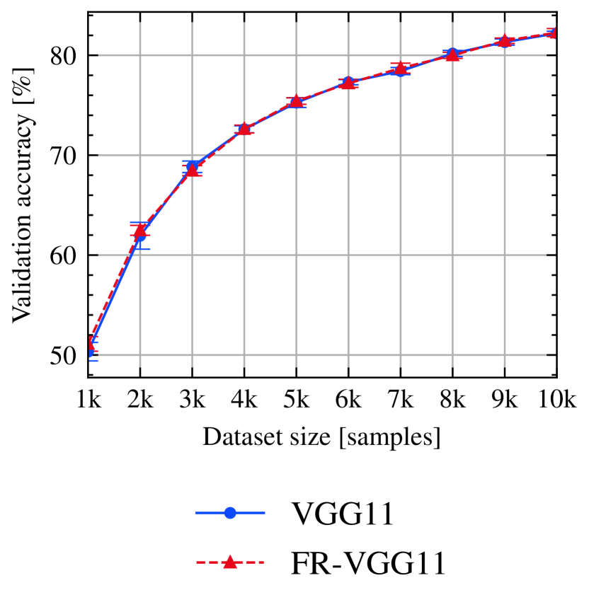
(a) CIFAR10 plot

#Samples	VGG11	FR-VGG11
1000	50.33$\pm$0.93	51.06$\pm$0.78
2000	61.94$\pm$1.34	62.43$\pm$0.47
3000	68.84$\pm$0.58	68.42$\pm$0.49
4000	72.60$\pm$0.35	72.62$\pm$0.35
5000	75.27$\pm$0.49	75.40$\pm$0.34
6000	77.31$\pm$0.26	77.17$\pm$0.44
7000	78.42$\pm$0.36	78.66$\pm$0.52
8000	80.18$\pm$0.31	79.98$\pm$0.32
9000	81.33$\pm$0.32	81.46$\pm$0.29
10000	82.21$\pm$0.20	82.22$\pm$0.44

(b) CIFAR10 numerical results

Figure 10: VGG experiment. We evaluate our method with the VGG architecture. We can achieve highly similar performance with $67\%$ fewer parameters.

Appendix C Robustness benchmark

We evaluate the robustness of ResNet18 and our model (FR-ResNet18) on the CIFAR10-C dataset [35]. CIFAR10-C contains a total of 95 perturbed test sets under $19$ different corruptions with $5$ severity levels. We present average results of $5$ independent runs (Figure 14) over the different severity levels (Figure 13) and over the different corruption types (Figure 13). Our method consistently outperforms the baseline in cases of lower corruption severity. In cases of higher corruption severity (severity 3 and severity 4), in the very low-data regime, our method significantly outperforms the baseline. However, with more added data, the baseline starts outperforming our method.

Appendix D Caltech without pre-training

Since the Caltech datasets are more complex, and also to show that our method works with pretrained models as well, we used Imagenet-pretrained backbone for the Caltech experiments in the main paper. Now, we conduct a minimal experiment to evaluate our method without pretraining. We run our method on the Caltech101 dataset without pretraining in the first three datasplits. As it can be seen in Figure 11, in the first cycle, we are worse than ResNet18 by $1pp$, similarly as with ImageNet pretraining, where the difference was 0.9pp. In the second cycle, we outperform ResNet18 by $0.7pp$, while with ImageNet pretraining we outperformed them by $0.5pp$. In the third cycle, we outperform ResNet18 by $1.4pp$, while with ImageNet pretraining we outperformed them by $0.8pp$. In this way, we show that while both ResNet18 and our method reach significantly lower results than when we use ImageNet pretraining, the relative improvement of our method compared to ResNet18 remains.

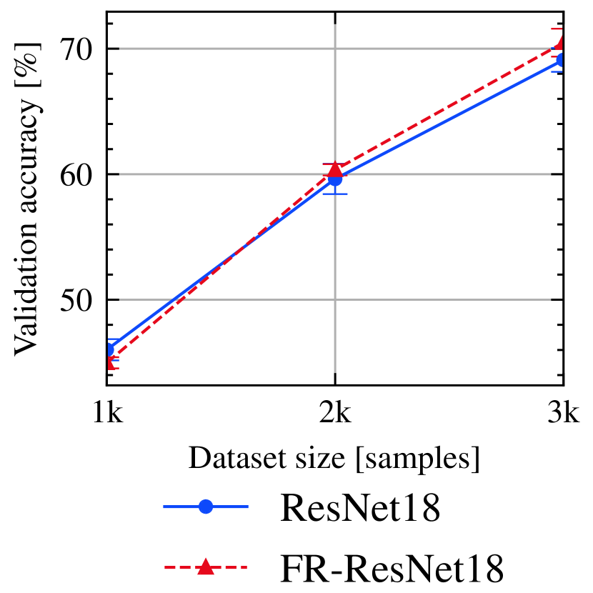
(a) Caltech101 plot

#Samples	ResNet18	FR-ResNet18
1000	46.02$\pm$0.85	44.98$\pm$0.45
2000	59.62$\pm$1.21	60.35$\pm$0.45
3000	69.10$\pm$0.95	70.48$\pm$1.11

(b) Caltech101 numerical results

Figure 11: Caltech101 w/o pretraining. We evaluate our method on the first three splits of the Caltech101 dataset without Imagenet-pretraining. While both ResNet18 and our method reach significantly lower results than when we use ImageNet pretraining, the relative improvement of our method compared to ResNet18 remains.

Appendix E Numerical results

In this section, we provide the exact numbers of all our results presented in the paper. Table 3, 4, 5, 6, 7, 8, 9 summarize the results provided in Figure 3, 4, 5, 6, 7, 8, 9. We provide the mean and standard deviation obtained by running the same experiment five times with different model initializations.

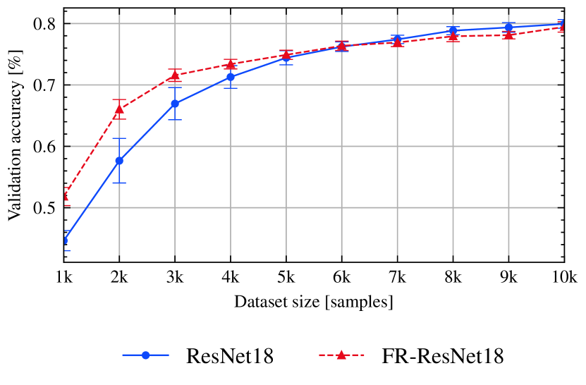
(a) Severity 0

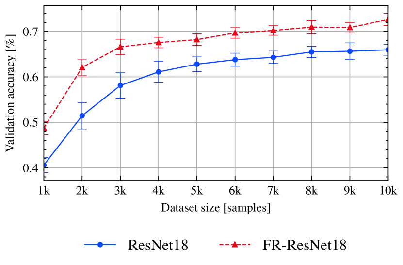
(b) Severity 1

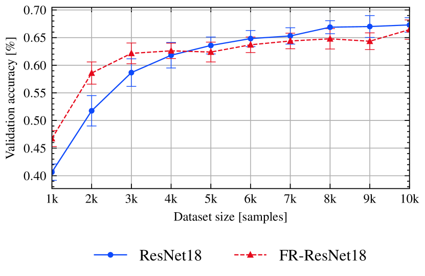
(c) Severity 2

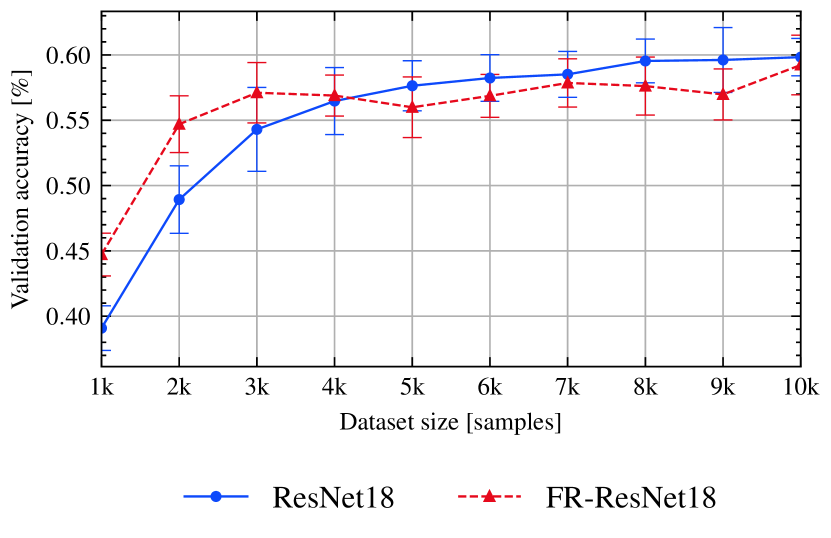
(d) Severity 3

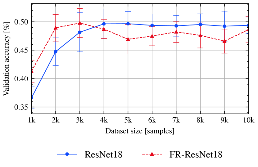
(e) Severity 4

Figure 12: Robustness benchmark - Severity. We evaluate the robustness of our method on the CIFAR10-C dataset. We present the average score for all severity levels. Our method consistently outperforms the baseline in cases of lower corruption severity. In cases of higher corruption severity (12(d) and 12(e)), in the very low-data regime, our method significantly outperforms the baseline. However, with more added data, the baseline starts outperforming our method.

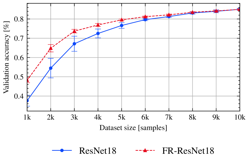
(a) Brightness

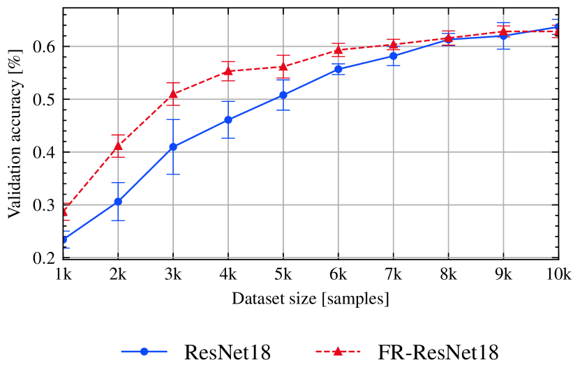
(b) Contrast

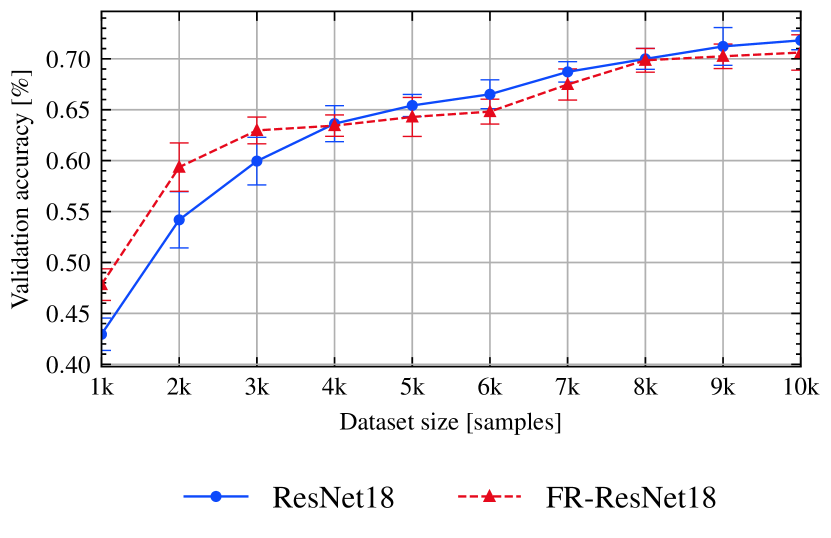
(c) Defocus Blur

(d) Elastic Transform

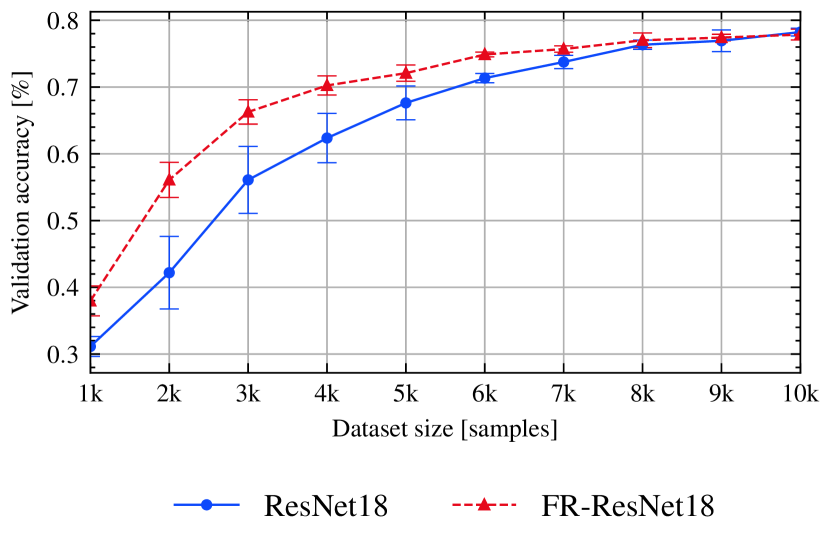
(e) Fog

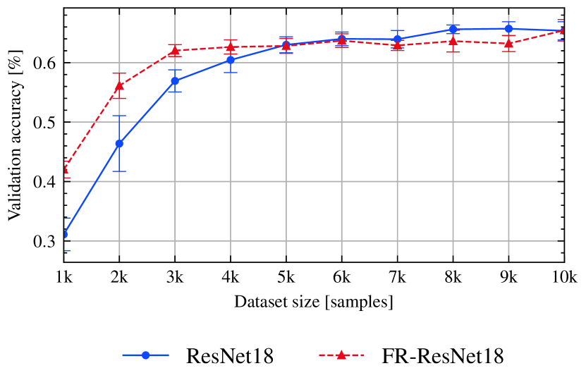
(f) Frost

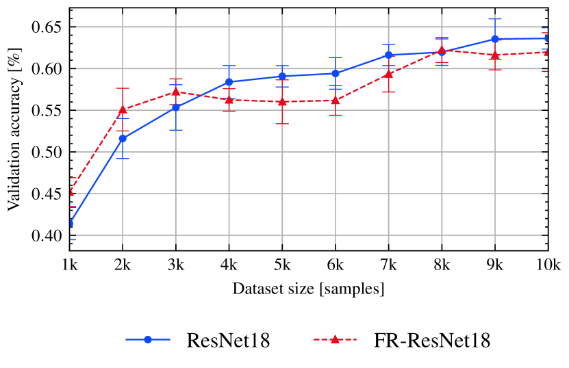
(g) Gaussian Blur

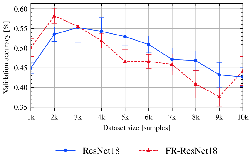
(h) Gaussian Noise

(i) Glass Blur

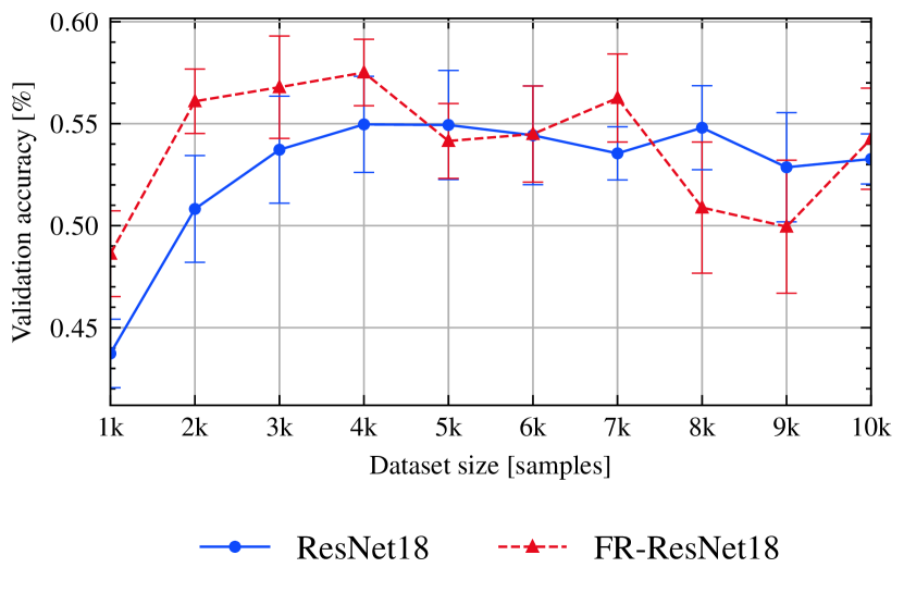
(j) Impulse Noise

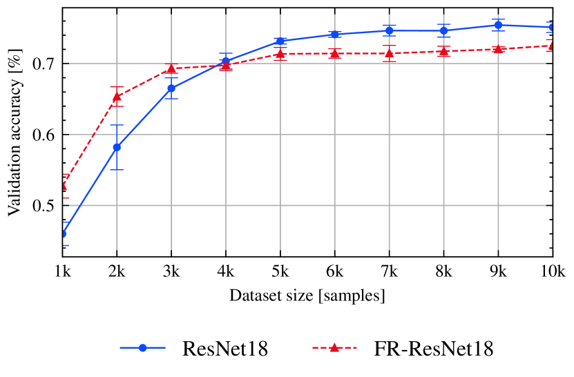
(k) JPEG Compression

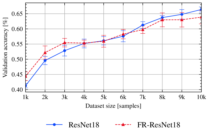
(l) Motion Blur

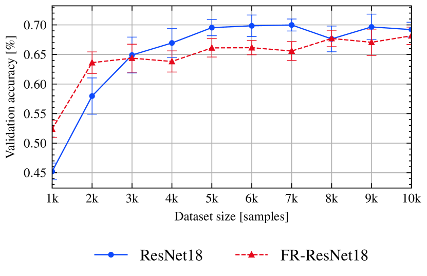
(m) Pixelate

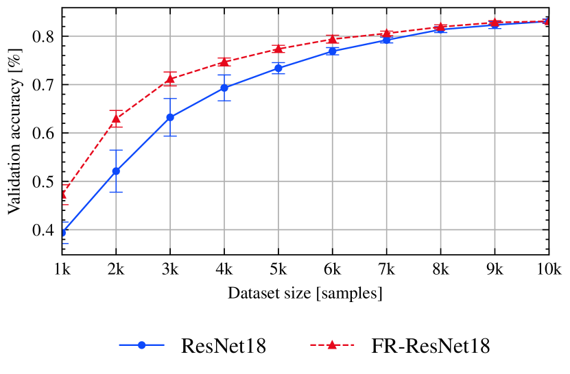
(n) Saturate

(o) Shot Noise

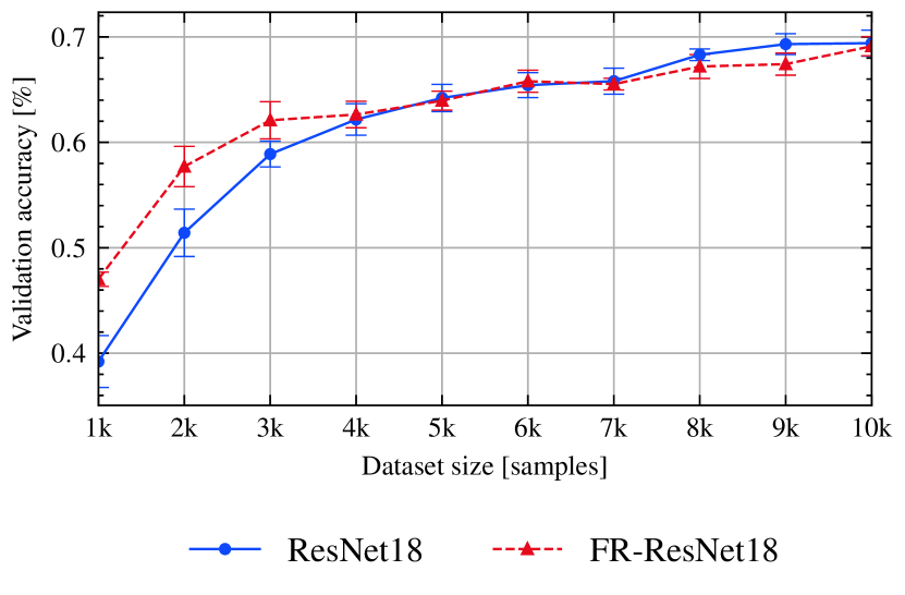
(p) Snow

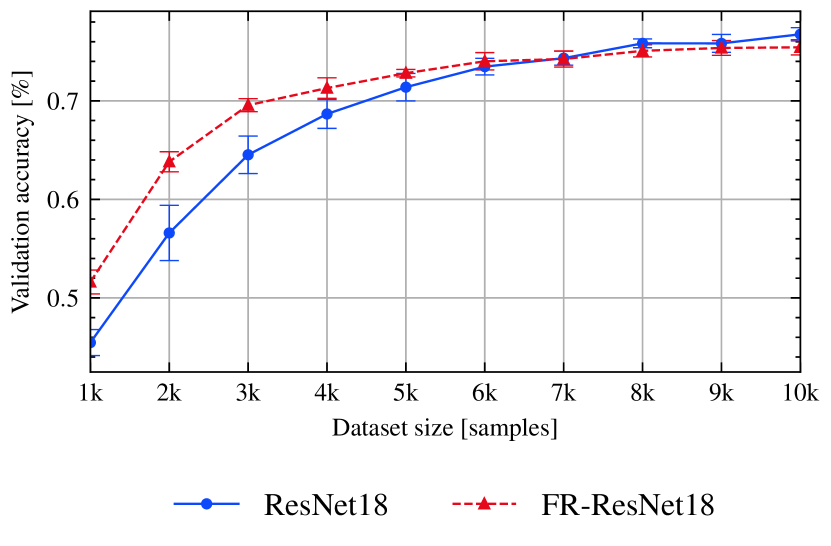
(q) Spatter

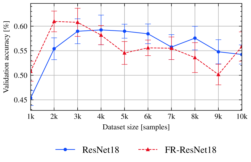
(r) Speckle Noise

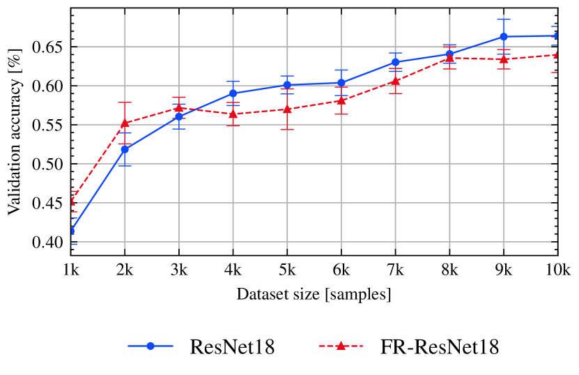
(s) Zoom Blur

Figure 13: Robustness benchmark - Corrpution types. We evaluate the robustness of our method on the CIFAR10-C dataset. We present the average score for all corruption types. Our method consistently outperforms the baseline in the earlier iterations.

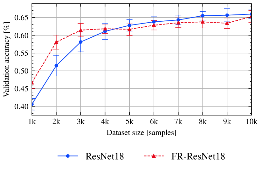
Figure 14: Robustness benchmark - Overall. We evaluate the robustness of our method on the CIFAR10-C dataset. We present the average score over all datasets. Our method performs better in the earlier iterations.

Table 3: Comparisons with ResNet18 [8]. We compare our approach to our main baseline network, to ResNet18 [8] on the CIFAR10, CIFAR100, Caltech101 and Caltech256 datasets in supervised learning. Our method significantly outperforms the baseline.

(a) CIFAR10

#Samples	ResNet18 [8]	FR-ResNet18
1000	46.18$\pm$2.81	53.70$\pm$1.18
2000	60.36$\pm$1.64	70.46$\pm$0.59
3000	69.22$\pm$3.21	76.81$\pm$0.50
4000	75.45$\pm$2.29	79.66$\pm$0.21
5000	80.23$\pm$0.85	82.27$\pm$0.33
6000	82.52$\pm$0.59	83.65$\pm$0.34
7000	84.08$\pm$0.38	84.48$\pm$0.26
8000	85.51$\pm$0.51	85.88$\pm$0.21
9000	86.59$\pm$0.34	86.42$\pm$0.31
10000	87.31$\pm$0.46	87.20$\pm$0.29

(b) CIFAR100

#Samples	ResNet18 [8]	FR-ResNet18
5000	38.07$\pm$0.92	43.73$\pm$1.36
6000	41.72$\pm$0.61	48.52$\pm$0.78
7000	46.29$\pm$2.07	51.44$\pm$0.45
8000	50.06$\pm$0.60	54.51$\pm$0.40
9000	53.25$\pm$0.32	56.06$\pm$0.40
10000	55.84$\pm$0.90	57.50$\pm$0.56
11000	57.68$\pm$0.46	58.90$\pm$0.09
12000	58.94$\pm$0.80	60.15$\pm$0.33
13000	60.06$\pm$0.48	60.89$\pm$0.55
14000	61.22$\pm$0.48	61.70$\pm$0.56

(c) Caltech101

#Samples	ResNet18 [8]	FR-ResNet18
1000	84.33$\pm$0.70	83.46$\pm$0.53
2000	90.87$\pm$0.38	91.34$\pm$0.17
3000	92.78$\pm$0.20	93.56$\pm$0.35
4000	94.31$\pm$0.25	94.49$\pm$0.17
5000	94.94$\pm$0.28	95.21$\pm$0.20
6000	95.42$\pm$0.38	95.86$\pm$0.21

(d) Caltech256

#Samples	ResNet18 [8]	FR-ResNet18
5000	74.75$\pm$0.32	75.90$\pm$0.20
6000	76.34$\pm$0.13	77.30$\pm$0.15
7000	77.37$\pm$0.23	78.42$\pm$0.26
8000	78.06$\pm$0.24	79.39$\pm$0.25
9000	78.98$\pm$0.16	79.69$\pm$0.22
10000	79.65$\pm$0.21	80.24$\pm$0.09
11000	80.02$\pm$0.25	80.84$\pm$0.15
12000	80.57$\pm$0.17	81.25$\pm$0.28
13000	80.91$\pm$0.20	81.58$\pm$0.12
14000	81.28$\pm$0.26	81.85$\pm$0.13

Table 4: Comparisons with MLPMixer [14] and ViT [12]. We compare our method to different modern architectures on the CIFAR10 and CIFAR100 datasets in supervised learning.

(a) CIFAR10

#Samples	ResNet18 [8]	FR-ResNet18	MLPMixer [14]	ViT-B16 [12]
1000	46.18$\pm$2.81	53.70$\pm$1.18	49.30$\pm$0.57	47.92$\pm$0.36
2000	60.36$\pm$1.64	70.46$\pm$0.59	59.82$\pm$5.40	53.95$\pm$0.24
3000	69.22$\pm$3.21	76.81$\pm$0.50	61.39$\pm$0.51	57.05$\pm$0.17
4000	75.45$\pm$2.29	79.66$\pm$0.21	64.48$\pm$0.93	60.54$\pm$0.52
5000	80.23$\pm$0.85	82.27$\pm$0.33	66.97$\pm$0.57	62.60$\pm$0.39
6000	82.52$\pm$0.59	83.65$\pm$0.34	68.40$\pm$0.71	64.68$\pm$0.39
7000	84.08$\pm$0.38	84.48$\pm$0.26	69.91$\pm$0.67	66.17$\pm$0.26
8000	85.51$\pm$0.51	85.88$\pm$0.21	71.48$\pm$0.37	67.41$\pm$0.34
9000	86.59$\pm$0.34	86.42$\pm$0.31	73.26$\pm$0.55	69.01$\pm$0.46
10000	87.31$\pm$0.46	87.20$\pm$0.29	73.98$\pm$0.62	69.29$\pm$0.53

(b) CIFAR100

#Samples	ResNet18 [8]	FR-ResNet18	MLPMixer [14]	ViT-B16 [12]
5000	38.07$\pm$0.92	43.73$\pm$1.36	29.95$\pm$0.23	29.28$\pm$0.44
6000	41.72$\pm$0.61	48.52$\pm$0.78	32.08$\pm$0.33	31.60$\pm$0.37
7000	46.29$\pm$2.07	51.44$\pm$0.45	34.49$\pm$0.24	33.03$\pm$0.21
8000	50.06$\pm$0.60	54.51$\pm$0.40	37.03$\pm$0.36	35.06$\pm$0.61
9000	53.25$\pm$0.32	56.06$\pm$0.40	38.17$\pm$0.10	37.08$\pm$0.31
10000	55.84$\pm$0.90	57.50$\pm$0.56	39.62$\pm$0.16	37.57$\pm$0.49
11000	57.68$\pm$0.46	58.90$\pm$0.09	40.58$\pm$0.19	39.87$\pm$0.29
12000	58.94$\pm$0.80	60.15$\pm$0.33	41.64$\pm$0.19	41.68$\pm$0.67
13000	60.06$\pm$0.48	60.89$\pm$0.55	42.71$\pm$0.18	42.36$\pm$0.45
14000	61.22$\pm$0.48	61.70$\pm$0.56	43.56$\pm$0.15	43.62$\pm$0.24

Table 5: Comparisons with Knowledge Distillation baselines. We compare to several KD methods. Our method outperforms the baselines in the earlier iterations with a large margin.

(a) CIFAR10

#Samples	ResNet18	FR-ResNet18	DML	KDCL	KD-Student	KD-Teacher
1000	46.18$\pm$2.81	53.70$\pm$1.18	39.46$\pm$4.60	44.19$\pm$1.97	46.91$\pm$1.09	42.15$\pm$1.20
2000	60.36$\pm$1.64	70.46$\pm$0.59	61.96$\pm$1.20	58.87$\pm$4.45	59.53$\pm$3.19	57.32$\pm$6.20
3000	69.22$\pm$3.21	76.81$\pm$0.50	71.35$\pm$1.08	69.68$\pm$1.31	67.18$\pm$3.75	66.94$\pm$1.42
4000	75.45$\pm$2.29	79.66$\pm$0.21	76.83$\pm$1.43	75.98$\pm$1.81	75.31$\pm$0.64	73.28$\pm$3.07
5000	80.23$\pm$0.85	82.27$\pm$0.33	80.92$\pm$0.92	81.14$\pm$0.65	78.16$\pm$2.87	77.89$\pm$1.42
6000	82.52$\pm$0.59	83.65$\pm$0.34	83.67$\pm$0.34	83.57$\pm$0.25	82.17$\pm$0.88	81.22$\pm$1.61
7000	84.08$\pm$0.38	84.48$\pm$0.26	84.98$\pm$0.26	84.66$\pm$0.72	83.79$\pm$0.37	83.80$\pm$0.23
8000	85.51$\pm$0.51	85.88$\pm$0.21	86.28$\pm$0.34	86.17$\pm$0.39	85.46$\pm$0.37	84.81$\pm$0.47
9000	86.59$\pm$0.34	86.42$\pm$0.31	86.74$\pm$0.53	86.98$\pm$0.28	86.20$\pm$0.28	85.67$\pm$0.73
10000	87.31$\pm$0.46	87.20$\pm$0.29	87.52$\pm$0.37	87.55$\pm$0.14	87.42$\pm$0.27	86.14$\pm$0.78

(b) CIFAR100

#Samples	ResNet18	FR-ResNet18	DML	KDCL	KD-Student	KD-Teacher
5000	38.07$\pm$0.92	43.73$\pm$1.36	38.79$\pm$1.53	39.60$\pm$0.91	36.45$\pm$2.18	35.77$\pm$2.79
6000	41.72$\pm$0.61	48.52$\pm$0.78	42.17$\pm$1.19	44.91$\pm$1.16	40.39$\pm$0.55	39.74$\pm$2.31
7000	46.29$\pm$2.07	51.44$\pm$0.45	47.28$\pm$0.90	48.42$\pm$1.18	44.56$\pm$1.60	44.37$\pm$2.08
8000	50.06$\pm$0.60	54.51$\pm$0.40	51.88$\pm$1.20	52.63$\pm$0.31	48.66$\pm$1.55	48.11$\pm$2.57
9000	53.25$\pm$0.32	56.06$\pm$0.40	55.13$\pm$1.27	56.25$\pm$1.09	52.35$\pm$1.38	50.94$\pm$2.09
10000	55.84$\pm$0.90	57.50$\pm$0.56	58.08$\pm$0.37	57.69$\pm$0.72	56.46$\pm$1.23	54.32$\pm$1.39
11000	57.68$\pm$0.46	58.90$\pm$0.09	58.88$\pm$0.81	60.30$\pm$0.81	57.92$\pm$0.73	54.95$\pm$1.65
12000	58.94$\pm$0.80	60.15$\pm$0.33	60.30$\pm$1.06	61.81$\pm$1.00	59.82$\pm$0.75	58.38$\pm$1.02
13000	60.06$\pm$0.48	60.89$\pm$0.55	62.58$\pm$0.55	63.39$\pm$0.73	61.19$\pm$0.45	59.59$\pm$1.29
14000	61.22$\pm$0.48	61.70$\pm$0.56	63.55$\pm$0.55	64.56$\pm$0.56	62.36$\pm$1.07	60.80$\pm$1.58

Table 6: Comparison with SimSiam [24]. We compare our method against the CIFAR10 version of SimSiam [24]. Our method significantly outperforms SimSiam in the low-data regime.

#Samples	ResNet18	FR-ResNet18	SimSiam-kNN	SimSiam-Linear
1000	46.18$\pm$2.81	53.70$\pm$1.18	25.09$\pm$1.10	36.67$\pm$0.46
2000	60.36$\pm$1.64	70.46$\pm$0.59	36.53$\pm$0.74	45.01$\pm$0.11
3000	69.22$\pm$3.21	76.81$\pm$0.50	48.12$\pm$0.33	54.58$\pm$0.08
4000	75.45$\pm$2.29	79.66$\pm$0.21	55.69$\pm$0.52	61.39$\pm$0.50
5000	80.23$\pm$0.85	82.27$\pm$0.33	60.96$\pm$0.16	65.55$\pm$0.40
6000	82.52$\pm$0.59	83.65$\pm$0.34	65.83$\pm$0.12	68.22$\pm$0.57
7000	84.08$\pm$0.38	84.48$\pm$0.26	69.45$\pm$0.15	70.53$\pm$0.35
8000	85.51$\pm$0.51	85.88$\pm$0.21	72.34$\pm$0.26	73.75$\pm$0.11
9000	86.59$\pm$0.34	86.42$\pm$0.31	74.99$\pm$0.25	76.57$\pm$0.17
10000	87.31$\pm$0.46	87.20$\pm$0.29	76.85$\pm$0.56	79.20$\pm$0.15

Table 7: Active Learning. We evaluate the performance of our method on a typical low-data setiing, on active learning. We compare to standard maximum entropy-based acquisition and also to two state-of-the-art approaches, to core-set and LLAL [20]. Our method clearly outperforms all the other approaches, especially in the earlier stages.

(a) CIFAR10

#Samples	ResNet18-	FR-ResNet18-	LLAL [20]	ResNet18-
	Entropy	Entropy		core-set
1000	46.28$\pm$2.54	53.45$\pm$1.30	46.53$\pm$1.57	46.52$\pm$2.64
2000	60.26$\pm$2.95	69.33$\pm$2.13	60.96$\pm$3.10	62.04$\pm$2.57
3000	69.76$\pm$2.69	77.64$\pm$1.00	73.03$\pm$2.68	69.06$\pm$2.07
4000	77.62$\pm$2.25	81.86$\pm$0.62	80.83$\pm$0.83	77.33$\pm$2.25
5000	81.27$\pm$3.14	84.10$\pm$0.31	84.14$\pm$0.56	80.04$\pm$1.80
6000	85.13$\pm$0.98	86.33$\pm$0.40	85.95$\pm$0.50	84.04$\pm$0.84
7000	87.05$\pm$0.68	87.77$\pm$0.36	87.40$\pm$0.49	86.24$\pm$0.57
8000	88.33$\pm$0.64	88.91$\pm$0.29	88.55$\pm$0.59	87.56$\pm$0.49
9000	89.83$\pm$0.60	89.59$\pm$0.23	89.18$\pm$0.41	88.67$\pm$0.55
10000	90.40$\pm$0.33	90.36$\pm$0.23	89.78$\pm$0.42	89.86$\pm$0.45

(b) CIFAR100

#Samples	ResNet18-	FR-ResNet18-	LLAL [20]	ResNet18-
	Entropy	Entropy		core-set
5000	38.73$\pm$0.82	44.22$\pm$1.09	37.36$\pm$0.92	38.60$\pm$0.95
6000	41.95$\pm$2.20	48.91$\pm$0.66	43.73$\pm$0.76	43.62$\pm$0.45
7000	45.99$\pm$0.74	51.21$\pm$0.79	48.26$\pm$0.62	48.10$\pm$0.86
8000	50.05$\pm$0.69	53.80$\pm$0.58	51.62$\pm$0.60	50.26$\pm$1.61
9000	53.70$\pm$0.47	56.02$\pm$0.63	54.20$\pm$0.43	54.57$\pm$1.44
10000	55.96$\pm$0.54	57.61$\pm$0.61	56.18$\pm$0.83	56.35$\pm$1.41
11000	58.00$\pm$1.19	59.73$\pm$0.53	57.91$\pm$0.57	58.80$\pm$0.44
12000	59.90$\pm$1.08	60.64$\pm$0.49	59.34$\pm$0.74	60.43$\pm$0.86
13000	61.39$\pm$1.37	62.01$\pm$0.40	60.78$\pm$0.93	61.67$\pm$0.79
14000	63.78$\pm$0.49	63.27$\pm$0.47	61.93$\pm$0.71	63.61$\pm$0.43

(c) Caltech101

#Samples	ResNet18-	FR-ResNet18-	LLAL [20]	ResNet18-
	Entropy	Entropy		core-set
1000	84.30$\pm$0.69	83.46$\pm$0.53	83.89$\pm$0.33	84.30$\pm$0.69
2000	93.27$\pm$0.37	93.30$\pm$0.33	91.88$\pm$0.50	93.50$\pm$0.30
3000	95.24$\pm$0.27	95.38$\pm$0.34	94.02$\pm$0.40	95.04$\pm$0.17
4000	95.50$\pm$0.15	95.83$\pm$0.23	93.89$\pm$0.23	95.34$\pm$0.29
5000	95.42$\pm$0.34	95.70$\pm$0.38	94.08$\pm$0.22	95.56$\pm$0.11
6000	95.54$\pm$0.17	95.90$\pm$0.13	94.18$\pm$0.55	95.48$\pm$0.14

(d) Caltech256

#Samples	ResNet18-	FR-ResNet18-	LLAL [20]	ResNet18-
	Entropy	Entropy		core-set
5000	74.79$\pm$0.33	75.90$\pm$0.20	74.06$\pm$0.45	74.79$\pm$0.33
6000	76.03$\pm$0.31	77.11$\pm$0.07	74.47$\pm$0.21	76.52$\pm$0.36
7000	77.53$\pm$0.08	78.29$\pm$0.19	75.21$\pm$0.33	77.44$\pm$0.17
8000	78.89$\pm$0.28	79.53$\pm$0.29	75.92$\pm$0.36	78.12$\pm$0.22
9000	79.81$\pm$0.27	80.34$\pm$0.42	76.56$\pm$0.19	79.20$\pm$0.26
10000	80.50$\pm$0.26	81.34$\pm$0.34	76.82$\pm$0.36	79.93$\pm$0.16
11000	81.37$\pm$0.39	81.60$\pm$0.24	77.12$\pm$0.21	80.65$\pm$0.27
12000	81.82$\pm$0.21	82.44$\pm$0.18	77.59$\pm$0.25	80.95$\pm$0.19
13000	82.22$\pm$0.27	82.63$\pm$0.15	77.66$\pm$0.52	81.62$\pm$0.18
14000	82.61$\pm$0.31	83.07$\pm$0.22	78.14$\pm$0.27	81.97$\pm$0.25

Table 8: Backbone Agnosticism. We evaluate or approach with ResNet34, DenseNet121 [10] and EfficientNet-B3 [28] backbones. Our method is agnostic to the backbone showing benefit in every case.

(a) ResNet34-CIFAR10

#Samples	ResNet34	FR-ResNet34
1000	44.67$\pm$1.69	48.88$\pm$1.41
2000	60.29$\pm$2.04	68.61$\pm$1.48
3000	68.68$\pm$2.88	76.28$\pm$0.69
4000	76.09$\pm$1.74	79.73$\pm$0.45
5000	79.89$\pm$1.11	82.26$\pm$0.39
6000	82.80$\pm$0.80	83.83$\pm$0.20
7000	83.67$\pm$0.90	84.99$\pm$0.18
8000	85.80$\pm$0.32	86.13$\pm$0.32
9000	86.53$\pm$0.40	86.76$\pm$0.15
10000	87.43$\pm$0.41	87.33$\pm$0.28

(b) ResNet34-CIFAR100

#Samples	ResNet34	FR-ResNet34
5000	32.82$\pm$1.83	43.57$\pm$1.29
6000	36.14$\pm$1.81	48.69$\pm$1.04
7000	43.16$\pm$1.26	52.30$\pm$0.75
8000	47.10$\pm$1.91	54.29$\pm$0.83
9000	49.95$\pm$2.75	55.92$\pm$0.39
10000	53.20$\pm$1.08	58.11$\pm$0.34
11000	55.25$\pm$1.86	59.58$\pm$0.29
12000	57.19$\pm$1.72	60.92$\pm$0.41
13000	59.47$\pm$1.16	61.64$\pm$0.46
14000	60.21$\pm$1.29	63.07$\pm$0.25

(c) EfficientNetB3-CIFAR10 [28]

#Samples	EfficientNetB3 [28]	FR-EfficientNetB3
1000	25.47$\pm$8.65	47.31$\pm$1.79
2000	34.42$\pm$8.94	59.55$\pm$3.52
3000	50.99$\pm$3.32	66.67$\pm$1.98
4000	59.63$\pm$4.99	68.81$\pm$2.89
5000	63.51$\pm$3.26	72.00$\pm$1.27
6000	66.64$\pm$5.22	72.96$\pm$1.77
7000	67.22$\pm$2.53	74.22$\pm$2.80
8000	68.36$\pm$5.95	74.76$\pm$3.14
9000	69.89$\pm$4.85	76.61$\pm$0.75
10000	69.79$\pm$11.33	76.24$\pm$1.45

(d) EfficientNetB3-CIFAR100 [28]

#Samples	EfficientNetB3 [28]	FR-EfficientNetB3
5000	13.81$\pm$5.56	22.45$\pm$1.91
6000	17.59$\pm$3.28	23.46$\pm$1.50
7000	20.40$\pm$2.16	25.22$\pm$1.82
8000	22.34$\pm$2.23	27.57$\pm$2.01
9000	22.24$\pm$2.59	27.61$\pm$2.93
10000	26.16$\pm$2.80	26.89$\pm$1.18
11000	24.89$\pm$3.60	27.92$\pm$1.93
12000	24.61$\pm$4.61	30.50$\pm$2.07
13000	25.93$\pm$2.07	30.87$\pm$2.37
14000	26.94$\pm$2.85	33.41$\pm$2.63

(e) DenseNet121-CIFAR10 [10]

#Samples	DenseNet121 [10]	FR-DenseNet121
1000	42.03$\pm$1.44	46.25$\pm$0.77
2000	53.43$\pm$1.15	58.51$\pm$0.74
3000	59.58$\pm$1.61	65.85$\pm$0.57
4000	64.85$\pm$2.26	70.02$\pm$0.50
5000	69.23$\pm$2.42	73.03$\pm$0.54
6000	73.35$\pm$0.83	75.18$\pm$0.36
7000	75.47$\pm$0.60	76.34$\pm$0.36
8000	76.96$\pm$0.59	77.62$\pm$0.42
9000	78.01$\pm$0.83	78.56$\pm$0.39
10000	78.82$\pm$0.65	79.28$\pm$0.26

(f) DenseNet121-CIFAR100 [10]

#Samples	DenseNet121 [10]	FR-DenseNet121
5000	27.97$\pm$0.72	33.38$\pm$0.45
6000	30.61$\pm$0.83	36.67$\pm$0.72
7000	34.18$\pm$0.65	38.99$\pm$0.94
8000	35.63$\pm$0.65	41.79$\pm$0.69
9000	38.45$\pm$0.72	43.85$\pm$0.81
10000	40.17$\pm$0.64	45.54$\pm$0.34
11000	42.06$\pm$1.01	47.10$\pm$0.63
12000	42.92$\pm$0.87	48.52$\pm$0.23
13000	44.96$\pm$0.87	49.09$\pm$0.35
14000	46.16$\pm$1.70	50.34$\pm$0.30

Table 9: Feature Refiner 9(a): We apply parts of our Feature Refiner step-by-step. First, we use only a single linear layer without any extra activation (512x512 w/o Activation), then apply our dimension reduction step (512x64 w/o Activation). Finally, we evaluate the effect of the LayerNorm layer. OJKD ablation 9(c): Our online joint knowledge distillation enables us to utilize the advantages of our Feature Refiner without increasing the number of model parameters at the same time. We also show that we can still improve upon the baseline without our Gradient Gate, but using it gives us extra improvement. Number of layers ablation 9(b): We study the effect of the number of nonlinear fully-connected layers. More layers do not lead to better performance.

(a) Feature Refiner

#Samples	ResNet18 [8]	512x512	512x64	FR	FR-ResNet18
		w/o Activation	w/o Activation	w/o LayerNorm
1000	46.18$\pm$2.81	51.09$\pm$3.16	52.69$\pm$1.01	53.47$\pm$1.30	53.70$\pm$1.18
2000	60.36$\pm$1.64	65.84$\pm$3.38	66.16$\pm$2.29	69.22$\pm$1.04	70.46$\pm$0.59
3000	69.22$\pm$3.21	73.25$\pm$2.65	75.28$\pm$0.98	77.12$\pm$0.29	76.81$\pm$0.50
4000	75.45$\pm$2.29	77.39$\pm$1.87	79.68$\pm$0.31	79.77$\pm$0.27	79.66$\pm$0.21
5000	80.23$\pm$0.85	81.08$\pm$0.88	82.03$\pm$0.29	82.13$\pm$0.25	82.27$\pm$0.33
6000	82.52$\pm$0.59	83.27$\pm$0.90	83.83$\pm$0.16	83.94$\pm$0.36	83.65$\pm$0.34
7000	84.08$\pm$0.38	84.59$\pm$0.51	84.95$\pm$0.38	84.96$\pm$0.39	84.48$\pm$0.26
8000	85.51$\pm$0.51	86.02$\pm$0.22	86.27$\pm$0.29	86.16$\pm$0.38	85.88$\pm$0.21
9000	86.59$\pm$0.34	86.62$\pm$0.38	87.13$\pm$0.16	86.69$\pm$0.25	86.42$\pm$0.31
10000	87.31$\pm$0.46	87.65$\pm$0.30	87.83$\pm$0.28	87.65$\pm$0.42	87.20$\pm$0.29

(b) Number of layers

#Samples	FR	FR-2layer	FR-3layer	FR-4layer	FR-5layer
1000	53.70$\pm$1.18	51.69$\pm$1.64	48.11$\pm$2.12	47.90$\pm$1.64	41.69$\pm$3.31
2000	70.46$\pm$0.59	68.81$\pm$1.42	68.18$\pm$2.48	67.83$\pm$2.24	64.37$\pm$1.73
3000	76.81$\pm$0.50	76.31$\pm$0.57	75.69$\pm$1.77	75.01$\pm$2.68	73.61$\pm$1.85
4000	79.66$\pm$0.21	79.49$\pm$0.43	79.29$\pm$0.35	78.79$\pm$0.42	77.33$\pm$1.12
5000	82.27$\pm$0.33	81.81$\pm$0.42	81.73$\pm$0.31	81.36$\pm$0.52	80.55$\pm$0.50
6000	83.65$\pm$0.34	83.49$\pm$0.37	83.30$\pm$0.48	83.22$\pm$0.33	81.89$\pm$1.01
7000	84.48$\pm$0.26	84.39$\pm$0.27	84.28$\pm$0.35	83.97$\pm$0.37	83.22$\pm$0.42
8000	85.88$\pm$0.21	85.49$\pm$0.22	85.11$\pm$0.41	85.21$\pm$0.29	84.25$\pm$0.27
9000	86.42$\pm$0.31	86.06$\pm$0.17	85.91$\pm$0.30	85.85$\pm$0.25	85.18$\pm$0.13
10000	87.20$\pm$0.29	86.94$\pm$0.27	86.64$\pm$0.40	86.42$\pm$0.29	86.09$\pm$0.25

(c) OJKD

#Samples	FR-ResNet18	FR-ResNet18	FR-ResNet18
	ExtraHead	OriginalHead	OriginalHead w/o GradGate
1000	53.57$\pm$1.02	53.70$\pm$1.18	48.44$\pm$1.62
2000	70.26$\pm$0.61	70.46$\pm$0.59	64.89$\pm$2.00
3000	76.66$\pm$0.55	76.81$\pm$0.50	71.45$\pm$2.40
4000	79.53$\pm$0.24	79.66$\pm$0.21	77.35$\pm$1.26
5000	82.12$\pm$0.35	82.27$\pm$0.33	80.84$\pm$0.88
6000	83.63$\pm$0.29	83.65$\pm$0.34	83.06$\pm$0.55
7000	84.41$\pm$0.26	84.48$\pm$0.26	83.97$\pm$0.43
8000	85.86$\pm$0.26	85.88$\pm$0.21	85.67$\pm$0.31
9000	86.48$\pm$0.32	86.42$\pm$0.31	86.59$\pm$0.38
10000	87.24$\pm$0.26	87.20$\pm$0.29	87.18$\pm$0.38

Table 10: Robustness benchmark - Overall. We evaluate the robustness of our method on the CIFAR10-C dataset. We present the average score over all datasets. Our method performs better in the earlier iterations.

#Samples	ResNet18	FR-ResNet18
1000	40.59$\pm$1.65	46.66$\pm$1.60
2000	51.46$\pm$2.91	58.07$\pm$1.99
3000	58.11$\pm$2.79	61.45$\pm$1.88
4000	61.10$\pm$2.27	61.83$\pm$1.31
5000	62.80$\pm$1.61	61.68$\pm$1.75
6000	63.78$\pm$1.44	62.82$\pm$1.34
7000	64.31$\pm$1.36	63.52$\pm$1.37
8000	65.50$\pm$1.22	63.78$\pm$1.72
9000	65.65$\pm$1.85	63.38$\pm$1.47
10000	65.96$\pm$1.19	65.28$\pm$1.71

Table 11: Robustness benchmark - Severity. We evaluate the robustness of our method on the CIFAR10-C dataset. We present the average score for all severity levels. Our method consistently outperforms the baseline in cases of lower corruption severity. In cases of higher corruption severity (4d and 4e), in the very low-data regime, our method significantly outperforms the baseline. However, with more added data, the baseline starts outperforming our method.

(a) Severity 0

#Samples	ResNet18	FR-ResNet18
1000	44.64$\pm$1.64	51.82$\pm$1.48
2000	57.66$\pm$3.63	66.03$\pm$1.59
3000	66.95$\pm$2.61	71.58$\pm$1.01
4000	71.29$\pm$1.85	73.39$\pm$0.78
5000	74.42$\pm$1.15	74.90$\pm$0.75
6000	76.22$\pm$0.78	76.37$\pm$0.77
7000	77.42$\pm$0.68	76.91$\pm$0.68
8000	78.84$\pm$0.65	77.93$\pm$0.88
9000	79.36$\pm$0.79	78.11$\pm$0.61
10000	79.94$\pm$0.71	79.45$\pm$0.85

(b) Severity 1

#Samples	ResNet18	FR-ResNet18
1000	40.59$\pm$1.65	48.75$\pm$1.47
2000	51.46$\pm$2.91	62.08$\pm$1.83
3000	58.11$\pm$2.79	66.62$\pm$1.67
4000	61.10$\pm$2.27	67.57$\pm$1.15
5000	62.80$\pm$1.61	68.20$\pm$1.27
6000	63.78$\pm$1.44	69.67$\pm$1.16
7000	64.31$\pm$1.36	70.22$\pm$1.05
8000	65.50$\pm$1.22	70.96$\pm$1.44
9000	65.65$\pm$1.85	70.86$\pm$1.15
10000	65.96$\pm$1.19	72.64$\pm$1.33

(c) Severity 2

#Samples	ResNet18	FR-ResNet18
1000	40.65$\pm$1.48	46.73$\pm$1.45
2000	51.75$\pm$2.75	58.59$\pm$2.01
3000	58.67$\pm$2.49	62.15$\pm$1.88
4000	61.81$\pm$2.31	62.61$\pm$1.39
5000	63.58$\pm$1.53	62.39$\pm$1.80
6000	64.83$\pm$1.46	63.70$\pm$1.41
7000	65.30$\pm$1.48	64.39$\pm$1.40
8000	66.88$\pm$1.18	64.78$\pm$1.85
9000	67.01$\pm$1.99	64.34$\pm$1.51
10000	67.30$\pm$1.31	66.45$\pm$1.75

(d) Severity 3

#Samples	ResNet18	FR-ResNet18
1000	39.08$\pm$1.71	44.72$\pm$1.64
2000	48.93$\pm$2.59	54.70$\pm$2.17
3000	54.30$\pm$3.21	57.11$\pm$2.31
4000	56.47$\pm$2.56	56.89$\pm$1.57
5000	57.64$\pm$1.91	55.99$\pm$2.32
6000	58.24$\pm$1.79	56.87$\pm$1.64
7000	58.51$\pm$1.75	57.86$\pm$1.85
8000	59.54$\pm$1.67	57.62$\pm$2.22
9000	59.62$\pm$2.48	56.98$\pm$1.96
10000	59.83$\pm$1.43	59.23$\pm$2.28

(e) Severity 4

#Samples	ResNet18	FR-ResNet18
1000	36.62$\pm$1.94	41.30$\pm$1.94
2000	44.75$\pm$2.42	48.94$\pm$2.35
3000	48.16$\pm$3.44	49.78$\pm$2.55
4000	49.63$\pm$2.62	48.71$\pm$1.66
5000	49.66$\pm$2.16	46.93$\pm$2.59
6000	49.36$\pm$2.02	47.48$\pm$1.71
7000	49.29$\pm$1.83	48.23$\pm$1.86
8000	49.52$\pm$1.88	47.61$\pm$2.21
9000	49.23$\pm$2.64	46.60$\pm$2.12
10000	49.38$\pm$1.47	48.63$\pm$2.32

Table 12: Robustness benchmark - Corrpution types. We evaluate the robustness of our method on the CIFAR10-C dataset. We present the average score for all corruption types. Our method consistently outperforms the baseline in the earlier iterations.

(a) Brightness

#Samples	ResNet18	FR-ResNet18
1000	37.59$\pm$2.84	48.20$\pm$1.32
2000	54.49$\pm$5.07	64.82$\pm$1.91
3000	67.14$\pm$3.91	73.69$\pm$0.93
4000	72.49$\pm$2.30	76.91$\pm$0.78
5000	76.63$\pm$1.46	79.56$\pm$0.41
6000	79.65$\pm$0.50	81.19$\pm$0.35
7000	81.26$\pm$0.44	82.17$\pm$0.40
8000	83.11$\pm$0.56	83.50$\pm$0.30
9000	84.00$\pm$0.74	84.18$\pm$0.41
10000	85.03$\pm$0.54	85.01$\pm$0.41

(b) Contrast

ResNet18	FR-ResNet18
23.42$\pm$1.61	28.70$\pm$1.62
30.62$\pm$3.60	41.13$\pm$2.11
40.97$\pm$5.18	50.98$\pm$2.13
46.10$\pm$3.49	55.30$\pm$1.82
50.80$\pm$2.87	56.17$\pm$2.15
55.69$\pm$1.01	59.32$\pm$1.24
58.19$\pm$1.81	60.35$\pm$0.99
61.30$\pm$1.16	61.58$\pm$1.35
61.99$\pm$2.51	62.83$\pm$1.04
63.70$\pm$1.43	62.84$\pm$1.17

(c) Defocus Blur

ResNet18	FR-ResNet18
42.95$\pm$1.59	47.82$\pm$1.56
54.19$\pm$2.76	59.36$\pm$2.37
59.96$\pm$2.34	62.97$\pm$1.31
63.63$\pm$1.77	63.44$\pm$1.05
65.42$\pm$1.09	64.29$\pm$1.92
66.52$\pm$1.42	64.81$\pm$1.22
68.72$\pm$1.00	67.48$\pm$1.52
69.99$\pm$1.03	69.85$\pm$1.16
71.22$\pm$1.86	70.25$\pm$1.20
71.81$\pm$0.92	70.62$\pm$1.74

(d) Elastic Transform

ResNet18	FR-ResNet18
42.78$\pm$0.80	47.80$\pm$1.18
54.17$\pm$2.68	59.62$\pm$1.93
61.24$\pm$1.07	63.86$\pm$0.87
65.28$\pm$1.33	65.30$\pm$0.73
68.09$\pm$0.92	67.12$\pm$1.18
69.94$\pm$0.87	68.30$\pm$0.82
71.78$\pm$0.77	69.71$\pm$0.94
73.03$\pm$0.70	70.92$\pm$0.81
74.45$\pm$0.92	71.94$\pm$0.52
74.83$\pm$0.55	72.18$\pm$1.25

(e) Fog

#Samples	ResNet18	FR-ResNet18
1000	31.14$\pm$1.49	37.96$\pm$2.24
2000	42.19$\pm$5.44	56.09$\pm$2.64
3000	56.09$\pm$5.01	66.27$\pm$1.82
4000	62.36$\pm$3.69	70.24$\pm$1.44
5000	67.62$\pm$2.53	72.08$\pm$1.22
6000	71.34$\pm$0.69	74.88$\pm$0.36
7000	73.76$\pm$1.00	75.69$\pm$0.48
8000	76.34$\pm$0.70	77.01$\pm$1.10
9000	76.93$\pm$1.62	77.41$\pm$0.49
10000	78.23$\pm$0.58	77.86$\pm$0.80

(f) Frost

ResNet18	FR-ResNet18
31.10$\pm$2.75	42.01$\pm$1.40
46.39$\pm$4.69	56.12$\pm$2.13
56.93$\pm$1.86	62.03$\pm$1.00
60.45$\pm$2.12	62.64$\pm$1.19
63.01$\pm$1.34	62.82$\pm$1.26
64.00$\pm$1.15	63.70$\pm$1.16
63.95$\pm$1.46	62.90$\pm$0.85
65.62$\pm$0.73	63.62$\pm$1.82
65.71$\pm$1.17	63.22$\pm$1.36
65.36$\pm$1.53	65.45$\pm$1.81

(g) Gaussian Blur

ResNet18	FR-ResNet18
41.41$\pm$1.94	45.19$\pm$1.72
51.61$\pm$2.40	55.08$\pm$2.56
55.34$\pm$2.73	57.22$\pm$1.55
58.39$\pm$1.97	56.24$\pm$1.35
59.07$\pm$1.28	56.02$\pm$2.63
59.41$\pm$1.89	56.19$\pm$1.79
61.62$\pm$1.25	59.34$\pm$2.14
61.97$\pm$1.58	62.23$\pm$1.51
63.54$\pm$2.43	61.63$\pm$1.79
63.62$\pm$1.28	61.97$\pm$2.31

(h) Gaussian Noise

ResNet18	FR-ResNet18
44.93$\pm$1.33	50.12$\pm$2.26
53.56$\pm$1.83	58.23$\pm$1.91
55.22$\pm$3.72	55.53$\pm$3.69
54.29$\pm$3.50	51.91$\pm$1.88
52.94$\pm$2.21	46.57$\pm$3.13
50.95$\pm$2.13	46.62$\pm$1.81
47.14$\pm$2.94	45.87$\pm$2.64
46.82$\pm$2.47	40.84$\pm$3.51
43.21$\pm$3.16	37.68$\pm$2.46
42.65$\pm$2.39	44.18$\pm$3.70

(i) Glass Blur

#Samples	ResNet18	FR-ResNet18
1000	43.52$\pm$0.92	47.97$\pm$1.02
2000	51.15$\pm$1.17	53.77$\pm$1.82
3000	52.75$\pm$4.57	47.76$\pm$4.50
4000	52.87$\pm$2.81	45.57$\pm$1.19
5000	48.92$\pm$3.46	40.31$\pm$3.59
6000	45.82$\pm$3.12	40.80$\pm$3.23
7000	42.95$\pm$2.47	39.82$\pm$1.69
8000	42.23$\pm$1.01	36.06$\pm$3.74
9000	41.94$\pm$3.82	35.76$\pm$2.72
10000	41.80$\pm$1.89	40.06$\pm$1.61

(j) Impulse Noise

ResNet18	FR-ResNet18
43.73$\pm$1.68	48.62$\pm$2.10
50.82$\pm$2.62	56.10$\pm$1.58
53.72$\pm$2.62	56.79$\pm$2.51
54.97$\pm$2.36	57.51$\pm$1.63
54.94$\pm$2.68	54.15$\pm$1.83
54.43$\pm$2.42	54.49$\pm$2.36
53.54$\pm$1.30	56.26$\pm$2.16
54.80$\pm$2.06	50.89$\pm$3.21
52.86$\pm$2.68	49.95$\pm$3.26
53.27$\pm$1.23	54.26$\pm$2.48

(k) JPEG Compression

ResNet18	FR-ResNet18
45.99$\pm$1.64	52.72$\pm$1.68
58.20$\pm$3.15	65.35$\pm$1.39
66.52$\pm$1.47	69.30$\pm$0.66
70.34$\pm$1.12	69.76$\pm$0.75
73.16$\pm$0.40	71.36$\pm$0.92
74.11$\pm$0.41	71.42$\pm$0.67
74.65$\pm$0.75	71.43$\pm$1.14
74.64$\pm$0.91	71.74$\pm$0.71
75.44$\pm$0.83	72.02$\pm$0.36
75.12$\pm$0.74	72.55$\pm$0.82

(l) Motion Blur

ResNet18	FR-ResNet18
41.28$\pm$0.73	44.41$\pm$1.43
49.58$\pm$1.35	52.20$\pm$2.18
52.84$\pm$1.76	55.48$\pm$1.40
55.21$\pm$1.45	55.32$\pm$0.97
56.10$\pm$1.37	55.93$\pm$1.96
57.58$\pm$1.83	58.28$\pm$1.55
61.26$\pm$1.11	59.77$\pm$1.28
63.72$\pm$0.68	62.99$\pm$2.29
64.79$\pm$1.58	63.01$\pm$2.38
66.39$\pm$0.85	63.87$\pm$2.22

(m) Pixelate

#Samples	ResNet18	FR-ResNet18
1000	45.22$\pm$1.42	52.40$\pm$1.40
2000	57.97$\pm$3.07	63.62$\pm$1.82
3000	64.90$\pm$3.04	64.38$\pm$2.37
4000	66.95$\pm$2.42	63.82$\pm$1.79
5000	69.54$\pm$1.37	66.11$\pm$1.55
6000	69.85$\pm$1.83	66.15$\pm$1.20
7000	69.99$\pm$1.02	65.58$\pm$1.60
8000	67.64$\pm$2.17	67.71$\pm$1.40
9000	69.66$\pm$2.17	67.06$\pm$2.22
10000	69.21$\pm$1.25	68.16$\pm$1.47

(n) Saturate

ResNet18	FR-ResNet18
39.36$\pm$2.22	47.23$\pm$2.06
52.11$\pm$4.35	62.93$\pm$1.72
63.23$\pm$3.88	71.16$\pm$1.44
69.32$\pm$2.68	74.67$\pm$0.82
73.39$\pm$1.15	77.36$\pm$0.74
76.89$\pm$0.75	79.39$\pm$0.81
79.20$\pm$0.59	80.58$\pm$0.46
81.37$\pm$0.62	81.92$\pm$0.44
82.31$\pm$0.73	82.83$\pm$0.37
83.09$\pm$0.47	83.09$\pm$0.35

(o) Shot Noise

ResNet18	FR-ResNet18
45.43$\pm$1.46	50.87$\pm$2.12
55.39$\pm$2.06	61.13$\pm$2.02
58.90$\pm$2.99	60.46$\pm$2.98
59.20$\pm$3.05	57.72$\pm$1.80
58.82$\pm$1.55	53.77$\pm$2.49
57.89$\pm$1.92	54.55$\pm$1.57
55.05$\pm$2.56	54.10$\pm$2.38
56.13$\pm$2.39	51.48$\pm$3.16
53.03$\pm$2.62	48.05$\pm$2.20
52.35$\pm$2.08	53.83$\pm$3.34

(p) Snow

ResNet18	FR-ResNet18
39.21$\pm$2.46	47.02$\pm$0.67
51.42$\pm$2.25	57.71$\pm$1.91
58.89$\pm$1.22	62.09$\pm$1.77
62.17$\pm$1.50	62.64$\pm$1.26
64.21$\pm$1.29	63.95$\pm$0.89
65.42$\pm$1.18	65.79$\pm$1.05
65.80$\pm$1.23	65.52$\pm$0.56
68.31$\pm$0.55	67.19$\pm$1.13
69.31$\pm$0.99	67.42$\pm$1.05
69.41$\pm$1.23	69.12$\pm$0.91

(q) Spatter

#Samples	ResNet18	FR-ResNet18
1000	45.47$\pm$1.32	51.61$\pm$1.21
2000	56.59$\pm$2.80	63.81$\pm$1.02
3000	64.52$\pm$1.91	69.56$\pm$0.66
4000	68.67$\pm$1.46	71.30$\pm$1.04
5000	71.39$\pm$1.39	72.80$\pm$0.38
6000	73.47$\pm$0.84	74.01$\pm$0.88
7000	74.33$\pm$0.71	74.24$\pm$0.82
8000	75.83$\pm$0.45	75.07$\pm$0.62
9000	75.83$\pm$0.91	75.37$\pm$0.75
10000	76.75$\pm$0.67	75.43$\pm$0.77

(r) Speckle Noise

esNet18	FR-ResNet18
45.36$\pm$1.52	50.82$\pm$2.03
55.40$\pm$2.23	60.97$\pm$2.11
58.96$\pm$2.54	60.78$\pm$2.86
59.23$\pm$3.01	58.18$\pm$1.95
58.98$\pm$1.42	54.54$\pm$2.32
58.44$\pm$2.01	55.58$\pm$1.58
55.74$\pm$2.54	55.50$\pm$2.30
57.57$\pm$2.40	53.61$\pm$3.04
54.78$\pm$2.46	50.15$\pm$2.10
54.24$\pm$1.95	55.86$\pm$2.98

(s) Zoom Blur

ResNet18	FR-ResNet18
41.37$\pm$1.69	45.15$\pm$1.31
51.85$\pm$2.12	55.22$\pm$2.67
56.05$\pm$1.60	57.18$\pm$1.35
59.03$\pm$1.56	56.37$\pm$1.49
60.11$\pm$1.15	56.99$\pm$2.60
60.39$\pm$1.63	58.10$\pm$1.72
63.03$\pm$1.18	60.61$\pm$1.61
64.07$\pm$1.18	63.56$\pm$1.41
66.30$\pm$2.24	63.39$\pm$1.24
66.41$\pm$1.19	63.98$\pm$2.29

References

- Fukushima and Miyake [1982] Kunihiko Fukushima and Sei Miyake. Neocognitron: A new algorithm for pattern recognition tolerant of deformations and shifts in position. Pattern Recognition, 15(6):455–469, 1982.
- LeCun et al. [1998] Yann LeCun, Léon Bottou, Yoshua Bengio, and Patrick Haffner. Gradient-based learning applied to document recognition. Proc. IEEE, 86(11):2278–2324, 1998.
- Ciresan et al. [2012] Dan C. Ciresan, Ueli Meier, and Jürgen Schmidhuber. Multi-column deep neural networks for image classification. In CVPR, 2012.
- Krizhevsky et al. [2012] Alex Krizhevsky, Ilya Sutskever, and Geoffrey E. Hinton. Imagenet classification with deep convolutional neural networks. In Peter L. Bartlett, Fernando C. N. Pereira, Christopher J. C. Burges, Léon Bottou, and Kilian Q. Weinberger, editors, NeurIPS, 2012.
- Simonyan and Zisserman [2015] Karen Simonyan and Andrew Zisserman. Very deep convolutional networks for large-scale image recognition. In ICLR, 2015.
- Springenberg et al. [2015] Jost Tobias Springenberg, Alexey Dosovitskiy, Thomas Brox, and Martin A. Riedmiller. Striving for simplicity: The all convolutional net. In ICLRW, 2015.
- Szegedy et al. [2015] Christian Szegedy, Wei Liu, Yangqing Jia, Pierre Sermanet, Scott E. Reed, Dragomir Anguelov, Dumitru Erhan, Vincent Vanhoucke, and Andrew Rabinovich. Going deeper with convolutions. In CVPR, 2015.
- He et al. [2016] Kaiming He, Xiangyu Zhang, Shaoqing Ren, and Jian Sun. Deep residual learning for image recognition. In CVPR, 2016.
- Zagoruyko and Komodakis [2016] Sergey Zagoruyko and Nikos Komodakis. Wide residual networks. In BMVC, 2016.
- Huang et al. [2017] Gao Huang, Zhuang Liu, Laurens van der Maaten, and Kilian Q. Weinberger. Densely connected convolutional networks. In CVPR, 2017.
- Xie et al. [2017] Saining Xie, Ross B. Girshick, Piotr Dollár, Zhuowen Tu, and Kaiming He. Aggregated residual transformations for deep neural networks. In CVPR, 2017.
- Dosovitskiy et al. [2021] Alexey Dosovitskiy, Lucas Beyer, Alexander Kolesnikov, Dirk Weissenborn, Xiaohua Zhai, Thomas Unterthiner, Mostafa Dehghani, Matthias Minderer, Georg Heigold, Sylvain Gelly, Jakob Uszkoreit, and Neil Houlsby. An image is worth 16x16 words: Transformers for image recognition at scale. In ICLR, 2021.
- Touvron et al. [2021] Hugo Touvron, Matthieu Cord, Matthijs Douze, Francisco Massa, Alexandre Sablayrolles, and Hervé Jégou. Training data-efficient image transformers & distillation through attention. In ICML, 2021.
- Tolstikhin et al. [2021] Ilya O. Tolstikhin, Neil Houlsby, Alexander Kolesnikov, Lucas Beyer, Xiaohua Zhai, Thomas Unterthiner, Jessica Yung, Andreas Steiner, Daniel Keysers, Jakob Uszkoreit, Mario Lucic, and Alexey Dosovitskiy. Mlp-mixer: An all-mlp architecture for vision. In NeurIPS, 2021.
- Trockman and Kolter [2022] Asher Trockman and J. Zico Kolter. Patches are all you need? arXiv, abs/2201.09792, 2022.
- Ding et al. [2021] Xiaohan Ding, Honghao Chen, Xiangyu Zhang, Jungong Han, and Guiguang Ding. Repmlpnet: Hierarchical vision MLP with re-parameterized locality. arXiv, abs/2112.11081, 2021.
- Russakovsky et al. [2015] Olga Russakovsky, Jia Deng, Hao Su, Jonathan Krause, Sanjeev Satheesh, Sean Ma, Zhiheng Huang, Andrej Karpathy, Aditya Khosla, Michael S. Bernstein, Alexander C. Berg, and Li Fei-Fei. Imagenet large scale visual recognition challenge. Int. J. Comput. Vis., 115(3):211–252, 2015.
- Krizhevsky [2009] Alex Krizhevsky. Learning multiple layers of features from tiny images. Technical report, 2009.
- Griffin et al. [2007] Gregory Griffin, Alex Holub, and Pietro Perona. Caltech-256 object category dataset. 2007.
- Yoo and Kweon [2019] Donggeun Yoo and In So Kweon. Learning loss for active learning. In CVPR, 2019.
- Zhang et al. [2017] Ying Zhang, Tao Xiang, Timothy M. Hospedales, and Huchuan Lu. Deep mutual learning. CoRR, abs/1706.00384, 2017. URL http://arxiv.org/abs/1706.00384.
- Guo et al. [2020] Qiushan Guo, Xinjiang Wang, Yichao Wu, Zhipeng Yu, Ding Liang, Xiaolin Hu, and Ping Luo. Online knowledge distillation via collaborative learning. In CVPR, 2020.
- Hinton et al. [2015] Geoffrey E. Hinton, Oriol Vinyals, and Jeffrey Dean. Distilling the knowledge in a neural network. CoRR, abs/1503.02531, 2015.
- et al [2021] Tianyu Hua et al. Simsiam. https://github.com/PatrickHua/SimSiam, 2021.
- Sener and Savarese [2018] Ozan Sener and Silvio Savarese. Active learning for convolutional neural networks: A core-set approach. In ICLR, 2018.
- Berthelot et al. [2019] David Berthelot, Nicholas Carlini, Ian J. Goodfellow, Nicolas Papernot, Avital Oliver, and Colin Raffel. Mixmatch: A holistic approach to semi-supervised learning. In neurips, 2019.
- Zeiler and Fergus [2014] Matthew D. Zeiler and Rob Fergus. Visualizing and understanding convolutional networks. In ECCV, 2014.
- Tan and Le [2019] Mingxing Tan and Quoc V. Le. Efficientnet: Rethinking model scaling for convolutional neural networks. In ICML, 2019.
- Gou et al. [2020] Jianping Gou, Baosheng Yu, Stephen John Maybank, and Dacheng Tao. Knowledge distillation: A survey. CoRR, abs/2006.05525, 2020.
- Anil et al. [2018] Rohan Anil, Gabriel Pereyra, Alexandre Passos, Róbert Ormándi, George E. Dahl, and Geoffrey E. Hinton. Large scale distributed neural network training through online distillation. In ICLR, 2018.
- Chen and He [2021] Xinlei Chen and Kaiming He. Exploring simple siamese representation learning. In CVPR, 2021.
- Grill et al. [2020] Jean-Bastien Grill, Florian Strub, Florent Altché, Corentin Tallec, Pierre H. Richemond, Elena Buchatskaya, Carl Doersch, Bernardo Ávila Pires, Zhaohan Guo, Mohammad Gheshlaghi Azar, Bilal Piot, Koray Kavukcuoglu, Rémi Munos, and Michal Valko. Bootstrap your own latent - A new approach to self-supervised learning. In Hugo Larochelle, Marc’Aurelio Ranzato, Raia Hadsell, Maria-Florina Balcan, and Hsuan-Tien Lin, editors, NeurIPS, 2020.
- Ioffe and Szegedy [2015] Sergey Ioffe and Christian Szegedy. Batch normalization: Accelerating deep network training by reducing internal covariate shift. In ICML, 2015.
- Zhu et al. [2021] Mingjian Zhu, Kai Han, Yehui Tang, and Yunhe Wang. Visual transformer pruning. CoRR, abs/2104.08500, 2021. URL https://arxiv.org/abs/2104.08500.
- Hendrycks and Dietterich [2019] Dan Hendrycks and Thomas G. Dietterich. Benchmarking neural network robustness to common corruptions and perturbations. In 7th International Conference on Learning Representations, ICLR 2019, New Orleans, LA, USA, May 6-9, 2019. OpenReview.net, 2019. URL https://openreview.net/forum?id=HJz6tiCqYm.