Prototypical VoteNet for Few-Shot 3D Point Cloud Object Detection

Abstract

Most existing 3D point cloud object detection approaches heavily rely on large amounts of labeled training data. However, the labeling process is costly and time-consuming. This paper considers few-shot 3D point cloud object detection, where only a few annotated samples of novel classes are needed with abundant samples of base classes. To this end, we propose Prototypical VoteNet to recognize and localize novel instances, which incorporates two new modules: Prototypical Vote Module (PVM) and Prototypical Head Module (PHM). Specifically, as the 3D basic geometric structures can be shared among categories, PVM is designed to leverage class-agnostic geometric prototypes, which are learned from base classes, to refine local features of novel categories. Then PHM is proposed to utilize class prototypes to enhance the global feature of each object, facilitating subsequent object localization and classification, which is trained by the episodic training strategy. To evaluate the model in this new setting, we contribute two new benchmark datasets, FS-ScanNet and FS-SUNRGBD. We conduct extensive experiments to demonstrate the effectiveness of Prototypical VoteNet, and our proposed method shows significant and consistent improvements compared to baselines on two benchmark datasets. This project will be available at https://shizhen-zhao.github.io/FS3D_page/.

1 Introduction

3D object detection aims to localize and recognize objects from point clouds with many applications in augmented reality, autonomous driving, and robotics manipulation. Recently, a number of fully supervised 3D object detection approaches have made remarkable progress with deep learning [23, 19, 32, 25]. Nonetheless, their success heavily relies on large amounts of labeled training data, which are time-consuming and costly to obtain. On the contrary, a human can quickly learn to recognize novel classes by seeing only a few samples. To imitate such human ability, we consider few-shot point cloud 3D object detection, which aims to train a model to recognize novel categorizes from limited annotated samples of novel classes together with sufficient annotated data of base classes.

Few-shot learning has been extensively studied in various 2D visual understanding tasks such as object detection [40, 41, 44, 47], image classification [15, 10, 3, 33], and semantic segmentation [24, 22, 50, 20]. Early attempts [10, 17, 12, 39] employ meta-learning to learn transferable knowledge from a collection of tasks and attained remarkable progress. Recently, benefited from large-scale datasets (e.g. ImageNet [7]) and advanced pre-training methods [28, 51, 11, 56], finetuning large-scale pre-trained visual models on down-stream few-shot datasets emerges as an effective approach to address this problem [34, 40, 57]. Among different streams of work, prototype-based methods [43, 55, 21, 18] have been incorporated into both streams and show the great advantages, since they can capture the representative features of categories that can be further utilized for feature refinement [47, 53] or classification [27, 33].

This motivates us to explore effective 3D cues to build prototypes for few-shot 3D detection. Different from 2D visual data, 3D data can get rid of distortions caused by perspective projections, and offer geometric cues with accurate shape and scale information. Besides, 3D primitives to constitute objects can often be shared among different categories. For instance, as shown in Figure 1, rectangular plates and corners can be found in many categories. Based on these observations, in this work, we propose Prototypical VoteNet, which employs such robust 3D shape and primitive clues to design geometric prototypes to facilitate representation learning in the few-shot setting.

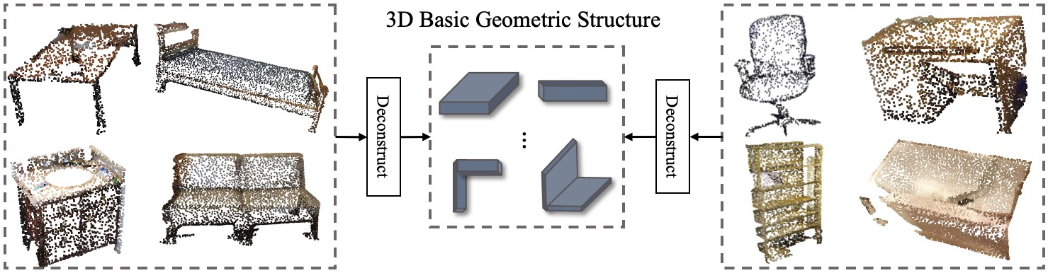
Figure 1: Illustration of the basic geometry of 3D objects, which can be shared among classes.

Prototypical VoteNet incorporates two new modules, namely Prototypical Vote Module (PVM) and Prototypical Head Module (PHM), to enhance local and global feature learning, respectively, for few-shot 3D detection. Specifically, based on extracted features from a backbone network (i.e. PointNet++ [26]), PVM firstly constructs a class-agnostic 3D primitive memory bank to store geometric prototypes, which are shared by all categories and updated iteratively during training. To exploit the transferability of geometric structures, PVM then incorporates a multi-head cross-attention module to associate geometric prototypes with points in a given scene and utilize them to refine their feature representations. PVM is majorly developed to exploit shared geometric structures among base and novel categories to enhance feature learning of local information in the few-shot setting. Further, to facilitate learning discriminative features for object categorization, PHM is designed to employ a multi-head cross-attention module and leverage class-specific prototypes from a few support samples to refine global representations of objects. Moreover, episodic training [33, 39] is adopted to simulate few-shot circumstances, where PHM is trained by a distribution of similar few-shot tasks instead of only one target object detection task.

Our contributions are listed as follows:

• We are the first to study the promising few-shot 3D point cloud object detection task, which allows a model to detect new classes, given a few examples.

• We propose Prototypical VoteNet, which incorporates Prototypical Vote Module and Prototypical Head Module, to address this new challenge. Prototypical Vote Module leverages class-agnostic geometric prototypes to enhance the local features of novel samples. Prototypical Head Module utilizes the class-specific prototypes to refine the object features with the aid of episode training.

• We contribute two new benchmark dataset settings called FS-ScanNet and FS-SUNRGBD, which are specifically designed for this problem. Our experimental results on these two benchmark datasets show that the proposed model effectively addresses the few-shot 3D point cloud object detection problem, yielding significant improvement over several competitive baseline approaches.

2 Related Work

3D Point Cloud Object Detection. Current 3D point cloud object detection approaches can be divided into two streams: Grid Projection/Voxelization based [48, 16, 36, 4, 54, 42] and point-based [31, 23, 19, 9, 2]. The former projects point cloud to 2D grids or 3D voxels so that the advanced convolutional networks can be directly applied. The latter methods take the raw point cloud feature extraction network such as PointNet++ [26] to generate point-wise features for the subsequent detection. Although these fully supervised approaches achieved promising 3D detection performance, their requirement for large amounts of training data precludes their application in many real-world scenarios where training data is costly or hard to acquire. To alleviate this limitation, we explore the direction of few-shot 3D object detection in this paper.

Few-Shot Recognition. Few-shot recognition aims to classify novel instances with abundant base samples and a few novel samples. Simple pre-training and finetuning approaches first train the model on the base classes, then finetune the model on the novel categories [3, 8]. Meta-learning based methods [10, 17, 12, 39, 33] are proposed to learn classifier across tasks and then transfer to the few-shot classification task. The most related work is Prototypical Network [33], which represents a class as one prototype so that classification can be performed by computing distances to the prototype representation of each class. The above works mainly focus on 2D image understanding. Recently, some few-shot learning approaches for point cloud understanding [30, 53, 49] are proposed. For instance, Sharma et al. [53] propose a graph-based method to propagate the knowledge from few-shot samples to the input point cloud. However, there is no work studying few-shot 3D point cloud object detection. In this paper, we first study this problem and introduce the spirit of Prototypical Network into few-shot 3D object detection with 3D geometric prototypes and 3D class-specific prototypes.

2D Few-shot Object Detection. Most existing 2D few-shot detectors employ a meta-learning [41, 15, 47] or fine-tuning based mechanism [45, 44, 27, 37]. Particularly, Kang et al. [15] propose a one-stage few-shot detector which contains a meta feature learner and a feature re-weighting module. Meta R-CNN [47] presents meta-learning over RoI (Region-of-Interest) features and incorporates it into Faster R-CNN [29] and Mask R-CNN [12]. TFA [40] reveals that simply fine-tuning the box classifier and regressor outperforms many meta-learning based methods. Cao et al. [1] improve the few-shot detection performance by associating each novel class with a well-trained base class based on their semantic similarity.

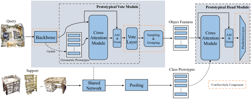
Figure 2: Illustration of Prototypical VoteNet. Prototypical VoteNet introduces two modules for few-shot 3D detection: 1) Prototypical Vote Module for enhancing local feature representation of novel samples by leveraging the geometric prototypes, 2) Prototypical Head Module for refining global features of novel objects, utilizing the class-specific prototypes.

3 Our Approach

In few-shot 3D point cloud object detection (FS3D), the object class set $\mathbb{C}$ is split into $\mathbb{C}_{\text{base}}$ and $\mathbb{C}_{\text{novel}}$ such that $\mathbb{C}=\mathbb{C}_{\text{base}}\cup\mathbb{C}_{\text{novel}}$ and $\mathbb{C}_{\text{base}}\cap\mathbb{C}_{\text{novel}}=\emptyset$. For each class $r\in\mathbb{C}$, its annotation dataset $T_{r}$ contains all the data samples with object bounding boxes, that is $T_{r}=\{(u,P)|u\in\mathbb{R}^{6},P\in\mathbb{R}^{N\times 3}\}$. Here, $(u,P)$ is a 3D object bounding box $u=(x,y,z,h,w,l)$, representing box center locations and box dimensions, in a point cloud scene $P$.

There are only a few examples/shots for each novel class $r\in\mathbb{C}_{\text{novel}}$, which are known as support samples. Besides, there are plenty of annotated samples for each base class $r\in\mathbb{C}_{\text{base}}$. Given the above dataset, FS3D aims to train a model to detect object instances in the novel classes leveraging such sufficient annotations for base categories $\mathbb{C}_{\text{base}}$ and limited annotations for novel categories $\mathbb{C}_{\text{novel}}$.

In the following, we introduce Prototypical VoteNet for few-shot 3D object detection. We will describe the preliminaries of our framework in Section 3.1, which adopts the architecture of VoteNet-style 3D detectors [25, 52, 2]. Then, we present Prototypical VoteNet consisting of Prototypical Vote Module (Section 3.2.1) and Prototypical Head Module (Section 3.2.2) to enhance feature learning for FS3D.

3.1 Preliminaries

VoteNet-style 3D detectors [25, 52, 2] takes a point cloud scene $P_{i}$ as input, and localizes and categorizes 3D objects. As shown in Figure 2, it firstly incorporates a 3D backbone network (i.e. PointNet++ [26]) parameterized by $\theta_{1}$ with downsampling layers for point feature extraction as Equation (1).

$$F_{i}=h_{1}(P_{i};\theta_{1}),$$ (1)

where $N$ and $M$ represent the original and subsampled number of points, respectively, $P_{i}\in\mathbb{R}^{N\times 3}$ represents an input point cloud scene $i$, and $F_{i}\in\mathbb{R}^{M\times(3+d)}$ is the subsampled scene points (also called seeds) with $d$-dimensional features and $3$-dimensional location coordinates.

Then, $F_{i}$ is fed into the vote module with parameters $\theta_{2}$ which outputs a $3$-dimensional coordinate offset $\Delta d_{j}=(\Delta x_{j},\Delta y_{j},\Delta z_{j})$ relative to its corresponding object center $c=(c_{x},c_{y},c_{z})$ and a residual feature vector $\Delta f_{j}$ for each point $j$ in $F_{i}=\{f_{j}\}_{i}$ as in Equation (2).

$$\{\Delta d_{j},\Delta f_{j}\}_{i}=h_{2}(F_{i};\theta_{2}).$$ (2)

Given the predicted offset $\Delta d_{j}$, the estimated corresponding object center $c_{j}=(c_{x_{j}},c_{y_{j}},c_{z_{j}})$ that point $j$ belongs to can be calculated as Equation (3).

$$c_{x_{j}}=x_{j}+\Delta x_{j},c_{y_{j}}=y_{j}+\Delta y_{j},c_{z_{j}}=z_{j}+\Delta z_{j}.$$ (3)

Similarly, the point features are updated as $F_{i}\leftarrow F_{i}+\Delta F_{i}$ where $\Delta F_{i}=\{\Delta f_{j}\}_{i}$.

Next, the detector samples object centers from $\{(c_{x_{j}},c_{y_{j}},c_{z_{j}})\}_{i}$ using farthest point sampling and group points with nearby centers together (see Figure 2: Sampling $\&$ grouping) to form a set of object proposals $O_{i}=\{o_{t}\}_{i}$. Each object proposal is characterized by a feature vector $f_{o_{t}}$ which is obtained by applying a max pooling operation on features of all points belonging to $o_{t}$.

Further, equipped with object features $\{f_{o_{t}}\}_{i}$, the prediction layer with parameters $\theta_{3}$ is adopted to yield the bounding boxes $b_{t}$, objectiveness scores $s_{t}$, and classification logits $r_{t}$ for each object proposal $o_{t}$ following Equation (4).

$$\{b_{t},s_{t},r_{t}\}_{i}=h_{3}(\{f_{o_{t}}\}_{i};\theta_{3}).$$ (4)

3.2 Prototypical VoteNet

Here, we present Prototypical VoteNet which incorporates two new designs – Prototypical Vote Module (PVM) and Prototypical Head Module (PHM) to improve feature learning for novel categories with few annotated samples (see Figure 2). Specifically, PVM builds a class-agnostic memory bank of geometric prototypes $\mathcal{G}=\{g_{k}\}_{k=1}^{K}$ with a size of $K$, which models transferable class-agnostic 3D primitives learned from rich base categories, and further employs them to enhance local feature representation for novel categories via a multi-head cross-attention module. The enhanced features are then utilized by the Vote Layer to output the offset of coordinates and features as Equation (2). Second, to facilitate learning discriminative features for novel class prediction, PHM employs an attention-based design to leverage class-specific prototypes $\mathcal{E}=\{e_{r}\}_{r=1}^{R}$ extracted from the support set $D_{\text{support}}$ with $R$ categories to refine global discriminate feature for representing each object proposal (see Figure 2). The output features are fed to the prediction layer for producing results as Equation (4). To make the model more generalizable to novel classes, we exploit the episodic training [33, 39] strategy to train PHM, where a distribution of similar few-shot tasks instead of only one object detection task is learned in the training phase. PVM and PHM are elaborated in the following sections.

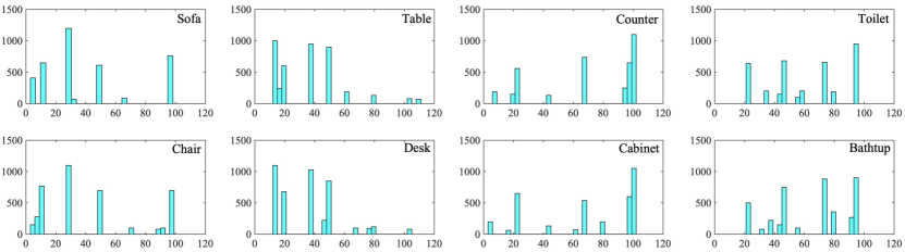
Figure 3: Visualization of the assignment of object point features to the geometric prototypes, where the horizontal axis represents the index of geometric prototypes and the vertical axis represents the number of assignments.

3.2.1 Prototypical Vote Module

Given input features $F_{i}$ extracted by a backbone network, Prototypical Vote Module constructs class-agnostic geometric prototypes $\mathcal{G}=\{g_{k}\}_{k=1}^{K}$ and then uses them to enhance local point features with an attention module.

Geometric Prototype Construction.

At the beginning, $\mathcal{G}=\{g_{k}\}_{k=1}^{K}\in\mathbb{R}^{d\times K}$ is randomly initialized. During training, $\mathcal{G}$ is iteratively updated with a momentum based on point features of foreground objects. Specifically, for each update, given $\mathcal{G}=\{g_{k}\}_{k=1}^{K}$ and all the foreground points $\{p_{m}\}_{m=1}^{M_{f}}$ with features $\{f_{m}\}_{m=1}^{M_{f}}$, where $M_{f}$ is the number of foreground points in the current batch, we assign each point to its nearest geometric prototype based on feature space distance. Then, for each prototype $g_{k}$, we have a group of points $\{p_{m}\}_{k}$ with features represented as $\{f_{m}\}_{k}$ assigned to it. Point features in one group are averaged to update the corresponding geometric prototype as Equation (5).

$$g_{k}\leftarrow\gamma*g_{k}+(1-\gamma)\overline{f}_{k},\text{where}~{}\overline{f}_{k}=\text{average}(\{f_{m}\}_{k}).$$ (5)

Here $\gamma\in[0,1]$ is the momentum coefficient for updating geometric prototypes in a momentum manner, serving as a moving average over all training samples. Since one point feature is related to one geometric prototype, we call this one-hot assignment strategy as hard assignment. An alternative to the hard assignment is the soft assignment, which calculates the similarity between a point features with all geometric prototypes. Empirically, we found that hard assignment results in more effective grouping versus soft assignment. More details can be found in the supplementary material.

Geometric Prototypical Guided Local Feature Enrichment.

Given the geometric prototypes $\mathcal{G}=\{g_{k}\}_{k=1}^{K}$ and point features $F_{i}=\{f_{j}\}_{i}$ of a scene $i$, PVM further employs a multi-head cross-attention module [38] to refine the point features. Specifically, the multi-head attention network uses the point features $F_{i}=\{f_{j}\}_{i}$ as query, geometric prototypes $\mathcal{G}=\{g_{k}\}_{k=1}^{K}$ as key and value where linear transformation functions with weights represented as $Q_{h},U_{h},V_{h}$ are applied to encode query, key and value respectively. Here, $h$ represents the head index. Then, for each head $h$, the query point feature is updated by softly aggregating the value features where the soft aggregation weight is determined by the similarity between the query point feature and corresponding key feature. The final point feature $f_{j}$ is updated by summing over outputs from all heads as Equation (6).

$$f_{j}\leftarrow\text{Cross\_Att}(f_{j},\{g_{k}\})=\sum_{h=1}^{H}W_{h}(\sum_{k=1}^{K}A^{h}_{j,k}\cdot V_{h}g_{k}),\text{where}~{}A^{h}_{j,k}=\frac{\exp[(Q_{h}f_{j})^{T}(U_{h}g_{k})]}{\sum_{k=1}^{K}{\exp[(Q_{h}f_{j})^{T}(U_{h}g_{k})]}}.$$ (6)

Here, $A_{j,k}^{h}$ is the soft aggregation weight considering the similarity between the $j$-th query point feature and the $k$-th key feature and used to weight the $k$-th value feature. Through this process, the point feature is refined using geometric prototypes in a weighted manner where prototypes similar to the query point feature will have higher attention weights. This mechanism transfers geometric prototypes learned from base categories with abundant data to model novel points. The multi-head design enables the model to seek similarity measurements from different angles in a learnable manner to improve robustness. Additionally, in both PHM and PVM, the multi-head attention layer are combined with feed forward FC layers. After refining point features $\{f_{j}\}_{i}$, PVM predicts the point offset and residual feature vector $\{\Delta d_{j},\Delta F_{j}\}_{i}$ as stated in Equation  (2). $\Delta d_{j}$ is explicitly supervised by a regression loss $\mathcal{L}_{\text{vote}}$ used in [26].

What do the geometric prototypes store?

To shed more insights on what the geometric prototypes represent, we visualize the frequency of geometry prototypes in different categories using the “assignment”. The number of “assignment”s of object point features to the geometric prototypes is shown in Figure 3, where a point is assigned to the geometric prototype with the highest similarity. In each histogram, the horizontal axis represents the index of geometric prototypes and the vertical axis represents the number of assignments. Note that the first row is the novel classes and the second row is the base classes. Figure 3 shows that two visually similar categories have a similar assignment histogram since they share the basic geometric structures. This indicates that the memory bank of geometric prototypes successfully learns the 3D basic geometric knowledge, which can be a bridge to transfer the geometric knowledge from base classes to novel ones.

3.2.2 Prototypical Head Module

As shown in Figure 2, given object proposals $O_{i}=\{o_{t}\}_{i}$ with features $\{f_{o_{t}}\}_{i}$ from Sampling & Grouping module, PHM module leverages class-specific prototypes $\{e_{r}\}$ to refine the object features $f_{o_{t}}$ for the subsequent object classification and localization. Moreover, for better generalizing to novel categories, PHM is trained by the episodic training scheme, where PHM learns a large number of similar few-shot tasks instead of only one task. Considering the function of PHM, we construct the few-shot tasks that, in each iteration, PHM refines the object features $\{f_{o_{t}}\}_{i}$ with the aid of class-specific prototypes, which are extracted from randomly sampled support samples.

In each few-shot task, class-specific prototypes are built based on support sets that are randomly sampled. For class $r$, the class-specific prototype $e_{r}$ is obtained by averaging the instance features for all support samples in class $r$. The instance feature is derived by applying a max pooling operation over the features of all points belonging to that instance. As shown in Figure 2, with class-specific prototypes $\mathcal{E}=\{e_{r}\}_{r=1}^{R}$ for a total of $R$ categories, PHM further employs a multi-head cross-attention module to refine object features $\{f_{o_{t}}\}_{i}$. Here, the object features $\{f_{o_{t}}\}_{i}$ serve as the query features, class-specific prototypes are used to build value features and key features similar as what has been described in Section 3.2.1. Then, the representation $f_{o_{t}}$ of each proposal $o_{t}$ is refined using the outputs of the multi-head attention module, which are weighted sum over the value features and the weight is proportionally to the similarity between the query feature and corresponding key features. This process can be formulated as Equation (7), which is similar to Equation (6).

$$f_{o_{t}}\leftarrow\text{Cross\_Att}(f_{o_{t}},\{e_{r}\}).$$ (7)

Until now, $f_{o_{t}}$ is refined using class-specific prototypes, injecting class-specific features from given support samples into object-level features. Finally, the refined object features $\{f_{o_{t}}\}_{i}$ are fed into the prediction module following Equation (4).

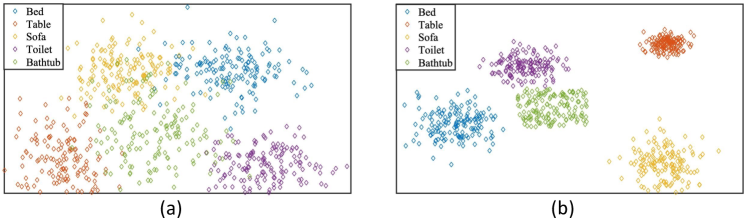
Figure 4: t-SNE visualization of the effect of PHM. (a) shows the features without being processed by PHM. (b) shows the features processed by PHM using class-specific prototypes.

What does PHM help?

Figure 4 visualizes the effect of feature refinement by PHM. The experiment is conducted on FS-ScanNet. Figure 4(a) shows the object features, which have not been processed by PHM. Figure 4(b) shows the object features processed by PHM. We could observe that, after the feature refinement by PHM, the features of each classes become more compact compared to the non-PHM one, which further validates the effectiveness of PHM.

3.3 Model Training

The model is trained by the episodic training strategy [33, 39]. The detailed training strategy is included in the supplementary material. We use the standard cross entropy loss $\mathcal{L}_{\text{cls}}$ and smooth-$L_{1}$ loss [29] $\mathcal{L}_{\text{reg}}$ to supervise the classification and the bounding box regression, respectively. As for the objectness prediction, if a vote is located either within 0.3 meters to a ground truth object center or more than 0.6 meters from any center, it is considered to be positive [25], which is supervised by a cross entropy loss $\mathcal{L}_{\text{obj}}$. Therefore, the overall loss for Prototypical VoteNet is given by,

$$\mathcal{L}_{\text{det}}=\mathcal{L}_{\text{cls}}+\alpha_{1}\mathcal{L}_{\text{reg}}+\alpha_{2}\mathcal{L}_{\text{obj}}+\alpha_{3}\mathcal{L}_{\text{vote}},$$ (8)

where $\alpha_{1},\alpha_{2},\alpha_{3}$ is the coefficients to balance the loss contributions.

4 Experiments

To our best knowledge, there is no prior study of few-shot point cloud object detection. Therefore, we setup a new benchmark which is described in Section 4.1 &  4.2. Then, we conduct experiments and compare our method with baseline methods in Section 4.3. Third, a series of ablation studies are performed for further analyzing Prototypical VoteNet in Section 4.4. In addition, the implementation details are included in the supplementary material.

4.1 Benchmark Setup

Datasets.

We construct two new benchmark datasets FS-SUNRGBD and FS-ScanNet. Specifically, FS-SUNRGBD is derived from SUNRGBD [35]. SUNRGBD consists of  5K RGB-D training images annotated, and the standard evaluation protocol reports performance on 10 categories. We randomly select 4 classes as the novel ones while keeping the remaining ones as the base. In the training set, only $K$ annotated bounding boxes for each novel class are given, where k equals 1, 2, 3, 4 and 5. FS-ScanNet is derived from ScanNet [6]. ScanNet consists of 1,513 point clouds, and the annotation of the point clouds corresponds to 18 semantic classes plus one for the unannotated space. Out of its 18 object categories, we randomly select 6 classes as the novel ones, while keeping the remaining as the base. We evaluate with 2 different base/novel splits. In the training set, only $K$ annotated bounding boxes for each novel class are given, where k equals 1, 3 and 5. More details about the new benchmark datasets can be referred to the supplementary material.

Evaluation Metrics. We follow the standard evaluation protocol [25] in 3D point cloud object detection by using mean Average Precision(mAP) under different IoU thresholds (i.e. 0.25, 0.50), denoted as AP₂₅ and AP₅₀. In addition, in the inference stage, we detect both novel classes and base classes. The performance on base classes is included in the supplementary material.

4.2 Benchmark Few-shot 3D Object Detection

We build the first benchmark for few-shot 3D object detection. The benchmark incorporates 4 competitive methods, and three of them are built with few-shot learning strategies, which have been shown to be successful in 2D few-shot object detection.

• Baseline: We abandon PVM and PHM, and train the detector on the base and novel classes together. In this way, it can learn good features from the base classes that are applicable for detecting novel classes.

• VoteNet+TFA [40]: We incorporate a well-designed few-shot object detection method TFA [40] with VoteNet. TFA first trains VoteNet on the training set with abundant samples of base classes. Then only the classifier and the regressor are finetuned with a small balance set containing both base classes and novel classes.

• VoteNet+PT+TFA: The pretraining is proven to be important in 2D few-shot learning, as it learns more generic features, facilitating knowledge transfer from base classes to novel classes. Therefore, we add a pretraining stage, which is borrowed from a self-supervised point cloud contrastive learning method [14], before the training stage of VoteNet+TFA.

• Meta VoteNet: Meta VoteNet is inspired by Meta RCNN [47]. Meta RCNN develops a meta-learning prediction head, which leverages class prototypes to multiply the RoI features and then predicts if a RoI feature is the category that the class prototype belongs to. In VoteNet, the grouped point features after the vote stage can be treated as the RoI features.

4.3 Main Results

FS-ScanNet.

We first compare the proposed approach with the baselines on FS-ScanNet in Table 1. These results show: 1) VoteNet+TFA has the worst performance. For example, it only achieves 8.07% AP₂₅ and 1.03% AP₅₀ on 3-shot in Novel Split-1. The reason is that VoteNet+TFA is trained from scratch, and only a few layers are funetuned by novel samples. Therefore, it tends to be overfitting with poor generalization ability on novel classes. 2) Even adding a pretaining stage to VoteNet+TFA, which is termed as VoteNet+PT+TFA, it still performs poorly. For example, it only contributes the improvement of +2.30% AP₂₅ and +1.10% AP₅₀ to VoteNet+TFA on 3-shot in Novel Split-1. This is different from 2D few-shot object detection. This is potentially caused by the lack of large-scale datasets for pre-training in 3D, while the 2D backbone ResNet [13] has a dataset of over one million images for pre-training. 3) Besides our designed method, Meta VoteNet is superior. For example, Meta VoteNet reaches 25.73% AP₂₅ and 16.01% AP₅₀ on 3-shot in Novel Split-1. This shows the meta-learning prediction head, derived from Meta RCNN [47], helps to generalize from base classes to novel classes. 4) Our new model Prototypical VoteNet surpasses all competitors by significant margins. For example, Prototypical VoteNet achieves 32.25% AP₂₅ and 16.01% AP₅₀ on 3-shot in Novel Split-1. This is because our proposed method is equipped with a more generic vote module by learning geometric prototypes, and leverage class prototypes to promote the discriminative feature learning.

Method	Novel Split 1						Novel Split 2
	1-shot		3-shot		5-shot		1-shot		3-shot		5-shot
	AP25	AP50	AP25	AP50	AP25	AP50	AP25	AP50	AP25	AP50	AP25	AP50
Baseline	9.21	3.14	22.64	9.04	24.93	12.82	4.92	0.94	15.86	3.15	20.72	6.13
VoteNet+TFA	0.48	0.09	8.07	1.03	16.36	7.91	1.00	0.15	2.64	0.22	5.71	2.40
VoteNet+PT+TFA	2.58	1.04	10.37	2.13	17.21	8.94	2.13	0.56	4.85	1.25	7.25	2.49
Meta VoteNet	11.01	4.20	25.73	10.99	26.68	14.40	6.06	1.01	16.93	4.51	23.83	7.17
Ours	15.34	8.25	31.25	16.01	32.25	19.52	11.01	2.21	21.14	8.39	28.52	12.35

Table 1: Results on FS-ScanNet using mean Average Precision (mAP) at two different IoU thresholds of 0.25 and 0.50, denoted as AP₂₅ and AP₅₀.

Method	1-shot		2-shot		3-shot		4-shot		5-shot
	AP25	AP50	AP25	AP50	AP25	AP50	AP25	AP50	AP25	AP50
Baseline	5.46	0.22	6.52	0.77	13.73	2.20	20.47	4.50	22.99	5.90
VoteNet+TFA	1.41	0.03	3.70	0.78	4.03	1.09	7.91	2.10	8.50	2.81
VoteNet+PT+TFA	3.40	0.51	5.13	1.22	7.94	2.31	10.05	3.12	11.32	4.01
Meta VoteNet	7.04	0.98	9.23	1.34	16.24	3.12	20.10	4.69	24.41	6.05
Ours	12.39	1.52	14.54	3.05	21.51	6.13	24.78	7.17	29.95	8.16

Table 2: Results on FS-SUNRGBD using mean Average Precision (mAP) at two different IoU thresholds of 0.25 and 0.50, denoted as AP₂₅ and AP₅₀.

FS-SUNRGBD.

Table 2 shows the result comparison on FS-SUNRGBD. In FS-SUNRGBD, we find that VoteNet+TFA and VoteNet+PT+TFA still have a large gap with other methods due to the overfitting and insufficient pretraining. Meanwhile, Meta VoteNet outperforms other baseline methods. For example, on 3-shot, Meta VoteNet surpasses VoteNet+PT+TFA by +8.34% AP₂₅ and +0.81% AP₅₀ and achieves 16.24% AP₂₅ and 3.12% AP₅₀. Finally, our designed Prototypical VoteNet outperforms all the methods. For instance, on 3-shot, Prototypical VoteNet surpasses Meta VoteNet by +5.37% AP₂₅ and +3.01% AP₅₀, which further validates the effectiveness of our proposed PVM and PHM.

4.4 Further Analysis

Method	3-shot		5-shot
	AP25	AP50	AP25	AP50
Baseline	22.64	9.04	24.93	12.82
+PVM	27.43	13.63	28.44	16.45
+PHM	28.76	14.04	30.13	17.51
+PVM+PHM	31.25	16.01	32.25	19.52

Table 3: Ablation study of individual components.

	Prototype	AP0.25	AP0.50
PVM	Geometric	31.25	16.01
	Self-learning	28.34	14.01
PHM	Class	31.25	16.01
	Self-learning	27.45	13.67

Table 4: Ablation study of Prototypes.

Contributions of individual components.

We conduct ablation studies on 3-shot and 5-shot in split-1 of FS-ScanNet with results shown in Table 4.4. The results show that both of them are effective on their own. For example, on 3-shot, PVM contributes the improvement of +4.19% AP₂₅ and +4.59% AP₅₀, and PHM contributes the improvement of +6.12% AP₂₅ and +5.00% AP₅₀. Moreover, when combined, the best performance, 31.25% AP₂₅ and 16.01% AP₅₀, is achieved.

Effectiveness of Prototypes.

Table  4.4 shows the effectiveness of two kinds of prototypes. In order to validate the geometric prototypes, we displace them by the self-learning ones, which are randomly initialized and updated by the gradient descend during the model training. Table  4.4 results show that the performance significantly degrades. To validate the effectiveness of class prototypes, we also alter them by the randomly initialized self-learning prototypes. Similarly, the performance drops drastically due to the lack of class prototypes.

# Prototype	AP0.25	AP0.50
$K=30$	29.98	15.01
$K=60$	30.24	15.54
$K=90$	31.10	15.98
$K=120$	31.25	16.01
$K=150$	31.01	15.89

Table 5: Ablation study of memory bank size.

Coefficient $m$	AP0.25	AP0.50
$\gamma=0.2$	29.50	14.65
$\gamma=0.9$	30.55	15.15
$\gamma=0.99$	30.71	15.30
$\gamma=0.999$	31.01	15.89
$\gamma=0.9999$	30.90	15.79

Table 6: Ablation study of coefficient $\gamma$.

Size of Memory Bank.

Table 4.4 studies the size of the memory bank containing the geometric prototypes. This ablation study is performed on 3-shot in split-1 of FS-ScanNet. The value of K is set to $\{30,60,90,120,150\}$. For $\text{K}=30$, the memory bank only contains 30 geometric prototypes, which only achieves 29.98% AP₂₅ and 15.01% AP₅₀. Furthermore, when using more prototypes (i.e., $\text{K}=120$), there will be an obvious performance improvement, which reaches 31.25% AP₂₅ and 16.01% AP₅₀. However, when continuous increasing K, there will be no improvement. Therefore, we set the size of the memory bank to be 120.

Coefficient $\gamma$.

Table 4.4 shows the effect of momentum coefficient ($\gamma$ in Equation (5)). The experiment is performed on 3-shot in split 1 of FS-ScanNet. The results show that, when using a relatively large coefficient (i.e., $\gamma\in[0.999,0.9999]$), the model performs well, compared with the model using a small momentum coefficient (i.e., $\gamma\in[0.9,0.99]$). Moreover, the performance drops when using a small value of $\gamma=0.2$. The is potentially because a small momentum coefficient might bring about unstable prototype representation with rapid prototype updating.

Method	Novel Split 1						Novel Split 2
	1-shot		3-shot		5-shot		1-shot		3-shot		5-shot
	AP25	AP50	AP25	AP50	AP25	AP50	AP25	AP50	AP25	AP50	AP25	AP50
VoteNet+TFA	0.48	0.09	8.07	1.03	16.36	7.91	1.00	0.15	2.64	0.22	5.71	2.40
VoteNet+TFA∗	10.38	3.96	23.77	9.83	26.02	13.96	5.12	0.95	16.23	3.72	21.89	6.76
Ours	15.34	8.25	31.25	16.01	32.25	19.52	11.01	2.21	21.14	8.39	28.52	12.35

Table 7: Results of VoteNet+TFA^∗ on FS-ScanNet using mean Average Precision (mAP) at two different IoU thresholds of 0.25 and 0.50, denoted as AP₂₅ and AP₅₀.

Method	3-shot		5-shot
	AP25	AP50	AP25	AP50
GroupFree + DeFRCN	25.22	10.90	26.42	14.01
GroupFree + FADI	25.73	11.02	27.12	14.32
3DETR + DeFRCN	26.01	10.95	26.88	14.45
3DETR + FADI	26.24	11.12	26.93	15.22
Ours	31.25	16.01	32.25	19.52

Table 8: More Methods Borrowed From 2D Few-Shot Object detection

More Analysis on TFA.

TFA [40] is a simple yet effective method in few-shot 2D object detection. Specifically, TFA first trains a detector on the training set with abundant samples of base classes and then finetunes the classifier and the regressor on a small balanced set, which contains both base classes and novel classes. More details can be referred to in [40]. However, as shown in Table 1 and Table 2 in the main paper, VoteNet+TFA performs poorly in few-shot 3D object detection. As discussed in Section 4.3 in the main paper, the reason is that a few layers are finetuned by the samples of novel classes. A question arises here: why does TFA in few-shot 2D object detection only need to train the classifier and the regressor on the novel samples? We speculate that the large-scale pre-training on ImageNet [7] helps. To overcome this problem, in the first stage of TFA, we train the VoteNet on the training set with both novel classes and base classes. Then, in the second stage, we use a small balanced set containing both novel classes and base classes to finetune the classifier and the regressor. We denote this new baseline as VoteNet+TFA^∗. As shown in Table 7, VoteNet+TFA^∗ boosts the performance significantly. For example, in 3-shot in split-1 of FS-ScanNet, VoteNet+TFA^∗ can achieve 26.02% AP₂₅ and 13.96% AP₅₀, while VoteNet+TFA only reaches 16.36% AP₂₅ and 7.91% AP₅₀.

More Methods Borrowed From 2D Few-Shot Object detection.

We combine two SOTA 2D few-shot object detection techniques (i.e. DeFRCN [27], FADI [1]) and two SOTA 3D detectors (i.e. GroupFree [19], 3DETR [23]). These two few-shot techniques are plug-in-play modules and can be easily incorporated into the different detection architectures. We conducted this experiment on 3-shot and 5-shot in split-1 of FS-ScanNet. The results in Table 8 show that our method still surpasses these methods by a large margin. This is potentially because, in the 2D domain, they often build their model upon a large-scale pre-trained model on ImageNet. However, in the 3D community, there does not exist a large-scale dataset for model pre-training, which requires future investigations. Therefore, these 2D few-shot object detection techniques might not be directly transferable to the 3D domain. For future works, we might resort to the pre-training models in the 2D domain to facilitate the few-shot generalization on 3D few-shot learning and how these techniques can be combined with our method.

5 Concluding Remarks

In this paper, we have presented Prototypical VoteNet for FS3D along with a new benchmark for evaluation. Prototypical VoteNet enjoys the advantages of two new designs, namely Prototypical Vote Module (PVM) and Prototypical Head Module (PHM), for enhancing feature learning in the few-shot setting. Specifically, PVM exploits geometric prototypes learned from base categories to refine local features of novel categories. PHM is proposed to utilize class-specific prototypes to promote discriminativeness of object-level features. Extensive experiments on two new benchmark datasets demonstrate the superiority of our approach. We hope our studies on 3D propotypes and proposed new benchmark could inspire further investigations in few-shot 3D object detection.

Checklist

The checklist follows the references. Please read the checklist guidelines carefully for information on how to answer these questions. For each question, change the default [TODO] to [Yes] , [No] , or [N/A] . You are strongly encouraged to include a justification to your answer, either by referencing the appropriate section of your paper or providing a brief inline description. For example:

• Did you include the license to the code and datasets? [Yes] See Section LABEL:gen_inst.

• Did you include the license to the code and datasets? [No] The code and the data are proprietary.

• Did you include the license to the code and datasets? [N/A]

Please do not modify the questions and only use the provided macros for your answers. Note that the Checklist section does not count towards the page limit. In your paper, please delete this instructions block and only keep the Checklist section heading above along with the questions/answers below.

1. For all authors…

   1. Do the main claims made in the abstract and introduction accurately reflect the paper’s contributions and scope? [Yes]

   2. Did you describe the limitations of your work? [Yes] we have included limitation discussion in the supplementary material Section A.7.

   3. Did you discuss any potential negative societal impacts of your work? [N/A]

   4. Have you read the ethics review guidelines and ensured that your paper conforms to them? [Yes]

2. If you are including theoretical results…

   1. Did you state the full set of assumptions of all theoretical results? [N/A]

   2. Did you include complete proofs of all theoretical results? [N/A]

3. If you ran experiments…

   1. Did you include the code, data, and instructions needed to reproduce the main experimental results (either in the supplemental material or as a URL)? [Yes]

   2. Did you specify all the training details (e.g., data splits, hyperparameters, how they were chosen)? [Yes]

   3. Did you report error bars (e.g., with respect to the random seed after running experiments multiple times)? [Yes]

   4. Did you include the total amount of compute and the type of resources used (e.g., type of GPUs, internal cluster, or cloud provider)? [Yes]

4. If you are using existing assets (e.g., code, data, models) or curating/releasing new assets…

   1. If your work uses existing assets, did you cite the creators? [Yes]

   2. Did you mention the license of the assets? [Yes]

   3. Did you include any new assets either in the supplemental material or as a URL? [Yes]

   4. Did you discuss whether and how consent was obtained from people whose data you’re using/curating? [Yes]

   5. Did you discuss whether the data you are using/curating contains personally identifiable information or offensive content? [Yes]

5. If you used crowdsourcing or conducted research with human subjects…

   1. Did you include the full text of instructions given to participants and screenshots, if applicable? [N/A]

   2. Did you describe any potential participant risks, with links to Institutional Review Board (IRB) approvals, if applicable? [N/A]

   3. Did you include the estimated hourly wage paid to participants and the total amount spent on participant compensation? [N/A]

Appendix A Appendix

In this supplemental material, we will include the details of dataset split in Section A.1, the experimental results on base classes in Section A.2, the ablation study of hard and soft assignment in Section A.3, implementation and training details of Prototypical VoteNet in Section A.4, implementation details of the baseline method Meta VoteNet in Section A.5, visualization of basic geometric primitives in Section A.6, KNN baselines in Section A.7, non-updated prototypes in Section A.8, performance on the unbalance Problem in Section A.9 and limitation analysis in Section A.10.

A.1 Dataset Split

Table 9 lists the names of novel classes for FS-SUNRGBD and FS-ScanNet.

FS-SUNRGBD	FS-ScanNet(Split-1)	FS-ScanNet(Split-2)
table, bed, nightstand, toilet	sofa, window, bookshelf, toilet, bathtub, garbagebin	bed, table, door, counter, desk, showercurtain

Table 9: Names of novel classes for FS-SUNRGBD and FS-ScanNet.

A.2 Results on Base Classes

Method	FS-ScanNet				FS-SUNRGBD
	Split 1		Split 2
	AP25	AP50	AP25	AP50	AP25	AP50
VoteNet+TFA	51.00	24.22	51.50	30.73	36.57	10.61
VoteNet+PT+TFA	52.78	25.46	52.04	30.57	38.03	15.44
Meta VoteNet	52.13	25.13	47.89	28.44	40.22	20.60
VoteNet	57.96	32.60	54.63	35.76	47.77	26.78
Ours	53.83	28.20	51.22	32.41	46.07	25.26

Table 10: Results on FS-ScanNet and FS-SUNRGBD on base classes using mean Average Precision (mAP) at two different IoU thresholds of 0.25 and 0.50, denoted as AP₂₅ and AP₅₀.

Since we detect both base and novel classes during inference, we also report the performance on base classes in Table 10. For simplicity, we average the results of all k-shot (e.g. k=1,3,5) in each split. Table 10 shows VoteNet achieves the best performance on base classes, because it is specifically designed as a fully supervised method for base classes. Compared with VoteNet, the performance of VoteNet+TFA and VoteNet+PT+TFA on base classes degrades by -6.96% AP₂₅ and -8.38% AP₅₀, and -5.18% AP₂₅ and -7.14% AP₅₀, respectively, on split-1 of FS-ScanNet. Moreover, Prototypical VoteNet retains much more ability to recognize base classes, which achieves 53.83% AP₂₅ and 28.20% AP₅₀ on split-1 of FS-ScanNet, and 46.07% AP₂₅ and 25.26% AP₅₀ on FS-SUNRGBD. Compared with our method, we can observe a significant performance degradation in finetuning based methods. The reason is that, without the large-scale pre-training, a detector cannot learn more generic feature representation so as to transfer knowledge from base classes to novel classes. Under this circumstance, if we force the knowledge transferring by finetuning, it will distort the learned feature space for base classes.

A.3 Hard vs. Soft Assignment

Method	3-shot		5-shot
	AP25	AP50	AP25	AP50
Soft	27.24	12.82	29.13	15.13
Hard	31.25	16.01	32.25	19.52

Table 11: Ablation study of hard and soft assignment.

We leverage the hard assignment in Section 3.2.1: Geometric Prototype Construction, in the main paper. Here, we compare the original hard assignment in our implemented method with the soft assignment, which calculates the similarity between a point feature with all geometric prototypes and updates all geometric prototypes in a soft manner by the similarity scores between a point feature and the geometric prototypes. We conduct the experiment on 3-shot and 5-shot in split-1 of FS-ScanNet. The results in Table 11 indicate that the hard assignment is more effective than the soft assignment. This is because the geometric prototypes by the hard assignment are more distinctive than those using the soft assignment, since one geometric prototype is updated using the nearest point features without considering the others.

A.4 Implementation and Training Details

We follow recent practice [25, 46] to use PointNet++ [26] as a default backbone network. The backbone has 4 set abstraction layers and 2 feature propagation layers. For each set abstraction layer, the input point cloud is sub-sampled to 2048, 1024, 512, and 256 points with the increasing receptive radius of 0.2, 0.4, 0.8, and 1.2, respectively. Then, two feature propagation layers successively up-sample the points to 512 and 1024. Additionally, in both PHM and PVM, the multi-head attention layer are combined with feed forward FC layers. The details can be referred to our code. The size of memory bank of geometric prototypes is set to 120. The number of heads in both multi-head attention networks is empirically set to 4. The momentum coefficient is set to 0.999. We use 40k points in FS-ScanNet and 20k points in FS-SUNRGBD as input and adopt the same data augmentation as in  [25], including a random flip, a random rotation, and a random scaling of the point cloud by [0.9, 1.1].

Following the episodic training strategy [47], a training mini-batch in Prototypical VoteNet is comprised of a K-shot R-class support set $D_{\rm support}$ and a R-class query set $D_{\rm train}$ (the classes in $D_{\rm support}$ and $D_{\rm train}$ is consistent). Each sample in $D_{\rm support}$ is the whole point cloud scene. Before the pooling step, we use the groud-truth bounding boxes to obtain point features of target objects. The network is trained from scratch by the AdamW optimizer with 36 epochs. The weight decay is set to 0.01. The initial learning rate is 0.008 in FS-ScanNet and 0.001 in FS-SUNRGBD. Additionally, during the inference stage, we input both the query point cloud and the given support set to Prototypical VoteNet. Note that the features of the support point cloud only need to be extracted once, as they are independent of the query feature extraction.

A.5 Implementation Details of Meta VoteNet

We provide more details of the competitive baseline corresponding to Meta VoteNet in our main paper. It is derived from an effective few-shot 2D object detection approach - Meta RCNN [47]. In Meta RCNN, each RoI feature is fused with $R$ class prototypes using the channel-wise multiplication operator. As a result, a number of $R$ fused RoI features for each RoI are generated. Then each fused RoI feature is fed into the prediction layer for the binary prediction (whether the RoI feature is the category that the class prototype belongs to). More details can be referred to in [47]. We incorporate this meta-learning approach into VoteNet, namely Meta VoteNet. Similarly, after Sampling $\&$ Grouping (see Figure 2 in the main paper), we fuse point features of objects with $R$ class prototypes by the channel-wise multiplication operator. Then the binary class prediction and bounding box regression are conducted based on the fused features for classification and location prediction, respectively. For a fair comparison, Meta VoteNet shares the same architecture with Prototypical VoteNet, except Prototypical Vote Module and Prototypical Prediction Module. The training details follow the proposed Prototypical VoteNet.

A.6 Visualization of Basic Geometric Primitives

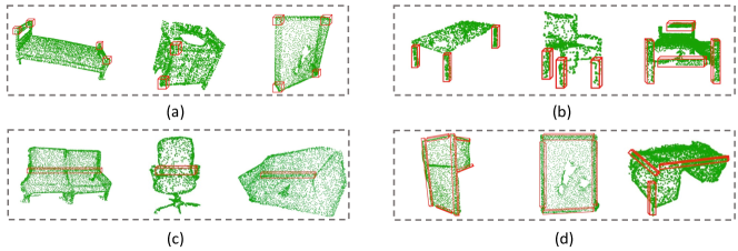
Figure 5: Visualization of some basic geometric primitives learned by the prototypes. (a) Corner, (b) Stick, (c) Hinge, (d) Edge.

In Figure 5, we visualize the relation between the learned geometric prototypes and the 3D points by searching points with features that are similar to a given geometric prototype. First, we feed object point clouds to a trained Prototypical VoteNet. Second, for each point feature, we can search for its most similar prototype. If the similarity is above a threshold, we can assign the point to that prototype. Third, we use a density-based clustering algorithm DBSCAN to cluster the point groups, and we draw the minimum 3D bounding box around each point group. As shown in the figure, all the red bounding boxes within each subfigure belong to the same prototype. The result shows that in each subfigure, the enclosed geometric structures are similar. For example, subfigure (a) illustrates that the prototype learns the feature of corners, while subfigure (b) shows that the prototype learns the long stick.

A.7 KNN Baselines

Method	3-shot		5-shot
	AP25	AP50	AP25	AP50
VoteNet + KNN	23.07	9.56	25.58	13.51
Group-Free + KNN	24.22	9.97	26.33	13.92
3DETR[2] + KNN	24.08	10.21	26.01	14.36
Ours	31.25	16.01	32.25	19.52

Table 12: KNN baselines.

We apply KNN assignment to VoteNet and two SOTA 3D detectors GroupFree [19] and 3DETR [23]. We conducted this experiment on 3-shot and 5-shot in split-1 of FS-ScanNet. The KNN assignment is realized by calculating the distance between each object feature and features of all training objects in the classification step, and assigning the sample to the class based on voting from its k-nearest objects of the training set. Here, we take k as one since we find increasing the value k doesn’t improve performance. The results are shown in Table 12. Comparing the performance of “VoteNet + KNN” and “ours”, we see that the non-parametric KNN classifier will not help improve few-shot learning much (“VoteNet” vs “VoteNet+KNN”). Comparing the performance of different detectors (“VoetNet+KNN”, “GroupFree + KNN”, and “3DETR+KNN”), we observe that a better detection architecture does not bring large performance gains in the few-shot 3D detection scenario. The most challenging issue for few-shot 3D object detection still lies in how to learn effective representation if only a few training samples are provided. The classifier and architecture don’t help much if the model cannot effectively extract features to represent novel categories with only a few samples.

A.8 Non-Updated Prototypes

Method	3-shot		5-shot
	AP25	AP50	AP25	AP50
Update	28.05	13.89	28.51	14.51
Non-Update	31.25	16.01	32.25	19.52

Table 13: Does setting the prototype at the end (no updates) perform well ?

As shown in Table 13, for the proposed Prototypical VoteNet, if we don’t update the prototype in PVM, the performance would degrade significantly. Without updating, the randomly initialized prototypes can not learn the geometry information from base classes in the training phase. In this case, it is hard to transfer the basic geometry information from base classes to the novel classes as the prototypes are meaningless.

A.9 Performance on the Unbalance Problem

Method	P		10P		25P		50P
	AP25	AP50	AP25	AP50	AP25	AP50	AP25	AP50
VoteNet	62.34	40.82	52.06	35.64	43.12	27.13	40.01	26.77
Ours	62.59	41.25	52.60	36.87	44.53	29.17	41.99	29.01

Table 14: Performance on the Unbalance Problem in ScanNet V2

Method	P		10P		25P		50P
	AP25	AP50	AP25	AP50	AP25	AP50	AP25	AP50
VoteNet	59.78	35.77	51.09	31.81	43.68	29.08	40.46	22.23
Ours	60.34	36.80	51.85	32.98	44.66	31.93	41.84	25.04

Table 15: Performance on the Unbalance Problem in SUN RGB-D

To analyze the performance of the proposed model on the imbalance problem, we conduct experiments using all the classes. Note that we conduct the experiments not only on ScanNet V2, but also on the more unbalanced counterparts. We follow the benchmark [5], to create these counterparts: 1) sorting the classes in descending order according to number of samples in each class, then we have $n_{i}>n_{j}$ if $i<j$, where $n$ is the number of samples, $i$ and $j$ denote the index of the classes. 2) reducing the number of training samples per class according to an exponential function $n=n_{i}*u^{i}$, where $u\in(0,1)$. The test set remains unchanged. According to the benchmark [5], we define the imbalance factor of a dataset as the number of training samples in the largest class divided by the smallest. Note that we use P as the value of the imbalance factor in ScanNet V2. Additionally, we add another three sets, whose values of imbalance factor are 10P, 25P and 50P for both ScanNet V2. As shown in Table 14, we achieve comparable performance in the original dataset setting. With the imbalance becoming more severe (e.g., 25P, 50P), our approach outperforms the baseline more. Note that our focus is on few-shot 3D object detection, where representation learning of new categories becomes the top consideration of algorithm design. This few-shot problem is more useful for scenarios where many new categories appear frequently and require the system to quickly adapt to recognize them. However, the long-tailed problem focuses on how to learn good representations and classifiers that can deliver good performance for both head and tail categories. We believe that dedicated designs can further improve the performance of long-tailed 3D object detection. We will also add the results and analysis for the long-tailed setting in our paper and hope to inspire more future investigations.

A.10 Limitation Analysis

Although the 3D cues of point clouds are more stable since they can get rid of some visual distractors, such as lighting and perspectives, some factors still impede the model from better generalization. For instance, in 3D scene understanding, if the point cloud in the training set is dense and that of the test set is sparse, a model often performs poorly, which can be treated as a cross-domain problem. Regarding few-shot 3D object detection, the performance might degrade if there is such a large domain gap between base classes and novel classes. Even though the basic geometric features are learned in the base classes, they might not be generalized well to the novel classes due to the difference in point cloud sparsity. The performance of this model has much room for improvement. One way to achieve better performance is large-scale pre-training. Large-scale pre-training enables the model to learn more generic features for transfer learning using limited samples, which benefits the community of 2D few-shot learning (i.e., ImageNet Pre-training). For future works, we might resort to the pre-training models in the 2D domain to facilitate the few-shot generalization on 3D few-shot learning and how these techniques can be combined with our method.

References

- [1] Cao, Y., Wang, J., Jin, Y., Wu, T., Chen, K., Liu, Z., Lin, D.: Few-shot object detection via association and discrimination. In: Advances in Neural Information Processing Systems (2021)
- [2] Chen, J., Lei, B., Song, Q., Ying, H., Chen, D.Z., Wu, J.: A hierarchical graph network for 3d object detection on point clouds. In: IEEE Conference on Computer Vision and Pattern Recognition (2020)
- [3] Chen, W.Y., Liu, Y.C., Kira, Z., Wang, Y.C.F., Jia-Bin, H.: A closer look at few-shot classification. In: International Conference on Learning Representations (2019)
- [4] Chen, X., Ma, H., Wan, J., Li, B., Xia, T.: Multi-view 3d object detection network for autonomous driving. In: IEEE Conference on Computer Vision and Pattern Recognition (2017)
- [5] Cui, Y., Jia, M., Lin, T.Y., Song, Y., Belongie, S.: Class-balanced loss based on effective number of samples. In: IEEE Conference on Computer Vision and Pattern Recognition (2019)
- [6] Dai, A., Chang, A.X., Savva, M., Halber, M., Funkhouser, T., Nießner, M.: Scannet: Richly-annotated 3d reconstructions of indoor scenes. In: IEEE Conference on Computer Vision and Pattern Recognition (2017)
- [7] Deng, J., Wei, D., Richard, S., Li-Jia, L., Kai, L., Li, F.F.: Imagenet: A large-scale hierarchical image database. In: IEEE Conference on Computer Vision and Pattern Recognition (2019)
- [8] Dhillon, G.S., Chaudhari, P., Ravichandran, A., Soatto, S.: A baseline for few-shot image classification. arXiv preprint arXiv:1912.03083 (2019)
- [9] Engelmann, F., Bokeloh, M., Fathi, A., Leibe, B., Niessner, M.: 3d-mpa: Multi-proposal aggregation for 3d semantic instance segmentation. In: IEEE Conference on Computer Vision and Pattern Recognition (2020)
- [10] Finn, C., Abbeel, P., Levine, S.: Model-agnostic meta-learning for fast adaptation of deep networks. In: International Conference on Machine Learning (2017)
- [11] Gao, P., Geng, S., Zhang, R., Ma, T., Fang, R., Zhang, Y., Li, H., Qiao, Y.: Clip-adapter: Better vision-language models with feature adapters. arXiv preprint arXiv:2110.04544 (2021)
- [12] He, K., Gkioxari, G., Dollar, P., Girshick, R.: Mask r-cnn. In: IEEE International Conference on Computer Vision (2017)
- [13] He, K., Zhang, X., Ren, S., Sun, J.: Deep residual learning for image recognition. In: IEEE Conference on Computer Vision and Pattern Recognition (2016)
- [14] Hou, J., Graham, B., Niessner, M., Xie, S.: Exploring data-efficient 3d scene understanding with contrastive scene contexts. In: IEEE Conference on Computer Vision and Pattern Recognition (2021)
- [15] Kang, B., Liu, Z., Wang, X., Yu, F., Feng, J., Darrell, T.: Few-shot object detection via feature re-weighting. In: IEEE International Conference on Computer Vision (2019)
- [16] Lang, A.H., Vora, S., Caesar, H., Zhou, L., Yang, J., Beijbom, O.: Pointpillars: Fast encoders for object detection from point clouds. In: IEEE Conference on Computer Vision and Pattern Recognition (2019)
- [17] Lee, K., Maji, S., Ravichandran, A., Soatto, S.: Meta-learning with differentiable convex optimization. In: IEEE Conference on Computer Vision and Pattern Recognition (2019)
- [18] Liu, J., Song, L., Qin, Y.: Prototype rectification for few-shot learning. In: European Conference on Computer Vision (2022)
- [19] Liu, Z., Zhang, Z., Cao, Y., Hu, H., Tong, X.: Group-free 3d object detection via transformers. In: IEEE International Conference on Computer Vision (2021)
- [20] Lu, Z., He, S., Zhu, X., Zhang, L., Song, Y.Z., Xiang, T.: Simpler is better: Few-shot semantic segmentation with classifier weight transformer. In: IEEE International Conference on Computer Vision (2021)
- [21] Ma, J., Xie, H., Han, G., Chang, S.F., Galstyan, A., Abd-Almageed, W.: Partner-assisted learning for few-shot image classification. In: IEEE International Conference on Computer Vision (2021)
- [22] Min, J., Kang, D., Cho, M.: Hypercorrelation squeeze for few-shot segmentation. In: IEEE International Conference on Computer Vision (2021)
- [23] Misra, I., Girdhar, R., Joulin, A.: An end-to-end transformer model for 3d object detection. In: IEEE International Conference on Computer Vision (2021)
- [24] Nguyen, K., Todorovic, S.: Feature weighting and boosting for few-shot segmentation. In: IEEE International Conference on Computer Vision (2019)
- [25] Qi, C.R., Litany, O., He, K., Guibas, L.J.: Deep hough voting for 3d object detection in point clouds. In: IEEE International Conference on Computer Vision (2019)
- [26] Qi, C.R., Yi, L., Su, H., Guibas, L.J.: Pointnet++: Deep hierarchical feature learning on point sets in a metric space. In: Advances in Neural Information Processing Systems (2017)
- [27] Qiao, L., Zhao, Y., Li, Z., Qiu, X., Wu, J., Zhang, C.: Defrcn: Decoupled faster r-cnn for few-shot object detection. In: IEEE International Conference on Computer Vision (2021)
- [28] Radford, A., Kim, J.W., Hallacy, C., Ramesh, A., Goh, G., Agarwal, S., Sastry, G., Askell, A., Mishkin, P., Clark, J., Krueger, G., Sutskever, I.: Learning transferable visual models from natural language supervision. arXiv preprint arXiv:2103.00020 (2021)
- [29] Ren, S., He, K., Girshick, R., Sun, J.: Faster r-cnn: Towards real-time object detection with region proposal networks. In: Advances in Neural Information Processing Systems (2015)
- [30] Sharma, C., Kaul, M.: Self-supervised few-shot learning on point clouds. In: Advances in Neural Information Processing Systems (2020)
- [31] Shi, S., Guo, C., Jiang, L., Wang, Z., Shi, J., Wang, X., Li, H.: Pv-rcnn: Point-voxel feature set abstraction for 3d object detection. In: IEEE Conference on Computer Vision and Pattern Recognition (2020)
- [32] Shi, S., Wang, X., Li, H.: Pointrcnn: 3d object proposal generation and detection from point cloud. In: IEEE Conference on Computer Vision and Pattern Recognition (2019)
- [33] Snell, J., Swersky, K., Zemel, R.S.: Prototypical networks for few-shot learning. In: Advances in Neural Information Processing Systems (2017)
- [34] Song, H., Dong, L., Zhang, W.N., Liu, T., Wei, F.: Clip models are few-shot learners: Empirical studies on vqa and visual entailment. In: Association for Computational Linguistics (2022)
- [35] Song, S., Lichtenberg, S.P., Xiao, J.: Sun rgb-d: A rgb-d scene understanding benchmark suite. In: IEEE Conference on Computer Vision and Pattern Recognition (2015)
- [36] Song, S., Xiao, J.: Deep sliding shapes for amodal 3d object detection in rgb-d images. In: IEEE Conference on Computer Vision and Pattern Recognition (2016)
- [37] Sun, B., Li, B., Cai, S., Yuan, Y., Zhang, C.: Fsce: Few-shot object detection via contrastive proposal encoding. In: IEEE Conference on Computer Vision and Pattern Recognition (2021)
- [38] Vaswani, A., Shazeer, N., Parmar, N., Uszkoreit, J., Jones, L., Gomez, A.N., Kaiser, L., Polosukhin, I.: Attention is all you need. In: Advances in Neural Information Processing Systems (2017)
- [39] Vinyals, O., Blundell, C., Lillicrap, T., Kavukcuoglu, K., Wierstra, D.: Matching networks for one shot learning. In: Advances in Neural Information Processing Systems (2016)
- [40] Wang, X., Huang, T.E., Darrell, T., Gonzalez, J.E., Yu, F.: Frustratingly simple few-shot object detection. In: International Conference on Machine Learning (2020)
- [41] Wang, Y.X., Ramanan, D., Hebert, M.: Meta-learning to detect rare objects. In: IEEE International Conference on Computer Vision (2019)
- [42] Wang, Y., Fathi, A., Kundu, A., Ross, D.A., Pantofaru, C., Funkhouser, T., Solomon, J.: Pillar-based object detection for autonomous driving. In: European Conference on Computer Vision (2020)
- [43] Wu, A., Han, Y., Zhu, L., Yang, Y.: Universal-prototype enhancing for few-shot object detection. In: IEEE International Conference on Computer Vision (2021)
- [44] Wu, A., Zhao, S., Deng, C., Liu, W.: Generalized and discriminative few-shot object detection via svd-dictionary enhancement. In: Advances in Neural Information Processing Systems (2021)
- [45] Wu, J., Liu, S., Huang, D., Wang, Y.: Multi-scale positive sample refinement for few-shot object detection. In: European Conference on Computer Vision (2020)
- [46] Xie, Q., Lai, Y.K., Wu, J., Wang, Z., Zhang, Y., Xu, K., Wang, J.: Mlcvnet: Multi-level context votenet for 3d object detection. In: IEEE Conference on Computer Vision and Pattern Recognition (2020)
- [47] Yan, X., Chen, Z., Xu, A., Wang, X., Liang, X., Lin, L.: Meta r-cnn: Towards general solver for instance-level low-shot learning. In: IEEE International Conference on Computer Vision (2019)
- [48] Yan, Y., Mao, Y., Li, B.: Second: Sparsely embedded convolutional detection. Sensors (2018)
- [49] Ye, C., Zhu, H., Liao, Y., Zhang, Y., Chen, T., Fan, J.: What makes for effective few-shot point cloud classification? In: IEEE Winter Conference on Applications of Computer Vision (2022)
- [50] Zhang, B., Xiao, J., Qin, T.: Self-guided and cross-guided learning for few-shot segmentation. In: IEEE Conference on Computer Vision and Pattern Recognition (2021)
- [51] Zhang, R., Fang, R., Zhang, W., Gao, P., Li, K., Dai, J., Qiao, Y., Li, H.: Tip-adapter: Training-free clip-adapter for better vision-language modeling. arXiv preprint arXiv:2111.03930 (2021)
- [52] Zhang, Z., Sun, B., Yang, H., Huang, Q.: H3dnet: 3d object detection using hybrid geometric primitives. In: European Conference on Computer Vision (2020)
- [53] Zhao, N., Chua, T.S., Lee, G.H.: Few-shot 3d point cloud semantic segmentation. In: IEEE Conference on Computer Vision and Pattern Recognition (2021)
- [54] Zhou, Y., Tuzel, O.: Voxelnet: End-to-end learning for point cloud based 3d object detection. In: IEEE Conference on Computer Vision and Pattern Recognition (2018)
- [55] Zhu, K., Cao, Y., Zhai, W., Cheng, J., Zha, Z.J.: Self-promoted prototype refinement for few-shot class-incremental learning. In: IEEE Conference on Computer Vision and Pattern Recognition (2021)
- [56] Zhu, K., Yang, J., Li, H., Chen, C.L., Wang, X., Liu, Z.: Conditional prompt learning for vision-language models. In: IEEE Conference on Computer Vision and Pattern Recognition (2022)
- [57] Zhu, X., Zhu, J., Li, H., Wu, X., Wang, X., Li, H., Xiaohua, W., Dai, J.: Uni-perceiver: Pre-training unified architecture for generic perception for zero-shot and few-shot tasks. In: IEEE Conference on Computer Vision and Pattern Recognition (2022)