Digital Twin-Based Multiple Access Optimization and Monitoring via Model-Driven Bayesian Learning

Abstract

Commonly adopted in the manufacturing and aerospace sectors, digital twin (DT) platforms are increasingly seen as a promising paradigm to control and monitor software-based, “open”, communication systems, which play the role of the physical twin (PT). In the general framework presented in this work, the DT builds a Bayesian model of the communication system, which is leveraged to enable core DT functionalities such as control via multi-agent reinforcement learning (MARL) and monitoring of the PT for anomaly detection. We specifically investigate the application of the proposed framework to a simple case-study system encompassing multiple sensing devices that report to a common receiver. The Bayesian model trained at the DT has the key advantage of capturing epistemic uncertainty regarding the communication system, e.g., regarding current traffic conditions, which arise from limited PT-to-DT data transfer. Experimental results validate the effectiveness of the proposed Bayesian framework as compared to standard frequentist model-based solutions.

I Introduction

I-A Context and Motivation

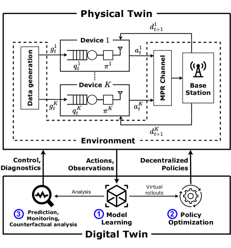
Figure 1: The digital twin (DT) platform for the control and analysis of the communication system studied in this work. The physical twin (PT) consists of a group of $K$ devices receiving correlated data and communicating over a shared multi-packet reception (MPR) channel. The DT platform operates along the phases of model learning \raisebox{-0.9pt}{1}⃝ and policy optimization \raisebox{-0.9pt}{2}⃝; while also enabling functionalities such as prediction, counterfactual analysis and monitoring \raisebox{-0.9pt}{3}⃝.

A digital twin (DT) platform can be viewed as a cyberphysical system in which a physical entity, referred to as the physical twin (PT), and a virtual model, known as the DT, interact based on an automatized bi-directional flow of information [1, 2]. Based on data received from the PT, the DT maintains an up-to-date model of the PT [3], which is leveraged to control, monitor, and analyze the operation of the PT [4]. DT platforms are increasingly regarded as an enabling technology for wireless cellular systems built on the open networking principles of disaggregation and virtualization [5], which are expected to be central to 6G [6].

This paper introduces a general framework based on Bayesian learning for the design of a DT platform implementing the functions of control and monitoring of a wireless system (see Fig. 1). In the proposed framework, the DT builds a Bayesian model of the system dynamics based on data received from the PT. The model is then leveraged to optimize transmission policies via Bayesian multi-agent reinforcement learning (MARL), while also enabling monitoring for anomaly detection, without the need to integrate additional data from the PT. Unlike standard frequentist models, Bayesian models have the key property of providing an accurate quantification of epistemic uncertainty arising from limited PT-to-DT communication, and hence limited data at the DT. As a possible embodiment of the proposed approach, the DT platform may be implemented as an xApp, or as a collection of connected xApps, that run in the near-real-time RAN Intelligent Controller (RIC) of an Open-RAN (O-RAN) architecture [7].

As an exemplifying case study, we consider a multi-access PT system consisting of a radio access network (RAN) similar to that studied in [8, 9, 10]. It is emphasized that, unlike [8, 9, 10], our goal here is not to address a particular task via MARL, but rather to introduce a general framework supporting the implementation of multiple functionalities at the DT, including control via MARL and monitoring, despite the limited data transfer from the PT to the DT.

I-B Related Work

DT-aided control of PT systems is often formulated as a model-based reinforcement learning (RL) problem in which the DT is leveraged as simulation platform to optimize the PT policy [11, 12, 13]. In [14], a Bayesian model is deployed by the DT to enable the quantification epistemic uncertainty. Existing work on DT platforms for wireless systems has investigated mechanisms for DT-PT synchronization [15] and DT-aided network optimization and monitoring [16], as well as DT-based control for computation offloading via model-based RL [11]. To the best of our knowledge, applications of DT relying on Bayesian learning for communication systems have not been reported in the literature.

I-C Main Contributions

The main contributions of this paper are as follows:

$\bullet$ We propose a Bayesian framework to control and monitor an AI-native wireless system, using a multi-access RAN as an exemplifying case study [8, 9, 10]. In the proposed approach, as illustrated in Fig. 1, a Bayesian model learning phase is followed by policy optimization and monitoring phases, which leverage the uncertainty quantification capacity of Bayesian models.

$\bullet$ A key challenge in the definition of a Bayesian model is the choice of a domain-specific factorization of the joint distribution of all variables of interest. This paper elucidates this design choice for a multi-access system consisting of sensing devices with correlated packet arrivals reporting to a common receiver through a shared multi-packet reception (MPR) channel [17]. This case study is relevant for Internet-of-Things (IoT) and machine-type communications.

$\bullet$ Experimental results confirm the advantages of the proposed Bayesian framework as compared to conventional frequentist model-based approaches in terms of metrics such as throughput and buffer overflow, as well as area under the receiver operating curve (ROC) for anomaly detection at the DT.

II Bayesian DT Framework

In this section, we formally define a PT system comprising multiple network elements, such as mobile devices or infrastructure nodes, referred to as agents. We then present a Bayesian DT framework to estimate the PT dynamics, optimize the agents decisions, and monitor possible anomalies in the PT.

II-A Multi-Agent PT System

The PT system of interest consists of $K$ agents, e.g., $K$ sensing devices, indexed by $k\in\mathcal{K}=\{1,\dots,K\}$ that operate over a discrete time index $t=1,2,\dots$, e.g., over time slots. At each time $t$, each agent takes an action $a^{k}_{t}$, e.g., a decision on whether to transmit a packet from its queue or not. The action is selected by following a policy that leverages information collected by the agent regarding the current state $s_{t}$ of the overall system, which may include include, e.g., packet queue lengths. The state $s_{t}$ evolves according to some ground-truth transition probability $T(s_{t+1}|s_{t},a_{t})$, such that the probability distribution of the next state $s_{t+1}\sim T(s_{t+1}|s_{t},a_{t})$ depends on the current state $s_{t}$ and joint action $a_{t}=(a^{1}_{t},\dots,a^{K}_{t})$. We restrict our framework to the case of jointly observable states [18], in which the state $s_{t}$ can be identified if one has access to all observations $o^{k}_{t}$ made by all agents $k\in\mathcal{K}$ at time $t$, i.e., in which the state is a function of the collection $o_{t}=(o^{1}_{t},\dots,o^{K}_{t})$ for all times $t$.

Agents in the PT cannot communicate, and hence the overall information available at agent $k$ up to time $t$ is contained in its action-observation history $h^{k}_{t}=(o^{k}_{1},a^{k}_{1},o^{k}_{2},\dots,a^{k}_{t-1},o^{k}_{t})$. Accordingly, the behaviour of agent $k$ is defined by its policy $\pi^{k}(a^{k}_{t}|h^{k}_{t})$, which defines the probability of each possible action $a^{k}_{t}$ based on the available information $h^{k}_{t}$.

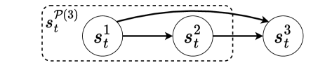
Figure 2: Example of factorization in (1), excluding the variables corresponding to previous time steps $t-1$.

The state of a communication system typically comprises several substates, describing, e.g., the current traffic conditions or the quality of the wireless channel. As a result, one can typically partition the state variables $s_{t}$ into $M$ operationally distinct subsets $\{s^{i}_{t}\}_{i=1}^{M}$ indexed by $i$. To describe the interactions among these subsets, we introduce a Bayesian network defined by a directed acyclic graph, as illustrated in Fig. 2, in which each subset $s^{i}_{t}$ is directly affected by the subset of “parent” variables $s^{\mathcal{P}(i)}_{t}\subseteq s_{t}$ (see, e.g., [19]). Accordingly, the transition probability is assumed to factorize as

$$T\left(s_{t+1}|s_{t},a_{t}\right)=\prod_{i=1}^{M}T^{i}\left(s^{i}_{t+1}\middle|s^{\mathcal{P}(i)}_{t+1},s_{t},a_{t}\right),$$ (1)

where the conditional distribution $T^{i}(s^{i}_{t+1}|s^{\mathcal{P}(i)}_{t+1},s_{t},a_{t})$ describes the evolution of the next states variables $s^{i}_{t+1}$ given the current state $s_{t}$, action $a_{t}$, and parent variables $s^{\mathcal{P}(i)}_{t+1}$. In general, the distribution $T^{i}(s^{i}_{t+1}|s^{\mathcal{P}(i)}_{t+1},s_{t},a_{t})$ depends on some sufficient statistic of variables $s_{t}$ and $a_{t}$, which may be a function of subsets of such variables. We refer to Sec. III-A for an instance of model (1).

II-B Model Learning

The goal of the model learning phase (phase \raisebox{-0.9pt}{1}⃝ in Fig. 1) at the DT is to obtain an estimate of the PT system dynamics in (1). To this end, the PT applies a fixed exploration policy $\pi_{e}=\{\pi_{e}^{k}(a^{k}_{t}|h^{k}_{t})\}_{k\in\mathcal{K}}$, and communicates to the DT the experiences $\mathcal{D}^{\pi_{e}}_{T}=\{(s_{\tau},a_{\tau},s_{\tau+1})\}_{\tau<T}$ collected up to some time $t=T$ while following policy $\pi_{e}$.

Using data $\mathcal{D}^{\pi_{e}}_{T}$, the DT optimizes parametric models $T^{i}_{\theta^{i}}(s^{i}_{t+1}|s^{\mathcal{P}(i)}_{t+1},s_{t},a_{t})$ for each of the ground-truth distributions $T^{i}(s^{i}_{t+1}|s^{\mathcal{P}(i)}_{t+1},s_{t},a_{t})$ for $i\in\{1,\dots,M\}$ in (1), yielding the overall model $T_{\theta}(s_{t+1}|s_{t},a_{t})=\prod_{i=1}^{M}T^{i}_{\theta^{i}}(s^{i}_{t+1}|s^{\mathcal{P}(i)}_{t+1},s_{t},a_{t})$. Some of the distributions $T^{i}_{\theta^{i}}(s^{i}_{t+1}|s^{\mathcal{P}(i)}_{t+1},s_{t},a_{t})$ may be known, e.g., those describing the operation of a communication protocol. For such distributions, the DT simply sets $T^{i}(s^{i}_{t+1}|s^{\mathcal{P}(i)}_{t+1},s_{t},a_{t})=T^{i}_{\theta^{i}}(s^{i}_{t+1}|s^{\mathcal{P}(i)}_{t+1},s_{t},a_{t})$. For the unknown factors, the DT adopts a Bayesian learning framework, which aims at evaluating the posterior distributions $P(\theta^{i}|\mathcal{D}^{\pi_{e}}_{T})$ of each model parameter vector $\theta^{i}$ given the available data $\mathcal{D}^{\pi_{e}}_{T}$.

If the observations $\{o^{k}_{t}\}_{k\in\mathcal{K}}$, and hence the state $s_{t}$, take discrete values, the parameters $\theta^{i}$ may be chosen to directly represent the transition distributions. In such case, if the state space is sufficiently small, the exact computation of the posterior can be done using the Dirichlet-Categorical model (see, e.g., [20]). For high dimensional and continuous problems, computing the exact posterior $P(\theta^{i}|\mathcal{D}^{\pi_{e}}_{T})$ is intractable, and the DT must fall back to using function approximation methods such as Bayesian neural networks (BNN), and inference algorithms such as Markov chain Monte Carlo (MCMC), or variational inference [20]. By (1), and assuming that the parameters $\theta^{i}$ are a priori independent, this comes with no loss of optimality.

II-C Policy Optimization

Having obtained the posterior distributions $P(\theta^{i}|\mathcal{D}^{\pi_{e}}_{T})$ for the model parameters, during policy optimization (phase \raisebox{-0.9pt}{2}⃝ in Fig. 1), the DT aims to optimize the decentralized policy $\pi=\{\pi^{k}(a^{k}_{t}|h^{k}_{t})\}_{k\in\mathcal{K}}$ so as to maximize some user-specified performance criterion. This is defined by a reward function $r(s_{t},a_{t},s_{t+1})$, which determines in turn the total discounted return

$$G_{t}=\sum_{\tau=t}^{+\infty}\gamma^{\tau-t}r(s_{\tau},a_{\tau},s_{\tau+1}),$$ (2)

for some exponential discounting factor $\gamma\in[0,1]$ when the PT applies the policy $\pi$. The optimal control problem consists of the maximization of the average long-term reward

$$\max_{\pi}\mathbbm{E}_{\pi}(G_{1}),$$ (3)

which amounts to a Decentralized MDP (Dec-MDP) [18]. We emphasize that the DT has only access to the model $T_{\theta}(s_{t+1}|s_{t},a_{t})$, and not to the ground-truth distribution in (1) when addressing problem (3).

In this work, we implement the COunterfactual Multi-Agent (COMA) algorithm in [21], a state-of-the-art centralized critic with decentralized actors (CCDA) method, to tackle problem (3) by leveraging model-generated virtual rollouts at the DT. In COMA, the DT maintains a centralized critic $Q_{w}(s_{t},a_{t})$, with parameter vector $w$, as well as the decentralized policies $\pi_{v}=\{\pi^{k}_{v}(a^{k}_{t}|h^{k}_{t})\}_{k\in\mathcal{K}}$, with common parameter vector $v$. The parameterized critic $Q_{w}(s_{t},a_{t})$ is optimized to approximate the Q-value $Q^{\pi_{v}}(s_{t},a_{t})=\mathbbm{E}_{\pi_{v}}[G_{t}|s_{t},a_{t}]$ and is used only for policy optimization. Once optimized, each policy $\pi^{k}_{v}$ is transmitted to its respective agent $k$ at the end of the policy optimization phase.

A key distinction between the approach adopted here and the conventional COMA implementation is the fact that the model $T_{\theta}(s_{t+1}|s_{t},a_{t})$ is stochastic with model parameter vector $\theta$ being distributed according to the posterior $P(\theta|\mathcal{D}^{\pi_{e}}_{T})$. In a manner similar to [22], we account for the epistemic uncertainty encoded by the posterior $P(\theta|\mathcal{D}^{\pi_{e}}_{T})$ by periodically sampling a parameter vector $\theta\sim P(\theta|\mathcal{D}^{\pi_{e}}_{T})$ during policy optimization so as to produce the next state $s_{t+1}\sim T_{\theta}(s_{t+1}|s_{t},a_{t})$ in the virtual rollouts.

II-D Monitoring

As an example of functionalities enabled by Bayesian model learning at the DT besides control, we focus here on anomaly detection (phase \raisebox{-0.9pt}{3}⃝ in Fig. 1). Anomaly detection aims at detecting significant changes in the dynamics of the PT. To formulate this problem, we assume that, during the operation of the system following policy optimization (phase \raisebox{-0.9pt}{2}⃝ in Fig. 1), the DT has access to the information $\mathcal{D}^{\pi}_{T^{\mathrm{M}}}=\{(s_{\tau},a_{\tau},s_{\tau+1})\}_{\tau<{T^{\mathrm{M}}}}$ about the state-action sequence experienced by the PT within some time window ${T^{\mathrm{M}}}$ under the optimized policy $\pi$. The DT tests if the collected data $\mathcal{D}^{\pi}_{T^{\mathrm{M}}}$ is consistent with the data reported by the PT during the most recent model learning phase (phase \raisebox{-0.9pt}{1}⃝ in Fig. 1), or rather if it provides evidence of changed conditions or anomalous behavior.

To this end, we adopt a disagreement-based test metric (see, e.g., [23]), which quantifies the level of epistemic uncertainty associated with the reported experience $\mathcal{D}^{\pi}_{T^{\mathrm{M}}}$. We define as

$$LL\left(\mathcal{D}^{\pi}_{T^{\mathrm{M}}}\middle|\theta\right)=\sum_{\tau=1}^{T^{\mathrm{M}}-1}\log\left(T_{\theta}(s_{\tau+1}|s_{\tau},a_{\tau})\pi(a_{\tau}|s_{\tau})\right)$$ (4)

the log-likelihood of model $\theta$ for the reported experience $\mathcal{D}^{\pi}_{T^{\mathrm{M}}}$, where $\pi(a_{\tau}|s_{\tau})=\prod_{k\in\mathcal{K}}\pi^{k}(a^{k}_{\tau}|h^{k}_{\tau})$. We then consider the test metric is given by the variance

$$\mathbbm{E}_{P(\theta|\mathcal{D}^{\pi_{e}}_{T})}\left[\left(LL\left(\mathcal{D}^{\pi}_{T^{\mathrm{M}}}\middle|\theta\right)-\mathbbm{E}_{P(\theta|\mathcal{D}^{\pi_{e}}_{T})}\left[LL\left(\mathcal{D}^{\pi}_{T^{\mathrm{M}}}\middle|\theta\right)\right]\right)^{2}\right],$$ (5)

estimated using samples from distribution $P(\theta|\mathcal{D}^{\pi_{e}}_{T})$. A larger variance provides evidence of a large epistemic uncertainty, which is taken to indicate an anomalous observation $\mathcal{D}^{\pi}_{T^{\mathrm{M}}}$ as compared to the model learning conditions.

III Multi-Access System Case Study

In order to illustrate the operation and the benefits of the proposed framework for the implementation of a DT platform, in the rest of the paper we focus on a multi-access IoT-like wireless network as the PT system to be controlled and monitored [8, 9, 10].

III-A Setting

As illustrated in Fig. 1, the PT system under study comprises $K$ sensing devices that obtain data with correlated data arrivals both in time [24] and across devices [8], and communicate with a common base station (BS) over an unknown MPR channel [17]. With $t$ denoting the time slot index, and following the notation in Sec. II, each device $k\in\mathcal{K}$ observes $o^{k}_{t}=(q^{k}_{t},g^{k}_{t},d^{k}_{t})$, where $q^{k}_{t}\in\{0,1,\dots,Q^{k}_{\mathrm{max}}\}$ is the number of packets in the device buffer; $g^{k}_{t}\in\{0,1\}$ is a binary variable indicating if a new packet is generated ($g^{k}_{t}=1$) at time $t$ or not ($g^{k}_{t}=0$); and $d^{k}_{t}\in\{0,1\}$ indicates whether a packet sent at the previous time step $t-1$ from device $k$ was successfully delivered at the BS ($d^{k}_{t}=1$) or not ($d^{k}_{t}=0$). The state of the PT is represented by the joint observation of all devices, $s_{t}=o_{t}=(o^{1}_{t},\dots,o^{K}_{t})$.

The access policy of device $k$ is given by the distribution $\pi^{k}(a^{k}_{t}|h^{k}_{t})$, where we have $a^{k}_{t}=1$ if the device attempts to transmit the first packet in its buffer, and $a^{k}_{t}=0$ if it stays idle in slot $t$. Finally, we define the (binary) packet-generation vector as $g_{t}=(g^{1}_{t},\dots,g^{K}_{t})$, the successful packet-delivery vector as $d_{t}=(d^{1}_{t},\dots,d^{K}_{t})$, and the packet-transmission vector as $a_{t}=(a^{1}_{t},\dots,a^{K}_{t})$.

In the O-RAN implementation mentioned in Sec. I-A, communication between the PT and the DT occurs on the E2 interface, with each device $k$ communicating its observations $o^{k}_{t}$ to the RIC, and the DT feeding back the transmission policies $\{\pi^{k}(a^{k}_{t}|h^{k}_{t})\}_{k\in\mathcal{K}}$ to the corresponding devices through the relevant distributed unit [7].

As we will detail next, and as an instance of (1), the ground-truth transition dynamics can be factorized as

$$\begin{split}T(s_{t+1}|s_{t},a_{t})=&P(g_{t+1}|g_{t})\times P(d_{t+1}|a_{t})\times\\ &\prod_{k\in\mathcal{K}}P(q^{k}_{t+1}|q^{k}_{t},d^{k}_{t+1},g^{k}_{t+1}),\end{split}$$ (6)

where $P(g_{t+1}|g_{t})$ describes the packet-generation process; the distribution $P(d_{t+1}|a_{t})$ describes the shared access channel; and $P(q^{k}_{t+1}|q^{k}_{t},d^{k}_{t+1},g^{k}_{t+1})$ describes the (deterministic) buffer update rule.

The packet generation mechanism is modelled as a correlated Markovian process with transition probability distribution $P(g_{t+1}|g_{t})$. To account for spatial correlation, we partition the devices into clusters $\{\mathcal{C}^{i}\}_{i=1}^{C}$ with $\mathcal{C}^{i}\subseteq\mathcal{K}$, $\mathcal{C}^{i}\cap\mathcal{C}^{j}=\emptyset$ if $i\neq j$ and $\bigcup_{i=1}^{C}\mathcal{C}^{i}=\mathcal{K}$, where each cluster $\mathcal{C}^{i}$ contains devices with correlated packet arrivals. Accordingly, the data-generation dynamics factorize without loss of generality as

$$P(g_{t+1}|g_{t})=\prod_{i=1}^{C}P\left(g^{\mathcal{C}^{i}}_{t+1}\middle|g^{\mathcal{C}^{i}}_{t}\right),$$ (7)

where $g^{\mathcal{C}^{i}}_{t}=\{g^{k}_{t}\}_{k\in\mathcal{C}^{i}}$ for $i\in\{1,\dots,C\}$.

Each device $k$ maintains a first-in first-out buffer of maximum capacity $Q^{k}_{\mathrm{max}}$, where the buffer state $q^{k}_{t}$ evolves according to the deterministic update $P(q^{k}_{t+1}|q^{k}_{t},d^{k}_{t+1},g^{k}_{t+1})$ given by

$$q^{k}_{t+1}=\min(Q^{k}_{\mathrm{max}},q^{k}_{t}+g^{k}_{t+1}-d^{k}_{t+1}).$$ (8)

If device $k$ generates a new packet when the buffer is full and transmission fails, i.e., if we have the equalities $q^{k}_{t}=Q^{k}_{\mathrm{max}}$, $g^{k}_{t+1}=1$, and $d^{k}_{t+1}=0$, a buffer overflow event occurs at time step $t+1$. In this case, the oldest packet in the buffer is deleted without being sent, and the newly generated packet at time $t+1$ is added to the buffer as per the update rule in (8).

The transmission probability from the devices to the BS $P(d_{t+1}|a_{t})$ is described by an MPR channel [17]. Accordingly, of the $n^{\mathrm{Tx}}_{t}=\sum_{k\in\mathcal{K}}a^{k}_{t}\in\{1,\dots,K\}$ simultaneously sent packets at time $t$, only $n^{\mathrm{Rx}}_{t+1}=\sum_{k\in\mathcal{K}}d^{k}_{t+1}\in\{0,1,\dots,n^{\mathrm{Tx}}_{t}\}$ are successfully received as the BS. The distribution of the number of received packets $n^{\mathrm{Rx}}_{t+1}$ given $n^{\mathrm{Tx}}_{t}$ is defined by the MPR channel distribution $P(n^{\mathrm{Rx}}_{t+1}|n^{\mathrm{Tx}}_{t})$. The $n^{\mathrm{Rx}}_{t+1}$ successfully received packets are chosen uniformly from the $n^{\mathrm{Tx}}_{t}$ transmissions. Note that the action variable $a^{k}_{t}$ necessarily takes value $a^{k}_{t}=0$ if the buffer is empty, i.e., we have the inequality $a^{k}_{t}\leq q^{k}_{t}$. Furthermore, delivery can be successful only if a packet is transmitted, i.e., we have $a^{k}_{t}\geq d^{k}_{t+1}$. Therefore, the input-output MPR channel distribution relating the packet-transmission vector $a_{t}$ for time $t$ to the successful packet-delivery vector $d_{t+1}$ at time $t+1$ is given by

$$P(d_{t+1}|a_{t})=P(n^{\mathrm{Rx}}_{t+1}|n^{\mathrm{Tx}}_{t})\times\frac{\prod_{k\in\mathcal{K}}\mathbbm{1}_{\left\{a^{k}_{t}\geq d^{k}_{t+1}\right\}}}{\binom{n^{\mathrm{Tx}}_{t}}{n^{\mathrm{Rx}}_{t+1}}}.$$ (9)

For each successfully decoded packet, the BS sends back an acknowledgement (ACK) message to the sending device $k$ over an error-free channel on the control plane. A summary of the notations can be found in the upmost part of Figure 1.

III-B Model Learning

The deterministic queue dynamics (8) and the symmetry of the MPR channel in the rightmost part of (9) are assumed to be known to the DT, so that the DT needs only an estimate of the data generation process distribution $P(g_{t+1}|g_{t})$, and of the MPR channel distribution $P(n^{\mathrm{Rx}}_{t+1}|n^{\mathrm{Tx}}_{t})$. The DT models the $M=C+1$ factors $\{P(g^{\mathcal{C}^{i}}_{t+1}|g^{\mathcal{C}^{i}}_{t})\}_{i=1}^{C}$ and $P(n^{\mathrm{Rx}}_{t+1}|n^{\mathrm{Tx}}_{t})$ using tabular models, and we adopt the Categorical-Dirichlet Bayesian model (see Sec. II-B).

III-C Policy Optimization

In a similar manner to [10], we assume that the reward in (2) takes the form

$$r(s_{t},a_{t},s_{t+1})=\sum_{k\in\mathcal{K}}\beta^{k}r^{k}(o^{k}_{t},a^{k}_{t},o^{k}_{t+1}),$$ (10)

with

$$r^{k}(o^{k}_{t},a^{k}_{t},o^{k}_{t+1})=\left\{\begin{array}[]{ll}+\xi&\mbox{if }d^{k}_{t+1}=1\\ -\xi&\mbox{if }q^{k}_{t}=Q^{k}_{\mathrm{max}}\mbox{, }g^{k}_{t+1}=1\mbox{ and}\\ &d^{k}_{t+1}=0\\ -1&\mbox{otherwise},\end{array}\right.$$ (11)

where the first condition corresponds to successful packet delivery and the second condition to buffer overflow. The constants $\{\beta^{k}\}_{k\in\mathcal{K}}$ and $\xi>0$ are hyperparameters under the control of the network operator at the DT. The average in (3) is taken with respect to the packet-generation process, the MPR channel, and the policy $\pi$, with all buffers initialized as being empty, i.e., $q^{k}_{1}=0$ for all devices $k\in\mathcal{K}$.

The critic $Q_{w}(s_{t},a_{t})$ and the policies $\pi^{k}_{v}(a^{k}_{t}|h^{k}_{t})$ for the COMA algorithm presented in Sec. II-C are implemented as feedforward networks. Specifically, the policy $\pi^{k}_{v}(a^{k}_{t}|h^{k}_{t})$ takes as input its current observation $o^{k}_{t}$, along with the positional input $p_{t}=(t\mod{F})$, where $F$ is a hyperparameter, resulting in a simplified policy $\pi^{k}(a^{k}_{t}|o^{k}_{t},p_{t})$. The adoption of complex policies using recurrent neural networks (RNNs) [25] is left for future work. We refer to the codebase repository [26] for further details on the implementation of policy optimization.

IV Experiments

IV-A Setup and Benchmarks

In this section, we evaluate the proposed DT platform of our case study in a simulated scenario consisting of $K=4$ devices distributed in $C=2$ clusters, with devices $1$ and $2$ in cluster $\mathcal{C}^{1}$, and devices $3$ and $4$ in cluster $\mathcal{C}^{2}$. The per-cluster packet-generation distribution $P(g^{\mathcal{C}^{i}}_{t+1}|g^{\mathcal{C}^{i}}_{t})$ in (7) is such that two devices in the same cluster cannot simultaneously generate a packet, and a new packet is generated at either device with probability $0.4$. Each device $k\in\{1,2,3,4\}$ is equipped with a buffer with capacity $Q^{k}_{\mathrm{max}}=1$ packet, and the reward parameters in (10), (11), and (2) are set to $\beta^{k}=1$ for all $k\in\{1,2,3,4\}$, $\gamma=0.95$, and $\xi=50$.

The MPR channel allows for the successful transmission of a single packet with probability $1$; while, for two simultaneous transmissions, one packet is received with probability 0.8 and both packets are received with probability 0.2. More than two simultaneous transmissions cause the loss of all packets.

The Bayesian model is initialized with all prior Dirichlet parameters equal to $0.01$. As benchmarks, we consider: $(i)$ an oracle-aided model-free policy optimization scheme, in which the policy optimizer is allowed to interact with the ground-truth model (6) until convergence; $(ii)$ a frequentist model-based MARL approach, which obtains a maximum a posteriori (MAP) estimate $\theta^{\mathrm{MAP}}$ of the model parameter vector $\theta$ during model learning with all Dirichlet prior parameters set to $1.01$, guaranteeing well-defined solutions for the MAP problem, and uses the single optimized model $T_{\theta^{\mathrm{MAP}}}(s_{t+1}|s_{t},a_{t})$ for policy optimization and monitoring. For data collection during the model learning phase, we adopt a random exploration policy $\pi_{e}^{k}(a^{k}_{t}=1|h^{k}_{t})=q_{t}$, where probability $q_{t}$ is uniformly and independently selected in the interval $[0,1]$ at each step $t$.

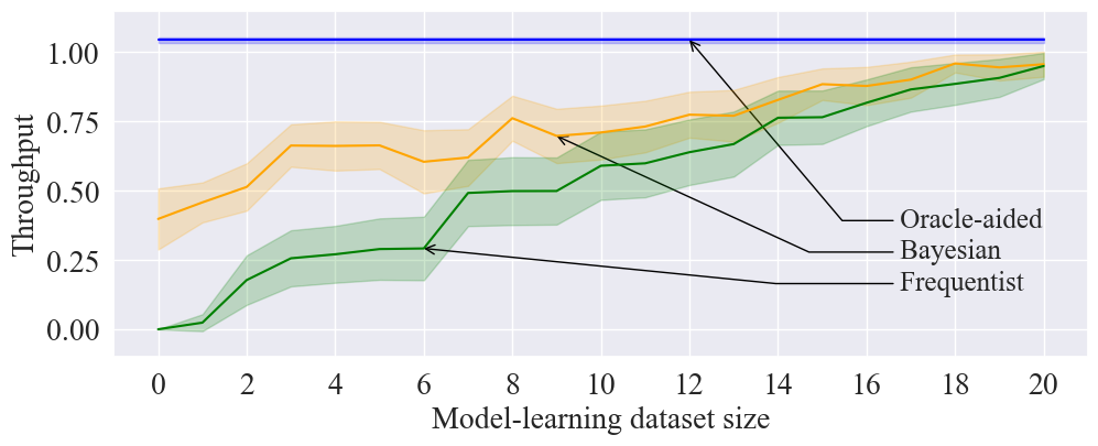
(a)

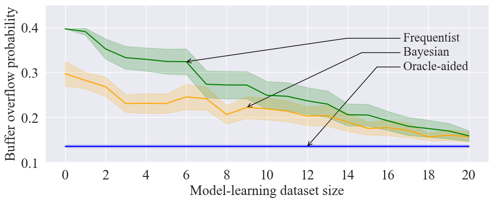
(b)

Figure 3: Throughput (a) and buffer overflow probability (b) as a function of the size of the dataset available in the model learning phase for the proposed Bayesian model-based approach (orange), as well as the oracle-aided model-free (blue) and frequentist model-based (green) benchmarks.

IV-B Policy Evaluation

We evaluate the performance of policy optimization in the ground-truth environment by using the following metrics: the average number of packets successfully sent at each time step, i.e., the throughput (Fig. 3(a)); and the average probability of buffer overflow across all devices (Fig. 3(b)). We focus on the impact of the size of the model learning dataset $\mathcal{D}^{\pi_{e}}_{T}$ by varying the number of exploratory steps $T$ from $0$ to $20$ in the model learning phase. The results are averaged over 50 independent model learning and policy optimization cycles.

From Fig. 3, we observe that, in regimes with high data availability during the model learning phase, i.e., with large $T$, both Bayesian and frequentist model-based methods yield policies with similar performance to the oracle-aided benchmark. In the low-data regime, however, Bayesian learning achieves superior performance compared to its frequentist counterpart. With frequentist learning, which disregards epistemic uncertainty, policy optimization is prone to model exploitation, whereby the optimized policy is misled by model errors into taking actions that are unlikely to be advantageous in the ground-truth dynamics. By using an ensemble of models with distinct transition dynamics in state-action space regions with high epistemic uncertainty, Bayesian learning reduces the sensitivity of the optimized policy to model errors.

IV-C Anomaly Detection

We now consider the performance of anomaly detection by assuming that an anomalous event occurs when device $2$ is disconnected, resulting in an anomalous distribution $P(g^{\mathcal{C}^{1}}_{t+1}|g^{\mathcal{C}^{1}}_{t})$ for which a packet is generated at device $1$ only with probability $0.4$, and no packet is generated at either device in cluster $\mathcal{C}^{1}$ with probability $0.6$. To focus on such anomalies at the packet generation level, we use the log-likelihood $LL^{\mathcal{C}^{1}}(\mathcal{D}^{\pi}_{T^{\mathrm{M}}}|\theta)=\sum_{\tau=1}^{T^{\mathrm{M}}-1}\log(P(g^{\mathcal{C}^{1}}_{\tau+1}|g^{\mathcal{C}^{1}}_{\tau}))$ in place of $LL(\mathcal{D}^{\pi}_{T^{\mathrm{M}}}|\theta)$ in (5). Furthermore, we consider as benchmark a standard test based on the log-likelihood $LL^{\mathcal{C}^{1}}(\mathcal{D}^{\pi}_{T^{\mathrm{M}}}|\theta^{\mathrm{MAP}})$ obtained from MAP-based frequentist learning.

For each model learning dataset size $T=20$ and $T=50$, we report the false positive rates (FPR) and the true positive rates (TPR) of the anomaly detection tests by varying the detection threshold in Fig. 4. Each curve is averaged over $50$ independent model learning phases, while the optimized policy $\pi$ used to report experiences $\mathcal{D}^{\pi}_{T^{\mathrm{M}}}$ remains the same.

Bayesian anomaly detection is observed to uniformly outperform its frequentist counterpart, achieving a higher area under the ROC in Fig. 4. For instance, at a TPR of $0.8$, the Bayesian anomaly detector has a FPR of $0.33$ for a model learning dataset size of $T=20$ and a FPR of $0.15$ for a dataset size of $T=50$; whereas the frequentist benchmark has a FPR of $0.40$ for $T=20$ and $0.28$ for $T=50$. These results suggest that measuring epistemic uncertainty instead of likelihood can yield more effective monitoring solutions.

Figure 4: Receiver operating curves (ROC) of the Bayesian (orange) and frequentist (green) anomaly detection tests. Solid lines represent model learning dataset sizes of $T=20$ steps, while dashed lines correspond to dataset sizes of $T=50$ steps.

V Conclusions

This paper has proposed a Bayesian framework for the development of a DT platform by focusing on a multi-access sensing system as a case study. By accounting for epistemic uncertainty during model learning, the proposed Bayesian DT framework was shown to obtain more reliable control than conventional frequentist counterparts in the low data regime, while also enhancing monitoring functionalities. Future work may investigate the use of more complex policies accounting for partial observability at each agent [25]; and the design of exploration policies for model learning [22].

References

- [1] M. Grieves and J. Vickers, “Digital twin: Mitigating unpredictable, undesirable emergent behavior in complex systems,” in Transdisciplinary perspectives on complex systems. Springer, 2017, pp. 85–113.
- [2] W. Kritzinger, M. Karner, G. Traar, J. Henjes, and W. Sihn, “Digital twin in manufacturing: A categorical literature review and classification,” IFAC-PapersOnLine, vol. 51, no. 11, pp. 1016–1022, 2018.
- [3] E. Glaessgen and D. Stargel, “The digital twin paradigm for future NASA and US Air Force vehicles,” in in Proc. AIAA/ASME/ASCE/AHS/ASC Structures, Structural Dynamics and Materials Conference 20th AIAA/ASME/AHS Adaptive Structures Conference 14th AIAA, 2012, p. 1818.
- [4] P. Almasan, M. Ferriol-Galmés, J. Paillisse, J. Suárez-Varela, D. Perino, D. López, A. A. P. Perales, P. Harvey, L. Ciavaglia, L. Wong et al., “Network digital twin: Context, enabling technologies and opportunities,” arXiv preprint arXiv:2205.14206, 2022.
- [5] A. Akman, C. Li, L. Ong, L. Suciu, B. Sahin, T. Li, P. Stjernholm, J. Voigt, A. Buldorini, Q. Sun et al., “ORAN use cases and deployment scenarios: Towards open and smart RAN,” O-RAN Alliance, White Paper, Feb, 2020.
- [6] L. U. Khan, W. Saad, D. Niyato, Z. Han, and C. S. Hong, “Digital-twin-enabled 6G: Vision, architectural trends, and future directions,” IEEE Communications Magazine, vol. 60, no. 1, pp. 74–80, 2022.
- [7] A. Lacava, M. Polese, R. Sivaraj, R. Soundrarajan, B. S. Bhati, T. Singh, T. Zugno, F. Cuomo, and T. Melodia, “Programmable and customized intelligence for traffic steering in 5G networks using Open RAN architectures,” arXiv, 2022. [Online]. Available: https://arxiv.org/abs/2209.14171
- [8] R. Kassab, A. Destounis, D. Tsilimantos, and M. Debbah, “Multi-agent deep stochastic policy gradient for event based dynamic spectrum access,” in 2020 IEEE 31st Annual International Symposium on Personal, Indoor and Mobile Radio Communications. IEEE, 2020, pp. 1–6.
- [9] A. Valcarce and J. Hoydis, “Toward joint learning of optimal MAC signaling and wireless channel access,” IEEE Transactions on Cognitive Communications and Networking, vol. 7, no. 4, pp. 1233–1243, 2021.
- [10] L. Miuccio, S. Riolo, S. Samarakoon, D. Panno, and M. Bennis, “Learning generalized wireless MAC communication protocols via abstraction,” in GLOBECOM 2022 - 2022 IEEE Global Communications Conference, 2022, pp. 2322–2327.
- [11] Y. Dai, K. Zhang, S. Maharjan, and Y. Zhang, “Deep reinforcement learning for stochastic computation offloading in digital twin networks,” IEEE Transactions on Industrial Informatics, vol. 17, no. 7, pp. 4968–4977, 2020.
- [12] C. Cronrath, A. R. Aderiani, and B. Lennartson, “Enhancing digital twins through reinforcement learning,” in 2019 IEEE 15th International Conference on Automation Science and Engineering (CASE). IEEE, 2019, pp. 293–298.
- [13] X. Wang, L. Ma, H. Li, Z. Yin, T. Luan, and N. Cheng, “Digital twin-assisted efficient reinforcement learning for edge task scheduling,” in 2022 IEEE 95th Vehicular Technology Conference:(VTC2022-Spring). IEEE, 2022, pp. 1–5.
- [14] C. Li, S. Mahadevan, Y. Ling, S. Choze, and L. Wang, “Dynamic Bayesian network for aircraft wing health monitoring digital twin,” Aiaa Journal, vol. 55, no. 3, pp. 930–941, 2017.
- [15] O. Hashash, C. Chaccour, and W. Saad, “Edge continual learning for dynamic digital twins over wireless networks,” arXiv preprint arXiv:2204.04795, 2022.
- [16] L. Hui, M. Wang, L. Zhang, L. Lu, and Y. Cui, “Digital twin for networking: A data-driven performance modeling perspective,” arXiv preprint arXiv:2206.00310, 2022.
- [17] L. Tong, Q. Zhao, and G. Mergen, “Multipacket reception in random access wireless networks: From signal processing to optimal medium access control,” IEEE Communications Magazine, vol. 39, no. 11, pp. 108–112, 2001.
- [18] F. A. Oliehoek and C. Amato, A concise introduction to decentralized POMDPs. Springer, 2016.
- [19] D. Koller and N. Friedman, Probabilistic graphical models: principles and techniques. MIT press, 2009.
- [20] O. Simeone, Machine Learning for Engineers. Cambridge University Press, 2022.
- [21] J. Foerster, G. Farquhar, T. Afouras, N. Nardelli, and S. Whiteson, “Counterfactual multi-agent policy gradients,” in Proceedings of the AAAI conference on artificial intelligence, vol. 32, no. 1, 2018.
- [22] Q. Zhang, C. Lu, A. Garg, and J. Foerster, “Centralized model and exploration policy for multi-agent RL,” arXiv preprint arXiv:2107.06434, 2021.
- [23] E. Daxberger and J. M. Hernández-Lobato, “Bayesian variational autoencoders for unsupervised out-of-distribution detection,” arXiv preprint arXiv:1912.05651, 2019.
- [24] N. Nikaein, M. Laner, K. Zhou, P. Svoboda, D. Drajic, M. Popovic, and S. Krco, “Simple traffic modeling framework for machine type communication,” in ISWCS 2013; The Tenth International Symposium on Wireless Communication Systems. VDE, 2013, pp. 1–5.
- [25] P. Zhu, X. Li, P. Poupart, and G. Miao, “On improving deep reinforcement learning for POMDPs,” arXiv preprint arXiv:1704.07978, 2017.
- [26] C. Ruah, “Bayesian Digital Twin Repository,” 2022. [Online]. Available: https://github.com/kclip/bayesian-dt