Higher Order Far-Field Boundary Conditions
for Crystalline Defects

Abstract.

Lattice defects in crystalline materials create long-range elastic fields that can be modelled on the atomistic scale. The low rank structures of defect configurations are revealed by a rigorous far-field expansion of the long-range elastic fields [3], and thus the defect equilibrium can be expressed as a sum of continuum correctors and discrete multipole terms that are essentially computable. In this paper, we develop a novel family of numerical schemes that exploit the multipole expansions to accelerate the simulation of crystalline defects. In particular, the relatively slow convergence rate of the standard cell approximations for defect equilibration could be significantly developed. To enclose the simulation in a finite domain, a theoretically justified approximation of multipole tensors is therefore introduced, which leads to a novel moment iteration as well as the higher order boundary conditions. Moreover, we consider a continuous version of multipole expansions to acquire efficiency in practical implementation. Several prototypical numerical examples of point defects are presented to test the convergence for both geometry error and energy error. The numerical results show that our proposed numerical scheme can achieve the accelerated convergence rates in terms of computational cell size with the higher order boundary conditions.

1. Introduction

Determining the geometry and energies of defects in crystalline solids play a central role in computational materials science [14, 15, 28, 34]. The crystalline defects generally distort the host lattice, resulting in the long-range elastic fields that can be modelled on the atomistic scale. Molecular simulation provides a typical and accurate methodology to study complex material behaviour with defects at the nano-scale, whereas the field of continuum solid mechanics has already gained great success in supplying robust predictions of material behaviour at the macro-scale. Connecting discrete and continuous models of materials to predict and compute defect behaviour in crystals, has since been developed and attracted great attentions over the past half century [5, 11, 20, 29].

A key approximation in all numerical simulations of crystalline defects is the boundary condition since practical schemes necessarily work in small computational domains. Hence, one can not explicitly resolve crystalline far-field but must employ artificial boundary conditions (e.g., clamped or periodic boundary conditions [4, 12]). The quality of boundary conditions has a significant consequence for the severity of cell-size effects in such simulations. A critical challenge is to develop higher order boundary conditions such that the improved accuracy can be systematically achieved.

Toward that end, one common approach is to characterize the elastic fields surrounding the defect core, leveraging the low rank structures of defect configurations. Modelling defects in continuum linear elasticity (CLE) by employing the defect dipole tensor (also known as the elastic dipole tensor or the double force tensor) is originated by [13, 22]. The applications on the atomistic models of fracture are then proposed in [26, 27]. More recent related works include that of Trinkle and coworkers, where lattice Green’s functions have been used to improve the accuracy of defect computations [30, 31]. The initial concept of far-field expansion of the elastic-fields in a simplified setting is explored in [2].

Recently, Braun et.al [3] unifies many of the ideas involved in those previous works into a single framework and expands them systematically to higher orders. To be more precise, the defect equilibrium can be expressed as a sum of continuum correctors and discrete multipole terms encapsulated by the spatial moments of acting forces. The relative simplicity of these moments provides an elegant and computable approach to transfer information from the nonlinear discrete problem to the continuum hierarchy. More importantly, a sequence of smooth predictors which describe the far-field behaviour of the lattice strain around a defect within arbitrary accuracy is constructed, and thus provides increasingly accurate boundary conditions to be used on the discrete model when confined to a finite domain. In particular, this work could be used as a foundation for a rigorous numerical analysis of defect algorithms and also demonstrate a path to systematically improve their accuracy.

The purpose of the present work is to develop a novel family of numerical schemes that exploit the multipole expansions to accelerate the simulation of crystalline defects. As a critical application of the previous theoretical work [3], the proposed numerical scheme accelerates the approximate cell problems that leverage the explicit low-dimensional structure of defect fields. In particular, the slow convergence rates of the standard cell approximations for defect equilibration problem initiated in [12] could be systematically improved. As briefly mentioned in [3], the main challenge for constructing the practical schemes is that the multipole moments terms cannot be evaluated since it is defined on the infinite lattice. Hence, an approximate evaluation of the exact multipole tensors have to be engaged in when confined to a finite computational domain. We give a rigorous error estimate of the moment errors arising from this approximation, which depends on the corresponding geometry error itself with certain rate of convergence in terms of computational cell size. This result not only motivates us to fulfill accelerated convergence of cell problems in practical implementation by applying a novel moment iteration, but also leads to robust new numerical schemes and analysis of defect dipole tensor (also called the elastic dipole tensor) specifically. Such schemes are of important and ongoing interest in defect physics (e.g., [10, 21]). In particular, our approach to these terms developed here naturally includes the anisotropic case as well as extensions to higher multipole tensors. A continuous multipole expansion that employs the continuous Green’s functions is utilized to provide an efficient implementation. We finally conduct the moment iteration for several prototypical numerical examples of point defects to test the convergence of both geometry error and energy error. The numerical results show that the proposed numerical scheme can achieve the accelerated convergence rates in terms of computational cell size by providing the higher order boundary conditions.

In the present paper we mainly constrain ourselves to the point defects to clearly present the main ideas, and the generalization of this work would be investigated in depth in the future. We note that, even an extension to other “simple defects” such as straight dislocation lines appears less straightforward. In more complex scenarios, such as curved dislocations or extrapolating on grain boundary structures with distinct coordination environment there are fundamental challenges that our analysis does not cover even heuristically and requires significant additional ideas.

Outline

The paper is organized as follows: In Section 2, we describe the variational formulation for the equilibration of crystalline defects and review the results on multipole expansions (cf. [3, Theorem 3.1]), which gives the general structure results on characterisations of the discrete elastic far-fields surrounding point defects. In Section 3, as an immediate application of the defect expansions, we develop a novel family of numerical schemes exploiting the multipole expansions to accelerate the simulation of crystalline defects with a theoretically justified approximation of the moment tensors. The main moment iteration algorithm (cf. Algorithm 3.1) is therefore designed. This approach can in principle improve the poor convergence rates of standard cell approximations for the defect equilibration problem. In Section 4, we first consider the continuous multipole expansions instead of the discrete one to give an efficient implementation. We then conduct the continuous moment iteration (cf. Algorithm 4.2) for several prototypical numerical examples of point defects to give a numerical verification. In Section 5, we provide a summary and outlook. The proofs of main theorem and the further analysis of additional issues that are helpful to understand the main ideas of this paper are given in Section 6. We also provide a supplementary part containing some further details in Section 7.

Notation

We use the symbol $\langle\cdot,\cdot\rangle$ to denote an abstract duality pairing between a Banach space and its dual space. The symbol $|\cdot|$ normally denotes the Euclidean or Frobenius norm, while $\|\cdot\|$ denotes an operator norm. We denote $A\backslash\{a\}$ by $A\backslash a$, and $\{b-a~{}|~{}b\in A\}$ by $A-a$. For $E\in C^{2}(X)$, the first and second variations are denoted by $\langle\delta E(u),v\rangle$ and $\langle\delta^{2}E(u)v,w\rangle$ for $u,v,w\in X$.

Given a $k$-tuple of vectors in $\mathbb{R}^{d}$, $\bm{\sigma}=(\sigma^{(1)},\dots,\sigma^{(k)})\in(\mathbb{R}^{d})^{k}$, we write the $k$-fold tensor product as

$$\bm{\sigma}^{\otimes}:=\bigotimes_{i=1}^{k}\sigma^{(i)}:=\sigma^{(1)}\otimes\cdots\otimes\sigma^{(k)}.$$

The vector space spanned by these tensor products is denoted by $(\mathbb{R}^{d})^{\otimes k}$, and it is easy to see this space is isomorphic to $\mathbb{R}^{d^{k}}$. Similarly, we write $v^{\otimes k}:=v\otimes...\otimes v\in(\mathbb{R}^{d})^{\otimes k}$ when considering the $k$-fold tensor product of a single vector $v\in\mathbb{R}^{d}$.

For any $\bm{\sigma}\in(\mathbb{R}^{d})^{k}$, we define the symmetric tensor product by

$$\bm{\sigma}^{\odot}:=\sigma^{(1)}\odot\cdots\odot\sigma^{(k)}:={\rm sym~{}}\bm{\sigma}^{\otimes}:=\frac{1}{k!}\sum_{g\in S_{k}}g(\bm{\sigma})^{\otimes},$$

where $S_{k}$ is the usual symmetric group of all permutations acting on the integers $\{1,\ldots,k\}$ and $g(\bm{\sigma}):=(\sigma^{(g(1))},\dots,\sigma^{(g(k))})$ for any $g\in S_{k}$ and $\bm{\sigma}\in(\mathbb{R}^{d})^{k}$. The space spanned by these symmetric tensors is then denoted by $(\mathbb{R}^{d})^{\odot k}$, and thus is a vector subspace of $(\mathbb{R}^{d})^{\otimes k}$.

The natural scalar product on $(\mathbb{R}^{d})^{\otimes k}$ and $(\mathbb{R}^{d})^{\odot k}$ is denoted by $A:B$ for $A,B\in(\mathbb{R}^{d})^{\otimes k}$, which is defined to be the linear extension of

$$\bm{\sigma}^{\otimes}:\bm{\rho}^{\otimes}:=\prod_{i=1}^{k}\sigma^{(i)}\cdot\rho^{(i)}.$$

For two second-order tensors ${\bf C},{\bf U}\in(\mathbb{R}^{A})^{\otimes k}$, given specifically as a sum ${\bf C}=\sum_{\bm{\rho}\in A^{k}}{\bf C}_{\bm{\rho}}E_{\bm{\rho}}$ with $E_{\bm{\rho}}$ the natural basis of the space ${\mathbb{R}^{d}}^{k}$, we can then write

$${\bf C}\colon{\bf U}=\sum_{\bm{\rho}\in A^{k}}{\bf C}_{\bm{\rho}}{\bf U}_{\bm{\rho}}.$$

We write $|A|\lesssim B$ if there exists a constant $C$ such that $|A|\leq CB$, where $C$ may change from one line of an estimate to the next. When estimating rates of decay or convergence, $C$ will always remain independent of the system size, the configuration of the lattice and the the test functions. The dependence of $C$ will be normally clear from the context or stated explicitly.

2. Background: Equilibration of crystalline defects and its multipole expansions

Our results are concerned with modelling of crystalline defects, i.e., a single point defect embedded in a homogeneous crystalline bulk. For the sake of brevity of presentation, the single-species Bravais lattices are mainly considered, and we note that the algorithms proposed in this work can be applied to multilattice crystals [23] with suitable modifications on the notations only. We briefly review the setting of various previous works [7, 12, 17] to motivate the formulation of our main results in this context, and then give a brief summary of the theory proposed in [3], which can be regarded as important background for our own work.

2.1. Equilibration of crystalline point defects

Given $d\in\{2,3\}$, $\mathsf{A}\in\mathbb{R}^{d\times d}$ non-singular. Let $\Lambda:=\mathsf{A}\mathbb{Z}^{d}$ be a Bravais lattice possessing no defects, and $\Lambda^{\rm def}\subset\mathbb{R}^{d}$ be the reference configuration with point defect satisfying $\exists~{}R^{\rm def}>0$, such that $\Lambda^{\rm def}\backslash B_{R^{\rm def}}=\Lambda\backslash B_{R^{\rm def}}$ and $\Lambda^{\rm def}\cap B_{R^{\rm def}}$ is finite.

For different types of point defects, for example, allowing $\Lambda^{\rm def}\neq\Lambda$ in $B_{R^{\rm def}}$ admits defects such as vacancies and interstitials, whereas allowing inhomogeneity of $V_{\ell}$ admits impurities and foreign interstitials.

The displacement of the infinite lattice $\Lambda$ is a map $u\colon\Lambda\to\mathbb{R}^{N}$, where we allow $N\neq d$ in order to model a range of scenarios. For $\ell,\rho\in\Lambda$, we denote discrete differences by $D_{\rho}u(\ell):=u(\ell+\rho)-u(\ell)$. To introduce higher discrete differences we denote by $D_{\bm{\rho}}=D_{\rho_{1}}\cdots D_{\rho_{j}}$ for a $\bm{\rho}=(\rho_{1},...,\rho_{j})\in\Lambda^{j}$. For a subset $\mathcal{R}_{\ell}\subset\Lambda-\ell$, we define $D_{\mathcal{R}_{\ell}}u(\ell):=\big{(}D_{\rho}u(\ell)\big{)}_{\rho\in\mathcal{R}_{\ell}}$. We assume throughout that $\mathcal{R}_{\ell}$ is finite for each site $\ell\in\Lambda$. The extension to infinite interaction range requires substantial technicalities, see [7] and references therein for a possible remedy.

The discrete energy space $\mathcal{H}^{1}$ is defined by

$$\mathcal{H}^{1}(\Lambda^{\rm def})=\big{\{}u:\Lambda^{\rm def}\to\mathbb{R}^{N}~{}\big{|}~{}\|u\|_{\mathcal{H}^{1}}:=\|Du\|_{\ell^{2}}<\infty\big{\}}.$$

For future reference we also define the dense subspace $\mathcal{H}^{\rm c}\subset\mathcal{H}^{1}$ of displacements with compact support,

$$\mathcal{H}^{\rm c}(\Lambda^{\rm def})=\big{\{}u:\Lambda^{\rm def}\to\mathbb{R}^{N}~{}\big{|}~{}{\rm supp}(Du)\text{~{}bounded~{}}\big{\}}.$$

$\mathcal{H}^{1}(\Lambda)$ and $\mathcal{H}^{\rm c}(\Lambda)$ can be analogously defined for displacements on homogeneous lattice.

We consider the site potential to be a collection of mappings $V_{\ell}:(\mathbb{R}^{N})^{\mathcal{R}_{\ell}}\rightarrow\mathbb{R}$, which represent the energy distributed to each atomic site. We make the following assumption on regularity and symmetry: $V_{\ell}\in C^{K}((\mathbb{R}^{N})^{\mathcal{R}_{\ell}})$ for some $K$ and $V_{\ell}$ is homogeneous outside the defect region $B_{R^{\rm def}}$, namely, $V_{\ell}=V$ and $\mathcal{R}_{\ell}=\mathcal{R}$ for $\ell\in\Lambda\setminus B_{R^{\rm def}}$. Furthermore, $V$ and $\mathcal{R}$ have the following point symmetry: $\mathcal{R}=-\mathcal{R}$, it spans the lattice $\textrm{span}_{\mathbb{Z}}\mathcal{R}=\Lambda$, and $V(\{-A_{-\rho}\}_{\rho\in\mathcal{R}})=V(A)$.

We define the discrete difference stencil $Du(\ell):=D_{\mathcal{R}}u(\ell)$ for notational convenience. Moreover, the higher discrete differences (applying the operator $D$ for $k$ times) will be considered for which we utilise the simple notation $D^{k}u:=D\cdots Du\in\mathbb{R}^{N}\otimes(\mathbb{R}^{\mathcal{R}})^{\otimes k}$.

The potential energy under a displacements $u:\Lambda^{\rm def}\to\mathbb{R}^{d}$ and $u:\Lambda\to\mathbb{R}^{d}$ are then, respectively, given by

(2.1) $$\mathcal{E}^{\rm def}(u):=\sum_{\ell\in\Lambda^{\rm def}}\Big{[}V_{\ell}\big{(}D_{\mathcal{R}_{\ell}}u(\ell)\big{)}-V_{\ell}\big{(}{\bf 0}\big{)}\Big{]},\qquad\mathcal{E}(u):=\sum_{\ell\in\Lambda}\Big{[}V\big{(}Du(\ell)\big{)}-V\big{(}{\bf 0}\big{)}\Big{]}.$$

We note that $\mathcal{E}$ is well defined on $\mathcal{H}^{\rm c}$ and has a unique continuous extension to $\mathcal{H}^{1}$. The same is true with $\mathcal{E}^{\rm def}$ for analogously defined $\mathcal{H}^{\rm c}(\Lambda^{\rm def})$ and $\mathcal{H}^{1}(\Lambda^{\rm def})$. Furthermore with $V\in C^{K}$ we also find $\mathcal{E},\mathcal{E}^{\rm def}\in C^{K}$, all of which is shown in [12, Lemma 1].

At the most fundamental level, we concern the characterisation of the far-field behaviour of lattice displacements $u:\Lambda\to\mathbb{R}^{N}$ that are close to equilibrium in the far-field. According to [3], it is important to characterise the linearised residual forces $f(\ell):=H[u](\ell)$, where

(2.2) $$H[u](\ell):=-{\rm Div}~{}\big{(}\nabla^{2}V({\bf 0})[Du]\big{)},$$

with ${\rm Div}~{}A=-\sum_{\rho\in\mathcal{R}}D_{-\rho}A_{\cdot\rho}$ the discrete divergence for a matrix field $A\colon\Lambda\to\mathbb{R}^{N\times\mathcal{R}}$.

If $\ell\mapsto H[u](\ell)\otimes\ell^{\otimes i}\in\ell^{1}(\Lambda)$, we define the $i$-th (force) moment

(2.3) $$\mathcal{I}_{i}[u]=\sum_{\ell\in\Lambda}H[u](\ell)\otimes\ell^{\otimes i}.$$

A point defect can be thought of as a finite-energy equilibrium of $\mathcal{E}$, that is, the equilibrium displacements $\bar{u}^{\rm def}\in\mathcal{H}^{1}(\Lambda^{\rm def})$ satisfy

(2.4) $$\delta\mathcal{E}^{\rm def}(\bar{u}^{\rm def})[v]=0\qquad\forall v\in\mathcal{H}^{\rm c}(\Lambda^{\rm def}).$$

In order to give the following analysis, it is convenient to project $\bar{u}^{\rm def}$ to the homogeneous lattice $\Lambda$. The possible projections are not unique, for example, for single vacancy, we can define $\bar{u}:\Lambda\to\mathbb{R}^{d}$ by

$$\bar{u}(\ell):=\begin{cases}\bar{u}^{\rm def}(\ell),&\ell\in\Lambda\cap\Lambda^{\rm def},\\[4.30554pt] 0,&\ell\in\Lambda\setminus\Lambda^{\rm def}.\end{cases}$$

For interstitial, $\bar{u}(\ell):=\bar{u}^{\rm def}(\ell),~{}\ell\in\Lambda$. We remark that the subsequent results are essentially independent of how this projection is performed.

2.2. Multipole expansions of equilibrium

In this section, we briefly introduce the multipole expansions result of the equilibrium $\bar{u}$ for point defects. Due to the fact that $\bar{u}=\bar{u}^{\rm def}$ outside the defect core, for $\lvert\ell\rvert$ large enough, we obtain that

$$\delta\mathcal{E}(\bar{u})(\ell)=\delta\mathcal{E}(\bar{u})[\delta_{\ell}]=0,$$

where $\delta_{\ell}(\ell^{\prime}):=\delta_{\ell\ell^{\prime}}$. As a matter of fact, with a small amount of additional work one can show

$$\delta\mathcal{E}(\bar{u})[v]=(g,Dv)_{\ell^{2}}\qquad\forall v\in\mathcal{H}^{1}(\Lambda),$$

where $g:\Lambda\to\mathbb{R}^{d\times\mathcal{R}}$ with ${\rm supp}(g)\subset B_{R^{\rm def}}$. Next, we state the following result originating from [3, Theorem 3.1], which gives the general structure results on characterisations of the discrete elastic far-fields surrounding crystalline point defects.

Theorem 2.1.

Choose $p\geq 0,J\geq 0$ and suppose that $V\in C^{K}(\mathbb{R}^{d\times\mathcal{R}})$, such that $K\geq J+2+\max\{0,\lfloor\frac{p-1}{d}\rfloor\}$. Let $g:\Lambda\to\mathbb{R}^{d\times\mathcal{R}}$ with compact support, and let $\bar{u}\in\mathcal{H}^{1}(\Lambda)$ such that

$$\delta\mathcal{E}(\bar{u})[v]=(g,Dv)_{\ell^{2}}\quad\forall v\in\mathcal{H}^{\rm c}(\Lambda).$$

Furthermore, let $\mathcal{S}\subset\Lambda$ be linear independent with ${\rm span}_{\mathbb{Z}}\mathcal{S}=\Lambda$. Then, there exist $u_{i}^{C}\in C^{\infty}$ and coefficients $b_{\rm exact}^{(i,k)}\in(\mathbb{R}^{\mathcal{S}})^{\odot i}$ such that

(2.5) $$\bar{u}=\sum_{i=d+1}^{p}u_{i}^{C}+\sum_{i=1}^{p}\sum_{k=1}^{N}b_{\rm exact}^{(i,k)}:D_{\rm\mathcal{S}}^{i}\mathcal{G}_{k}+r_{p+1},$$

and such that the $u_{i}^{C}$ satisfy the PDEs in [3, Eq.(59)] with $u_{i}^{C}=0$ for $0\leq i\leq d$. Furthermore, for $j=1,\dots,J$, the remainder term $r_{p+1}$ satisfies the estimate

(2.6) $$\lvert D^{j}r_{p+1}\rvert\lesssim\lvert\ell\rvert^{1-d-j-p}\log^{p+1}(\lvert\ell\rvert).$$

Remark 2.1.

We have three comments on Theorem 2.1 that would be helpful to understand the motivation and main ideas of this paper:

(1) Since $u_{i}^{C}=0$ for $0\leq i\leq d$, we have the pure multipole expansion up to order $p=d$

(2.7) $$\bar{u}=\sum_{i=1}^{d}\sum_{k=1}^{N}b_{\rm exact}^{(i,k)}:D_{\rm\mathcal{S}}^{i}\mathcal{G}_{k}+r_{d+1},\ \text{where}\ \lvert D^{j}r_{d+1}\rvert\lesssim\lvert\ell\rvert^{1-2d-j}\log^{d+1}(\lvert\ell\rvert).$$

Moreover, as discussed in [3, Remark 3.4], it is possible to reduce the number of logarithms in the estimate somewhat for all orders in (2.6) and (2.7). Nevertheless, we still choose to keep them since they will not influence the primary theory and algorithms proposed in this work essentially.

(2) The coefficients $b_{\rm exact}^{(i,k)}$ can be obtained through a linear relation (cf. [3, Lemma 5.6]) from the force moments defined by (2.3), that is,

(2.8) $$\big{(}\mathcal{I}_{i}(\bar{u})\big{)}_{\cdot k}=(-1)^{i}i!\sum_{\bm{\rho}\in\mathcal{S}^{i}}(b^{(i,k)}_{\rm exact})_{\bm{\rho}}\cdot\bm{\rho}^{\odot}.$$

See also Section 6.2 for a detailed derivation (cf. Eq.(6.2)) for $i=1,2,3$.

(3) To give an efficient implementation, we avoid having to work with the discrete Green’s functions and their discrete derivatives. As a matter of fact, the connection between the continuous and the discrete Green’s functions has been proposed in [3, Theorem 2.5 and Theorem 2.6]. Hence, instead of dealing with the discrete coefficients $b^{(i,k)}_{\rm exact}$ shown in (2.7), a pure continuous expansion of $\bar{u}$ with respect to the continuous Green’s functions (the corresponding coefficients are denoted by $a^{(i,n,k)}$) should be considered. We leave the detailed constructions in Section 4.1.

3. Practical numerical scheme: Moment iteration

3.1. Accelerated convergence of cell problems

An immediate application of the defect expansions (cf. Theorems 2.1) is that it suggests a novel family of numerical schemes that exploit the multipole expansions to accelerate the simulation of crystalline defects. These approaches can in principle improve the relatively slow convergence rates of standard cell approximations for the defect equilibration problem (2.4) established in [12]. In this section, we first review the pure Galerkin approximation scheme of cell problems proposed in [3] and then discuss its limitations, which prevent it from the practical simulation.

Toward that end, we define a family of restricted displacement spaces

(3.9) $$\mathcal{W}_{R} :=\big{\{}v:\Lambda\to\mathbb{R}^{N}~{}\big{|}~{}v(\ell)=0\text{ for $|\ell|>R$}\big{\}},$$

(3.10) $$\mathcal{U}_{R} :=\big{\{}u=u_{0}^{C}+v~{}\big{|}~{}v\in\mathcal{W}_{R}\big{\}},$$

where atoms are clamped in their reference configurations outside a ball with radius $R$. Then we can approximate (2.4) by the Galerkin projection as follows

(3.11) $$\delta\mathcal{E}(\bar{u}_{R})[v]=0\qquad\forall v\in\mathcal{W}_{R},$$

where $\bar{u}_{R}\in\mathcal{U}_{R}$.

Under suitable stability conditions it is shown in [12] that

(3.12) $$\|D\bar{u}_{R}-D\bar{u}\|_{\ell^{2}}\leq CR^{-d/2},$$

for $R$ sufficiently large. It is crucial to underline that this convergence is an immediate corollary of the decay estimate $|Dr_{1}(\ell)|\lesssim\lvert\ell\rvert^{-d}\log^{p}(\lvert\ell\rvert)$ (let $p=0$ in (2.6)). Our overarching goal in this work is to propose a novel numerical scheme aiming to accelerate this relatively slow convergence with an improved far-field boundary condition by exploiting the multipole expansion presented in Theorem 2.1.

The main idea is to

1. replace the naive far-field predictor $\hat{u}_{0}:=0$ for point defects with the higher-order predictor

   $$\hat{u}_{p}:=\sum_{i=0}^{p}u_{i}^{\rm C},$$

   where $u_{i}^{\rm C}$ are the solutions of the PDEs given in [3, Eq. (59)]. Note that $u^{\rm C}_{i}$ for $0\leq i\leq d$ for point defects.

2. enlarge the admissible corrector space with the multipole moments

   $$\mathcal{U}_{R}^{(p)}:=\big{\{}v:\Lambda\to\mathbb{R}^{N}\,\big{|}\, \,\,v=\sum_{i=1}^{p}\sum_{k=1}^{N}b^{(i,k)}_{\rm exact}:D^{i}_{\mathcal{S}}\mathcal{G}_{k}+w,$$

   $$\text{for free coefficients $b^{(i,k)}_{\rm exact}$ and ${\rm supp}~{}w\subset\Lambda\cap B_{R}$ }\big{\}}.$$

   That is, the corrector displacement is now parametrised by its values in the computational domain $\Lambda\cap B_{R}$ and by the discrete coefficients $b^{(i,k)}_{\rm exact}$ of the multipole terms.

Hence, we can consider the pure Galerkin approximation scheme: Find $\bar{v}_{R}\in\mathcal{U}^{(p)}_{R}$, $\bar{u}_{p,R}=\hat{u}_{p}+\bar{v}_{R}$, such that

(3.13) $$\delta\mathcal{E}(\bar{u}_{p,R})[v_{R}]=0\qquad\forall v_{R}\in\mathcal{W}_{R}.$$

The arguments of [12] leading to (3.12) are generic Galerkin approximation arguments, leveraging the strong stability condition. They can be followed verbatim up to the intermediate result (Céa’s Lemma)

$$\big{\|}D\bar{u}-D\hat{u}_{p}-D\bar{v}_{R}\big{\|}_{\ell^{2}}\leq C\inf_{v_{R}\in\mathcal{U}_{R}^{(p)}}\big{\|}D\bar{u}-D\hat{u}_{p}-Dv_{R}\big{\|}_{\ell^{2}}.$$

The existence of $\bar{v}_{R}$ is implicitly guaranteed through an application of the inverse function theorem (cf. Lemma 6.1), since the right-hand side in this estimate (i.e., consistency) approaches zero as $R\to\infty$. To estimate the right-hand side we can insert the exact tensors $b^{(i,k)}_{\rm exact}$ from the solution representation of Theorems 2.1 into $v_{R}$, in order to obtain $D\bar{u}-D\hat{u}_{p}-Dv_{R}=Dr_{p+1}-Dw_{R}$, where $r_{p+1}$ is the core remainder term, and hence

$$\inf_{v_{R}\in\mathcal{U}_{R}}\big{\|}D\bar{u}-D\bar{u}_{p,R}\big{\|}_{\ell^{2}}\leq\inf_{w_{R}\in\mathcal{U}_{R}}\big{\|}Dr_{p+1}-Dw_{R}\big{\|}_{\ell^{2}},$$

Let $w_{R}$ be a suitable truncation of $r_{p+1}$ to the computational domain $B_{R}$. We have the following Theorem, which essentially follows from [12, Theorem 2] but we adapt it the setting considered in this work for both geometry error and energy error.

Theorem 3.1.

Suppose that $\bar{u}$ is a strongly stable solution of (2.4); that is, there exists a stability constant $c_{0}>0$ such that

$$\delta^{2}\mathcal{E}(\bar{u})[v,v]\geq c_{0}\|Dv\|^{2}_{\ell^{2}},\qquad\forall v\in\mathcal{H}^{1}(\Lambda),$$

then, for $R$ sufficiently large, there also exists a solution $\bar{u}_{R}\in\mathcal{U}_{R}^{(p)}$ to the Galerkin scheme (3.13) such that

(3.14) $$\big{\|}D\bar{u}-D\bar{u}_{p,R}\big{\|}_{\ell^{2}} \leq C_{p}R^{-d/2-p}\log^{p+1}(R),$$

(3.15) $$\big{|}\mathcal{E}(\bar{u})-\mathcal{E}(\bar{u}_{p,R})\big{|} \leq C_{E}R^{-d-2p}\log^{2p+2}(R).$$

Proof.

The error estimate for the geometry error follows directly from [3, Theorem 3.7]. We are now giving the error estimate for the energy error. To that end, since $\mathcal{E}$ is twice differentiable along the segment $\{(1-s)\bar{u}+s\bar{u}_{p,R}~{}|~{}s\in(0,1)\}$, we have

$$\big{|}\mathcal{E}(\bar{u})-\mathcal{E}(\bar{u}_{p,R})\big{|} =\Big{|}\int_{0}^{1}\big{\langle}\delta\mathcal{E}\big{(}(1-s)\bar{u}+s\bar{u}_{p,R}\big{)},\bar{u}-\bar{u}_{p,R}\big{\rangle}\,{\textrm{d}}s\Big{|}$$

(3.16) $$\leq CM\big{\|}D\bar{u}-D\bar{u}_{p,R}\big{\|}_{\ell^{2}}^{2},$$

where $M$ is the uniform Lipschitz constant of $\delta\mathcal{E}$. This yields the stated results. ∎

The foregoing Theorem establishes a key theoretical benchmark, providing an ideal error estimate of the accelerated convergence of cell problems. However, due to the reasons that will be discussed below, it cannot be employed in practical implementation.

Remark 3.1.

The scheme (3.13) cannot be implemented as is since the energy difference functional cannot be evaluated for a displacement with infinite range, that is, the multipole tensors $b_{\rm exact}^{(i,\cdot)}$ cannot be evaluated exactly. However, this highly idealised scheme is of immense theoretical value in that it highlight what could potentially be achieved if this challenge can be overcome. Any practical scheme will necessarily have to engage in the approximate evaluation of the exact multipole tensors $b^{(i,\cdot)}_{\rm exact}$, which will be explored in the forthcoming section.

3.2. Calculation of the multipole moments

To address the issue highlighted in Remark 3.1, we adjust our computational scheme from pure Galerkin approximation (3.13) to the one that evaluates the multipole tensors or corresponding moments on a finite domain. To that end, let us keep the multipole tensors in the corrector space fixed beforehand rather than leaving them arbitrary:

$$\mathcal{U}_{b,R}^{(p)}:=\big{\{}v:\Lambda\to\mathbb{R}^{N}\,\big{|}\,\,\,v=\sum_{i=1}^{p}\sum_{k=1}^{N}b^{(i,k)}:D^{i}_{\mathcal{S}}\mathcal{G}_{k}+w,\quad\text{for ${\rm supp}~{}w\subset\Lambda\cap B_{R}$ }\big{\}}.$$

Let $b$ and $b_{\rm exact}$ be the collections of tensors $b^{(i,k)}$ and $b^{(i,k)}_{\rm exact}$ for all possible $i,k$. We note that $b$ are usually different from $b_{\rm exact}$. If we now look for a solution in $\mathcal{U}_{b,R}^{(p)}$ for some given $b$, we will then obtain a specific variant of Theorem 3.1. The proof is similar to that of Theorem 3.1 by considering the difference of moments additionally, so we omit it here for simplicity.

Lemma 3.1.

Suppose that $\bar{u}$ is a strongly stable solution of (2.4). Then, for $R$ sufficiently large, there exists a solution $\bar{u}_{b,R}=\hat{u}_{p}+\bar{v}_{b,R}$, $\bar{v}_{b,R}\in\mathcal{U}_{b,R}^{(p)}$ to (3.13) such that

(3.17) $$\big{\|}D\bar{u}-D\bar{u}_{b,R}\big{\|}_{\ell^{2}}\leq C_{p}R^{-d/2-p}\log^{p+1}(R)+\sum_{i=1}^{p}\lvert b^{(i,\cdot)}-b_{\rm exact}^{(i,\cdot)}\rvert\cdot R^{1-d/2-i}.$$

For convenience of notation, we will drop the subscript $R$ to use $\bar{u}_{b}$, $\bar{v}_{b}$, $\mathcal{U}_{b}^{(p)}$ instead of $\bar{u}_{b,R}$, $\bar{v}_{b,R}$, $\mathcal{U}_{b,R}^{(p)}$ when there is no confusion in the context.

Next, we want to use the current solution $\bar{u}_{b}$ to calculate a better approximation of $b_{\rm exact}$. To be more precise, one can use an iteration starting at $b=0$ to improve the accuracy of $b$ systematically. This approach will result in the fast convergence of $\lvert b^{(i,\cdot)}-b_{\rm exact}^{(i,\cdot)}\rvert$ for all $i$ such that the error $R^{-d/2-p}\log^{p+1}(R)$ is the dominant term in (3.17). Therefore, the optimal convergence rate stated in Theorem 2.1 could be obtained in this way.

In order to approximate $b^{(i,\cdot)}_{\rm exact}$ we turn to consider the force moments $\mathcal{I}_{i}$ instead due to their linear relation (2.8). Let $\eta_{R}:\Lambda\rightarrow\mathbb{R}$ be a smooth cut-off function such that $\eta_{R}=1$ for $\lvert\ell\rvert\leq R/3$, $\eta_{R}=0$ for $\lvert\ell\rvert>2R/3$ and $\lvert\nabla^{j}\eta_{R}\rvert\leq C_{j}R^{-j}$ for $0\leq j\leq 3$. Then, we define the truncated version of the force moments (2.3) as

(3.18) $$\mathcal{I}_{i,R}[u]:=\sum_{\ell\in\Lambda}\big{(}H[u](\ell)\otimes\ell^{\otimes i}\big{)}\cdot\eta_{R}(\ell).$$

For $1\leq i\leq p$, the approximation of the $i$-th moment is denoted by $\mathcal{I}_{i,R}[\bar{v}_{b}]$ whereas the exact $i$-th moment is denoted as $\mathcal{I}_{i}[\bar{v}]$ with $\bar{u}=\hat{u}_{p}+\bar{v}$. The error to the exact force moment is therefore $\big{\lvert}\mathcal{I}_{i,R}[\bar{v}_{b}]-\mathcal{I}_{i}[\bar{v}]\big{\rvert}$ for $1\leq i\leq p$.

We have the following Theorem, which gives a sharp error estimate of this moment error. We only sketch out the proof in the main context for the sake of brevity of presentation. The detailed proof will be given in Section 6.1.

Theorem 3.2.

Under the conditions of Theorem 3.1, for $1\leq i\leq p$, we have

(3.19) $$\big{\lvert}\mathcal{I}_{i,R}[\bar{v}_{b}]-\mathcal{I}_{i}[\bar{v}]\big{\rvert}\lesssim R^{i-1-p}\log^{p}(R)+R^{i-1}\lVert D\bar{v}_{b}-D\bar{v}\rVert_{\ell^{2}}^{2}+\alpha_{i}(R)\lVert D\bar{v}_{b}-D\bar{v}\rVert_{\ell^{2}},$$

where the coefficients $\alpha_{i}(R)$ for $i=1,\ldots,p$ are given by

$$\alpha_{i}(R):=\begin{cases}1&i<1+d/2,\\ \log(R)&i=1+d/2,\\ R^{i-1-d/2}&i>1+d/2.\end{cases}$$

Sketch of the proof.

We split the target moment error $\big{\lvert}\mathcal{I}_{i,R}[\bar{v}_{b,R}]-\mathcal{I}_{i}[\bar{v}]\big{\rvert}$ into two parts. The first part originates from the truncation of moments that can be directly bounded by $\big{\lvert}\mathcal{I}_{i,R}[\bar{v}]-\mathcal{I}_{i}[\bar{v}]\big{\rvert}\lesssim R^{i-p-1}\log^{p}(R)$. The second part arises from the difference between $\bar{v}$ and $\bar{v}_{b}$ measured in the energy norm, which can be estimated by comparing their linearised residual forces. The details are given in Section 6.1. ∎

The foregoing Theorem plays a crucial role in this work since: (1) it leads to a robust new numerical scheme and analysis for the defect dipole tensor ($i=2$, also called the elastic dipole tensor) specifically. Such scheme is of important and ongoing interest in defect physics (e.g., [10, 21]), and our approach naturally includes the extensions to the higher multipole (e.g., tripole and quadrupole) tensors; (2) it demonstrates that the moment errors depend on the corresponding geometry error itself with certain rate of convergence in terms of computational cell size. This result motivates us to fulfill accelerated convergence of cell problems in practical implementation, by applying a novel moment iteration that will be introduced in the next section.

3.3. The moment iteration

In this section, we combine the Galerkin scheme stated in Lemma 3.1 with Theorem 3.2 to compute the force moment iteratively. The following Algorithm shows that the desired accuracy asserted in Theorem 3.1 could be systematically achieved after several steps of moment iteration.

Algorithm 3.1 Moment iteration

Prescribe $p,d,m=0,b^{(i,\cdot)}_{0}=0$ for all $1\leq i\leq p$.

1:  repeat

2:      Evaluate: Given $b_{m}^{(i,\cdot)}$ compute $\bar{v}_{b_{m}}$ in the sense of Theorem 3.1. Compute the resulting moments $\mathcal{I}_{i,R}[\bar{v}_{b_{m}}]$.

3:      Update: Construct new coefficients $b_{m+1}^{(i,\cdot)}$ with $\mathcal{I}_{i,R}[\bar{v}_{b_{m}}]$ by (2.8). Apply Lemma 3.2 to estimate the accuracy of $b_{m+1}^{(i,\cdot)}$. $m=m+1$.

4:  until 

(3.20) $$\lvert b_{m}^{(i,\cdot)}-b_{\rm exact}^{(i,\cdot)}\rvert=O\big{(}R^{i-1-p}\log^{p+1}(R)\big{)}\qquad\textrm{for all}~{}1\leq i\leq p.$$

Let $M=m$. For each $m\leq M$, save $b_{m}$ as a collection of $b_{m}^{(i,\cdot)}$ for all $i$.

Taking into account the estimates (3.17) and (3.19), the stopping criterion (3.20) ensures that

$$\lVert D\bar{u}-D\bar{u}_{b_{M}}\rVert_{\ell^{2}}\leq C_{p}R^{-d/2-p}\log^{p+1}(R),$$

where $\bar{u}_{b_{M}}=\hat{u}_{p}+\bar{v}_{b_{M}}$ with $\bar{v}_{b_{M}}\in\mathcal{U}_{b_{M}}^{(p)}$ the solution to (3.13). This is the optimal estimate of the geometry error for cell problems that can be obtained (cf. Theorem 3.1). The corresponding convergence rate for energy error can be achieved analogously by applying the technique used in proving Theorem 3.1. To be more precise, we have the following Corollary.

Corollary 3.1.

Under the conditions of Theorem 3.1, if $b_{M}$ is a collection of $b^{(i,\cdot)}_{M}$ constructed by the Algorithm 3.1 for all $1\leq i\leq p$, then for $R$ sufficiently large, there also exists a corrector $\bar{u}_{b_{M}}=\hat{u}_{p}+\bar{v}_{b_{M}}$ with $\bar{v}_{b_{M}}\in\mathcal{U}_{b_{M}}^{(p)}$ the solution to (3.13) such that

(3.21) $$\lVert D\bar{u}-D\bar{u}_{b_{M}}\rVert_{\ell^{2}} \leq C_{p}R^{-d/2-p}\log^{p+1}(R).$$

(3.22) $$\big{|}\mathcal{E}(\bar{u})-\mathcal{E}(\bar{u}_{b_{M}})\big{|} \leq C_{E}R^{-d-2p}\log^{2p+2}(R).$$

We note that the number of iterative steps $M$ in Algorithm 3.1 can be determined a priori based on the estimates in Theorem 3.1 and (3.19). It is straightforward to see that the stopping criterion (3.20) can be satisfied after at most $p$ iterations of moment, which means that the number of iteration steps has the trivial upper bound, namely $|M|\leq p$.

Remark 3.2 (A 3D example for $p=3$.).

We give a concrete example of Algorithm 3.1 to illustrate the results shown in Corollary 3.1. We choose $d=3$ and $p=3$, in this case the predictor $\hat{u}_{p}=0$, hence the correctors satisfy $\bar{u}_{b_{i}}=\bar{v}_{b_{i}}$ for all $1\leq i\leq 3$. We make full use of this case throughout the numerical tests in Section 4. The computational procedure is summarized as follows.

Step 1. Let $b_{0}^{(1,\cdot)}=b_{0}^{(2,\cdot)}=b_{0}^{(3,\cdot)}=0$. Compute the zeroth order corrector $\bar{u}_{b_{0}}$. Theorem 3.1 tells us that

$$\lVert D\bar{u}-D\bar{u}_{b_{0}}\rVert_{\ell^{2}}\lesssim R^{-3/2}.$$

Step 2. Evaluate $b^{(i,\cdot)}_{1}$ based on $\mathcal{I}_{i,R}[\bar{v}_{b_{0}}]$ for $i=1,2,3$ by (2.8). Theorem 3.2 gives

$$\lvert b_{1}^{(1,\cdot)}-b_{\rm exact}^{(1,\cdot)}\rvert\lesssim R^{-3/2},\quad\lvert b_{1}^{(2,\cdot)}-b_{\rm exact}^{(2,\cdot)}\rvert\lesssim R^{-3/2},\quad\lvert b_{1}^{(3,\cdot)}-b_{\rm exact}^{(3,\cdot)}\rvert\lesssim R^{-1}\log^{4}(R),$$

where the estimate for $b_{1}^{(3,\cdot)}$ has already obtained the desired accuracy. Compute the first order corrector $\bar{u}_{b_{1}}$. Theorem 3.1 shows

$$\lVert D\bar{u}-D\bar{u}_{b_{1}}\rVert_{\ell^{2}}\lesssim R^{-3}.$$

Step 3. Evaluate $b^{(i,\cdot)}_{2}$ based on $\mathcal{I}_{i,R}[\bar{v}_{b_{1}}]$ for $i=1,2,3$ by (2.8). Theorem 3.2 gives

$$\lvert b_{2}^{(1,\cdot)}-b_{\rm exact}^{(1,\cdot)}\rvert\lesssim R^{-3}\log^{4}(R),\quad\lvert b_{2}^{(2,\cdot)}-b_{\rm exact}^{(2,\cdot)}\rvert\lesssim R^{-2}\log^{4}(R),\quad\lvert b_{2}^{(3,\cdot)}-b_{\rm exact}^{(3,\cdot)}\rvert\lesssim R^{-1}\log^{4}(R),$$

where all of them have the desired accuracy. The stopping criterion (3.20) is therefore satisfied. Compute the second order corrector $\bar{u}_{b_{2}}$. Theorem 3.1 gives

$$\lVert D\bar{u}-D\bar{u}_{b_{2}}\rVert_{\ell^{2}}\lesssim R^{-9/2}\log^{4}(R).$$

Hence, the optimal convergence of the geometry error for $d=3,p=3$ is achieved by applying two iterations of moments ($M=2$). The construction and the error estimates presented above will be numerically verified in Section 4.3.

4. Numerical experiments

In this section, we conduct the moment iteration (Algorithm 3.1) for several prototypical numerical examples of point defects to obtain boundary conditions with significantly improved convergence rates in terms of computational cell size.

4.1. Continuous and discrete coefficients of multipole expansion

As briefly mentioned in Remark 2.1, in practical implementation it is convenient to have a continuum reformulation of the multipole expansion (cf. Theorem 2.1), to avoid having to work with the discrete Green’s function $\mathcal{G}_{i}$ and its discrete derivatives. Hence, we mainly focus on the continuous Green’s functions $G_{i}$ and their continuous derivatives in this section.

Towards that end, following the theory in [3], we could exploit the connections between continuous and discrete Green’s functions and derive higher order continuum approximations of the discrete Green’s function to obtain the continuum Green’s functions $G_{i}$ and their derivatives. If we also use Taylor expansion to get actual derivatives we could get a pure continuum multipole expansion as follows. Though it has been proposed in [3, Theorem 4], we still state it here for the sake of completeness.

Lemma 4.1.

Under the conditions of Theorem 2.1, there exist $a^{(i,n,k)}\in(\mathbb{R}^{d})^{\odot i}$ such that

(4.23) $$\bar{u}=\sum_{k=1}^{N}\sum_{n=0}^{\big{\lfloor}\frac{p-1}{2}\big{\rfloor}}\sum_{i=0}^{p-1-2n}a^{(i,n,k)}:\nabla^{i}(G_{n})_{\cdot k}+w$$

and for $j=1,2$, $\alpha\in\mathbb{N}_{0}$, the remainder decays as

(4.24) $$\lvert D^{j}w\rvert\lesssim{\ell}^{2-d-p-j}\log^{\alpha+1}(\lvert\ell\rvert).$$

The Lemma above shows that we could turn to deal with the coefficients $a^{(i,n,k)}$ for continuous multipole expansions instead of solving the coefficients $b^{(i,k)}$ for discrete multipole expansions (cf. Remark 3.2(3)). Taking into account (2.5) with (4.23), we can obtain the concrete relation between $a^{(i,n,k)}$ and $b^{(i,k)}$ by exploiting the Taylor expansion of discrete difference stencil. See Section 6.2 for a detailed derivation. For $1\leq i,k\leq 3$ and $n=0,1$, the relation is summarized as follows:

$$(a^{(1,0,k)})_{\cdot j} =(a^{(1,1,k)})_{\cdot j}=\sum_{\rho\in\mathcal{R}}(b^{(1,k)})_{\rho}\cdot\rho_{j},$$

(4.25) $$(a^{(2,0,k)})_{\cdot jm} =\sum_{\rho,\sigma\in\mathcal{R}}(b^{(2,k)})_{\rho\sigma}\cdot\rho_{j}\sigma_{m}+\frac{1}{2}\sum_{\rho\in\mathcal{R}}(b^{(1,k)})_{\rho}\cdot\rho_{j}\rho_{m}$$

$$(a^{(3,0,k)})_{\cdot jmn} =\sum_{\rho,\sigma,\tau\in\mathcal{R}}(b^{(3,k)})_{\rho\sigma\tau}\cdot\rho_{j}\sigma_{m}\tau_{n}+\frac{1}{2}\sum_{\rho,\sigma\in\mathcal{R}}(b^{(2,k)})_{\rho\sigma}\cdot(\rho_{j}\sigma_{m}\sigma_{n}+\rho_{j}\rho_{m}\sigma_{n})$$

$$\qquad\qquad\qquad+\frac{1}{6}\sum_{\rho\in\mathcal{R}}(b^{(1,k)})_{\rho}\cdot\rho_{j}\rho_{m}\rho_{n}.$$

As a direct consequence, combining the above identities with (2.8), we can also obtain the relation between the continuous coefficients and moments. As a matter of fact, for each $i$ and $n$, if we denote $a^{(i,n,\cdot)}$ as a collection of $(a^{(i,n,k)})_{\cdot j}$ for all $j,k$, then we have

$$a^{(1,0,\cdot)} =-\mathcal{I}_{1}[\bar{u}],\quad a^{(1,1,\cdot)}=-\mathcal{I}_{1}[\bar{u}],$$

(4.26) $$a^{(2,0,\cdot)} =\frac{1}{2}\mathcal{I}_{2}[\bar{u}],\quad a^{(3,0,\cdot)}=-\frac{1}{6}\mathcal{I}_{3}[\bar{u}],$$

which essentially gives a practical computation of continuous coefficients $a^{(i,n,\cdot)}$ via force moments. We leave the detailed derivations in Section 6.2 for the sake of brevity of presentation. Furthermore, it is crucial to emphasize that the moment iterations proposed in the previous section are still applied for the continuous coefficients $a^{(i,n,\cdot)}$ due to their linear relationship stated in (4.1). Hence, a continuous version of Algorithm 3.1 (cf. Algorithm 4.2) will be proposed in the following.

As the continuous coefficients $a^{(i,n,\cdot)}$ can be directly computed by applying (4.1), we then introduce the corresponding continuous version of Algorithm 3.1 that will be utilized throughout our numerical tests.

Algorithm 4.2 Computation of the higher order correctors

1:  Initialize $u^{0}_{\rm ff}=0$. Compute the zeroth order corrector $\bar{u}_{b_{0}}$ with the zeroth order far-field predictor $u^{0}_{\rm ff}$. The convergence $\lVert D\bar{u}-D\bar{u}_{b_{0}}\rVert_{\ell^{2}}\lesssim R^{-3/2}$ is then obtained.

2:  Evaluate $a^{(1,0)}_{1},a^{(1,1)}_{1},a^{(2,0)}_{1},a^{(3,0)}_{1}$ by applying (4.1). Compute the first order far-field predictor by Lemma 4.1 with $u=u^{0}_{\rm ff}+\bar{u}_{b_{0}}$

$$u^{1}_{\rm ff}:=a^{(1,0)}_{1}:\nabla G_{0}+a^{(1,1)}_{1}:\nabla G_{1}+a^{(2,0)}_{1}:\nabla^{2}G_{0}+a^{(3,0)}_{1}:\nabla^{3}G_{0}.$$

3:  Compute the first order corrector $\bar{u}_{b_{1}}$ with $u^{1}_{\rm ff}$. The corresponding convergence should be $\lVert D\bar{u}-D\bar{u}_{b_{1}}\rVert_{\ell^{2}}\lesssim R^{-3}$.

4:  Evaluate $a^{(1,0)}_{2},a^{(1,1)}_{2},a^{(2,0)}_{2},a^{(3,0)}_{2}$ by applying (4.1). Compute the second order far-field predictor by Lemma 4.1 with $u=u^{1}_{\rm ff}+\bar{u}_{b_{1}}$

$$u^{2}_{\rm ff}:=a^{(1,0)}_{2}:\nabla G_{0}+a^{(1,1)}_{2}:\nabla G_{1}+a^{(2,0)}_{2}:\nabla^{2}G_{0}+a^{(3,0)}_{2}:\nabla^{3}G_{0}.$$

5:  Compute the second order corrector $\bar{u}_{b_{2}}$ with $u^{2}_{\rm ff}$, which achieves the desired accuracy if we ignore the logarithms temporarily, namely $\lVert D\bar{u}-D\bar{u}_{b_{2}}\rVert_{\ell^{2}}\lesssim R^{-9/2}$.

Compared with Algorithm 3.1, Algorithm 4.2 not only serves as a concrete robust approach to obtain the correctors with optimal accelerate convergence rate, but it clarifies the construction of different orders of boundary conditions (predictors). Though we only include the estimated convergence of geometry error in this Algorithm, the convergence of energy error could be estimated directly by applying

(4.27) $$|\mathcal{E}(\bar{u})-\mathcal{E}(\bar{u}_{b_{i}})\big{|}\lesssim\lVert D\bar{u}-D\bar{u}_{b_{i}}\rVert^{2}_{\ell^{2}}\qquad\textrm{for}~{}0\leq i\leq 2.$$

In practical implementation, the continuous Green’s function $G_{0}$ and its first order correction $G_{1}$ are computed by applying the Barnett’s formula [1], of which a rigorous derivation is given in Section 6.3. The higher order derivatives of $G_{0}$ up to the third order, namely $\nabla^{j}G_{0}$, $j=1,2,3$, are obtained using the technique of automatic differentiation [25].

4.2. Model problems

In this section, we conduct the computations of accelerated convergence of cell problems for several typical types of point defects, exploiting the moment iteration (Algorithm 3.1) proposed in the previous section. The extension to dislocations requires additional challenging steps (see Section 5 for a brief discussion), hence we postpone it to a separate work.

We use tungsten (W) in all numerical experiments, which has a body-centred cubic (BCC) crystal structure in the solid state. The embedded atom model (EAM) potential [9] is used to model the interatomic interaction. The cut-off radius is chosen as $r_{\rm cut}=5.5$Å, which includes up to the third neighbour interaction. To avoid the boundary effects, we introduce several layers of clamped ghost atoms whose thickness are greater than $r_{\rm cut}$ outside of the domain of interest.

We consider five prototypical examples of localised point defects; their core geometry (in a 2D slice from the top of view) are visualised in Figure 4.1:

• Single-vacancy (Figure 4.1a): a single vacancy located at the origin; defined by $\Lambda^{\rm def}:=\Lambda\setminus\{{\bm{0}}\}$;

• Di-vacancy (Figure 4.1b): two adjacent vacancies;

• Interstitial (Figure 4.1c): an additional W atom located at the centre of a bond between two nearest neighbors; defined by $\Lambda^{\rm def}:=\Lambda\cup\{(r_{0}/4,r_{0}/4,r_{0}/4)\}$, where $r_{0}$ is the lattice constant of W;

• Micro-crack-2 (Figure 4.1d): a row of five adjacent vacancies;

• Micro-crack-3 (Figure 4.1e): a row of seven adjacent vacancies.

It is worthwhile mentioning that these two micro-crack cases are not technically “cracks”, which in fact serve as the examples of a localized defect with an anisotropic shape. In this section, we mainly present the results of the first three cases for the sake of brevity of presentation. Analogous studies for these two micro-crack cases obtain very similar results, and we therefore leave them to the supplementary part (cf. Section 7).

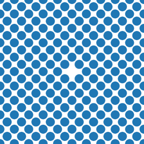
(a) Vacancy

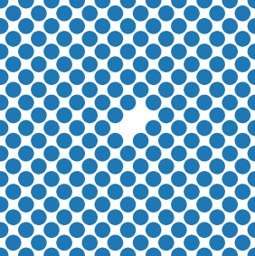
(b) Divacancy

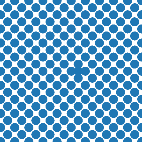
(c) Interstitial

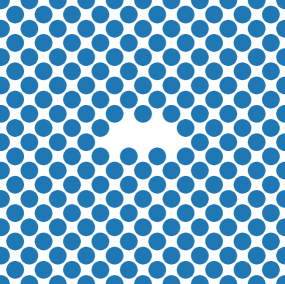
(d) Micro-crack-2

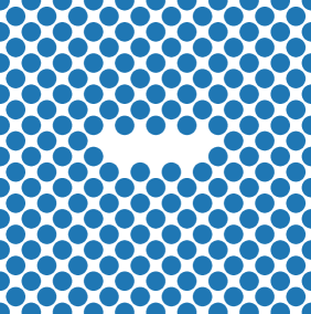
(e) Micro-crack-3

Figure 4.1. Defect cores for the five cases considered in this work, serving as benchmark problems for the numerical tests.

To compute the equilibrium displacement of (2.4) in considerably high accuracy, we employ a preconditioned LBFGS algorithm [19] and then post-processing with a standard Newton scheme. The minimization is terminated at the force residual in $\ell^{\infty}$-norm of $10^{-8}$, that is, $|\nabla\mathcal{E}(u)|_{\infty}<{\rm tol}=10^{-8}$.

4.3. Convergence of cell problems

As discussed in the previous sections, we have already shown that how to exploit the moment iteration to construct boundary conditions systematically such that a significantly improved convergence rate in terms of computational cell size of cell problems is achieved. This in fact serves as a central motivation for the present work. The improved rates of convergence can be obtained without too much increase in computational complexity.

Towards that end, we will perform the convergence studies for both geometry error $\|D\bar{u}-D\bar{u}_{b_{i}}\|_{\ell^{2}}$ and energy error $\big{|}\mathcal{E}(\bar{u})-\mathcal{E}(\bar{u}_{b_{i}})\big{|}$ by increasing the radius of computational domain $R$. The approximate equilibrium $\bar{u}_{b_{i}}$ for $i=0,1,2$ are obtained iteratively by the moment iteration (see Algorithm 3.1 and Remark 3.2). The reference solution $\bar{u}$ is taken to be a numerical solution on a much larger domain with radius $R_{\rm dom}=100r_{0}$ with $r_{0}$ the lattice constant of W.

Moments convergence

First of all, we present the convergence of force moments. The relative error of the $k$-th moment evaluated at $\bar{u}_{b_{i}}$ is given by

(4.28) $${\rm ME}_{ki}:=\frac{\big{|}\mathcal{I}_{k}[\bar{u}_{b_{i}}]-\mathcal{I}_{k}[\bar{u}]\big{|}}{\big{|}\mathcal{I}_{k}[\bar{u}]\big{|}},$$

where $\mathcal{I}_{k}$ is the $k$-th moment defined by (2.3). Figure 4.2 plots the convergence of moments error (4.28) with $i=0,1$ and $k=1,2,3$ against the domain size $R$ for vacancy, divacancy and interstitial, confirming the estimate shown in Theorem 3.2 (or equivalent Remark 3.2). The corresponding results for two micro-crack cases are given by Figure 7.6 in Section 7.2. This result also numerically indicates that the desired accelerated convergence rate could be systematically obtained after several steps of moment iteration.

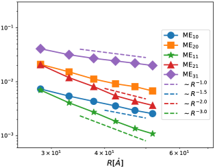
(a) Vacancy

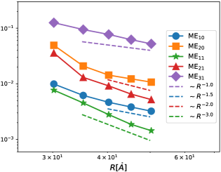
(b) Di-vacancy

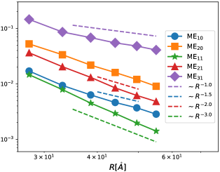
(c) Interstitial

Figure 4.2. Convergence of the relative moments error ${\rm ME}_{ki}$ defined by (4.28) against domain size $R$ for vacancy, di-vacancy and interstitial.

Geometry error

The most valuable observation that illustrates the significance of the current work can be concluded in Figure 4.3, plotting the convergence of geometry error $\|D\bar{u}-D\bar{u}_{b_{i}}\|_{\ell^{2}}$ for $i=0,1,2$ against the domain size $R$ for the first three defect cases considered in this paper. Again, the similar results of micro-cracks are shown in Section 7.2 for simplicity of presentation. Figure 4.3 demonstrates the improved rates of convergence with increasingly accurate boundary conditions by applying moment iteration, which are consistent with our theoretical prediction (cf. Corollary 3.1). It is worthwhile mentioning that the higher order convergence rate can only be observed clearly when $R$ is larger than $30\mathring{\mathrm{A}}$. This problem becomes more crucial when the electronic structure calculation is considered due to the prohibitive computational cost. Though it is beyond the scope of the current work, a future study of combining the current scheme with the flexible boundary conditions [6] might address this issue.

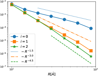
(a) Vacancy

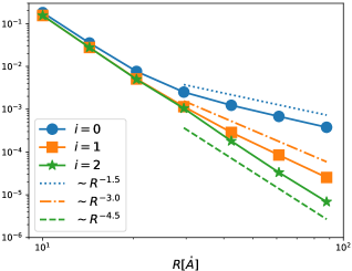
(b) Di-vacancy

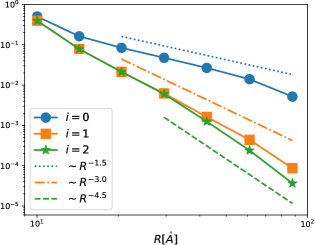
(c) Interstitial

Figure 4.3. Convergence of geometry error $\|D\bar{u}-D\bar{u}_{b_{i}}\|_{\ell^{2}}$ for $i=0,1,2$ against domain size $R$ for vacancy, di-vacancy and interstitial.

Energy error

The convergence of energy error is a relatively straightforward consequence, exploiting the square relation between the geometry error and energy error (cf. (4.27)). We plot the energy error $\big{|}\mathcal{E}(\bar{u})-\mathcal{E}(\bar{u}_{b_{i}})\big{|}$ for $i=0,1,2$ in the cell problems with respect to the domain size $R$, again confirming the prediction of Corollary 3.1.

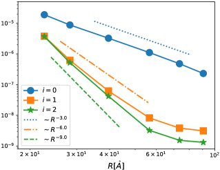
(a) Vacancy

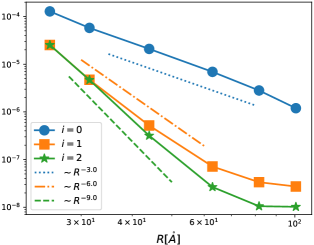
(b) Di-vacancy

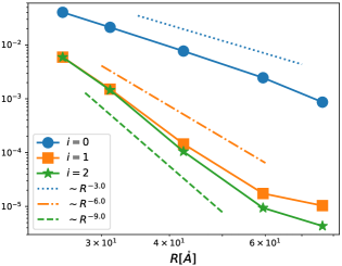
(c) Interstitial

Figure 4.4. Convergence of energy error $\big{|}\mathcal{E}(\bar{u})-\mathcal{E}(\bar{u}_{b_{i}})\big{|}$ for $i=0,1,2$ against domain size $R$ for vacancy, di-vacancy and interstitial.

5. Conclusion

In this paper, we design a novel family of numerical schemes exploiting the multipole expansions to accelerate the simulation of crystalline defect. In particular, the slow convergence rates of standard cell approximations for defect equilibration could be systematically improved by considering a novel moment iteration with a rigorously justified approximation. The proposed numerical schemes employ the approximate evaluation of multipole tensors, which are of important and ongoing interest in defect physics. To fulfill the efficient implementation, a continuous version of multipole expansion with continuous Green’s functions is also considered. Several prototypical numerical examples of point defects are presented to test the convergence for both geometry error and energy error. The numerical results show that our proposed numerical scheme can achieve the accelerated convergence rates in terms of computational cell size with the systematically improved boundary conditions.

Our presentation here is restricted to simple lattices and point defects. Generalisations do require additional technical difficulties to be overcome, but there appears to be no fundamental limitation to extend the method and the results to multi-lattices and a range of other defects in some form. To conclude, we briefly discuss some of these possibilities and limitations.

• Screw dislocations: We think that the extension of proposed numerical schemes from point defects to screw dislocations seems relatively straightforward. The substantial technical details are required and will be pursued separately. For example, how to solve the corresponding PDEs induced by the elastic-field with a high accuracy in the exterior domain, and how to couple the proposed moment iteration with the solutions of those PDEs. We refer to the recent work [2] for a simplified setting in this direction.

• Edge and mixed dislocations: Edge and mixed dislocations are technically more challenging but are practically more interesting compared with screw dislocations. They create a mismatch that affects the two-dimensional reference lattice, where a non-trivial transformation $u_{0}=u_{\rm CLE}\circ\xi^{-1}$ (cf. [12]) should be included to address this issue. The rigorous theory for edge and mixed dislocations is still lacking due to a substantial amount of additional technicality is required. For example, how to choose $\xi$, and what is the effect of such transformations have on those PDEs. See [3, Section 4] for a detailed discussion. Once the theory is established, it would be the place where the proposed numerical schemes reveal its most advantage and power and we believe that the idea of the current research should lead to the efficient and robust numerical schemes for those problems with fruitful practical interests.

• Multicale coupling methods: Several multiscale coupling methods (e.g., the atomistic-to-continuum (A/C) coupling [20, 32] or quantum mechanics/molecular mechanics (QM/MM) coupling [8, 33]) have been proposed to accelerate crystal defect computations in the last two decades. Our framework can provide a comprehensive analytical substructure for these methods to assess their relative accuracy and efficiency. In particular, it supplies a machinery for the optimisation of the non-trivial set of approximation parameters in multiscale schemes. The so-called truncation error would be improved such that a better balance between accuracy and efficiency might be achieved, which makes it possible for accurate large-scale atomistic simulations for crystalline defects.

Both the theoretical and practical aspects discussed above will be investigated in future work.

6. Proofs and extensions

After establishing the main numerical schemes in Section 3 and demonstrating their practical utilities in Section 4, we now provide the proofs and extensions that are helpful to understand the primary ideas of this paper in this section.

6.1. Proof of Theorem 3.2

Our goal is now to analyze the moment error $\big{\lvert}\mathcal{I}_{i,R}[\bar{v}_{b}]-\mathcal{I}_{i}[\bar{v}]\big{\rvert}$ for $i=1,\ldots,p$ in terms of the domain size $R$ for the purpose of estimating the unspecified errors $\big{\lvert}b^{(i,\cdot)}-b_{\rm exact}^{(i,\cdot)}\big{\rvert}$ shown in Lemma 3.1.

Proof.

We first split the moment error into two parts:

(6.29) $$\big{\lvert}\mathcal{I}_{i,R}[\bar{v}_{b}]-\mathcal{I}_{i}[\bar{v}]\big{\rvert}\leq\big{\lvert}\mathcal{I}_{i,R}[\bar{v}]-\mathcal{I}_{i}[\bar{v}]\big{\rvert}+\big{\lvert}\mathcal{I}_{i,R}[\bar{v}_{b}]-\mathcal{I}_{i,R}[\bar{v}]\big{\rvert}=:I_{1}+I_{2}.$$

To estimate $I_{1}$, after a straightforward manipulation, we can obtain

$$\big{\lvert}\mathcal{I}_{i,R}[\bar{v}]-\mathcal{I}_{i}[\bar{v}]\big{\rvert} \lesssim\sum_{\lvert\ell\rvert>R/3}\lvert\ell\rvert^{-d-p-1+i}\log^{p}(\lvert\ell\rvert)$$

(6.30) $$\lesssim R^{i-p-1}\log^{p}(R),$$

where the last inequality follows from the estimate in [3, Lemma 7.1].

For the term $I_{2}$, note that both $\bar{u}$ and $\bar{u}_{b}$ solve the discrete force equilibrium equations for $\lvert\ell\rvert<2R/3$ (actually $\lvert\ell\rvert<R-R_{0}$ is already necessary), hence we have

$$H[\bar{v}_{b}](\ell)-H[\bar{v}](\ell)=\int_{0}^{1}(1-t){\rm Div}\big{(} \nabla^{3}V(tD\bar{u}_{b})[D\bar{u}_{b},D\bar{u}_{b}]$$

(6.31) $$-\nabla^{3}V(tD\bar{u})[D\bar{u},D\bar{u}]\big{)}\,{\textrm{d}}t.$$

Before inserting the above term into the moment sum (2.3), we first estimate the stress difference in (6.1). Note that for any bounded Lipschitz function $f$ and any sub-multiplicative norm and product:

$$\big{\lvert}f(z)\cdot z\cdot z-f(x)\cdot x\cdot x\big{\rvert}\lesssim\lvert z-x\rvert(\lvert x\rvert+\lvert z-x\rvert)(1+\lvert x\rvert+\lvert z-x\rvert).$$

Hence, the stress difference in (6.1) can be further estimated by

$$\big{\lvert}\nabla^{3}V(tD\bar{u}_{b})[D\bar{u}_{b},D\bar{u}_{b}]-\nabla^{3}V(tD\bar{u})[D\bar{u},D\bar{u}]\big{\rvert}$$

$$\lesssim \lvert D\bar{v}_{b}-D\bar{v}\rvert\cdot\big{(}\lvert D\bar{u}\rvert+\lvert D\bar{v}_{b}-D\bar{v}\rvert\big{)}\cdot\big{(}1+\lvert D\bar{u}\rvert+\lvert D\bar{v}_{b}-D\bar{v}\rvert\big{)}$$

$$\lesssim \lvert D\bar{v}_{b}-D\bar{v}\rvert\cdot\big{(}\lvert\ell\rvert^{-d}+\lvert D\bar{v}_{b}-D\bar{v}\rvert\big{)},$$

where the last inequality follows from the decay estimate of the equilibrium for point defects [12, Theorem 1]. Inserting that into the moment sum after partially summing, we obtain

$$\big{\lvert}\mathcal{I}_{i,R}[\bar{v}_{b}]-\mathcal{I}_{i,R}[\bar{v}]\big{\rvert}$$

$$\lesssim ~{}\int_{0}^{1}(1-t)\sum_{\ell\in\Lambda\cap B_{2R/3}({\bf 0})}\lvert\ell\rvert^{i-1}\cdot\big{\lvert}\nabla^{3}V(tD\bar{u}_{b})[D\bar{u}_{b},D\bar{u}_{b}]-\nabla^{3}V(tD\bar{u})[D\bar{u},D\bar{u}]\big{\rvert}\,{\textrm{d}}t$$

$$\lesssim ~{}\sum_{\ell\in\Lambda\cap B_{2R/3}({\bf 0})}\lvert\ell\rvert^{i-1}\cdot\lvert D\bar{v}_{b,R}-D\bar{v}\rvert\cdot\big{(}\lvert\ell\rvert^{-d}+\lvert D\bar{v}_{b,R}-D\bar{v}\rvert\big{)}$$

(6.32) $$\lesssim ~{}\lVert D\bar{v}_{b}-D\bar{v}\rVert_{\ell^{2}}\cdot\Bigg{(}R^{i-1}\lVert D\bar{v}_{b}-D\bar{v}\rVert_{\ell^{2}}+\Bigg{(}\sum_{\ell\in\Lambda\cap B_{2R/3}({\bf 0})}\lvert\ell\rvert^{i-2-2d}\Bigg{)}^{1/2}\Bigg{)},$$

where the last term can be further estimated by

$$\Bigg{(}\sum_{\ell\in\Lambda\cap B_{2R/3}({\bf 0})}\lvert\ell\rvert^{2i-2-2d}\Bigg{)}^{1/2}\lesssim\alpha_{i}(R):=\begin{cases}1&~{}i<1+d/2\\ \log(R)&~{}i=1+d/2\\ R^{i-1-d/2}&~{}i>1+d/2\end{cases}.$$

Combing (6.29), (6.1) with (6.1), we obtain

(6.33) $$\big{\lvert}\mathcal{I}_{i,R}[\bar{v}_{b}]-\mathcal{I}_{i}[\bar{v}]\big{\rvert}\lesssim R^{i-p-1}\log^{p}(R)+R^{i-1}\big{\lVert}D\bar{v}_{b}-D\bar{v}\rVert_{\ell^{2}}^{2}+\alpha_{i}(R)\lVert D\bar{v}_{b}-D\bar{v}\rVert_{\ell^{2}},$$

which yields the stated result. ∎

6.2. The relation between moments, discrete and continuous coefficients

In this section, we derive the concrete relationship between moments and the coefficients for both discrete and continuous expansions (cf. (2.5) and (4.23)). As discussed in Remark 3.2, we mainly focus on the case of $d=3$ and $p=3$. Hence, we need to utilize the first three terms in the multipole expansions. More precisely, from Theorem 2.1 and Lemma 4.1, the decomposition of equilibrium $\bar{u}$ can be expressed in terms of both discrete and continuous terms

$$\bar{u} =~{}\sum_{k=1}^{3}b^{(1,k)}:D_{\mathcal{S}}(\mathcal{G})_{\cdot k}+\sum_{k=1}^{3}b^{(2,k)}:D^{2}_{\mathcal{S}}(\mathcal{G})_{\cdot k}+\sum_{k=1}^{3}b^{(3,k)}:D^{3}_{\mathcal{S}}(\mathcal{G})_{\cdot k}+O(\lvert\ell\rvert^{-5}),$$

$$=~{}\Bigg{(}\sum_{k=1}^{3}a^{(1,0,k)}:\nabla(G_{0})_{\cdot k}+\sum_{k=1}^{3}a^{(1,1,k)}:\nabla(G_{1})_{\cdot k}\Bigg{)}+\sum_{k=1}^{3}a^{(2,0,k)}:\nabla^{2}(G_{0})_{\cdot k}$$

$$\quad+\sum_{k=1}^{3}a^{(3,0,k)}:\nabla^{3}(G_{0})_{\cdot k}+O(\lvert\ell\rvert^{-5})$$

(6.34) $$=:~{}u_{1}+u_{2}+u_{3}+O(\lvert\ell\rvert^{-5}).$$

The relation between the continuous coefficients $a^{(i,n,k)}$ and the discrete coefficients $b^{(i,k)}$

In order to derive the identities shown in (4.1), we first Taylor expand the discrete difference stencil as well as its higher discrete difference at site $\ell$, for any $\rho,\sigma,\tau\in\mathcal{R}$,

$$D_{\rho}\mathcal{G} =\nabla_{\rho}G_{0}+\nabla_{\rho}G_{1}+\frac{1}{2}\nabla^{2}_{\rho\rho}G_{0}+\frac{1}{6}\nabla^{3}_{\rho\rho\rho}G_{0}+{\rm h.o.t.},$$

$$D^{2}_{\rho\sigma}\mathcal{G} =\nabla^{2}_{\rho\sigma}G_{0}+\frac{1}{2}\nabla^{3}_{\rho\sigma\sigma}G_{0}+\frac{1}{2}\nabla^{3}_{\rho\rho\sigma}G_{0}+{\rm h.o.t.},$$

$$D^{3}_{\rho\sigma\tau}\mathcal{G} =\nabla^{3}_{\rho\sigma\tau}G_{0}+{\rm h.o.t.}.$$

According to $u_{1}$ in (6.2), by matching the first-order terms and applying the above identities, we can obtain

$$\sum_{j,k=1}^{3}\Big{(}(a^{(1,0,k)})_{\cdot j}\cdot\partial_{j}(G_{0})_{\cdot k}+(a^{(1,1,k)})_{\cdot j}\cdot\partial_{j}(G_{1})_{\cdot k}\Big{)}$$

$$=~{} \sum_{k=1}^{3}\sum_{\rho\in\mathcal{R}}(b^{(1,k)})_{\rho}\cdot D_{\rho}\mathcal{G}_{\cdot k}$$

$$=~{} \sum_{j,k=1}^{3}\sum_{\rho\in\mathcal{R}}\Big{(}(b^{(1,k)})_{\rho}\cdot\partial_{j}(G_{0})_{\cdot k}\cdot\rho_{j}+(b^{(1,k)})_{\rho}\cdot\partial_{j}(G_{1})_{\cdot k}\cdot\rho_{j}\Big{)}.$$

Hence, for each $j,k=1,2,3$,

(6.35) $$(a^{(1,0,k)})_{\cdot j}=(a^{(1,1,k)})_{\cdot j}=\sum_{\rho\in\mathcal{R}}(b^{(1,k)})_{\rho}\cdot\rho_{j}.$$

To get the second-order coefficients ($i=2$), it is necessary to consider the term $u_{2}$ as well as the square term in $u_{1}$, that is,

$$\sum_{j,m,k=1}^{3}(a^{(2,0,k)})_{\cdot jm}\cdot\partial^{2}_{jm}(G_{0})_{\cdot k}= ~{}\sum_{k=1}^{3}\sum_{\rho,\sigma\in\mathcal{R}}(b^{(2,k)})_{\rho\sigma}\cdot D^{2}_{\rho\sigma}\mathcal{G}_{\cdot k}+\sum_{k=1}^{3}\sum_{\rho\in\mathcal{R}}(b^{(1,k)})_{\rho}\cdot\Big{(}\frac{1}{2}\nabla^{2}_{\rho\rho}G_{0}\Big{)}_{\cdot k}$$

$$= ~{}\sum_{j,m,k=1}^{3}\sum_{\rho,\sigma\in\mathcal{R}}(b^{(2,k)})_{\rho\sigma}\cdot\partial^{2}_{jm}(G_{0})_{\cdot k}\cdot\rho_{j}\sigma_{m}$$

$$+\frac{1}{2}\sum_{j,m,k=1}^{3}\sum_{\rho\in\mathcal{R}}(b^{(1,k)})_{\rho}\cdot\partial^{2}_{jm}(G_{0})_{\cdot k}\cdot\rho_{j}\rho_{m}.$$

Hence, for each $j,m,k=1,2,3$, we have

$$(a^{(2,0,k)})_{\cdot jm}= \sum_{\rho,\sigma\in\mathcal{R}}(b^{(2,k)})_{\rho\sigma}\cdot\rho_{j}\sigma_{m}+\frac{1}{2}\sum_{\rho\in\mathcal{R}}(b^{(1,k)})_{\rho}\cdot\rho_{j}\rho_{m}$$

(6.36) $$= \sum_{\rho,\sigma\in\mathcal{R}}(b^{(2,k)})_{\rho\sigma}\cdot\rho_{j}\sigma_{m}+\frac{1}{2}\sum_{\rho\in\mathcal{R}}(a^{(1,0,k)})_{\cdot j}\cdot\rho_{m}.$$

Analogously, after a tedious calculation, we obtain the following identity

$$\sum_{j,m,n,k=1}^{3}(a^{(3,0,k)})_{\cdot jmn}\cdot\partial^{3}_{jmn}(G_{0})_{\cdot k}$$

$$= ~{}\sum_{k=1}^{3}\sum_{\rho,\sigma,\tau\in\mathcal{R}}(b^{(3,k)})_{\rho\sigma\tau}\cdot D^{3}_{\rho\sigma\tau}\mathcal{G}_{\cdot k}+\sum_{k=1}^{3}\sum_{\rho,\sigma\mathcal{R}}(b^{(2,k)})_{\rho\sigma}\cdot\Big{(}\frac{1}{2}\nabla^{3}_{\rho\sigma\sigma}G_{0}+\frac{1}{2}\nabla^{3}_{\rho\rho\sigma}G_{0}\Big{)}_{\cdot k}$$

$$+\sum_{k=1}^{3}\sum_{\rho\in\mathcal{R}}(b^{(1,k)})_{\rho}\cdot\Big{(}\frac{1}{6}\nabla^{3}_{\rho\rho\rho}G_{0}\Big{)}_{\cdot k}$$

$$= \sum_{j,m,n,k=1}^{3}\sum_{\rho,\sigma,\tau\in\mathcal{R}}(b^{(3,k)})_{\rho\sigma\tau}\cdot\partial^{3}_{jmn}(G_{0})_{\cdot k}\cdot\rho_{j}\sigma_{m}\tau_{n}$$

$$+\frac{1}{2}\sum_{j,m,n,k=1}^{3}\sum_{\rho,\sigma\in\mathcal{R}}(b^{(2,k)})_{\rho\sigma}\cdot\partial^{3}_{jmn}(G_{0})_{\cdot k}\cdot(\rho_{j}\sigma_{m}\sigma_{n}+\rho_{j}\rho_{m}\sigma_{n})$$

$$+\frac{1}{6}\sum_{j,m,n,k=1}^{3}\sum_{\rho\in\mathcal{R}}(b^{(1,k)})_{\rho}\cdot\partial^{3}_{jmn}(G_{0})_{\cdot k}\cdot\rho_{j}\rho_{m}\rho_{n}.$$

Therefore, if we denote $a^{(3,0,k)}$ as a collection of $(a^{(3,0,k)})_{\cdot jmn}$ for all $j,m,n=1,2,3$, then for each $k=1,2,3$, we can obtain

$$a^{(3,0,k)}= \sum_{\rho,\sigma,\tau\in\mathcal{R}}(b^{(3,k)})_{\rho\sigma\tau}\cdot\rho\otimes\sigma\otimes\tau+\sum_{\rho,\sigma\in\mathcal{R}}(b^{(2,k)})_{\rho\sigma}\cdot\rho\odot\sigma\odot\sigma$$

(6.37) $$+\frac{1}{6}\sum_{\rho\in\mathcal{R}}(b^{(1,k)})_{\rho}\cdot\rho\otimes\rho\otimes\rho.$$

Taking into account (6.35), (6.2) with (6.2), we acquire the relationship between $a^{(i,n,k)}$ and $b^{(i,k)}$ (cf. (4.1)).

The relation between moments $\mathcal{I}_{i}[\bar{u}]$ and discrete coefficients $b^{(i,k)}$

Next, we give a concrete formulation of (2.8). From the definition of force moments, for $i=1,2,3$, we have

(6.38) $$\mathcal{I}_{i}[\bar{u}]=\sum_{\ell\in\Lambda}H[\bar{u}](\ell)\otimes\ell^{\otimes i}.$$

The relation between moments and discrete coefficients is derived based on (6.38). As a matter of fact, recalling the decomposition (6.2) and the fact that $H[\mathcal{G}_{\cdot k}](\ell)=\delta_{0,\ell}e_{k}$, we can obtain

$$H[u_{1}]= H\Bigg{[}\sum_{k=1}^{3}b^{(1,k)}:D_{\mathcal{S}}(\mathcal{G})_{\cdot k}\Bigg{]}=\sum_{k=1}^{3}\sum_{\rho\in\mathcal{R}}b^{(1,k)}_{\rho}\cdot D_{\rho}\delta_{0}e_{k},$$

(6.39) $$H[u_{2}]= H\Bigg{[}\sum_{k=1}^{3}b^{(2,k)}:D^{2}_{\mathcal{S}}(\mathcal{G})_{\cdot k}\Bigg{]}=\sum_{k=1}^{3}\sum_{\rho,\sigma\in\mathcal{R}}(b^{(2,k)})_{\rho\sigma}\cdot D^{2}_{\rho\sigma}\delta_{0}e_{k},$$

$$H[u_{3}]= H\Bigg{[}\sum_{k=1}^{3}b^{(3,k)}:D^{3}_{\mathcal{S}}(\mathcal{G})_{\cdot k}\Bigg{]}=\sum_{k=1}^{3}\sum_{\rho,\sigma,\tau\in\mathcal{R}}(b^{(2,k)})_{\rho\sigma\tau}\cdot D^{3}_{\rho\sigma\tau}\delta_{0}e_{k}.$$

Hence, combining (6.38) with (6.2), one can acquire that

$$\mathcal{I}_{1}[\bar{u}] =\sum_{k=1}^{3}\sum_{\rho\in\mathcal{R}}\sum_{\ell\in\Lambda}(b^{(1,k)})_{\rho}\cdot D_{\rho}\delta_{0}e_{k}\otimes\ell$$

$$=-\sum_{k=1}^{3}\sum_{\rho\in\mathcal{R}}(b^{(1,k)})_{\rho}\cdot e_{k}\otimes\rho$$

(6.40) $$=-\sum_{j,k=1}^{3}\sum_{\rho\in\mathcal{R}}(b^{(1,k)})_{\rho}\cdot\rho_{j}\cdot e_{k}\otimes e_{j},$$

which yields the relation between the first order coefficient $b^{(1,\cdot)}$ and dipole moment $\mathcal{I}_{1}[\bar{u}]$.

As for the tripole moment $\mathcal{I}_{2}[\bar{u}]$, similarly we have

$$\mathcal{I}_{2}[\bar{u}]= \sum_{k=1}^{3}\sum_{\rho\in\mathcal{R}}\sum_{\ell\in\Lambda}(b^{(1,k)})_{\rho}\cdot D_{\rho}\delta_{0}e_{k}\otimes\ell\otimes\ell+\sum_{k=1}^{3}\sum_{\rho,\sigma\in\mathcal{R}}\sum_{\ell\in\Lambda}(b^{(2,k)})_{\rho\sigma}\cdot D^{2}_{\rho\sigma}\delta_{0}e_{k}\otimes\ell\otimes\ell$$

$$= \sum_{k=1}^{3}\sum_{\rho\in\mathcal{R}}(b^{(1,k)})_{\rho}e_{k}\otimes\rho\otimes\rho+2\sum_{k=1}^{3}\sum_{\rho,\sigma\in\mathcal{R}}(b^{(2,k)})_{\rho\sigma}\cdot e_{k}\otimes\rho\otimes\sigma$$

(6.41) $$= \sum_{j,m,k=1}^{3}\sum_{\rho\in\mathcal{R}}(b^{(1,k)})_{\rho}\cdot\rho_{j}\rho_{m}e_{k}\otimes e_{j}\otimes e_{m}+2\sum_{j,m,k=1}^{3}\sum_{\rho,\sigma\in\mathcal{R}}(b^{(2,k)})_{\rho\sigma}\cdot\rho_{j}\sigma_{m}\cdot e_{k}\otimes e_{j}\otimes e_{m}.$$

For the quadrupole moment $\mathcal{I}_{3}[\bar{u}]$, with a tedious calculation, we can obtain

$$\mathcal{I}_{3}[\bar{u}]= \sum_{k=1}^{3}\sum_{\rho\in\mathcal{R}}\sum_{\ell\in\Lambda}(b^{(1,k)})_{\rho}\cdot D_{\rho}\delta_{0}e_{k}\otimes\ell\otimes\ell\otimes\ell+\sum_{k=1}^{3}\sum_{\rho,\sigma\in\mathcal{R}}\sum_{\ell\in\mathcal{R}}(b^{(2,k)})_{\rho\sigma}\cdot D^{2}_{\rho\sigma}\delta_{0}e_{k}\otimes\ell\otimes\ell\otimes\ell$$

$$+\sum_{k=1}^{3}\sum_{\rho,\sigma,\tau\in\mathcal{R}}\sum_{\ell\in\Lambda}(b^{(3,k)})_{\rho\sigma\tau}\cdot D^{3}_{\rho\sigma\tau}\delta_{0}e_{k}\otimes\ell\otimes\ell\otimes\ell$$

$$= \sum_{k=1}^{3}\sum_{\rho\in\mathcal{R}}\sum_{\ell\in\Lambda}(b^{(1,k)})_{\rho}\cdot e_{k}\otimes D_{-\rho}\Big{(}\ell\otimes\ell\otimes\ell\Big{)}$$

$$+\sum_{k=1}^{3}\sum_{\rho,\sigma\in\mathcal{R}}\sum_{\ell\in\Lambda}(b^{(2,k)})_{\rho\sigma}\cdot e_{k}\otimes D_{-\rho}D_{-\sigma}\Big{(}\ell\otimes\ell\otimes\ell\Big{)}$$

$$+\sum_{k=1}^{3}\sum_{\rho,\sigma,\tau\in\mathcal{R}}\sum_{\ell\in\Lambda}(b^{(3,k)})_{\rho\sigma\tau}\cdot e_{k}\otimes D_{-\rho}D_{-\sigma}D_{-\tau}\Big{(}\ell\otimes\ell\otimes\ell\Big{)}$$

$$= -\sum_{k=1}^{3}\sum_{\rho\in\mathcal{R}}(b^{(1,k)})_{\rho}\cdot e_{k}\otimes\rho\otimes\rho\otimes\rho-6\sum_{k=1}^{3}\sum_{\rho,\sigma\in\mathcal{R}}(b^{(2,k)})_{\rho\sigma}\cdot e_{k}\otimes\rho\odot\sigma\odot\sigma$$

(6.42) $$-6\sum_{k=1}^{3}\sum_{\rho,\sigma,\tau\in\mathcal{R}}(b^{(3,k)})_{\rho\sigma\tau}\cdot e_{k}\otimes\rho\odot\sigma\odot\tau.$$

Hence, we yield the results in [3, Lemma 5.6] or (2.8).

The relation between the moments $I_{i}[\bar{u}]$ and the continuous coefficients $a^{(i,n,k)}$

Combining the results presented above, we then derive the relation between the moments $I_{i}[\bar{u}]$ and the continuous coefficients $a^{(i,n,k)}$. More precisely, for the dipole moment, by inserting (6.35) and (6.2) into (6.2), we have

$$\mathcal{I}_{1}[\bar{u}]=-\sum_{j,k=1}^{3}\sum_{\rho\in\mathcal{R}}(b^{(1,k)})_{\rho}\cdot\rho_{j}\cdot e_{k}\otimes e_{j}=-a^{(1,0,\cdot)}=-a^{(1,1,\cdot)}.$$

Similarly, taking into account (6.2) with (6.2), we get

$$\mathcal{I}_{2}[\bar{u}]= \sum_{j,m,k=1}^{3}\sum_{\rho\in\mathcal{R}}(b^{(1,k)})_{\rho}\cdot\rho_{j}\rho_{m}\cdot e_{k}\otimes e_{j}\otimes e_{m}$$

$$+2\sum_{j,m,k=1}^{3}\sum_{\rho,\sigma\in\mathcal{R}}(b^{(2,k)})_{\rho\sigma}\cdot\rho_{j}\sigma_{m}\cdot e_{k}\otimes e_{j}\otimes e_{m}$$

$$= \sum_{j,m,k=1}^{3}\Big{(}\sum_{\rho\in\mathcal{R}}(a^{(1,0,k)})_{\cdot j}\cdot\rho_{m}\Big{)}e_{k}\otimes e_{j}\otimes e_{m}$$

$$+\sum_{j,m,k=1}^{3}\Big{(}2(a^{(2,0,k)})_{\cdot jm}-\sum_{\rho\in\mathcal{R}}(a^{(1,0,k)})_{\cdot j}\cdot\rho_{m}\Big{)}e_{k}\otimes e_{j}\otimes e_{m}$$

$$= ~{}2a^{(2,0,\cdot)}.$$

As for the third order term (quadrupole moment), adding (6.2) into (6.2) and after a direct algebraic manipulation, one can acquire that

(6.43) $$\mathcal{I}_{3}[\bar{u}]=-6a^{(3,0,\cdot)}.$$

Hence, we obtain the practical formulation of continuous coefficients for $i=1,2,3$ via force moments

$$a^{(1,0,\cdot)} =-\mathcal{I}_{1}[\bar{u}],\quad a^{(1,1,\cdot)}=-\mathcal{I}_{1}[\bar{u}],$$

(6.44) $$a^{(2,0,\cdot)} =\frac{1}{2}\mathcal{I}_{2}[\bar{u}],\quad a^{(3,0,\cdot)}=-\frac{1}{6}\mathcal{I}_{3}[\bar{u}],$$

which are applied directly in the numerical tests (cf. Algorithm 4.2).

6.3. The computation of continuous Green’s functions

In this section, we briefly discuss the implementation of the continuous Green’s functions employed in the practical computation of higher order correctors (cf. Algorithm 4.2). The resulting expressions provide us with the ability to directly deduce regularity, decay, and even homogeneity [3]. More importantly, the representation is promising for computational uses as only a finite surface integral in Fourier space is required for its evaluation.

The continuous Green’s functions and their higher order correction can be expressed by applying the Morrey formula (cf. [3, Section 6.4]), that is, for $n\geq 1$ and $\ell\neq 0$

(6.45) $$G_{n}(\ell)=(-\Delta)^{P}\frac{c_{\rm vol}}{(2\pi)^{d}}\int_{\mathbb{S}^{d-1}}\mathcal{A}_{2n-2}(\sigma)J_{-1-h}(\ell\cdot\sigma)\,{\textrm{d}}\sigma,$$

where $P=\lceil\frac{d+2n-1}{2}\rceil$, $\Delta$ is the Laplacian, and

$$J_{t}(w) =t!(-iw)^{-t-1}, \text{ for }t\geq 0$$

$$J_{t}(w) =\frac{1}{(-t-1)!}(iw)^{-t-1}\Big{(}-\log(-iw)+\sum_{j=1}^{-t-1}j^{-1}\Big{)}, \text{ for }t<0,$$

where $J_{t}^{\prime}(w)=iJ_{t+1}(w)$ is satisfied. We only consider $d=3$ throughout this paper and the results for $d=2$ could be obtained similarly. In particular, $G_{0}$ reads

(6.46) $$G_{0}(\ell)=(-\Delta)\frac{c_{\rm vol}}{(2\pi)^{3}}\int_{\mathbb{S}^{2}}\mathcal{A}_{-2}(\sigma)J_{-2}(\ell\cdot\sigma)\,{\textrm{d}}\sigma.$$

Note that $\mathcal{A}_{-2}=\widehat{H}_{2}^{-1}$ where $\widehat{H}_{2n}^{-1}$, the inverse of the discrete lattice operator Fourier multiplier [5, 16], is explicitly defined in [3, Section 6.2]. For real $w$ we have the identity

$${\rm Re}J_{-2}(w)=(-iw)i{\rm Arg}(-iw)=-\pi/2\lvert w\rvert.$$

Hence, one can further write (6.46) as

(6.47) $$G_{0}(\ell)=\frac{c_{\rm vol}}{16\pi^{2}}\Delta\int_{\mathbb{S}^{2}}\mathcal{A}_{-2}(\sigma)\lvert\ell\cdot\sigma\rvert\,{\textrm{d}}\sigma.$$

As discussed in [3, Section 6], we already know that the integral defines a $C^{\infty}$ function, one can easily evaluate the derivatives in the distributional sense, and therefore we obtain

(6.48) $$G_{0}(\ell)=\frac{c_{\rm vol}}{8\pi^{2}}\int_{\mathbb{S}^{2}\cap\{\sigma\cdot x=0\}}\mathcal{A}_{-2}(\sigma)\,{\textrm{d}}\sigma,$$

which yields a rigorous derivation of Barnett’s formula [1].

Applying (6.45) as well as the similar calculation as that on $G_{0}(\ell)$, the first order correction $G_{1}(\ell)$ can be rewritten as

$$G_{1}(\ell) =(\Delta)^{2}\frac{c_{\rm vol}}{(2\pi)^{3}}\int_{\mathbb{S}^{2}}\mathcal{A}_{0}(\sigma)J_{-2}(\ell\cdot\sigma)\,{\textrm{d}}\sigma$$

(6.49) $$=\frac{c_{\rm vol}}{8\pi^{2}}\Delta\int_{\mathbb{S}^{2}\cap\{\sigma\cdot x=0\}}\mathcal{A}_{0}(\sigma)\,{\textrm{d}}\sigma,$$

where $\mathcal{A}_{0}:=-\widehat{H}_{2}^{-1}\widehat{H}_{4}\widehat{H}_{2}^{-1}$.

In practical implementation, we make full use of (6.48) and (6.3) to obtain the continuous Green’s function $G_{0}$ and its first order correction $G_{1}$. Furthermore, the higher order derivatives of $G_{0}$ up to the third order are required as well during the computations, namely $\nabla^{j}G_{0}$, $j=1,2,3$, which are obtained using the technique of automatic differentiation [25].

6.4. Alternative approach

As mentioned in Remark 3.1, the scheme (3.13) cannot be implemented in practice since the energy difference functional cannot be assessed for a displacement with infinite range. To fulfill the fast and accurate evaluation of the far-field predictors in the main context, we propose a novel moment iteration by engaging in the approximate evaluation of the multipole tensors.

In this section, we consider an alternative approach that provides suitable controlled approximation to $\mathcal{E}$, somewhat analogous to the variational crimes in the field of classical numerical analysis [18, 24].

To proceed, we leave the discrete coefficients $b_{\rm exact}$ introduced in Section 3.1 as free parameters which are optimized as part of the core minimization as outlined in [3]. This can however not be done directly as the energy depends on these $b$ everywhere and one would need to evaluate the energy on the entire (infinite) $\Lambda$. Therefore we now want to introduce an alternative approximation by truncating the energy functional $\mathcal{E}$. Recall the definition (2.1), it can be rewritten as

$$\mathcal{E}(u)=\sum_{\ell\in\Lambda}\Big{[}V\big{(}Du(\ell)\big{)}-V({\bf 0})-\big{(}\nabla V({\bf 0})+{\bm{g}}\big{)}\cdot Du(\ell)\Big{]},$$

where $\bm{g}$ comes from the inhomogeneous defect part, and the following analysis is independent of its concrete formulation. Given the radius of finite domain $R$ and $r\geq 3R$, let $\eta_{r}:\Lambda\rightarrow\mathbb{R}$ be a smooth cut-off function introduced in Section 3.2. We then define the truncated energy functional

$$\mathcal{E}_{r}(u):=\mathcal{E}(u)\cdot\eta_{r}:=\sum_{\ell\in\Lambda}\Big{[}V\big{(}Du(\ell)\big{)}-V({\bf 0})-\big{(}\nabla V({\bf 0})+{\bm{g}}\big{)}\cdot Du(\ell)\Big{]}\cdot\eta_{r}(\ell).$$

Our purpose is to minimize this energy functional over the exact admissible corrector space

$$\mathcal{U}^{(3)}_{R}:=\big{\{}v:\Lambda\to\mathbb{R}^{N}\,|\, \,\,v=\sum_{i=1}^{3}\sum_{k=1}^{N}b^{(i,k)}_{\rm exact}:D^{i}_{\mathcal{S}}\mathcal{G}_{k}+w,$$

$$\text{for any $w$ with ${\rm supp}~{}w\subset\Lambda\cap B_{R}$ and any $b^{(i,k)}_{\rm exact}$}\big{\}},$$

where we fix $p=3$ in this section.

Following the notations in Theorem 3.1, let $\bar{u}_{3,R}$ and $\bar{u}_{3,R,r}$ be the minimizers of $\mathcal{E}$ and $\mathcal{E}_{r}$ over $\mathcal{U}^{(3)}_{R}$ respectively. We now want to show that for sufficiently large $r$, $\bar{u}_{3,R}$ is an approximate solution to $\mathcal{E}_{r}$ with a consistency estimate as well as a suitable stable condition is satisfied, so that the inverse function theorrm (cf. Lemma 6.1) yields a solution $\bar{u}_{3,R,r}$ that has the corresponding convergence rates in terms of $r$.

We first state an important property of functions belonging to $\mathcal{U}^{(3)}_{R}$, which essentially shows the norm equivalence between the corrector and its reminder term up to a constant that depends on the discrete coefficients $b^{(i,\cdot)}_{\rm exact}$. For $v\in\mathcal{U}^{(3)}_{R}$, after a straightforward manipulation, we have the following estimate

(6.50) $$\lVert Dv\rVert_{\ell^{2}}\lesssim\lVert Dw\rVert_{\ell^{2}}+\sum_{i=1}^{3}\sum_{k=1}^{N}\lvert b^{(i,k)}_{\rm exact}\rvert\lesssim\lVert Dv\rVert_{\ell^{2}}.$$

Before we give the main estiamte in this section, we first review a quantitative version of the inverse function theorem, adapted from [20, Lemma B.1].

Lemma 6.1.

Let $X,Y$ be Hilbert spaces, $w\in X$, $F\in C^{2}(B^{X}_{R}(w);Y)$ with Lipschitz continuous Hessian, $\|\delta^{2}F(x)-\delta^{2}F(y)\|_{L(X,Y)}\leq M\|x-y\|_{X}$ for any $x,y\in B^{X}_{R}(w)$. Furthermore, suppose that there exist constants $\mu,r>0$ such that

$$\langle\delta^{2}F(w)v,v\rangle\geq\mu\|v\|^{2}_{X},\quad\|\delta F(w)\|_{Y}\leq r,\quad\textrm{and}~{}\frac{2Mr}{\mu^{2}}<1,$$

then there exists a locally unique $\bar{w}\in B^{X}_{R}(w)$ such that $\delta F(\bar{w})=0,\|w-\bar{w}\|_{X}\leq\frac{2r}{\mu}$ and

$$\langle\delta^{2}F(\bar{w})v,v\rangle\geq\big{(}1-\frac{2Mr}{\mu^{2}}\big{)}\mu\|v\|^{2}_{X}.$$

Stability:

To utilize Lemma 6.1, we first check the stability of $\bar{u}_{3,R}$. For any $v\in\mathcal{U}^{(3)}_{R}$, we can obtain

$$~{}\big{\lvert}\delta^{2}\mathcal{E}_{r}(\bar{u}_{3,R})[v,v]-\delta^{2}\mathcal{E}(\bar{u}_{3,R})[v,v]\big{\rvert}$$

$$\leq ~{}\Big{\lvert}\sum_{\ell\in\Lambda}\nabla^{2}V\big{(}D\bar{u}_{3,R}(\ell)\big{)}[Dv,Dv]\cdot\big{(}1-\eta_{r}(\ell)\big{)}\Big{\rvert}$$

$$\lesssim ~{}\sum_{i=1}^{3}\sum_{k=1}^{N}\lvert b^{(i,k)}\rvert\cdot\sum_{\ell\in\Lambda}\lvert\ell\rvert^{-6}\big{(}1-\eta_{r}(\ell)\big{)}$$

$$\lesssim ~{}\lVert Dv\rVert_{\ell^{2}}^{2}\cdot r^{-3},$$

where the last inequality follows from the estimate (6.50).

Hence, for sufficiently large $r$ and any $v\in\mathcal{U}_{R}$, we have

(6.51) $$\delta^{2}\mathcal{E}_{r}(\bar{u}_{3,R})[v,v]\geq c_{0}/2\cdot\lVert Dv\rVert_{\ell^{2}}^{2},$$

where $c_{0}>0$ is known as the stability constant of $\delta^{2}\mathcal{E}(\bar{u}_{3,R})$.

Consistency:

Next, we need to show that the first variation of the truncated energy functional evaluated on the approximate solution $\bar{u}_{3,R}$ is consistent. For any $v\in\mathcal{U}^{(3)}_{R}$, it follows that

$$\big{\lvert}\langle\delta\mathcal{E}_{r}(\bar{u}_{3,R}),v\rangle\big{\rvert} =\big{\lvert}\langle\delta\mathcal{E}_{r}(\bar{u}_{3,R})-\delta\mathcal{E}(\bar{u}_{3,R}),v\rangle\big{\rvert}$$

$$=\Big{\lvert}\sum_{\ell\in\Lambda}\Big{(}\nabla V\big{(}D\bar{u}_{3,R}(\ell)\big{)}-\nabla V({\bf 0})\Big{)}[Dv]\cdot\big{(}1-\eta_{r}(\ell)\big{)}\Big{\rvert}$$

$$=\Bigg{\lvert}\int_{0}^{1}\sum_{\ell\in\Lambda}\nabla^{2}V\big{(}tD\bar{u}_{3,R}(\ell)\big{)}[D\bar{u}_{3,R},Dv]\cdot\big{(}1-\eta_{r}(\ell)\big{)}\,{\textrm{d}}t\Bigg{\rvert}$$

$$\lesssim\sum_{i=1}^{3}\sum_{k=1}^{N}\lvert b^{(i,k)}\rvert\cdot\sum_{\ell\in\Lambda}\lvert\ell\rvert^{-6}\big{(}1-\eta_{r}(\ell)\big{)}$$

(6.52) $$\lesssim\lVert Dv\rVert_{\ell^{2}}\cdot r^{-3}.$$

Applying the inverse function theorem:

Combining (6.51) with (6.4) and applying Lemma 6.1, we can conclude that, for sufficiently large $r$, there exists a solution $\bar{u}_{3,R,r}\in\mathcal{U}^{(3)}_{R}$ satisfying

$$\lVert D\bar{u}_{3,R,r}-D\bar{u}_{3,R}\rVert_{\ell^{2}}\lesssim r^{-3}.$$

If we choose $r=CR^{3/2}$, then we have

$$\lVert D\bar{u}_{3,R,r}-D\bar{u}_{3,R}\rVert_{\ell^{2}}\lesssim R^{-9/2}.$$

Applying Theorem 3.1, we can obtain

$$\lVert D\bar{u}_{3,R,r}-D\bar{u}\rVert_{\ell^{2}}\lesssim R^{-9/2}\log(R),$$

which is the same estimate on the geometry error as that shown in Corollary 3.1.

It is worthwhile mentioning that the estimate on the energy error can be similarly obtained by employing the techniques in proving Theorem 3.1. We also note that different from the moment iteration, this alternative approach is independent of the choice of $p$. More precisely, if one just wants $p=1$, then we will get $R^{-5/2}$ estimate in (6.4) leading to the fact that $r=CR$ is already sufficient.

7. Numerical supplements

7.1. Decay of strains

The decay of correctors in strains, serving as a direct application of Theorem 2.1, is tested in this section. Figure 7.5 plots the decay of correctors in strains $|D\bar{u}_{b_{i}}(\ell)|$ with different orders of predictors constructed by Algorithm 4.2 for all crystalline defects considered in this work. Transparent dots denote the corresponding data points ($|\ell|,|D\bar{u}_{b_{i}}(\ell)|$) for $i=0,1,2$ and solid curves plot their envelops. The numerically observed improved decay for higher-order predictors is consistent with our theoretical results (Remark 3.2).

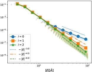
(a) Vacancy

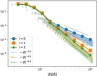
(b) Divacancy

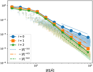
(c) Interstitial

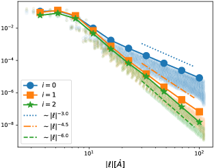
(d) Micro-crack-2

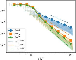
(e) Micro-crack-3

Figure 7.5. Decay of strains $|D\bar{u}_{b_{i}}(\ell)|$ for $i=0,1,2$ for all types of crystalline defect considered in this work.

7.2. Convergence for micro-cracks

In this part, we collect the numerical results for the two micro-cracks cases (i.e., micro-crack-2 and micro-crack-3 introduced in Section 2.1). Figure 7.6, Figure 7.7 and Figure 7.8 plot the convergence of moments ${\rm ME}_{ki}$ defined by (4.28), geometry error $\|D\bar{u}-D\bar{u}_{b_{i}}\|_{\ell^{2}}$ and energy error $\big{|}E(\bar{u})-E(\bar{u}_{b_{i}})\big{|}$ for $i=0,1,2$ in the cell problems with respect to the domain size $R$, respectively. These results are very similar as those shown in Section 4.3, which again confirm the prediction of the theory presented in the main context. Moreover, these results also indicate that our numerical scheme is also feasible for the micro-crack case serving as an example of a localized defect with an anisotropic shape.

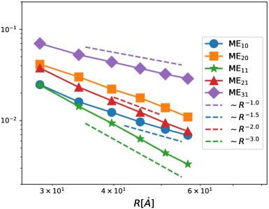
(a) Micro-crack-2

(b) Micro-crack-3

Figure 7.6. Convergence of the relative moments error ${\rm ME}_{ki}$ defined by (4.28) against domain size $R$ for two micro-crack cases.

(a) Micro-crack-2

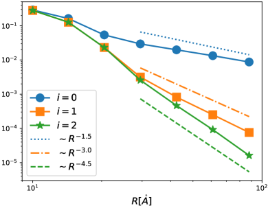
(b) Micro-crack-3

Figure 7.7. Convergence of geometry error $\|D\bar{u}-D\bar{u}_{b_{i}}\|_{\ell^{2}}$ for $i=0,1,2$ against domain size $R$ for two micro-crack cases.

(a) Micro-crack-2

(b) Micro-crack-3

Figure 7.8. Convergence of energy error $\big{|}\mathcal{E}(\bar{u})-\mathcal{E}(\bar{u}_{b_{i}})\big{|}$ for $i=0,1,2$ against domain size $R$ for two micro-crack cases.

References

- [1] D. Barnett. The precise evaluation of derivatives of the anisotropic elastic green’s functions. Phys. Status Solidi B, 49(2):741–748, 1972.
- [2] J. Braun, M. Buze, and C. Ortner. The effect of crystal symmetries on the locality of screw dislocation cores. SIAM J. Math. Anal., 51, 2019.
- [3] J. Braun, T. Hudson, and C. Ortner. Asymptotic expansion of the elastic far-field of a crystalline defect. ArXiv e-prints, 2108.04765, 2021.
- [4] J. Braun and C. Ortner. Sharp uniform convergence rate of the supercell approximation of a crystalline defect. SIAM J. Numer. Anal., 58, 2020.
- [5] Julian Braun and Bernd Schmidt. Existence and convergence of solutions of the boundary value problem in atomistic and continuum nonlinear elasticity theory. Calculus of Variations and Partial Differential Equations, 55(5):1–36, 2016.
- [6] Maciej Buze and James R Kermode. Numerical-continuation-enhanced flexible boundary condition scheme applied to mode-i and mode-iii fracture. Physical Review E, 103(3):033002, 2021.
- [7] H. Chen, F.Q. Nazar, and C. Ortner. Geometry equilibration of crystalline defects in quantum and atomistic descriptions. Math. Models Methods Appl. Sci., 29:419–492, 2019.
- [8] H. Chen, C. Ortner, and Y. Wang. QM/MM methods for crystalline defects. part 3: Machine-learned interatomic potentials. ArXiv e-prints, 2106.14559, 2021.
- [9] M. Daw and M. Baskes. Embedded-atom method: Derivation and application to impurities, surfaces, and other defects in metals. Phys. Rev. B, 29:6443–6453, 1984.
- [10] S. Dudarev and P. Ma. Elastic fields, dipole tensors, and interaction between self-interstitial atom defects in bcc transition metals. Phys. Rev. Mater., 2(3):033602, 2018.
- [11] W. E and Z. Huang. Matching conditions in atomistic-continuum modeling of materials. Phys. Rev. Lett., 87(13):135501, 2001.
- [12] V. Ehrlacher, C. Ortner, and A. Shapeev. Analysis of boundary conditions for crystal defect atomistic simulations. Arch. Ration. Mech. Anal., 222:1217–1268, 2016.
- [13] JD Eshelby. The continuum theory of lattice defects. In Solid state physics, volume 3, pages 79–144. Elsevier, 1956.
- [14] R Gröger, AG Bailey, and V Vitek. Multiscale modeling of plastic deformation of molybdenum and tungsten: I. atomistic studies of the core structure and glide of 1/2¡ 1 1 1¿ screw dislocations at 0 k. Acta Materialia, 56(19):5401–5411, 2008.
- [15] Mark F Horstemeyer. Multiscale modeling: a review. Practical aspects of computational chemistry, pages 87–135, 2009.
- [16] T. Hudson and C. Ortner. On the stability of bravais lattices and their cauchy–born approximations. ESAIM: Math. Model. Numer. Anal., 46(1):81–110, 2012.
- [17] T. Hudson and C. Ortner. Analysis of stable screw dislocation configurations in an anti-plane lattice model. SIAM J. Math. Anal., 41:291–320, 2015.
- [18] T. Hughes. The finite element method: linear static and dynamic finite element analysis. Courier Corporation, 2012.
- [19] D. Liu and J. Nocedal. On the limited memory bfgs method for large scale optimization. Math. Program., 45(1):503–528, 1989.
- [20] M. Luskin and C. Ortner. Atomistic-to-continuum coupling. Acta Numerica, 22:397–508, 2013.
- [21] R. Nazarov, JS. Majevadia, M. Patel, M. Wenman, D. Balint, J. Neugebauer, and A. Sutton. First-principles calculation of the elastic dipole tensor of a point defect: Application to hydrogen in -zirconium. Phys. Rev. B, 94(24):241112, 2016.
- [22] AS Nowick and WR Heller. Anelasticity and stress-induced ordering of point defects in crystals. Advances in Physics, 12(47):251–298, 1963.
- [23] D. Olson, C. Ortner, Y. Wang, and L. Zhang. Theoretical study of elastic far-field decay from dislocations in multilattices. ArXiv e-prints, 1910.12269, 2019.
- [24] J. Reddy. Introduction to the finite element method. McGraw-Hill Education, 2019.
- [25] J. Revels, M. Lubin, and T. Papamarkou. Forward-mode automatic differentiation in julia. arXiv preprint arXiv:1607.07892, 2016.
- [26] JE Sinclair. The influence of the interatomic force law and of kinks on the propagation of brittle cracks. The Philosophical Magazine: A Journal of Theoretical Experimental and Applied Physics, 31(3):647–671, 1975.
- [27] JE Sinclair and BR Lawn. An atomistic study of cracks in diamond-structure crystals. Proceedings of the Royal Society of London. A. Mathematical and Physical Sciences, 329(1576):83–103, 1972.
- [28] Martin Oliver Steinhauser. Computational multiscale modeling of fluids and solids. Springer, 2017.
- [29] E. Tadmor, R. Phillips, and M. Ortiz. Mixed atomistic and continuum models of deformation in solids. Langmuir, 12(19):4529–4534, 1996.
- [30] Anne Marie Z Tan and Dallas R Trinkle. Computation of the lattice green function for a dislocation. Physical Review E, 94(2):023308, 2016.
- [31] Dallas R Trinkle. Lattice green function for extended defect calculations: Computation and error estimation with long-range forces. Physical Review B, 78(1):014110, 2008.
- [32] H. Wang, M. Liao, P. Lin, and L. Zhang. A posteriori error estimation and adaptive algorithm for atomistic/continuum coupling in two dimensions. SIAM J. Sci. Comput., 40(4):A2087–A2119, 2018.
- [33] Y. Wang, H. Chen, M. Liao, C. Ortner, H. Wang, and L. Zhang. A posteriori error estimates for adaptive qm/mm coupling methods. SIAM J. Sci. Comput., 43(4):A2785–A2808, 2021.
- [34] Sidney Yip. Handbook of materials modeling. Springer Science & Business Media, 2007.