Non-Asymptotic Analysis of a UCB-based
Top Two Algorithm
Abstract
A Top Two sampling rule for bandit identification is a method which selects the next arm to sample from among two candidate arms, a leader and a challenger. Due to their simplicity and good empirical performance, they have received increased attention in recent years. However, for fixed-confidence best arm identification, theoretical guarantees for Top Two methods have only been obtained in the asymptotic regime, when the error level vanishes. In this paper, we derive the first non-asymptotic upper bound on the expected sample complexity of a Top Two algorithm, which holds for any error level. Our analysis highlights sufficient properties for a regret minimization algorithm to be used as leader. These properties are satisfied by the UCB algorithm, and our proposed UCB-based Top Two algorithm simultaneously enjoys non-asymptotic guarantees and competitive empirical performance.
1 Introduction
Faced with a collection of items (“arms”) with unknown probability distributions, a question that arises in many applications is to find the distribution with the largest mean, which is referred to as the best arm. Different approaches have been considered depending on the data collection process. Sequential hypothesis testing [10, 37] encompasses situations where there is no control on the collected samples. Experimental design [7, 35] aims at choosing the data collection scheme a priori. In the multi-armed bandit [4, 20] and the ranking and selection [18] literature, an algorithm chooses sequentially the distribution from which it will collect an additional sample based on past data.
In order to have theoretical guarantees for this identification problem, one should adopt a statistical model on the underlying distributions. While parametric models are reasonable for applications such as A/B testing [28], they are unrealistic in other fields such as agriculture [21]. Despite the restricted scope of its applications, studying the identification task for Gaussian distributions is a natural first step. Hopefully the insights gained will then be generalized to wider classes of distributions.
In the fixed confidence identification problem, an algorithm aims at identifying the best arm with an error of at most while using as few samples as possible. Since each sample has a cost, those algorithms should provide an upper bound on the expected number of samples used by the algorithm before stopping. For those guarantees to be useful in practice, they should hold for any , which is referred to as the non-asymptotic (or moderate) regime. In contrast, the asymptotic regime considers vanishing error level, i.e. . For Gaussian distributions, Top Two algorithms [36, 39] have only been studied in the asymptotic regime. We show the first non-asymptotic guaranty for a Top Two algorithm holding for any instance with a unique best arm.
1.1 Setting and related work
A Gaussian bandit problem is described by arms whose probability distributions belongs to the set of Gaussian distributions with known variance . By rescaling, we assume for all . Since an element of is uniquely characterized by its mean, the vector refers to a -arms Gaussian bandit. Let be the -dimensional simplex.
A best arm identification (BAI) algorithm aims at identifying an arm with highest mean parameter, i.e. an arm belonging to the set . At each time , the algorithm (1) chooses an arm based on previous observations, (2) observes a sample , and (3) decides whether it should stop and return an arm or continue sampling. We consider the fixed confidence identification setting, in which the probability of error of an algorithm is required to be less than a given on all instances . The sample complexity of an algorithm corresponds to its stopping time , which counts the number of rounds before termination. An algorithm is said to be -correct on if for all [14]. We aim at designing -correct algorithms minimizing .
As done in all the literature on fixed-confidence BAI, we assume that there is a unique best arm and we denote it by or when is clear from the context. To ensure -correctness on , an algorithm has to be able to distinguish the unknown from any instance having a different best arm, hence it needs to estimates the gaps between arms. Lemma 1.1 gives a lower bound on the expected sample complexity which is known to be tight in the asymptotic regime, i.e. when goes to zero.
Lemma 1.1 ([17]).
An algorithm which is -correct on all problems in satisfies that for all , where and, for all ,
When considering the sub-class of algorithms allocating a fraction of their sample to the best arm, we obtain a lower bound as in Lemma 1.1 with instead of . An algorithm is said to be asymptotically optimal (resp. -optimal) if its sample complexity matches that lower bound asymptotically, that is if (resp. ). [38] showed the worst-case inequality for any single-parameter exponential families. Therefore, the expected sample complexity of an asymptotically -optimal algorithm with is at worst twice higher than that of any asymptotically optimal algorithm. Leveraging the symmetry of Gaussian distributions, a tighter worst-case inequality can be derived (Lemma C.6). The allocations and realizing and are known to be unique, and satisfy . [6] showed that for Gaussian distributions (Lemma C.4).
Related work
The first BAI algorithms were introduced and studied under the assumption that the observation have bounded support, with a known upper bound [15, 24, 16, 19]. The sample complexity bounds proved for these algorithms scale as the sum of squared inverse gap, i.e. where , which satisfies [17]. Following their work, a rich literature designed asymptotically optimal algorithms in the fixed-confidence setting for parametric distributions, such as single-parameter exponential families, and non-parametric distributions such as bounded ones. Those algorithms build on two main ideas. The Tracking approach computes at each round the optimal allocation for the empirical estimator, and then tracks it [17]. To achieve lower computational cost, Game-based algorithms [12] view as a min-max game between the learner and the nature, and design saddle-point algorithms to solve it sequentially.
Top Two algorithms arose as an identification strategy based on the Thompson Sampling algorithm for regret minimization [41]: [38] introduced Top Two Probability Sampling (TTPS) and Top Two Thompson Sampling (TTTS). Adopting a Bayesian viewpoint, Russo studied the convergence rate of the posterior probability that is not the best arm, under some conditions on the prior. For Gaussian bandits, other Bayesian Top Two algorithms with frequentist components have been shown to be asymptotically -optimal: Top Two Expected Improvement (TTEI, [36]) and Top Two Transportation Cost (T3C, [39]). [21] introduces fully frequentist Top Two algorithms. Their analysis proves asymptotic -optimality for several Top Two algorithms and distribution classes, beyond Gaussian. [34] provides guarantees for single-parameter exponential families, at the price of adding forced exploration. [44] proposes an algorithm to tackle the top- identification problem and introduces information-directed selection (IDS) to choose in an adaptive manner, which differs from the one proposed in [33]. In addition to their success in the fixed-confidence setting, Top Two algorithms have also been studied for fixed-budget problems [2], in which guarantees on the error probability should be given after samples. While existing Top Two sampling rules differ by how they choose the leader and the challenger, they all sample the leader with probability . By design, Top Two algorithms with a fixed can reach -optimality at best, and cannot be optimal on all instances .
Shortcomings of the asymptotic regime
While the literature provides a detailed understanding of the asymptotic regime, many interesting questions are unanswered in the non-asymptotic regime. Recent works [9, 40, 32, 31] have shown that the sample complexity is affected by strong moderate confidence terms (independent of ). The analysis of [21] applies to their -EB-TC algorithm whose empirical stopping times is order of magnitude larger than its competitors for . Since the proof of asymptotic -optimality hides design flaws, non-asymptotic guarantees should be derived to understand which Top Two algorithms will perform well in practice for any reasonable choice of .
1.2 Contributions
Our main contribution is to propose the first non-asymptotic analysis of Top Two algorithms. We identify sufficient properties of the leader (seen as a regret-minimization algorithm) for it to hold. This solves two open problems: obtaining an upper bound which (1) is non-asymptotic (Theorem 2.4 holds for any ) and (2) holds for all instances having a unique best arm (i.e. sub-optimal arms can have the same mean, which was not allowed in the analyzes of existing Top Two algorithms). As a consequence, we propose the TTUCB (Top Two UCB) algorithm which builds on the UCB algorithm.
By using tracking instead of sampling to choose between the leader and the challenger, TTUCB is the first Top Two algorithm which is asymptotically -optimal (Theorem 2.3) and has non-asymptotic guarantees (Theorem 2.4). Our experiments reveal that TTUCB performs on par with existing Top Two algorithms, which are only proven to be asymptotically -optimal, even for large sets of arms. Numerically, we show that considering adaptive proportions compared to a fixed yields a significant speed-up on hard instances, and to a moderate improvement on random instances.
2 UCB-based Top Two algorithm
We propose a fully deterministic Top Two algorithm based on UCB [5], named TTUCB and detailed in Algorithm 1. We prove a non-asymptotic upper bound on the expected sample complexity holding for any instance having a unique best arm.
Stopping and recommendation rules
The -algebra encompasses all the information available to the agent before time . Let be the number of pulls of arm before time , and its empirical mean by .
The algorithm stops as soon as the generalized likelihood ratio exceeds a threshold , i.e.
| (1) |
where we recommend at time . Lemma 2.1 provides an explicit threshold ensuring -correctness, which relies on concentration inequalities derived in [27].
Lemma 2.1.
Sampling rule
We initialize by sampling each arms once. At time , a Top Two sampling rule defines a leader and a challenger , and chooses or based on a fixed allocation . In prior work this choice was done at random, which means that the leader was sampled with probability . We replace randomization by tracking, and show similar theoretical and numerical results (see Figure 4 in Appendix G.2). For fixed , we recommend to use without prior knowledge on the unknown mean parameters (see Section 3.4 for adaptive proportions). This recommendation is supported theoretically by the fact that (Lemma C.4) and that is significantly smaller than for most instances (Lemma C.6 and Figure 2).
Let be the number of time arm was the leader, and be the number of pulls of arm at rounds in which was the leader. We use independent tracking procedures. A tracking procedure is a deterministic method to convert a sequence of allocations over arms into a sequence of arms, which ensures that the empirical proportions are close to the averaged allocation over arms. For each leader, we track the allocation between the leader and the challenger. Formally, we set if , else . Using Theorem 6 in [13] for each tracking procedure yields Lemma 2.2.
Lemma 2.2.
For all and all , we have .
Using tracking over randomization is motivated by practical and theoretical reasons. First, in some specific applications, the practitioner might be only willing to use a deterministic algorithm. Second, in the analysis, it is easier to control deterministic counts since it removes the need for martingales arguments to bound the deviations of the samples. Therefore, tracking simplifies the non-asymptotic analysis. Third, Lemma 2.2 shows that the speed of convergence is at least for tracking, while we would obtain a speed of for randomization.
At time , the UCB leader is defined as
| (3) |
where is a bonus coping for uncertainty. Let and be two concentration parameters. The choice of should ensure that we have an upper confidence bound on holding with high probability: with probability , for all and all arms , . For Gaussian observations, a function which is sufficient for the purpose of our proof can be obtained by a union bound over time, giving . We can improve on with mixtures of martingales, yielding with for all , where is the negative branch of the Lambert function, and . A UCB leader with recovers the Empirical Best (EB) leader [21]. Choosing is central for empirical performance and non-asymptotic guarantees, but not for asymptotic ones. The lowest will yield better empirical performance since larger means more conservative confidence bounds. In our experiments where , we will consider since for .
Given a leader , the TC challenger is defined as
| (4) |
where . [39] introduced the TC challenger as a computationally efficient approximation of the challenger in TTTS [38], which uses re-sampling till an unlikely event occurs. Both T3C and TTTS use the TS leader which takes the best arm of a vector of realization drawn from a sampler, e.g. for Gaussian distributions with unit variance.
Computational cost
Computing the stopping rule (1) and the UCB leader (3) can be done in . At time where coincides with , computing the TC challenger (4) is done as a by-product of the computation of the stopping rule, without additional cost. When , we draw at random an arm with larger empirical mean. The per-round computational and memory cost of TTUCB is .
2.1 Sample complexity upper bound
Leveraging the unified analysis of Top Two algorithms proposed by [21], we obtain the asymptotic -optimality of TTUCB (Theorem 2.3). After showing the required properties for the UCB leader, we proved that tracking Top Two algorithms have similar properties as their sampling-based counterparts.
Theorem 2.3.
Theorem 2.3 and guarantees for other Top Two algorithms hold only for arms having distinct means. Moreover, an asymptotic result provides no guarantees on the performance in moderate regime of . We address those two limitations.
Non-asymptotic upper bound
Theorem 2.4 gives an upper bound on the expected sample complexity holding for any and any instance having a unique best arm. It is a direct corollary of a more general result holding for any , and (Theorem D.4).
Theorem 2.4.
The TTUCB sampling rule using in (3) satisfies a similar upper bound (Corollary D.5). Since Theorem 2.4 holds for any instance having a unique best arm, we corroborate the intuition that assuming is an artifact of the existing proof to obtain asymptotic -optimality.
The upper bound on involves several terms. The -dependent term is . In the asymptotic regime, we can show that by taking and letting go to zero. While there is (sub-optimal) factor in , Theorem 2.3 shows that TTUCB is asymptotically -optimal. This factor is a price we paid to obtain more explicit non-asymptotic terms, and removing it would require more sophisticated arguments in order to control the convergence of the empirical proportions towards .
In the regime where , the upper bound is dominated by the -independent term (when ) with satisfies . Compared to the best known upper and lower bounds in this regime (see discussion below), our non-asymptotic term has a sub-optimal scaling in with . While taking would mitigate this sub-optimality, it would yield a larger dependency in . Empirically, Figures 1(b) and 5 (Appendix G.2) hints that the empirical performance of TTUCB has a better scaling with than .
For instances such that is arbitrarily small, taking yields an arbitrarily large . By clipping with , we circumvent this pitfall and ensure that . Since it yields a larger , we are trading-off asymptotic terms for improved non-asymptotic ones. We illustrate this with two archetypal instances. For the “-sparse” instance, in which and for all , we have by symmetry that for all . Therefore, we have since for all . The “almost dense” instance is such that , and for all . By symmetry, there exists a function with , such that and for all . While , we obtain by taking since .
| Algorithm | Asymptotic behavior | Finite-confidence behavior |
|---|---|---|
| LUCB1 [24] | ||
| Exp-Gap [25] | ||
| lil’ UCB [19] | ||
| DKM [12] | ||
| Peace [26] | ||
| FWS [42] | ||
| EBS [6]* | ||
| TTUCB** | with |
Comparison with existing upper bounds
Table 1 summarizes the asymptotic and non-asymptotic scalings of the upper bound on the sample complexity of existing BAI algorithms. Among the class of asymptotically (-)optimal algorithms, very few of them also enjoy non-asymptotic guarantees, e.g. the analyses of Track-and-Stop and Top Two algorithms are asymptotic. The gamification approach of [12] is the first attempt to provide both. Their non-asymptotic upper bound on involves an implicit time which scales with and is only valid for (see Lemma 2, with constants in Appendix D.7). Let . As a first order approximation, they obtain , and we obtain (Lemma D.13). [42] were the first to obtain an upper bound on of the form . While they improved the second-order -dependent term, the -independent term scales with (see their Theorem 2 for , with constants given by Appendix N). The algorithm proposed by [6] has a non-asymptotic upper bound on of the form which is valid for , where is such that . Since , they obtain a better -dependency. However, is arbitrarily large when is arbitrarily small since it scales with . Therefore, they suffer from the pitfall which we avoided by clipping. In light of Table 1, TTUCB enjoys the best scaling when in the class of asymptotically (-)optimal BAI algorithms.
The LUCB1 algorithm [24] has a structure similar to a Top Two algorithm, with the difference that LUCB samples both the leader and the challenger instead of choosing one. As LUCB1 satisfies , it enjoys better scaling when than TTUCB. Since the empirical allocation of LUCB1 is not converging towards , it is not asymptotically -optimal. The Peace algorithm [26] has a non-asymptotic upper bound on of the form holding with probability . The term is a Gaussian-width which originates from concentration on the suprema of Gaussian processes and satisfies .
Another class of BAI algorithms focus on the dependency in the gaps , and derive non-asymptotic upper bound on holding with high probability. [25, 19, 8, 9] gives -PAC algorithms with an upper bound of the form , and [19] shows that for two arms the dependency is optimal when . While those algorithms obtain the best scaling when , they are not asymptotically (-)optimal.
3 Non-asymptotic analysis
3.1 Proof sketch of Theorem 2.4
Existing analyses of Top Two algorithms are asymptotic in nature and requires too much control on the empirical means and proportions to yield any meaningful information in the finite-confidence regime. Therefore, we adopt a different approach which ressembles the non-asymptotic analysis of [12]. We first define concentration events to control the deviations of the random variables used in the UCB leader and the TC challenger. For all , let where
Using Lemmas D.8 and E.6, the proof boils down to constructing a time after which for since it would yield that .
Let such that holds true, and such that . Using that , under , the stopping condition yields that
Let be the unique element of . Lemma 3.1 links the empirical proportions to for . It is the key technical challenge of our non-asymptotic proof strategy.
Lemma 3.1.
Let . There exist such that for all such that holds true, there exists with , which satisfies
Before proving Lemma 3.1, we conclude the proof of Theorem 2.4. Let and as in Lemma 3.1 and . For all , we have . Therefore, we have proved that for all . This concludes the proof.
Provided that , the above only used the stopping condition and the TC challenger, and no other properties of the leader. Lemma 3.2 shows that , except for a sublinear number of times. Section 3.3 exhibits sufficient conditions on a regret minimization algorithm to obtain a non-asymptotic upper bound.
Lemma 3.2.
Under the event , we have .
Proof sketch of Lemma 3.1
The key technical challenge is to link with . We adopt the approach used to analyze of APT [30]: consider an arm being over-sampled and study the last time this arm was pulled. By the pigeonhole principle, at time ,
| (5) |
Let be the last time at which and , hence . Using Lemmas 2.2 and 3.2, we show that , hence for large enough (see Appendix D.2). Then, we need to link to . When is small, (5) can be true at , hence there is no hope to show that . To circumvent this problem, we link to thanks to Lemma 2.2, and use that
for with (Lemmas D.10 and D.11), where lower bounds . This concludes the proof for . The (sub-optimal) multiplicative factor in comes from the inequality (3.1). To remove it, we need to control the deviation between the empirical proportion of arm and for all . Nevertheless, TTUCB is asymptotically -optimal (Theorem 2.3).
Refined analysis
For , we clip by (see Appendix D). Our method can be used to analyze other algorithms, and it improves existing results on APT.
3.2 Beyond Gaussian distributions
Theorems 2.3 and 2.4 hold for sub-Gaussian r.v. thanks to direct adaptations of concentration results (Lemmas 2.1, E.2 and E.5). The situation is akin to the regret bound of UCB: it holds for any sub-Gaussian, but it is close to optimality in a distribution-dependent sense only for Gaussians. However, if the focus is on asymptotically -optimal algorithms, then it is challenging to express the characteristic time for the non-parametric class of sub-Gaussian distributions.
The TTUCB algorithm can also be defined for more general distributions such as single-parameter exponential families or bounded distributions. It is only a matter of adapting the definition of the UCB leader and the TC challenger. For bounded distributions, the UCB leader was studied in [1] and the TC challenger was analyzed in [21]. Leveraging their unified analysis of Top Two algorithms with our tracking-based results, we can show asymptotic -optimality of TTUCB for bounded distributions and single-parameter exponential families with sub-exponential tails. We believe that non-asymptotic guaranties could be obtained for more general distributions, but it will come at the price of more technical arguments and less explicit non-asymptotic terms.
3.3 Generic regret minimizing leader
Our non-asymptotic analysis highlights that any regret minimization algorithm that selects the arm except for a sublinear number of times (Property 1) can be used as leader with the TC challenger.
Property 1.
There exists with and a function with for some such that under event , .
For asymptotic guarantees, the sufficient properties on the leader from [21] are weaker since they are even satisfied by the greedy choice . While Top Two algorithms were introduced by [38] to adapt Thompson Sampling to BAI, we have shown that other regret minimization algorithms can be used: the Top Two method is a generic wrapper to convert any regret minimization algorithm into a best arm identification strategy.
The regret of an algorithm at time , , is almost always studied through its expectation . This is however not sufficient for our application. We need to prove that with high probability, is small for all arm . Such guarantees are known for UCB [3] and ETC [29], but are yet unknown for Thompson Sampling. We cannot in general obtain a good enough bound on from a bound on . However, we can if we have high probability bounds on . Suppose that a regret minimization algorithm satisfies Property 2 and is independent of the horizon .
Property 2.
There exists , , with and a function with such that under event , .
Let be the algorithm used in a Top Two procedure, but which uses only the observations obtained at times such that and discards the rest. Let and . Then, under , satisfies and Lemma 2.2 yields . Therefore, Property 1 holds for and . Given a specific algorithm, a finer analysis could avoid discarding information by using with every observations.
3.4 Adaptive proportions
Given a fixed allocation , any Top Two algorithm can at best be asymptotically -optimal. Since the optimal allocation is unknown, it should be learned from the observations by a Top Two algorithm using an adaptive proportion at time . Recently, [44] proposes IDS to choose in an adaptive manner. For BAI with Gaussian observations, IDS yields . Let be the average proportion when arm was the leader before time . Tracking with IDS requires to use instead of . Using the analysis of [44], it is reasonable to believe that one could obtain asymptotic optimality of TTUCB with IDS. However it is not clear how to adapt the non-asymptotic analysis since it heavily relies on being fixed and bounded away from . Experiments with IDS are available in Appendix G.2.1.
4 Experiments
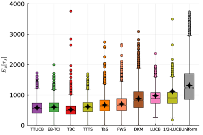
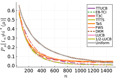
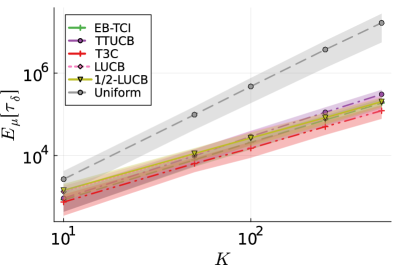
In the moderate regime (), we assess the empirical performance of TTUCB with bonus and concentration parameters . As benchmarks, we compare our algorithm with three sampling-based Top Two algorithms: TTTS, T3C and -EB-TCI. In addition, we consider Track-and-Stop (TaS) [17], FWS [42], DKM [12], LUCB [24] and uniform sampling. At time , the LUCB algorithm computes a leader and a challenger, then sample them both (see Appendix G.1). To provide a clear comparison with Top Two algorithms, we define a new -LUCB algorithm which sample the leader with probability , else sample the challenger. At the exception of LUCB and -LUCB which have their own stopping rule, all algorithms uses the stopping rule (1) with the heuristic threshold . Even though this choice is not sufficient to prove -correctness, it yields an empirical error which is several orders of magnitude lower than . Top Two algorithms and -LUCB use . To allow for a fair numerical comparison, LUCB and -LUCB use as bonus, which is too tight to yield valid confidence intervals. Supplementary experiments are available in Appendix G.
Random instances
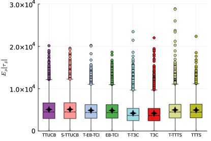
We assess the performance on random Gaussian instances with such that and for all . Numerically, we observe (mean std). In Figure 1(a), we see that TTUCB performs on par with existing Top Two algorithms, and slightly outperforms TaS and FWS. Our algorithm achieves significantly better result than DKM, LUCB, -LUCB and uniform sampling. The CPU running time is reported in Table 4, and the observed empirical errors before stopping is displayed in Figure 3 (Appendix G.2).
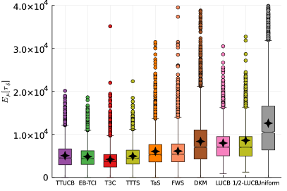
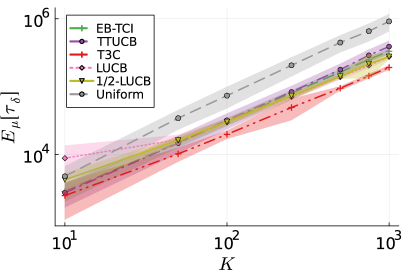
Larger sets of arms
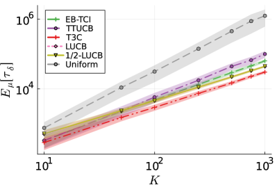
We evaluate the impact of larger number of arms. The “-sparse” scenario of [20] sets and for all , i.e. (see Appendix G.2 for other instances). We consider algorithms with low computational cost. In Figure 1(b), all algorithms have the same linear scaling in (i.e. in ). Faced with an increase in the number of arms, the TS leader used in T3C appears to be more robust than the UCB leader in TTUCB. This is a common feature of UCB algorithms which have to overcome the bonus of sub-optimal arms.
5 Conclusion
In this paper, we have shown the first non-asymptotic upper bound on the expected sample complexity of a Top Two algorithm, which holds for any error level and for any instance having a unique best arm. Furthermore, we have demonstrated that the TTUCB algorithm achieves competitive empirical performance compared to other algorithms, including Top Two methods.
While our guarantees hold for a fixed proportion allocated to the leader, [44] recently introduced IDS to define an adaptive proportion at time and show asymptotic optimality for Gaussian distributions. Deriving guarantees for IDS for single-parameter exponential families is a challenging open problem. Finally, Top Two algorithms are a promising method to tackle complex settings. While heuristics exist for some structured bandits such as Top-, it would be interesting to efficiently adapt Top Two methods to deal with sophisticated structure, e.g. linear bandits.
Acknowledgments and Disclosure of Funding
Experiments presented in this paper were carried out using the Grid’5000 testbed, supported by a scientific interest group hosted by Inria and including CNRS, RENATER and several Universities as well as other organizations (see https://www.grid5000.fr). This work has been partially supported by the THIA ANR program “AI_PhD@Lille”. The authors acknowledge the funding of the French National Research Agency under the project FATE (ANR22-CE23-0016-01).
References
- Agrawal et al. [2021] S. Agrawal, S. K. Juneja, and W. M. Koolen. Regret minimization in heavy-tailed bandits. In Conference on Learning Theory, 2021.
- Ariu et al. [2021] K. Ariu, M. Kato, J. Komiyama, K. McAlinn, and C. Qin. Policy choice and best arm identification: Asymptotic analysis of exploration sampling under posterior weighted policy regret. arXiv preprint arXiv:2109.08229, 2021.
- Audibert et al. [2009] J.-Y. Audibert, R. Munos, and C. Szepesvári. Exploration-exploitation trade-off using variance estimates in multi-armed bandits. Theoretical Computer Science, 410(19), 2009.
- Audibert et al. [2010] J.-Y. Audibert, S. Bubeck, and R. Munos. Best Arm Identification in Multi-armed Bandits. In Conference on Learning Theory, 2010.
- Auer et al. [2002] P. Auer, N. Cesa-Bianchi, and P. Fischer. Finite-time analysis of the multiarmed bandit problem. Machine Learning, 47(2):235–256, 2002.
- Barrier et al. [2022] A. Barrier, A. Garivier, and T. Kocák. A non-asymptotic approach to best-arm identification for gaussian bandits. In Proceedings of The 25th International Conference on Artificial Intelligence and Statistics, 2022.
- Chaloner and Verdinelli [1995] K. Chaloner and I. Verdinelli. Bayesian experimental design: A review. Statistical Science, 1995.
- Chen et al. [2017a] L. Chen, J. Li, and M. Qiao. Towards instance optimal bounds for best arm identification. Conference on Learning Theory, 2017a.
- Chen et al. [2017b] L. Chen, J. Li, and M. Qiao. Nearly instance optimal sample complexity bounds for top-k arm selection. In Artificial Intelligence and Statistics, 2017b.
- Chernoff [1959] H. Chernoff. Sequential design of Experiments. The Annals of Mathematical Statistics, 30(3):755–770, 1959.
- Degenne [2019] R. Degenne. Impact of structure on the design and analysis of bandit algorithms. PhD thesis, Université de Paris, 2019.
- Degenne et al. [2019] R. Degenne, W. M. Koolen, and P. Ménard. Non-asymptotic pure exploration by solving games. In Advances in Neural Information Processing Systems (NeurIPS), 2019.
- Degenne et al. [2020] R. Degenne, H. Shao, and W. M. Koolen. Structure adaptive algorithms for stochastic bandits. In International Conference on Machine Learning (ICML), 2020.
- Even-Dar et al. [2002] E. Even-Dar, S. Mannor, and Y. Mansour. Pac bounds for multi-armed bandit and markov decision processes. In International Conference on Computational Learning Theory, 2002.
- Even-Dar et al. [2006] E. Even-Dar, S. Mannor, and Y. Mansour. Action Elimination and Stopping Conditions for the Multi-Armed Bandit and Reinforcement Learning Problems. Journal of Machine Learning Research, 7:1079–1105, 2006.
- Gabillon et al. [2012] V. Gabillon, M. Ghavamzadeh, and A. Lazaric. Best Arm Identification: A Unified Approach to Fixed Budget and Fixed Confidence. In Advances in Neural Information Processing Systems, 2012.
- Garivier and Kaufmann [2016] A. Garivier and E. Kaufmann. Optimal best arm identification with fixed confidence. In Proceedings of the 29th Conference On Learning Theory, 2016.
- Hong et al. [2021] L. Hong, W. Fan, and J. Luo. Review on ranking and selection: A new perspective. Frontiers of Engineering Management, 8:321–343, 2021.
- Jamieson et al. [2014] K. Jamieson, M. Malloy, R. Nowak, and S. Bubeck. lil’UCB: an Optimal Exploration Algorithm for Multi-Armed Bandits. In Proceedings of the 27th Conference on Learning Theory, 2014.
- Jamieson and Nowak [2014] K. G. Jamieson and R. D. Nowak. Best-arm identification algorithms for multi-armed bandits in the fixed confidence setting. In Conference on Information Sciences and Systems (CISS), 2014.
- Jourdan et al. [2022] M. Jourdan, R. Degenne, D. Baudry, R. De Heide, and E. Kaufmann. Top two algorithms revisited. Advances in Neural Information Processing Systems, 2022.
- Jourdan et al. [2023] M. Jourdan, R. Degenne, and E. Kaufmann. Dealing with unknown variances in best-arm identification. International Conference on Algorithmic Learning Theory, 2023.
- Jun and Nowak [2016] K.-W. Jun and R. Nowak. Anytime exploration for multi-armed bandits using confidence information. In International Conference on Machine Learning (ICML), 2016.
- Kalyanakrishnan et al. [2012] S. Kalyanakrishnan, A. Tewari, P. Auer, and P. Stone. PAC subset selection in stochastic multi-armed bandits. In International Conference on Machine Learning (ICML), 2012.
- Karnin et al. [2013] Z. Karnin, T. Koren, and O. Somekh. Almost optimal Exploration in multi-armed bandits. In International Conference on Machine Learning (ICML), 2013.
- Katz-Samuels et al. [2020] J. Katz-Samuels, L. Jain, K. G. Jamieson, et al. An empirical process approach to the union bound: Practical algorithms for combinatorial and linear bandits. Advances in Neural Information Processing Systems, 2020.
- Kaufmann and Koolen [2021] E. Kaufmann and W. M. Koolen. Mixture martingales revisited with applications to sequential tests and confidence intervals. Journal of Machine Learning Research, 22(246):1–44, 2021.
- Kaufmann et al. [2014] E. Kaufmann, O. Cappé, and A. Garivier. On the Complexity of A/B Testing. In Proceedings of the 27th Conference On Learning Theory, 2014.
- Lattimore and Szepesvari [2019] T. Lattimore and C. Szepesvari. Bandit Algorithms. Cambridge University Press, 2019.
- Locatelli et al. [2016] A. Locatelli, M. Gutzeit, and A. Carpentier. An optimal algorithm for the thresholding bandit problem. In International Conference on Machine Learning (ICML), 2016.
- Marjani et al. [2022] A. A. Marjani, T. Kocák, and A. Garivier. On the complexity of all -best arms identification. In Joint European Conference on Machine Learning and Knowledge Discovery in Databases, 2022.
- Mason et al. [2020] B. Mason, L. Jain, A. Tripathy, and R. Nowak. Finding all -good arms in stochastic bandits. Advances in Neural Information Processing Systems, 2020.
- Mukherjee and Tajer [2023a] A. Mukherjee and A. Tajer. Best arm identification in stochastic bandits: Beyond -optimality. arXiv preprint arXiv:2301.03785, 2023a.
- Mukherjee and Tajer [2023b] A. Mukherjee and A. Tajer. Sprt-based efficient best arm identification in stochastic bandits. IEEE Journal on Selected Areas in Information Theory, 2023b.
- Pukelsheim [2006] F. Pukelsheim. Optimal design of experiments. SIAM, 2006.
- Qin et al. [2017] C. Qin, D. Klabjan, and D. Russo. Improving the expected improvement algorithm. In Advances in Neural Information Processing Systems 30 (NIPS), 2017.
- Robbins [1952] H. Robbins. Some aspects of the sequential design of experiments. Bulletin of the American Mathematical Society, 58(5):527–535, 1952.
- Russo [2016] D. Russo. Simple Bayesian algorithms for best arm identification. In Proceedings of the 29th Conference on Learning Theory (COLT), 2016.
- Shang et al. [2020] X. Shang, R. de Heide, E. Kaufmann, P. Ménard, and M. Valko. Fixed-confidence guarantees for bayesian best-arm identification. In International Conference on Artificial Intelligence and Statistics (AISTATS), 2020.
- Simchowitz et al. [2017] M. Simchowitz, K. Jamieson, and B. Recht. The simulator: Understanding adaptive sampling in the moderate-confidence regime. In Conference on Learning Theory, 2017.
- Thompson [1933] W. Thompson. On the likelihood that one unknown probability exceeds another in view of the evidence of two samples. Biometrika, 25:285–294, 1933.
- Wang et al. [2021] P.-A. Wang, R.-C. Tzeng, and A. Proutiere. Fast pure exploration via frank-wolfe. Advances in Neural Information Processing Systems, 2021.
- Wilson [1927] E. B. Wilson. Probable inference, the law of succession, and statistical inference. Journal of the American Statistical Association, 22(158):209–212, 1927.
- You et al. [2023] W. You, C. Qin, Z. Wang, and S. Yang. Information-directed selection for top-two algorithms. In The Thirty Sixth Annual Conference on Learning Theory, pages 2850–2851. PMLR, 2023.
Appendix A Outline
The appendices are organized as follows:
| Notation | Type | Description |
|---|---|---|
| Number of arms | ||
| Mean of arm | ||
| Vector of means, | ||
| Best arm operator, | ||
| Asymptotic (-)characteristic time | ||
| Asymptotic (-)optimal allocation |
Appendix B Notation
We recall some commonly used notation: the set of integers , the complement and interior of a set , Landau’s notation , , and , the -dimensional probability simplex . While Table 2 gathers problem-specific notation, Table 3 groups notation for the algorithms. We emphasize that is the number of times where we pulled arm as a leader before time .
| Notation | Type | Description |
|---|---|---|
| Leader at time | ||
| Challenger at time | ||
| Arm sampled at time | ||
| Proportion parameter | ||
| Sample observed at the end of time , i.e. | ||
| History before time , i.e. | ||
| Arm recommended before time , i.e. | ||
| Sample complexity (stopping time of the algorithm) | ||
| Arm recommended by the algorithm | ||
| Stopping threshold function | ||
| Number of pulls of arm before time , | ||
| Empirical mean of arm before time , | ||
| Counts of before time , | ||
| Counts of before time , |
Appendix C Characteristic times
Let such that . Let and be the unique allocation -optimal allocation satisfying for all (Lemma C.2), i.e. where
We restate without proof two fundamental results on the characteristic time and the associated allocation, which were first shown in [38]. Lemma C.1 gives an upper bound on and Lemma C.2 shows that the (-)optimal allocation is unique with strictly positive values. [38] shows that these two results hold for any single-parameter exponential families. [21] extended their proof for the non-parametric family of bounded distributions. Moreover, they argue that these results should hold for more general distributions provided some regularity assumptions are satisfied.
Lemma C.1 ([38]).
and with ,
Lemma C.2 ([38]).
If is a singleton and , then and are singletons, i.e. the optimal allocations are unique, and and for all .
Gaussian distributions
Since Lemma C.1 is a worst-case inequality holding for general distributions, we expect that tighter inequality can be achieved for Gaussian distributions by leveraging their symmetry. This intuition is fueled by recent results of [6]. Using a rewriting of the optimization problem underlying (Lemma C.3), they provide a better understanding of characteristic times and their optimal allocations (Lemma C.4). In particular, for Gaussian distributions, Lemma C.4 shows that the optimal allocation of arm is never above and is larger than .
Lemma C.3 (Proposition in [6]).
Let be a -arms Gaussian bandits and be the solution of , where
and is convex and decreasing. Then,
Lemma C.4 (Proposition in [6]).
Let be a -arms Gaussian bandits. For ,
For , we have
and
where . In particular, the equalities and are reached if and only if for all .
By inspecting the proof of Proposition 8 in [6], we obtain directly the following rewriting of .
Lemma C.5.
Let be a -arms Gaussian bandits and be the solution of , where
and is convex and decreasing. Then,
Proof.
Using the proof of Proposition 8 in [6], we obtain directly that
where is the solution of where
The idea behind the above result is that at the equilibrium, i.e. at , all the transportation costs are equal to . Then, the implicit equation defining is obtained by using the constraints that . To conclude, we simply use .
Since it is the sum of convex and decreasing functions, is also convex and decreasing. ∎
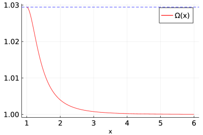
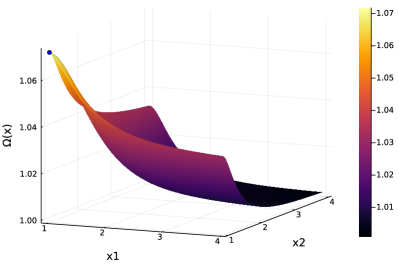
Lemma C.6 aims at improving the worst-case inequality between and in the Gaussian setting. For , those two quantities are equal. For , we showed that is at least , which is achieved when all sub-optimal arms have the same mean. As the gradient of the ratio is the null vector for those instances, we conjecture this is the maximum, i.e. . Our conjecture is supported by numerical simulations for . In Figure 2, we plot the ratio of characteristic times for . We observed that our conjecture is validated empirically, and that is often close to .
Lemma C.6.
For , we have . For , let . Then, for all such that is unique, we have where for all with . In other words, is independent from and . Moreover, we have
Proof.
Using Lemma C.4, we have directly for .
For , we want to upper bound . If we denote by , it is easy to see that when . Likewise, this ratio is invariant by translation of all means by a same quantity. Therefore, we consider without restriction an instance such that and with
where and for all .
First, we can rewrite
where the inequality is an equality if and only for all . Using Lemma C.4, we know that
if and only for all . Therefore, we have exhibited an instance such that
Applying Lemma C.5 for , we obtain where is the implicit solution of the equation
Using Lemma C.3, we know that
where is the implicit solution of the equation
Therefore, we obtain that
and our goal is to show that the above quantity is maximum if and only for all . One way of doing this is by computing the gradient and showing it is negative, which would imply that the function is decreasing. Let . Using the implicit differentiation theorem, we obtain
and
Direct computations yield that
and
and, for s.t. ,
Then, plugging everything together, we obtained that
Therefore, we have shown that . ∎
Appendix D Non-asymptotic analysis
In Appendix D.1, we state and prove one key result for each one of the three main components of the TTUCB sampling rule: the UCB leader (Lemma D.1), the TC challenger (Lemma D.2) and the tracking (Lemma D.3). The proof of Theorem 2.4 is detailed in Appendix D.2, which uses the stopping rule (1) and a proof method from [30]. It is a direct consequence of a more general result (Theorem D.4). In Appendix D.3, we prove a non-asymptotic upper bound for the TTUCB when using instead of (Corollary D.5). We compare our results with uniform sampling in Appendix D.4 (Theorem D.6). Other technicalities are gathered in Appendix D.5.
D.1 Key properties
Before delving in the proof of Theorem D.4 itself, we present the key properties of each component of the TTUCB sampling rule under a some concentration event.
Let and . Let be the sequence of concentration events defined as for all where and are defined in (17) and (19) as
with . In Lemma E.6, it is shown that .
UCB leader
Lemma D.1 shows that the UCB leader is different from for only a sublinear number of times under a certain concentration event. It is slightly more general than Lemma 3.2 presented in Section 2, which follows from .
Lemma D.1.
Proof.
Suppose that at time , the UCB leader is different from , i.e. . Using the event and the definition of yields
We get that if , then . Therefore, we obtain the following upper bound on the number of times the leader is different from up to time
where we used Lemma D.3 for the second inequality and for the third. This concludes the proof for . The same reasoning can be applied for . ∎
TC challenger
Lemma D.2 shows a lower bound on the “transportation” costs used by the TC challenger provided a certain concentration holds. This lower bound depends only on the empirical counts when the best arm is the leader.
Lemma D.2.
For all , under the event , for all such that ,
Proof.
Under , using yields
where the second inequality uses that for all . ∎
Tracking
Lemma D.3 shows the key property satisfied by the independent tracking procedures used by the TTUCB sampling rule. It is slightly more general than Lemma 2.2 presented in Section 2. It is a simple corollary of Theorem 6 in [13].
Lemma D.3.
For all and , we have and for all ,
Proof.
We can rewrite the tracking condition as
For all , this corresponds to a two-arms C-Tracking between the leader and the challengers with for all such that . The leader’s pulling count is and the challengers’ pulling count is . We recall that C-Tracking was defined as .
Theorem 6 in [13] yields for all , . The parallel tracking procedures are independent since they are considering counts partitioned on the considered leader. Therefore, the above results holds for all . This concludes the first part of the proof.
Direct manipulations yield the second part of the result, namely
∎
The choice of independent tracking procedures was made for two reasons. First, independent procedures are simpler to analyze for theoretical purpose. Second, independent procedures yields better empirical performance since it avoids over-sampling a sub-optimal arm when it is mistakenly chosen as leader. To understand the second argument, let’s look at another design with one tracking procedure. Namely we set if , else . When , then it will (almost always) take since is lower than . On the other hand, when with independent tracking procedures, both and are small, hence it is less systematic.
D.2 Proof of Theorem 2.4
Theorem D.4.
Let such that holds true and the algorithm has not stop yet, i.e. . Let such that . Let as in (2), which satisfies that is increasing. Using the stopping rule (1) and , we obtain
The last inequality is an equality when , and trivially true when since a positive term is higher than zero (already null when taking ). Using Lemma D.2, we obtain
where the second inequality is obtained by artificially making appear and taking the minimum of . The last inequality simply uses the definition of .
While combining Lemma D.1 and Lemma D.3 links with , we need another argument to compare the empirical allocation of the sub-optimal arm with its -optimal allocation . Before delving into this key argument, we conclude the proof under an assumption that will be shown to hold later: there exists and such that for all , there exists a well chosen with , which satisfies
| (7) |
Let’s define
For all , the lower bound on is positive, hence we can use that it is upper bounded by . Putting everything together, we have shown that
Therefore, we have (i.e. ) for all . Using that is an decreasing function (since is increasing), we obtain that .
At this stage, the proof of Theorem D.4 boils down to exhibiting and such that: for all , there exists a well chosen with and such that (7) holds. As mentioned above, the crux of the problem is to relate and . To do so, we will build on the idea behind the proof for APT from [30]: consider an arm being over-sampled and study the last time this arm was pulled.
By the pigeonhole principle, at time , there is an index such that (5) holds, i.e.
and we take such . Let be the last time at which was the leader and was the challenger. If then , else . In both cases, we have . Let as in (14). Combined the above with Lemma D.9, we obtain
Let be a lower bound on , for example consider . Let
| (8) |
Since , we obtain that for all . For instances such that is small, the equation (5) can be satisfied at the very beginning, hence might be sublinear in . Therefore, while combining Lemma D.1 and Lemma D.3 yields , it is not possible to obtain . Due to the missing link between and , we use the following inequality
which is a suboptimal step which artificially introduces , and is responsible for the multiplicative factor in Theorem D.4. Improving on this suboptimal step is an interesting question, whose answer still eludes us. One idea would be to leverage the information of the sampled arm at time since we have when , else .
Let . It remains to control both terms. First, we obtain
for all . The last inequality is obtained by definition of
| (9) |
which ensures that, for all , the last condition of the equivalence
is satisfied since and . Second, using Lemma D.3 with , we obtain
for all . The last inequality is obtained by definition of
| (10) |
which ensures that, for all , the last condition of the equivalence
is satisfied since and . By comparison between (8) and (10), we notice that
Putting everything together, we have shown that taking , we have for all , there exists with and such that (7) holds. Let defined in (15). Since , using Lemmas D.10 and D.11 with the above yields
Using yields the first part of Theorem D.4, i.e. the special case of .
Refined non-asymptotic upper bound
When considering large or instances with unbalanced -optimal allocation, can become arbitrarily small. Therefore, the dependency in the inverse of is undesired, and we would like to clip it with a value of our choosing which is away from zero.
Let be an allocation threshold and be the number of arms having a -optimal allocation strictly smaller than . As discussed above, for instances such that (defined above) is small, the equation (5) can be satisfied at the very beginning for a small empirical allocation . To provide a more meaningful result, one needs to have a sub-optimal arm such that either:
-
•
Case 1: is not too small, i.e. .
-
•
Case 2: is too small but is large enough, i.e. and .
In case 1, we can conduct the same manipulations as above simply by using instead of , since it is a lower bound for .
In case 2, the above proof can also be applied by conducting the same algebraic manipulations with instead of , and using . To slightly detail the argument, we can show similarly that , where as in (14) since we have . Then, for all ,
The problematic situation happens when we are neither in case 1 nor in case 2:
-
•
Case 3: both and are too small, i.e. and .
In case 3 it is not possible to conclude the proof with the arm without paying the price of an inverse of . To overcome this price, we need to find another arm such that either case 1 or case 2 happens. Since and are small, we will ignore arm and use the pigeonhole principle on all arm . As in (5), we obtain that there exists such that
where the last inequality is obtained by using and . Based on the same dichotomy happens: either we can conclude the proof when we are in case 1 or 2 or we cannot since we are in case 3. If case 3 occurs also for , i.e. and , we should also ignore it since it is non informative.
The main idea is then to peel off arms that are not informative, till we find an informative one. By induction, we construct a sequence of such arms, where is the first arm for which either case 1 or case 2 holds. This means that for all , we have and
The construction, which rely on the pigeonhole principle for , yields that satisfies
where the last inequality is obtained since and by a simple recurrence on the arms . Since the arm satisfies case 1 or case 2, we can conclude similarly as above. Let .
When , the above proof can also be applied by conducting the same algebraic manipulations with , and using . In more details, we can show that , where as in (14) since we have . Then, for all ,
This allow to conclude the result with , hence paying a multiplicative factor of .
When and , we conclude similarly by manipulating , and using . First, we have , where as in (14) since we have . Then, for all ,
This allow to conclude the result with .
To remove the dependency in the random variable , we consider the worst case scenario where , i.e. . In words, it means that we had to enumerate over all arms with small allocation, such that case 2 didn’t hold, before finding an arm with large allocation, i.e. satisfying case 1.
In all the cases considered above, the parameters always satisfied and . This yields the second part of Theorem D.4, i.e. for .
D.3 Tighter UCB leader
While Theorem 2.3 holds for the TTUCB sampling rule using and , Theorem D.4 is formulated solely for . Experiments highlight that using leads to worse performances than when using . This is not surprising since is smaller than .
It is direct to see that the proof of Theorem D.4 also holds for up to additional technicalities which we detail below. As the obtained non-asymptotic upper bound is less explicit, we chose not to include it in Theorem 2.3.
Let and . Let be the sequence of concentration events defined as for all where is defined in (18) as
where for all , with is the negative branch of the Lambert function.
Let such that holds true and the algorithm has not stop yet, i.e. . Using the second part of Lemma D.1, the vast majority of the proof is unchanged. Modifying the definition of in (14) of Lemma D.9 to account for , we define for all .
In light of the proofs of the technical Lemmas D.10 and D.11, we can define
and obtain directly Corollary D.5 with the same proof as in Appendix D.2.
Corollary D.5.
Explicit upper bound
Since is itself a non-standard function (like logarithm), it is not straightforward to obtain an explicit upper bound on (11). For , it was done in Lemma D.10 by using Lemma D.7.
Using Lemma D.7, we obtain that
where we used , , , and define
| (12) |
For both equivalences above, we used that we are interested in larger values of , hence we used that , , and . Since those conditions are implied by , those conditions are neither restrictive nor informative.
D.4 Uniform sampling
While the shortcomings of uniform sampling are well known for general bandit instances, it is also clear that uniform sampling perform well for highly symmetric instances such that . Therefore, we derive a non-asymptotic upper bound for uniform sampling (Theorem D.6), which allow a clear comparison with Theorem D.4 (and Corollary D.5).
Theorem D.6.
Proof.
Let such that holds true and the algorithm has not stop yet, i.e. . Let . Using the stopping rule (1) and , we obtain
where . Since we sample uniformly, for all time such that , we have for all . Combining the above with Lemma D.2, we obtain
where the last inequality is obtained by taking the minimum over . To conclude the proof, we simply have to link with . More precisely, we will show that and for large enough. By concentration, we have
Therefore, we have , i.e. , for all where
which means that we have at worse . For , we obtain .
Let and . Assume that . Using the definition of and Lemma D.7, direct manipulations yields
where the last inequality uses that and , which is not restrictive (or informative) since it is implied by . When , which means that the problem is easy, we have directly that for . Therefore, the condition becomes , i.e. . Defining for all and for all , we have
Using a similar argument as the one in Appendix D.2 which rely on D.8 and the definition of , we can conclude the proof. ∎
The structure of the non-asymptotic upper bound of uniform sampling in (13) is similar to the one for the TTUCB sampling rule in Theorem D.4. Therefore, we can compare the dominating terms for both the asymptotic and the non-asymptotic regime.
First, we look at the asymptotic dominant term, namely we compare and . Taking instead of in the definition of , it is direct to see that . Using Lemma C.1, we have where . Therefore, while we can’t say that for all instances , empirical evidences suggest that the gap is significant for reasonable instances. It is even possible to design instances where the gap between both notion of complexity explodes.
Second, we examine the dominating -independent term. Using Lemma D.7, we obtain by concavity that for all
which yields that . While those two functions diverges when , their difference remains bounded by a finite quantity. Therefore, and are qualitatively similar. It is direct to see that Therefore, while we can’t say that for all instances , the gap can become significant for some instances.
D.5 Technicalities
Lemma D.7 gathers properties on the function which we used in this work.
Lemma D.7 ([22]).
Let for all , where is the negative branch of the Lambert function. The function is increasing on and strictly concave on . In particular, for all . Then, for all and ,
Moreover, for all ,
Lemma D.8 is a standard result to upper bound the expected sample complexity of an algorithm.
Lemma D.8.
Let be a sequence of events and be such that for , . Then, .
Proof.
∎
Technical results
Lemma D.9 shows that a linear lower bound on the number of samples allocated to the challenger, i.e. .
Lemma D.9.
Proof.
Lemma D.10.
Proof.
Using the definition of and Lemma D.7, direct manipulations yields
where , and . For the last equivalence we used that we are only interested in (small values are not relevant for upper bounds). Since , this condition is neither restrictive nor informative as we obtain the final condition . Moreover, we can show
where the last part is true since and by direct computations. Therefore, for all , we have
Given the definition of as in (8), this concludes the proof.
Since is a positive and increasing function, i.e. and , a sufficient condition for to be increasing is to have increasing since
Since , we have that is increasing for . ∎
Lemma D.11.
Let and as in (9). Then, we have
Proof.
Lemma D.12 gives an asymptotic upper bound for times that are defined implicitly. For example, it can be used with and defined in Theorem D.4 and Theorem D.6.
Lemma D.12.
Proof.
Let . Direct manipulations yield that
where . Therefore, we have
Using that (Lemma E.1), we obtain directly that, for all ,
which yields the result by letting go to zero. ∎
Lemma D.13 gives a non-asymptotic upper bound for times that are defined implicitly. For example, when considering the idealized choice , it can be used as a first order approximation of and defined in Theorem D.4 and Theorem D.6.
Lemma D.13.
Let , and . Then, we have
for , else .
Proof.
Direct manipulations yield that
where and . For the last equivalence, we used that if and only if . When , which means that the parameter is large, we have directly that for . Therefore, the condition becomes . ∎
Appendix E Concentration
The proof of Lemma 2.1 is given in Appendix E.1. In Appendix E.2, we show concentration results for the UCB leader (both with and ) and the TC challenger.
E.1 Proof of Lemma 2.1
Proving -correctness of a GLR stopping rule is done by leveraging concentration results. In particular, we build upon Theorem 9 of [27], which is restated below.
Lemma E.1.
Consider Gaussian bandits with means and unit variance. Let and .
where is defined in [27] by and
| (16) |
where is the Riemann function and .
E.2 Sampling rule
In Lemmas E.2 and E.3, we prove that the UCB leader using and is truly an upper confidence bounds for the unknown mean parameters, when a certain concentration event occurs. Then, when another concentration event occurs, we show a lower bound on the “transportation” costs used by the TC challenger in Lemma E.5. Lemma E.6 upper bounds the probability of not being in the intersection of the two above sequence of concentration events.
UCB Leader
Lemma E.2 proves that the bonus is sufficient to have upper confidence bounds on the unknown mean for Gaussian observations. The proof uses a simple union bound argument over the time.
Lemma E.2.
Let and . For all , let and
| (17) |
Then, for all , .
Proof.
Let be Gaussian observations from one distribution with unit variance. By union bound over and using that , we obtain
where we used that and concentration results for Gaussian observations. ∎
Lemma E.3 proves that the bonus is sufficient to have upper confidence bounds on the unknown mean for Gaussian observations. The proof uses a more sophisticated argument based on mixture of martingales.
Lemma E.3.
Let and . For all , let where is the negative branch of the Lambert function. For all , let and
| (18) |
Then, for all , .
Proof.
Let the observations from a standard normal distributions and denote . To derived concentration result, we use peeling.
Let and . For all , let and . For all , we define the family of priors with weights and process
which satisfies . It is direct to see that is a non-negative martingale. By Tonelli’s theorem, then is also a non-negative martingale of unit initial value.
Let and consider . For all ,
Direct computations shows that
Minoring by one of the positive term of its sum, we obtain
Using Ville’s maximal inequality, we have that with probability greater than , . Therefore, with probability greater than , for all and ,
Since this upper bound is independent of , we can optimize it and choose as in Lemma E.4 for all .
Lemma E.4 (Lemma A.3 in [11]).
For , the minimal value of is attained at such that . If , then there is equality.
Therefore, with probability greater than , for all and ,
The second inequality is obtained since . The last equality is obtained for the choice , which minimizes . Since and (unit-variance), this yields
Since and is increasing, taking and restricting to yields
Using and doing a union bound over arms yield the result. ∎
TC challenger
Lemma E.5 lower bounds the difference between the empirical gap and the unknown gap.
Lemma E.5.
Let and . For all , let
| (19) |
Then, for all , .
Proof.
Let and be Gaussian observations from two distributions with unit variance. Then is Gaussian with variance . By union bound and using that , we obtain
where we used that and concentration results for Gaussian observations. ∎
Using a mixture of martingale arguments, we could improve on Lemma E.5 similarly as improved on . This will impact second order terms of our non-asymptotic theoretical guarantees, at the price of less explicit non-asymptotic terms.
Concentration event
Lemma E.6 upper bounds the summed probabilities of the complementary events.
Lemma E.6.
Appendix F Asymptotic analysis
Based solely on Theorem D.4, it is not possible to obtain asymptotic -optimality due to the multiplicative factor . Building on the unified analysis proposed in [21], we prove Theorem 2.3.
Our main technical contribution for this proof lies in the use of tracking instead of sampling. Given that the cumulative probability of being sampled is the expectation of the random empirical counts, it is not surprising that tracking-based Top Two algorithms enjoy the same theoretical guarantees as their sampling counterpart. As we will see, the analysis to obtain similar result is even simpler (Lemmas F.6, F.8 and F.10). Apart from this technical subtlety, the proof of Theorem 2.3 boils down to showing that the UCB leader satisfies the two sufficient properties highlighted by previous work (Lemmas F.4 and F.7).
Using the fact that is increasing, it is direct to see that the TC challenger (4) coincides with the definition used by [39, 21], i.e.
F.1 Proof of Theorem 2.3
Let such that , and let be the unique best arm. Let and be the unique allocation -optimal allocation satisfying for all (Lemma C.2), i.e. where
Let . Following [36, 39, 21], we aim at upper bounding the expectation of the convergence time , which is a random variable quantifies the number of samples required for the empirical allocations to be -close to :
| (20) |
Lemma F.1 shows that a sufficient condition for asymptotic -optimality is to show for all small enough.
Lemma F.1.
Proof.
While the first result in the spirit of Lemma F.1 was derived by [36] for Gaussian distributions, a proof holding for more general distributions is given by Theorem 2 in [21]. The sole criterion on the stopping threshold is to be asymptotically tight (Definition F.2).
Definition F.2.
A threshold is said to be asymptotically tight if there exists , , functions and independent of satisfying: (1) for all and , then , (2) and (3) .
Since defined in (16) satisfies , it is direct to see that
is asymptotically tight, e.g. by taking , and . This concludes the proof. ∎
Throughout the proof, we will use a concentration result of the empirical mean (Lemma F.3) Since this is a standard result for Gaussian observations (see Lemma 5 of [36]), we omit the proof.
Lemma F.3.
There exists a sub-Gaussian random variable such that almost surely, for all and all such that ,
In particular, any random variable which is polynomial in has a finite expectation.
Sufficient exploration
To upper bound the expected convergence time, as prior work we first establish sufficient exploration. Given an arbitrary threshold , we define the sampled enough set and its arms with highest mean (when not empty) as
| (21) |
Since , is a singleton. We define the highly and the mildly under-sampled sets
| (22) |
[21] identifies the properties that the leader and the challenger should satisfy to ensure sufficient exploration. Lemma F.4 show that the desired property for the UCB leader defined in (3) with bonus or
Lemma F.4.
There exists with for all such that if , for all (at most polynomial in ) such that , implies and .
Proof.
Let and . Let denote either or . Let , where will be specified later, and (at most polynomial in ) such that . Then, there exists a polynomial function such that . By considering arms that are sampled more than , we can show that for all ,
where the last inequality is obtained for with
Since , both and have a logarithmic behavior, hence . Since is polynomial in , Lemma F.3 yields for all .
Moreover, for all ,
Assume that and that . Since , taking in the above yields a direct contradiction. ∎
We can use the proof of [21] to obtain Lemma F.5. While their result accounts for the randomization of the sampling procedure, the argument is direct for tracking since it removes the need for a concentration argument.
Lemma F.5 (Lemma 19 in [21]).
Let . There exists with such that if , for all (at most polynomial in ) such that , implies .
Lemma F.6 proves sufficient exploration for the TTUCB sampling rule. It builds on the same reasoning than the one used in the proofs introduced by [39], and generalized by [21].
Lemma F.6.
Assume . Under the TTUCB sampling rule, there exist with such that for all and all , .
Proof.
Let and as in Lemmas F.4 and F.5. Therefore, for , for all such that , or since is implied by . We have . There exists a deterministic such that for all , . Let .
Suppose towards contradiction that is not empty. Then, for any , and are non empty as well. Using the pigeonhole principle, there exists some such that . Thus, we have . Our goal is to show that . A sufficient condition is that one arm in is pulled at least times between and .
Case 1. Suppose there exists such that . Using Lemma D.3, we obtain
hence is sampled times between and .
Case 2. Suppose that, for all , . Then,
Using Lemma D.3, we obtain
Combining all the above, we obtain
where the last inequality is obtained for with
The l.h.s. summation is exactly the number of times where an arm was leader but wasn’t sampled, hence
For any , is non-empty, hence we have implies . Therefore, we have shown that
Therefore, there is at least one arm in that is sampled times between and .
In summary, we have shown . By induction, for any , we have , and finally for all . This concludes the proof. ∎
Convergence towards -optimal allocation
Provided sufficient exploration holds (Lemma F.6), [21] identifies the properties that the leader and the challenger should satisfy to obtain convergence towards the -optimal allocation . Lemma F.7 show that the desired property for the UCB leader defined in (3) with bonus or
Lemma F.7.
There exists with such that for all , .
Proof.
Let . Let denote either or . Let as in Lemma F.6. For all (to be specified later), we obtain for all ,
where the last inequality is obtained for where
Since , both and have a logarithmic behavior, hence . Since is polynomial in , Lemma F.3 yields for all .
Moreover
Therefore, taking , yields the result that . ∎
Combining Lemma F.7 with tracking properties (Lemma D.3), we obtain convergence towards the -optimal allocation for the best arm (Lemma F.8).
Lemma F.8.
Let . Under the TTUCB sampling rule, there exists with such that for all ,
Proof.
We can use the proof of [21] to obtain Lemma F.9. While their result accounts for the randomization of the sampling procedure, the argument is direct for tracking since it removes the need for a concentration argument.
Lemma F.9 (Lemma 20 in [21]).
Let . Under the TTUCB sampling rule, there exists with such that for all and all ,
Combining Lemma F.9 with tracking properties (Lemma D.3), we obtain convergence towards the -optimal allocation for all arms (Lemma F.10).
Lemma F.10.
Let . Under the TTUCB sampling rule, there exists with such that for all ,
Proof.
Let , , and as in Lemmas F.6, F.7, F.8 and F.9. For all , we have , and for all ,
Let and . Let . Since for , we have
As a similar upper bound is shown in the proof of Lemma F.8, we obtain for all and all . Since and sum to , we obtain for all and all ,
Therefore, for all and all , Since and we showed the result for all , this concludes the proof. ∎
Appendix G Implementation details and additional experiments
The implementations details and supplementary experiments are detailed in Appendix G.1 and Appendix G.2.
G.1 Implementation details
Top Two sampling rules
Existing Top Two algorithms are based on a sampling procedure to choose between the leader and the challenger , namely sample with probability , else sample . The difference lies in the choice of the leader and the challenger themselves.
TTTS [38] uses a TS (Thompson Sampling) leader and a RS (Re-Sampling) challenger based on a sampler . For Gaussian bandits, the sampler is the posterior distribution given the improper prior . The TS leader is where . The RS challenger samples vector of realizations until , then it is defined as for this specific vector of realization. When the posterior and the leader have almost converged towards the Dirac distribution on and the best arm respectively, the event becomes very rare. The experiments in [21] reveals that computing the RS challenger can require more than millions of re-sampling steps. Therefore, the RS challenger can become computationally intractable even for Gaussian distribution where sampling from can be done more efficiently.
T3C [39] combines the TS leader and the TC challenger. -EB-TCI [21] combines the EB leader with the TCI challenger defined as
Since the TC and TCI challenger can re-use computations from the stopping rule, those two challengers have no additional computational cost which makes it very attractive for larger sets of arms.
Each tracking procedure has a computational and memory cost in , hence total cost of for the independent procedures. Each UCB index has a computational and memory cost in , hence total cost of to compute as in (3). Each TC index (or stopping rule index) has a computational and memory cost in , hence total cost of to compute as in (4). Therefore, the per-round computational and memory cost of TTUCB is in .
Other sampling rules
At each time , Track-and-Stop (TaS) [17] computes the optimal allocation for the current empirical mean, . Given , it uses a tracking procedure to obtain an arm to sample. On top of this tracking a forced exploration is used to enforce convergence towards the optimal allocation for the true unknown parameters. The optimization problem defining can be rewritten as solving an equation , where
The function is decreasing, and satisfies and . For the practical implementation of the optimal allocation, we use the approach of [17] and perform binary searches to compute the unique solution of . A faster implementation based on Newton’s iterates was proposed by [6] after proving that is convex. While this improvement holds only for Gaussian distributions, the binary searches can be used for more general distributions.
DKM [12] view as a min-max game between the learner and the nature, and design saddle-point algorithms to solve it sequentially. At each time , a learner outputs an allocation , which is used by the nature to compute the worst alternative mean parameter . Then, the learner is updated based on optimistic gains based on .
FWS [42] alternates between forced exploration and Frank-Wolfe (FW) updates.
LUCB [24] samples and stops based on upper/lower confidence indices for a bonus function . For Gaussian distributions, it rewrites for all as
At each time , it samples and and stops when . The -LUCB algorithm samples with probability , else it samples . The stopping time is the same as for LUCB.
Adaptive proportions
[44] propose IDS, whcih is an update mechanism for based on the optimality conditions for the problem underlying . For Gaussian with known homoscedastic variance, IDS can be written as
where the second equality is obtained by direct computations which uses that
Reproducibility
Our code is implemented in Julia 1.7.2, and the plots are generated with the StatsPlots.jl package. Other dependencies are listed in the Readme.md. The Readme.md file also provides detailed julia instructions to reproduce our experiments, as well as a script.sh to run them all at once. The general structure of the code (and some functions) is taken from the tidnabbil library.111This library was created by [12], see https://bitbucket.org/wmkoolen/tidnabbil. No license were available on the repository, but we obtained the authorization from the authors.
| TTUCB | EB-TCI | T3C | TTTS | TaS | FWS | DKM | LUCB | Uniform | |
|---|---|---|---|---|---|---|---|---|---|
| Average | |||||||||
| Std |
G.2 Supplementary experiments
Running time
The CPU running time corresponding to the experiment displayed in Figure 1(a) are reported in Table 4. They match our discussion on computational cost detailed in Appendix G.1. The slowest algorithm is TaS, followed closely by FWS and TTTS. All remaining algorithms have similar computational cost: TTUCB, -EB-TCI, T3C, LUCB and uniform sampling. It is slightly higher for DKM.
We emphasize that this is a coarse empirical comparison of the CPU running time in order to grasp the different orders of magnitude. More efficient implementation could (and should) be used by practitioners. As an example, the computational cost of TaS can be improved for Gaussian distributions by using the algorithm from [6] based on Newton’s iterates. However, we doubt that the faster implementation of TaS will match the computational cost of DKM or FWS.
Empirical errors before stopping
At the exception of LUCB, all the considered algorithms are anytime algorithms (see [23] for a definition) since they are not using in their sampling rule. While all those algorithms are -correct, none enjoy theoretical guarantees on the probability of error before stopping, i.e. upper bounds on for . In Figure 3, we display their averaged empirical errors at time ( i.e. ) corresponding to the experiment displayed in Figure 1(a), with their associated Wilson Score Intervals [43]. To avoid an unfair comparison between algorithms having different stopping time, we restrict our plots to the median of the observed empirical stopping time. Therefore, even the fastest algorithm will average its empirical errors on at least instances.
Based on Figure 3, we see that uniform sampling and DKM perform the worst in terms of empirical error. At all times, the smallest empirical errors are achieved by -EB-TCI, TTTS and LUCB. While TTUCB is at first as bad as FWS, its empirical error tends to match the one of the best algorithms for larger time. For TaS and T3C, the trend is reversed.
Tracking versus sampling
The TTUCB sampling rule uses tracking instead of sampling. Since both approaches aim at doing the same with either a deterministic or a randomized approach, it is interesting to assess whether they lead to different empirical performance. Therefore, we compare both approaches for four Top Two sampling rules. Figure 4 reveals that the algorithmic choice of tracking or sampling has a negligible impact on the empirical stopping time.
In light of this experiment, the choice of tracking or sampling is mostly a question of theoretical analysis. Since the analysis of a randomized sampling requires to control of the randomness of the allocation, we choose a deterministic tracking for analytical simplicity. Moreover, this choice is natural when both the leader and challenger are deterministic.
Larger sets of arms
In addition to the results presented in Section 4, we also evaluate the performance of our algorithm on the two other benchmarks used in [20]. The “” scenarios consider for all , with hardness . The “” scenarios consider for all , with hardness . The observations from Figure 5 are consistent with the ones in Figure 1(b). Overall, T3C performs the best for larger sets of arms.
G.2.1 Adaptive proportions
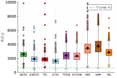
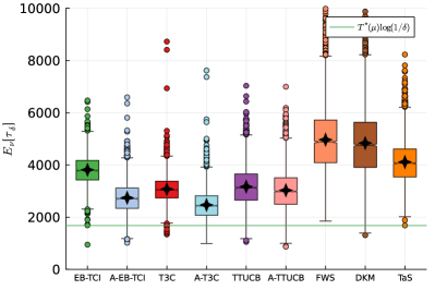
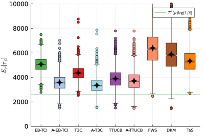
The ratio seems to reach its highest value for “equal means” instances (Lemma C.6), i.e. for all with . To best observe differences between Top Two algorithms with and their adaptive version, we consider such instances with (). Figure 6 reveals that adaptive proportions yield better empirical performance, with an empirical speed-up close to . We also compare them with three asymptotically optimal BAI algorithms (TaS, FWS and DKM). Even on those hard instances, Top Two algorithms with fixed are outperforming the asymptotically optimal algorithms for all the values . While being only asymptotically optimal, Top Two algorithms (with fixed ) can obtain significantly better empirical performances compared to existing asymptotically optimal in the finite-confidence regime. The gap between the empirical performance of the adaptive and the fixed Top Two algorithms is increasing with decreasing. Interestingly, TTUCB appears to be slightly more robust to decreasing confidence compared to other Top Two algorithms.
We also compare Top Two algorithms using a fixed proportion with their adaptive counterpart using at time on random instances.
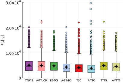
Experiments are conducted on random Gaussian instances with such that and for all . Figure 7 shows that their performances are highly similar, with a slim advantage for adaptive algorithms. For instances with multiple close competitors, the same phenomenon appears (see Figure 8 below). This is expected as is close to one when sub-optimal arms have significantly distinct means (see Figure 2).