Determination of spin-orbit interaction in semiconductor
nanostructures via non-linear transport
Abstract
We investigate non-linear transport signatures stemming from linear and cubic spin-orbit interactions in one- and two-dimensional systems. The analytical zero-temperature response to external fields is complemented by finite temperature numerical analysis, establishing a way to distinguish between linear and cubic spin-orbit interactions. We also propose a protocol to determine the relevant material parameters from transport measurements attainable in realistic conditions, illustrated by values for Ge heterostructures. Our results establish a method for the fast benchmarking of spin-orbit properties in semiconductor nanostructures.
Introduction - Engineering spin-orbit interactions (SOIs) in semiconductor nanostructures is a crucial challenge in several branches of physics, ranging from spintronics Žutić et al. (2004) and topological materials Laubscher and Klinovaja (2021); Hasan and Kane (2010); Armitage et al. (2018) to quantum information processing Hanson et al. (2007); Loss and DiVincenzo (1998); Kloeffel and Loss (2013). Notably, large values of SOIs emerge in nanowires Watzinger et al. (2018); Froning et al. (2021a, b); Wang et al. (2022a); Camenzind et al. (2022); Maurand et al. (2016); Crippa et al. (2018) and two-dimensional heterostructures Hendrickx et al. (2020a, b, 2021); Jirovec et al. (2022, 2021), where the charge carriers are holes in the valence band rather than electrons in the conduction band Winkler (2003). In these systems, the SOIs are also completely tunable by external electric fields Kloeffel et al. (2011, 2018); Adelsberger et al. (2022a, b); Gao et al. (2020); Venitucci et al. (2018); Michal et al. (2021); Bellentani et al. (2021), yielding sweet-spots against critical sources of noise Piot et al. (2022); Bosco et al. (2021a); Bosco and Loss (2022); Wang et al. (2021); Bosco and Loss (2021) and on-demand control of the interaction between qubits and resonators Yu et al. (2022); Kloeffel et al. (2013); Bosco et al. (2022); Michal et al. (2022); Mutter and Burkard (2020, 2021).
In particular, hole gases in planar germanium (Ge) heterostructures are emerging as highly promising candidates for processing quantum information Scappucci et al. (2021). Their large SOI enables ultrafast qubit operations at low power in a highly CMOS compatible platform Hendrickx et al. (2020a, b, 2021) and removes the need for additional bulky micromagnets Mi et al. (2018); Harvey-Collard et al. (2022); Watson et al. (2018); Takeda et al. (2020); Yoneda et al. (2020); Mills et al. (2022); Philips et al. (2022), offering a clear practical advantage for scaling up the next generation of quantum processors Vandersypen et al. (2017); Gonzalez-Zalba et al. (2021); Xue et al. (2021). Remarkably, in these structures, the SOI can be designed to be linear or cubic in momentum Bulaev and Loss (2007); Bosco et al. (2021b); Xiong et al. (2021); Terrazos et al. (2021); Wang et al. (2022b), greatly impacting the response of the material to external fields Gholizadeh and Culcer (2022). Despite its potential, an efficient and simple way to measure the SOI in these materials remains elusive.
From the early classification of solid-state systems in insulators, conductors, and semiconductors Ashcroft and Mermin (1976) to the more recent discovery of the role of geometry and topology in non-trivial band structures Xiao et al. (2010); Hasan and Kane (2010); Armitage et al. (2018); Lv et al. (2021), transport experiments have been at the core of condensed matter physics, providing arguably the most practical yet insightful way to probe the physics of solid-state systems. While most of the seminal effects, such as the integer quantum Hall Klitzing et al. (1980); Laughlin (1981); Thouless et al. (1982); Haldane (1988) or the anomalous Hall Nagaosa et al. (2010); Chang et al. (2013); Nakatsuji et al. (2015); Yasuda et al. (2016); Liu et al. (2018) effect, depend linearly on the external fields, lately, an increasing number of novel transport properties in materials with non-trivial band structure have been reported in the non-linear regime Oka and Aoki (2009); Son and Spivak (2013); Sodemann and Fu (2015); Morimoto and Nagaosa (2016); de Juan et al. (2017); Tokura and Nagaosa (2018); Ma et al. (2019); Kang et al. (2019); Kovalev et al. (2020); Dantas et al. (2021); Morimoto and Nagaosa (2016); Kawabata and Ueda (2021); Matus et al. (2022); Legg et al. (2022a); Germanskiy et al. (2022). A particularly fruitful direction has been the application of dc non-linear responses, such as magnetochiral anisotropy (also known as bilinear magnetoresistance) and non-linear Hall effects, to gain insight into the electronic structure of the system Ideue et al. (2017); He et al. (2018, 2019); Vaz et al. (2020); Legg et al. (2022b); Wang et al. (2022c, d, e, f).
In this work, we employ Boltzmann transport theory to study the response of one- (1D) and two-dimensional (2D) nanostructures with linear and cubic SOI and show that these effects leave distinct signatures in the non-linear response of the system. Moreover, numerical analyses for realistic material parameters and small finite temperatures support the zero-temperature analytics and confirm that these signatures can be measured in state-of-the-art experiments. This work paves the way for a functional and time-efficient experimental characterization of SOI in these semiconductor nanostructures, enabling fast benchmarking already at the material level.
1D -
First, we consider 1D systems, e.g. nanowires, described by the effective Hamiltonian Hetényi et al. (2022)
| (1) |
where we assume Einstein summation convention, and , resp., correspond to SOI linear and cubic in momentum , is the effective mass, are the elements of the Pauli vector acting in (pseudo-) spin space, and (no summation implied) is the Zeeman field, written in terms of the components of the diagonal -tensor and the external magnetic field 111Note that the Hamiltonian of Eq. (1) is an effective description only valid for small chemicals potentials and momenta.. The cubic SOI is often neglected but it can yield significant anisotropies in the spectrum of quantum dots Katsaros et al. (2020); Hetényi et al. (2022) and, as we shall see, can be determined via transport measurements. The energy dispersion for such a two-band Hamiltonian is given by
| (2) |
The response of the system to a static external electric field, aligned with the nanowire axis (), is obtained by solving perturbatively the Boltzmann equation within the relaxation time approximation
| (3) |
where is the out-of-equilibrium distribution for the band, is the Fermi-Dirac distribution, and is the intra-band relaxation time. In 1D, the dynamics of holes are governed solely by the electric field, i.e. , where is the elementary charge. The current density can be written as a power series in the electric field , which at zero temperature, , is given by
| (4) |
where , is the group velocity, and is the Fermi wave vector associated with the band [obtained from ] Ideue et al. (2017); Morimoto and Nagaosa (2016); Legg et al. (2022b).
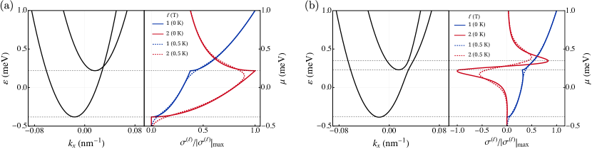
To gain insight into the impact of the SOI, we first consider aligned with the spin polarization axis of the system. Due to the SOI, the otherwise degenerate quadratic bands develop a finite spin expectation value along the -direction and, in the presence of a collinear magnetic field , become spin-split []. In this case, the only non-zero contribution in Eq. (4), aside from the linear term, which is dominated by the kinetic term and hence less useful to extract information about SOI, is given by the term quadratic in ,
| (5) |
where is the positive (negative) Fermi wave vector associated with the band . Note that is directly proportional to the cubic SOI coupling , providing a way to directly determine the presence of this effect from the second-order conductivity , defined by . Alternatively, non-linear currents can be induced in systems lacking cubic SOI by choosing such that (Fig. 1) Legg et al. (2022a).
2D - We now consider the effect of linear and cubic SOI in a 2D system described by the effective Hamiltonian
| (6) |
where and . Here, , , and are the linear, isotropic cubic, and anisotropic cubic SOI constants, resp. Bulaev and Loss (2005, 2007); Marcellina et al. (2017); Miserev and Sushkov (2017); Terrazos et al. (2021); Luethi et al. (2022). The energy dispersion reads
| (7) |
where
To set the parameter values, hereafter we consider Ge [100] and [110] for realistic experimental conditions. While both systems have similar effective masses and cubic SOIs, assumed as , and , they differ in the linear SOI, which is absent for Ge [100] and takes the value for Ge [110] Xiong et al. (2021). Further, for Ge [100], while for Ge [110], .
Compared to 1D, the dynamics of the hole quasiparticles is not only enriched by orbital effects for out-of-plane magnetic fields but also by the band geometry, captured by the equations of motion
| (8) |
where is the Berry curvature, with , and is the group velocity for the dispersion modified by the orbital magnetic moment of the wave packet, Xiao et al. (2010). Note that, because we consider holes, the quasimomentum couples with opposite sign to the electric field when compared to the case of electrons. Since for 2D systems both and are perpendicular to the plane, we can greatly simplify the problem by restricting to in-plane fields, . This suffices to determine both SOI and in-plane -factors. This simplification renders the physics similar to 1D, allowing the result from Eq. (4) to be generalized, such that the -order contribution to the current becomes
| (9) |
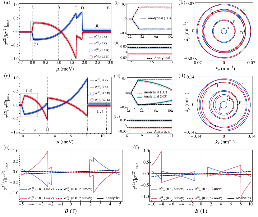
where denotes the line integral over the Fermi surface (FS), , and . This expression can be used to numerically access the response at . Henceforth, we focus on the lowest order non-linear response impacted by the SOI and study the order conductivities , defined by . Importantly, second order conductivities correspond to a rectification of current and are genereally only allowed in the presence of both broken inversion symmetry and time reversal symmetry (see below), this makes them highly sensitive to the presence of SOI Ideue et al. (2017); He et al. (2018, 2019); Legg et al. (2022b); Wang et al. (2022c). We use Eq. (9) to compute longitudinal, , and tranversal, , conductivities for Ge[100] and [110] for T, see Figs. 2(a,c).
Since for in-plane magnetic fields linear and non-linear conductivities are solely connected to the energy dispersion [Eq. (9)], these quantities reflect the competition between the kinetic, Zeeman, and SOI energies. We identify three different regimes from the conductivities [Fig. 2(a) and (c)] which can be used to fully determine the SOI and in-plane -factors. At small chemical potentials , the energy associated with SOI sets the smallest energy scale in the problem, allowing for the analytical computation of the conductivities. To linear order in SOI and for a generic in-plane magnetic field, we find
| (10) | |||||
| (11) |
and , , with
| (12) |
, and . The comparison between these expressions and the numerical results obtained with Eq. (9) are presented in Figs. 2(a.i) and 2(c.iii). As increases, the SOI becomes more significant and higher-order terms in the SOI need to be included [see Fig. 2(c.iii) for comparison of linear and higher-order analytical results]. Although full analytical treatment is possible, the expressions are too lengthy to be shown here.
The second regime emerges when the SOI becomes comparable to the Zeeman energy . This regime is delimited by the Fermi energies where the two Fermi contours touch each other [see contours C and D in Fig. 2(b) and contours H and I in Fig. 2(d)], leading to a discontinuity in the order conductivities [Figs. 2(a) and 2(c)]. For beyond this point, the response can be computed perturbatively in ,
| (13) | ||||
| (14) |
and . Here, we have neglected the linear SOI and assume that . Yet, these expressions describe extremely well the numerical results based on Eq. (9) even for systems with small linear SOI, see Figs. 2(a.ii) and 2(c.iv).
It is important to note that the expressions in Eqs. (10-14) do not depend on the linear SOI. Nevertheless, the amplitude of the linear SOI can be inferred from the position of the discontinuities in the second-order conductivities, which for in -direction are given by 222Note that without linear SOI, corresponding to Ge [100], the discontinuities in occur at and .
| (15) |
with
| (16) |
and . This information can also be inferred by varying instead of , see Figs. 2(e) and 2(f).
Experimental realization - The conductivities are straightforwardly related to the experimentally measured second-order resistivities , defined by , via Lahiri et al. (2022)
| (17) |
Here, represents the inverse matrix of the first-order conductivity tensor, which is well described by
| (18) |
In Fig. 3 we show the evaluation of for Ge[100] and Ge[110]. We note that can be obtained from standard transport experiments by measuring the second-harmonic component of the voltage induced by an ac 333Here, the frequency of the ac current is chosen such that . This way, the high-harmonics probe only the dc properties of the system and contain no information about the dynamical response of the system to the oscillatory driving perturbation Kovalev et al. (2020); Dantas et al. (2021); Wang et al. (2022c); Germanskiy et al. (2022). current Ideue et al. (2017); Tokura and Nagaosa (2018); He et al. (2018, 2019); Legg et al. (2022b).
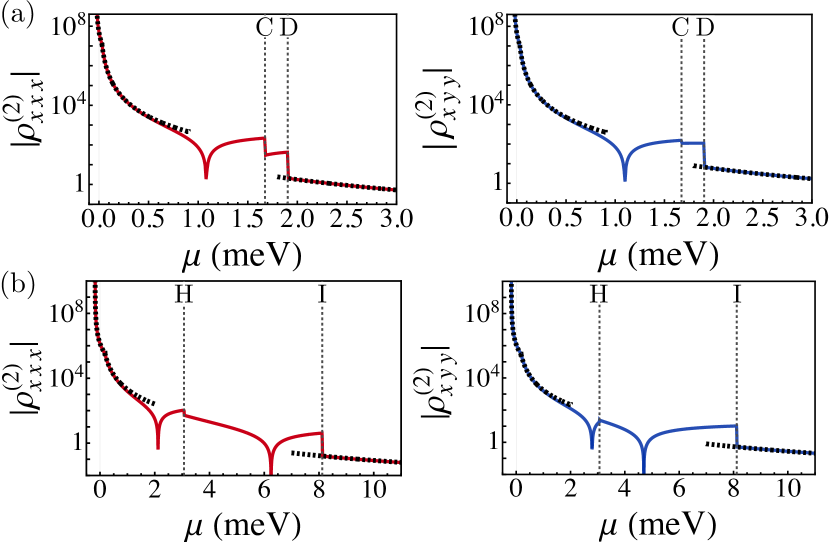
Finally, we address the extraction of the SOI couplings and in-plane -factors for a 2D system. As shown in Fig. 3, Eqs. (10-14) and (17-18) provide a good fit to the numerical results for and . Consequently, cubic SOI can be inferred from the measurement of the first- and second-order resistivity (or resistance) tensor in any of these regimes. Note, however, that, although the non-linear resistivity is smaller for , this regime has the advantage of not requiring strong in-plane magnetic fields and being more robust to temperature fluctuations. Moreover, kinetic theory is most adequate to model the transport properties of the system in this regime, as the effect of disorder is less pronounced. Lastly, we remark again that the linear SOI coupling and the in-plane -factors can then be extracted from the position of the discontinuitites in the resistivity, using Eqs. (15-16).
Conclusion - We discussed the effect of linear and cubic SOIs on the transport properties of 1D and 2D systems with large SOI and how non-linear responses can be used to characterize this effect with standard transport measurements. In nanowires, we demonstrated that the cubic SOI induces a non-linear response current quadratic in the electric field [Eq. (5)] when the system is subjected to an external magnetic field aligned with the spin polarization axis [Fig. 1(a)]. Moreover, the linear SOI was shown to contribute to this non-linear current for noncollinear configurations of magnetic field and SOI direction, substantiating the use of the second-order conductivity to extract both and [Fig. 1(b)]. Linear and cubic SOI were also proven to leave their imprint on the non-linear response of 2D systems in the presence of in-plane magnetic fields. More specifically, we showed that both longitudinal [ and ] and transversal [ and ] second-order conductivities can be used to determined not only the SOI couplings, but also the in-plane -factors of the system [Eqs. (10-14)]. Numerical results for finite temperatures and realistic material parameters substantiate our zero-temperature analytical findings, establishing an operative characterization of the SOI and in-plane -factors from measurements of non-linear resistivities in simple transport experiments.
Acknowledgements.
Acknowledgements - This work was supported by the Georg H. Endress Foundation and as a part of NCCR SPIN funded by the Swiss National Science Foundation (grant no. 51NF40-180604). This project received funding from the European Union’s Horizon 2020 research and innovation program (ERC Starting Grant, grant agreement No. 757725).References
- Žutić et al. (2004) I. Žutić, J. Fabian, and S. Das Sarma, Rev. Mod. Phys. 76, 323 (2004).
- Laubscher and Klinovaja (2021) K. Laubscher and J. Klinovaja, Journal of Applied Physics 130, 081101 (2021).
- Hasan and Kane (2010) M. Z. Hasan and C. L. Kane, Rev. Mod. Phys. 82, 3045 (2010).
- Armitage et al. (2018) N. P. Armitage, E. J. Mele, and A. Vishwanath, Rev. Mod. Phys. 90, 015001 (2018).
- Hanson et al. (2007) R. Hanson, L. P. Kouwenhoven, J. R. Petta, S. Tarucha, and L. M. K. Vandersypen, Rev. Mod. Phys. 79, 1217 (2007).
- Loss and DiVincenzo (1998) D. Loss and D. P. DiVincenzo, Phys. Rev. A 57, 120 (1998).
- Kloeffel and Loss (2013) C. Kloeffel and D. Loss, Annual Review of Condensed Matter Physics 4, 51 (2013).
- Watzinger et al. (2018) H. Watzinger, J. Kukučka, L. Vukušić, F. Gao, T. Wang, F. Schäffler, J.-J. Zhang, and G. Katsaros, Nature Communications 9, 3902 (2018).
- Froning et al. (2021a) F. N. M. Froning, L. C. Camenzind, O. A. H. van der Molen, A. Li, E. P. A. M. Bakkers, D. M. Zumbühl, and F. R. Braakman, Nature Nanotechnology 16, 308 (2021a).
- Froning et al. (2021b) F. N. M. Froning, M. J. Rančić, B. Hetényi, S. Bosco, M. K. Rehmann, A. Li, E. P. A. M. Bakkers, F. A. Zwanenburg, D. Loss, D. M. Zumbühl, and F. R. Braakman, Phys. Rev. Research 3, 013081 (2021b).
- Wang et al. (2022a) K. Wang, G. Xu, F. Gao, H. Liu, R.-L. Ma, X. Zhang, Z. Wang, G. Cao, T. Wang, J.-J. Zhang, D. Culcer, X. Hu, H.-W. Jiang, H.-O. Li, G.-C. Guo, and G.-P. Guo, Nature Communications 13, 206 (2022a).
- Camenzind et al. (2022) L. C. Camenzind, S. Geyer, A. Fuhrer, R. J. Warburton, D. M. Zumbühl, and A. V. Kuhlmann, Nature Electronics 5, 178 (2022).
- Maurand et al. (2016) R. Maurand, X. Jehl, D. Kotekar-Patil, A. Corna, H. Bohuslavskyi, R. Laviéville, L. Hutin, S. Barraud, M. Vinet, M. Sanquer, and S. De Franceschi, Nature communications 7, 1 (2016).
- Crippa et al. (2018) A. Crippa, R. Maurand, L. Bourdet, D. Kotekar-Patil, A. Amisse, X. Jehl, M. Sanquer, R. Laviéville, H. Bohuslavskyi, L. Hutin, S. Barraud, M. Vinet, Y.-M. Niquet, and S. De Franceschi, Phys. Rev. Lett. 120, 137702 (2018).
- Hendrickx et al. (2020a) N. W. Hendrickx, W. I. L. Lawrie, L. Petit, A. Sammak, G. Scappucci, and M. Veldhorst, Nature Communications 11, 3478 (2020a).
- Hendrickx et al. (2020b) N. Hendrickx, D. Franke, A. Sammak, G. Scappucci, and M. Veldhorst, Nature 577, 487 (2020b).
- Hendrickx et al. (2021) N. W. Hendrickx, W. I. L. Lawrie, M. Russ, F. van Riggelen, S. L. de Snoo, R. N. Schouten, A. Sammak, G. Scappucci, and M. Veldhorst, Nature 591, 580 (2021).
- Jirovec et al. (2022) D. Jirovec, P. M. Mutter, A. Hofmann, A. Crippa, M. Rychetsky, D. L. Craig, J. Kukucka, F. Martins, A. Ballabio, N. Ares, D. Chrastina, G. Isella, G. Burkard, and G. Katsaros, Phys. Rev. Lett. 128, 126803 (2022).
- Jirovec et al. (2021) D. Jirovec, A. Hofmann, A. Ballabio, P. M. Mutter, G. Tavani, M. Botifoll, A. Crippa, J. Kukucka, O. Sagi, F. Martins, J. Saez-Mollejo, I. Prieto, M. Borovkov, J. Arbiol, D. Chrastina, G. Isella, and G. Katsaros, Nature Materials 20, 1106 (2021).
- Winkler (2003) R. Winkler, Spin–Orbit Coupling Effects in Two-Dimensional Electron and Hole Systems, edited by G. Höhler, J. H. Kühn, T. Müller, J. Trümper, A. Ruckenstein, P. Wölfle, and F. Steiner, Springer Tracts in Modern Physics, Vol. 191 (Springer Berlin Heidelberg, Berlin, Heidelberg, 2003).
- Kloeffel et al. (2011) C. Kloeffel, M. Trif, and D. Loss, Phys. Rev. B 84, 195314 (2011).
- Kloeffel et al. (2018) C. Kloeffel, M. J. Rančić, and D. Loss, Phys. Rev. B 97, 235422 (2018).
- Adelsberger et al. (2022a) C. Adelsberger, M. Benito, S. Bosco, J. Klinovaja, and D. Loss, Phys. Rev. B 105, 075308 (2022a).
- Adelsberger et al. (2022b) C. Adelsberger, S. Bosco, J. Klinovaja, and D. Loss, arXiv:2207.12050 (2022b).
- Gao et al. (2020) F. Gao, J.-H. Wang, H. Watzinger, H. Hu, M. J. Rančić, J.-Y. Zhang, T. Wang, Y. Yao, G.-L. Wang, J. Kukučka, L. Vukušić, C. Kloeffel, D. Loss, F. Liu, G. Katsaros, and J.-J. Zhang, Advanced Materials 32, 1906523 (2020).
- Venitucci et al. (2018) B. Venitucci, L. Bourdet, D. Pouzada, and Y.-M. Niquet, Phys. Rev. B 98, 155319 (2018).
- Michal et al. (2021) V. P. Michal, B. Venitucci, and Y.-M. Niquet, Phys. Rev. B 103, 045305 (2021).
- Bellentani et al. (2021) L. Bellentani, M. Bina, S. Bonen, A. Secchi, A. Bertoni, S. P. Voinigescu, A. Padovani, L. Larcher, and F. Troiani, Phys. Rev. Applied 16, 054034 (2021).
- Piot et al. (2022) N. Piot, B. Brun, V. Schmitt, S. Zihlmann, V. P. Michal, A. Apra, J. C. Abadillo-Uriel, X. Jehl, B. Bertrand, H. Niebojewski, L. Hutin, M. Vinet, M. Urdampilleta, T. Meunier, Y. M. Niquet, R. Maurand, and S. D. Franceschi, Nature Nanotechnology (2022).
- Bosco et al. (2021a) S. Bosco, B. Hetényi, and D. Loss, PRX Quantum 2, 010348 (2021a).
- Bosco and Loss (2022) S. Bosco and D. Loss, arXiv:2204.08212 (2022).
- Wang et al. (2021) Z. Wang, E. Marcellina, A. R. Hamilton, J. H. Cullen, S. Rogge, J. Salfi, and D. Culcer, npj Quantum Information 7, 54 (2021).
- Bosco and Loss (2021) S. Bosco and D. Loss, Phys. Rev. Lett. 127, 190501 (2021).
- Yu et al. (2022) C. X. Yu, S. Zihlmann, J. C. Abadillo-Uriel, V. P. Michal, N. Rambal, H. Niebojewski, T. Bedecarrats, M. Vinet, E. Dumur, M. Filippone, B. Bertrand, S. De Franceschi, Y.-M. Niquet, and R. Maurand, arXiv:2206.14082 (2022).
- Kloeffel et al. (2013) C. Kloeffel, M. Trif, P. Stano, and D. Loss, Phys. Rev. B 88, 241405 (2013).
- Bosco et al. (2022) S. Bosco, P. Scarlino, J. Klinovaja, and D. Loss, Phys. Rev. Lett. 129, 066801 (2022).
- Michal et al. (2022) V. Michal, J. Abadillo-Uriel, S. Zihlmann, R. Maurand, Y.-M. Niquet, and M. Filippone, arXiv:2204.00404 (2022).
- Mutter and Burkard (2020) P. M. Mutter and G. Burkard, Phys. Rev. B 102, 205412 (2020).
- Mutter and Burkard (2021) P. M. Mutter and G. Burkard, Phys. Rev. Research 3, 013194 (2021).
- Scappucci et al. (2021) G. Scappucci, C. Kloeffel, F. A. Zwanenburg, D. Loss, M. Myronov, J.-J. Zhang, S. De Franceschi, G. Katsaros, and M. Veldhorst, Nature Reviews Materials 6, 926 (2021).
- Mi et al. (2018) X. Mi, M. Benito, S. Putz, D. M. Zajac, J. M. Taylor, G. Burkard, and J. R. Petta, Nature 555, 599 (2018).
- Harvey-Collard et al. (2022) P. Harvey-Collard, J. Dijkema, G. Zheng, A. Sammak, G. Scappucci, and L. M. K. Vandersypen, Phys. Rev. X 12, 021026 (2022).
- Watson et al. (2018) T. F. Watson, S. G. J. Philips, E. Kawakami, D. R. Ward, P. Scarlino, M. Veldhorst, D. E. Savage, M. G. Lagally, M. Friesen, S. N. Coppersmith, M. A. Eriksson, and L. M. K. Vandersypen, Nature 555, 633 (2018).
- Takeda et al. (2020) K. Takeda, A. Noiri, J. Yoneda, T. Nakajima, and S. Tarucha, Phys. Rev. Lett. 124, 117701 (2020).
- Yoneda et al. (2020) J. Yoneda, K. Takeda, A. Noiri, T. Nakajima, S. Li, J. Kamioka, T. Kodera, and S. Tarucha, Nature Communications 11, 1144 (2020).
- Mills et al. (2022) A. R. Mills, C. R. Guinn, M. J. Gullans, A. J. Sigillito, M. M. Feldman, E. Nielsen, and J. R. Petta, Science Advances 8, eabn5130 (2022).
- Philips et al. (2022) S. G. Philips, M. T. Madzik, S. V. Amitonov, S. L. de Snoo, M. Russ, N. Kalhor, C. Volk, W. I. Lawrie, D. Brousse, L. Tryputen, B. P. Wuetz, A. Sammak, M. Veldhorst, G. Scappucci, and L. M. Vandersypen, arXiv:2202.09252 (2022).
- Vandersypen et al. (2017) L. M. K. Vandersypen, H. Bluhm, J. S. Clarke, A. S. Dzurak, R. Ishihara, A. Morello, D. J. Reilly, L. R. Schreiber, and M. Veldhorst, Npj Quantum Inf. 3, 1 (2017).
- Gonzalez-Zalba et al. (2021) M. F. Gonzalez-Zalba, S. de Franceschi, E. Charbon, T. Meunier, M. Vinet, and A. S. Dzurak, Nature Electronics 4, 872 (2021).
- Xue et al. (2021) X. Xue, B. Patra, J. P. G. van Dijk, N. Samkharadze, S. Subramanian, A. Corna, B. Paquelet Wuetz, C. Jeon, F. Sheikh, E. Juarez-Hernandez, B. P. Esparza, H. Rampurawala, B. Carlton, S. Ravikumar, C. Nieva, S. Kim, H.-J. Lee, A. Sammak, G. Scappucci, M. Veldhorst, F. Sebastiano, M. Babaie, S. Pellerano, E. Charbon, and L. M. K. Vandersypen, Nature 593, 205 (2021).
- Bulaev and Loss (2007) D. V. Bulaev and D. Loss, Phys. Rev. Lett. 98, 097202 (2007).
- Bosco et al. (2021b) S. Bosco, M. Benito, C. Adelsberger, and D. Loss, Phys. Rev. B 104, 115425 (2021b).
- Xiong et al. (2021) J.-X. Xiong, S. Guan, J.-W. Luo, and S.-S. Li, Phys. Rev. B 103, 085309 (2021).
- Terrazos et al. (2021) L. A. Terrazos, E. Marcellina, Z. Wang, S. N. Coppersmith, M. Friesen, A. R. Hamilton, X. Hu, B. Koiller, A. L. Saraiva, D. Culcer, and R. B. Capaz, Phys. Rev. B 103, 125201 (2021).
- Wang et al. (2022b) C.-A. Wang, G. Scappucci, M. Veldhorst, and M. Russ, arXiv:2208.04795 (2022b).
- Gholizadeh and Culcer (2022) S. Gholizadeh and D. Culcer, arXiv:2206.11916 (2022).
- Ashcroft and Mermin (1976) N. W. Ashcroft and N. D. Mermin, Solid State Physics (Holt-Saunders, 1976).
- Xiao et al. (2010) D. Xiao, M.-C. Chang, and Q. Niu, Rev. Mod. Phys. 82, 1959 (2010).
- Lv et al. (2021) B. Q. Lv, T. Qian, and H. Ding, Rev. Mod. Phys. 93, 025002 (2021).
- Klitzing et al. (1980) K. v. Klitzing, G. Dorda, and M. Pepper, Phys. Rev. Lett. 45, 494 (1980).
- Laughlin (1981) R. B. Laughlin, Phys. Rev. B 23, 5632 (1981).
- Thouless et al. (1982) D. J. Thouless, M. Kohmoto, M. P. Nightingale, and M. den Nijs, Phys. Rev. Lett. 49, 405 (1982).
- Haldane (1988) F. D. M. Haldane, Phys. Rev. Lett. 61, 2015 (1988).
- Nagaosa et al. (2010) N. Nagaosa, J. Sinova, S. Onoda, A. H. MacDonald, and N. P. Ong, Rev. Mod. Phys. 82, 1539 (2010).
- Chang et al. (2013) C.-Z. Chang, J. Zhang, X. Feng, J. Shen, Z. Zhang, M. Guo, K. Li, Y. Ou, P. Wei, L.-L. Wang, Z.-Q. Ji, Y. Feng, S. Ji, X. Chen, J. Jia, X. Dai, Z. Fang, S.-C. Zhang, K. He, Y. Wang, L. Lu, X.-C. Ma, and Q.-K. Xue, Science 340, 167 (2013).
- Nakatsuji et al. (2015) S. Nakatsuji, N. Kiyohara, and T. Higo, Nature 527, 212 (2015).
- Yasuda et al. (2016) K. Yasuda, R. Wakatsuki, T. Morimoto, R. Yoshimi, A. Tsukazaki, K. S. Takahashi, M. Ezawa, M. Kawasaki, N. Nagaosa, and Y. Tokura, Nature Physics 12, 555 (2016).
- Liu et al. (2018) E. Liu, Y. Sun, N. Kumar, L. Muechler, A. Sun, L. Jiao, S.-Y. Yang, D. Liu, A. Liang, Q. Xu, J. Kroder, V. Süß, H. Borrmann, C. Shekhar, Z. Wang, C. Xi, W. Wang, W. Schnelle, S. Wirth, Y. Chen, S. T. B. Goennenwein, and C. Felser, Nature Physics 14, 1125 (2018).
- Oka and Aoki (2009) T. Oka and H. Aoki, Phys. Rev. B 79, 081406 (2009).
- Son and Spivak (2013) D. T. Son and B. Z. Spivak, Phys. Rev. B 88, 104412 (2013).
- Sodemann and Fu (2015) I. Sodemann and L. Fu, Phys. Rev. Lett. 115, 216806 (2015).
- Morimoto and Nagaosa (2016) T. Morimoto and N. Nagaosa, Phys. Rev. Lett. 117, 146603 (2016).
- de Juan et al. (2017) F. de Juan, A. G. Grushin, T. Morimoto, and J. E. Moore, Nature Communications 8, 15995 (2017).
- Tokura and Nagaosa (2018) Y. Tokura and N. Nagaosa, Nature Communications 9, 3740 (2018).
- Ma et al. (2019) Q. Ma, S.-Y. Xu, H. Shen, D. MacNeill, V. Fatemi, T.-R. Chang, A. M. Mier Valdivia, S. Wu, Z. Du, C.-H. Hsu, S. Fang, Q. D. Gibson, K. Watanabe, T. Taniguchi, R. J. Cava, E. Kaxiras, H.-Z. Lu, H. Lin, L. Fu, N. Gedik, and P. Jarillo-Herrero, Nature 565, 337 (2019).
- Kang et al. (2019) K. Kang, T. Li, E. Sohn, J. Shan, and K. F. Mak, Nature Materials 18, 324 (2019).
- Kovalev et al. (2020) S. Kovalev, R. M. A. Dantas, S. Germanskiy, J.-C. Deinert, B. Green, I. Ilyakov, N. Awari, M. Chen, M. Bawatna, J. Ling, F. Xiu, P. H. M. van Loosdrecht, P. Surówka, T. Oka, and Z. Wang, Nature Communications 11, 2451 (2020).
- Dantas et al. (2021) R. M. A. Dantas, Z. Wang, P. Surówka, and T. Oka, Phys. Rev. B 103, L201105 (2021).
- Kawabata and Ueda (2021) K. Kawabata and M. Ueda, arXiv:2110.08304 (2021).
- Matus et al. (2022) P. Matus, R. M. A. Dantas, R. Moessner, and P. Surówka, Proceedings of the National Academy of Sciences 119, e2200367119 (2022).
- Legg et al. (2022a) H. F. Legg, D. Loss, and J. Klinovaja, Phys. Rev. B 106, 104501 (2022a).
- Germanskiy et al. (2022) S. Germanskiy, R. M. A. Dantas, S. Kovalev, C. Reinhoffer, E. A. Mashkovich, P. H. M. van Loosdrecht, Y. Yang, F. Xiu, P. Surówka, R. Moessner, T. Oka, and Z. Wang, Phys. Rev. B 106, L081127 (2022).
- Ideue et al. (2017) T. Ideue, K. Hamamoto, S. Koshikawa, M. Ezawa, S. Shimizu, Y. Kaneko, Y. Tokura, N. Nagaosa, and Y. Iwasa, Nature Physics 13, 578 (2017).
- He et al. (2018) P. He, S. S. L. Zhang, D. Zhu, Y. Liu, Y. Wang, J. Yu, G. Vignale, and H. Yang, Nature Physics 14, 495 (2018).
- He et al. (2019) P. He, S. S.-L. Zhang, D. Zhu, S. Shi, O. G. Heinonen, G. Vignale, and H. Yang, Phys. Rev. Lett. 123, 016801 (2019).
- Vaz et al. (2020) D. C. Vaz, F. Trier, A. Dyrdał, A. Johansson, K. Garcia, A. Barthélémy, I. Mertig, J. Barnaś, A. Fert, and M. Bibes, Phys. Rev. Materials 4, 071001 (2020).
- Legg et al. (2022b) H. F. Legg, M. Rößler, F. Münning, D. Fan, O. Breunig, A. Bliesener, G. Lippertz, A. Uday, A. A. Taskin, D. Loss, J. Klinovaja, and Y. Ando, Nature Nanotechnology 17, 696 (2022b).
- Wang et al. (2022c) Y. Wang, H. F. Legg, T. Bömerich, J. Park, S. Biesenkamp, A. A. Taskin, M. Braden, A. Rosch, and Y. Ando, Phys. Rev. Lett. 128, 176602 (2022c).
- Wang et al. (2022d) Y. Wang, S. V. Mambakkam, Y.-X. Huang, Y. Wang, Y. Ji, C. Xiao, S. A. Yang, S. A. Law, and J. Q. Xiao, arXiv:2203.06293 (2022d).
- Wang et al. (2022e) Y. Wang, T. Boemerich, J. Park, H. F. Legg, A. A. Taskin, A. Rosch, and Y. Ando, arXiv:2208.10314 (2022e).
- Wang et al. (2022f) Y. Wang, B. Liu, Y.-X. Huang, S. V. Mambakkam, Y. Wang, S. A. Yang, X.-L. Sheng, S. A. Law, and J. Q. Xiao, arXiv:2209.07666 (2022f).
- Hetényi et al. (2022) B. Hetényi, S. Bosco, and D. Loss, Phys. Rev. Lett. 129, 116805 (2022).
- Note (1) Note that the Hamiltonian of Eq. (1) is an effective description only valid for small chemicals potentials and momenta.
- Katsaros et al. (2020) G. Katsaros, J. Kukučka, L. Vukušić, H. Watzinger, F. Gao, T. Wang, J.-J. Zhang, and K. Held, Nano Letters 20, 5201 (2020).
- Bulaev and Loss (2005) D. V. Bulaev and D. Loss, Phys. Rev. Lett. 95, 076805 (2005).
- Marcellina et al. (2017) E. Marcellina, A. R. Hamilton, R. Winkler, and D. Culcer, Phys. Rev. B 95, 075305 (2017).
- Miserev and Sushkov (2017) D. S. Miserev and O. P. Sushkov, Phys. Rev. B 95, 085431 (2017).
- Luethi et al. (2022) M. Luethi, K. Laubscher, S. Bosco, D. Loss, and J. Klinovaja, arXiv:2209.12745 (2022).
- Lodari et al. (2022) M. Lodari, O. Kong, M. Rendell, A. Tosato, A. Sammak, M. Veldhorst, A. R. Hamilton, and G. Scappucci, Applied Physics Letters 120, 122104 (2022).
- Note (2) Note that without linear SOI, corresponding to Ge [100], the discontinuities in occur at and .
- Lahiri et al. (2022) S. Lahiri, T. Bhore, K. Das, and A. Agarwal, Phys. Rev. B 105, 045421 (2022).
- Note (3) Here, the frequency of the ac current is chosen such that . This way, the high-harmonics probe only the dc properties of the system and contain no information about the dynamical response of the system to the oscillatory driving perturbation Kovalev et al. (2020); Dantas et al. (2021); Wang et al. (2022c); Germanskiy et al. (2022).