Modeling photometric variations due to a global inhomogeneity on an obliquely rotating star: application to lightcurves of white dwarfs

Abstract

We develop a general framework to compute photometric variations induced by the oblique rotation of a star with an axisymmetric inhomogeneous surface. We apply the framework to compute lightcurves of white dwarfs adopting two simple models of their surface inhomogeneity. Depending on the surface model and the location of the observer, the resulting lightcurve exhibits a departure from a purely sinusoidal curve that are observed for a fraction of white dwarfs. As a specific example, we fit our model to the observed phase-folded lightcurve of a fast-spinning white dwarf ZTF J190132.9+145808.7 (with the rotation period of 419s). We find that the size and obliquity angle of the spot responsible for the photometric variation are $\Delta\theta_{\rm s}\approx 60^{\circ}$ and $\theta_{\star}\approx 60^{\circ}$ or $90^{\circ}$, respectively, implying an interesting constraint on the surface distribution of the magnetic field on white dwarfs.

1 Introduction

A number of white dwarfs (WDs) have exhibited periodic photometric variations (e.g., Achilleos et al., 1992; Barstow et al., 1995; Wade et al., 2003; Brinkworth et al., 2005, 2013; Reding et al., 2020; Caiazzo et al., 2021; Kilic et al., 2021; Williams et al., 2022). Those variations are commonly interpreted to originate from inhomogeneities on the stellar surface that obliquely rotate around the spin axis. Those inhomogeneities may be produced by magnetic spots in a convective atmosphere (e.g., Valyavin et al., 2008, 2011) or the so-called magnetic dichroism (Ferrario et al., 1997); the continuum opacity changes with rotational phase according to the amplitude of the magnetic field strength across the stellar disk. As a result, the photometric flux varies as well. Hence, photometric lightcurves of WDs carry rich information on the distribution of the surface magnetic fields, which may be further disentangled by combining the spectro-polarimetric data if available (e.g., Liebert et al., 1977; Donati et al., 1994; Euchner et al., 2002; Valyavin et al., 2014).

For instance, Brinkworth et al. (2013) have performed time-series photometry of 30 isolated magnetic WDs, and 5 (24 %) are variable with reliably measured periods of (1 – 7) hours. Quite interestingly, all of their lightcurves are well fitted by a monochromatic sinusoidal curve. Indeed, apart from 9 WDs whose lightcurves are significantly contaminated by their varying comparison stars, they find that 14 out of the remaining 21 show evidence for variability whose lightcurves are consistent with a monochromatic sinusoidal curve. In marked contrast to other stars for which non-sinusoidal rotation signatures are commonly observed (e.g., Roettenbacher et al., 2013), the sinusoidal lightcurve seems to be fairly generic for these types of WDs, which have a relatively stable surface structure over time.

Thanks to the Kepler satellite, Transiting Exoplanet Survey Satellite (TESS), and Zwicky Transient Facility (ZTF) (Maoz et al., 2015; Reding et al., 2020; Hermes et al., 2021) among others, the number of photometric lightcurves for WDs with a high accuracy and cadence is rapidly increasing. Indeed, fast-spinning WDs with a rotation period even less than 10 minutes have been recently discovered (Reding et al., 2020; Caiazzo et al., 2021; Kilic et al., 2021). For such cases, however, it may be due to their pulsation, instead of the rotation, since their frequency ranges are overlapped (e.g., Winget & Kepler, 2008; Hollands et al., 2020). This points to an importance of quantitative modeling of photometric lightcurves due to inhomogeneities on rotating stars. For instance, the phase-folded lightcurve of one of the fast-spinning WDs (ZTF J190132.9+145808.7) seems to exhibit a non-sinusoidal feature (Caiazzo et al., 2021, and see Sec. 3.5 below), which could be relatively common for these young massive WDs. Thus, such modeling of photometric variations due to an inhomogeneity on the stellar surface should become even more crucial in the coming era of the Rubin Observatory LSST Camera (Ivezić et al., 2019).

Photometric rotational variations due to multiple circular starspots have been studied previously (e.g., Budding, 1977; Dorren, 1987; Eker, 1994; Landolfi et al., 1997; Kipping, 2012). More recently, Suto et al. (2022) proposed a fully analytic model for the photometric variations due to infinitesimally small multiple starspots on a differentially rotating star, and performed a series of mock Lomb-Scargle analysis relevant to the Kepler data (e.g., Lu et al., 2022). In this paper, instead, we focus on an inhomogeneous surface intensity pattern that is axisymmetric around an axis misaligned to the stellar spin axis. The inhomogeneity produces periodic photometric variations due to the stellar rotation. The purpose of the present paper is to develop a general formulation to describe the rotational variation, compute the resulting lightcurves for a couple of physically-motivated specific models for WDs, and apply the methodology to derive constraints on several parameters for ZTF J190132.9+145808.7 as an example.

The rest of the paper is organized as follows. Section 2 presents our formulation of the lightcurve modeling for a solid-body rotating star with an inhomogeneous surface intensity distribution. We first present a general formulation to compute the photometric modulation due to the oblique stellar rotation by adopting a quadratic limb darkening law. While our formulation would be essentially the same as those in the previous literature, the resulting expressions are characterized by a set of parameters with clear physical interpretations, and thus more useful in fitting to the observed lightcurves. In order to show the advantage of our method, we apply the formulation to two simple inhomogeneity models in section 3: a constant-intensity single circular spot (cap-model), and a globally varying-intensity surface (p-model). We find that the p-model leads to a sinusoidal lightcurve strictly, while the cap-model exhibits a departure from a sinusoidal lightcurve depending on the geometrical configurations between the starspot and the observer. In both models, the photometric variations are fairly insensitive to the limb darkening effect. In subsection 3.5, we show that the cap-model well explains the observed lightcurve of ZTF J190132.9+145808.7. Finally, section 4 is devoted to discussion and conclusion of the present paper. Analytic derivations of several integrals appearing in the main text are given in Appendix.

2 Basic formulation of the lightcurve modeling for an obliquely rotating star

As shown in Figure 1, we consider a star rotating along the $z$-axis with a spin angular frequency of $\omega_{\star}$, and the observer is located at $(\sin\theta_{\rm o},0,\cos\theta_{\rm o})$. If we denote the obliquity angle between the stellar spin axis and the symmetry axis of the surface inhomogeneity distribution by $\theta_{\star}$, the angle between the observer’s line-of-sight and the symmetry axis, $\gamma(t)$ is given by

$$\cos\gamma(t)=\sin\theta_{\star}\sin\theta_{\rm o}\cos\omega_{\star}t+\cos\theta_{\star}\cos\theta_{\rm o},$$ (1)

and thus $\gamma(t)$ varies between $|\theta_{\star}-\theta_{\rm o}|$ and $\theta_{\star}+\theta_{\rm o}$ ($<\pi$). In practice, the symmetry axis may correspond to the magnetic dipole axis of WDs, or to the central axis of a single spherical spot on the stellar surface. While we assume that $\theta_{\star}$ is constant throughout the present analysis, its possible time-dependence is easily incorporated by substituting the specific function $\theta_{\star}(t)$ in equation (1) because the photometric variation in our formulation is completely specified by $\gamma(t)$ alone.

Following Suto et al. (2022), the normalized photometric lightcurve of the stellar surface is

$$L(t) = \frac{\displaystyle\iint K(\theta,\varphi)I(\theta,\varphi)I_{\rm LD}(\theta,\varphi)\sin\theta\,d\theta\,d\varphi}{\displaystyle\iint K(\theta,\varphi)\overline{I}\sin\theta\,d\theta\,d\varphi}$$ (2)

$$= \frac{1}{\pi\overline{I}}\iint K(\theta,\varphi)I(\theta,\varphi)I_{\rm LD}(\theta,\varphi)\sin\theta\,d\theta\,d\varphi,$$ (3)

where $K$ is the weighting kernel of the surface visible to the observer, $I(\theta,\varphi)$ and $I_{\rm LD}(\theta,\varphi)$ indicate the surface intensity distribution and the limb darkening (the edge of the stellar disk is observed to be dimmer than its central part), respectively, and the integration is performed over the entire stellar surface (see also, Fujii et al., 2010, 2011; Farr et al., 2018; Haggard & Cowan, 2018; Nakagawa et al., 2020). We introduce a constant surface intensity, $\overline{I}$, just for normalization, but it is not directly determined from observed data and can be chosen arbitrarily.

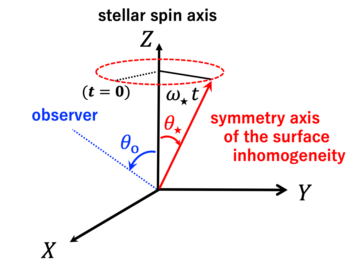
Figure 1: Schematic illustration of the star and the observer. The observer is located at $(\sin\theta_{\rm o},0,\cos\theta_{\rm o})$. In this frame, the stellar spin axis is chosen as the $Z$-axis, and the unit vector of symmetry axis is defined to be $(\sin\theta_{\star},0,\cos\theta_{\star})$ at $t=0$.

For an isotropically emitting stellar surface, the weighting kernel $K$ is equivalent to the visibility computed from the direction cosine between the unit normal vector of the stellar surface ($\bm{e}_{\star}$) and the unit vector toward the observer (${\bm{e}}_{\rm o}$). Without loss of generality, one can define a spherical coordinate system in which the symmetry axis is instantaneously set to be $z$-axis. In this case, one obtains

$$\bm{e}_{\star}\cdot\bm{e}_{\rm o}\equiv\mu_{\star}=\sin\gamma(t)\sin\theta[\cos\varphi+\Gamma(t)],$$ (4)

where

$$\Gamma(t)\equiv\cot\gamma(t)\cot\theta.$$ (5)

The location $(\theta,\varphi)$ on the surface is visible to the observer if $\mu_{\star}>0$. Therefore, the weighting kernel is simply written as

$$K(\theta,\varphi)=\max(\mu_{\star},0)=\sin\gamma(t)\sin\theta~{}\max[\cos\varphi+\Gamma(t),0].$$ (6)

If we adopt a quadratic limb darkening law, $I_{\rm LD}$ in equation (2) is specified by the two parameters $u_{1}$ and $u_{2}$ as

$$I_{\rm LD}(\theta,\varphi)=1-u_{1}(1-\mu_{\star})-u_{2}(1-\mu_{\star})^{2}=(1-u_{1}-u_{2})+(u_{1}+2u_{2})\mu_{\star}-u_{2}\mu_{\star}^{2}.$$ (7)

For instance, $u_{1}=0.47$ and $u_{2}=0.23$ for the Sun at $550$nm, and $u_{1}=0.05$ and $u_{2}=0.51$ for a typical white dwarf with $T_{\rm eff}=10^{4}$K and log $g$=8.0 in the LSST g-band (Cox, 2000; Gianninas et al., 2013).

We focus on a case where the surface intensity distribution is axisymmetric, i.e., $I(\theta,\varphi)=I(\theta)$. Then, equation (2) reduces to

$$L(t)=L_{0}(t)+L_{1}(t)+L_{2}(t),$$ (8)

where

$$L_{0}(t)=(1-u_{1}-u_{2})\frac{\sin\gamma}{\pi\overline{I}}\iint\max[\cos\varphi+\Gamma(t),0]~{}\sin^{2}\theta\,I(\theta)\,d\theta d\varphi,$$ (9)

$$L_{1}(t)=(u_{1}+2u_{2})\frac{\sin^{2}\gamma}{\pi\overline{I}}\iint\max[\cos\varphi+\Gamma(t),0]~{}\sin^{3}\theta\,[\cos\varphi+\Gamma(t)]I(\theta)\,d\theta d\varphi,$$ (10)

and

$$L_{2}(t)=-u_{2}\frac{\sin^{3}\gamma}{\pi\overline{I}}\iint\max[(\cos\varphi+\Gamma(t))^{3},0]~{}\sin^{4}\theta\,I(\theta)\,d\theta d\varphi.$$ (11)

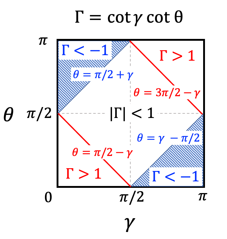
Figure 2: Range of $\theta$ and $\gamma$ for the visible part of the stellar sphere for the observer. The region with $\Gamma<-1$ corresponds to the position $(\theta,\varphi)$ that is invisible to the observer, while that with $\Gamma>1$ is always visible regardless of the value of $\varphi$. The region with $|\Gamma|<1$ becomes visible periodically when $\varphi<\varphi_{\rm c}$, where $\cos\varphi_{\rm c}\equiv-\Gamma$.

The visible part of the surface location $(\theta,\varphi)$ relative to the instantaneous observer’s line-of-sight is illustrated in Figure 2 (see also Figure 2 of Suto et al., 2022). By defining $\varphi_{\rm c}(t)$ for $|\Gamma(t)|\leq 1$ as

$$\cos\varphi_{\rm c}(t)\equiv-\Gamma(t)=-\cot\gamma(t)\cot\theta,$$ (12)

the instantaneously visible part of the surface is limited to $-\varphi_{\rm c}(t)<\varphi<\varphi_{\rm c}(t)$.

Consider first the case of $0<\gamma<\pi/2$. Then, equation (9) becomes

$$\frac{\pi\overline{I}}{1-u_{1}-u_{2}}L_{0}(t) = {\sin\gamma}\int_{0}^{\pi/2-\gamma}d\theta\int_{-\pi}^{\pi}d\varphi[\cos\varphi+\cot\gamma\cot\theta]\sin^{2}\theta\,{I(\theta)}$$ (15)

$$\qquad\qquad+{\sin\gamma}\int_{\pi/2-\gamma}^{\pi/2+\gamma}d\theta\int_{-\varphi_{\rm c}}^{\varphi_{\rm c}}d\varphi(\cos\varphi-\cos\varphi_{\rm c})\sin^{2}\theta\,{I(\theta)}$$

$$=2\pi{\cos\gamma}\int_{0}^{\pi/2-\gamma}\sin\theta\cos\theta{I(\theta)}\,d\theta+2\sin\gamma\int_{\pi/2-\gamma}^{\pi/2+\gamma}(\sin\varphi_{\rm c}-\varphi_{\rm c}\cos\varphi_{\rm c})\sin^{2}\theta\,{I(\theta)}\,d\theta.$$

Using the following relations derived from equation (12):

$$\sin^{2}\theta=\frac{\cot^{2}\gamma}{\cos^{2}\varphi_{\rm c}+\cot^{2}\gamma},\qquad d\theta=-\frac{\sin\varphi_{\rm c}\cot\gamma}{\cos^{2}\varphi_{\rm c}+\cot^{2}\gamma}d\varphi_{\rm c},$$ (16)

the second term in equation (15) becomes an integral in terms of $\varphi_{\rm c}$ alone:

$$\int_{\pi/2-\gamma}^{\pi/2+\gamma}\sin^{2}\theta(\sin\varphi_{\rm c}-\varphi_{\rm c}\cos\varphi_{\rm c})\,d\theta=\int_{\pi}^{0}\cot^{3}\gamma\frac{\sin\varphi_{\rm c}(\varphi_{\rm c}\cos\varphi_{\rm c}-\sin\varphi_{\rm c})}{(\cos^{2}\varphi_{\rm c}+\cot^{2}\gamma)^{2}}\,d\varphi_{\rm c}.$$ (17)

Finally, equation (15) reduces to

$$\frac{\overline{I}}{1-u_{1}-u_{2}}L_{0}(t) =2{\cos\gamma}\int_{0}^{\pi/2-\gamma}\sin\theta\cos\theta{I(\theta)}\,d\theta$$ (19)

$$\hskip 28.45274pt-\frac{2\sin\gamma\cot^{3}\gamma}{\pi}\int_{0}^{\pi}F_{0}(x;\gamma)I(\theta(x))dx,$$

where

$$F_{0}(x;\gamma)\equiv\frac{\sin x(x\cos x-\sin x)}{(\cos^{2}x+\cot^{2}\gamma)^{2}},\qquad\cos[\theta(x)]\equiv\frac{\cos x}{\cos^{2}x+\cot^{2}\gamma}.$$ (20)

Similarly, equation (10) is rewritten as

$$\frac{\overline{I}}{u_{1}+2u_{2}}L_{1}(t) = \frac{\sin^{2}\gamma}{\pi}\int_{0}^{\pi/2-\gamma}d\theta\int_{-\pi}^{\pi}d\varphi[\cos\varphi+\cot\gamma\cot\theta]^{2}\sin^{3}\theta\,{I(\theta)}$$ (22)

$$\qquad\qquad+\frac{\sin^{2}\gamma}{\pi}\int_{\pi/2-\gamma}^{\pi/2+\gamma}d\theta\int_{-\varphi_{\rm c}}^{\varphi_{\rm c}}d\varphi(\cos\varphi-\cos\varphi_{\rm c})^{2}\sin^{3}\theta\,{I(\theta)}$$

$$= \sin^{2}\gamma\int_{0}^{\pi/2-\gamma}\sin^{3}\theta{I(\theta)}\,d\theta+2{\cos^{2}\gamma}\int_{0}^{\pi/2-\gamma}\sin\theta\cos^{2}\theta{I(\theta)}\,d\theta$$ (24)

$$\qquad+\frac{\sin^{2}\gamma}{2\pi}\int_{\pi/2-\gamma}^{\pi/2+\gamma}(2\varphi_{\rm c}\cos 2\varphi_{\rm c}-3\sin 2\varphi_{\rm c})\sin^{3}\theta\,{I(\theta)}\,d\theta$$

$$= \sin^{2}\gamma\int_{0}^{\pi/2-\gamma}\sin^{3}\theta{I(\theta)}\,d\theta+2{\cos^{2}\gamma}\int_{0}^{\pi/2-\gamma}\sin\theta\cos^{2}\theta{I(\theta)}\,d\theta$$ (26)

$$\qquad-\frac{\sin^{2}\gamma\cot^{4}\gamma}{2\pi}\int_{0}^{\pi}F_{1}(x;\gamma)I(\theta(x))dx,$$

where

$$F_{1}(x;\gamma)\equiv\frac{\sin x(2x\cos 2x-3\sin 2x+4x)}{(\cos^{2}x+\cot^{2}\gamma)^{5/2}}.$$ (27)

Also equation (11) becomes

$$-\frac{\overline{I}}{u_{2}}L_{2}(t) = \frac{\sin^{3}\gamma}{\pi}\int_{0}^{\pi/2-\gamma}d\theta\int_{-\pi}^{\pi}d\varphi[\cos\varphi+\cot\gamma\cot\theta]^{3}\sin^{4}\theta\,{I(\theta)}$$ (29)

$$\qquad+\frac{\sin^{3}\gamma}{\pi}\int_{\pi/2-\gamma}^{\pi/2+\gamma}d\theta\int_{-\varphi_{\rm c}}^{\varphi_{\rm c}}d\varphi(\cos\varphi-\cos\varphi_{\rm c})^{3}\sin^{4}\theta\,{I(\theta)}$$

$$= 3\sin^{2}\gamma\cos\gamma\int_{0}^{\pi/2-\gamma}\sin^{3}\theta\cos\theta{I(\theta)}\,d\theta+2{\cos^{3}\gamma}\int_{0}^{\pi/2-\gamma}\sin\theta\cos^{3}\theta{I(\theta)}\,d\theta$$ (31)

$$+\frac{\sin^{3}\gamma}{12\pi}\int_{\pi/2-\gamma}^{\pi/2+\gamma}[27\sin\varphi_{\rm c}+11\sin 3\varphi_{\rm c}-6\varphi_{\rm c}(9\cos\varphi_{\rm c}+\cos 3\varphi_{\rm c})]\sin^{4}\theta\,{I(\theta)}\,d\theta$$

$$= 3\sin^{2}\gamma\cos\gamma\int_{0}^{\pi/2-\gamma}\sin^{3}\theta\cos\theta{I(\theta)}\,d\theta+2{\cos^{3}\gamma}\int_{0}^{\pi/2-\gamma}\sin\theta\cos^{3}\theta{I(\theta)}\,d\theta$$ (33)

$$\hskip 99.58464pt+\frac{\sin^{3}\gamma\cot^{5}\gamma}{12\pi}\int_{0}^{\pi}F_{2}(x;\gamma)I(\theta(x))dx,$$

where

$$F_{2}(x;\gamma)\equiv\frac{\sin x[6x(9\cos x+\cos 3x)-27\sin x-11\sin 3x]}{(\cos^{2}x+\cot^{2}\gamma)^{3}}.$$ (34)

In the same manner, we rewrite equations (9) to (11) for $\pi/2<\gamma<\pi$ as follows.

$$\frac{\overline{I}}{1-u_{1}-u_{2}}L_{0}(t) =2{\cos\gamma}\int_{3\pi/2-\gamma}^{\pi}\sin\theta\cos\theta{I(\theta)}\,d\theta$$ (36)

$$\hskip 28.45274pt-\frac{2\sin\gamma|\cot^{3}\gamma|}{\pi}\int_{0}^{\pi}F_{0}(x;\gamma)I(\theta(x))dx,$$

$$\frac{\overline{I}}{u_{1}+2u_{2}}L_{1}(t) = \sin^{2}\gamma\int_{3\pi/2-\gamma}^{\pi}\sin^{3}\theta{I(\theta)}\,d\theta+2{\cos^{2}\gamma}\int_{3\pi/2-\gamma}^{\pi}\sin\theta\cos^{2}\theta{I(\theta)}\,d\theta$$ (38)

$$\hskip 28.45274pt-\frac{\sin^{2}\gamma\cot^{4}\gamma}{2\pi}\int_{0}^{\pi}F_{1}(x;\gamma)I(\theta(x))dx,$$

$$-\frac{\overline{I}}{u_{2}}L_{2}(t) = 3\sin^{2}\gamma\cos\gamma\int_{3\pi/2-\gamma}^{\pi}\sin^{3}\theta\cos\theta{I(\theta)}\,d\theta+2{\cos^{3}\gamma}\int_{3\pi/2-\gamma}^{\pi}\sin\theta\cos^{3}\theta{I(\theta)}\,d\theta$$ (40)

$$\hskip 42.67912pt+\frac{\sin^{3}\gamma\cot^{5}\gamma}{12\pi}\int_{0}^{\pi}F_{2}(x;\gamma)I(\theta(x))dx,$$

3 Application to simple models of the surface inhomogeneity

3.1 Cap-model: a constant-intensity circular spot

Let us consider a simple model (Figure 3) in which the surface intensity is given as

$$I(\theta)=\left\{\begin{array}[]{ll}I_{s}&(0<\theta<\Delta\theta_{\rm s})\\ I_{0}&(\Delta\theta_{\rm s}<\theta<\pi)\end{array}\right..$$ (43)

This corresponds to a large spot of constant intensity $I_{s}$ around the north pole on the otherwise homogeneous surface of intensity $I_{0}$. Without loss of generality, we assume that the size of the spot is less than half of the entire surface ($\Delta\theta_{\rm s}<\pi/2$); the result for $\Delta\theta_{\rm s}>\pi/2$ is obtained simply by exchanging $I_{s}$ and $I_{0}$ and replacing $\Delta\theta_{\rm s}$ with $\pi-\Delta\theta_{\rm s}$ in the following expressions.

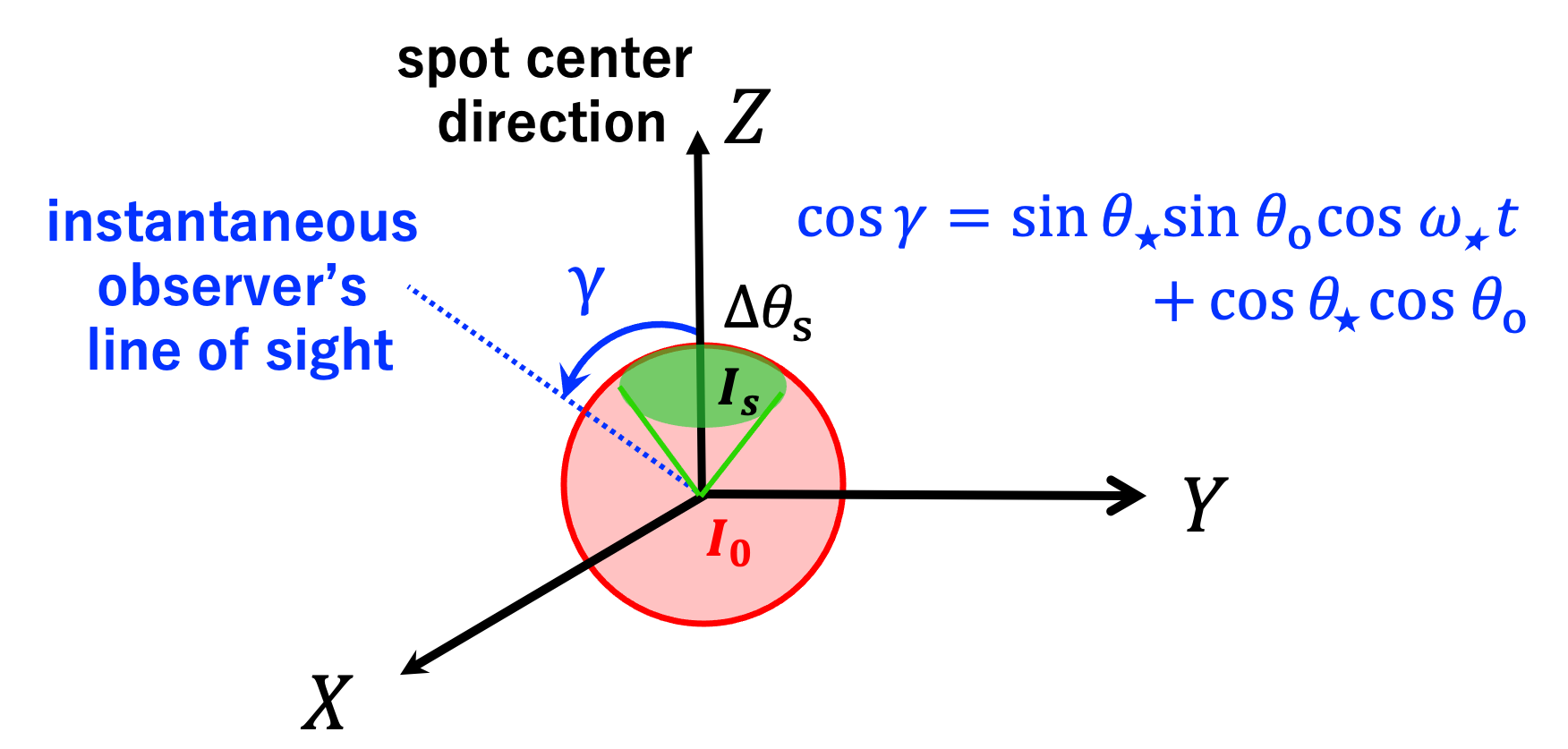
Figure 3: An instantaneous view of the spot configuration for the cap-model. The spot is located at the pole region ($\theta<\Delta\theta_{\rm s}$) with the constant intensity $I_{\rm s}$, while the intensity of the other surface is $I_{0}$.

We compute equation (19) without limb darkening (the derivation is given in appendix A), and summarize the final expressions below.

(a)

$0<\gamma<\pi/2$ and $\Delta\theta_{\rm s}<\pi/2-\gamma$:

$$L_{\rm 0a}(t)=\frac{I_{0}}{\overline{I}}-\frac{I_{0}-I_{s}}{\overline{I}}\sin^{2}\Delta\theta_{\rm s}\cos\gamma.$$ (44)

(b)

$0<\gamma<\pi/2$ and $\pi/2-\gamma<\Delta\theta_{\rm s}<\pi/2$:

$$L_{\rm 0b}(t)=\frac{I_{0}}{\overline{I}}-2\sin\gamma\cot^{3}\gamma\frac{(I_{0}-I_{s})}{\pi\overline{I}}\int_{\varphi_{\rm c,s}}^{\pi}F_{0}(x;\gamma)dx,$$ (45)

where $\cos\varphi_{\rm c,s}\equiv-\cot\gamma\cot\Delta\theta_{\rm s}$.

(c)

$\pi/2<\gamma<\pi$ and $\Delta\theta_{\rm s}<\gamma-\pi/2$:

$$L_{\rm 0c}(t)=\frac{I_{0}}{\overline{I}}.$$ (46)

(d)

$\pi/2<\gamma<\pi$ and $\gamma-\pi/2<\Delta\theta_{\rm s}<\pi/2$:

$$L_{\rm 0d}(t)=\frac{I_{0}}{\overline{I}}-2\sin\gamma\cot^{3}\gamma\frac{(I_{0}-I_{s})}{\pi\overline{I}}\int_{0}^{\varphi_{\rm c,s}}F_{0}(x;\gamma)dx.$$ (47)

The case (a) corresponds to the situation that the whole spot is visible to the observer, and thus the modulation is proportional to the projected area of the spot ($\propto\cos\gamma$). This clearly indicates that the resulting modulation is proportional to $\cos\omega_{\star}t$; see equation (1). In contrast, the spot is completely invisible and there is no observed modulation in the case (c). In the other two cases (b) and (d), the part of the spot is periodically visible, and the corresponding lightcurves become a sinusoidal form truncated at upper/lower amplitudes.

We note that the cap-model can be generalized to a star with multiple large spots in a straightforward manner by summing up the photometric variations due to the $i$-th spot with $I_{{\rm s},i}$, $\theta_{{\rm s},i}(t)$, $\Delta\theta_{{\rm s},i}$, and the initial phase of $\varphi_{i}$.

3.2 p-model: an inhomogeneous surface with a globally varying intensity

Another simple model that we consider here assumes the parameterized surface intensity $I(\theta)$:

$$I(\theta)=I_{0}-\Delta I\cos^{p}\theta,$$ (48)

where $I_{0}$ is the intensity at the equator ($\theta=\pi/2$), and $\Delta I$ is the amplitude of the intensity variation on the surface.

If $p$ is an odd integer, $I(\theta)$ varies monotonically from $I_{0}-\Delta I$ (at $\theta=0$) to $I_{0}+\Delta I$ (at $\theta=\pi$), which is roughly consistent with previous data (e.g., Landolfi et al., 1993; Valyavin et al., 2008, 2011, 2014). In this case, equation (19) is rewritten as

$$L_{\rm 0p}(t) =\frac{I_{0}}{\overline{I}}-\frac{\Delta I}{\overline{I}}\frac{2(1-\sin^{p+2}\gamma)\cos\gamma}{p+2}$$ (50)

$$\qquad\qquad-\frac{\Delta I}{\overline{I}}\frac{2\sin\gamma\cot^{3}\gamma}{\pi}\int_{0}^{\pi}F_{0}(x;\gamma)\left(\frac{\cos x}{\sqrt{\cos^{2}x+\cot^{2}\gamma}}\right)^{p}dx,$$

where the second line is obtained from equation (76). Interestingly, after integrating by parts, we find the analytical result:

$$\int_{0}^{\pi}F_{0}(x;\gamma)\left(\frac{\cos x}{\sqrt{\cos^{2}x+\cot^{2}\gamma}}\right)^{p}dx=\frac{\pi}{p+2}\frac{\sin^{p+2}\gamma}{\cot^{2}\gamma},$$ (51)

if $p$ is an odd integer. Thus, equation (50) reduces to the following simple expression:

$$L_{\rm 0p}(t)=\frac{I_{0}}{\overline{I}}-\frac{\Delta I}{\overline{I}}\frac{2}{p+2}\cos\gamma.$$ (52)

As in the cap-model, it has a modulation component proportional to $\cos\gamma$, and thus to $\cos\omega_{\star}t$, but the parameter $p$ cannot be measured because it is completely degenerate with the modulation amplitude $\Delta I$, as long as it is an odd integer.

3.3 Lightcurve variations without limb darkening

In our modeling, the time-dependence of the lightcurve $L(t)$ is completely specified by that of $\gamma(t)$. Thus we define the scaled lightcurve variation in terms of $\gamma$:

$$\Delta\tilde{L}(\gamma)\equiv\frac{L(\gamma)-L(\gamma=0)}{L(\gamma=\pi)-L(\gamma=0)},$$ (53)

which is plotted in Figure 4 for our cap-model and p-model without limb darkening. For the p-model, $\Delta\tilde{L}(\gamma)$ simply reduces to $(1-\cos\gamma)/2$ regardless of the value of $p$, as shown in equation (52). In contrast, $\Delta\tilde{L}(\gamma)$ depends on the value of $\Delta\theta_{\rm s}$ as well; see equations (44) to (47).

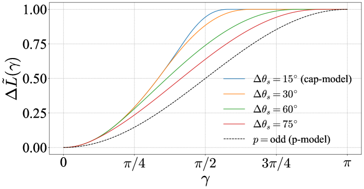
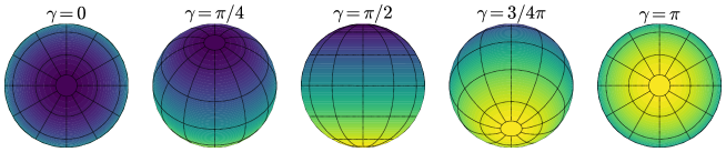
Figure 4: Scaled lightcurve variation $\Delta\tilde{L}(\gamma)$ against $\gamma$ for $I_{\rm s}<I_{0}$. The four solid lines correspond to the cap-model with $\Delta\theta_{\rm s}=15^{\circ}$, $30^{\circ}$, $60^{\circ}$, and $75^{\circ}$, while the dashed line corresponds to the p-model. The bottom panel shows a schematic illustration of the stellar surface at different phases for the p-model.

In reality, however, the value of $\gamma$ is not known to the observer, and $\Delta\tilde{L}(\gamma)$ is not directly observable. Instead, we define the scaled lightcurve variation in terms of $t$:

$$\tilde{L}(t)\equiv\frac{L(\omega_{\star}t)-L_{\rm 0a}(\omega_{\star}t=0)}{L_{\rm 0a}(\omega_{\star}t=\pi)-L_{\rm 0a}(\omega_{\star}t=0)},$$ (54)

which can be evaluated by fitting equation (44) to the sinusoidal portion of the measured data. Figure 5 plots $\tilde{L}(t)$ for the cap-model against $\omega_{\star}t$ without limb darkening.

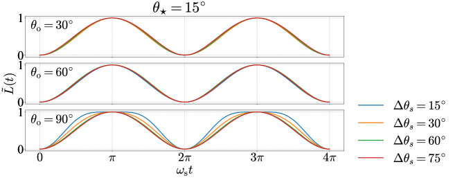
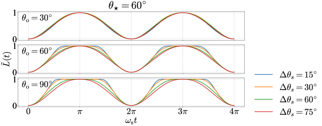
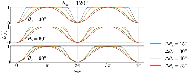
Figure 5: Scaled lightcurve variation $\tilde{L}(t)$ for the cap-model against the orbital phase ($\omega_{\star}t$) with $I_{\rm s}<I_{0}$. The top, middle, and bottom panels correspond to $\theta_{\star}=15^{\circ}$, $60^{\circ}$, and $120^{\circ}$ respectively, for $\theta_{\rm o}=30^{\circ}$, $60^{\circ}$, and $90^{\circ}$. Each panel has four curves corresponding to the spot size of $\Delta\theta_{\rm s}=15^{\circ}$, $30^{\circ}$, $60^{\circ}$, and $75^{\circ}$.

There is a certain degeneracy among parameters in the cap-model. If the lightcurve becomes saturated corresponding to equation (46), we can measure the threshold value of $\omega_{\star}t=\theta_{\rm crit}$ which gives

$$\sin\Delta\theta_{\rm s}=|\cos\gamma_{\rm crit}|\equiv|\sin\theta_{\star}\sin\theta_{\rm o}\cos\theta_{\rm crit}+\cos\theta_{\star}\cos\theta_{\rm o}|.$$ (55)

Then fitting to equation (44) with equation (55) provides a relation among $I_{s}/I_{0}$, $\theta_{\star}$ and $\theta_{\rm o}$:

$$L_{\rm 0a}(t) =\frac{I_{0}}{\overline{I}}-\frac{I_{0}-I_{s}}{\overline{I}}\sin^{2}\Delta\theta_{\rm s}\left(\sin\theta_{\star}\sin\theta_{\rm o}\cos\omega_{\star}t+\cos\theta_{\star}\cos\theta_{\rm o}\right)$$ (58)

$$=\left(\frac{I_{0}}{\overline{I}}-\frac{I_{0}-I_{s}}{\overline{I}}\sin^{2}\Delta\theta_{\rm s}\cos\theta_{\star}\cos\theta_{\rm o}\right)$$

$$\qquad\times\left[1-\frac{(1-I_{s}/I_{0})\sin^{2}\Delta\theta_{\rm s}\sin\theta_{\star}\sin\theta_{\rm o}}{1-(1-I_{s}/I_{0})\sin^{2}\Delta\theta_{\rm s}\cos\theta_{\star}\cos\theta_{\rm o}}\cos\omega_{\star}t\right].$$

The above equation explicitly indicates the degeneracy of the parameters involved in the amplitude of the sinusoidal curve. Therefore, the departure from the purely sinusoidal curve (see Figure 5) corresponding to equations (45) to (47) is important for the accurate determinations of the model parameters. We will discuss the parameter degeneracy in §3.5 below.

3.4 Limb darkening effect for the p-model

We compute the effect of limb darkening for the p-model. Substituting equation (48) to equations (22), (29), (38), and (40), we find

$$L_{\rm 1p}(\gamma) = (u_{1}+2u_{2})\left[\frac{2}{3}\frac{I_{0}}{\overline{I}}-\frac{\Delta I}{\overline{I}}J_{\rm 1p}(\gamma)\right],$$ (59)

$$L_{\rm 2p}(\gamma) = -u_{2}\left[\frac{1}{2}\frac{I_{0}}{\overline{I}}-\frac{\Delta I}{\overline{I}}J_{\rm 2p}(\gamma)\right],$$ (60)

where

$$J_{\rm 1p}(\gamma) =\frac{2+2p\cos^{2}\gamma-\sin^{p+3}\gamma[3(p+1)\cos^{2}\gamma+2]}{(p+1)(p+3)}\frac{\cos\gamma}{|\cos\gamma|}$$ (62)

$$\qquad\qquad\qquad-\frac{\sin^{2}\gamma\cot^{5}\gamma}{2\pi|\cot\gamma|}\int_{0}^{\pi}F_{1}(x;\gamma)\left(\frac{\cos x}{\sqrt{\cos^{2}x+\cot^{2}\gamma}}\right)^{p}dx$$

$$J_{\rm 2p}(\gamma) =\frac{6+2(p-1)\cos^{2}\gamma-\sin^{p+4}\gamma[5(p+2)\cos^{2}\gamma+6]}{(p+2)(p+4)}\cos\gamma$$ (65)

$$\qquad\qquad\qquad+\frac{\sin^{3}\gamma\cot^{5}\gamma}{12\pi}\int_{0}^{\pi}F_{2}(x;\gamma)\left(\frac{\cos x}{\sqrt{\cos^{2}x+\cot^{2}\gamma}}\right)^{p}dx$$

$$=\frac{6+2(p-1)\cos^{2}\gamma}{(p+2)(p+4)}\cos\gamma.$$

Thus, the normalized lightcurve for the p-model including quadratic limb darkening is given by

$$L_{\rm p}(\gamma) =\frac{I_{0}}{\overline{I}}\left[(1-u_{1}-u_{2})+\frac{2(u_{1}+2u_{2})}{3}-\frac{u_{2}}{2}\right]$$ (67)

$$\qquad-\frac{\Delta I}{\overline{I}}\left[\frac{2(1-u_{1}-u_{2})}{p+2}\cos\gamma+(u_{1}+2u_{2})J_{\rm 1p}(\gamma)-u_{2}J_{\rm 2p}(\gamma)\right],$$

where $p$ is an odd integer.

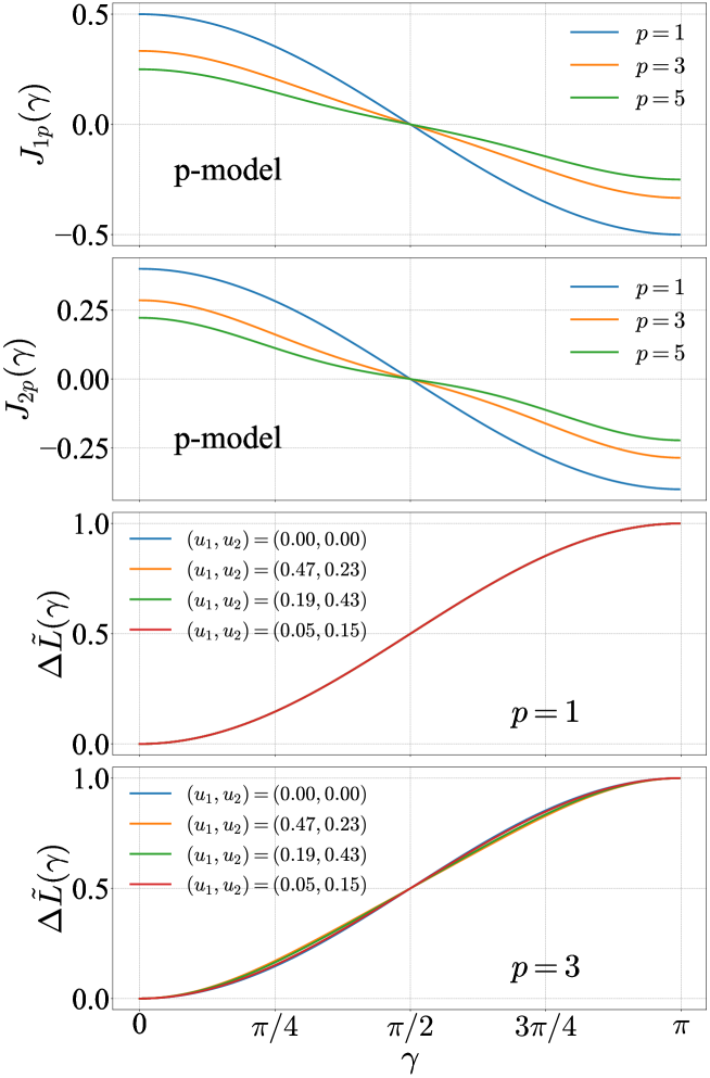
Figure 6: Effect of limb darkening for the p-model. The upper two panels are $J_{\rm 1p}$ and $J_{\rm 2p}$ against $\gamma$ with different values of $p$. The lower two panels plot the corresponding scaled lightcurve variations $\Delta\tilde{L}_{\rm p}$ for $p=1$ and 3, adopting the different sets of the limb darkening coefficients $(u_{1},\;u_{2})$.

The upper two panels in Figure 6 show $J_{\rm 1p}$ and $J_{\rm 2p}$ against $\gamma$ for the p-model with $p=1$ (blue), 3 (orange) and 5 (green). The corresponding scaled lightcurve variations $\Delta\tilde{L}_{\rm p}(\gamma)$, computed from equations (53) and (67) are plotted in the lower two panels for $p=1$ and 3, adopting the limb darkening coefficients of $(u_{1},\;u_{2})=(0.47,\;0.23)$ for the Sun, and $(0.19,\;0.43)$ and $(0.05,\;0.15)$ for WDs with $(T_{\rm eff},\;\log g)=(8\times 10^{3}{\rm K},\;9.2)$, and $(4.6\times 10^{4}{\rm K},\;9.5)$, respectively (Kilic et al., 2021; Caiazzo et al., 2021). For reference, $\Delta\tilde{L}_{\rm p}(\gamma)$ without limb darkening is plotted as well, while it is barely distinguishable from the other curves.

In the case of $p=1$, the scaled lightcurves seem to be identical to $(1-\cos\gamma)/2$, independently of the limb-darkening coefficients. This implies that both $J_{\rm 1p}$ and $J_{\rm 2p}$ are proportional to $\cos\gamma$ for $p=1$. Equation (65) indeed shows that it is the case for $J_{\rm 2p}$(p=1). We believe that it is also the case for $J_{\rm 1p}(p=1)$, while we are not yet able to prove it analytically. The scaled lightcurves with $p=3$, on the other hand, show very weak dependence on the limb-darkening coefficients, but they are still very well approximated by $(1-\cos\gamma)/2$. Therefore, we conclude that the limb-darkening effect is practically negligible in the p-model, and expect that it is the case for the cap-model as well.

3.5 Fitting the cap-model to the phase-folded lightcurves of a fast-spinning white dwarf ZTF J190132.9+145808.7

As an application of our current modeling, we attempt to fit the lightcurve of a fast-spinning white dwarf ZTF J190132.9+145808.7. We download the reduced photometric lightcurves that are made publicly available by Caiazzo et al. (2021). The total duration of the data is $\sim 80$ minutes, and the cadence is $\sim 1$ second. We use the data in the blue band alone, and omit the last 200 data points because they seem to be significantly contaminated by outliers. The long-term trend is then removed using the Savitzky-Golay filter (Savitzky & Golay, 1964), implemented as LightCurve.flatten in lightkurve modules (Lightkurve Collaboration et al., 2018). We adopt a window width of $1500$ seconds, and the data are folded according to the rotational period of $416.097$ seconds. Finally, we average the data over the bin width of $1$ second.

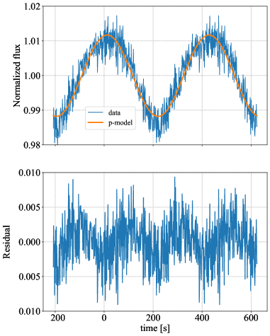
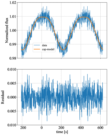
Figure 7: Best-fits to the phase-folded normalized lightcurve of ZTF J190132.9+145808.7, and their residuals for p-model (left) and cap-model (right).

As shown in the above subsection, the limb darkening effect is practically negligible. Thus, we ignore it in the present analysis. Figure 7 shows the best-fits and the residuals for the p-model (left) and the cap-model (right) from the nonlinear least square regression. While a purely sinusoidal curve predicted from the p-model does not fit the data, the cap-model is consistent with the feature of the observed lightcurve. Thus, we proceed to perform a Markov Chain Monte Carlo (MCMC) ensemble sampler for the cap-model using EMCEE (Foreman-Mackey et al., 2013).

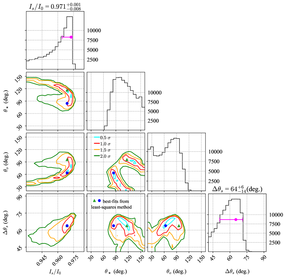
Figure 8: Posterior distribution among the four parameters, $I_{s}/I_{o}$, $\Delta\theta_{\rm s}$, $\theta_{\rm o}$ and $\theta_{\star}$, from the MCMC analysis in the cap-model. The observed lightcurve is averaged over a bin size of 5 seconds. The filled circle and triangle indicate solutions obtained from the nonlinear least square fit. Different curve correspond to the contours of $0.5\sigma$ (cyan) , $1.0\sigma$ (red), $1.5\sigma$ (orange), and $2.0\sigma$ (green) levels for two-dimensional histograms, respectively. The magenta symbols with error-bars indicate our best-fit parameters. The figure is generated using the CORNER package (Foreman-Mackey, 2016).

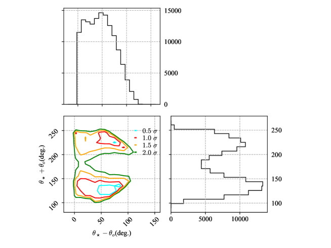
Figure 9: Same of Figure 8, but the posterior distribution of $\theta_{\star}-\theta_{\rm o}$ and $\theta_{\star}+\theta_{\rm o}$ in the cap-model.

The likelihood function is taken to be proportional to $\mathrm{exp}(-\chi^{2})$:

$$\chi^{2}=\sum_{i}\frac{(L_{\mathrm{cap},i}-L_{\mathrm{obs},i})^{2}}{\sigma_{i}^{2}},$$ (68)

where $L_{\mathrm{cap},i}$ is the cap-model prediction, $L_{\mathrm{obs},i}$ is the observed data, and $\sigma_{i}^{2}$ is the variance of the data in the $i$-th bin. The predicted lightcurve of the cap-model is normalized to fit the amplitude of the observed light curve. We adopt uniform priors for the four free parameters over the ranges of $0.8<I_{s}/I_{o}<1.2$, $0^{\circ}<\Delta\theta_{\rm s}<90^{\circ}$, and $0^{\circ}<\theta_{\rm o},~{}\theta_{\star}<180^{\circ}$.

The posterior distributions for $I_{s}/I_{o}$, $\Delta\theta_{\rm s}$, $\theta_{\rm o}$ and $\theta_{\star}$ from the MCMC analysis are shown in Figure 8, together with their marginalized probability density functions. The degree of the parameter degeneracy is clearly visible in Figure 8. The amplitude of the photometric variation and the departure from the sinusoidal curve are specified by $I_{s}/I_{o}$ and $\Delta\theta_{\rm s}$, respectively. Thus, these two parameters are well constrained from the fit. We define the best-fit parameters of $I_{s}/I_{o}$ and $\Delta\theta_{\rm s}$ by the mode and the corresponding $1\sigma$ errors from the histograms in Figure 8.

In contrast, the remaining two parameters, $\theta_{\star}$ and $\theta_{\rm o}$, are intrinsically degenerate, which can be understood from the fact that $\gamma$ is invariant by exchanging $\theta_{\rm o}$ and $\theta_{\star}$. Therefore, we put a constraint of $\theta_{\star}>\theta_{\rm o}$ in Figure 8. Even under the constraint, there are two peaks, roughly corresponding to $(\theta_{\rm o},\theta_{\star})$ $\approx(60^{\circ},90^{\circ})$ and $(90^{\circ},120^{\circ})$. In reality, however, these two are the same solution because $\theta_{\star}=60^{\circ}$ and $120^{\circ}$ lead to the identical lightcurve if $\theta_{\rm o}=90^{\circ}$ as shown in Figure 5. Thus, the peak at $(\theta_{\rm o},\theta_{\star})$ $\approx(90^{\circ},120^{\circ})$ is the same at $(90^{\circ},60^{\circ})$, which is simply equivalent to the other peak at $(\theta_{\rm o},\theta_{\star})$ $\approx(60^{\circ},90^{\circ})$.

This parameter degeneracy is shown more clearly in Figure 9, where we plot the posterior distribution on the $\theta_{\star}-\theta_{\rm o}$ vs $\theta_{\star}+\theta_{\rm o}$ plane. Therefore, the best-fits values of $\theta_{\rm o}$ and $\theta_{\star}$ are not easy to specify, and we decide to adopt their modes and the associated $1\sigma$ errors from the two-dimensional contours on the $\theta_{\rm o}$ – $\theta_{\star}$ plane in Figure 8. Having such degeneracy in mind, we summarize the best-fit parameters of the cap-model for ZTF J190132.9+145808.7 as follows:

$$I_{s}/I_{0} =0.971^{+0.001}_{-0.008},\qquad\Delta\theta_{\rm s}=64^{+6}_{-14}~{}\mathrm{deg.},$$ (69)

$$(\theta_{\rm o},\theta_{\star}) =(55^{+11}_{-31}~{}\mathrm{deg.},85^{+31}_{-7}~{}\mathrm{deg.})~{}{\rm or}~{}(90^{+18}_{-12}~{}\mathrm{deg.},120^{+24}_{-14}~{}\mathrm{deg.}).$$ (70)

The above solutions are indeed quite interesting. If $\theta_{\rm o}\approx 60^{\circ}$, the spot is located along the equatorial plane of the spin axis ($\theta_{\star}=90^{\circ}$). Even if we are viewing the WD from the edge-on direction ($\theta_{\rm o}\approx 90^{\circ}$), the obliquity of the spot is $\theta_{\star}\approx 60^{\circ}$, implying that the spot region is significantly away from the polar regions of the spin axis of the rotating WD.

We conclude that ZTF J190132.9+145808.7 has a relatively large dark spot. As inferred from the phase-resolved spectrum (Caiazzo et al., 2021), the dark spot is likely to be explained in terms of the magnetic dichroism. The spot structure may be also consistent with an off-centered dipole field as in the case of EUVE J0317-855 (Ferrario et al., 1997); the off-centered dipole field is an empirical configuration of the magnetic field, and assumes that its center differs from the stellar center by some offset along the dipole direction, while the surface brightness is still axisymmetric with respect to the dipole axis. Ferrario et al. (1997) found that the off-centered dipole field explains the lightcurve and polarization of EUVE J0317-855. If ZTF J190132.9+145808.7 has a similar configuration, its obliquity angle between the rotation and magnetic axis should be very large ($\theta_{\star}\approx 60^{\circ}$ or $90^{\circ}$), implying that the spot region, probably challenging a formation mechanism of such spots.

4 Discussion and conclusion

We have presented a formulation of photometric variations of rotating stars with an inhomogeneous surface intensity. We have provided a set of general expressions for the photometric lightcurve due to the oblique stellar rotation under the assumption that the inhomogeneity pattern is symmetric around an axis misaligned to the stellar spin direction. We have applied the formulation to two simple inhomogeneity models that are supposed to approximate the surface of WDs, and showed that they are able to reproduce the monochromatic sinusoidal lightcurves observed for a majority of variable WDs. Therefore, we conclude that the monochromatic sinusoidal lightcurve is a fairly generic prediction for obliquely rotating stars.

Furthermore, one of our surface models (the cap-model: §3.1) can model the departure from a purely sinusoidal lightcurve that are observed for a fraction of WDs including ZTF J190132.9+145808.7 (Caiazzo et al., 2021). The degree of the parameter degeneracy has been discussed extensively in §3.5. Our precise model prediction for the lightcurve shape will be also useful to distinguish between the oblique rotation model and the pulsation signature together with their difference in the frequency power spectra.

We note that the present method is not limited to white dwarfs alone, and applicable to predict photometric variations of a wide class of obliquely rotating stars, once their surface inhomogeneity distribution is specified. Indeed, our current models provide a very useful parameterization that characterizes a physical model of the surface distribution. Thus it is complementary to the inversion method (e.g., Kawahara & Fujii, 2010, 2011; Fujii & Kawahara, 2012; Aizawa et al., 2020; Luger et al., 2021) to infer the surface inhomogeneity distribution that does not require a priori model but is challenging to reconstruct the surface model from the limited signal-to-noise ratio of the observational data.

Even in purely sinusoidal lightcurves, the parameter degeneracy may be broken by combining spectro-polarimetric data. Since the surface inhomogeneity is likely originated from the stellar magnetic field, the measurements of the longitudinal and surface components of the time-varying magnetic fields may reveal the orientation of the dipolar magnetic fields, i.e., $\theta_{\rm o}$ and $\theta_{\star}$ (Landolfi et al., 1993) in a complementary manner. Then we may break the parameter degeneracy from the joint fits to the spectro-polarimetric and photometric data. This methodology has been successfully applied to WD 1953-011 (Valyavin et al., 2008) for instance, and will become applicable more precisely using our quantitative modeling of the photometric lightcurve.

According to our result, an appreciable non-sinusoidal signature appears on a lightcurve when both the obliquity angle $\theta_{\star}$ and the stellar spin inclination angle relative to the observer $\theta_{\rm o}$ is larger than the spot size $\Delta\theta_{\rm s}$. In this case, the spot becomes invisible from the observer for a certain rotation phase, and the photometric lightcurve in the phase exhibits plateaus. The plateaus appear either at the tops or the bottoms of the lightcurve when the spot has a lower or a higher intensity than the average of the stellar disk, respectively. The former corresponds to a dark spot ($I_{s}<I_{0}$) as in the case of ZTF J190132.9+145808.7. The latter cases with a bright spot ($I_{s}>I_{0}$), or a facula, could also occur for a strongly-magnetized fast-spinning WD, or a WD pulsar with a force-free magnetosphere, as inferred for neutron-star pulsars e.g., PSR J0030+0451 (Bilous et al., 2019; Miller et al., 2019; Riley et al., 2019) and PSR J0740+6620 (Riley et al., 2021; Miller et al., 2021). The non-sinusoidal fraction of lightcurves of WDs in a certain temperature and mass range should be a useful statistical measure of their magnetospheric structure. We plan to perform systematic comparison of our lightcurve models against the photometric data obtained by Kepler, TESS, ZTF, and Tomo-e Gozen (Aizawa et al., 2022), which will be reported elsewhere in due course.

Appendix A Analytic derivation of integrals appearing in the expressions for photometric variations

Lightcurves for the cap-model without limb darkening are computed from equation (19), and rewritten as follows, depending on the four different parameter ranges of $\gamma$ and $\Delta\theta_{\rm s}$.

(a)

$0<\gamma<\pi/2$ and $\Delta\theta_{\rm s}<\pi/2-\gamma$:

$$L_{\rm 0a}(t) = \frac{\cos\gamma}{2\overline{I}}\left[I_{s}(1-\cos 2\Delta\theta_{\rm s})+I_{0}(\cos 2\Delta\theta_{\rm s}+\cos 2\gamma)\right]$$ (72)

$$\qquad\qquad+\frac{2I_{0}\sin\gamma\cot^{3}\gamma}{\pi\overline{I}}\int_{0}^{\pi}F_{0}(x;\gamma)dx$$

(b)

$0<\gamma<\pi/2$ and $\pi/2-\gamma<\Delta\theta_{\rm s}<\pi/2$:

$$L_{\rm 0b}(t) = \frac{I_{s}\cos^{3}\gamma}{\overline{I}}+\frac{2\sin\gamma\cot^{3}\gamma}{\pi\overline{I}}\left({I_{s}}\int_{\varphi_{\rm c,s}}^{\pi}F_{0}(x;\gamma)dx+{I_{0}}\int_{0}^{\varphi_{\rm c,s}}F_{0}(x;\gamma)dx\right),$$ (73)

where $\cos\varphi_{\rm c,s}\equiv-\cot\gamma\cot\Delta\theta_{\rm s}$.

(c)

$\pi/2<\gamma<\pi$ and $\Delta\theta_{\rm s}<\gamma-\pi/2$:

$$L_{\rm 0c}(t)=\frac{I_{0}\cos^{3}\gamma}{\overline{I}}+\frac{2I_{0}\sin\gamma\cot^{3}\gamma}{\pi\overline{I}}\int_{0}^{\pi}F_{0}(x;\gamma)dx.$$ (74)

(d)

$\pi/2<\gamma<\pi$ and $\gamma-\pi/2<\Delta\theta_{\rm s}<\pi/2$:

$$L_{\rm 0d}(t) = \frac{I_{0}\cos^{3}\gamma}{\overline{I}}+\frac{2\sin\gamma\cot^{3}\gamma}{\pi\overline{I}}\left({I_{s}}\int_{0}^{\varphi_{\rm c,s}}F_{0}(x;\gamma)dx+{I_{0}}\int_{\varphi_{\rm c,s}}^{\pi}F_{0}(x;\gamma)dx\right).$$ (75)

Since equation (74) corresponds to a case where the spot is invisible to the observer, it should reduce to $I_{0}/\overline{I}$. This implies that the following definite integral of $F_{0}(x;\gamma)$ is given as

$$\int_{0}^{\pi}F_{0}(x;\gamma)dx=\int_{0}^{\pi}\frac{\sin x(x\cos x-\sin x)}{(\cos^{2}x+\cot^{2}\gamma)^{2}}dx=-\frac{\pi}{2}\frac{\sin^{2}\gamma}{|\cos\gamma|^{3}}(1-|\cos\gamma|^{3}).$$ (76)

Indeed, one can explicitly prove equation (76) by decomposing it in three integrals as follows.

$$\int_{0}^{\pi/2}\frac{x\sin x\cos x}{(\cos^{2}x+\cot^{2}\gamma)^{2}}dx =\sin^{4}\gamma\int_{0}^{\pi/2}\frac{x\sin x\cos x}{(\cos^{2}\gamma\sin^{2}x+\cos^{2}x)^{2}}dx$$ (78)

$$=\frac{\pi}{4}\frac{\sin^{4}\gamma}{\cos^{2}\gamma(1+|\cos\gamma|)}.$$

$$\int_{\pi/2}^{\pi}\frac{x\sin x\cos x}{(\cos^{2}x+\cot^{2}\gamma)^{2}}dx =-\pi\int_{0}^{\pi/2}\frac{\sin x\cos x}{(\cos^{2}x+\cot^{2}\gamma)^{2}}dx+\int_{0}^{\pi/2}\frac{x\sin x\cos x}{(\cos^{2}x+\cot^{2}\gamma)^{2}}dx$$ (80)

$$=-\frac{\pi}{2}\frac{\sin^{4}\gamma}{\cos^{2}\gamma}+\frac{\pi}{4}\frac{\sin^{4}\gamma}{\cos^{2}\gamma(1+|\cos\gamma|)}.$$

$$-\int_{0}^{\pi}\frac{\sin^{2}x}{(\cos^{2}x+\cot^{2}\gamma)^{2}}dx =\int_{0}^{\pi}\frac{dx}{\cos^{2}x+\cot^{2}\gamma}-(1+\cot^{2}\gamma)\int_{0}^{\pi}\frac{dx}{(\cos^{2}x+\cot^{2}\gamma)^{2}}$$ (82)

$$=\pi\frac{\sin^{2}\gamma}{|\cos\gamma|}-\frac{\pi}{2}\sin^{2}\gamma\frac{1+\cos^{2}\gamma}{|\cos\gamma|^{3}}.$$

Summing up the above three equations leads to equation (76). Finally, substituting equation (76) into equations (72) to (75) yields equations (44) to (47) shown in §3.1.

One can repeat the above argument that derives equation (76) for integrals of $F_{1}(x;\gamma)$ and $F_{2}(x;\gamma)$. When we set $I(\theta)=I_{0}$, equations (22) and (29) should be independent of $\gamma$. So we evaluate their right-hand-sides for $\gamma=0$, and find they reduce to $2I_{0}/3$ and $I_{0}/2$, respectively. Since the result should hold for an arbitrary value of $\gamma$, we obtain the following results:

$$\int_{0}^{\pi}F_{1}(x;\gamma)dx=\frac{2\pi}{3}\frac{\sin^{5}\gamma}{\cos^{4}\gamma}(5-3\sin^{2}\gamma),$$ (83)

$$\int_{0}^{\pi}F_{2}(x;\gamma)dx=\pi\frac{\sin^{2}\gamma}{|\cos^{5}\gamma|}(21|\cos^{5}\gamma|-15|\cos^{7}\gamma|-6).$$ (84)

These results are used in deriving equations (59) and (60).

We also find that a long but straightforward algebra reveals

$$\int_{0}^{\pi}F_{2}(x;\gamma)\left(\frac{\cos x}{\sqrt{\cos^{2}x+\cot^{2}\gamma}}\right)^{p}dx=\frac{12\pi\sin^{p+6}\gamma\cos^{4}\gamma}{(p+2)(p+4)}[6+5(p+2)\cos^{2}\gamma],$$ (85)

if $p$ is an odd integer. Thus, we obtain an analytic expression as the last line in equation (65). We were not able to find an analytic expression for equation (62), which is evaluated numerically in plotting Figure 6.

References

- Achilleos et al. (1992) Achilleos, N., Wickramasinghe, D. T., Liebert, J., Saffer, R. A., & Grauer, A. D. 1992, ApJ, 396, 273
- Aizawa et al. (2020) Aizawa, M., Kawahara, H., & Fan, S. 2020, ApJ, 896, 22
- Aizawa et al. (2022) Aizawa, M., Kawana, K., Kashiyama, K., Ohsawa, R., Kawahara, H., Naokawa, F., Tajiri, T., Arima, N., Jiang, H., Hartwig, T., Fujisawa, K., Shigeyama, T., Arimatsu, K., Doi, M., Kasuga, T., Kobayashi, N., Kondo, S., Mori, Y., Okumura, S.-i., Takita, S., & Sako, S. 2022, PASJ
- Barstow et al. (1995) Barstow, M. A., Jordan, S., O’Donoghue, D., Burleigh, M. R., Napiwotzki, R., & Harrop-Allin, M. K. 1995, MNRAS, 277, 971
- Bilous et al. (2019) Bilous, A. V., Watts, A. L., Harding, A. K., Riley, T. E., Arzoumanian, Z., Bogdanov, S., Gendreau, K. C., Ray, P. S., Guillot, S., Ho, W. C. G., & Chakrabarty, D. 2019, ApJ, 887, L23
- Brinkworth et al. (2013) Brinkworth, C. S., Burleigh, M. R., Lawrie, K., Marsh, T. R., & Knigge, C. 2013, ApJ, 773, 47
- Brinkworth et al. (2005) Brinkworth, C. S., Marsh, T. R., Morales-Rueda, L., Maxted, P. F. L., Burleigh, M. R., & Good, S. A. 2005, MNRAS, 357, 333
- Budding (1977) Budding, E. 1977, Ap&SS, 48, 207
- Caiazzo et al. (2021) Caiazzo, I., Burdge, K. B., Fuller, J., Heyl, J., Kulkarni, S. R., Prince, T. A., Richer, H. B., Schwab, J., Andreoni, I., Bellm, E. C., Drake, A., Duev, D. A., Graham, M. J., Helou, G., Mahabal, A. A., Masci, F. J., Smith, R., & Soumagnac, M. T. 2021, Nature, 595, 39
- Cox (2000) Cox, A. N. 2000, Allen’s astrophysical quantities, 4th edn. (Springer–Verlag)
- Donati et al. (1994) Donati, J. F., Achilleos, N., Matthews, J. M., & Wesemael, F. 1994, A&A, 285, 285
- Dorren (1987) Dorren, J. D. 1987, ApJ, 320, 756
- Eker (1994) Eker, Z. 1994, ApJ, 420, 373
- Euchner et al. (2002) Euchner, F., Jordan, S., Beuermann, K., Gänsicke, B. T., & Hessman, F. V. 2002, A&A, 390, 633
- Farr et al. (2018) Farr, B., Farr, W. M., Cowan, N. B., Haggard, H. M., & Robinson, T. 2018, AJ, 156, 146
- Ferrario et al. (1997) Ferrario, L., Vennes, S., Wickramasinghe, D. T., Bailey, J. A., & Christian, D. J. 1997, MNRAS, 292, 205
- Foreman-Mackey (2016) Foreman-Mackey, D. 2016, The Journal of Open Source Software, 1, 24
- Foreman-Mackey et al. (2013) Foreman-Mackey, D., Hogg, D. W., Lang, D., & Goodman, J. 2013, PASP, 125, 306
- Fujii & Kawahara (2012) Fujii, Y. & Kawahara, H. 2012, ApJ, 755, 101
- Fujii et al. (2011) Fujii, Y., Kawahara, H., Suto, Y., Fukuda, S., Nakajima, T., Livengood, T. A., & Turner, E. L. 2011, ApJ, 738, 184
- Fujii et al. (2010) Fujii, Y., Kawahara, H., Suto, Y., Taruya, A., Fukuda, S., Nakajima, T., & Turner, E. L. 2010, ApJ, 715, 866
- Gianninas et al. (2013) Gianninas, A., Strickland, B. D., Kilic, M., & Bergeron, P. 2013, ApJ, 766, 3
- Haggard & Cowan (2018) Haggard, H. M. & Cowan, N. B. 2018, MNRAS, 478, 371
- Hermes et al. (2021) Hermes, J. J., Putterman, O., Hollands, M. A., Wilson, D. J., Swan, A., Raddi, R., Shen, K. J., & Gänsicke, B. T. 2021, ApJ, 914, L3
- Hollands et al. (2020) Hollands, M. A., Tremblay, P. E., Gänsicke, B. T., Camisassa, M. E., Koester, D., Aungwerojwit, A., Chote, P., Córsico, A. H., Dhillon, V. S., Gentile-Fusillo, N. P., Hoskin, M. J., Izquierdo, P., Marsh, T. R., & Steeghs, D. 2020, Nature Astronomy, 4, 663
- Ivezić et al. (2019) Ivezić, Ž., Kahn, S. M., Tyson, J. A., Abel, B., Acosta, E., Allsman, R., Alonso, D., AlSayyad, Y., Anderson, S. F., Andrew, J., Angel, J. R. P., Angeli, G. Z., Ansari, R., Antilogus, P., Araujo, C., Armstrong, R., Arndt, K. T., Astier, P., Aubourg, É., Auza, N., Axelrod, T. S., Bard, D. J., Barr, J. D., Barrau, A., Bartlett, J. G., Bauer, A. E., Bauman, B. J., Baumont, S., Bechtol, E., Bechtol, K., Becker, A. C., Becla, J., Beldica, C., Bellavia, S., Bianco, F. B., Biswas, R., Blanc, G., Blazek, J., Blandford, R. D., Bloom, J. S., Bogart, J., Bond, T. W., Booth, M. T., Borgland, A. W., Borne, K., Bosch, J. F., Boutigny, D., Brackett, C. A., Bradshaw, A., Brandt, W. N., Brown, M. E., Bullock, J. S., Burchat, P., Burke, D. L., Cagnoli, G., Calabrese, D., Callahan, S., Callen, A. L., Carlin, J. L., Carlson, E. L., Chandrasekharan, S., Charles-Emerson, G., Chesley, S., Cheu, E. C., Chiang, H.-F., Chiang, J., Chirino, C., Chow, D., Ciardi, D. R., Claver, C. F., Cohen-Tanugi, J., Cockrum, J. J., Coles, R., Connolly, A. J., Cook, K. H., Cooray, A., Covey, K. R., Cribbs, C., Cui, W., Cutri, R., Daly, P. N., Daniel, S. F., Daruich, F., Daubard, G., Daues, G., Dawson, W., Delgado, F., Dellapenna, A., de Peyster, R., de Val-Borro, M., Digel, S. W., Doherty, P., Dubois, R., Dubois-Felsmann, G. P., Durech, J., Economou, F., Eifler, T., Eracleous, M., Emmons, B. L., Fausti Neto, A., Ferguson, H., Figueroa, E., Fisher-Levine, M., Focke, W., Foss, M. D., Frank, J., Freemon, M. D., Gangler, E., Gawiser, E., Geary, J. C., Gee, P., Geha, M., Gessner, C. J. B., Gibson, R. R., Gilmore, D. K., Glanzman, T., Glick, W., Goldina, T., Goldstein, D. A., Goodenow, I., Graham, M. L., Gressler, W. J., Gris, P., Guy, L. P., Guyonnet, A., Haller, G., Harris, R., Hascall, P. A., Haupt, J., Hernandez, F., Herrmann, S., Hileman, E., Hoblitt, J., Hodgson, J. A., Hogan, C., Howard, J. D., Huang, D., Huffer, M. E., Ingraham, P., Innes, W. R., Jacoby, S. H., Jain, B., Jammes, F., Jee, M. J., Jenness, T., Jernigan, G., Jevremović, D., Johns, K., Johnson, A. S., Johnson, M. W. G., Jones, R. L., Juramy-Gilles, C., Jurić, M., Kalirai, J. S., Kallivayalil, N. J., Kalmbach, B., Kantor, J. P., Karst, P., Kasliwal, M. M., Kelly, H., Kessler, R., Kinnison, V., Kirkby, D., Knox, L., Kotov, I. V., Krabbendam, V. L., Krughoff, K. S., Kubánek, P., Kuczewski, J., Kulkarni, S., Ku, J., Kurita, N. R., Lage, C. S., Lambert, R., Lange, T., Langton, J. B., Le Guillou, L., Levine, D., Liang, M., Lim, K.-T., Lintott, C. J., Long, K. E., Lopez, M., Lotz, P. J., Lupton, R. H., Lust, N. B., MacArthur, L. A., Mahabal, A., Mandelbaum, R., Markiewicz, T. W., Marsh, D. S., Marshall, P. J., Marshall, S., May, M., McKercher, R., McQueen, M., Meyers, J., Migliore, M., Miller, M., Mills, D. J., Miraval, C., Moeyens, J., Moolekamp, F. E., Monet, D. G., Moniez, M., Monkewitz, S., Montgomery, C., Morrison, C. B., Mueller, F., Muller, G. P., Muñoz Arancibia, F., Neill, D. R., Newbry, S. P., Nief, J.-Y., Nomerotski, A., Nordby, M., O’Connor, P., Oliver, J., Olivier, S. S., Olsen, K., O’Mullane, W., Ortiz, S., Osier, S., Owen, R. E., Pain, R., Palecek, P. E., Parejko, J. K., Parsons, J. B., Pease, N. M., Peterson, J. M., Peterson, J. R., Petravick, D. L., Libby Petrick, M. E., Petry, C. E., Pierfederici, F., Pietrowicz, S., Pike, R., Pinto, P. A., Plante, R., Plate, S., Plutchak, J. P., Price, P. A., Prouza, M., Radeka, V., Rajagopal, J., Rasmussen, A. P., Regnault, N., Reil, K. A., Reiss, D. J., Reuter, M. A., Ridgway, S. T., Riot, V. J., Ritz, S., Robinson, S., Roby, W., Roodman, A., Rosing, W., Roucelle, C., Rumore, M. R., Russo, S., Saha, A., Sassolas, B., Schalk, T. L., Schellart, P., Schindler, R. H., Schmidt, S., Schneider, D. P., Schneider, M. D., Schoening, W., Schumacher, G., Schwamb, M. E., Sebag, J., Selvy, B., Sembroski, G. H., Seppala, L. G., Serio, A., Serrano, E., Shaw, R. A., Shipsey, I., Sick, J., Silvestri, N., Slater, C. T., Smith, J. A., Smith, R. C., Sobhani, S., Soldahl, C., Storrie-Lombardi, L., Stover, E., Strauss, M. A., Street, R. A., Stubbs, C. W., Sullivan, I. S., Sweeney, D., Swinbank, J. D., Szalay, A., Takacs, P., Tether, S. A., Thaler, J. J., Thayer, J. G., Thomas, S., Thornton, A. J., Thukral, V., Tice, J., Trilling, D. E., Turri, M., Van Berg, R., Vanden Berk, D., Vetter, K., Virieux, F., Vucina, T., Wahl, W., Walkowicz, L., Walsh, B., Walter, C. W., Wang, D. L., Wang, S.-Y., Warner, M., Wiecha, O., Willman, B., Winters, S. E., Wittman, D., Wolff, S. C., Wood-Vasey, W. M., Wu, X., Xin, B., Yoachim, P., & Zhan, H. 2019, ApJ, 873, 111
- Kawahara & Fujii (2010) Kawahara, H. & Fujii, Y. 2010, ApJ, 720, 1333
- Kawahara & Fujii (2011) —. 2011, ApJ, 739, L62
- Kilic et al. (2021) Kilic, M., Kosakowski, A., Moss, A. G., Bergeron, P., & Conly, A. A. 2021, ApJ, 923, L6
- Kipping (2012) Kipping, D. M. 2012, MNRAS, 427, 2487
- Landolfi et al. (1997) Landolfi, M., Bagnulo, S., Landi Degl’Innocenti, M., Landi Degl’Innocenti, E., & Leroy, J. L. 1997, A&A, 322, 197
- Landolfi et al. (1993) Landolfi, M., Landi Degl’Innocenti, E., Landi Degl’Innocenti, M., & Leroy, J. L. 1993, A&A, 272, 285
- Liebert et al. (1977) Liebert, J., Angel, J. R. P., Stockman, H. S., Spinrad, H., & Beaver, E. A. 1977, ApJ, 214, 457
- Lightkurve Collaboration et al. (2018) Lightkurve Collaboration, Cardoso, J. V. d. M., Hedges, C., Gully-Santiago, M., Saunders, N., Cody, A. M., Barclay, T., Hall, O., Sagear, S., Turtelboom, E., Zhang, J., Tzanidakis, A., Mighell, K., Coughlin, J., Bell, K., Berta-Thompson, Z., Williams, P., Dotson, J., & Barentsen, G. 2018, Lightkurve: Kepler and TESS time series analysis in Python, Astrophysics Source Code Library
- Lu et al. (2022) Lu, Y., Benomar, O., Kamiaka, S., & Suto, Y. 2022, arXiv e-prints, arXiv:2206.05411
- Luger et al. (2021) Luger, R., Foreman-Mackey, D., Hedges, C., & Hogg, D. W. 2021, AJ, 162, 123
- Maoz et al. (2015) Maoz, D., Mazeh, T., & McQuillan, A. 2015, MNRAS, 447, 1749
- Miller et al. (2019) Miller, M. C., Lamb, F. K., Dittmann, A. J., Bogdanov, S., Arzoumanian, Z., Gendreau, K. C., Guillot, S., Harding, A. K., Ho, W. C. G., Lattimer, J. M., Ludlam, R. M., Mahmoodifar, S., Morsink, S. M., Ray, P. S., Strohmayer, T. E., Wood, K. S., Enoto, T., Foster, R., Okajima, T., Prigozhin, G., & Soong, Y. 2019, ApJ, 887, L24
- Miller et al. (2021) Miller, M. C., Lamb, F. K., Dittmann, A. J., Bogdanov, S., Arzoumanian, Z., Gendreau, K. C., Guillot, S., Ho, W. C. G., Lattimer, J. M., Loewenstein, M., Morsink, S. M., Ray, P. S., Wolff, M. T., Baker, C. L., Cazeau, T., Manthripragada, S., Markwardt, C. B., Okajima, T., Pollard, S., Cognard, I., Cromartie, H. T., Fonseca, E., Guillemot, L., Kerr, M., Parthasarathy, A., Pennucci, T. T., Ransom, S., & Stairs, I. 2021, ApJ, 918, L28
- Nakagawa et al. (2020) Nakagawa, Y., Kodama, T., Ishiwatari, M., Kawahara, H., Suto, Y., Takahashi, Y. O., Hashimoto, G. L., Kuramoto, K., Nakajima, K., Takehiro, S.-i., & Hayashi, Y.-Y. 2020, ApJ, 898, 95
- Price-Whelan et al. (2018) Price-Whelan, A. M., Sipőcz, B., Günther, H., Lim, P., Crawford, S., Conseil, S., Shupe, D., Craig, M., Dencheva, N., Ginsburg, A., et al. 2018, The Astronomical Journal, 156, 123
- Reding et al. (2020) Reding, J. S., Hermes, J. J., Vanderbosch, Z., Dennihy, E., Kaiser, B. C., Mace, C. B., Dunlap, B. H., & Clemens, J. C. 2020, ApJ, 894, 19
- Riley et al. (2019) Riley, T. E., Watts, A. L., Bogdanov, S., Ray, P. S., Ludlam, R. M., Guillot, S., Arzoumanian, Z., Baker, C. L., Bilous, A. V., Chakrabarty, D., Gendreau, K. C., Harding, A. K., Ho, W. C. G., Lattimer, J. M., Morsink, S. M., & Strohmayer, T. E. 2019, ApJ, 887, L21
- Riley et al. (2021) Riley, T. E., Watts, A. L., Ray, P. S., Bogdanov, S., Guillot, S., Morsink, S. M., Bilous, A. V., Arzoumanian, Z., Choudhury, D., Deneva, J. S., Gendreau, K. C., Harding, A. K., Ho, W. C. G., Lattimer, J. M., Loewenstein, M., Ludlam, R. M., Markwardt, C. B., Okajima, T., Prescod-Weinstein, C., Remillard, R. A., Wolff, M. T., Fonseca, E., Cromartie, H. T., Kerr, M., Pennucci, T. T., Parthasarathy, A., Ransom, S., Stairs, I., Guillemot, L., & Cognard, I. 2021, ApJ, 918, L27
- Roettenbacher et al. (2013) Roettenbacher, R. M., Monnier, J. D., Harmon, R. O., Barclay, T., & Still, M. 2013, ApJ, 767, 60
- Savitzky & Golay (1964) Savitzky, A. & Golay, M. J. E. 1964, Analytical Chemistry, 36, 1627
- Suto et al. (2022) Suto, Y., Sasaki, S., Nakagawa, Y., & Benomar, O. 2022, PASJ, 74, 857
- Valyavin et al. (2011) Valyavin, G., Antonyuk, K., Plachinda, S., Clark, D. M., Wade, G. A., Fox Machado, L., Alvarez, M., Lopez, J. M., Hiriart, D., Han, I., Jeon, Y.-B., Bagnulo, S., Zharikov, S. V., Zurita, C., Mujica, R., Shulyak, D., & Burlakova, T. 2011, ApJ, 734, 17
- Valyavin et al. (2014) Valyavin, G., Shulyak, D., Wade, G. A., Antonyuk, K., Zharikov, S. V., Galazutdinov, G. A., Plachinda, S., Bagnulo, S., Fox Machado, L., Alvarez, M., Clark, D. M., Lopez, J. M., Hiriart, D., Han, I., Jeon, Y.-B., Zurita, C., Mujica, R., Burlakova, T., Szeifert, T., & Burenkov, A. 2014, Nature, 515, 88
- Valyavin et al. (2008) Valyavin, G., Wade, G. A., Bagnulo, S., Szeifert, T., Landstreet, J. D., Han, I., & Burenkov, A. 2008, ApJ, 683, 466
- Wade et al. (2003) Wade, G. A., Bagnulo, S., Szeifert, T., Brinkworth, C., Marsh, T., Landstreet, J. D., & Maxted, P. 2003, in Astronomical Society of the Pacific Conference Series, Vol. 307, Solar Polarization, ed. J. Trujillo-Bueno & J. Sanchez Almeida, 569
- Williams et al. (2022) Williams, K. A., Hermes, J. J., & Vanderbosch, Z. P. 2022, AJ, 164, 131
- Winget & Kepler (2008) Winget, D. E. & Kepler, S. O. 2008, ARA&A, 46, 157