Class-Specific Explainability for Deep Time Series Classifiers

Abstract

Explainability helps users trust deep learning solutions for time series classification. However, existing explainability methods for multi-class time series classifiers focus on one class at a time, ignoring relationships between the classes. Instead, when a classifier is choosing between many classes, an effective explanation must show what sets the chosen class apart from the rest. We now formalize this notion, studying the open problem of class-specific explainability for deep time series classifiers, a challenging and impactful problem setting. We design a novel explainability method, DEMUX, which learns saliency maps for explaining deep multi-class time series classifiers by adaptively ensuring that its explanation spotlights the regions in an input time series that a model uses specifically to its predicted class. DEMUX adopts a gradient-based approach composed of three interdependent modules that combine to generate consistent, class-specific saliency maps that remain faithful to the classifier’s behavior yet are easily understood by end users. Our experimental study demonstrates that DEMUX outperforms nine state-of-the-art alternatives on five popular datasets when explaining two types of deep time series classifiers. Further, through a case study, we demonstrate that DEMUX’s explanations indeed highlight what separates the predicted class from the others in the eyes of the classifier.

I Introduction

Background. Deep learning methods represent the state-of-the-art for tackling time series classification problems in important domains from finance [1] to healthcare [2, 3]. In these applications, we typically aim to classify a time series to be a member of one of many classes, referred to as multi-class classification in contrast to binary classification [4]. Despite the success of these deep learning methods, domain experts may not trust predictions from deep models as they are “opaque” and thus hard to understand. This lack of trust has the potential to hinder wide deployment of promising deep models for real-world applications [5]. By helping users better understand and thus trust their models, explainability has been recognized as a critical tool for successfully deploying deep learning models [6, 7, 8, 9, 10, 11, 12, 13].

To explain a time series classification, we highlight the time steps that the model associates with the class it predicts via a saliency map [14, 9, 7]. However, in the multi-class problem setting where a classifier is choosing between many classes, an effective explanation must show what sets the chosen class apart from the rest of the classes. Thus the explanation should only highlight that particular subset of time steps that explains why that class was predicted compared to other classes. To further illustrate this with an example from computer vision, consider classifying images as either cats, dogs, foxes, or wolves. Fur is certainly evidence that an animal is in the image, but given choices between only these animals, fur is specific to no class. Therefore, an explanation should avoid highlighting fur [15]. In computer vision, it has been recognized as critical to leverage relationships between classes [15]. We conjecture that the same is equally true for time series, yet existing methods for time series ignore all relationships between classes [6, 9, 8, 10, 12]. Further, by ignoring this class-specificity issue, users may be prone to rationalize a model’s prediction in the face of erroneous explanations, having been instilled with a false sense of confidence [16].

Figure 1: Effective explanations of multi-class time series classifiers should show what regions of a time series set that class apart from the rest. Here, we show a deep classifier that predicts Heart Attack given an ECG. Explanations for individual classes (middle column) may have overlapping regions. However, as shown on right, the middle of the signal is what sets Heart Attack apart according to the classifier.

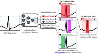
Motivating Example. Consider a deep multi-class time series classifier for ECG data [17] that classifies heartbeats into three classes: Heart Attack, Cardiac Arrest, and Normal Heart. Without knowing whether the classifier learned to recognize relevant critical regions of the time series for each class, a doctor may not trust its prediction. As shown in Figure 1 (middle), state-of-the-art methods would explain each class independently [8, 7, 13, 12]. However, by ignoring the relationships between classes, it appears as if the model uses most of the signal when predicting its top class, Heart Attack, even when it shares the same critical regions with Cardiac Arrest and Normal Heart classes as shown in blue. A class-specific explanation, on the other hand, should correct for the model using the same regions for multiple classes. In our example, it (rightmost column) explains that the burst (non-overlapping critical region) of the signal is what the model uses to predict Heart Attack instead of other classes.

State-of-the-Art. Explainablility for time series models has recently emerged as a promising direction to help users trust deep time series classifier models [8, 9, 7, 6, 10, 18, 12]. The most successful methods learn to perturb input time series to explain an opaque model’s behavior in the vicinity of one instance [7, 8]. Intuitively, time steps that have a higher impact on model accuracy will be ranked higher. Most existing methods [8, 9, 18, 12, 13, 5] explain model behavior by perturbing each time step using either static, predefined values like zero or other time series instances from a “background” dataset. For example, PERT [7], which explains only binary deep time series classifiers, perturbs each time step by replacing it from a replacement time series sampled from the background dataset. DYNAMASK [8, 19], which also treats each class independently, uses static replacement strategies for each time step for deriving explanations for a multivariate classifier. It makes a binary decision if a feature is important or not. To-date, class-specific explanations, despite their recognized need in fields like computer vision [15], remain an open problem in time series. Typically, a successful multi-class classifier assigns high probability to one of the classes and lower probabilities to the rest. Evidence derived to explain the predicted class should be unique to that class, relative to other classes. But existing time series explainable methods fail to incorporate the knowledge about relationships between classes.

Beyond lacking class-specificity, another well-known disadvantage of perturbation-learning methods is the high variance between explanations derived over multiple runs for the same time series instance as input [20, 19, 21]. High variability among explanations decreases a user’s trust in an explainability method and must therefore be reduced.

Problem Definition. We study the open problem of Class-Specific Explainability for Multi-Class Time Series Classifiers: given a time series and a pre-trained multi-class classifier, we aim to generate a class-specific saliency map for the classifier’s predicted class. A saliency map is a vector with one element per time step in the time series instance, where higher values of an element indicates a higher importance of this time step according to the classifier. To be class-specific, the saliency map should assign high importance only to time steps uniquely important to the predicted class (in contrast to also being important to other classes). This problem has multiple possibly conflicting objectives: a good saliency map should be class-specific, highlight only the most-relevant time steps, and still remain faithful to the model’s behavior.

Challenges. Our problem is challenging for several reasons:

• Class-Specificity: Generating class-specific saliency maps requires knowledge of explanations across all classes. However, learning concurrently multiple explanations is hard, in particular for low-probability classes, with a model’s predictions often highly variable in regions of low probability.

• Local Fidelity: We consider multi-class classifiers that predict probability distributions. Learning perturbations to explain these models must incorporate all class probabilities to remain faithful to the classifier’s behavior. However, minor changes to the input can have a large effect on the predicted class distribution.

• Temporal Coherence: Time steps often depend on their neighbors’ values. This implies that similarly for saliency maps neighboring time steps should have similar importance. While this encourages discovering important subsequences, thereby improving explainability, it conflicts with local fidelity and class-specificity. Hence, a trade-off must inherently be considered in any effective solution.

• Consistent Saliency: Perturbation-based explainability methods can create saliency maps that vary dramatically for the same instances when re-initialized. Yet to be useful in real-world applications, we should instead consistently generate similar explanations for the same time series

Proposed Solution. To derive class-specific explanations, we propose Distinct TEmporal MUlticlass EXplainer (DEMUX), a novel model-agnostic, perturbation-based explainability method for multi-class time series models. DEMUX jointly learns saliency maps, with a focus on removing shared salient regions to generate a class-specific explanation for the model’s top predicted class.

DEMUX is gradient-based approach that monitors changes in the classifier’s predictions while perturbing values at each time step. It produces a saliency map for the classifier’s top predicted class that preserves the classifier’s prediction probability distribution across classes. To generate good perturbations, DEMUX learns to sample a replacement time-series per class from a background dataset using a clustering-based replacement selector. DEMUX avoids out-of-distribution replacement values by ensuring perturbations are like other time series the model has seen before for each class and for each time step, leading to more stable saliency maps.

Contributions. Our main contributions are as follows:

• We identify and characterize the problem of class-specific saliency maps for deep multi-class time series classifiers.

• We introduce the first effective solution, DEMUX, which extends beyond recent work with three innovations: learning to remove shared saliency across classes (Class-Specificity), generating class-specific perturbations that are locally faithful (Local Fidelity and Temporal Coherence), and ensuring stability of saliency maps (Consistent Saliency) for given time series instances.

• Using five real datasets, we conclusively demonstrate that DEMUX outperforms nine state-of-the-art alternatives, successfully generating class-specific explanations for multiple types of deep time-series classifiers.

II Related Works

Deep learning models have achieved remarkable results in domains from time series forecasting to classification tasks. But these models are opaque in nature. Given that a substantial amount of data collected in high-stake domains like healthcare, [2, 3] finance [22] and autonomous vehicles [23, 24] are in the form of time series, the need to build explainable AI (XAI) for the time series domain is rapidly increasing. Saliency maps [19, 21] are among the many promising approaches to increasing transparency of a deep learning model. They correspond to importance scores that highlight the series regions contributing to the classifier’s predictions. Below we characterize XAI methods according to the strategy they utilize to generate importance scores representing model explanations.

Perturbation methods. These methods [8, 7, 19] slightly change the input time series and compare the output to the baseline to create an importance ranking. The resulting saliency masks indicate importance of the time steps, explaining prediction for the given test instance. In time series, each time step can have a range of valid or in-distribution values. Assuming static baselines replacement values or random time series from background datasets are good enough for each class-specific replacement tends to lead to sub-optimal importance scores for saliency maps.

Surrogate models. These methods [6, 12, 25] produce linear surrogate models that are trained to emulate the behavior of an opaque model locally for a set of perturbed versions of a given instance. If the linear model is a good enough local approximation, then its coefficients are treated as an explanation. Intuitively, if there is not a clear linear relationship between the set of perturbed instances and the opaque model’s predictions, which is often the case in complex time series deep learning models, a linear model’s coefficients fall short of generating a good explanation for a non-linear model’s predictions.

Other methods. There are some popular methods [9, 13, 18, 11] that do not fall in one of the above categories. SHAP [13] does random permutations of the input features and average the marginal contribution of features to build importance Shapley scores. TIMESHAP is built upon KernelSHAP and extends it to the time series domain.

Unfortunately, none of the above category of methods address class-specific explanations challenges i.e., there has been little work developing explainability methods specifically for multi-class setting in time series, despite the recognition of the class-specific explainability importance in computer vision domain [15, 19]. Without leveraging knowledge from other classes during multi-class explanation learning, explanations from existing methods are less effective [15]. To the best of our knowledge, our work is the first to study learnable class-specific perturbations to explain opaque multi-class time series classifiers. The methods mentioned above do not focus on generating class-specific perturbations and consistent explanations. Nor do they preserve the opaque model’s prediction probability distribution across the classes while generating explanations.

III Methodology

III-A Problem Definition

Assume we are given a set of $N$ time series $\mathcal{D}=\{\mathbf{x}_{1},\dots,\mathbf{x}_{N}\}$ and a deep multi-class time series classifier $f:\mathbb{X}\to\mathcal{Y}$, where $\mathbb{X}\in\mathbb{R}^{T}$ is the $T$-dimensional feature space with and $\mathcal{Y}=\{1,2,\dots,C\}$ is the label space with $C$ classes. Let us consider an instance-of-interest $\mathbf{x}\in\mathcal{D}$, a time series with $T$ time steps along with a predicted probability distribution $\mathbf{\hat{y}}=f(\mathbf{x})$ over $C$ classes where $\mathbf{\hat{y}}\in[0,1]^{C}$ and $\sum_{i=1}^{C}\mathbf{\hat{y}}_{i}=1$. The top predicted class $z$ where $z=\operatorname*{\arg\!\max}\mathbf{\hat{y}}$ has predicted confidence $\mathbf{\hat{y}_{z}}$ and is the class for which we seek an explanation.

Our goal is to learn a class-specific saliency map $\bm{\theta}\in[-1,1]^{T}$ for the class of interest $z$ where each element represents the importance of a corresponding time step. Positive values in $\bm{\theta}$ indicate evidence for class $z$, while negative values indicate evidence against class $z$. We follow the lead of recent work on perturbation-based explanations for time series [8, 7], and assume the importance of a time step $t$ should reflect the expected scale of the change of $P(\mathbf{\hat{y}}_{z}|\mathbf{x})$ when $\mathbf{x}$ is perturbed: $|P(\mathbf{\hat{y}}_{z}|\mathbf{x})-P(\mathbf{\hat{y}}_{z}|\mathbf{\tilde{x}})|$, where $\mathbf{\tilde{x}}$ is perturbed version of $\mathbf{x}$. A successfully learned saliency map $\bm{\theta}$ will assign high values to the regions in a time series where perturbations dramatically shift the model’s predictions away from $z$. To ensure that explanations are simple and intuitive, we favor contiguous subsequences within the saliency map, indicating that neighboring time steps likely have similar importance, and that $\bm{\theta}$ be sparse if possible, assigning no importance to unimportant time steps.

Figure 2: DEMUX Architecture. Three model components collaborate to produce a saliency map for the predicted class. 1) The Cluster-Based Replacement Selector picks replacement time series. 2) The Class-Specific Perturbation Function uses these replacements to perturb the input. 3) The Mask Memory Unit produces Consistent Saliency Map.

III-B Proposed Method: DEMUX

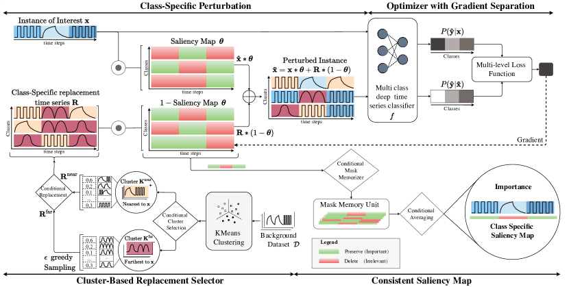
We propose the Distinct Temporal Multi-class Explainer (DEMUX), the first method to produce class-specific explanations for deep multi-class time series classifiers. DEMUX is model agnostic, so can explain any multi-class deep time series classifier $f$’s predictions for an instance $\mathbf{x}$. By learning to discourage overlapping salient time steps between classes, DEMUX produces saliency maps that highlight the important class-specific time steps. As illustrated in Figure 2, DEMUX uses a novel class-specific replacement strategy to perturb time series and explain $f$’s behavior. DEMUX’s learning strategy encourages $\bm{\theta}$ to abide by a range of attractive behaviors and is accomplished via the design of a novel loss function that leads to explanations that are unique to the predicted class, simple and easy to understand, while being consistent between multiple runs.

DEMUX contains three key components that work together: (1) the Cluster-Based Replacement Selector learns which time series from the background dataset $\mathcal{D}$ are the best for replacement-based perturbation. (2) The Class-Specific Perturbation Function learns a saliency map $\bm{\theta}$ for the top predicted class $z$ relative to other classes by perturbing $\mathbf{x}$ and discovering the impact of each time step on $f$’s prediction probability distribution $P(\mathbf{\hat{y}}|\mathbf{x})$ across all classes. (3) A Mask Memory Unit to derive consistent Saliency Maps which is achieved by building a repository of good saliency maps during learning that matches the predicted probability distribution $P(\mathbf{\hat{y}}|\mathbf{x})$ of $f$.

Cluster-Based Replacement Selector. Perturbation alters the values of the instance-of-interest $\mathbf{x}$, generating a synthetic time series $\mathbf{\tilde{x}}$. However, choosing which time steps to alter and the scale of the modifications can be highly impactful. In fact, dramatically changing $\mathbf{x}$ often creates an out-of-distribution perturbation, on which $f$’s predictions are untrustworthy. PERT [7] overcomes this challenge by creating in-distribution perturbations via replacement time series $\mathbf{r}$, which replace time steps in $\mathbf{x}$ with time steps from background instances in $\mathcal{D}$. Inspired by PERT, we select a pair of time series from the background dataset $\mathcal{D}$ to provide evidence both for and against the class of interest $z$. However, multi-class replacement time series sampling is non-trivial as there can be many classes to choose from.

The best replacement time series may also vary by time step and per class, so we select replacement series $\mathbf{r}$ on a per-class and time step-by-time step basis. To provide evidence both for and against the class of interest $z$, the Cluster-Based Replacement Selector employs a clustering on $\mathcal{D}$—we use KMeans with Kneedle [26] to find a suitable number of clusters $k$ for the given dataset $\mathcal{D}$ in our experiments. Thereafter, for each class, the Cluster-Based Replacement Selector chooses two clusters of time series representatives $\mathbf{K}^{\text{near}}$ and $\mathbf{K}^{\text{far}}$ from these $k$ clusters. $\mathbf{K}^{\text{near}}$ denotes a cluster nearest to $\mathbf{x}$ and $\mathbf{K}^{\text{far}}$ a cluster furthest from $\mathbf{x}$ based on the Euclidean distance between $\mathbf{x}$ and the centroid of the two clusters, respectively. Then, we pick one replacement time series from $\mathbf{K^{\text{near}}}$ and one from $\mathbf{K}^{\text{far}}$

$$\mathbf{r}^{\text{far}}:=\begin{cases}\mathbf{r}^{\text{far}}\ &\text{with probability }1-\epsilon\\ \text{random }\mathbf{r}\in\mathbf{K}^{\text{far}}&\text{with probability }\epsilon\end{cases}$$ (1)

where $\mathbf{r}^{\text{far}}$ is one time series sampled from $\mathbf{K^{\text{far}}}$ with probability $\epsilon$. We also sample $\mathbf{r}^{\text{near}}$ from the nearest cluster $\mathbf{K^{\text{near}}}$. We repeat this process for each of the $C$ classes, accumulating the replacement series into respective matrices $\mathbf{R}^{near},\mathbf{R}^{far}\in\mathbb{R}^{C\times T}$, denoting two replacement time series $\mathbf{r}^{near}$ and $\mathbf{r}^{far}$ per class. We employ epsilon greedy-based prioritized sampling [27] to explore and learn which replacement time series sampled from $\mathcal{D}$ are best for instance-of-interest $\mathbf{x}$

Class-Specific Perturbation. Next, we derive a class-specific saliency map $\bm{\theta}$ for $z$, the top predicted class, relative to other classes in $\mathbf{\hat{y}}$. We perturb the instance of interest $\mathbf{x}$ by performing time step and class-specific replacement using replacement time series matrices and a saliency map $\bm{\theta}$. Equation 2 shows a class-specific perturbation where $\mathbf{x}^{*}_{i}$ is the perturbed instance for the $i$-th class. ${\mathbf{x}^{*}_{i}}$ is passed to classifier $f$ to observe the effects of the perturbation on $f$’s predicted distribution $P(\mathbf{\hat{y}}|\mathbf{x})$.

We learn a perturbation function $\Phi:\mathbb{R}^{C\times T}\to\mathbb{R}^{C\times T}$ where the key component of $\Phi$ is a two-dimensional parameterized matrix $\bm{\theta}\in[-1,1]^{C\times T}$. An element $\theta_{i,t}$ of this parameterized matrix represents the importance value of time step $t$ for class $i$ relative to other classes. Values in $\bm{\theta}$ close to 1 indicate strong evidence for the respective class $i$. Values close to -1 indicate evidence against the class $i$. Values near 0 imply no importance.

To consider both evidence for and against each class, our perturbation function $\Phi$ adaptively learns to replace values at each time step with replacement time series matrices. We thus replace the time step with $\mathbf{R^{\text{near}}}$, the representative of time series from the cluster nearest to $\mathbf{x}$ for $\theta_{i,t}<0$. Similarly, when $\theta_{i,t}\geq 0$, $\mathbf{x}$ is replaced with the corresponding time step of $\mathbf{R^{\text{far}}}$, the representative of time series from the cluster farthest to $\mathbf{x}$. This way, DEMUX learns the degree of sensitivity of each time step per class. The function $\Phi$ generates perturbation $\mathbf{\tilde{x}}$ by performing time step-specific interpolation for each class:

Here, $\mathbbm{1}_{\bm{\theta}_{i}<0}$ is a matrix-wise indicator function that returns 1 for elements of $\bm{\theta}_{i}$ that are less than 0 and $\mathbbm{1}_{\bm{\theta}_{i}\geq 0}$ returns 1 for elements of $\bm{\theta}_{i}$ greater than or equal to 0. $\odot$ is the Hadamard product. For readability, we refer to this operation as $\Phi(\mathbf{x};\bm{\theta})$. Inspired by [19], We add a small amount of Gaussian noise $g$ to avoid overfitting $\bm{\theta}$ to extremely specific values. Using Equation 2, the final values of $\mathbf{\tilde{x}}$, the perturbed version of $\mathbf{x}$, are thus interpolations between the original time steps of $\mathbf{x}$ and the replacement series $\mathbf{R}^{\text{near}}_{i}$ or $\mathbf{R}^{\text{far}}_{i}$ where $i$ is the $i$-th class in $\mathbf{\hat{y}}$ according to the scale of the corresponding value in $\bm{\theta}_{i}$. The conditional interval specific operations on $\bm{\theta}$ are necessary to derive evidence both for and against class $z$.

Learning Class-Specific Explanation. Class-specific saliency values $\bm{\theta}\in\mathbb{R}^{C{\times}T}$ are learned using a novel loss function (Equation 8) containing five key components. We optimize the loss function to derive a simple instance-specific explanation for the predicted distribution $P(\mathbf{\hat{y}}|\mathbf{x})$ for $\mathbf{x}$.

First, we encourage Class-Specificity: Overlapping salient regions between classes should be minimized. We design an objective called shared saliency deletion $L_{\text{SSD}}$, which learns to remove shared saliency amongst the top predicted class $z$ and the rest of the classes, proportional to the respective class probability. This uniquely differentiates the top class salient time steps from the other classes. DEMUX learns unique class-specific saliency map $\bm{\theta}_{z}$ for the top predicted class $z$ by altering $\bm{\theta}_{z}$ with respect to the corresponding importance values at the same time steps from other classes. Consider $\theta_{z,t}$ where $t$ is the time step, if the importance value for time step $t$ is high for multiple classes, it is considered to be a shared salient time step. The importance value $\theta_{z,t}$ is reduced by the importance value of time step $t$ from $\bm{\theta}_{i,t}$ where $i\neq z$ represents a different class, and is weighted by the respective class confidence $P(\mathbf{\hat{y}}_{i}|\mathbf{x})$ to counter the influence of least confidence classes. Intuitively, $L_{\text{SSD}}$ improves the importance of unique salient time steps and reduces the importance of shared salient time steps.

$$L_{SSD}=\lambda_{5}\left(\frac{1}{\left\|{\mathcal{Y}}\right\|}\left(\bm{\theta}_{z}-\left\|\sum_{\begin{subarray}{c}\\ i\neq z\end{subarray}}^{\mathcal{Y}}(\bm{\theta}_{z}-P(\mathbf{\hat{y}}_{i}|\mathbf{x})*\bm{\theta}_{i})\right\|\right)^{2}\right)$$ (3)

Second, to derive instance-specific explanations from $f$, it is crucial to preserve Local Fidelity by preserving $P(\mathbf{\hat{y}}|\mathbf{x})$ for $\mathbf{x}$. Any changes to the predicted probability distribution $P(\mathbf{\hat{y}}|\mathbf{x})$ creates a disconnect between the derived explanation $\bm{\theta}_{z}$ and instance-of-interest $\mathbf{x}$. The second component of our loss function, $L_{Prev}$, encourages the perturbation function $\Phi$ to produce perturbations for the top class $z$ while preserving the distribution $P(\mathbf{\hat{y}}|\mathbf{x})$ for $\mathbf{x}$. To achieve this preservation, we use the Kullback-Liebler (KL) Divergence (Equation 4) to measure how the predicted distribution for the perturbed instance $P(\mathbf{\hat{y}}|\mathbf{\tilde{x}})$ differs from the reference distribution $P(\mathbf{\hat{y}}|\mathbf{x})$.

$$L_{\text{Prev}}=\lambda_{1}\left(\left(f(\mathbf{x})-f(\Phi(\mathbf{x};\bm{\theta}_{z}))\right)_{KL}\right)$$ (4)

Third, to generate preserving low probabilities is a challenge as there are many possible perturbations that result in a low probabilities. Thus, for classes other than highest confidence class $z$ we encourage the saliency map $\bm{\theta}$ to highlight the time steps that are responsible for maximizing the specific-class probability represented by Equation 5. Intuitively, we preserve the confidence for the top predicted class $z$, to derive explanations specific to instance-of-interest $\mathbf{x}$. For the rest of the classes, we maximize the confidences to find the minimal salient time steps that causes the prediction probability for the respective class to increase significantly. By making use of gradient separation and multi-objective loss, we learn saliency maps for $z$ and the other classes distinctively.

$$L_{\text{Max}}=\lambda_{2}\left(\frac{1}{\left\|{\mathcal{Y}}\right\|}\sum_{i\neq z}^{\mathcal{Y}}\left(1-f(\Phi(\mathbf{x};\bm{\theta}_{i}))\right)\right)$$ (5)

Fourth, to encourage simple explanations, with minimal salient time steps per class, we incorporate the $L_{Budget}$ loss per class, similar to PERT [7] and DYNAMASK [8] methods. This component encourages the values of $\bm{\theta}$ to be as small as possible; intuitively, values that are not important should be close to 0 per our problem definition.

$$L_{\text{Budget}}=\lambda_{3}\left(\frac{1}{\left\|{\mathcal{Y}}\right\|}\sum_{i=0}^{\mathcal{Y}}\left(\frac{1}{\left\|T\right\|}\sum_{t=0}^{T}\left|\theta_{i,t}\right|\right)\right)$$ (6)

Fifth, we encourage the saliency map to be Temporally Coherent: neighboring time steps should generally have similar important. To achieve this coherence, we add a time series regularizer $L_{\text{TReg}}$ per class that minimizes the squared difference between neighboring saliency values:

$$L_{\text{TReg}}=\lambda_{4}\left(\frac{1}{\left\|{\mathcal{Y}}\right\|}\sum_{i=0}^{\mathcal{Y}}\left(\frac{1}{\left\|T\right\|}\sum_{t=0}^{T-1}(\theta_{i,t}-\theta_{i,t+1})^{2}\right)\right)$$ (7)

Finally, all the loss terms are summed, each being scaled by a $\lambda$ coefficient to balance the components depending on task-specific preferences in explanation behavior. Minimizing the total loss in Equation 8 leads to simple, class-specific saliency maps.

$$L(P(\mathbf{\hat{y}}|\mathbf{x});\bm{\theta})=L_{\text{SSD}}+L_{\text{Prev}}+L_{\text{Max}}+L_{\text{Budget}}+L_{\text{TReg}}$$ (8)

Mask Memory Unit for Consistent Saliency Maps. A common problem with perturbation-based methods [7, 8, 19] is high variance between explanations, even given the same inputs multiple times. Also, during learning between epochs, the saliency maps can change dramatically [20]. This makes training challenging, in particular, to know when to stop training. We address this problem using a Mask Memory Unit, in which we store “good” saliency maps throughout training. A saliency map is considered to be good if the resulting prediction $\operatorname*{\arg\!\max}f(\Phi(\mathbf{\tilde{x}}))$ for the perturbed instance $\mathbf{\tilde{x}}$ is identical to the predicted class $z$ for the instance of interest $\mathbf{x}$. The final saliency map generated corresponds to the average of the last few (10 or more) saliency maps in the repository. This significantly reduces the variance between the saliency maps offered by our model as it results in generating consistent explanations for same time series instance across multiple runs.

Dataset	ACSF1	Plane	Trace	ECG5000	Meat
Num. Train Instances	100	105	100	500	60
Num. Test Instances	100	105	100	4500	60
Num. Time steps	1460	144	275	140	500
Num. Classes	10	7	4	5	3

TABLE I: Dataset summary statistics.

Methods	Datasets
	ECG5000		Plane		Trace		ACSF1		Meat
	AUC $\uparrow$	IoU $\downarrow$	AUC $\uparrow$	IoU $\downarrow$	AUC $\uparrow$	IoU $\downarrow$	AUC $\uparrow$	IoU $\downarrow$	AUC $\uparrow$	IoU $\downarrow$
RISE [28]	0.60 (.005)	15.4%	0.25 (.009)	7.52%	0.49 (.004)	19.8%	0.16 (.007)	19.9%	0.17 (.010)	29.3%
LEFTIST [11]	0.84 (.003)	22.5%	0.39 (.011)	33.8%	0.31 (.007)	36.9%	0.17 (.014)	36.6%	0.36 (.006)	30.3%
LIME [12]	0.78 (.012)	29.9%	0.50 (.005)	30.8%	0.46 (.006)	37.1%	0.19 (.006)	37.9%	0.15 (.002)	38.4%
TSMULE [6]	0.43 (.017)	11.2%	0.27 (.009)	7.39%	0.38 (.015)	19.5%	0.05 (.008)	13.1%	0.12 (.003)	31.7%
SHAP [13]	0.45 (.133)	12.7%	0.38 (.011)	20.2%	0.52 (.045)	30.6%	0.04 (.005)	18.7%	0.25 (.002)	24.9%
TIMESHAP [9]	0.73 (.175)	20.5%	0.27 (.023)	9.6%	0.31 (.067)	17.6%	0.02 (.089)	17.2%	0.15 (.033)	19.2%
MP [19]	-0.38 (.021)	93.8%	0.16 (.001)	66.6%	0.34 (.009)	13.4%	0.06 (.011)	12.7%	0.23 (.044)	2.25%
DYNAMASK [8]	0.69 (.005)	7.41%	0.25 (.008)	3.23%	0.23 (.007)	4.54%	0.13 (.007)	1.62%	0.05 (.001)	0.27%
PERT [7]	0.69 (.010)	32.8%	0.13 (.007)	21.2%	0.18 (.001)	40.4%	0.16 (.047)	37.9%	0.33 (.021)	21.1%
DEMUX	0.78 (.007)	0.24%	0.71 (.001)	4.31%	0.52 (.004)	2.44%	0.45 (.012)	2.11%	0.58 (.007)	2.46%

TABLE II: Performance of the AUC-Difference $\uparrow$ and IoU $\downarrow$ metrics with the FCN model. Parentheses indicate $\sigma$.

Methods	Datasets
	ECG5000		Plane		Trace		ACSF1		Meat
	AUC $\uparrow$	IoU $\downarrow$	AUC $\uparrow$	IoU $\downarrow$	AUC $\uparrow$	IoU $\downarrow$	AUC $\uparrow$	IoU $\downarrow$	AUC $\uparrow$	IoU $\downarrow$
RISE [28]	-0.34 (.005)	3.71%	0.31 (.009)	19.8%	0.25 (.004)	1.73%	0.14 (.005)	20.5%	0.45 (.010)	1.42%
LEFTIST [11]	0.80 (.002)	29.9%	0.36 (.005)	28.8%	0.91 (.006)	2.16%	0.14 (.019)	27.3%	0.72 (.002)	1.28%
LIME [12]	0.67 (.028)	30.6%	0.25 (.005)	28.5%	0.86 (.007)	17.9%	0.08 (.004)	32.6%	0.66 (.001)	22.5%
TSMULE [6]	-0.42 (.040)	1.0%	0.29 (.008)	18.9%	0.32 (.029)	3.2%	0.08 (.003)	4.2%	0.52 (.002)	33.3%
SHAP [13]	-0.32 (.030)	2.15%	0.34 (.003)	17.7%	0.92 (.045)	15.4%	0.03 (.013)	25.7%	0.55 (.001)	3.15%
TIMESHAP [9]	-0.34 (.075)	34.77%	0.31 (.007)	16.8%	0.64 (.037)	24.5%	0.02 (.063)	5.1%	0.54 (.008)	3.6%
MP [19]	-0.31 (.005)	57.9%	0.22 (.001)	13.8%	0.14 (.009)	63.0%	0.10 (.020)	37.9%	0.57 (.021)	38.9%
DYNAMASK [8]	-0.35 (.001)	1.14%	0.02 (.011)	0.22%	0.77 (.007)	0.50%	0.13 (.023)	5.43%	-0.57 (.031)	0.30%
PERT [7]	0.73 (.001)	25.6%	0.18 (.007)	17.7%	0.52 (.070)	29.4%	-0.02 (.035)	38.0%	0.27 (.002)	26.4%
DEMUX	0.81 (.007)	0.01%	0.42 (.001)	9.16%	0.25 (.004)	4.52%	0.15 (.007)	2.43%	0.75 (.007)	1.81%

TABLE III: Performance of the AUC-Difference $\uparrow$ and IoU $\downarrow$ metrics with the RNN model. Parentheses indicate $\sigma$.

IV Experimental Study

IV-A Datasets

We evaluate our method DEMUX on five popular real-world multi-class time series datasets: ACSF1 [29], Plane [30], Trace [31], Rock [32], ECG5000 [33], Meat [34]. Each is a popular publicly-available dataset [30] for multi-class time series classification. The summary statistics are provided in Table I. We use the default train and test split provided. For each, we train a three-layered Fully Connected Network (FCN) and a Recurrent Neural Network (RNN) to serve as multi-class deep time series classifiers in need of explanations. Three-layered FCN is considered as a strong baseline in time series classification [35]. Both models are then trained to achieve state-of-the-art accuracy [30] on their respective datasets.

IV-B Compared Methods

We compare our proposed method, DEMUX, to nine state-of-the-art explanation methods.

• DYNAMASK [8]. This method is an extension of MP [19] but incorporates the time dependency at each time step for each feature and learns to perturb each time step with static values or adjacent time step values such that $P(\mathbf{\hat{y}}|\mathbf{x})$ decreases. Saliency values are then used as the final explanation.

• PERT [7]. This method is designed for binary univariate time series and learns to dynamically replace each time step using time step specific interpolation. It learns to perturb each time step such that $P(\mathbf{\hat{y}}|\mathbf{x})$ is preserved to derive instance-specific for and against evidence.

• TSMULE [6]. This method is an extension of LIME [12] to identify superpixel-like patterns, i.e., semantically related data regions, in time series data. Matrix profile, SAX transformation and uniform segmentation algorithms are used to generate time segments for the perturbation.

• TIMESHAP [9]. This method builds upon SHAP and extends it to time series to explain important time steps contributing to the prediction. A temporal coalition pruning method aggregates time events to produce sequences of important data regions.

• SHAP [13]. SHAP assigns Shapley values [36] to each time step, thus computing their contributions to $P(\mathbf{\hat{y}}|\mathbf{x})$. Each time step in the instance of interest is replaced by a representative value observed at the corresponding time step, sampled from the background dataset.

• RISE [28]. The partial derivative of the opaque model’s prediction $P(\mathbf{\hat{y}}|\mathbf{x})$ with respect to each time step is estimated empirically by randomly setting time steps to zero and summarizing its impact on the $P(\mathbf{\hat{y}}|\mathbf{x})$.

• LEFTIST [11]. The partial derivative of $P(\mathbf{\hat{y}}|\mathbf{x})$ with respect to segments of time steps is estimated empirically by randomly replacing the corresponding values from a random instance from the background dataset, or with constants and summarizing its impact on $P(\mathbf{\hat{y}}|\mathbf{x})$.

• LIME [12]. Saliency values are derived from the coefficients of a linear surrogate model, trained to mimic the opaque model’s behaviour in the feature space surrounding $\mathbf{x}$. The approach’s success relies on the opaque model behaving linearly locally, which is rarely guaranteed.

• Meaningful Perturbation (MP) [19]. MP learns to perturb each time step such that $P(\mathbf{\hat{y}}|\mathbf{x})$ decreases. Perturbation is achieved by combining squared exponential smoothing with additive Gaussian noise. Saliency values are then learned iteratively and are used as the final explanation.

IV-C Implementation Details

For each dataset, we train a three-layer FCN and a 10-node single-layer RNN with GRU cells to serve as fairly standard multi-class time series classifiers [35] in need of explanations. Each dataset comes with a pre-defined split ratio. We train each model only on the training data, then explain their predictions for all test instances for each compared explainability method. All reported metrics are the result of the average over five runs to estimate the variance of the explainability methods. We optimize our proposed method using Adam [37] with a learning rate of $1e^{-3}$ and train for 5000 epochs, which we find empirically achieves convergence. We use the Weights & Biases framework [38] for experiment tracking. Our proposed method is implemented in PyTorch. For each compared method, we have used grid search to compute the optimum values of hyperparameters to get the best possible results. Our source code is publicly-available at https://github.com/rameshdoddaiah/DEMUX. This repository includes runtime benchmarks to show the time cost of DEMUX compared to other methods and Hyperparameter tuning table.

(a) $L_{\text{Prev}}$ coefficient ($\lambda_{1}$).

(b) $L_{\text{Max}}$ coefficient ($\lambda_{2}$).

(c) $L_{\text{Budget}}$ coefficient ($\lambda_{3}$).

(d) $L_{\text{SSD}}$ coefficient ($\lambda_{5}$).

Figure 3: DEMUX hyperparameter study results on ACSF1 dataset.

Figure 4: DEMUX ablation study results on ACSF1 dataset.

Figure 5: Meat [34] “Chicken” Class Case Study. The time series is shown in blue and saliency values are plotted against time steps in red for the top predicted chicken class and in green for another class, Turkey. DEMUX (the last row) highlights three unique, discriminative subsequences as the class-specific explanation, outlines by blue dashed boxes for the top predicted “Chicken” class, unlike the other methods. DEMUX highlights evidence for all classes, but only “Turkey” class is shown here due to space constraints.

IV-D Metrics

We use two key popular metrics to evaluate saliency maps for time series under the intuition that a prediction is well-explained if it accurately ranks the class-specific time steps by their importance, as defined by changes in $P(\mathbf{\hat{y}}|\mathbf{x})$, and also returns only the most important time steps and the intersection of overlapping salient regions across the classes are minimal.

Measuring Insertion and Deletion Sensitivity Impact: AUC-Difference Metric [39, 28, 7]. Saliency maps can be evaluated by “inserting” or “deleting” time steps from the time series instance based on the derived importance map and observing the changes in the opaque model’s predictions [39, 28, 7]. A good saliency map is one that has ranked time steps such that when the most important time steps are inserted or deleted, there is a sharp change in the confidence of the model’s prediction. This can be measured by computing the area under the deletion curve (AUDC) as time steps are deleted one by one. A lower value for this area indicates a better explanation. Analogously, insertion of a few important time steps should result in the largest possible increase in the confidence of the model’s prediction, thereby creating a large area under the insertion curve (AUIC). To ease comparisons, we merge these two measures into one metric by computing the difference, Equation 9 represents the difference between AUIC and AUDC where we expect the difference, AUC-Difference should be large (1.0), implying the saliency maps having a high AUIC (1.0) and a low AUDC (0.0) is a good explanation as per PERT [7, 39] and RISE [28].

$$\text{AUC-Difference}=\text{AUIC}-\text{AUDC}$$ (9)

The metric alleviates the need for human evaluation and the error-prone collection of human ground-truth. This makes it fairer and truer to the classifier’s own view on the problem. A pivotal choice in insertion and deletion tests is which reference input to use when deleting or inserting values to avoid spurious model classification. To achieve deletion during evaluation, we replace a to-be-deleted time step with the farthest cluster’s centroid derived from the background data set $D$ to provide in-distribution replacement values. Conversely, for insertion, we start with the the farthest cluster’s centroid and iteratively replace the time steps with the values of the instance-of-interest.

Measuring Class-Specificity of an Explanation: Intersection over Union. We leverage a standard intersection over union (IoU) metric from the image domain [15]. A simple and a good class-specific saliency map is the one that has no overlapping salient time steps across the classes with respect to the predicted class. This can be measured by intersection over union [15] of salient time steps of the predicted class saliency map with other classes’ saliency maps. First, we map each per-class salient time steps to a boolean value, either 1 or 0 based on a preset range of thresholds [min=0, max=1, step=0.1]. Second, we find intersection of per-class saliency map with predicted class saliency map and count (IC) number of non-zero salient time steps. Third, we find the union of per-class saliency map with predicted class saliency map and count (UC) number of non-zero salient time steps.

Equation 10 represents the ratio of overlapping salient time steps. We repeat step two and three with different thresholds ranging from 0 to 1 at every 0.1 interval to compute area under the curve (IoU curve). Minimal overlapping salient time steps leads to a higher the number of class-specific salient time steps. The area under the curve IoU metric must be minimal to quantitatively say the generated explanation is unique.

$$\text{Intersection over Union ( IoU )}=\frac{IC}{UC}$$ (10)

IV-E Experimental Results

IV-E1 DEMUX finds locally faithful explanations per-class.

To address the challenge of generating explanations being locally faithful to the classifier’s behavior, we first measure how well all compared explainability methods have ranked the time steps by their importance via the AUC-Difference metric [28, 7]. Our results using Fully-Connected and Recurrent Neural Networks can be found in Tables II and III, respectively, where we evaluate each method on five multi-class datasets. In most of the cases, DEMUX significantly outperforms all other methods on AUC-Difference by learning better rankings for time step importance. In general, learning to perturb, as done in DEMUX and PERT, outperforms the random-replacement methods RISE [28, 11], LIME [12], and SHAP [9] for both the long and short time series. This robust performance demonstrates that learned perturbations effectively produce higher-quality explanations than unlearned perturbations.

IV-E2 DEMUX finds class-specific salient time steps.

We next find that most state-of-the-art methods generate per-class saliency maps independently, leading to overlapping salient regions across the classes. As shown in Tables II and III, we also compare all methods according to the IoU metric [15], which measures how much saliency maps overlap between classes. As expected, DEMUX largely outperforms existing methods by learning to remove overlaps during training. Interestingly, DYNAMASK is competitive in three out of the five datasets, though it has much lower AUC-Difference. Because DYNAMASK seems to sacrifice AUC for IoU, there appears to be a trade-off between these two metrics, as expected. By and large, DEMUX significantly outperforms the state-of-the-art methods on both metrics, especially when considering them together.

IV-E3 DEMUX learns consistent explanations.

Some recent works express concern that perturbation methods can lead to different explanations [20] for the same instances when respective saliency masks are initialized randomly. We share this worry and provide some peace of mind: DEMUX achieves more-consistent explanations across multiple runs than other methods. Each saliency mask is re-initialized five times on all time series in each dataset. We report the standard deviation for the AUC-Difference metric as shown in Tables II and III. DEMUX has a far-lower average standard deviation across all datasets when AUC-Difference and IoU are considered together.

IV-E4 Ablation study.

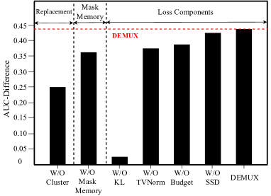
To demonstrate the need for each component of DEMUX, we perform an ablation study, removing different DEMUX components and reporting the AUC-Difference on the ACSF1 dataset [29]. We focus on the replacement strategy, mask memory unit, and each loss component. Our results in Figure 4 show that each component is necessary to achieve a good performance.

First, without the per-class time series replacement learning to sample component (W/O Cluster) AUC-Difference suffers when random time series with irrelevant time steps are used for replacement. This shows the need for selecting class-specific replacement values per time step to create per-class perturbations. Second, without the mask memory unit component (W/O Mask Memory), we pick the final saliency map at $5000^{th}$ epoch as explanation and the AUC-Difference metric decreases slightly. This shows that Perturbation-based method may not consistently pick a good saliency map if stopped after a predefined number of epochs. Third, we compare DEMUX’s performance while removing different components of the loss function. As expected, W/O KL clearly has a substantial impact on the final AUC-Difference, as without this component, there is no relationship between the saliency map and the model’s prediction probability distribution. Fourth, the W/O TVNorm and W/O Budget components have less of an impact but still contribute to DEMUX’s state-of-the-art performance by learning simple and discriminative subsequences. Fifth, learning without a class-specific loss component W/O SSD reduces DEMUX’s AUC-Difference further, stressing the need for learning class-specific saliency maps. DEMUX includes all the above components and indeed achieves the best AUC-Difference.

IV-E5 Hyperparameter Study.

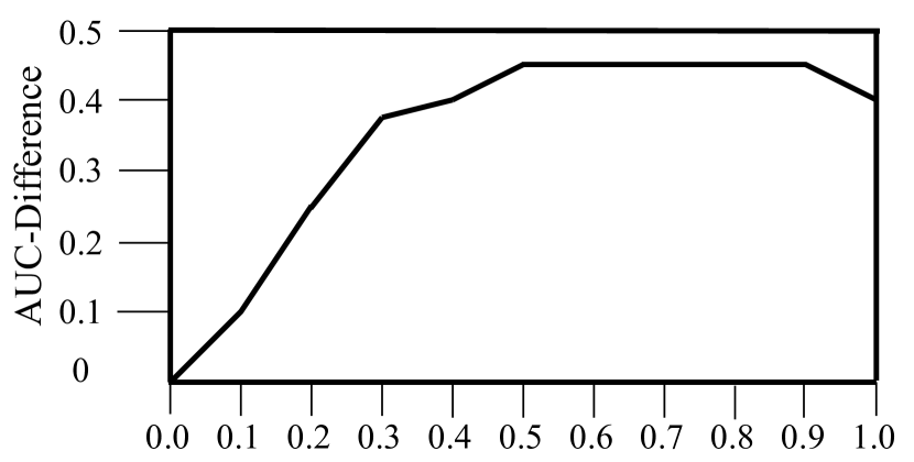
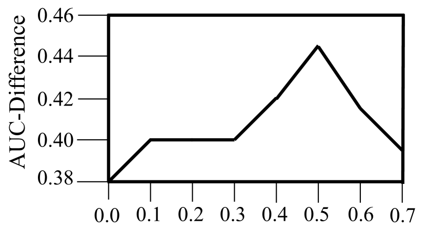
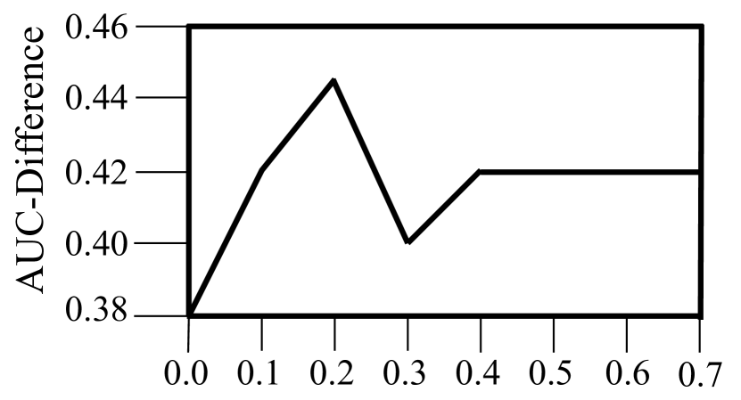
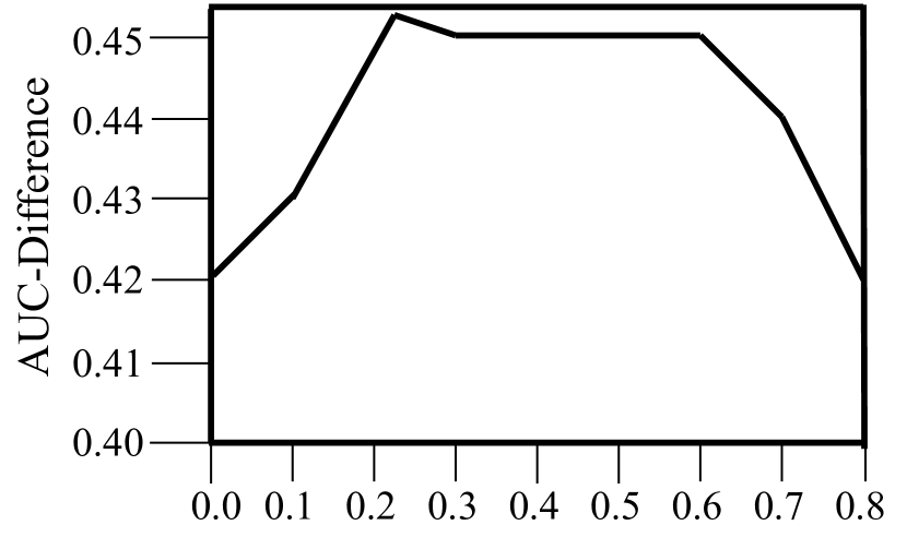
Producing class-specific explanations with DEMUX involves balancing the four key hyperparameters: coefficients for $L_{\text{SSD}}$, $L_{\text{Prev}}$, $L_{\text{Max}}$, and $L_{\text{Budget}}$. We investigate the effects of tuning these coefficients in isolation on the ACSF1 dataset and report our results in Figure 3. For each case, we keep all unchanged parameters at their best-found values.

First, as shown in Figure 3(a), we vary the coefficient $\lambda_{1}$ of $L_{\text{Prev}}$ between 0 to 1. This maintains the prediction probability distribution across all the classes and we find a value of 0.7 suffices. A low value for $\lambda_{1}$ fails to preserve the model’s probability distribution, so the loss function may not encourage instance-specific explanations. There, we notice a gradual increase in AUC-Difference until it stabilizes before dropping for higher values of $\lambda_{1}$. Second, a low value for the coefficient of $L_{\text{Max}}$ $\lambda_{2}$ does not generate good explanations for low probability predictions. Here a high value discards salient time steps from the explanations as shown in Figure 3(b). AUC-Difference increases until $\lambda_{2}$ reaches 0.5 and decreases for values $\geq 0.5$. Third, too-low $L_{\text{Budget}}$ coefficient produces redundant salient time steps, while too high removes important salient time step. AUC-Difference gradually climbs up until this coefficient reaches a value of 0.2, and then it starts decreasing and later stabilizes. The optimal value of 0.2 provides a simple and meaningful explanation as shown in Figure 3(c). Fourth, we vary the coefficients tween 0 to 0.8 and find the optimal value is 0.2 as shown in Figure 3(d). Too low means not enough focus on class-specificity, while a high value could remove important regions in favor of class-specificity.

IV-E6 Case Study on the Meat [34] dataset.

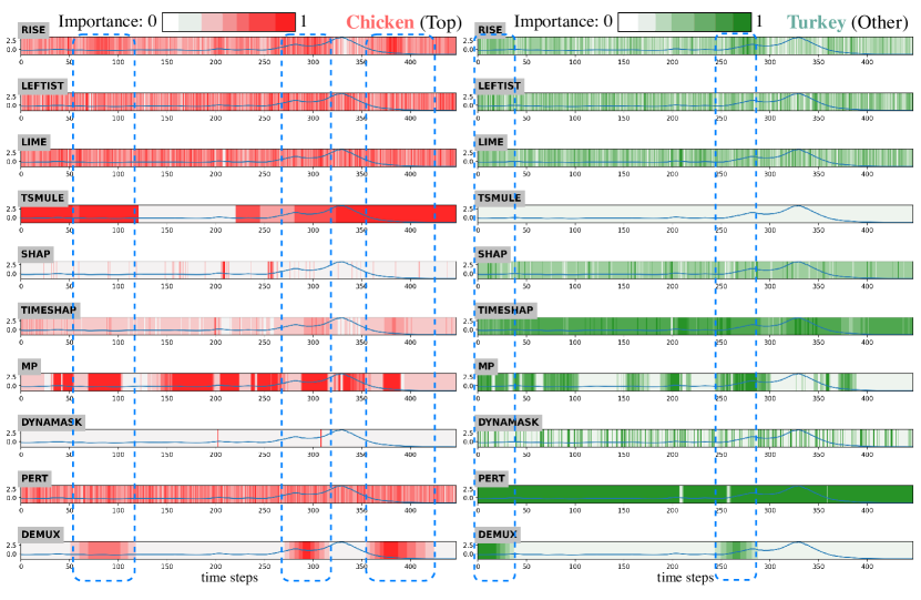
Finally, we describe a case study conducted using DEMUX to explain an RNN’s predictions for an instance from the Meat dataset [34]. Each instance of Meat dataset has 500 time steps. This is a multi-class classification task: Meat is a food spectrograph dataset describing food types as class—a crucial task in food safety and quality assurance. There are three classes: Chicken, Pork, and Turkey, which are predicted with probabilities 88%, 11%, and 1%, respectively for the instance we consider.

Our case study results are shown in Figure 5, where each method’s time step importance is red for class Chicken and green for Turkey, with darker hues indicating higher importance. By visually investigating discriminative subsequences, we see that the compared methods highlight several regions of input time series as important for the top predicted class Chicken. On the contrary, DEMUX (the last row) succeeds to highlight the discriminative subsequences as class-specific evidence for the top predicted class Chicken. Unlike the compared methods, DEMUX has reduced overlapping salient regions between the top predicted class Chicken and class Turkey as shown in the blue dashed vertical boxes (Pork class is not shown due to space constraints). These results suggest that DEMUX’s superiority over state-of-the-art methods is due to the ability to learn class-specific evidence with respect to other classes.

V Conclusion

With this work, we identify class-specificity as a critical criteria for meaningful explanations of multi-class deep time series classifiers. Solving this open problem is essential for users who seek explanations for why a model predicted one class in particular [15]. We introduce DEMUX, the first solution to this open problem, which extends beyond recent methods for perturbation-based explainability for time series models by learning to encourage class-specificity during training via a novel loss function. With three interdependent modules, all of which are learned, DEMUX successfully produces class-specific explanations. In our experiments, we compare DEMUX to nine state-of-the-art explainability methods for two deep models on five multi-class datasets. Our results demonstrate that DEMUX’s explanations are (1) more class-specific than the alternatives, which leads to (2) higher quality according to popular explainability metrics, and (3) consistent explanations across multiple initializations.

References

- [1] M. F. D. et al., “Financial forecasting with -rnns: A time series modeling approach,” in Frontiers in Applied Mathematics and Statistics, 2020.
- [2] B. D. F. et al., “hctsa: A computational framework for automated time-series phenotyping using massive feature extraction.,” Cell systems, 2017.
- [3] Z. Che and et al., “Recurrent neural networks for multivariate time series with missing values,” Scientific Reports, 2018.
- [4] G. L. et al., “Shapenet: A shapelet-neural network approach for multivariate time series classification,” in AAAI, 2021.
- [5] Tonekaboni and et al., “What went wrong and when? instance-wise feature importance for time-series models,” NeurIPS, 2020.
- [6] U. S. et al., “Ts-mule: Local interpretable model-agnostic explanations for time series forecast models,” in PKDD/ECML Workshops, 2021.
- [7] P. S. Parvatharaju, R. Doddaiah, T. Hartvigsen, and E. A. Rundensteiner, “Learning saliency maps to explain deep time series classifiers,” Proceedings of the 30th ACM International Conference on Information & Knowledge Management, 2021.
- [8] J. Crabbe and M. van der Schaar, “Explaining time series predictions with dynamic masks,” in ICML, 2021.
- [9] J. e. a. Bento, “Timeshap: Explaining recurrent models through sequence perturbations,” ArXiv, 2020.
- [10] R. Guidotti and et al., “Explaining any time series classifier,” International Conference on Cognitive Machine Intelligence, 2020.
- [11] M. Guillemé and et al., “Agnostic local explanation for time series classification,” ICTAI, 2019.
- [12] M. T. Ribeiro, S. Singh, and C. Guestrin, “"why should i trust you?": Explaining the predictions of any classifier,” CoRR, 2016.
- [13] L. et.al, “A unified approach to interpreting model predictions,” Advances in Neural Information Processing Systems 30, 2017.
- [14] A. A. Ismail, M. Gunady, H. Bravo, and S. Feizi, “Benchmarking deep learning interpretability in time series predictions,” 2020.
- [15] W. Shimoda and K. Yanai, “Distinct class-specific saliency maps for weakly supervised semantic segmentation,” in ECCV, 2016.
- [16] H. Kaur and et. al, “Interpreting interpretability: Understanding data scientists’ use of interpretability tools for machine learning,” CHI Conference, 2020.
- [17] Ribeiro and et al., “Automatic diagnosis of the 12-lead ecg using a deep neural network,” Nature Communications, 2020.
- [18] F. e. a. Mujkanovic, “timexplain–a framework for explaining the predictions of time series classifiers,” ArXiv, 2020.
- [19] R. Fong and A. Vedaldi, “Interpretable explanations of black boxes by meaningful perturbation,” ICCV, 2017.
- [20] I. Elizabeth and K. et al., “Problems with shapley-value-based explanations as feature importance measures,” in ICML, 2020.
- [21] R. Fong, M. Patrick, and A. Vedaldi, “Understanding deep networks via extremal perturbations and smooth masks,” in ICCV, 2019.
- [22] Omnia and et al., “Deep learning model for financial time series prediction,” International Conference on Innovation in Information Technology, 2020.
- [23] N. Mehdiyev and et al., “Time series classification using deep learning for process planning: A case from the process industry,” Procedia Computer Science, 2017.
- [24] Y. Zhang and et al., “Human activity recognition based on time series analysis using u-net,” ArXiv, 2018.
- [25] U. S and et al., “Towards a rigorous evaluation of xai methods on time series,” CoRR, 2019.
- [26] V. Satopaa and et al., “Finding a "kneedle" in a haystack: Detecting knee points in system behavior,” ICDCS, 2011.
- [27] T. Schaul, J. Quan, I. Antonoglou, and D. Silver, “Prioritized experience replay,” CoRR, vol. abs/1511.05952, 2016.
- [28] V. Petsiuk, A. Das, and K. Saenko, “Rise: Randomized input sampling for explanation of black-box models,” CoRR, vol. abs/1806.07421, 2018.
- [29] Gisler and et al., “Appliance consumption signature database and recognition test protocols,” in WoSSPA, 2013.
- [30] Y. Chen, E. Keogh, B. Hu, N. Begum, A. Bagnall, A. Mueen, and G. Batista, “The ucr time series classification archive,” 2015. www.cs.ucr.edu/~eamonn/time_series_data/.
- [31] D. Roverso, “Multivariate temporal classification by windowed wavelet decomposition and recurrent neural networks,” 2000.
- [32] A. Baldridge, S. Hook, C. Grove, and G. Rivera, “The aster spectral library version 2.0,” Remote Sensing of Environment, 2009.
- [33] A. L. Goldberger and et al., “Physiobank, physiotoolkit, and physionet: components of a new research resource for complex physiologic signals.,” Circulation, 2000.
- [34] O. Al-Jowder, E. Kemsley, and R. Wilson, “Mid-infrared spectroscopy and authenticity problems in selected meats,” Food Chemistry, 1997.
- [35] Z. Wang and et al., “Time series classification from scratch with deep neural networks: A strong baseline,” IJCNN, 2017.
- [36] A. Charnes and et al., “Extremal principle solutions of games in characteristic function form: Core, chebychev and shapley value generalizations,” Springer Netherlands, 1988.
- [37] D. P. Kingma and J. Ba, “Adam: A method for stochastic optimization,” CoRR, vol. abs/1412.6980, 2015.
- [38] L. Biewald, “Experiment tracking with weights and biases,” 2020. Software available from wandb.com.
- [39] N. Hama, M. Mase, and A. B. Owen, “Deletion and insertion tests in regression models,” 2022.