Analysis of Expected Hitting Time for Designing Evolutionary Neural Architecture Search Algorithms

Abstract

Evolutionary computation-based neural architecture search (ENAS) is a popular technique for automating architecture design of deep neural networks. In recent years, various ENAS algorithms have been proposed and shown promising performance on diverse real-world applications. In contrast to these groundbreaking applications, there is no theoretical guideline for assigning a reasonable running time (mainly affected by the generation number, population size, and evolution operator) given both the anticipated performance and acceptable computation budget on ENAS problems. The expected hitting time (EHT), which refers to the average generations, is considered to analyze the running time of ENAS algorithms. This paper proposes a general framework for estimating the EHT of ENAS algorithms, which includes common configuration, search space partition, transition probability estimation, and hitting time analysis. By exploiting the proposed framework, we consider the so-called ($\lambda$+$\lambda$)-ENAS algorithms with different mutation operators and manage to estimate the lower bounds of the EHT which are critical for the algorithm to find the global optimum. Furthermore, we study the theoretical results on the NAS-Bench-101 architecture searching problem, and the results show that the one-bit mutation with “bit-based fair mutation” strategy needs less time than the “offspring-based fair mutation” strategy, and the bitwise mutation operator needs less time than the $q$-bit mutation operator. To the best of our knowledge, this is the first work focusing on the theory of ENAS, and the above observation will be substantially helpful in designing efficient ENAS algorithms.

I Introduction

Manually designed convolutional neural networks (CNNs) [1, 2, 3, 4, 5] have been showing their promising performance in diverse real-world applications [6], such as image classification [7], natural language processing [8] and speech recognition[9], to name a few. The architectures of these state of the art demand rich expertise from their designers in both CNNs and domain knowledge of the problems to be solved. This has motivated researchers to comprehensively conduct neural architecture search (NAS) that can automatically design promising CNN architectures. In practice, NAS is typically modeled as an optimization problem that is often non-convex and non-differentiable [10]. The optimization algorithms primarily employed to address NAS can be classified into three different categories: reinforcement learning (RL), gradient descend, and evolutionary computation (EC). The RL-based NAS algorithms [11, 12] often consume thousands of GPU days even searching for the optimal architectures on median-scale datasets. The gradient descend-based NAS algorithms [13, 14, 15] are more efficient than the RL-based algorithms, but they require constructing a supernet in advance, which also needs expertise intervention. The EC-based NAS (ENAS) algorithms [16], which generally require fewer computational resources than RL-based ones and can also fully automate CNN architecture search, are widely used in the NAS field. Specifically, the EC is a family of heuristic algorithms that simulate the evolution of species or the behaviors of the population in nature, and the evolutionary algorithms (EAs) and swarm intelligence are the popular EC methods. In fact, EC had been widely used to design neural network architectures decades ago, of which a comprehensive survey can be checked from [17]. Furthermore, despite a difficult period in neural network research from the mid-1990s to 2006, there were still some well-known methods that used EC to optimize neural network architectures, such as NEAT [18] and its variants, HyperNEAT [19] and ES-HyperNEAT [20]. In 2017, Google company took the initial step in proposing an ENAS algorithm especially for CNNs [21]. Since then, a slew of excellent ENAS algorithms have been proposed [22, 23, 24, 25], showing superior performance mainly in image classifications.

Despite their success, ENAS also faces some issues stemming from their wide application in practice. For example, the performance of an EC-based algorithm often positively relies on the number of fitness evaluations (running time) decided by the settings of population size and generation number (iterations). In general, the more iterations there are, the more architectures will be evaluated, and the better performance obtained. In some computation economy optimization problems, the most common practice is to specify a large generation number and population size that collectively result in a huge volume of running time to guarantee the better performance. However, NAS is a prohibitively expensive problem because numerous deep neural architectures will be trained during the search. In general, the training of one deep architecture will consume hours to days even run on GPU cards for medium-scale datasets. Due to the population nature of EC, the computation cost of ENAS becomes unacceptable. For instance, the large-scale evolution method [21] used 250 GPUs for 11 days, the AmoebaNet [23] costed 450 GPUs for 7 days. However, such immense computation resources are not necessarily available to every researcher interested. One question is naturally raised: if could we assign a reasonable running time to ENAS algorithms in advance so that they would not take unnecessary computation budget during the search yet can still achieve promising performance? The answer involves the theoretical study on the running time, which is a core theoretical issue.

In the recent decade, EC running time analysis has been minimally touched. Even so, most earlier studies consider EAs with only a single parent or offspring (i.e., (1+1)-EA or ($\lambda$+1)-EA) [26, 27, 28, 29, 30, 31], and rarely consider population-based EAs (such as ($\lambda$+$\lambda$)-EA, a specific version of ($\mu$+$\lambda$)-EA with $\mu=\lambda$), while the latter EAs are widely used in ENAS for optimizing the search. The existing population-based studies [32, 33, 34, 35, 36] are more concerned with EAs solving specific test problems which cover the P and NP-hard combinatorial problems, such as the LEADINGONES problem[37], the ONEMAX problem[38], the TRAPZEROS problem[34], and so on. In these traditional optimization problems, the variables are often in the Euclidean space, which allows the problem expressed as pseudo-Boolean function, whereas ENAS is a problem in which the variables refer to deep architectures of more sophisticated data and cannot be expressed in an explicit form. Moreover, most previous running time analyses on population-based EAs only showed upper bounds, which are helpful for revealing the ability of the algorithm. However, the analysis of the lower bounds, which reveal the limitation, is equally critical for understanding the algorithm complexity. Therefore, it is necessary to build a theoretical framework suitable for analyzing the running time of population-based ENAS algorithms. Based on this, the lower bound can be calculated and the researchers can understand the effects of parameters and operator as well as make comparisons between different algorithms.

The running time of EAs has been widely investigated under the umbrella of expected hitting time (EHT) which is the average generation number required to find an optimal solution[39]. There are many literatures devoted to the analysis approaches [40, 41]. Among those, the best-known representatives are the fitness-level method [42, 43, 44, 45], the convergence-based method [46], and the drift analysis method [47, 48, 49, 50]. The first one, the fitness-level method, partitions the solution space into level sets according to fitness values, and then the level sets are ordered according to the fitness of solutions in the sets. After that, the bound of the EHT can be estimated by the probability of leaving each level set. However, the space is hard to find a useful partition for complex fitness functions that widely exist in real-world applications. The second one, the convergence-based method, applies convergence to imply how close the current state is to the target state at each step, and thus estimates the probability of EAs jumping into the optimal solution in one step (called success transition probability). The bound of the EHT can be estimated by the bound of the success transition probability. However, the transition probability is treated the same for all solutions, which makes it not flexible. The last one, the drift analysis method, is the most widely used method because of its intuitive nature and wide applicability. It measures the length of the whole path toward the optimum and the length of the progress of the EA at each step (called step drift), and then the bound of EHT can be estimated by dividing the path length by the step drift. Researchers have proposed a variety of universal variants to analyze the EHT of EAs, such as combining the takeover time concept and drift analysis [32], average drift analysis [39], just to name a few [51]. However, designing such an appropriate measurement lacks general guidelines and is also problem-dependent.

The current work presents a framework which transforms drift analysis into an ENAS applicable analyzing method. As expected, the following issues need to be considered: 1) How to bridge the gap of modeling ENAS algorithms by Markov chains? 2) How to identify a suitable distance function (also called drift function or potential drift) that is extremely helpful to analyze one step of change (also called progress)? 3) How to design transition probability analysis methods to calculate the one-step change of the distance?

Based on the above discussion, this paper establishes a systematical analytical framework for analyzing the EHT of the ENAS algorithms for the first time, and further explores the effects of various operators and parameters on the EHT. The contributions of our work can be summarized as follows.

1. We define a combination encoding schema as common configuration to bridge the gap in modeling ENAS algorithms by the Markov chains. This work solves the problem that the variables (deep architecture) in the ENAS algorithm are not Euclidean data and thus is hard to study further using binary encoding used in most EA theoretical analyses.

2. By defining the partition method of the search space based on Hamming distance, we develop five proven conclusions for appropriately investigating the mutation transition probabilities and calculating one step of change. This work lays the groundwork for further theoretical investigation and provides a reference for other EAs scenarios.

3. Based on the proposed systematical framework, we employ the so-called ($\lambda$+$\lambda$)-ENAS algorithms with the one-bit, $q$-bit, and bitwise mutation operators and derive four theorems about the lower bounds of the EHT. These findings demonstrate the effectiveness of our analytical framework.

4. We utilize the NAS-Bench-101 architecture searching problem[52] in case studies and gain insight toward the relationship between some algorithmic features and problem characteristics. This allows our work to move closer to our ultimate goal of guiding the design of new ENAS algorithms in practice using theoretical insight.

The rest of the paper is organized as follows. In Section II, we introduce the ENAS algorithm and some theoretical analysis tools. In Section III, we introduce the proposed analytical framework in detail, including the common configuration of the ENAS algorithm, the transition probability analysis, and so on. Section IV investigates the lower bounds of the EHT for ($\lambda$+$\lambda$)-ENAS algorithms using various mutation operators. In Section V, we present the case studies about our theory approach. Section VI concludes this paper along with highlighted future research directions.

II Preliminaries

In this section, we introduce the NAS problem and present the main steps of the ($\lambda$+$\lambda$)-ENAS algorithms based on EAs considered in this paper. Afterwards, the popular tools available for theoretically analyzing EAs are elaborated.

II-A Problem and Mutation-Based ENAS Algorithms

We can mathematically express the NAS problem as an optimization problem and formulate as

$$\mathop{\arg\max}_{A\in\mathcal{A}}\mathcal{L}(A,\mathcal{D}_{\rm test})$$ (1)

where $A$ denotes a CNN architecture, $\mathcal{L}(\cdot)$ measures the performance of the $A$ on the test data set $\mathcal{D}_{\rm test}$, $\mathcal{A}$ denotes the search space, and $\mathcal{L}(\cdot)$ represents the fitness value. There are several challenges to solve this complex optimization problem, e.g., constraints, discrete representations, bi-level structures, computationally expensive characteristics [16].

The algorithm that exploits EA to solve the above NAS problem is called ENAS algorithm. A general EA is the ($\mu$+$\lambda$)-EA, which creates $\lambda$ offspring individuals in each generation and chooses the best $\mu$ individuals from the offsprings and parents to survive for the next generation. There have been various implementations of EAs that may result in different theoretical observations. Without loss of generality, in this work, we focus on the ($\lambda$+$\lambda$)-ENAS algorithms , i.e., the neural architecture search algorithm based on ($\lambda$+$\lambda$)-EA that is a general-purpose EA with a mutation only. Please note that this also follows the conventions of the community [32, 33, 34].

The main steps of a typical ($\lambda$+$\lambda$)-ENAS algorithm are described as follows. Given the randomly initialized parent population $P$, the algorithm repeatedly generates an offspring population $Q$ and then selects a new population serving as the parent population for the next generation, until the predefined maximal generation number is reached. In each generation, the offspring population $Q$ with size $|P|$ is generated by mutation operation upon the individuals in $P$, and then the new population with the size of $|P|$ is selected given $P$ and $Q$ together by an elitist selection operation. When the stopping criterion is met, the algorithm stops the above iterative procedures, selects the optimal individual $p^{*}$ from the current population $P$, and decodes $p^{*}$ into the corresponding deep neural network as the resulting output. In this paper, we only consider the ENAS algorithms following mutation and selection operators.

• One-bit mutation: Randomly flip one bit of each solution.

• q-bit mutation: Randomly flip $q$ bits of each solution.

• Bitwise mutation: Independently flip each bit of each solution with uniform probability $p_{m}$, where $p_{m}$ is called the mutation rate. In this paper, we consider a commonly used mutation rate, i.e., $p_{m}=1/n$ [53], where $n$ is the length of the solution.

• Truncation selection: Sort $2\lambda$ individuals by their fitness in the descending order, then, select $\lambda$ best individuals as the next generations [32].

• Non-repeated selection mechanism: Randomly select individuals one by one without repetition.

II-B Markov Chain Modeling

Definition 1 (Markov Chain)

A Markov Chain is a sequence of random variables $\left\{{\xi_{t}}\right\}_{t=0}^{+\infty}$ whose state is defined in a finitely space, and satisfies the following formula:

$$\forall t\geq 0:P(\xi_{t+1}|\xi_{t},\xi_{t-1},\ldots,\xi_{0})=P(\xi_{t+1}|\xi_{t}).$$

EAs evolve solutions from generation to generation, where the state of the next generation depends on the previous one. Obviously, it can be seen from Definition 1 that the Markov chain has the characteristic of “memorylessness”, which means that the state at the next time is independent of all previous states. As a result, EAs were always naturally modeled by Markov chains [54]. Based on this fact, the ENAS algorithm, which is an extension of EA, can also be modeled by the Markov chain. For clarity, the mapping of the core components of EAs and the Markov chains are shown in Table I. Particularly, a multiset with $\lambda$ solutions or individuals corresponds to a population, whereas an individual $s$ in the EA corresponds to a CNN architecture in the ENAS algorithm. When the population size $\lambda$ is one, the state space of the Markov chain corresponds to the solution space $S$; otherwise, it corresponds to the population space $\chi$. We call a population optimal if it contains at least one optimal solution, and the subspace composed of the optimal population is called target state space $\chi^{*}$.

TABLE I: The mapping between core components of EA and Markov chain used in this study.

Notations	EA	Markov Chain
$s$	Solution / Individual	State
${\xi_{t}}$	Population
$S$	Individual Space	State Space
${\chi}$	Population Space
$\chi^{*}$	Target Population Space	Target State Space
$T$	Expected Generation Number	Expected Hitting Time

Let $\{{\xi_{t}}\}_{t=0}^{+\infty}$ be the Markov chain associated with an EA. Its first hitting time which is used to measure the time complexity of EAs starting with the initial state $\xi_{0}$ is defined by

$$T=\min\{t\geq 0;\xi_{t}\in\chi^{*}|\xi_{0}\}.$$

The expected first hitting time (EHT) of the absorbing Markov chain can then be represented by

$${E}[T]=\sum_{t=0}^{+\infty}P(\xi_{t}\in\chi-\chi^{*}).$$

The ENAS algorithm aims to search the optimal population $\xi_{T}\in\chi^{*}$ starting from the initial random population $\xi_{0}$, while $T$ is the expected generation number of an ENAS algorithm. Since the process of ENAS can be described as a Markov chain, the $T$ corresponds to the EHT of the Markov chain. It is worth noting that EHT represents the average number of generations rather than the best or worst generations for an ENAS algorithm before producing the final solution [55].

II-C The Drift Analysis Approach

Drift analysis is a powerful tool for measuring the one step change of the potential (also called drift function or distance function) and is further used to calculate the runtime of an algorithm when it reaches its goal. In this paper, we use the drift analysis to estimate the EHT of the ENAS algorithms. Usually, there are three steps [50]: 1) identify a distance function $d(\cdot,\cdot)$ that measures the disparity between population and the optimal point; 2) represent the one-step change of drift which is also named point-wise drift; 3) use a specific drift analysis method to translate the point-wise drift into information about the number of steps until the algorithm has achieved the goal, i.e., EHT.

Specifically, we use $d(X,\chi^{*})=\min\{d(X,S^{*}):S^{*}\in\chi^{*}\}$ as the distance between the population $X$ and the target population space $\chi^{*}$. In short, we denote the distance by $d(X)$ and it satisfies $d(S^{*})=0,S^{*}\in\chi^{*}$. Then, the drift of random sequence $\{d(\xi_{t});t=0,1,\dots\}$ is defined by

$$\Delta(d(\xi_{t}))=d(\xi_{t})-d(\xi_{t+1}).\vspace{-0.6em}$$

Furthermore, given any concrete $X\in\chi-\chi^{*}$ as $\xi_{t}$ at generation $t$, the point-wise drift can be obtained by

$$\Delta(X)=\mathbb{E}[d(\xi_{t})-d(\xi_{t+1})|\xi_{t}=X].\vspace{-0.6em}$$

Due to evolutionary randomness, the next generation population $Y\in\chi$ as $\xi_{t+1}$ conforms to certain random progress. Therefore, we can further describe point-wise drift as the expected drift or average drift which is first used in [56] and is given by

$$\bar{\Delta}_{t}=\mathbb{E}[\mathbb{E}[d(\xi_{t})-d(\xi_{t+1})|\xi_{t}=X]\mid X\in\chi-\chi^{*}].\vspace{-0.6em}$$

Lastly, we present the stopping time of EAs, i.e., EHT. Assume that the distance between the initial population and optimal point is $d(\xi_{0})$, if the drift toward the optimal point is greater than the represented $\Delta$, the algorithm needs at least $d/\Delta$ iterations (i.e., generations) in expectation to search for the optimal point. The average drift theorem [39] proposed an approach to estimate the lower and upper bounds of EHT, as shown in Lemma 2. It can be seen that the key issue here is to estimate $\Delta$ and $d(\xi_{0})$ (corresponding the $\bar{\Delta}_{t}$ and $\mathbb{E}[d(\xi_{0})]$).

Lemma 1

[39] Given a Markov chain $\left\{{\xi_{t}}\right\}_{t=0}^{+\infty}$ converges to $\chi^{*}$ where initial state $\xi_{0}$ satisfies $P(\xi_{0}\in\chi-\chi^{*})>0$, and there is an initial distance $d(\xi_{0})$. For each generation $t$, there is an average drift $\bar{\Delta}_{t}$. If there is $0<c_{2}\leq\bar{\Delta}_{t}\leq c_{1}$, where both $c_{1}$ and $c_{2}$ are greater than 0, then the EHT satisfies:

$$\frac{\mathbb{E}[d(\xi_{0})]}{c_{1}}\leq\mathbb{E}[T]\leq\frac{\mathbb{E}[d(\xi_{0})]}{c_{2}}.\vspace{-1em}$$ (2)

This drift analysis approach can be straightforwardly used to analyze EHT for classical optimization problems but not for ENAS problems as discussed above. Specifically, the encoding issues caused by the complex solution structure, as well as issues such as probability analysis and search space partition involved in the drift calculation process, have hindered us from directly using the above method to analyze the EHT.

III The Analytical Framework

This section proposes the theoretical analytical framework for calculating the mean number of generations (EHT) of ENAS algorithms. Through this framework, we aim to provide researchers with some proven approaches and justifiable findings in analyzing the time complexity of ENAS, and inspire researchers in the field of ENAS to carry out further work on runtime analysis based on this. The details of the proposed framework, in short, named CEHT-ENAS, are shown in Algorithm 1. Particularly, CEHT-ENAS is composed of four parts: common configuration (line 2-4), search space partition (lines 6), transition probability estimation (lines 8-13), and hitting time analysis (lines 15-19).

• Common Configuration: We propose a genetic encoding approach tailored specifically for CNN architectures in ENAS algorithms. This will bridge the gap in modeling ENAS algorithms by the Markov chain.

• Search Space Partition: We define the distance measurement function for the current state space to the target state space. Based on this, the search space can be reasonably partitioned, and the subsequent transition probability can be accurately estimated. In this subsection, we give two methods of search space partition.

• Transition Probability Estimation: We develop lemmas for calculating the transition probability between two states in algorithms with different encoding methods and mutation operators. These servers as the foundation for performing the drift analysis.

• The Hitting Time Analysis: We elaborate the formulas for calculating the point-wise drift, average drift and the expected initial distance before calculating the EHT of ENAS algorithms.

In the following, we will document and justify the design of these parts.

Algorithm 1 The Framework of CEHT-ENAS

Input: ENAS algorithm
Output: $\mathbf{EHT}$

1:  Common configuration phase:

2:      $\{v,L,\lambda\}$ $\leftarrow$ Load the search space parameters;

3:      $\{n,n_{1},n_{2},S,\chi\}$ $\leftarrow$ Configure the ENAS algorithm;

4:      $\left\{{\xi_{t}}\right\}_{t=0}^{+\infty}$ $\leftarrow$ Model ENAS algorithm as Markov chain;

5:  Search space partition phase:

6:      $\left\{{\chi_{i}}\right\}_{i=0}^{n}$ $\leftarrow$ Partition the search space into multiple subspaces;

7:  Transition probabilities estimation phase:

8:      $P^{m}(X,Y)$ $\leftarrow$ Estimate the mutation transition probability from $X$ to $Y$;

9:         if one-bit mutation then $P^{m}_{1}(X,Y)$ or $P^{m}_{2}(X,Y)$;

10:         if q-bit mutation then $P^{m}_{3}(X,Y)$;

11:         if bitwise mutation then $P^{m}_{4}(X,Y)$;

12:      $P^{s}(X,Y,Z)$ $\leftarrow$ Estimate the probability of selecting individuals from $X\cup Y$ based on selection operation;

13:      $P(X,Z)$ $\leftarrow$ Estimate the transition probability between two neighbour generations;

14:  The hitting time analysis phase:

15:      $\Delta(X)$ $\leftarrow$ Estimate the point-wise drift of solution $X$;

16:      $\bar{\Delta}_{t}$ $\leftarrow$ Estimate the average drift at the $t$-th generation;

17:      $P\left(\xi_{0}=X\right)$ $\leftarrow$ Estimate the probability when the state $\xi_{0}$ equals to a state $X$ in the non-target state space;

18:      $\mathbb{E}[d(\xi_{0})]$ $\leftarrow$ Calculate the expected distance of the initial solution $x_{0}$.

19:  return $\mathbb{E}[T]$ $\leftarrow$ $\mathbb{E}[d({\xi}_{0})]/\bar{\Delta}_{t}$

III-A Common Configuration of ENAS Algorithms

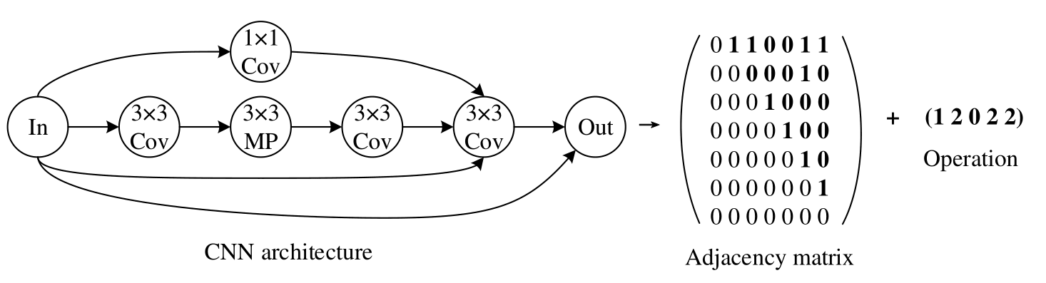
Figure 1: The architecture and encoding schematic of CNN.

In the traditional optimization problems, the variables are often in the Euclidean space, which is in turn easily represented by binary strings, and then investigated by existing analysis tools. However, in the ENAS algorithms which cannot be regarded as Euclidean data, the variables refer to deep architectures which are not Euclidean data. Particularly, one deep architecture is always composed of two parts, one of which is to display the connections information of deep network architecture, while the other is to display operations information of the network nodes. This makes it hard to study further using binary encoding for the following reasons. The one-hot encoding, as the binary string encoding method is used in the ENAS community, two misgivings with this method make it unrealistic to use for theoretical analysis of the variation between solutions. First, the general binary encoding method makes the difference between any two different node operations more than one (e.g., $0010$ represents the 3$\times$3 convolution operation, $0100$ represents the 3$\times$3 maxpool operation, and there are two bits that differ), so that for a successful conversion between two operations it must mutate more than one bit to succeed, thus, it further leads to the zero probability of conversion between operations. Furthermore, it will further lead to the feared result that some node operations will never appear in candidate solutions by mutating (with the involvement of the selection operator). Second, the binary encoding method causes the size of solution encoding to grow exponentially as the nodes number and operations type number increase which is both defined in the DNN architecture search space, while the excessive encoding size is not sensible for theoretical analysis. As a result, the binary string encoding method cannot be directly used.

In principle, any deep architecture can be formulated by directed cyclic graphs, where the edges and the nodes of the graph correspond to the connections and operations of the deep architecture. Motivated by this, in this work, we propose a combination genetic encoding method based on real numbers elaborately for ENAS in terms of its graph representation, which is composed of two parts. The first is the representation of the edges which is composed of the upper triangular matrix, where “1” represents an edge. The second is composed of a string of real numbers $\left\{0,1,\ldots,L\right\}$, where $L+1$ is the number of operation types of one node. For the sake of clarity, we explain the above using CNN as an example. As shown in Fig. 1, the network architecture contains seven nodes (in, out, and five internal nodes) and nine edges, where each internal node represents one of the three operations (3$\times$3 convolution,1$\times$1 convolution, and 3$\times$3 maxpool, i.e., $L=2$). Since the architecture is a directed acyclic graph, the elements of the 7$\times$7 upper triangular adjacency matrix composed of 7 points describe the network connections. As a result, there are 21 possible edges, which correspond to the length of the first encoding part. Similarly, the number 5 of the internal nodes corresponds to the length of the second encoding part, and the number of operations minus one corresponds to $L$.

To make the analysis framework more general to ENAS algorithms, the following common configuration is presented:

• Parameter: $v$ represents the maximum number of nodes in the search space of the network architectures, $n_{1}=v(v-1)/2$ represents the number of possible edges in the upper triangular matrix, $n_{2}=v-2$ refers to the number of intermediate vertices except the input and output vertices, $n=n_{1}+n_{2}$ refers to the individual length, and $\lambda$ specifies the population size.

• Encoding: Solution $s$ is encoded by combining string $a\in\{0,1\}^{n_{1}}$ and string $b\in\{0,1,\ldots,L\}^{n_{2}}$, e.g.,

  $s=(\underbrace{110011000101000100101}_{a=\{0,1\}^{21}}\circ\underbrace{12012}_{b=\{0,1,2\}^{5}})$

• Solution space: $S={\{0,1\}}^{n_{1}}{\{0,1,\ldots,L\}}^{n_{2}}$, and its size is $|S|=2^{n_{1}}(L+1)^{n_{2}}$.

• Population space: $\chi={\{\{0,1\}}^{n_{1}}{\{0,1,\ldots,L\}}^{n_{2}}\}^{\lambda}$, the population is considered as an disordered and repeatable set of solutions, so its size is $|\chi|={\lambda+|S|-1\choose\lambda}$.

• Initialization: Randomly generate a population of $\lambda$ solutions encoded by the above encoding method.

• Fitness: The fitness of solution $s$ is defined as $f(s)$; the fitness of population $X$ is defined as the maximal fitness of its individuals, i.e., $f(X)=\max\{f(s):s\in X\}$.

• Optimal solution: For simplicity, we assume that the solution $s^{*}$ with the highest fitness value is unique.

• Distance: The distance of solution $s$ to optimal solution is defined as $d(s)$; the distance of population $X$ is defined as the minimal distance of its individuals, i.e., $d(X)=\min\left\{d(s):s\in X\right\}$, which measures the distance from $X$ to the target population space $\chi^{*}$.

• Stopping criterion: The algorithm halts once $s^{*}$ is found.

According to the proposed encoding method, we further update the calculation of the number of solutions for each distance class in solution space $S$. First, for using the traditional individual encoding method $\{0,1\}^{n}$, we can obviously get that there are $n\choose d$ individuals belonging to the class with distance $d$ in $S$. But for the proposed combination encoding $\{0,1\}^{n_{1}}\{0,1,...,L\}^{n_{2}}$, we need further divide an encoding of one solution into two parts, and their distance values are denoted as $d_{1}$ and $d_{2}$, where $d_{1}+d_{2}=d$. And then, we can express that the number of individuals with distance $d$ in $S$ is $C(d)$, as shown in formula Eq.(3).

$$C(d) =\left\{\begin{aligned} &\leavevmode\resizebox{10.0pt}{}{ $\sum_{d_{1}=0}^{d}{L^{d_{2}}{n_{1}\choose d_{1}}{n_{2}\choose{d_{2}}}},$ }&d<n_{1};\\ &\leavevmode\resizebox{10.0pt}{}{ $\sum_{d_{1}=\max\{d-n+n_{1},0\}}^{n_{1}}L^{d_{2}}{n_{1}\choose d_{1}}{n_{2}\choose{d_{2}}},$ }&d\geq n_{1}.\end{aligned}\right.$$ (3)

In order to address the distinct mutation requirements brought on by the complexity encoding of deep architecture, we define two new mutation strategies, bit-based fair mutation, and offspring-based fair mutation. The former strategy ensures that each bit is chosen with an equal probability, and the latter strategy ensures that each potential offspring has an equal chance of being born. For individuals using the binary encoding mechanism, both types of strategies can ensure that the mutation operator flips each bit fairly, and can also guarantee that each offspring has the same probability of being born. However, for the ENAS algorithm that can not utilize the binary encoding mechanism and must use the proposed combination encoding mechanism, if the “bit-based fair mutation” strategy is used, the chance of each possible offspring been generated varies, because the non-binary encoding part must consider which new bit (i.e., the number between 0 and $L$ except for itself) is mutated to rather than simply flipping the bit from 0 to 1 (or 1 to 0) as binary encoding does. As a result, in addition to the so-called “unfairness” in this scenario, we analyze the circumstance when the algorithm utilizes the “offspring-based fair mutation” strategy in the theoretical analysis. Based on the two strategies defined above, the following mutation operators will be considered.

• Mutation#1 (One-bit mutation with “bit-based fair mutation” strategy): For each individual $x$, uniformly select an integer $r\in[1,n]$, and then mutate the $r$-th bit. In this case, if $r\in(n_{1},n]$, it needs to additionally select an integer $l\in[0,L]\setminus\{x_{r}\}$ randomly, where $x_{r}$ represents the value of the $r$-th bit. Although each bit in non-binary encoding individual is fairly selected, each possible offspring birth is unfair. This is due to the fact that each bit in the non-binary encoding part can produce $L$ times more variants than the binary encoding part.

• Mutation#2 (One-bit mutation with “offspring-based fair mutation” strategy): For each individual, randomly select an integer number $r\in[1,n_{1}+Ln_{2}]$ with probability $1/(n_{1}+Ln_{2})$. If $r\in[1,n_{1}]$, then flip the $r$-th bit; else mutate the $(n_{1}+\lceil\frac{r-n_{1}}{L}\rceil)$-th bit into one of the number from $[0,L]\setminus\{x_{i}\}$, where ${x_{i}}$ represents the encoding value corresponding to the $(n_{1}+\lceil\frac{r-n_{1}}{L}\rceil)$-th bit of individual $x$. In this way, the probability of selecting any bit belonging to the first $n_{1}$ bits is $1/(n_{1}+Ln_{2})$, which is less than the probability of selecting from the last $n_{2}$ bits, i.e., $L/(n_{1}+Ln_{2})$. This mutation strategy ensures that individuals who cannot use the binary encoding method can mutate fairly, that is, each sub-generation has the same chance of being generated. This is not guaranteed by the traditional Mutation#1.

• Mutation#3 (q-bit mutation with “bit-based fair mutation” strategy): For each individual, randomly select $q$ unique integers $\{q_{i}\}_{i=1}^{n}$ with probability $1/{n\choose q}$, where $q_{i}\in(0,n]$, and then mutate the $q$ bits. The mutation operation of each bit is similar to Mutation$\#1$.

• Mutation#4 (bitwise mutation): For each individual, independently mutate each bit with probability $p_{m}=1/n$.

III-B Search Space Partition

The transition probability is the key to theoretically investigating ENAS algorithms because it is the basis for understanding how the initial population progresses to the target population. In order to facilitate the analysis of transition probability, we intend to partition the search space into several subspaces according to some bases, e.g., fitness, distance, and so on. In the following, we first discuss the definition of the distance function, and then we consider the basis for partitioning the search space from two distinct aspects.

In ENAS algorithms, the structure of a solution would be changed after one evolution operation, and the corresponding fitness may also be varied accordingly. Through experiments, the difference between the fitness values, of which the solution with and without mutation, can be directly obtained as the distance values. This is in contrast to the situation of theoretical analysis, how to express the progress (distance) of two solutions is very challenging. This is because it involves the encoding and fitness function representation, which makes it requires particular analysis of specific issues. According to the encoding method of the solution, we find that the encoding differences caused by mutation operation can be represented by the Hamming distance. In this paper, we use the Hamming Distance shown in Definition 2 to measure how far an individual $s$ is away from the optimal point $s^{*}$, that is, the distance $d(s)$. And the distance function for population is denoted as $d(X)=\min\left\{d(s):s\in X\right\}$.

Definition 2 (Hamming Distance)

Given two strings of equal length, $s_{1}$ and $s_{2}$, the number of positions with different symbols corresponding to the two strings is the Hamming distance, which is represented by

$$H(s_{1},s_{2})=\sum_{i=1}^{n}I(s_{1}[i]\neq s_{2}[i]),\vspace{-0.6em}$$

where $I(\cdot)$ is the indicator function that is 1 if the inner expression is true and 0 otherwise, $s_{1}[i]$ and $s_{2}[i]$ represent the $i$-th bit of individuals $s_{1}$ and $s_{2}$, respectively.

Then, we discuss the basis for partitioning the search space. From the perspective of utilizing fitness value as the criterion to divide search space, we can directly define the optimal subspaces and the non-optimal subspaces. But for millions of solutions that often exist in an ENAS algorithm, we cannot exactly know how much the fitness value has changed after the individual has performed the mutation operation, and we cannot divide the search space with such vanilla approaches. Therefore, we consider the distance as the space partition. From the perspective of individuals, the search space which is also called solution space $S$, is a set of real number strings. According to the distance value, we divide the solution space $S$ into $(n+1)$ subspaces without overlaps, i.e., $\{S^{i}\}^{n}_{i=0},\forall i\neq j,S^{i}\cap S^{j}=\emptyset$. The distance values of all solutions in $S^{i}$ are $i$. For population space $\chi$, we partition it into $(n+1)$ subspaces $\{\chi_{i}\}^{n}_{i=0}$, where the subspace $\chi_{0}$ equals to $\chi^{*}$ that contains all the optimal populations (the distance of the optimal solution in the population is zero). All populations in the subspace $\chi_{i}(i\in\left\{1,2,\ldots,n\right\})$ are non-optimal solutions, and the minimum distance value of the solutions in each population is $i$. Based on the previous method, space $\chi_{i}$ can be subdivided into $\lambda$ small subspaces, i.e., $\{\chi_{i}^{\gamma}\}^{n}_{i=1}(\gamma=1,2,\dots,\lambda)$, where $\gamma$ represents the number of individuals of which distance values are $i$. Then, there are $\lambda(n+1)$ subspaces. Therefore, the size of subspace $\chi_{i}$ can be denoted by $|\chi_{i}|=\sum_{\gamma=1}^{\lambda}|\chi_{i}^{\gamma}|$, where

and $C(i)$ as in Eq.(3) is the number of solutions with distance $i$.

With these designs, we can make it easier to analyze the transition probability of the states in the two subspaces, which will be introduced next.

III-C Transition Probability

How to represent the transition probability is the key to analyzing the progress of ENAS algorithms in each step and calculating the point-wise drift. To the best of our knowledge, there is no specific approach to transition probability calculation. In this part, we provide several lemmas to enable the investigation of the transition probability. These findings are applicable to analyze the other EC scenarios using the combination encoding mechanisms and provide insights for further studying evolution operators.

Generally, each generation of ENAS consists of two steps: generating new individuals by evolution operation and selecting the individuals surviving into the next generation. For the convenience of the discussion, this process at the $t$-th generation is formulated as:

where the transition probability from $\xi_{t}$ to $\xi^{m}_{t}$ is expressed by using mutation transition probability:

$$P^{m}(X,Y)\overset{def}{=}P(\xi^{m}_{t}=Y|\xi_{t}=X),X\in\chi-\chi^{*},Y\in\chi;$$

while the transition probability from population $\xi_{t}\cup\xi^{m}_{t}$ to $\xi_{t+1}$ is represented by:

$$P^{s}(X,Y,Z)\overset{def}{=}P(\xi_{t+1}=Z|\xi_{t}=X,\xi^{m}_{t}=Y),Z\in\chi;$$

the transition probability from $\xi_{t}$ to $\xi_{t+1}$ is represented by:

$$P(X,Z)\overset{def}{=}P(\xi_{t+1}=Z|\xi_{t}=X).$$

Please note that the formula of transition probability does not change with the transformation in $t$, because there is no self-adaptive strategy employed by EAs.

Since the analysis of population evolution relies on individuals, we will introduce the transition probability between two individuals in detail. Considering the significance of the evolution operator in determining the transition probability of EC, we will present their specific analysis procedure according to the encoding methods and mutation operators. Using the binary encoding method, we first give one lemma (i.e., Lemma 2) for analyzing the mutation transition probability in EAs with the $q$-bit mutation operator. And then, through the foreshadowing of binary encoding, we further provide four lemmas about using the combined encoding method to analyze the mutation transition probabilities in ENAS algorithms with various mutation operators. Specifically, Lemma 3-4 depict the transition probabilities of combination encoding ENAS algorithm with one-bit mutation (i.e., Mutation#1 and Mutation#2), whereas Lemma 5-6 are about the transition probabilities using $q$-bit mutation (Mutation#3) and bitwise mutation (Mutation#4). The detailed process and justifiable findings of the approaches for analyzing the transition probability are as follows.

III-C1 Binary Encoding EA with $q$-bit mutation

Lemma 2

Let $d$ denote the value of hamming distance between an individual and unique optimal solution. For a binary encoded individual $x$ with length $n$ and distance $d_{x}$, while flipping its $q$ bits and deriving offspring $y$, the probability that the distance $d_{y}=d_{x}-1+2i(i\in[0,q])$ of offspring can be held by ${{d_{x}\choose{q-i}}{{n-d_{x}}\choose{i}}}/{{n\choose q}}$.

Proof:

The case of binary encoding EA with one-bit mutation is analyzed first. When individual $x$ performs the one-bit mutation, the Hamming distance of new individual $y$ differs from itself by one. Since each solution randomly flips one bit which is either the same as or different from the optimal individual, the distance of $x$ may be reduced or increased by one, and the probability is related to the size of the individual. For example, given the string of $(11001)$ represents the optimal solution, the solution $(10101)$ of which the distance value is two can generate one new string from population $\left\{(00101),(11101),(10001),(10111),(10100)\right\}$ with transition probability of $1/5$, and the distance of a new string is one with the probability of $2/5$ or three with the probability of $3/5$. As a result, we can view the transition probability of the distance between two neighboring generations ($d_{x}$ to $d_{y}$) as the mutation transition probability of $x$ to $y$, i.e., $P^{m}(x,y)=P(d_{x},d_{y})={{d_{x}\choose 1-i}{{n-d_{x}}\choose i}/{n\choose 1}}$, where $d_{x}$ and $d_{y}\in\left\{{d_{x}-1+2i\mid i=0,1}\right\}$ represent the distance of $x$ and $y$, respectively, and $n$ is the individual length.

Upon this, a general conclusion that describes the mutation transition probability of $x$ using $q$-bit mutation is formalized by Eq.(5):

$$\leavevmode\resizebox{10.0pt}{}{ $P^{m}(x,y)=P(d_{x},d_{y})={{d_{x}\choose{q-i}}{{n-d_{x}}\choose{i}}}/{{n\choose q}}$ },$$ (5)

where $d_{y}\in\left\{d_{x}-q+2i\mid i=0,1,2,\ldots,q\right\}$. ∎

According to the proposed combination encoding method, we divide the individual $x$ into two parts, $x_{1}={\left\{0,1\right\}}^{n_{1}}$ and $x_{2}={\left\{0,1,...,L\right\}}^{n_{2}}$, and their distance values are denoted as $d_{1}$ and $d_{2}$. Thus the following lemmas are given.

III-C2 Combination Encoding ENAS algorithm with one-bit mutation

Lemma 3

Let $d$ denote the value of the hamming distance between an individual and a unique optimal solution. For a combination encoded individual $x$ with length $n$ and distance $d_{x}=d_{1}+d_{2}$, while flipping its one bits with “bit-based fair mutation” strategy ($\mathbf{Mutation\#1}$) and deriving offspring $y$, the probability that the distance $d_{y}=d_{x}+i$ $(i\in[-1,1])$ of offspring can be held by the three cases: 1) if $d_{y}=d_{x}-1$, the transition probability holds by $(d_{1}L+d_{2})/{(nL)}$; 2) if $d_{y}=d_{x}$, the transition probability holds by ${d_{2}(L-1)}/{(nL)}$; 3) otherwise $d_{y}=d_{x}+1$ and the transition probability holds by $1-d/n$.

Proof:

For individual $x$ performing one-bit mutation (Mutation#1), the probability of randomly selecting each bit is the same, i.e., $1/n$. There are two cases for randomly flipping a bit: the probability of randomly flipping one bit belonging to the first $n_{1}$ part is $n_{1}/n$, and the probability of randomly flipping one bit belonging to the last $n_{2}$ is $n_{2}/n$. Further, each case can be considered in detail. For the first case, if the chosen bit is from the mismatched bits (totally $d_{1}$ bits), then after the individual $x$ mutates to $y$, the distance reduces by one; otherwise, the chosen bit is from the correct bits (totally $n_{1}-d_{1}$ bits), and then, the distance increases by one. For the second case, if the chosen bit is from the mismatched bits (totally $d_{2}$ bits), then the bit may mutate into one of the $(L-1)$ mismatches and the distance of offspring still is $d$, or the bit may mutate into the correct bit and the distance reduces by one; otherwise, the chosen bit is from the correct bits (totally $n_{2}-d_{2}$ bits), and the bit mutates into one of the $L$ mismatches, then the distance increases by one. Therefore, taking all the above into consideration, $P^{m}(x,y)$ of Mutation#1 can be formalized by Eq.(6).

$$P_{1}^{m}(x,y)=\begin{cases}(d_{1}L+d_{2})/{(nL)},&{d_{y}=d_{x}-1}\\ {d_{2}(L-1)}/{(nL)},&{d_{y}=d_{x}}\\ 1-d/n,&d_{y}=d_{x}+1.\end{cases}$$ (6)

∎

Lemma 4

Let $d$ denote the value of the hamming distance between an individual and a unique optimal solution. The individual length for any value $v,L\in N^{+}$ is $n=n_{1}+Ln_{2}$, where $n_{1}=v(v-1)/2$, $n_{2}=v-2$. For a combination encoded individual $x$ with length $n$ and distance $d_{x}=d_{1}+d_{2}$, while flipping its one bits with “offspring-based fair mutation” strategy ($\mathbf{Mutation\#2}$) and deriving offspring $y$, the probability that the distance $d_{y}=d_{x}+i$ $(i\in[-1,1])$ of offspring can be held by the three cases:1) if $d_{y}=d_{x}-1$, the transition probability holds by ${d_{x}}/(n_{1}+Ln_{2})$; 2) if $d_{y}=d_{x}$, the transition probability holds by ${d_{2}(L-1)}/(n_{1}+Ln_{2})$; 3) otherwise $d_{y}=d_{x}+1$ and the transition probability holds by $1-({d_{1}+Ld_{2}})/(n_{1}+Ln_{2})$.

Proof:

For $x$ performing the one-bit mutation (Mutation#2), there will be $Q=n_{1}+Ln_{2}$ possibilities for the generated offspring $y$. For executing this one-bit mutation, if the bit of mutation belongs to the first $n_{1}$ part, $d_{y}$ will be $d_{x}+1$ or $d_{x}-1$, the former has $n_{1}-d_{1}$ possibilities, while the latter has $d_{1}$ possibilities; otherwise $d_{y}$ will be equal to $d_{x}+1$, $d_{x}$ or $d_{x}-1$, and the possibilities are $(n_{2}-d_{2})L,d_{2}(L-1)$ and $d_{2}$, respectively. Therefore, $P^{m}(x,y)$ of Mutation#2 can be formulized by Eq.(7).

$$P_{2}^{m}(x,y)=\begin{cases}{d_{x}}/{Q},&{d_{y}=d_{x}-1}\\ {d_{2}(L-1)}/{Q},&{d_{y}=d_{x}}\\ 1-({d_{1}+Ld_{2}})/{Q},&d_{y}=d_{x}+1.\end{cases}$$ (7)

∎

III-C3 Combination Encoding ENAS algorithm with $q$-bit mutation

Lemma 5

Let $d$ denote the value of the hamming distance between an individual and a unique optimal solution. The individual length for any value $v,L\in N^{+}$ is $n=n_{1}+Ln_{2}$, where $n_{1}=v(v-1)/2$, $n_{2}=v-2$. For a combination encoded individual $x$ with length $n$ and distance $d_{x}=d_{1}+d_{2}$, while flipping its $q$ bits with “bit-based fair mutation” strategy ($\mathbf{Mutation\#3}$) and deriving offspring $y$, the probability that the distance $d_{y}=d_{x}+q-j$ $(j\in[0,2q])$ of offspring can be held by

$$\sum_{z=0}^{z_{max}}\sum_{a=0}^{a_{max}}\sum_{b=0}^{b_{max}}\frac{\binom{d_{1}}{a}\binom{n_{1}-d_{1}}{q-z-a}\binom{d_{2}}{b}\binom{n_{2}-d_{2}}{z-b}\binom{b}{c}\left(\frac{1}{L}\right)^{c}\left(1-\frac{1}{L}\right)^{b-c}}{\binom{n}{q}},$$

where $z_{max}=\min{\{q,n_{2}\}}$, $a_{max}=\min{\{q-z,d_{1}\}}$, $b_{max}=\min{\{z,d_{2}\}}$, and $c=j-2a-b$. Note that, when $c<0$ or $c>b$, so at this point there is $\binom{b}{c}=0$.

Proof:

For the convenience of description, we call the bits selected for mutation as mutation bits. At the same time, we sort each bit in the individual $x$ according to whether it matches the optimal solution correctly, so we get the following sequence of individual bits: the first $d_{1}$ bits are the mismatched bits of $x$, the $(d_{1}+1)$ to $n_{1}$ bits are correctly matched bits, the $(n_{1}+1)$ to $(n_{1}+d_{2})$ bits are mismatched bits, and the $(n_{1}+d_{2}+1)$ to $n$ bits are correctly matched bits.

Performing the $q$-bit mutation (Mutation#3), there will be ${n\choose q}=\sum_{z=0}^{\min\{q,n_{2}\}}{n_{1}\choose{q-z}}{n_{2}\choose z}$ possibilities of mutation bits selection. For each possibility, we separately consider the selected mutation bits for each part (i.e., the first $n_{1}$ part and the last $n_{2}$ part, respectively) according to the combination encoding of the individual. The detailed calculation of the possibilities of each part is shown in Eq.(8):

$$\begin{cases}{n_{1}\choose{q-z}}=\sum_{a=0}^{\min\{q-z,d_{1}\}}{d_{1}\choose{\underbrace{a}_{d-1}}}{{n_{1}-d_{1}}\choose{\underbrace{q-z-a}_{d+1}}},\\ {n_{2}\choose z}=\sum_{b=0}^{\min\{z,d_{2}\}}{d_{2}\choose\underbrace{b}_{d-1\ \rm{or}\ d}}{{n_{2}-d_{2}}\choose\underbrace{z-b}_{d+1}}.\end{cases}$$ (8)

Following taht, we thoroughly explain the parameters involved in the formula, the distance value after mutation, and the mutation transition probability. First, the parameters in the proceeding formula are associated with the process of selecting $q$ mutation bits. Depending on whether each bit is in the first $n_{1}$ bits or the last $n_{2}$ bits, we give the following instructions: 1) there are $z$ bits that belong to the last $n_{2}$ bits; we assume that the number of “mismatched bits” is $b\in[0,\min\{z,d_{2}\}]$, and the number of “correctly matched bits” is $z-b$; 2) furthermore, for the above $b$ bits, $c$ bits will be successfully mutated, that is, mutated into matched bits by probability $p(c)=\binom{b}{c}(1/L)^{c}(1-1/L)^{b-c}$; 3) there are $q-z$ bits belonging to the first $n_{1}$ bits, and further, we assume that the number of “mismatched bits” is $a\in[0,\min\{q-z,d_{1}\}]$, then the number of bits that belongs to the correct matching bits is $q-z-a$.

For each bit in $q$ bits, if it is selected from $n-d$ correctly matched bits, the bit must become a mismatched bit after mutation, and the corresponding distance is increased by one; if the bit is selected from the $d_{1}$ mismatched bits, it must be mutated successfully, and the corresponding distance is reduced by one; if the bit is selected from the $d_{2}$ mismatched bits, it has a $(1/L)$ probability of mutating successfully and a $(1-1/L)$ probability of mutating into the wrong bit, corresponding to that the distance reduces by one or keeps unchanged. That is to say, after an individual with distance $d$ performs the mutation, the distance of its offspring is $d_{y}=d_{x}+q-(2a+b+c)$, and the $(2a+b+c)$ is abbreviated as $j\in[0,2q]$. Thus, we can get the probability $P^{m}(x,y)$ that Mutation#3 makes offspring with distance $d_{y}=d_{x}+q-j$, as shown in Eq.(9):

$$\begin{cases}P_{3}^{m}(x,y)=\sum_{z=0}^{\min{\{q,n_{2}\}}}\sum_{a=0}^{\min{\{q-z,d_{1}\}}}\sum_{b=0}^{\min{\{z,d_{2}\}}}\frac{W}{\binom{n}{q}},\\ W=\binom{d_{1}}{a}\binom{n_{1}-d_{1}}{q-z-a}\binom{d_{2}}{b}\binom{n_{2}-d_{2}}{z-b}\binom{b}{c}\left(\frac{1}{L}\right)^{c}\left(1-\frac{1}{L}\right)^{b-c},\\ c=j-2a-b.\end{cases}$$ (9)

Note that since some combinations of $a$ and $b$ will not satisfy $j$, i.e., $c<0$ or $c>b$, so at this point there is $\binom{b}{c}=0$. ∎

III-C4 Combination Encoding ENAS algorithm with bitwise mutation

Lemma 6

Let $d$ denote the value of the hamming distance between an individual and a unique optimal solution. The individual length for any value $v,L\in N^{+}$ is $n=n_{1}+Ln_{2}$, where $n_{1}=v(v-1)/2$, $n_{2}=v-2$. For a combination encoded individual $x$ with length $n$ and distance $d_{x}=d_{1}+d_{2}$, while flipping each bits with bitwise mutation operator ($\mathbf{Mutation\#4}$) and deriving offspring $y$, the probability that $d_{y}\in[0,n]$ of offspring can be held by

$$\leavevmode\resizebox{0.94pt}{}{ $\frac{(n-1)^{n-q}}{n^{n}}$ }(\sum_{z=0}^{z_{max}}\sum_{a=0}^{a_{max}}\sum_{b=0}^{b_{max}}\leavevmode\resizebox{0.9pt}{}{ ${\binom{d_{1}}{a}\binom{n_{1}-d_{1}}{q-z-a}\binom{d_{2}}{b}\binom{n_{2}-d_{2}}{z-b}\binom{b}{c}\frac{(L-1)^{b-c}}{L^{c}}}$ }),$$

where $z_{max}=\min{\{q,n_{2}\}}$, $a_{max}=\min{\{q-z,d_{1}\}}$, $b_{max}=\min{\{z,d_{2}\}}$, and $c=d_{x}+q-d_{y}-2a-b$. Note that, when $c<0$ or $c>b$, so at this point there is $\binom{b}{c}=0$.

Proof:

After individual $x$ performs the bitwise mutation (Mutation#4), the number of its mutation bits is between $[0,n]$, and the probability of any mutation bits $q$ is $\binom{n}{q}p_{m}^{q}(1-p_{m})^{n-q}$, where $p_{m}=1/n$ is the mutation rate. Since each bit mutates with the same probability $p_{m}$, the mutation of individual $x$ follows the “bit-based fair mutation” principle. Concurrently, the probability of mutating to offspring $y$ is the same as Mutation#3 under the assumption that the mutation bits is $q$. Thus, we have the bitwise mutation transition probability $P^{m}(x,y)$ of the parent $x$ with the distance value $d_{x}$ to offspring $y$ with the distance value $d_{y}$ by Eq.(10):

$$P_{4}^{m}(x,y)= \sum_{q=0}^{n}\binom{n}{q}\left(\frac{1}{n}\right)^{q}\left(1-\frac{1}{n}\right)^{n-q}P_{3}^{m}(x,y),$$ (10)

where $P_{3}^{m}(x,y)$ can be derived by Eq.(9). ∎

Thus far, we have discussed the mutation transition probability of five cases, and our findings will serve as the core theoretical foundation for using drift to analyze running time.

Since the selection operator uses an elite strategy, we can acquire the distribution probability $P^{s}$ of the selection as:

$$P^{s}(x,y,z)=\left\{\begin{aligned} &P^{s}(x,y,x)=P(f(x)\geq f(y))\\ &P^{s}(x,y,y)=P(f(x)<f(y)).\end{aligned}\right.$$

Then, the transition probability from $x$ and $y$ to $z$ is represented by $P(x,z)=P^{m}(x,y)\cdot P^{s}(x,y,z)$.

Before proceeding to the next step, it is inevitable to mention population distribution $\pi_{t}$, which is usually appeared in calculating the drift and is affected by transition probability. In common parlance, each element of the population transition probability matrix $\bm{P}$ for row $X$ and $Y$ can be calculated by $P(X,Y)$, where $X,Y\in[1,...,n]$ represent two population states before and after the evolution. If the algorithm initially follows the distribution $\pi_{0}$, we can obtain the state distribution at time $t$ by the Markov chain as $\pi_{t}=\pi_{0}\bm{P}^{(t)}$. Since the complexity of the NAS problem (encoding complexity, fitness function complexity, etc.), the transition probability $P(X,Y)$ of population states is more complicated to derive regular principles like Lemma 2-6, which needs to be determined case by case. Furthermore, the complex issue of fitness mathematical representation is an obstacle to obtaining accurate conclusions about the population transition probability. It is the consensus of scholars to use other methods to simplify the fitness mathematical representation[32, 57, 58]. In fact, the NAS problem in this paper has been simplified by defining the search partitioning approach based on Hamming distance, which skillfully ignores fitness but is relatively weak. In order to get closer to the goal of designing the algorithm, we will use common distribution to study as $\pi_{t}$ and further carry out the theoretical analysis of ENAS algorithms, as can be seen in Section V. Before achieving that goal, this paper will first study the EHT case by case to verify the validity, correctness, and practicality of the theoretical framework as much as possible.

III-D The Hitting Time Analysis

As the last component of the theory framework, the drift analysis is widely used to measure the progress of the population moving toward the target state space per generation in EAs. Because of both state and progress are random variables and using average drift measures the progress can avoid problems with rare exceptions, in this part, we use the average drift to indicate the distance progress of two generations on ENAS algorithms. For any state $X$ in the search space, we calculate the point-wise drift which evaluates the progress of this state towards $\chi^{*}$ at each step $t$ by:

$$\Delta(X)= \mathbb{E}[d(\xi_{t})-d(\xi_{t+1})\mid\xi_{t}=X]$$

$$= \sum_{Z\in\chi}P(\xi_{t+1}=Z\mid\xi_{t}=X){(d(X)-d(Z))}.$$

Then, we estimate the average drift at $t$-th generation by:

$$\bar{\Delta}_{t}= \mathbb{E}[\mathbb{E}[d(\xi_{t})-d(\xi_{t+1})\mid\xi_{t}=X\sim\pi_{t}]\mid X\in\chi-\chi^{*}]$$

$$= \sum_{X\in\chi-\chi_{*}}{\Delta(X)P(\xi_{t}=X)}/{P(\xi_{t}\in{\chi-\chi^{*}})},$$

If we can get the upper or lower bound of $\bar{\Delta}_{t}$, then we can use the average drift theorem to calculate the lower or bound of the EHT. In addition, we need to express the probability that state $\xi_{0}$ equals to any state $X$, i.e., $P\left(\xi_{0}=X\right)$, and calculate the expected initial distance by:

Rudolph [59] has proved by utilizing homogeneous finite Markov chain analysis that canonical evolutionary algorithms, which always maintain the best solution in the population, converge to the global optimum, allowing us to conclude that the ENAS algorithm utilizing the elite selection mechanism converges almost surely, i.e., $\lim_{t\rightarrow+\infty}P(\xi_{t}\in\chi^{*})=1$. In light of Lemma 2, we can therefore obtain the EHT of the ENAS algorithm by:

IV Lower Bounds Analysis

In this section, four lower bounds of the EHT for four ($\lambda$+$\lambda$)-ENAS algorithms using specific mutation operators are derived separately based on the proposed CEHT-ENAS framework and the general Lemmas 3-6.

IV-A ($\lambda$+$\lambda$)-ENAS algorithm with one-bit mutation

In this subsection, we present two theorems about the EHT of the ($\lambda$+$\lambda$)-ENAS algorithms for two types of one-bit mutation operators. The first operator (i.e., Mutation#1 operator) uses the one-bit mutation strategy that is fair to mutate each bit, and the second operator i.e., Mutation#2 operator) is used to ensure the fairness of the offspring. The following are the specific theorems and their proof process.

Theorem 1

For a ($\lambda$+$\lambda$)-ENAS algorithm using the one-bit mutation (Mutation#1) and the non-repeated selection mechanism, its EHT is lower bounded by:

$$\frac{n(1-\pi_{t}(\chi^{*}))\sum_{d=1}^{n}d\pi_{0}{(\chi_{d})}}{\sum_{d=1}^{n}d\sum_{\gamma=1}^{\lambda}\gamma\pi_{t}(\chi_{d}^{\gamma})},\vspace{-0.1em}$$

where $n$ is the solution size, $\lambda$ is the population size, $\pi_{t}{(\chi^{*})}$ and $\pi_{0}{(\chi_{d})}$ can be calculated by population distribution $\pi_{t}$.

Proof:

Based on CEHT-ENAS, the process of ($\lambda$+$\lambda$)-ENAS algorithm is first modeled by $\left\{{\xi_{t}}\right\}_{t=0}^{+\infty}({\xi_{t}}\in\chi)$.

For the search space $\chi$, we partition it with two previously introduced methods: 1) partition search space by the minimum distance value $i$ of solutions in each population, i.e., $\left\{\chi_{i}\right\}^{n}_{i=0}$, thus there are $(n+1)$ subspaces; 2) subdivide the space $\chi_{i}$ into $\lambda$ subspaces, i.e., $\{\chi_{i}^{\gamma}\}^{n}_{i=0}(\gamma=1,2,\dots,\lambda)$, where $\gamma$ represents the number of individuals of which distance values are $i$, thus there are $\lambda(n+1)$ subspaces.

Before calculating the transition probability from $\xi_{t}$ to $\xi_{t+1}$, the motivation behind the design is introduced first. At the $t$-th generation, $\xi_{t}$ can be any population $X$ in the search space $\chi_{k}$, where $k>0$. During one generation, there are $\lambda$ new individuals generated which are denoted as population $Y$. It is known that the distance value of the population $X$ belongs to $[k,n]$, so the distance value of these $\lambda$ new individuals belongs to $[k-1,n]$. Since drift is calculated based on the distance function, it can be scaled to a positive number for calculating the upper bound. Following, we calculate the transition probability when the next generation $\xi_{t+1}$ belongs to any population $Y\in\chi_{k-1}$. Firstly, we calculate the probability that at least one individual in $Y$ is with distance value $(k-1)$, and denote it as $P(Y\in\chi_{k-1}|X)$. Then, the mutation transition probability from $X$ to $Y$ is estimated as $P^{m}(X,Y)\leq P(Y\in\chi_{k-1}|X)$. Secondly, selecting $\lambda$ elite individuals from the populations $X$ and $Y$ as the population $Z$. We calculate the probability of individuals whose distance function value is $(k-1)$ in population $Z$, and denote it as $P(Z\in\chi_{k-1}\mid X,Y)$. Finally, the transition probability from $X$ to $Z\in\chi_{k-1}$ is estimated by $P(X,Z)=P^{m}(X,Y)\cdot P(f(Y)>f(X))$.

The mutation transition probability is calculated as follows. Using non-repeated selection mechanism to select a population $X\in\chi_{k}$ as parents, the mutated population $Y$ belongs to $\chi_{k-1}\cup\chi_{k}\cup\chi_{k+1}$. As a result, the probability of population $Y$ belonging to $\chi_{k-1}$ is represented as Eq.(11):

$$P(Y\in\chi_{k-1}\mid X\in\chi_{k})$$ (11)

$$= \mathbb{E}[P(Y\in\chi_{k-1}\mid X\in\chi_{k}^{\gamma})]=\mathbb{E}[1-(1-P^{m}(k,k-1))^{\gamma}]$$

$$= \sum_{\gamma=1}^{\lambda}\left(1-\prod^{\gamma}_{i=1}{\left(1-\frac{(Ld^{i}_{1}+d^{i}_{2})}{nL}\right)}\right)\frac{P(X\in\chi_{k}^{\gamma})}{P(X\in\chi_{k})}$$

$$\leq \sum_{\gamma=1}^{\lambda}\left(1-{\left(1-\frac{k}{n}\right)}^{\gamma}\right)\frac{P(X\in\chi_{k}^{\gamma})}{P(X\in\chi_{k})}$$

$$\leq \frac{k}{n}\sum_{\gamma=1}^{\lambda}{\gamma\frac{P(X\in\chi_{k}^{\gamma})}{P(X\in\chi_{k})}}=\frac{k}{n}\sum_{\gamma=1}^{\lambda}{\gamma\frac{\pi_{t}(\chi_{k}^{\gamma})}{\pi_{t}(\chi_{k})}}$$

where $P^{m}(k,k-1)$ refers to probability of an individual with distance $k$ mutated to an individual with distance $(k-1)$ by using one-bit mutation (Mutation#1) (can be obtained by Eq.(6)), $d^{i}_{1}$ and $d^{i}_{2}$ represent the corresponding values of $d_{1}$ and $d_{2}$, respectively, of the $i$-th solution with distance $k$, the probability distribution of random variable $\gamma$ is equal to the probability distribution that population $X$ belongs to $\chi_{k}^{\gamma}$, i.e., $P(\gamma)=P(X\in\chi_{k}^{\gamma}\mid X\in\chi_{k})=P(X\in\chi_{k}^{\lambda})/P(X\in\chi_{k})$, the first inequality is holds by $(Ld^{i}_{1}+d^{i}_{2})/L\leq k$ for any solution with distance $k$, and the second inequality can be easily derived from Bernoulli’s inequality.

Based on the above analysis, the point-wise drift can be calculated. For $\xi_{t}$ to take any population $X$ in the search space $\chi-\chi^{*}$, the point-wise drift is derived by Eq.(12):

$$\Delta(X)= \mathbb{E}[d(\xi_{t})-d(\xi_{t+1})\mid\xi_{t}=X]$$ (12)

$$= \sum_{Z\in\chi}P(X,Z){(d_{X}-d_{Z})}$$

$$= \sum_{k=0}^{n}\sum_{Z\in\chi_{k}}P(X,Z){(d_{X}-d_{Z})}$$

$$= \sum_{Z\in\chi_{[(d_{X}-1):n]}}P(X,Z){(d_{X}-d_{Z})}$$

$$\leq \sum_{Z\in\chi_{(d_{X}-1)}}P(X,Z){(d_{X}-(d_{X}-1))}$$

$$\leq P(Y\in\chi_{(d_{X}-1)}\mid X)$$

where $\chi_{[(d_{X}-1):n]}$ represents $\left\{\chi_{d_{X}-1}\cup\chi_{d_{X}}\ldots\cup\chi_{n}\right\}$, the first inequality is based on the consideration of the most optimistic situation that population $d(Z)=d(X)-1$, and the second inequality is based on the most optimistic situation that population $Y$ is the same as $Z$. Thus, we have

$$\Delta(X\in\chi_{d}) \leq P(Y\in\chi_{d-1}\mid X\in\chi_{d}) \leq\frac{d}{n}\sum_{\gamma=1}^{\lambda}{\gamma\frac{\pi_{t}(\chi_{d}^{\gamma})}{\pi_{t}(\chi_{d})}},$$ (13)

where the last equation is derived from Eq.(11). It can be observed that Eq.(13) is only related to $d_{X}$. In the following, $\Delta(X\in\gamma_{d})$ will be briefly denoted as $\Delta(d)$.

Since the possible state of $X$ at $\xi_{t}$ is a random variable, we get the expectation of its function $\Delta(X)$, i.e., the average drift $\bar{\Delta}_{t}$, to indicate the progress of two neighbour generations. Thus, we calculate the average drift at the $t$-th generation by:

$$\bar{\Delta}_{t}= \mathbb{E}[\mathbb{E}[d(\xi_{t})-d(\xi_{t+1})\mid\xi_{t}=X\sim\pi_{t}]\mid X\in\chi-\chi^{*}]$$ (14)

$$= \sum_{X\in\chi-\chi_{*}}{\Delta(X)P(\xi_{t}=X)}/{P(\xi_{t}\in{\chi-\chi^{*}})}$$

$$= \sum_{d=1}^{n}\Delta{(d)}P(d(\xi_{t})=d)/(1-\pi_{t}{(\chi^{*})})$$

$$= \sum_{d=1}^{n}\Delta{(d)}{\pi_{t}{(\chi_{d})}}/(1-\pi_{t}{(\chi^{*})})$$

$$\leq \frac{1}{n(1-\pi_{t}{(\chi^{*})})}\sum_{d=1}^{n}d\sum_{\gamma=1}^{\lambda}{\gamma\pi_{t}(\chi_{d}^{\gamma})}.$$

At the initial moment, $\xi_{0}$ as a random variable can be any population in the population space $\chi$. Since its actual value function $d(\xi_{0})$ can also be viewed as a random variable, the expectation of $d(\xi_{0})$ can be calculated by:

$$\mathbb{E}[d(\xi_{0})]= \sum_{X\in{\chi-\chi^{*}}}P(\xi_{0}=X)d(\xi_{0})$$ (15)

$$= \leavevmode\resizebox{10.0pt}{}{ $\sum_{d=1}^{n}d\pi_{0}{(\chi_{d})}$ }.$$

In the ENAS algorithm, the initial population usually follows a uniform distribution $\pi_{0}(\chi_{d})={|\chi_{d}|}/({|\chi|-|\chi^{*}|})$. According to the drift analysis theory, Eq.(14) and Eq.(15), we can get the EHT of the ENAS algorithm by:

$$\mathbb{E}[T(\xi_{0})]= {\mathbb{E}[d(\xi_{0})]}/{\bar{\Delta}_{t}}$$

$$= \frac{\leavevmode\resizebox{10.0pt}{}{ $\sum_{d=1}^{n}d\pi_{0}{(\chi_{d})}$ }}{\leavevmode\resizebox{10.0pt}{}{ $\sum_{d=1}^{n}\Delta{(d)}{\pi_{t}{(\chi_{d})}}/(1-\pi_{t}{(\chi^{*})})$ }}$$

$$\geq \frac{n(1-\pi_{t}(\chi^{*}))\sum_{d=1}^{n}d\pi_{0}{(\chi_{d})}}{\sum_{d=1}^{n}d\sum_{\gamma=1}^{\lambda}\gamma\pi_{t}(\chi_{d}^{\gamma})}.$$

∎

Theorem 2

For a ($\lambda$+$\lambda$)-ENAS algorithm using the one-bit mutation (Mutation#2) and the non-repeated selection mechanism, its EHT is lower bounded by:

$$\frac{Q(1-\pi_{t}(\chi^{*}))\sum_{d=1}^{n}d\pi_{0}(\chi_{d})}{\sum_{d=1}^{n}d\sum_{\gamma=1}^{\lambda}\gamma\pi_{t}(\chi_{d}^{\gamma})},$$

where $n$ is the solution size, $Q=n_{1}+Ln_{2}$, $\lambda$ is the population size, $\pi_{t}{(\chi_{d}^{\gamma})}$ and $\pi_{t}{(\chi_{d})}$ can be calculated by population distribution $\pi_{t}$.

Proof:

The proof process is similar to that of Theorem 1. The difference is that the transition probability analysis needs to be solved in detail according to the mutation operator used in the algorithm. Specifically, the $P^{m}(k,k-1)$ in Eq.(11) refers to the individual transition probability by using Mutation#2 which can be obtained by Eq.(7).

∎

IV-B ($\lambda$+$\lambda$)-ENAS algorithm with multi-bit mutation

In this subsection, we show the lower bounds corresponding to the $q$-bit and bitwise mutation strategies we introduced in III-A. Compared with one-bit mutation, multi-bit mutation is more flexible in practical applications. Next, we give two theorems about EHT lower bound and their proof process of two ($\lambda$+$\lambda$)-ENAS algorithms using $q$-bit mutation and bitwise mutation, more precisely, that Mutataion#3 and Mutataion#4 are used respectively.

Theorem 3

For a ($\lambda$+$\lambda$)-ENAS algorithm using the $q$-bit mutation (Mutation#3) and the non-repeated selection mechanism, its EHT is lower bounded by:

$$\frac{\leavevmode\resizebox{10.0pt}{}{ $(1-\pi_{t}{(\chi^{*})})\sum_{d=1}^{n}d\pi_{0}{(\chi_{d})}$ }}{\leavevmode\resizebox{0.9pt}{}{ $\sum_{d=1}^{n}(q-\sum_{j=0}^{q-1}(\mathop{\min}\limits_{d_{x}\in[d,n]}\{\sum_{d_{y}=d-j}^{d}P_{3}^{m}(x,y)\})^{\lambda})\cdot\pi_{t}(\chi_{d})$ }},$$

where $n$ is the solution size ($n=n_{1}+n_{2}$), $\lambda$ is the population size, $q$ is the mutation bits, $P_{3}^{m}(x,y)$ represents the Mutation#3 transition probability of the parents $x$ to offspring $y$ with distance $d_{y}$ and can be derived from Eq.(9), and $\pi_{t}{(\chi_{d})}$ is the population distribution $\pi_{t}$.

Proof:

Similar to the proof of Theorem 2, this whole proof does not depart from the proposed CEHT-ENAS framework. The first is to model the process of $(\lambda+\lambda)$-ENAS algorithm using $q$-bit mutation (Mutation#3) as $\left\{{\xi_{t}}\right\}_{t=0}^{+\infty}({\xi_{t}}\in\chi)$. The search space $\chi$ is also partitioned by the methods used in the above proof. Differently, the calculation processes of transition probability and drift caused by various mutation methods are different, which will directly lead to the final EHT result difference. Next, we will give these calculation processes and descriptions (specifically, including mutation transition probability, point-wise drift, average drift, and the EHT) in detail.

1) At the $t$-th generation, $\xi_{t}$ can be any population $X$ in $\chi_{k}$. When $x$ executing the $q$-bit mutation, its mutation transition probability is calculated as follows. Once $X$ performs one step of mutation, the algorithm will generate a mutation population $Y$ belonging to $\chi_{k-q}\cup\chi_{k-q+1}\cup\cdots\cup\chi_{k+q}$. Regardless of how the variables are chosen, the distance of the new population $Y$ is between $[k-q,n]$. From Eq.(9) we know that the distance of population $Y$ can be expressed as $d_{Y}=(k+q-j)$, where $j\in[0,2q]$. For any solution $x$ in $X$, we use $d_{y}=(k+q-j^{\prime})$ to represent the distance of its offspring $y$, where there is $j^{\prime}\leq j$. For a given value $j$, if $d_{y}$ is greater than or equal to value $d_{Y}$, i.e., $(k+q-j^{\prime})\geq(k+q-j)$, then the probability that the distance value of offspring $y$ is greater than parent $x$ is $\sum_{j^{\prime}\leq j}P^{m}(x,y)$, where $P^{m}(x,y)$ can be obtained by  Eq.(9). On the basis of that, if all the solutions have distance $d_{y}$ greater than or equal to $(k+q-j)$ and there exists at least one solution whose offspring distance equal to value $(k+q-j)$, there is $Y$ belonging to $\chi_{k+q-j}$ and the probability can be expressed by Eq.(16):

$$P(Y\in\chi_{k+q-j}\mid X\in\chi_{k})$$ (16)

$$= \prod_{x\in X}\sum_{j^{\prime}\leq j}P^{m}(x,y)-\prod_{x\in X}\sum_{j^{\prime}\leq j-1}P^{m}(x,y)$$

$$= \prod_{x\in X}\sum_{j^{\prime}\leq j}P^{m}(x,{k+q-j^{\prime}})-\prod_{x\in X}\sum_{j^{\prime}\leq j-1}P^{m}(x,{k+q-j^{\prime}}),$$

where $P^{m}(x,k+q-j^{\prime})$ refers to the probability of an individual $x$ mutated to an individual with distance $(k+q-j^{\prime})$ by using $q$-bit mutation, the left term of the minus is based on considering the distance $d_{y}$ of each solution in $X$ is greater than or equal to $(k+q-j)$, and the right term of the minus represents the probability that each $d_{y}$ is greater than $(k+q-j)$. In addition, note that the $P^{m}(x,k+q-j^{\prime})$ in Eq.(9) is a function that depends on the parameters $d_{1}$ and $d_{2}$.

2) Based on the above analysis, the point-wise drift from $\xi_{t}$ to $\xi_{t+1}$ can be calculated by Eq.(17):

$$\Delta(X)= \mathbb{E}[d(\xi_{t})-d(\xi_{t+1})\mid\xi_{t}=X]$$ (17)

$$= \sum_{Z\in\chi_{[(d_{X}-q):n]}}P(X,Z){(d_{X}-d_{Z})}$$

$$\leq \sum_{Z\in\chi_{[(d_{X}-q):(d_{X}-1)]}}P(X,Z){(d_{X}-d_{Z})}$$

$$\leq \leavevmode\resizebox{10.0pt}{}{ $\sum_{j=q+1}^{2q}P(Y\in\chi_{(d_{X}+q-j)}\mid X)\cdot(j-q)$ },$$

where the second inequality is based on considering the most optimistic situation that population $Y$ is the same as $Z$. When population $X$ belongs to subspace $\chi_{d}$, the distance of $X$ is $d$, i.e., $d_{X}=d$. By abbreviating $P(Y\in\chi_{(d+q-j)}\mid X\in\chi_{d})$ of Eq.(16) as function $F(j)=f(j)-f(j-1)$ with respect to $j$, the following derivation is obtained:

$$\sum_{j=q+1}^{2q}F(j)\cdot(j-q)$$ (18)

$$=1\cdot(f(q+1)-f(q))+2\cdot(f(q+2)-f(q+1))$$

$$+3\cdot(f(q+3)-f(q+2))+...+q\cdot(f(2q)-f(2q-1))$$

$$=q\cdot f(2q)-\sum_{j=q}^{2q-1}f(j)$$

Thus, when $X$ belongs $\chi_{d}$ we have the point-wise drift:

$$\Delta(X\in\chi_{d})\leq \sum_{j=q+1}^{2q}P(Y\in\chi_{(d+q-j)}\mid X\in\chi_{d})\cdot(j-q)$$ (19)

$$= q\cdot\prod_{x\in X}(\sum_{j^{\prime}\leq 2q}P^{m}(x,{d+q-j^{\prime}}))$$

$$-\sum_{j=q}^{2q-1}(\prod_{x\in X}(\sum_{j^{\prime}\leq j}P^{m}(x,{d+q-j^{\prime}})))$$

$$= q\cdot\prod_{x\in X}(\sum_{d_{y}\geq d-q}P^{m}(x,y))$$

$$-\sum_{j=0}^{q-1}(\prod_{x\in X}(\sum_{d_{y}\geq d-j}P^{m}(x,y)))$$

$$\leq q-\sum_{j=0}^{q-1}(\mathop{\min}\limits_{d_{x}\in[d,n]}\{\sum_{d_{y}\geq d-j}P^{m}(x,y)\})^{\lambda},$$

where the first equation can be derived from Eq.(16) and Eq.(18), the left term of the second inequality can be obtained by considering $\sum_{d_{y}\geq d-q}P^{m}(x,y)\leq 1$ for any $x\in X$, and the right term of the second inequality is obtained by considering the minimum $P^{m}(\cdot,\cdot)$ for any solution in $X$. It can be observed that  Eq.(19) is related to the distance function $d$. Thus, for all of $X$ with the same distance, their point-wise drift values, i.e., $\Delta(X:d_{X}=d)$, have a general upper bound and can be uniformly denoted as $\Delta(d)$.

3) Therefore, according to the derivation process of Eq.(14) in Theorem 1 and Eq.(19), the average drift at the $t$-th generation can be calculated by:

$$\bar{\Delta}_{t}= \mathbb{E}[\mathbb{E}[d(\xi_{t})-d(\xi_{t+1})\mid\xi_{t}=X\sim\pi_{t}]\mid X\in\chi-\chi^{*}]$$ (20)

$$= \sum_{d=1}^{n}(\frac{\pi_{t}{(\chi_{d})}}{1-\pi_{t}{(\chi^{*})}}\cdot\Delta{(d)})$$

$$\leq \sum_{d=1}^{n}\frac{q-\sum_{j=0}^{q-1}(\mathop{\min}\limits_{d_{x}\in[d,n]}\{\sum_{d_{y}\geq d-j}P^{m}(x,y)\})^{\lambda}}{(1-\pi_{t}{(\chi^{*})})/\pi_{t}{(\chi_{d})}}.$$

4) As in the previous theorems, the initial population adopts uniform distribution. Thus, the expectation of $d(\xi_{0})$ can be derived from Eq.(15). According to the Mutation#3 transition probability Eq.(9) and average drift Eq.(20), the EHT of the ENAS algorithm can be calculated by:

$$\mathbb{E}[T(\xi_{0})]={\mathbb{E}[d(\xi_{0})]}/{\bar{\Delta}_{t}}$$

$$\geq \frac{\leavevmode\resizebox{0.9pt}{}{ $(1-\pi_{t}{(\chi^{*})})\sum_{d=1}^{n}d\pi_{0}{(\chi_{d})}$ }}{\leavevmode\resizebox{0.9pt}{}{ $\sum_{d=1}^{n}(q-\sum_{j=0}^{q-1}(\mathop{\min}\limits_{d_{x}\in[d,n]}\{\sum_{d_{y}\geq d-j}P_{3}^{m}(x,y)\})^{\lambda})\cdot\pi_{t}(\chi_{d})$ }}.$$

∎

Theorem 4

For a ($\lambda$+$\lambda$)-ENAS algorithm using the bitwise mutation and the non-repeated selection mechanism, its EHT is lower bounded by:

$$\frac{\leavevmode\resizebox{0.9pt}{}{ $(1-\pi_{t}{(\chi^{*})})\sum_{d=1}^{n}d\pi_{0}{(\chi_{d})}$ }}{\leavevmode\resizebox{0.9pt}{}{ $\sum_{d=1}^{n}(d-\sum_{D=1}^{d}(\mathop{\min}\limits_{d_{x}\in[d,n]}\{\sum_{d_{y}\geq D}P_{4}^{m}(x,y)\})^{\lambda})\cdot\pi_{t}{(\chi_{d})}$ }},$$

where $n$ is the solution size ($n=n_{1}+n_{2}$), $\lambda$ is the population size, $P_{4}^{m}(x,y)$ represents the Mutation#4 transition probability of the parents $x$ to offspring $y$ and can be derived from Eq.(10), and $\pi_{t}{(\chi_{d})}$ is the population distribution $\pi_{t}$.

Proof:

For each solution, bitwise mutation (Mutation#4) implies that the individual independently modifies each bit with probability $p=1/n$ to produce a new solution. Since each bit with the same probability of being mutated, which follows the same principle as Mutation#3, we can further get the lower bound of EHT based on Theorem 3.

1) At the $t$-th generation, $\xi_{t}$ can be any population $X$ in $\chi_{k}$. When $x\in X$ executing the bitwise mutation, its mutation transition probability is calculated as follows. Once $X$ performs one step of mutation, the offspring population $Y$ belongs to $\chi$. Thus, the distance of $Y$ belongs to $[0,n]$. Similar to Eq.(16), the probability of the population $Y$ belonging to $\chi_{k+D}$ can be expressed by Eq.(21):

$$P(Y\in\chi_{k+D}\mid X\in\chi_{k})$$ (21)

$$= \prod_{x\in X}\sum_{d_{y}\geq k+D}P^{m}(x,y)-\prod_{x\in X}\sum_{d_{y}\geq k+D+1}P^{m}(x,y),$$

where $D$ belongs to $[-k,n-k]$. The first term implies the probability that any offspring $y$ in $Y$ satisfies $d_{y}\geq k+D$, the second term means that any offspring $y$ in $Y$ satisfies $d_{y}>k+D$, and the subtraction of the two terms represents the probability that any one of the offspring in $Y$ satisfies $d_{y}\geq k+D$ and at least one offspring satisfies $d_{y}=k+D$.

2) According to the Eq.(17), the point-wise drift from $\xi_{t}$ to $\xi_{t+1}$ can be calculated by Eq.(22):

$$\Delta(X)= \mathbb{E}[d(\xi_{t})-d(\xi_{t+1})\mid\xi_{t}=X]$$ (22)

$$\leq \sum_{d_{Y}=0}^{d_{X}-1}P(Y\in\chi_{d_{Y}}|X)\cdot(d_{X}-d_{Y})$$

$$= \sum_{D=1}^{d_{X}}P(Y\in\chi_{d_{X}-D}|X)\cdot D,$$

where the inequality is based on considering all $d_{Y}$ that can make $(d_{X}-d_{Y})>0$. Thus, similar to Eq.(19), we have:

$$\Delta(X\in\chi_{d})\leq \sum_{D=1}^{d}P(Y\in\chi_{d-D}|X\in\chi_{d})\cdot D$$ (23)

$$= d\cdot\prod_{x\in X}\sum_{d_{y}\geq 0}P^{m}(x,y)$$

$$-\sum_{D=0}^{d-1}(\prod_{x\in X}\sum_{d_{y}\geq d-D}P^{m}(x,y))$$

$$\leq d-\sum_{D=1}^{d}(\mathop{\min}\limits_{d_{x}\in[d,n]}\{\sum_{d_{y}\geq D}P^{m}(x,y)\})^{\lambda},$$

where $P^{m}(x,y)$ denotes the bitwise mutation transition probability of individual $x$ to $y$, which can be derived from  Eq.(10), and the last inequality is derived by considering for any $x\in X$ there is $\sum_{d_{y}\geq 0}P^{m}(x,y)=1$.

3) Furthermore, according to the derivation process of formula Eq.(14) in Theorem 1, the average drift at the $t$-th generation can be calculated by:

$$\bar{\Delta}_{t}\leq\sum_{d=1}^{n}\frac{\pi_{t}{(\chi_{d})}}{1-\pi_{t}{(\chi^{*})}}(d-\sum_{D=1}^{d}(\mathop{\min}\limits_{d_{x}\in[d,n]}\{\sum_{d_{y}\geq D}P^{m}(x,y)\})^{\lambda}).$$ (24)

4) According to the Mutataion#4 transition probability  Eq.(10), the EHT of the ENAS algorithm is derived by:

$$\mathbb{E}[T(\xi_{0})]={\mathbb{E}[d(\xi_{0})]}/{\bar{\Delta}_{t}}$$

$$\geq \frac{\leavevmode\resizebox{10.0pt}{}{ $(1-\pi_{t}{(\chi^{*})})\sum_{d=1}^{n}d\pi_{0}{(\chi_{d})}$ }}{\leavevmode\resizebox{0.9pt}{}{ $\sum_{d=1}^{n}(d-\sum_{D=1}^{d}(\mathop{\min}\limits_{d_{x}\in[d,n]}\{\sum_{d_{y}\geq D}P_{4}^{m}(x,y)\})^{\lambda})\cdot\pi_{t}{(\chi_{d})}$ }}.$$

∎

V Case Study

In this section, we study cases on the widely used NAS-Bench-101 benchmark [52] by developing ($\lambda$+$\lambda$)-ENAS algorithms in action and verify the effectiveness of the proposed theorems individually. NAS-Bench-101, the first architecture dataset for NAS, provides a search space based on the cell. It is a mapping table that contains 432k unique convolutional neural network architectures (Figure 1 is one of the architectures, where each architecture nodes number is less than or equal to 7 and operations number is less than or equal to 3.) and their training results on CIFAR-10 such as validation accuracy, test accuracy, and training time. The NAS-Bench-101 dataset is built for NAS research to alleviate the need for intensive computing resources. We use this dataset to perform the theoretical research on ENAS solving the NAS problem, which is viewed as searching for the best architecture from the search space in NAS-Bench-101, and thus can be called the NAS-Bench-101 architecture searching problem. In the following, we will present the theoretical EHT lower bounds and empirical running times for four ($\lambda$+$\lambda$)-ENAS algorithms (with the different mutation operator in Mutation#1-4) used to solve this NAS problem.

V-A Experimental Setup

We apply four mutation operators to configure the ($\lambda$+$\lambda$)-ENAS algorithms: one-bit mutation operators (Mutation#1 and Mutation#2), $q$-bit mutation operator (Mutation#3), and bitwise mutation operator (Mutation#4). For evaluating algorithm parameter candidates after the experiment, the population sizes ranged from 1 to 100 and with step size 4, and the parameter $q$ of Mutation#3 was adopted from $\{1,2,3,4,5\}$. Each configured ($\lambda$+$\lambda$)-ENAS algorithm was run 1000 times, and the empirical running time of the algorithm was investigated by the average number of generations to find the optimal solution.

V-B Theoretical Analysis

According to the proposed theorems (Theorems 1 to 4.), the EHT lower bounds of the four ($\lambda$+$\lambda$)-ENAS algorithms using different mutation strategies can be further derived as follows:

$$\rm{EHT}\geq\begin{aligned} \begin{cases}\frac{n}{\sum_{d=1}^{n}d\sum_{\gamma=1}^{\lambda}\gamma R_{1}(d,\gamma)},\\ \frac{n+v-2}{\sum_{d=1}^{n}d\sum_{\gamma=1}^{\lambda}\gamma R_{1}(d,\gamma)},\\ \frac{1}{\leavevmode\resizebox{0.8pt}{}{ $\sum_{d=1}^{n}(q-\sum_{j=0}^{q-1}(\mathop{\min}\limits_{d_{x}\in[d,n]}\{\sum_{j^{\prime}\geq d-j}P_{3}^{m}(x,y)\})^{\lambda})\cdot R_{2}(d)$ }},\\ \frac{1}{\leavevmode\resizebox{0.8pt}{}{ $\sum_{d=1}^{n}(d-\sum_{D=1}^{d}(\mathop{\min}\limits_{d_{x}\in[d,n]}\{\sum_{d_{y}\geq D}P_{4}^{m}(x,y)\})^{\lambda})\cdot R_{2}(d)$ }},\end{cases}\end{aligned}$$

where $R_{1}(d,\gamma)$ is shorthand for the common expression $\pi_{t}(\chi_{d})(\gamma|\chi_{d}^{\gamma}|/|\chi_{d}|)/[(|\chi|-|\chi^{*}|)\sum_{k=1}^{n}k|\chi_{k}|/|\chi|^{2}]$ , $R_{2}(d)$ is shorthand for the common expression $\pi_{t}(\chi_{d})/[(|\chi|-|\chi^{*}|)\sum_{k=1}^{n}k|\chi_{k}|/|\chi|^{2}]$ , $P_{3}^{m}(x,y)$ and $P_{4}^{m}(x,y)$ can be derived from Eq.(9) and Eq.(10).

The initial solutions of ($\lambda$+$\lambda$)-ENAS algorithms are generated randomly, resulting in the initial theoretical population following a uniform distribution, i.e., $\pi_{0}(\chi_{d})=|\chi_{d}|/|\chi|$. Since the NAS problem as the benchmark is quite complex, the analysis of population distribution $\pi_{t}$ of the ENAS algorithm is rather complicated. Thus, we solve it by experimentally simulating a Gaussian distribution as the population distribution. In detail, we consider the $\pi_{t}$ to be a Gaussian distribution, i.e., $\pi_{t}(\chi_{d})=\exp(-\frac{(d-\mu)^{2}}{2\sigma^{2}})/(\sqrt{2\pi}\sigma)$, which can be obtained by running the ($\lambda$+$\lambda$)-ENAS algorithm with Mutation#1 operator 1000 times. And then, we combine the theoretical framework with the sampling population distribution to obtain the theoretical EHT bounds. The subsequent theoretical and experimental results demonstrate that the Gaussian distribution does not affect the desired theoretical results even though it has some deviation from the actual distribution.

V-C Results Obtained from Theories and Experiments

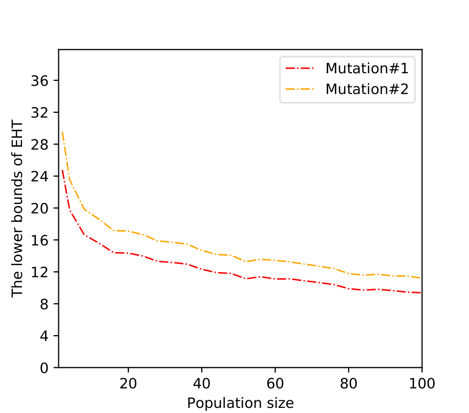
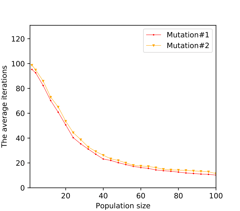
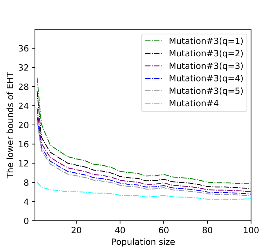
Figure 2: The theoretical and experimental running times of the ($\lambda$+$\lambda$)-ENAS algorithms using mutation operators Mutation#1, Mutation#2, Mutation#3 and Mutation#4, respectively, where population sizes $\lambda$ range from 1 to 100 with step size 4, and search space is set to $n=26$ and $L=2$. (a) The lower bounds of EHT of ($\lambda$+$\lambda$)-ENAS algorithms with one-bit mutation operators (Mutation#1 and Mutation#2). (b) The average iterations of the ($\lambda$+$\lambda$)-ENAS algorithms with Mutation#1 and Mutation#2. (c) The lower bounds of EHT of ($\lambda$+$\lambda$)-ENAS algorithms with $q$-bit mutation operator and bitwise mutation operator (Mutation#3 and Mutation#4). (d) The average iterations of the ($\lambda$+$\lambda$)-ENAS algorithms with Mutation#3 ($q=1,2,3,4,5$) and Mutation#4.

The theoretical and experimental results of the running time of the ($\lambda$+$\lambda$)-ENAS algorithms using different mutation operators have shown in Fig. 2, where Fig. 2 and Fig. 2 portray the theoretical running time, i.e., the lower bounds of EHT, and Fig. 2 and Fig. 2 depict the experimental running time, i.e., the average generations. The theoretical results Fig. 2 and Fig. 2 illustrate that the lower bound of EHT decreases as the population size increases; meanwhile, experimental results Fig. 2 and Fig. 2 demonstrate that the generation number of algorithm decreases strictly as the population increases. This finding illustrates that our theory can effectively capture the function of the population in the ENAS algorithm, i.e., the number of generations can be appropriately reduced when increasing the population size.

By comparing theoretical and experimental results, i.e., comparing Fig. 2 with Fig. 2 and comparing Fig. 2 with Fig. 2, we can find that the theoretical and experimental trends in the running time of different mutation operators in relation to the population size are approximately the same, and both point to the superiority of Mutation#1 operator over Mutation#2 operator and Mutation#4 operator over Mutation#3 operator. From the comparison, we can further find that when the population size is larger than 50, the theoretical and experimental results of using one-bit operators are extremely close and ranges from 10 to 20. This finding can provide theoretical insight for setting the generations of peer ENAS algorithm runs around 20 rather than other less reliable values.

Overall, the above findings on the relationship between specific NAS problem (NAS-Bench-101 searching problem) and algorithm parameters (generations, populations, and mutation operators) demonstrate that our theoretical analysis framework can successfully depict the algorithm runtime trend, which is of great significance for configuring an efficient and reliable ENAS algorithm. By conducting a similar theoretical approach, we can further analyze other NAS problems and gain some insights for designing new ENAS algorithms.

VI Conclusion

The paper aims to theoretically investigate the expected running time of the ($\lambda$+$\lambda$)-ENAS algorithm with various operators, so that the algorithm parameters and operators effectively supporting its running can be appropriately scheduled in advance. The theoretical investigation has been achieved by estimating the lower bound of the EHT through the proposed CEHT-ENAS framework. Specifically, in the proposed CEHT-ENAS, we present the common configuration to encode the complex structure of deep architectures and then introduce the partition method to measure the progress. Following, we give five lemmas to estimate the transition probabilities of different mutation operators under binary encoding and combination encoding mechanisms. By exploiting the CEHT-ENAS framework, the lower bounds of EHT regarding ($\lambda$+$\lambda$)-ENAS using different mutation operators are derived. Particularly, two theorems are given from the perspective of one-bit mutation, i.e., Theorems 1 and 2, and two theorems are given from the perspective of multi-bit mutation (including bitwise mutation), i.e., Theorems 3 and 4. Based on the proposed theorems, one case in terms of a particular NAS problem is studied to demonstrate the effectiveness of the proposed framework. We obtain the theoretical results through the case study and compare them with experimental results. The results show that, on the NAS-Bench-101 architecture searching problem, the “bit-based fair mutation” strategy outperforms the “offspring-based fair mutation” strategy in the ($\lambda$+$\lambda$)-ENAS algorithms using one-bit mutation operators. For ($\lambda$+$\lambda$)ENAS algorithms using multipoint mutation operators, the bitwise mutation operator usually outperforms the $q$-bit mutation operator. As a consequence, we are able to gain insight toward the relationship between some algorithmic features and problem characteristics, and thus, move closer toward the ultimate goal of guiding the design of new ENAS algorithms in practice using theoretical insight. To the best of our knowledge, this is the first work focusing on the theoretical analysis of ENAS algorithms. However, further studies are needed in analyzing the ENAS algorithm on more complex problems. The study presented in this paper serves as a solid and necessary foundation for such future work.

References

- [1] K. Simonyan and A. Zisserman, “Very deep convolutional networks for large-scale image recognition,” arXiv preprint arXiv:1409.1556, 2014.
- [2] K. He, X. Zhang, S. Ren, and J. Sun, “Deep residual learning for image recognition,” in Proceedings of the IEEE Conference on Computer Vision and Pattern Recognition, 2016, pp. 770–778.
- [3] H. Jie, S. Li, and S. Gang, “Squeeze-and-excitation networks,” in 2018 IEEE/CVF Conference on Computer Vision and Pattern Recognition, 2018.
- [4] A. Howard, M. Sandler, G. Chu, L.-C. Chen, B. Chen, M. Tan, W. Wang, Y. Zhu, R. Pang, V. Vasudevan et al., “Searching for mobilenetv3,” in Proceedings of the IEEE/CVF International Conference on Computer Vision, 2019, pp. 1314–1324.
- [5] K. Han, Y. Wang, Q. Tian, J. Guo, and C. Xu, “Ghostnet: More features from cheap operations,” in 2020 IEEE/CVF Conference on Computer Vision and Pattern Recognition, 2020.
- [6] Z. Li, F. Liu, W. Yang, S. Peng, and J. Zhou, “A survey of convolutional neural networks: analysis, applications, and prospects,” IEEE Transactions on Neural Networks and Learning Systems, 2021.
- [7] G. Huang, Z. Liu, L. Van Der Maaten, and K. Q. Weinberger, “Densely connected convolutional networks,” in Proceedings of the IEEE Conference on Computer Vision and Pattern Recognition, 2017, pp. 4700–4708.
- [8] J. Devlin, M.-W. Chang, K. Lee, and K. Toutanova, “Bert: Pre-training of deep bidirectional transformers for language understanding,” arXiv preprint arXiv:1810.04805, 2018.
- [9] Y. Zhang, W. Chan, and N. Jaitly, “Very deep convolutional networks for end-to-end speech recognition,” in 2017 IEEE International Conference on Acoustics, Speech and Signal Processing. IEEE, 2017, pp. 4845–4849.
- [10] T. Elsken, J. H. Metzen, and F. Hutter, “Neural architecture search: A survey,” The Journal of Machine Learning Research, vol. 20, no. 1, pp. 1997–2017, 2019.
- [11] B. Zoph and Q. V. Le, “Neural architecture search with reinforcement learning,” arXiv preprint arXiv:1611.01578, 2016.
- [12] C. Liu, B. Zoph, M. Neumann, J. Shlens, W. Hua, L.-J. Li, L. Fei-Fei, A. Yuille, J. Huang, and K. Murphy, “Progressive neural architecture search,” in Proceedings of the European Conference on Computer Vision, 2018, pp. 19–34.
- [13] H. Liu, K. Simonyan, and Y. Yang, “DARTS: Differentiable architecture search,” arXiv preprint arXiv:1806.09055, 2018.
- [14] Y. Xu, L. Xie, X. Zhang, X. Chen, G.-J. Qi, Q. Tian, and H. Xiong, “PC-DARTS: Partial channel connections for memory-efficient architecture search,” arXiv preprint arXiv:1907.05737, 2019.
- [15] X. Chu, T. Zhou, B. Zhang, and J. Li, “Fair DARTS: Eliminating unfair advantages in differentiable architecture search,” in European Conference on Computer Vision. Springer, 2020, pp. 465–480.
- [16] Y. Liu, Y. Sun, B. Xue, M. Zhang, G. G. Yen, and K. C. Tan, “A survey on evolutionary neural architecture search,” IEEE Transactions on Neural Networks and Learning Systems, 2021.
- [17] X. Yao, “Evolving artificial neural networks,” Proceedings of the IEEE, vol. 87, no. 9, pp. 1423–1447, 1999.
- [18] K. O. Stanley and R. Miikkulainen, “Evolving neural networks through augmenting topologies,” Evolutionary Computation, vol. 10, no. 2, pp. 99–127, 2002.
- [19] K. O. Stanley, D. B. D’Ambrosio, and J. Gauci, “A hypercube-based encoding for evolving large-scale neural networks,” Artificial Life, vol. 15, no. 2, pp. 185–212, 2009.
- [20] S. Risi, J. Lehman, and K. O. Stanley, “Evolving the placement and density of neurons in the hyperneat substrate,” in Proceedings of the 12th Annual Conference on Genetic and Evolutionary Computation, 2010, pp. 563–570.
- [21] E. Real, S. Moore, A. Selle, S. Saxena, Y. L. Suematsu, J. Tan, Q. V. Le, and A. Kurakin, “Large-scale evolution of image classifiers,” in International Conference on Machine Learning, 2017, pp. 2902–2911.
- [22] Y. Sun, B. Xue, M. Zhang, and G. G. Yen, “Completely automated CNN architecture design based on blocks,” IEEE Transactions on Neural Networks and Learning Systems, vol. 31, no. 4, pp. 1242–1254, 2019.
- [23] E. Real, A. Aggarwal, Y. Huang, and Q. V. Le, “Regularized evolution for image classifier architecture search,” in Proceedings of the AAAI Conference on Artificial Intelligence, vol. 33, no. 01, 2019, pp. 4780–4789.
- [24] K. O. Stanley, J. Clune, J. Lehman, and R. Miikkulainen, “Designing neural networks through neuroevolution,” Nature Machine Intelligence, vol. 1, no. 1, pp. 24–35, 2019.
- [25] Y. Xue, Y. Wang, J. Liang, and A. Slowik, “A self-adaptive mutation neural architecture search algorithm based on blocks,” IEEE Computational Intelligence Magazine, vol. 16, no. 3, pp. 67–78, 2021.
- [26] T. Jansen, I. Wegener, and P. Kaufmann, “On the utility of populations in evolutionary algorithms,” in Proceedings of the Genetic and Evolutionary Computation Conference, 2001, pp. 1034–1041.
- [27] C. Witt, “Runtime analysis of the (+1) EA on simple pseudo-Boolean functions,” Evolutionary Computation, vol. 14, no. 1, pp. 65–86, 2006.
- [28] T. Storch, “On the choice of the parent population size,” Evolutionary Computation, vol. 16, no. 4, pp. 557–578, 2008.
- [29] C. Witt, “Population size versus runtime of a simple evolutionary algorithm,” Theoretical Computer Science, vol. 403, no. 1, pp. 104–120, 2008.
- [30] B. Doerr and M. Künnemann, “Optimizing linear functions with the (1+ ) evolutionary algorithm—different asymptotic runtimes for different instances,” Theoretical Computer Science, vol. 561, pp. 3–23, 2015.
- [31] C. Gießen and C. Witt, “Population size vs. mutation strength for the (1+ ) EA on OneMax,” in Proceedings of the 2015 Annual Conference on Genetic and Evolutionary Computation, 2015, pp. 1439–1446.
- [32] T. Chen, J. He, G. Sun, G. Chen, and X. Yao, “A new approach for analyzing average time complexity of population-based evolutionary algorithms on unimodal problems,” IEEE Transactions on Systems, Man, and Cybernetics, Part B (Cybernetics), vol. 39, no. 5, pp. 1092–1106, 2009.
- [33] P. K. Lehre and X. Yao, “On the impact of mutation-selection balance on the runtime of evolutionary algorithms,” IEEE Transactions on Evolutionary Computation, vol. 16, no. 2, pp. 225–241, 2011.
- [34] T. Chen, K. Tang, G. Chen, and X. Yao, “A large population size can be unhelpful in evolutionary algorithms,” Theoretical Computer Science, vol. 436, pp. 54–70, 2012.
- [35] C. Qian, Y. Yu, and Z.-H. Zhou, “A lower bound analysis of population-based evolutionary algorithms for pseudo-Boolean functions,” in International Conference on Intelligent Data Engineering and Automated Learning. Springer, 2016, pp. 457–467.
- [36] D. Antipov and B. Doerr, “A tight runtime analysis for the (+) EA,” Algorithmica, vol. 83, no. 4, pp. 1054–1095, 2021.
- [37] G. Rudolph, “Convergence properties of evolutionary algorithms.” in Verlag Dr Kovac, 1997.
- [38] H. Mühlenbein and D. Schlierkamp-Voosen, “Predictive models for the breeder genetic algorithm i. continuous parameter optimization,” Evolutionary Computation, vol. 1, no. 1, pp. 25–49, 1993.
- [39] J. He and X. Yao, “Average drift analysis and population scalability,” IEEE Transactions on Evolutionary Computation, vol. 21, no. 3, pp. 426–439, 2016.
- [40] Z.-H. Zhou, Y. Yu, and C. Qian, Evolutionary Learning: Advances in Theories and Algorithms. Springer, 2019.
- [41] B. Doerr and F. Neumann, Theory of evolutionary computation: Recent developments in discrete optimization. Springer Nature, 2020.
- [42] I. Wegener, Methods for the Analysis of Evolutionary Algorithms on Pseudo-Boolean Functions. Springer US, 2002, pp. 349–369. [Online]. Available: https://doi.org/10.1007/0-306-48041-7_14
- [43] P. K. Lehre, “Fitness-levels for non-elitist populations,” in Proceedings of the 13th Annual Genetic and Evolutionary Computation Conference, 2011, pp. 2075–2082.
- [44] J. Lässig and D. Sudholt, “General upper bounds on the runtime of parallel evolutionary algorithms,” Evolutionary Computation, vol. 22, no. 3, pp. 405–437, 2014.
- [45] D. Corus, D.-C. Dang, A. V. Eremeev, and P. K. Lehre, “Level-based analysis of genetic algorithms and other search processes,” IEEE Transactions on Evolutionary Computation, vol. 22, no. 5, pp. 707–719, 2017.
- [46] Y. Yu and Z.-H. Zhou, “A new approach to estimating the expected first hitting time of evolutionary algorithms,” Artificial Intelligence, vol. 172, no. 15, pp. 1809–1832, 2008.
- [47] J. He and X. Yao, “Drift analysis and average time complexity of evolutionary algorithms,” Artificial Intelligence, vol. 127, no. 1, pp. 57–85, 2001.
- [48] ——, “A study of drift analysis for estimating computation time of evolutionary algorithms,” Natural Computing, vol. 3, no. 1, pp. 21–35, 2004.
- [49] P. S. Oliveto and C. Witt, “Simplified drift analysis for proving lower bounds in evolutionary computation,” Algorithmica, vol. 59, no. 3, pp. 369–386, 2011.
- [50] J. Lengler, “Drift analysis,” in Theory of Evolutionary Computation. Springer Nature, 2020, pp. 89–131.
- [51] P. K. Lehre and P. S. Oliveto, “Runtime analysis of population-based evolutionary algorithms: introductory tutorial at GECCO 2020,” in Proceedings of the 2020 Genetic and Evolutionary Computation Conference Companion, 2020, pp. 458–494.
- [52] C. Ying, A. Klein, E. Christiansen, E. Real, K. Murphy, and F. Hutter, “Nas-bench-101: Towards reproducible neural architecture search,” in International Conference on Machine Learning, 2019, pp. 7105–7114.
- [53] Á. E. Eiben, R. Hinterding, and Z. Michalewicz, “Parameter control in evolutionary algorithms,” IEEE Transactions on Evolutionary Computation, vol. 3, no. 2, pp. 124–141, 1999.
- [54] J. He and X. Yao, “Towards an analytic framework for analysing the computation time of evolutionary algorithms,” Artificial Intelligence, vol. 145, no. 1-2, pp. 59–97, 2003.
- [55] ——, “From an individual to a population: An analysis of the first hitting time of population-based evolutionary algorithms,” IEEE Transactions on Evolutionary Computation, vol. 6, no. 5, pp. 495–511, 2002.
- [56] J. Jägersküpper, “A blend of Markov-chain and drift analysis,” in International Conference on Parallel Problem Solving from Nature. Springer, 2008, pp. 41–51.
- [57] J. He, T. Chen, and X. Yao, “On the easiest and hardest fitness functions,” IEEE Transactions on evolutionary computation, vol. 19, no. 2, pp. 295–305, 2014.
- [58] C. Witt, “On crossing fitness valleys with majority-vote crossover and estimation-of-distribution algorithms,” in Proceedings of the 16th ACM/SIGEVO Conference on Foundations of Genetic Algorithms, 2021, pp. 1–15.
- [59] G. Rudolph, “Convergence analysis of canonical genetic algorithms,” IEEE Transactions on Neural Networks, vol. 5, no. 1, pp. 96–101, 1994.