Sequential Ensembling for Semantic Segmentation

Abstract

Ensemble approaches for deep-learning-based semantic segmentation remain insufficiently explored despite the proliferation of competitive benchmarks and downstream applications. In this work, we explore and benchmark the popular ensembling approach of combining predictions of multiple, independently-trained, state-of-the-art models at test time on popular datasets. Furthermore, we propose a novel method inspired by boosting to sequentially ensemble networks that significantly outperforms the naïve ensemble baseline. Our approach trains a cascade of models conditioned on class probabilities predicted by the previous model as an additional input. A key benefit of this approach is that it allows for dynamic computation offloading, which is useful for deploying models on mobile devices. Our proposed novel ADaptive modulatiON (ADON) block allows spatial feature modulation at various layers using previous stage probabilities. Our approach does not require any sophisticated sample selection strategies during training, and works with multiple neural architectures. We significantly improve over the naïve ensemble baseline on challenging datasets such as Cityscapes, ADE-20K, COCO-Stuff and PASCAL-Context and set a new state-of-the-art.

1 Introduction

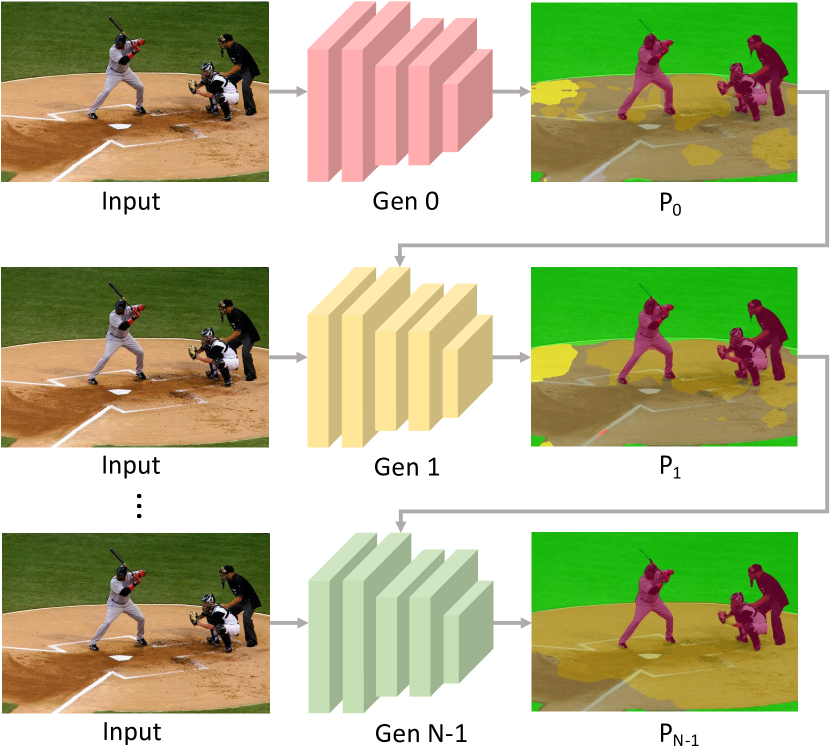
Figure 1: Sequential Ensembling: We sequentially train $N$ generations as a cascade. Each generation predicts segmentation probabilities from the input image conditioned on the segmentation probabilities from the previous generation.

Semantic segmentation, i.e., pixel classification, is a fundamental task in computer vision with applications in a wide variety of domains, such as autonomous driving [56], robotic navigation [43], medical analysis [50], and scene understanding [81]. Over the years, deep learning based semantic segmentation methods have achieved remarkable performance  [73, 42, 72, 1, 45, 74, 70]. Most of these approaches focus on training a single network with novel architectures and loss functions to improve performance, overlooking the extensive classical literature on ensembles [2, 54, 62]. Ensembles have been shown to improve accuracy [3], uncertainty estimation, and out-of-distribution robustness [16]. We argue that deep learning approaches can benefit greatly from the pioneering work done in ensemble learning. In this paper, we methodically explore deep ensembles for semantic segmentation with the goal of further improving performance of state-of-the-art semantic segmentation models.

A naïve deep ensembling approach is to train multiple networks and fuse their outputs (e.g., average their predicted probabilities). We benchmark this ensembling approach for state-of-the-art deep semantic segmentation models across multiple datasets. Similar to [37, 5, 65], the baseline ensembling rule averages predicted probabilities using equal weight for all the models within the ensemble. We refer to this as simple ensembling (SIM-ENS). Consistent with [5, 65], and as shown in Tab. 1, we observe diminishing returns as the number of models $N$ in the ensemble increases. For dense per-pixel predictions, simple ensembles are not effective as distinct models perform well on different regions of the image. A natural variation is to try other ensembling rules such as max-voting and weighted-averaging using model confidence estimates [10]. However, these strategies result in moderate gains similar to simple ensembles as shown in Tab. 1, owing to challenges in obtaining reliable per pixel confidence weights (see Fig. 3).

In this work, we propose sequential ensembling as an alternative to simple ensembling. Sequential ensembling (SEQ-ENS) is a data-driven approach to learn an optimal ensemble compared to ad-hoc ensembling approaches (e.g., averaging or voting). Inspired by boosting [53] and cascaded refinement [47, 8], we train $N$ generations of deep models sequentially, as shown in Fig. 1. Generation $G_{i}$ uses input image $\mathbf{I}$ and the predicted probability map $\mathbf{P}_{i-1}$ from generation $G_{i-1}$ to predict $\mathbf{P}_{i}$. Our approach only requires probability maps from the previous generation and does not require any sophisticated sample selection strategy during training. To condition on probability maps, we adopt the simple yet effective mechanism of feature modulation [49, 13, 25]. We propose a novel ADaptive modulatiON (ADON) block which injects information from $\mathbf{P}_{i-1}$ at multiple depths within the network. Dense prediction is aided by spatial context and the ADON block allows spatial modulation of intermediate features of $G_{i}$. Each subsequent generation learns to incorporate knowledge from the previous generation using class-specific spatial context. Unlike simple ensembles, each model can dedicate network capacity to correct mistakes made by prior generations. Our approach allows for increase in accuracy as the ensemble size is increased, as shown for multiple datasets in Fig. 2.

Method	Cityscapes	ADE20K	COCO-Stuff
Single Model ($N=1$)	76.2	33.1	32.4
SIM-ENS ($N=2$)	77.1 (+0.9)	34.5 (+1.4)	33.5 (+1.1)
SIM-ENS ($N=5$)	77.5 (+1.3)	34.9 (+1.8)	33.8 (+1.4)
SIM-ENS ($N=15$)	77.8 (+1.6)	35.8 (+2.7)	34.9 (+2.5)
Voting Ens. ($N=15$)	76.9 (+0.7)	35.3 (+2.2)	35.1 (+2.7)
W-Avg. Ens. ($N=15$)	78.0 (+1.8)	35.0 (+1.9)	34.6 (+2.2)
SEQ-ENS ($N=2$)	78.9 (+2.7)	37.6 (+4.5)	36.3 (+3.9)

Table 1: Sequential ensembling (SEQ-ENS) offers significantly higher improvement (mIOU) compared to traditional ensembling approaches based on voting and simple/weighted averaging. Results are reported on the val sets using HRNetW18s-v2 [58] backbone with single-scale testing.

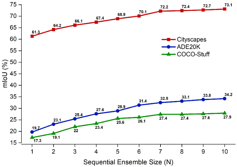
Figure 2: Performance of Sequential Ensembling using FCN [45] MobileNetv2-D8 [52] backbone on the val set of various datasets using single-scale testing. We see increase in performance as more stages are added, allowing run-time trade-off between accuracy and speed for edge devices.

Sequential ensembles are constructed by training a new generation with parameters of all previous generations $\{G_{i-1},G_{i-2},\dots G_{0}\}$ frozen. This affords several important benefits. For example, the sequential chain can be interrupted at any depth, and each stage can still output pixel-wise probabilities. This is a valuable property that allows for dynamic computation offloading [46] where the ensemble size can be adjusted on the fly to meet resource limitations without any retraining. This strategy is useful for deploying models on diverse mobile platforms to best suit changing on-device constraints, e.g., diminishing battery life, applications that require accuracy vs. runtime tradeoffs (fast previews vs. slow high-quality results), responsiveness requirements in the context of changing mission-critical workloads.

Our proposed approach achieves state-of-the-art results on Cityscapes [9], ADE20K [80], PASCAL-Context [48] and COCO-Stuff [4]. For backbones with lower computational complexity, sequential ensembles $(N=2)$ outperforms simple ensembles $(N=15)$ across multiple datasets, as shown in Tab. 1. In Tab. 5, we additionally show that a $2$ model sequential ensemble with single-scale inference outperforms a single model with multi-scale test-time augmentation using $12$ inferences ($6$x lower inferences). Furthermore, we show that sequential models can (a) generalize across different backbone architectures (Tab. 2), (b) exhibit self-improvement via the ability to refine their own segmentation maps iteratively yielding non-trivial gains (Tab. 7) and (c) can be used to create general neural network graphs leveraging diversity gains from ensembling (Tab. 8).

In summary:

• We explore ensembling approaches for deep neural networks to improve state-of-the-art segmentation networks and provide an ensembling benchmark of various models across multiple semantic segmentation datasets.

• Our proposed sequential ensembling outperforms naïve ensembling methods and advances the state-of-the-art on challenging benchmarks.

• Our proposed feature modulation ADON blocks efficiently incorporates information from previous generations in the sequential ensemble chains.

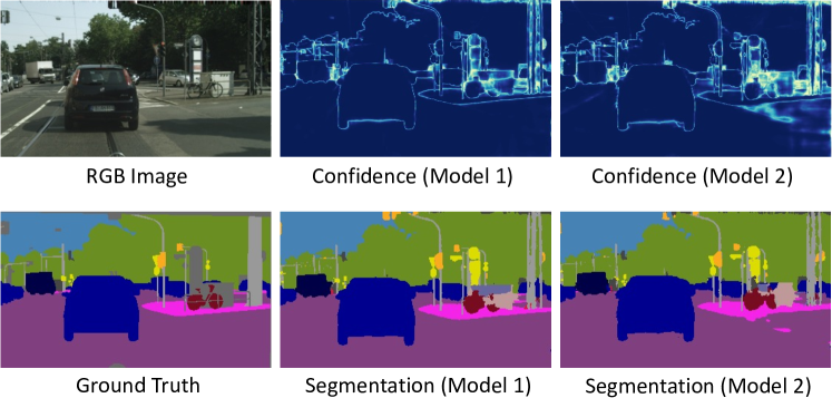
Figure 3: Heatmap visualization of per-pixel confidence (max class probability) of independently trained models (blue is high confidence). We observe that confidence on a pixel is not necessarily correlated with accuracy of segmentation model. Empirically, our method performs better than confidence weighted ensembling rule.

2 Related Work

Semantic-Segmentation: Semantic segmentation is an extension of the classification problem from image level to pixel level. Over the past few years, advances in deep learning for image classification [21, 37, 57, 12, 64, 61, 55] led to significant improvements for semantic segmentation [58, 45, 44, 50, 74]. These efforts benefited from the introduction of popular datasets such as Cityscapes [9], ADE20K [80], PASCAL-Context [48], PASCAL-VOC [15], COCO-Stuff [4], etc. In this work, we benchmark ensembling for segmentation.

Ensembles for Segmentation: Ensemble learning has been well-studied in machine learning; seminal works include bagging [2], boosting [53], and AdaBoost [17]. Ensembles of deep models have been used to boost performance on many tasks such as image classification [59, 24], machine translation [66] and uncertainty estimation [39, 16, 67, 78]. However, ensembling approaches have not been fully explored for semantic segmentation owing to computational challenges in dense pixel prediction. Our work benchmarks ensembles of state-of-the-art models across various segmentation datasets [9, 80, 48, 34, 4, 15] and model families [58, 45, 71]. We hope this will be helpful in inspiring and evaluating new ideas in field. Further, inspired by boosting paradigm [53], our proposed sequential ensemble methodology achieves new state-of-the-art segmentation results.

Segmentation Refinement: Many refinement methods [20, 11, 38, 42, 28, 40, 75, 29] have been proposed. These refinement approaches depend on the segmentation model [40], super-pixels [11], multi-scale input [42], data-generation [32], or object boundary information [75]. In contrast to [75] which assumes that most errors are at object boundaries, our approach does not make any such assumptions and can be applied to improve segmentation predictions at pixels away from boundaries, especially for lighter models (e.g. MobileNets [52]). Sequential ensembles offer a principled way of conditioning on probability outputs from a given model. The sequential nature allows training more than one refinement models and offers trade-off between accuracy/speed at run-time.

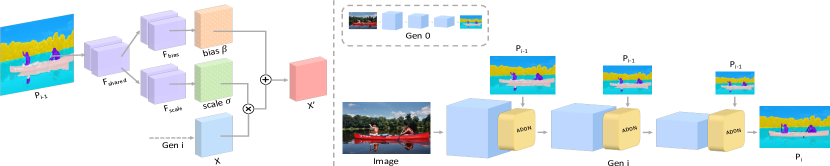
Figure 4: Left: ADaptive ModulatiON (ADON) Block (in gold) learns parameters scale $\bm{\sigma}$ and bias $\bm{\beta}$ for spatial affine transformation of intermediate features $\mathbf{X}$ (in blue) from the segmentation probability map $\mathbf{P}_{i-1}$. Right: Introduction of ADON blocks at various depths allows conditioning on spatial probability maps at various levels within the network.

Feature Modulation Methods: Various forms of feature modulation methods have proven highly effective across a number of domains: Conditional Instance Norm [13, 19], Adaptive Instance Norm [25] for neural style transfer, Dynamic Layer Norm [35] for speech recognition, FiLM [49] for visual question answering, and MIMB [31, 33] for pose estimation. We show that feature-wise affine conditioning is effective in conditioning models in a cascade for high-resolution semantic segmentation.

3 Method

Semantic segmentation aims to classify pixels in an input image $\mathbf{I}\in\mathbb{R}^{H\times W\times 3}$ into $C$ classes. Most methods, e.g., [58, 6, 77], transform this problem to estimating per-pixel class probabilities to create a probability map $\mathbf{P}\in\mathbb{R}^{H\times W\times C}$ from $\mathbf{I}$ using a deep network $G$ such that $\mathbf{P}=G(\mathbf{I})$. The segmentation network $G$ is trained in a supervised way to minimize loss $\mathcal{L}(\mathbf{Y},\mathbf{P})$ [30], where $\mathbf{Y}$ is the ground truth segmentation map of image $\mathbf{I}$. At inference, each pixel is assigned the label corresponding to the highest probability.

Simple Ensembles: Consider a pretrained model ensemble $\mathcal{B}$ with $N$ segmentation models, $\mathcal{B}=\{B_{0},B_{1},\dots,B_{N-1}\}$, where each ensemble member $B_{i}$ is independently trained. The prediction $\mathbf{P}$ of the ensemble $\mathcal{B}$ on the input image $\mathbf{I}$ can be defined as follows:

$$\mathbf{P}_{i} = B_{i}(\mathbf{I}).$$ (1)

$$\mathbf{P} = \mathcal{B}(\mathbf{I}),$$ (2)

$$= \Phi\big{(}\mathbf{P}_{0},\mathbf{P}_{1},\dots,\mathbf{P}_{N-1}\big{)},$$ (3)

where $\Phi$ is a strategy to combine individual model predictions, e.g.,

$$\Phi = \frac{1}{N}\sum_{i=0}^{N-1}\mathbf{w}_{i}\mathbf{P}_{i},$$ (4)

where $\mathbf{w}_{i}$ can be uniform (average) or vary as a function of output probabilities (weighted average). Other strategies such as median averaging, majority voting, stacking [68], or selecting best model [14] can also be used to define $\Phi$. Designing an optimal $\Phi$ for semantic segmentation is crucial, yet challenging since different models in an ensemble may be more accurate on different regions of an image.

3.1 Sequential Ensembles

We propose a sequential ensembling strategy that avoids the combination rule $\Phi$ and learns an optimal ensembling from the training data. Let $\mathcal{G}=\{G_{0},G_{1},\dots,G_{N-1}\}$ be $N$ segmentation models in the sequential ensemble. Each model $G_{i}$ forms a Markov chain of conditional dependence on the previous models $G_{i-1},\dots G_{0}$ as follows.

$$\mathbf{P}_{0} = G_{0}(\mathbf{I}),$$ (5)

$$\mathbf{P}_{i} = G_{i}(\mathbf{I},\mathbf{P}_{i-1}).$$ (6)

Each model in the sequential ensemble is trained to predict $\mathbf{P}$ given the input image, conditioned on the previous model’s prediction as shown in Fig. 1. This allows each new model in the ensemble the opportunity to correct errors made by the previous model in the chain.

Method	Arch	Cityscapes (val)												ADE-20K	COCO-Stuff	PASCAL-Cnxt
		wall	fnce	tlgt	tsgn	prsn	ridr	trck	bus	train	mcyl	bcyl	mIoU
Class (%) $\rightarrow$		0.6	0.7	0.2	0.6	1.1	0.2	0.3	0.3	0.1	0.1	0.6		(val)	(test)	(test)
MobileNetv3 [22]	D8s	39.4	47.0	45.1	63.1	71.1	45.1	45.7	64.7	51.5	39.3	67.0	64.1	29.7	24.1	32.7
SIM-ENS	D8s	41.1	49.1	48.1	65.4	73.4	46.4	47.9	68.2	51.5	44.1	68.3	65.4 (+1.3)	31.4 (+1.7)	26.3 (+2.2)	34.2 (+1.5)
SEQ-ENS (Ours)	D8s	42.6	52.4	52.7	68.3	74.5	48.8	54.6	70.8	51.8	47.9	69.5	68.7 (+4.6)	35.3 (+5.6)	28.6 (+4.5)	36.9 (+4.2)
MobileNetv3 [22]	D8	48.3	51.4	57.7	69.6	75.5	50.1	58.4	73.5	51.6	50.3	70.6	69.5	31.8	26.8	34.4
SIM-ENS	D8	49.0	53.5	60.4	71.6	76.4	53.7	62.1	74.5	53.7	54.8	73.1	71.1 (+1.6)	33.9 (+2.1)	28.5 (+1.7)	36.0 (+1.6)
SEQ-ENS (Ours)	D8	50.3	56.8	65.0	78.9	78.1	57.8	68.9	75.1	57.4	59.4	75.4	73.6 (+4.1)	35.6 (+3.8)	30.0 (+3.2)	37.3 (+2.9)
HRNet [58]	H-18s	53.2	61.5	70.3	77.9	81.1	59.2	66.4	84	70.5	59.7	76.1	76.2	33.1	29.4	38.9
SIM-ENS	H-18s	56.3	61.1	71.8	79.4	82.4	61.6	69.4	84.4	67.5	61.9	77.0	77.1 (+0.9)	34.5 (+1.4)	30.0 (+0.6)	40.4 (+1.5)
SEQ-ENS (Ours)	H-18s	59	63.9	73.6	79.6	82.8	62.2	75.5	88	78	63.4	78.2	78.9 (+2.7)	37.6 (+4.5)	32.7 (+3.3)	42.0 (+3.1)
HRNet [58]	H-18	59.1	63.7	73.2	80.6	82.8	61.8	75.9	87.7	75.5	60.4	77.3	78.7	36.8	33.0	42.6
SIM-ENS	H-18	59.2	63.6	74.1	81.1	83.1	62.0	76.5	87.8	74.3	60.7	78.1	79.0 (+0.3)	37.6 (+0.8)	34.1 (+1.1)	43.9 (+1.3)
SEQ-ENS (Ours)	H-18	58.0	64.6	75.0	82.0	84.0	63.2	79.1	90.1	78.6	62.7	79.1	79.8(+1.1)	40.9 (+4.1)	35.7 (+2.7)	46.1 (+3.5)
HRNet [58]	H-48	56.4	65.6	75.5	81.9	84.1	66.3	79.7	89.8	84.2	68.8	80.1	80.5	42.0	38.3	51.1
SIM-ENS	H-48	56.6	65.1	75.8	82.1	84.2	67.1	79.8	89.9	84.6	68.3	79.9	80.6 (+0.1)	42.5 (+0.5)	39.7 (+1.4)	52.1 (+1.0)
SEQ-ENS (Ours)	H-48	58.9	66.9	76.8	83.2	84.8	68.3	80.1	90.6	85.6	68.8	80.9	81.3 (+0.8)	45.6 (+3.6)	40.8 (+2.5)	53.8 (+2.7)
DeepLabv3+ [7]	R-18	51.4	58.2	69.9	77.6	81.3	60.8	76.1	85.4	72.5	63.1	76.3	76.8	34.1	29.7	43.5
SIM-ENS	R-18	51.1	58.3	71.5	78.9	82.1	61.0	77.8	87.3	74.5	64.3	76.9	77.8 (+1.0)	35.4 (+1.3)	31.2 (+1.5)	45.8 (+2.3)
SEQ-ENS (Ours)	R-18	51.2	59.4	74.6	80.8	83.6	62.8	79.8	88.1	77.0	67.2	78.3	78.9 (+2.1)	37.6 (+3.5)	35.3 (+4.1)	46.2 (+2.7)
DeepLabv3+ [7]	R-50	51.2	62.5	74.3	82.2	84.2	65.8	81.1	88.8	84.7	68.6	79.5	79.8	42.7	37.4	50.4
SIM-ENS	R-50	51.8	62.8	74.5	82.8	84.6	65.9	81.4	89.8	85.1	69.2	79.8	80.1 (+0.3)	43.3 (+0.6)	38.2 (+0.8)	51.8 (+1.4)
SEQ-ENS (Ours)	R-50	53.4	63.2	75.6	83.5	85.0	66.3	79.3	91.9	85.2	70.0	80.2	80.7 (+0.9)	45.1 (+2.4)	39.2 (+1.8)	52.4 (+2.0)
DeepLabv3+ [7]	R-101	54.9	64.4	74.6	81.9	84.6	67.7	85.2	91.8	85.2	71.3	80.3	80.9	44.6	38.8	53.2
SIM-ENS	R-101	55.1	64.6	74.7	82.0	84.7	67.8	85.0	91.9	85.8	71.9	80.3	81.1 (+0.2)	45.0 (+0.4)	39.0 (+0.2)	54.0 (+0.8)
SEQ-ENS (Ours)	R-101	56.0	64.6	75.2	82.6	84.9	68.5	85.4	92.3	86.5	72.5	80.5	81.5 (+0.6)	46.8 (+2.2)	40.3 (+1.3)	55.1 (+1.9)

Table 2: Comparison of SEQ-ENS (Ours) with SIM-ENS using $N=2$ on various datasets. R-@ and H-@ stand for ResNet-@ and HRNet-W@ respectively. D8 is the output stride of DeepLabv3+. s denotes the small version of the backbone. We report class-wise mIoU for 11 rare classes in Cityscapes. For rare classes such as motor-cycle (mcycl), SEQ-ENS improves mIOU by $\approx 2X$ compared to SIM-ENS.

3.2 Adaptive Modulation Block

A key challenge is designing the architecture in order to take the previous generation’s probabilities as a conditioning input. A naïve early fusion approach would be to simply concatenate the input image $\mathbf{I}$ with the probability map $\mathbf{P}_{i-1}$ corresponding to the output of the previous generation. Similarly, late fusion would concatenate feature maps from later layers within the network with appropriately down-sampled probability map $\mathbf{P}_{i-1}$. However, both of these approaches fail to improve performance.

We describe the ADaptive modulatiON (ADON) block that can be easily introduced in any existing feature extraction backbone to overcome this issue (see Fig. 4). ADON allows spatial modulation of intermediate feature maps using the conditioning input $\mathbf{P}_{i-1}$. The $i^{\text{th}}$ generation model $G_{i}$ in the sequential ensemble uses ADON blocks to leverage information from the prediction $\mathbf{P}_{i-1}$ of the previous generation model. Similar to the Batch Normalization [27], ADON learns to adaptively influence the output of the neural network by applying an affine transformation to the network’s intermediate features based on $\mathbf{P}_{i-1}$.

Let $\mathbf{X}\in\mathbb{R}^{H^{\prime}\times W^{\prime}\times D}$ be an intermediate feature map in the segmentation network $G_{i}$. The ADON block consists of operations $\mathbf{F}_{\text{shared}}$, $\mathbf{F}_{\text{scale}}$ and $\mathbf{F}_{\text{bias}}$ on the probability map $\mathbf{P}_{i-1}$ from the previous generation $G_{i-1}$. The modulation outputs $\bm{\sigma}$ and $\bm{\beta}$ are used to element-wise scale and bias the intermediate feature map $\mathbf{X}$ to produce $\mathbf{X}^{\prime}$. We implement the operations $\mathbf{F}_{\text{shared}}$, $\mathbf{F}_{\text{scale}}$ and $\mathbf{F}_{\text{bias}}$ using a simple two-layer convolutional network, whose design is in the supplemental material. First, the probability map $\mathbf{P}_{i-1}\in\mathbb{R}^{H\times W\times C}$ is spatially downsampled to match the 2D resolution of $\mathbf{X}$. The operation $\mathbf{F}_{\text{shared}}$ then maps $\mathbf{P}_{i-1}\in\mathbb{R}^{H^{\prime}\times W^{\prime}\times D}$ to a $K$-dimensional latent space, $\mathbf{e}\in\mathbb{R}^{H^{\prime}\times W^{\prime}\times K}$. We use this latent space to predict the scale and bias parameters jointly using $\mathbf{F}_{\text{scale}}$ and $\mathbf{F}_{\text{bias}}$ where $\bm{\sigma},\bm{\beta}\in\mathbb{R}^{H^{\prime}\times W^{\prime}\times D}$.

$$\mathbf{e} = \mathbf{F}_{\text{shared}}(\mathbf{P}_{i-1}),$$ (7)

$$\bm{\sigma} = \mathbf{F}_{\text{scale}}(\mathbf{e}),$$ (8)

$$\bm{\beta} = \mathbf{F}_{\text{bias}}(\mathbf{e}),$$ (9)

$$\mathbf{X}^{\prime} = \bm{\sigma}*\mathbf{X}+\bm{\beta}.$$ (10)

Thus, ADON is a spatial generalization of channel-wise feature modulation blocks proposed in [23, 31]. As the modulation parameters are adaptive to the spatially variant input probability maps, the proposed ADON block is an effective way of injecting segmentation information at multiple layers within the network in comparison to early/late fusion [18]. ADON blocks inserted early in the network capture finer details such as object boundaries and those inserted late resolve the class confusion between similar looking classes.

4 Experiments

We evaluate our approach on the following datasets.

Cityscapes [9] is a real world driving dataset that consists of 2975 train, 500 val and 1525 test images with resolution $2048\times 1024$. The dataset contains $19$ semantic categories for the segmentation task.

ADE20K [80] is used in ImageNet scene parsing challenge 2016 consisting of around 20k train, 2k val, 3k test images spanning 150 fine-grained semantic categories and diverse scenes.

COCO-Stuff [4] is a challenging scene parsing dataset that contains 171 semantic classes. We use the smaller version with 10k images. The train set and test set consists of 9k and 1k images respectively.

PASCAL-Context [48] consists of 59 semantic classes and 1 background label. The dataset contains 4998 train and 5105 test images. We follow the standard testing procedure [58]. The image is resized to $480\times 480$ and then fed into our network. The resulting $480\times 480$ label maps are then resized to the original image size.

Implementation details. We use the mmsegmentation codebase for the implementation of various model families. We use the available pretrained models as $G_{0}$ in the sequential ensemble, and focus on improving their performance by adding additional generations. For fairness, the models in the later generations are trained with the same hyper-parameters as the $G_{0}$ model. We use the imagenet pretrained backbone for all our experiments. For SIM-ENS, the segmentation head of the backbone is randomly initialized across multiple runs. During training, we apply data augmentation using: random resize with ratio $0.5-2.0$, random horizontal flipping and random cropping for all datasets. The models are trained using either SGD [51] or AdamW [36] optimizer for 160k iterations. The learning rate is set to an initial value and then decayed using a polynomial LR schedule. We report semantic segmentation performance using mean Intersection over Union (mIoU) for all datasets. For the HRNet [58] family, we insert $10$ ADON blocks for Cityscapes and Pascal-Context datasets and $5$ ADON blocks for ADE20K and COCO-Stuff datasets. We use $K=128$ for all our experiments. Further, unless mentioned otherwise we report results using inference at single-scale and no flipping. Please refer to the supplemental for more details.

4.1 Comparisons with Simple Ensembles

We compare SEQ-ENS and SIM-ENS in Tab. 2 for $N=2$. We benchmark three model families, MobileNetv3 [22], HRNet [58], and DeepLabv3+ [7], with different backbones. SEQ-ENS consistently improves over SIM-ENS in all settings; relative improvements over baseline with respect to SIM-ENS range from $2$x to $8$x.

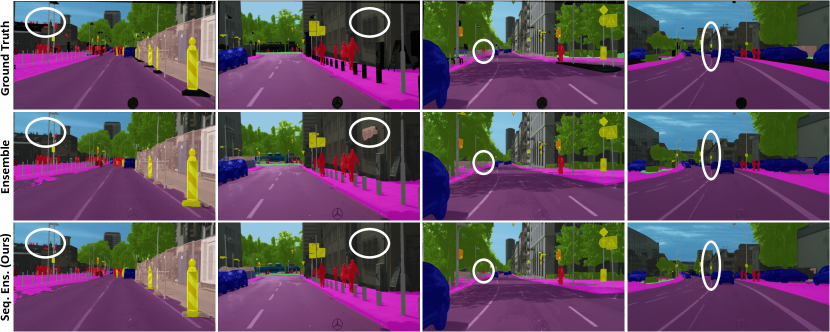
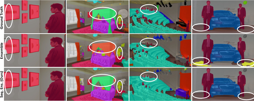
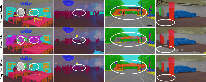
Figure 7: Qualitative comparison of Sequential Ensembles and Simple Ensembles. Cityscapes (first three rows) and ADE20K (last six rows) for HRNet-W48(N=2). The white eclipses highlight the fine-grained details that our approach captures in comparison to the baseline.

On Cityscapes, SEQ-ENS shows consistent gains across all backbones over SIM-ENS. Gains from SEQ-ENS tend to be more exaggerated for scenarios susceptible to underfitting compared to single models or SIM-ENS. For example, mIoU improves most significantly for rare categories, such as train and motorcycle, and categories with fine structures, such as pole and fence. This shows SEQ-ENS distributes model capacity intelligently to focus on underrepresented classes and finer details. Our improvements are especially pronounced when ensembling light models like MobileNetv3 or evaluating on complex datasets with more classes. For example, for H-18s, SEQ-ENS outperforms SIM-ENS by +1.6 mIOU for Cityscapes ($19$ categories) and +1.6 for PASCAL-Context ($59$ categories), but by +3.1 for ADE-20K ($150$ categories) and +2.7 for COCO-Stuff ($171$ categories). We show qualitative results in Fig. 7.

# Models	SIM-ENS		SEQ-ENS
	mIoU	Params	mIoU	Params	GFLOPs	FPS	Train-Epochs
N = 1	19.7	9.8	19.7	9.8	39.6	65	127
N = 2	20.6	19.6	23.1	20.4	80.6	36	201
N = 4	22.4	39.2	27.6	41.6	163.2	20	311
N = 6	23.3	58.8	31.4	62.8	245.6	15	387
N = 8	23.9	78.4	33.1	84.0	328.0	11	440
N = 10	24.8	98.1	34.2	105.2	410.4	9	495

Table 3: Metrics with varying $N$ for SIM-ENS and SEQ-ENS on ADE20K val set using FCN MobileNetv2-D8 [52].

Further, we report various metrics like mIoU, parameters (M), GFLOPs, test-time FPS and total training epochs with varying ensemble size (N) for SIM-ENS and SEQ-ENS in Tab. 3 using MobileNetv2 [52]. As can be seen, later generations require fewer epochs for training in SEQ-ENS due to quicker convergence (495 vs. 127 epochs for $10^{th}$ vs. $1^{st}$ generation). Finally, our method allows for a dynamic trade-off between accuracy and latency by varying the ensemble size during inference —a desirable property for edge devices.

4.2 Improving State-of-the-Art

We improve the state-of-the-art among methods that do not use extra data on the Cityscapes and ADE20K val sets. We construct a sequential ensemble of size $3$ using Segformer MiT-B5 [71] as $G_{0}$ followed by $2$ generations of HRNet-W48. Our models are trained at the same resolution and learning rate schedule as the Segformer and use test-time augmentation at $7$ scales with left-right flipping. SEQ-ENS improves the prior art by $0.8$ on Cityscapes and $2.2$ on ADE20K, as shown in Tab. 4. SEQ-ENS with fewer parameters outperforms Swin-Trans [44].

Method	Arch	Params	Cityscapes			ADE-20K
			FLOPs $\downarrow$	FPS $\uparrow$	mIoU $\uparrow$	FLOPs $\downarrow$	FPS $\uparrow$	mIoU $\uparrow$
FCN [45]	ResNet-101	68.6M	2203G	1.2	76.6	276G	14.8	41.4
EncNet [76]	ResNet-101	55.1M	1748G	1.3	76.9	219G	14.9	44.7
PSPNet [77]	ResNet-101	68.1M	2049G	1.2	78.5	256G	15.3	44.4
CCNet [26]	ResNet-101	68.9M	2225G	1.0	80.2	278G	14.1	45.2
DeeplabV3+ [7]	ResNet-101	62.7M	2032G	1.2	80.9	255G	14.1	44.1
OCRNet [74]	HRNet-W48	70.5M	1297G	4.2	81.1	165G	17.0	45.6
GSCNN [60]	WideReNet38	-	-	-	80.8	-	-	-
Ax-DeepLab [63]	AxialResNet-XL	-	2447G	-	81.1	-	-	-
Dynamic Routing	Dyn-L33-PSP	-	270G	-	80.7	-	-	-
Auto-Deeplab [41]	NAS-F48-ASPP	-	695G	-	80.3	-	-	44.0
SETR [79]	ViT-Large	318.3M	-	0.5	82.2	-	5.4	50.2
SegFormer [71]	MiT-B5	84.7M	1448G	2.5	84.0	183G	9.8	51.8
Swin Trans. [44]	Swin-L	234.9M	-	-	-	3230G	6.2	53.5
SEQ-ENS (Ours)	MiT-B5, H-18	94.3M	1596G	2.2	84.3	278G	8.6	52.5
SEQ-ENS (Ours)	MiT-B5, H-48	150.5M	1635G	2.0	84.6	323G	8.3	53.8
SEQ-ENS (Ours)	MiT-B5, (H-48)x2	216.3M	1822G	1.7	84.8	464G	7.8	54.0

Table 4: Improving the state-of-the-art methods using sequential ensembling on Cityscapes and ADE-20K val set.

5 Analysis

We first show ablation studies with respect to ADON block placement and parameters and then discuss several interesting features of our framework.

ADON Block Placement: We analyse the effect of adding ADON blocks at various depths in the HRNet-W18s backbone (having 4 layers) in Tab. 5. Specifically, we investigate three strategies for feature modulation: Layer 1 (early), Layer 2 (middle) and Layer 3 (late). We observe that on the Cityscapes dataset, $G_{0}$ model predictions lack low-level image details like object boundaries and inserting the ADON block in early layers performs best. On the other hand, on ADE20K dataset with $150$ categories, a majority of $G_{0}$ segmentation errors are due to class-confusion. In this case, inserting the ADON block into later layers of the backbone helps resolve class confusion.

Ablation	Cityscapes	ADE20K
$G_{0}$	76.2	33.1
Layer-1	78.2	34.0
Layer-2	77.8	35.4
Layer-3	77.1	36.7
All Layers ($G_{1}$)	78.9	37.6

Method	Cityscapes	ADE20K
$G_{0}$	78.2	34.6
SIM-ENS	78.6	35.1
SEQ-ENS	80.6	39.0

Table 5: (Left) Effect of inserting ADON blocks at various layers in the HRNet-W18s [58] backbone with single scale testing. (Right) Test-time augmentation using six-scales and left-right flipping for $N=2$. Note that our $G_{1}$ model with single scale testing (two inferences) outperforms $G_{0}$ with multi-scale testing (12 inferences).

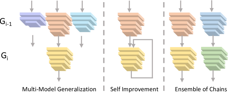
Figure 5: Sequential ensembles allows segmentation prediction conditioning between generations in various ways.

Multi-Model Generalization: Our SEQ-ENS method can be generalized to multiple architectures, where $G_{i}$ is trained to randomly condition on probability inputs $P_{i-1}$ from different $G_{0}$ segmentation models (see Fig. 5 (left)). By training a single $G_{i}$, during inference we see improved performance for all the different $G_{0}$s. In Tab. 6 we show that using HRNet-W18s [58] backbone, $G_{1}$ improves the performance of all three backbones in the HRNet family on Cityscapes and ADE20K datasets. The generalized sequential ensembles also outperforms simple ensemble baseline and have comparable performance to the default scenario of individual sequential ensembles using one-third number of parameters.

Arch	Cityscapes			ADE20K
	$G_{0}$	$G_{1}$	$G_{1}$	$G_{0}$	$G_{1}$	$G_{1}$
		Default	Generalized		Default	Generalized
H-18s	76.2	78.9	78.1	33.1	37.6	37.0
H-18	78.7	79.8	79.4	36.8	39.1	38.5
H-48	80.5	80.7	80.5	42.0	42.6	42.3

Table 6: Comparison of generalized vs default sequential ensembles using HRNet-W18s [58] backbone as $G_{1}$. Our approach allows improving performance by training $G_{1}$ models for each of the three architectures separately (default scenario). A single generalized $G_{1}$ model can give similar performance with $33\%$ parameters.

Self-Improvement: Fig. 6 (top row) shows that $G_{i}$ attempts to fix segmentation errors in the input probability map $\mathbf{P}_{i-1}$. For this example, networks improves pixel accuracy to $18.9\%$ when conditioned on a random probability map (accuracy: $1.8\%$). Interestingly, when conditioned on the ground-truth, $G_{i}$ attempts to utilize it. Inspired by this, we evaluate self-refinement as described in Fig. 5 (middle), where we feed the predicted probabilities $P_{i}$ of $G_{i}$ as its own input during inference. Tab. 7 shows non-negligible improvement in performance using self-refinement.

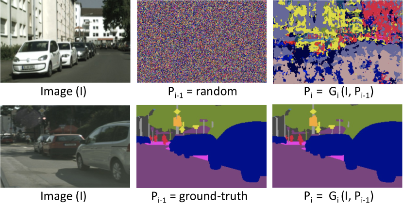
Figure 6: $\mathbf{G}_{i}$ refines/utilizes conditional probabilities $\mathbf{P}_{i-1}$. Top row shows an extreme example where $G_{i}$ refines random input probabilities. If ground-truth probabilities are provided as conditioning, $G_{i}$ utilizes them. We use this observation for self-improvement and achieve a gain of $0.6\%$ when using $3$ self-loops with HRNet-W18s backbone as shown in Tab. 7.

Arch	$\mathbf{G}_{0}$	SIM-ENS	SEQ-ENS: Self-Improvement
			$T=0$	$T=1$	$T=2$	$T=3$
H-18s	76.2	77.1	78.9	79.3	79.5	79.5
H-18	78.7	79.0	79.8	80.2	80.4	80.6
H-48	80.5	80.6	81.3	81.6	81.4	81.7

Table 7: Self-Improvement results on Cityscapes val set using single-scale inference. $T$ denotes the number of self-loops using $G_{1}$. $T=0$ represents the default sequential ensemble. Self-looping during inference provides non-negligible gains.

Ensemble of Chains: Our method allows creation of general graphs where a node is a segmentation network and the edges define the conditional dependence using the predicted probabilities. We showed that adding models/nodes in a sequential manner in a chain reduces dataset error. We can further reduce the error by adding multiple chains and averaging their predictions (Fig.5 (right)). Tab. 8 shows results on ensembling $5$ chains with varying length using MobileNetv2-D8 [52] backbone on the Cityscapes dataset.

	Number of Chains (C)
	$C=1$	$C=2$	$C=3$	$C=4$	$C=5$
$N=1$	61.3	62.2	62.4	62.7	62.7
$N=2$	64.2	65.7	66.3	65.8	66.5
$N=3$	66.1	67.2	67.4	67.8	68.1

Table 8: Multiple sequential-ensemble chains can be used to improve performance. We show performance by varying the number of chains ($C$) and the number of model generations ($N$) using MobileNetv2-D8 [52] backbone on the Cityscapes val set.

Limitations and Future Work: Sequential ensembling trains one generation at a time. This improves accuracy compared to simple ensembles, but at the cost of increased training time. Though, empirically, we observe quicker convergence for later generation when training. This is a one-time, offline cost, with potential ways to speed-up, e.g. several generations could be trained in parallel using latest prior generation predictions, possibly further reducing training time. Additional improvements could come by injecting feature maps from prior generations as inputs to future generations along with the probability map. This can further decrease the numbers of parameters required in the sequential ensemble to improve performance.

An open question for future work is whether large models give superior performance in comparison to ensembles with same number of parameters. [69] shows that ResNet-101 outperforms ResNet-152 for semantic segmentation, indicating that naïvely increasing parameters may lead to overfitting. Our sequential strategy of building complexity gradually allows training using fewer resources and enables us to modulate the accuracy vs complexity tradeoff at test time.

6 Conclusion

In this work, we explore deep ensembles to improve the performance of segmentation models. We benchmark ensembles of state-of-the-art deep models for multiple datasets. Inspired by boosting approaches, we propose sequential ensembling – a strategy to gradually increase model complexity to improve performance. This an alternative to the standard practice of training large models and compressing them for on-device deployment, and is suitable for problems with dynamic resource constraints. Our proposed ADON block utilizes feature modulation to efficiently connect multiple generations in the sequential ensemble. Sequential ensembles demonstrate state-of-the-art results on challenging datasets. We hope that our work will inspire future research in ensembling for semantic segmentation as well as other dense prediction tasks such as depth and pose estimation.

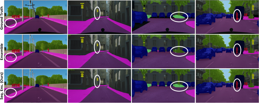
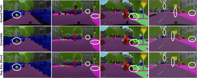
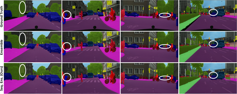
Figure 8: Qualitative comparison of Sequential Ensembles (SEQ-ENS) with the Simple Ensembles (SIM-ENS) on Cityscapes val set using HRNet-W48 backbone (N=2). The white eclipses highlight the fine-grained details that our approach captures in comparison to the baseline. Zoom in for details.

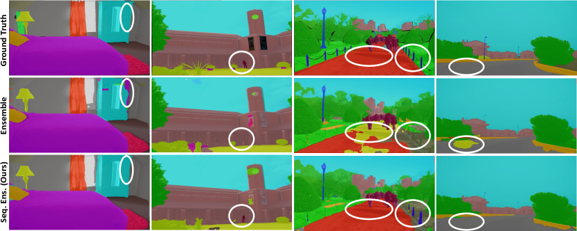
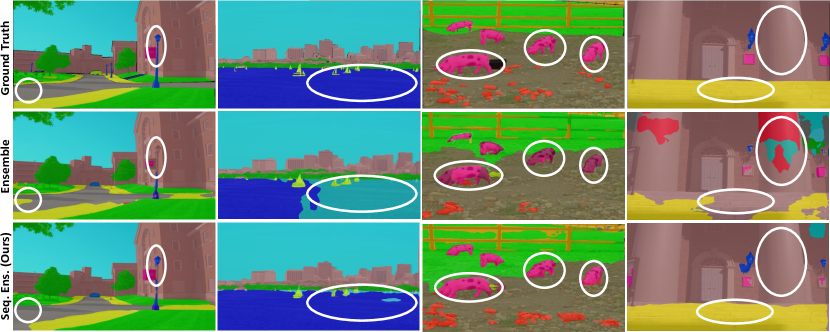
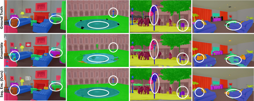
Figure 9: Qualitative comparison of Sequential Ensembles (SEQ-ENS) with the Simple Ensembles (SIM-ENS) on ADE20K val set using HRNet-W48 backbone (N=2). SEQ-ENS is especially effective on a complex dataset like ADE-20K with $150$ categories. We set a new state-of-art on ADE20K val set. Zoom in for details.

References

- [1] Vijay Badrinarayanan, Alex Kendall, and Roberto Cipolla. Segnet: A deep convolutional encoder-decoder architecture for image segmentation. IEEE transactions on pattern analysis and machine intelligence, 39(12):2481–2495, 2017.
- [2] Leo Breiman. Bagging predictors. Machine learning, 24(2):123–140, 1996.
- [3] Leo Breiman. Random forests. Machine Learning, 45:5–32, 2001.
- [4] Holger Caesar, Jasper Uijlings, and Vittorio Ferrari. Coco-stuff: Thing and stuff classes in context. In Computer vision and pattern recognition (CVPR), 2018 IEEE conference on. IEEE, 2018.
- [5] Liang-Chieh Chen, George Papandreou, Iasonas Kokkinos, Kevin Murphy, and Alan L Yuille. Deeplab: Semantic image segmentation with deep convolutional nets, atrous convolution, and fully connected crfs. IEEE transactions on pattern analysis and machine intelligence, 40(4):834–848, 2017.
- [6] Liang-Chieh Chen, George Papandreou, Florian Schroff, and Hartwig Adam. Rethinking atrous convolution for semantic image segmentation. arXiv preprint arXiv:1706.05587, 2017.
- [7] Liang-Chieh Chen, Yukun Zhu, George Papandreou, Florian Schroff, and Hartwig Adam. Encoder-decoder with atrous separable convolution for semantic image segmentation. In Proceedings of the European conference on computer vision (ECCV), pages 801–818, 2018.
- [8] Qifeng Chen and Vladlen Koltun. Photographic image synthesis with cascaded refinement networks. In Proceedings of the IEEE international conference on computer vision, pages 1511–1520, 2017.
- [9] Marius Cordts, Mohamed Omran, Sebastian Ramos, Timo Rehfeld, Markus Enzweiler, Rodrigo Benenson, Uwe Franke, Stefan Roth, and Bernt Schiele. The cityscapes dataset for semantic urban scene understanding. In Proceedings of the IEEE conference on computer vision and pattern recognition, pages 3213–3223, 2016.
- [10] Terrance DeVries and Graham W Taylor. Learning confidence for out-of-distribution detection in neural networks. arXiv preprint arXiv:1802.04865, 2018.
- [11] Philipe A Dias and Henry Medeiros. Probabilistic semantic segmentation refinement by monte carlo region growing. arXiv preprint arXiv:2005.05856, 2020.
- [12] Alexey Dosovitskiy, Lucas Beyer, Alexander Kolesnikov, Dirk Weissenborn, Xiaohua Zhai, Thomas Unterthiner, Mostafa Dehghani, Matthias Minderer, Georg Heigold, Sylvain Gelly, et al. An image is worth 16x16 words: Transformers for image recognition at scale. arXiv preprint arXiv:2010.11929, 2020.
- [13] Vincent Dumoulin, Jonathon Shlens, and Manjunath Kudlur. A learned representation for artistic style. arXiv preprint arXiv:1610.07629, 2016.
- [14] Saso Dzeroski and Bernard Zenko. Is combining classifiers better than selecting the best one? In Machine Learning, pages 255–273. Morgan Kaufmann, 2004.
- [15] Mark Everingham, SM Ali Eslami, Luc Van Gool, Christopher KI Williams, John Winn, and Andrew Zisserman. The pascal visual object classes challenge: A retrospective. International journal of computer vision, 111(1):98–136, 2015.
- [16] Stanislav Fort, Huiyi Hu, and Balaji Lakshminarayanan. Deep ensembles: A loss landscape perspective. In arXiv preprint arXiv:1912.02757, 2020.
- [17] Yoav Freund and Robert E Schapire. A decision-theoretic generalization of on-line learning and an application to boosting. Journal of computer and system sciences, 55(1):119–139, 1997.
- [18] Konrad Gadzicki, Razieh Khamsehashari, and Christoph Zetzsche. Early vs late fusion in multimodal convolutional neural networks. In 2020 IEEE 23rd International Conference on Information Fusion (FUSION), pages 1–6. IEEE, 2020.
- [19] Golnaz Ghiasi, Honglak Lee, Manjunath Kudlur, Vincent Dumoulin, and Jonathon Shlens. Exploring the structure of a real-time, arbitrary neural artistic stylization network. arXiv preprint arXiv:1705.06830, 2017.
- [20] Spyros Gidaris and Nikos Komodakis. Detect, replace, refine: Deep structured prediction for pixel wise labeling. In Proceedings of the IEEE conference on computer vision and pattern recognition, pages 5248–5257, 2017.
- [21] Kaiming He, Xiangyu Zhang, Shaoqing Ren, and Jian Sun. Deep residual learning for image recognition. In Proceedings of the IEEE conference on computer vision and pattern recognition, pages 770–778, 2016.
- [22] Andrew Howard, Mark Sandler, Grace Chu, Liang-Chieh Chen, Bo Chen, Mingxing Tan, Weijun Wang, Yukun Zhu, Ruoming Pang, Vijay Vasudevan, et al. Searching for mobilenetv3. In Proceedings of the IEEE/CVF International Conference on Computer Vision, pages 1314–1324, 2019.
- [23] Jie Hu, Li Shen, and Gang Sun. Squeeze-and-excitation networks. In Proceedings of the IEEE conference on computer vision and pattern recognition, pages 7132–7141, 2018.
- [24] Gao Huang, Yixuan Li, Geoff Pleiss, Zhuang Liu, John E Hopcroft, and Kilian Q Weinberger. Snapshot ensembles: Train 1, get m for free. arXiv preprint arXiv:1704.00109, 2017.
- [25] Xun Huang and Serge Belongie. Arbitrary style transfer in real-time with adaptive instance normalization. In Proceedings of the IEEE International Conference on Computer Vision, pages 1501–1510, 2017.
- [26] Zilong Huang, Xinggang Wang, Lichao Huang, Chang Huang, Yunchao Wei, and Wenyu Liu. Ccnet: Criss-cross attention for semantic segmentation. In Proceedings of the IEEE/CVF International Conference on Computer Vision, pages 603–612, 2019.
- [27] Sergey Ioffe and Christian Szegedy. Batch normalization: Accelerating deep network training by reducing internal covariate shift. In International conference on machine learning, pages 448–456. PMLR, 2015.
- [28] Md Amirul Islam, Shujon Naha, Mrigank Rochan, Neil Bruce, and Yang Wang. Label refinement network for coarse-to-fine semantic segmentation. arXiv preprint arXiv:1703.00551, 2017.
- [29] Shun Iwase, Xingyu Liu, Rawal Khirodkar, Rio Yokota, and Kris M Kitani. Repose: Fast 6d object pose refinement via deep texture rendering. In Proceedings of the IEEE/CVF International Conference on Computer Vision, pages 3303–3312, 2021.
- [30] Shruti Jadon. A survey of loss functions for semantic segmentation. In 2020 IEEE Conference on Computational Intelligence in Bioinformatics and Computational Biology (CIBCB), pages 1–7. IEEE, 2020.
- [31] Rawal Khirodkar, Visesh Chari, Amit Agrawal, and Ambrish Tyagi. Multi-hypothesis pose networks: Rethinking top-down pose estimation. arXiv preprint arXiv:2101.11223, 2021.
- [32] Rawal Khirodkar and Kris M Kitani. Adversarial domain randomization. arXiv preprint arXiv:1812.00491, 2018.
- [33] Rawal Khirodkar, Shashank Tripathi, and Kris Kitani. Occluded human mesh recovery. In Proceedings of the IEEE/CVF Conference on Computer Vision and Pattern Recognition, pages 1715–1725, 2022.
- [34] Rawal Khirodkar, Donghyun Yoo, and Kris Kitani. Domain randomization for scene-specific car detection and pose estimation. In 2019 IEEE Winter Conference on Applications of Computer Vision (WACV), pages 1932–1940. IEEE, 2019.
- [35] Taesup Kim, Inchul Song, and Yoshua Bengio. Dynamic layer normalization for adaptive neural acoustic modeling in speech recognition. arXiv preprint arXiv:1707.06065, 2017.
- [36] Diederik P Kingma and Jimmy Ba. Adam: A method for stochastic optimization. arXiv preprint arXiv:1412.6980, 2014.
- [37] Alex Krizhevsky, Ilya Sutskever, and Geoffrey E Hinton. Imagenet classification with deep convolutional neural networks. Advances in neural information processing systems, 25:1097–1105, 2012.
- [38] Weicheng Kuo, Anelia Angelova, Jitendra Malik, and Tsung-Yi Lin. Shapemask: Learning to segment novel objects by refining shape priors. In Proceedings of the IEEE/CVF International Conference on Computer Vision, pages 9207–9216, 2019.
- [39] Balaji Lakshminarayanan, Alexander Pritzel, and Charles Blundell. Simple and scalable predictive uncertainty estimation using deep ensembles. In Proceedings of the 31st Conference on Neural Information Processing Systems (NeurIPS), 2017.
- [40] Ke Li, Bharath Hariharan, and Jitendra Malik. Iterative instance segmentation. In Proceedings of the IEEE conference on computer vision and pattern recognition, pages 3659–3667, 2016.
- [41] Yanwei Li, Lin Song, Yukang Chen, Zeming Li, Xiangyu Zhang, Xingang Wang, and Jian Sun. Learning dynamic routing for semantic segmentation. In Proceedings of the IEEE/CVF Conference on Computer Vision and Pattern Recognition, pages 8553–8562, 2020.
- [42] Guosheng Lin, Anton Milan, Chunhua Shen, and Ian Reid. Refinenet: Multi-path refinement networks for high-resolution semantic segmentation. In Proceedings of the IEEE conference on computer vision and pattern recognition, pages 1925–1934, 2017.
- [43] Janice Lin, Wen-June Wang, Sheng-Kai Huang, and Hsiang-Chieh Chen. Learning based semantic segmentation for robot navigation in outdoor environment. In 2017 Joint 17th World Congress of International Fuzzy Systems Association and 9th International Conference on Soft Computing and Intelligent Systems (IFSA-SCIS), pages 1–5. IEEE, 2017.
- [44] Ze Liu, Yutong Lin, Yue Cao, Han Hu, Yixuan Wei, Zheng Zhang, Stephen Lin, and Baining Guo. Swin transformer: Hierarchical vision transformer using shifted windows. arXiv preprint arXiv:2103.14030, 2021.
- [45] Jonathan Long, Evan Shelhamer, and Trevor Darrell. Fully convolutional networks for semantic segmentation. In Proceedings of the IEEE conference on computer vision and pattern recognition, pages 3431–3440, 2015.
- [46] Yuyi Mao, Jun Zhang, and Khaled B Letaief. Dynamic computation offloading for mobile-edge computing with energy harvesting devices. IEEE Journal on Selected Areas in Communications, 34(12):3590–3605, 2016.
- [47] Gyeongsik Moon, Ju Yong Chang, and Kyoung Mu Lee. Posefix: Model-agnostic general human pose refinement network. In Proceedings of the IEEE/CVF Conference on Computer Vision and Pattern Recognition, pages 7773–7781, 2019.
- [48] Roozbeh Mottaghi, Xianjie Chen, Xiaobai Liu, Nam-Gyu Cho, Seong-Whan Lee, Sanja Fidler, Raquel Urtasun, and Alan Yuille. The role of context for object detection and semantic segmentation in the wild. In IEEE Conference on Computer Vision and Pattern Recognition (CVPR), 2014.
- [49] Ethan Perez, Florian Strub, Harm De Vries, Vincent Dumoulin, and Aaron Courville. Film: Visual reasoning with a general conditioning layer. In Proceedings of the AAAI Conference on Artificial Intelligence, volume 32, 2018.
- [50] Olaf Ronneberger, Philipp Fischer, and Thomas Brox. U-net: Convolutional networks for biomedical image segmentation. In International Conference on Medical image computing and computer-assisted intervention, pages 234–241. Springer, 2015.
- [51] Sebastian Ruder. An overview of gradient descent optimization algorithms. arXiv preprint arXiv:1609.04747, 2016.
- [52] Mark Sandler, Andrew Howard, Menglong Zhu, Andrey Zhmoginov, and Liang-Chieh Chen. Mobilenetv2: Inverted residuals and linear bottlenecks. In Proceedings of the IEEE conference on computer vision and pattern recognition, pages 4510–4520, 2018.
- [53] Robert E Schapire. The strength of weak learnability. Machine learning, 5(2):197–227, 1990.
- [54] Robert E Schapire and Yoav Freund. A decision-theoretic generalization of on-line learning and an application to boosting. In Second European Conference on Computational Learning Theory, pages 23–37, 1995.
- [55] Jamie Shotton, John Winn, Carsten Rother, and Antonio Criminisi. Textonboost for image understanding: Multi-class object recognition and segmentation by jointly modeling texture, layout, and context. International journal of computer vision, 81(1):2–23, 2009.
- [56] Mennatullah Siam, Sara Elkerdawy, Martin Jagersand, and Senthil Yogamani. Deep semantic segmentation for automated driving: Taxonomy, roadmap and challenges. In 2017 IEEE 20th international conference on intelligent transportation systems (ITSC), pages 1–8. IEEE, 2017.
- [57] Karen Simonyan and Andrew Zisserman. Very deep convolutional networks for large-scale image recognition. arXiv preprint arXiv:1409.1556, 2014.
- [58] Ke Sun, Yang Zhao, Borui Jiang, Tianheng Cheng, Bin Xiao, Dong Liu, Yadong Mu, Xinggang Wang, Wenyu Liu, and Jingdong Wang. High-resolution representations for labeling pixels and regions. arXiv preprint arXiv:1904.04514, 2019.
- [59] Christian Szegedy, Wei Liu, Yangqing Jia, Pierre Sermanet, Scott Reed, Dragomir Anguelov, Dumitru Erhan, Vincent Vanhoucke, and Andrew Rabinovich. Going deeper with convolutions. In Proceedings of the IEEE conference on computer vision and pattern recognition, pages 1–9, 2015.
- [60] Towaki Takikawa, David Acuna, Varun Jampani, and Sanja Fidler. Gated-scnn: Gated shape cnns for semantic segmentation. In Proceedings of the IEEE/CVF International Conference on Computer Vision, pages 5229–5238, 2019.
- [61] Mingxing Tan and Quoc Le. Efficientnet: Rethinking model scaling for convolutional neural networks. In International Conference on Machine Learning, pages 6105–6114. PMLR, 2019.
- [62] Paul Viola and Michael Jones. Rapid object detection using a boosted cascade of simple features. In Proceedings of the 2001 IEEE computer society conference on computer vision and pattern recognition. CVPR 2001, volume 1, pages I–I. Ieee, 2001.
- [63] Huiyu Wang, Yukun Zhu, Bradley Green, Hartwig Adam, Alan Yuille, and Liang-Chieh Chen. Axial-deeplab: Stand-alone axial-attention for panoptic segmentation. In European Conference on Computer Vision, pages 108–126. Springer, 2020.
- [64] Jingdong Wang, Ke Sun, Tianheng Cheng, Borui Jiang, Chaorui Deng, Yang Zhao, Dong Liu, Yadong Mu, Mingkui Tan, Xinggang Wang, et al. Deep high-resolution representation learning for visual recognition. IEEE transactions on pattern analysis and machine intelligence, 2020.
- [65] Xiaofang Wang, Dan Kondratyuk, Eric Christiansen, Kris M Kitani, Yair Movshovitz-Attias, and Elad Eban. On the surprising efficiency of committee-based models. arXiv preprint arXiv:2012.01988, 2020.
- [66] Yeming Wen, Dustin Tran, and Jimmy Ba. Batchensemble: an alternative approach to efficient ensemble and lifelong learning. arXiv preprint arXiv:2002.06715, 2020.
- [67] Florian Wenzel, Jasper Snoek, Dustin Tran, and Rodolphe Jenatton. Hyperparameter ensembles for robustness and uncertainty quantification. arXiv preprint arXiv:2006.13570, 2020.
- [68] David H. Wolpert. Neural Networks, 5, 1992.
- [69] Zifeng Wu, Chunhua Shen, and Anton van den Hengel. High-performance semantic segmentation using very deep fully convolutional networks. arXiv preprint arXiv:1604.04339, 2016.
- [70] Zifeng Wu, Chunhua Shen, and Anton Van Den Hengel. Wider or deeper: Revisiting the resnet model for visual recognition. Pattern Recognition, 90:119–133, 2019.
- [71] Enze Xie, Wenhai Wang, Zhiding Yu, Anima Anandkumar, Jose M Alvarez, and Ping Luo. Segformer: Simple and efficient design for semantic segmentation with transformers. arXiv preprint arXiv:2105.15203, 2021.
- [72] Fisher Yu and Vladlen Koltun. Multi-scale context aggregation by dilated convolutions. arXiv preprint arXiv:1511.07122, 2015.
- [73] Fisher Yu, Vladlen Koltun, and Thomas Funkhouser. Dilated residual networks. In Proceedings of the IEEE conference on computer vision and pattern recognition, pages 472–480, 2017.
- [74] Yuhui Yuan, Xilin Chen, and Jingdong Wang. Object-contextual representations for semantic segmentation. In Computer Vision–ECCV 2020: 16th European Conference, Glasgow, UK, August 23–28, 2020, Proceedings, Part VI 16, pages 173–190. Springer, 2020.
- [75] Yuhui Yuan, Jingyi Xie, Xilin Chen, and Jingdong Wang. Segfix: Model-agnostic boundary refinement for segmentation. In European Conference on Computer Vision, pages 489–506. Springer, 2020.
- [76] Hang Zhang, Kristin Dana, Jianping Shi, Zhongyue Zhang, Xiaogang Wang, Ambrish Tyagi, and Amit Agrawal. Context encoding for semantic segmentation. In Proceedings of the IEEE conference on Computer Vision and Pattern Recognition, pages 7151–7160, 2018.
- [77] Hengshuang Zhao, Jianping Shi, Xiaojuan Qi, Xiaogang Wang, and Jiaya Jia. Pyramid scene parsing network. In Proceedings of the IEEE conference on computer vision and pattern recognition, pages 2881–2890, 2017.
- [78] Ying Zhao, Jun Gao, and Xuezhi Yang. A survey of neural network ensembles. In 2005 International Conference on Neural Networks and Brain, volume 1, pages 438–442. IEEE, 2005.
- [79] Sixiao Zheng, Jiachen Lu, Hengshuang Zhao, Xiatian Zhu, Zekun Luo, Yabiao Wang, Yanwei Fu, Jianfeng Feng, Tao Xiang, Philip HS Torr, et al. Rethinking semantic segmentation from a sequence-to-sequence perspective with transformers. In Proceedings of the IEEE/CVF Conference on Computer Vision and Pattern Recognition, pages 6881–6890, 2021.
- [80] Bolei Zhou, Hang Zhao, Xavier Puig, Sanja Fidler, Adela Barriuso, and Antonio Torralba. Scene parsing through ade20k dataset. In Proceedings of the IEEE Conference on Computer Vision and Pattern Recognition, 2017.
- [81] Bolei Zhou, Hang Zhao, Xavier Puig, Tete Xiao, Sanja Fidler, Adela Barriuso, and Antonio Torralba. Semantic understanding of scenes through the ade20k dataset. International Journal of Computer Vision, 127(3):302–321, 2019.