A randomized operator splitting scheme inspired by stochastic optimization methods

Abstract.

In this paper, we combine the operator splitting methodology for abstract evolution equations with that of stochastic methods for large-scale optimization problems. The combination results in a randomized splitting scheme, which in a given time step does not necessarily use all the parts of the split operator. This is in contrast to deterministic splitting schemes which always use every part at least once, and often several times. As a result, the computational cost can be significantly decreased in comparison to such methods. We rigorously define a randomized operator splitting scheme in an abstract setting and provide an error analysis where we prove that the temporal convergence order of the scheme is at least $1/2$. We illustrate the theory by numerical experiments on both linear and quasilinear diffusion problems, using a randomized domain decomposition approach. We conclude that choosing the randomization in certain ways may improve the order to $1$. This is as accurate as applying e.g. backward (implicit) Euler to the full problem, without splitting.

1. Introduction

The main objective of this paper is to combine two successful strategies from the literature: the first being operator splitting schemes for evolution equations on general, infinite dimensional frameworks and the second being stochastic optimization methods. Operator splitting schemes are an established tool in the field of numerical analysis of evolution equations and have a wide range of applications. Stochastic optimization methods have proven to be efficient at solving large-scale optimization problems, where it is infeasible to evaluate full gradients. They can drastically decrease the computational cost in e.g. machine learning settings. The link between these two seemingly disparate areas is that an iterative method applied to an optimization problem can also be seen as a time-stepping method applied to a gradient flow connected to the optimization problem. In particular, stochastic optimization methods can then be interpreted as randomized operator splitting schemes for such gradient flows. In this context, we introduce a general randomized splitting method that can be applied directly to evolution equations, and provide a rigorous convergence analysis.

Abstract evolution equations of the type

$$\begin{cases}u^{\prime}(t)+A(t)u(t)=f(t),\quad t\in(0,T],\\ u(0)=u_{0}\end{cases}$$

are an important building block for modeling processes in physics, biology and social sciences. Standard examples which appear in a variety of applications are fluid flow problems, where we model how a flow evolves on a given domain over time, compare [1, 26] and [37, Section 1.3]. The operator $A(t)$ can denote, for example, a non-linear diffusion operator such as the $p$-Laplacian or a porous medium operator.

Deterministic operator splitting schemes as discussed in more detail in [16] are a powerful tool for this type of equation. An example is given by a domain decomposition scheme, where we split the domain into sub-domains. Instead of solving one expensive problem on the entire domain, we deal with cheaper problems on the sub-domains. This is particularly useful in modern computer architectures, as the sub-problems may often be solved in parallel.

Moreover, evolution equations are tightly connected to unconstrained optimization problems, because the solution of $\min_{u}F(u)$ is a stationary point of the gradient flow $u^{\prime}(t)=-\nabla F(u(t))$. The latter is an evolution equation on an infinite time horizon with $A=-\nabla F$ and $f=0$. In the large-scale case, such optimization problems benefit from stochastic optimization schemes. The most basic such method, the stochastic gradient descent, was first introduced already in [32], but since then it has been extended and generalized in many directions. See, e.g., the review article [3] and the references therein.

Via the gradient flow interpretation, we can see these optimization methods as time-stepping schemes where a randomly chosen sub-problem is considered in each time step. In essence, it is therefore a randomized operator splitting scheme. The difference between the works mentioned above and ours is that we apply these stochastic optimization techniques to solve the evolution equation itself rather than just finding its stationary state.

We consider nonlinear evolution equations in an abstract framework similar to [7, 10, 11] where operators of a monotone type have been studied. Deterministic splitting schemes for such equations has been considered in e.g. [14, 15, 17, 29]. A particular kind of splitting schemes which is most closely related to our work, domain decomposition methods, have been studied in [6, 7, 13, 30, 31]. In this paper, we extend this framework of deterministic splitting schemes to a setting of randomized methods.

Outside of the context of optimization, other kinds of randomized methods have already proved themselves to be useful for solving evolution equations. Starting in [34, 35] explicit schemes for ordinary differential equations have been randomized. This approach has been further extended in [2, 4, 18, 22, 24]. In [8], it has been extended both to implicit methods and to partial differential equations and in [23] to finite element approximations. While these works considered certain randomizations in their schemes, they are conceptually different from our approach. Their main idea is to approximate any appearing integrals through

$$\int_{t_{n-1}}^{t_{n}}f(t)\,\mathrm{d}t\approx f(\xi_{n})\quad\text{and}\quad\int_{t_{n-1}}^{t_{n}}A(t)v\,\mathrm{d}t\approx A(\xi_{n})v,$$

where $\xi_{n}$ is a random variable that takes on values in $[t_{n-1},t_{n}]$. This ansatz coincides with a Monte Carlo integration idea. In this paper, we use a different approach where we decompose the operator in a randomized fashion. More precisely, we approximate data

$$f=\frac{1}{s}\sum_{\ell=1}^{s}f_{\ell}\quad\text{and}\quad A=\frac{1}{s}\sum_{\ell=1}^{s}A_{\ell}$$

by

$$f_{B}=\frac{1}{|B|}\sum_{\ell\in B}f_{\ell}\quad\text{and}\quad A_{B}=\frac{1}{|B|}\sum_{\ell\in B}A_{\ell}$$

where the batch $B\subset\{1,\dots,s\}$ is chosen randomly. The stochastic approximations $f_{B}$ and $A_{B}$ of the original data $f$ and $A$ are cheaper to evaluate in applications. This is less related to Monte Carlo integration and more similar to stochastic optimization methods, compare [3, 9]. Similar ideas have been considered in [19, 20, 28], where a random batch method for interacting particle systems has been studied. Moreover, very recently and during the preparation of this work, a similar approach has also been applied to the optimal control of linear time invariant (LTI) dynamical systems in [38]. While the convergence rate provided there is essentially the same as what we establish in our main result Theorem 5.2, our setting is more general and allows for nonlinear operators on infinite dimensional spaces rather than finite dimensional matrices. We also consider the error of the time stepping method that is used to approximate the solution to $u^{\prime}(t)+A_{B}(t)u(t)=f_{B}(t)$, while the error bounds in [38] assume that this evolution equation is solved exactly.

This paper is organized as follows. In Section 2, we begin by explaining our abstract framework. This includes both the precise assumptions that we make and the definition of our time-stepping scheme. We give a more concrete application of the abstract framework in Section 3. With the setting fixed, we first prove in Section 4 that the scheme and its solution are indeed well-defined. We prove the convergence of the scheme in expectation in Section 5. These theoretical convergence results are illustrated by numerical experiments with two-dimensional linear and quasilinear nonlinear and linear diffusion problem in Section 6. Finally, we collect some more technical auxiliary results in Appendix A.

2. Setting

In the following, we introduce a theoretical framework for the randomized operator splitting. This setting is similar to the one in [7].

Assumption 1.

Let $(H,(\cdot,\cdot)_{H},\|\cdot\|_{H})$ be a real, separable Hilbert space and let $(V,\|\cdot\|_{V})$ be a real, separable, reflexive Banach space, which is continuously and densely embedded into $H$. Moreover, there exists a semi-norm $|\cdot|_{V}$ on $V$.

Denoting the dual space of $V$ by $V^{*}$ and identifying the Hilbert space $H$ with its dual space, the spaces from Assumption 1 form a Gelfand triple and fulfill, in particular,

$$V\overset{d}{\hookrightarrow}H\cong H^{*}\overset{d}{\hookrightarrow}V^{*}.$$

Assumption 2.

Let the spaces $H$ and $V$ be given as stated in Assumption 1. Furthermore, for $T\in(0,\infty)$ as well as $p\in[2,\infty)$, let $\{A(t)\}_{t\in[0,T]}$ be a family of operators $A(t)\colon V\to V^{*}$ that satisfy the following conditions:

1. The mapping $Av\colon[0,T]\to V^{*}$ given by $t\mapsto A(t)v$ is continuous almost everywhere in $(0,T)$ for all $v\in V$.

2. The operator $A(t)\colon V\to V^{*}$, $t\in[0,T]$, is radially continuous, i.e., the mapping $s\mapsto\langle A(t)(v+sw),w\rangle_{V^{*}\times V}$ is continuous on $[0,1]$ for all $v,w\in V$.

3. For $\kappa_{A}\in[0,\infty)$, the operator $A(t)+\kappa_{A}I\colon V\to V^{*}$, $t\in[0,T]$, fulfills a monotonicity-type condition in the sense that there exists $\eta_{A}\in[0,\infty)$, which does not depend on $t$, such that

   $$\langle A(t)v-A(t)w,v-w\rangle_{V^{*}\times V}+\kappa_{A}\|v-w\|_{H}^{2}\geq\eta_{A}|v-w|_{V}^{p}$$

   is fulfilled for all $v,w\in V$.

4. The operator $A(t)\colon V\to V^{*}$, $t\in[0,T]$, is uniformly bounded such that there exists $\beta_{A}\in[0,\infty)$, which does not depend on $t$, with

   $$\|A(t)v\|_{V^{*}}\leq\beta_{A}\big{(}1+\|v\|_{V}^{p-1}\big{)}$$

   for all $v\in V$.

5. The operator $A(t)+\kappa_{A}I\colon V\to V^{*}$, $t\in[0,T]$, fulfills a uniform semi-coercivity condition such that there exist $\mu_{A},\lambda_{A}\in[0,\infty)$, which do not depend on $t$, with

   $$\langle A(t)v,v\rangle_{V^{*}\times V}+\kappa_{A}\|v\|_{H}^{2}+\lambda_{A}\geq\mu_{A}|v|_{V}^{p}$$

   for all $v\in V$.

Assumption 3.

The function $f$ is an element of the Bochner space $L^{2}(0,T;H)$, and the initial value $u_{0}\in H$, where $H$ is the Hilbert space from Assumption 1.

Assumption 1–3, are requirements on the problem that we want to solve. The following Assumptions 4–5 are needed to state the approximation scheme for the given problem.

Assumption 4.

Let $(\Omega,\mathcal{F},\mathcal{P})$ be a complete probability space and let $\{\xi_{n}\}_{n\in\mathbb{N}}$ be a family of mutually independent random variables. Further, let the filtration $\{\mathcal{F}_{n}\}_{n\in\mathbb{N}}$ be given by

$$\mathcal{F}_{0}:=\sigma\big{(}\mathcal{N}\in\mathcal{F}:\mathcal{P}(\mathcal{N})=0\big{)}$$

$$\mathcal{F}_{n}:=\sigma\big{(}\sigma\big{(}\xi_{i}:i\in\{1,\dots,n\}\big{)}\cup\mathcal{F}_{0}\big{)},\quad n\in\mathbb{N},$$

where $\sigma$ denotes the generated $\sigma$-algebra.

In the following, we denote the expectation with respect to the probability distribution of $\xi$ for a random variable $X$ in the Bochner space $L^{1}(\Omega;H)$ by $\mathbb{E}_{\xi}[X]$. Moreover, we abbreviate the total expectation by

$$\mathbb{E}_{n}[X]=\mathbb{E}_{\xi_{1}}[\mathbb{E}_{\xi_{2}}[\dots\mathbb{E}_{\xi_{n}}[X]\dots]].$$

We denote the space of Hölder continuous functions on $[0,T]$ with Hölder coefficient $\gamma\in(0,1)$ and values in $H$ by $C^{\gamma}([0,T];H)$. For notational convenience we include the case $\gamma=1$ and denote the space of Lipschitz continuous functions by $C^{1}([0,T];H)$.

Assumption 5.

Let Assumptions 1–4 be fulfilled. Assume that for almost every $\omega\in\Omega$, there exists a real Banach space $V_{\xi(\omega)}$ such that $V\stackrel{{\scriptstyle d}}{{\hookrightarrow}}V_{\xi(\omega)}\stackrel{{\scriptstyle d}}{{\hookrightarrow}}H$, $\bigcap_{\omega\in\Omega}V_{\xi(\omega)}=V$ and there exists a semi-norm $|\cdot|_{V_{\xi(\omega)}}$. Moreover, the mapping from $\omega\mapsto V_{\xi(\omega)}$ is measurable in the sense that for every $v\in H$ the set $\{\omega\in\Omega:v\in V_{\xi(\omega)}\}$ is an element of the complete generated $\sigma$-algebra

$$\mathcal{F}_{\xi}:=\sigma\big{(}\sigma(\xi)\cup\sigma\big{(}\mathcal{N}\in\mathcal{F}:\mathcal{P}(\mathcal{N})=0\big{)}\big{)}.$$

Further, let the family of operators $\{A_{\xi(\omega)}(t)\}_{\omega\in\Omega,t\in[0,T]}$ be such that for almost every $\omega\in\Omega$, $\{A_{\xi(\omega)}(t)\}_{t\in[0,T]}$ fulfills Assumption 2 with the spaces $V_{\xi(\omega)}$, $H$ and $V_{\xi(\omega)}^{*}$ and corresponding constants $\kappa_{\xi(\omega)}$, $\eta_{\xi(\omega)}$, $\beta_{\xi(\omega)}$, $\mu_{\xi(\omega)}$ and $\lambda_{\xi(\omega)}$. Moreover, the mapping $A_{\xi}(t)v\colon\Omega\to V^{*}$ is $\mathcal{F}_{\xi}$-measurable and the equality $\mathbb{E}_{\xi}[A_{\xi}(t)v]=A(t)v$ is fulfilled in $V^{*}$ for $v\in V$. The mappings $\kappa_{\xi},\eta_{\xi},\mu_{\xi},\beta_{\xi},\lambda_{\xi}\colon\Omega\to[0,\infty)$ are measurable and there exist $\kappa,\lambda\in[0,\infty)$ which fulfill $\kappa_{\xi}\leq\kappa$ almost surely and $\mathbb{E}_{\xi}\big{[}\lambda_{\xi}\big{]}\leq\lambda$.

Further, let the family $\{f_{\xi(\omega)}\}_{\omega\in\Omega}$ be given such that $f_{\xi(\omega)}\in L^{2}(0,T;H)$. Moreover, the mapping $f_{\xi}(t)\colon\Omega\to H$ is $\mathcal{F}_{\xi}$-measurable and $\mathbb{E}_{\xi}[f_{\xi}(t)]=f(t)$ is fulfilled in $H$ for almost all $t\in(0,T)$.

Under the setting explained in the above assumptions, we consider the initial value problem

(2.1) $$\begin{cases}u^{\prime}(t)+A(t)u(t)=f(t)\quad&\text{in }V^{*},\quad t\in(0,T],\\ u(0)=u_{0}&\text{in }H.\end{cases}$$

For a non-uniform temporal grid $0=t_{0}<t_{1}<\dots<t_{N}=T$, a step size $h_{n}=t_{n}-t_{n-1}$, $h=\max_{n\in\{1,\dots,N\}}h_{n}$, and a family of random variables $\{f^{n}\}_{n\in\{1,\dots,N\}}$ such that $f^{n}\colon\Omega\to H$ is $\mathcal{F}_{\xi_{n}}$-measurable, we consider the scheme

(2.2) $$\begin{cases}U^{n}-U^{n-1}+h_{n}A_{\xi_{n}}(t_{n})U^{n}=h_{n}f^{n}\quad&\text{in }V_{\xi_{n}}^{*},\quad n\in\{1,\dots,N\},\\ U^{0}=u_{0}&\text{in }H.\end{cases}$$

Note that $U^{n}\colon\Omega\to H$ is a random variable and therefore some statements involving it below only hold almost surely. Whenever there is no risk of misinterpretation, we omit writing almost surely for the sake of brevity.

When proving that the scheme is well-defined and establishing an a priori bound, it is sufficient to assume that $\{f_{\xi_{n}}\}_{n\in\{1,\dots,N\}}$ are integrable with respect to the temporal parameter. In that case, we can choose for example

(2.3) $$f^{n}=\frac{1}{h_{n}}\int_{t_{n-1}}^{t_{n}}f_{\xi_{n}}(t)\,\mathrm{d}t\quad\text{in }H\text{ almost surely.}$$

In our error bounds, we assume more regularity for the functions $\{f_{\xi_{n}}\}_{n\in\{1,\dots,N\}}$ and demand continuity with respect to the temporal parameter. In this case, we may also use

(2.4) $$f^{n}=f_{\xi_{n}}(t_{n})\quad\text{in }H\text{ almost surely.}$$

We will focus on this second choice for the error bounds in Section 5.

3. Application: Domain decomposition

One main application that is allowed by our abstract framework is a domain decomposition scheme for a nonlinear fluid flow problem. Domain decomposition schemes are well-known for deterministic operator splittings. However, to the best of our knowledge, it has not been studied in the context of a randomized operator splitting scheme.

3.1. Deterministic domain decomposition

To exemplify our abstract equation (2.1), we consider a (nonlinear) parabolic differential equation. In the following, let $\mathcal{D}\subset\mathbb{R}^{d}$, $d\in\mathbb{N}$, be a bounded domain with a Lipschitz boundary $\partial\mathcal{D}$. For $p\in[2,\infty)$, we consider the parabolic $p$-Laplacian with homogeneous Dirichlet boundary conditions

(3.1) $$\begin{cases}\partial_{t}u(t,x)-\nabla\cdot(\alpha(t)|\nabla u(t,x)|^{p-2}\nabla u(t,x))=\tilde{f}(t,x),\quad&(t,x)\in(0,T)\times\mathcal{D},\\ u(t,x)=0,&(t,x)\in(0,T)\times\partial\mathcal{D},\\ u(0,x)=u_{0}(x),&x\in\mathcal{D},\end{cases}$$

for $\alpha\colon[0,T]\to\mathbb{R}$ and $u_{0}\colon\mathcal{D}\to\mathbb{R}$. The notation $\tilde{f}$ is used to differentiate between the function $\tilde{f}\colon(0,T)\times\mathcal{D}\to\mathbb{R}$ and the abstract function $f$ on $(0,T)$ that it gives rise to through $[f(t)](x)=\tilde{f}(t,x)$. We consider a domain decomposition scheme similar to [13] for $p=2$ and to [6, 7] for $p\in[2,\infty)$. For the sake of completeness, we recapitulate the setting here also with a different boundary condition.

For $s\in\mathbb{N}$, let $\{\mathcal{D}_{\ell}\}_{\ell=1}^{s}$ be a family of overlapping subsets of $\mathcal{D}$. Let each subset have a Lipschitz boundary and let the union of them fulfill $\bigcup_{\ell=1}^{s}\mathcal{D}_{\ell}=\mathcal{D}$. On the sub-domains $\{\mathcal{D}_{\ell}\}_{\ell=1}^{s}$, let the partition of unity $\{\chi_{\ell}\}_{\ell=1}^{s}\subset W^{1,\infty}(\mathcal{D})$ be given such that the following criteria are fulfilled

$$\chi_{\ell}(x)>0\text{ for all }x\in\mathcal{D}_{\ell},\quad\chi_{\ell}(x)=0\text{ for all }x\in\mathcal{D}\setminus\mathcal{D}_{\ell},\quad\sum_{\ell=1}^{s}\chi_{\ell}=1$$

for $\ell\in\{1,\dots,s\}$. With the help of the functions $\{\chi_{\ell}\}_{\ell\in\{1,\dots,s\}}$, it is now possible to introduce suitable functional spaces $\{V_{\ell}\}_{\ell\in\{1,\dots,s\}}$. We use the weighted Lebesgue space $L^{p}(\mathcal{D}_{\ell},\chi_{\ell})^{d}$ that consists of all measurable functions $v=(v_{1},\dots,v_{d})\colon\mathcal{D}_{\ell}\to\mathbb{R}^{d}$ such that

$$\|(v_{1},\ldots,v_{d})\|_{L^{p}(\mathcal{D}_{\ell},\chi_{\ell})^{d}}=\Big{(}\int_{\mathcal{D}_{\ell}}\chi_{\ell}|(v_{1},\ldots,v_{d})|^{p}\,\mathrm{d}x\Big{)}^{\frac{1}{p}}$$

is finite. In the following, let the pivot space $\left(H,(\cdot,\cdot)_{H},\|\cdot\|_{H}\right)$ be the space $L^{2}(\mathcal{D})$ of square integrable functions on $\mathcal{D}$ with the usual norm and inner product. The spaces $V$ and $V_{\ell}$, $\ell\in\{1,\dots,s\}$, are given by

$$V=\text{clos}_{\|\cdot\|_{V}}\big{(}C_{0}^{\infty}(\mathcal{D})\big{)}=W_{0}^{1,p}(\mathcal{D})\quad\text{and}\quad V_{\ell}=\text{clos}_{\|\cdot\|_{V_{\ell}}}\big{(}C_{0}^{\infty}(\mathcal{D})\big{)},$$

with respect to the norms

(3.2) $$\|\cdot\|_{V}=\|\cdot\|_{H}+\|\nabla\cdot\|_{L^{p}(\mathcal{D})^{d}}\quad\text{and}\quad\|\cdot\|_{V_{\ell}}=\|\cdot\|_{H}+\|\nabla\cdot\|_{L^{p}(\mathcal{D}_{\ell},\chi_{\ell})^{d}}$$

and semi-norms

$$|\cdot|_{V}=\|\nabla\cdot\|_{L^{p}(\mathcal{D})^{d}}\quad\text{and}\quad|\cdot|_{V_{\ell}}=\|\nabla\cdot\|_{L^{p}(\mathcal{D}_{\ell},\chi_{\ell})^{d}}.$$

Note that a bootstrap argument involving the Sobolev embedding theorem shows that the norm given in (3.2) is equivalent to the standard norm in the space. We can now introduce the operators $A(t)\colon V\to V^{*}$, $A_{\ell}(t)\colon V_{\ell}\to V^{*}_{\ell}$, $\ell\in\{1,\dots,s\}$, $t\in[0,T]$, given by

$$\langle A(t)u,v\rangle_{V^{*}\times V} =\int_{\mathcal{D}}\alpha(t)|\nabla u|^{p-2}\nabla u\cdot\nabla v\,\mathrm{d}x,\quad u,v\in V,$$

$$\langle A_{\ell}(t)u,v\rangle_{V_{\ell}^{*}\times V_{\ell}} =\int_{\mathcal{D}_{\ell}}\chi_{\ell}\alpha(t)|\nabla u|^{p-2}\nabla u\cdot\nabla v\,\mathrm{d}x,\quad u,v\in V_{\ell}.$$

Similarly, we define the right-hand sides $f_{\ell}\colon[0,T]\to H$, $\ell\in\{1,\dots,s\}$, where $f_{\ell}(t)=\chi_{\ell}f(t)$ in $H$ for almost every $t\in(0,T)$.

Lemma 3.1.

Let the parameters of the equation (3.1) be given such that $\alpha\in C([0,T];\mathbb{R})$, $u_{0}\in L^{2}(\mathcal{D})$ and $\tilde{f}\in L^{2}((0,T)\times\mathcal{D})$. Then the setting described above fulfills Assumptions 1–3.

Let the partition of unity $\{\chi_{\ell}\}_{\ell=1}^{s}\subset W^{1,\infty}(\mathcal{D})$ fulfill that for every function $\chi_{\ell}$ there exists $\varepsilon_{0}\in(0,\infty)$ such that $\mathcal{D}_{\ell}^{\varepsilon}=\{x\in\mathcal{D}_{\ell}:\chi_{\ell}(x)\geq\varepsilon\}$ is a Lipschitz domain for all $\varepsilon\in(0,\varepsilon_{0})$. Then $V$ and $V_{\ell}$, $\ell\in\{1,\dots,s\}$, are reflexive Banach spaces and $V=\bigcap_{\ell=1}^{s}V_{\ell}$. Further, the family of operators $\{A_{\ell}(t)\}_{t\in[0,T]}$, $\ell\in\{1,\dots,s\}$ fulfills Assumption 2 with the spaces $V_{\ell}$, $H$ and $V_{\ell}^{*}$. Moreover, $\sum_{\ell=1}^{s}A_{\ell}(t)v=A(t)v$ is fulfilled in $V^{*}$ for $v\in V$ for almost every $t\in(0,T)$ and corresponding constants $\kappa_{A}=\kappa_{\ell}=\lambda_{A}=\lambda_{\ell}=0$, $\mu_{A}=\mu_{\ell}=\eta_{A}=\eta_{\ell}=1$.

Finally, the family $\{f_{\ell}\}_{\ell\in\{1,\dots,s\}}$ fulfills $f_{\ell}\in L^{2}(0,T;H)$ and $\sum_{\ell=1}^{s}f_{\ell}(t)=f(t)$ in $H$ for almost all $t\in(0,T)$.

Proof.

The space $H=L^{2}(\mathcal{D})$ is a real, separable Hilbert space, while $V=W_{0}^{1,p}(\mathcal{D})$ is a real, separable Banach space that is densely embedded into $H$. Thus, they fulfill Assumption 1. Analogously to [6, Lemma 3], the spaces $V$ and $V_{\ell}$, $\ell\in\{1,\dots,s\}$, are reflexive Banach spaces and since $C_{0}^{\infty}(\mathcal{D})$ is dense in $H$ and $C_{0}^{\infty}(\mathcal{D})\subseteq V\subset V_{\ell}$ it follows that $V$ and $V_{\ell}$ are dense in $H$. It remains to prove that $\bigcap_{\ell=1}^{s}V_{\ell}=V$ is fulfilled. First, we notice that $\|w\|_{L^{p}(\mathcal{D}_{\ell},\chi_{\ell})^{d}}\leq\|w\|_{L^{p}(\mathcal{D})^{d}}$ for every $w\in L^{p}(\mathcal{D})^{d}$. Thus, it follows that $V\subseteq V_{\ell}$ for every $\ell\in\{1,\dots,s\}$ and in particular $V\subseteq\bigcap_{\ell=1}^{s}V_{\ell}$. The other inclusion $\bigcap_{\ell=1}^{s}V_{\ell}\subseteq V$ requires more attention. For $\varepsilon\in(0,\infty)$, we introduce the set $\mathcal{D}_{\ell}^{\varepsilon}=\{x\in\mathcal{D}:\chi_{\ell}(x)\geq\varepsilon\}$. By assumption the sets $\mathcal{D}_{\ell}^{\varepsilon}$ have Lipschitz boundary for $\varepsilon$ small enough. We consider the spaces of restricted functions

$$C_{0}^{\infty}(\mathcal{D})|_{\mathcal{D}_{\ell}^{\varepsilon}}=\{u\in C^{\infty}(\mathcal{D}_{\ell}^{\varepsilon}):u|_{\partial\mathcal{D}_{\ell}^{\varepsilon}\cap\partial\mathcal{D}}=0\}\quad\text{and}\quad V_{\ell}^{\varepsilon}=\{u|_{\mathcal{D}_{\ell}^{\varepsilon}}:u\in V_{\ell}\}.$$

If a weight function $\chi_{\ell}$ fulfills $0<\varepsilon<\chi_{\ell}\leq 1<\infty$ on the whole domain $\mathcal{D}$, it follows that the weighted Lebesgue space $L^{p}(\mathcal{D}_{\ell}^{\varepsilon},\chi_{\ell})^{d}$ coincides with the space $L^{p}(\mathcal{D}_{\ell}^{\varepsilon})^{d}$ (see, e.g., [25, Chapter 3]). Thus, we obtain $V_{\ell}^{\varepsilon}=W^{1,p}(\mathcal{D}_{\ell}^{\varepsilon})$. The continuity of the trace operator (see, e.g., [27, Theorem 15.23]), implies that

$$\overline{C_{0}^{\infty}(\mathcal{D})|_{\mathcal{D}_{\ell}^{\varepsilon}}}^{\|\cdot\|_{V_{\ell}}}=\{u\in W^{1,p}(\mathcal{D}_{\ell}^{\varepsilon}):u|_{\partial\mathcal{D}_{\ell}^{\varepsilon}\cap\partial\mathcal{D}}=0\}.$$

This shows that $u\in V_{\ell}$ is zero on $\partial\mathcal{D}_{\ell}^{\varepsilon}\cap\partial\mathcal{D}$ for every $\varepsilon\in(0,\infty)$ small enough. As $\varepsilon$ can be chosen arbitrarily small, it follows that $u\in V_{\ell}$ fulfills $v|_{\partial\mathcal{D}\cap\partial\mathcal{D}_{\ell}}=0$. In combination with [6, Lemma 1], we obtain that $\bigcap_{\ell=1}^{s}V_{\ell}=W^{1,p}_{0}(\mathcal{D})=V$.

Similar to the argumentation of [6, Lemma 4], it follows that the families of operators $\{A(t)\}_{t\in[0,T]}$ and $\{A_{\ell}(t)\}_{t\in[0,T]}$, $\ell\in\{1,\dots,s\}$, fulfills Assumption 2 with respect to the corresponding spaces with $\kappa_{A}=\kappa_{\ell}=\lambda_{A}=\lambda_{\ell}=0$, $\mu_{A}=\mu_{\ell}=\eta_{A}=\eta_{\ell}=1$.

Assumption 3 is fulfilled as $\tilde{f}\in L^{2}((0,T)\times\mathcal{D})$ means that the abstract function $f$ belongs to $L^{2}(0,T;L^{2}(\mathcal{D}))$. Thus, as $\chi_{\ell}\in W^{1,\infty}(\mathcal{D})$, it follows that $f_{\ell}=\chi_{\ell}f\in L^{2}(0,T;H)$ and $\sum_{\ell=1}^{s}f_{\ell}(t)=f(t)$ in $H$ for almost every $t\in(0,T)$. ∎

3.2. Randomized scheme

For a randomized splitting in combination with a domain decomposition, different approaches can be applied. One possibility is to choose a random support of the weight functions $\{\chi_{\ell}\}_{\ell\in\{1,\dots,s\}}$. This could possibly be done efficiently using priority queue techniques similar to those in [36]. In this paper, we instead fix the weight functions, but choose a random part of the operator in every time step. For the operator $A(t)=\sum_{\ell=1}^{s}A_{\ell}(t)$ and a right hand side $f(t)=\sum_{\ell=1}^{s}f_{\ell}(t)$, we introduce a random variable $\xi\colon\Omega\to 2^{\{1,\dots,s\}}$ such that $[A_{\xi}(t)](\omega)=\sum_{\ell\in\xi(\omega)}A_{\ell}(t)/\tau_{\ell}$ and $[f_{\xi}(t)](\omega)=\sum_{\ell\in\xi(\omega)}f_{\ell}(t)/\tau_{\ell}$ with

$$\tau_{\ell}=\sum_{B\in 2^{\{1,\dots,s\}}:\ \ell\in B}\mathcal{P}(\Omega_{\xi=B})\quad\text{with}\quad\Omega_{\xi=B}=\{\omega\in\Omega:\xi(\omega)=B\}.$$

Here $\tau_{\ell}$ is the proper scaling factor which ensures that $\mathbb{E}_{\xi}[A_{\xi}(t)]=A(t)$ and $\mathbb{E}_{\xi}[f_{\xi}(t)]=f(t)$. We tacitly assume that $\tau_{\ell}>0$, because otherwise we would be in a situation where at least one $A_{\ell}(t)$ is never chosen. Such a strategy would obviously not work. We set $V_{\xi(\omega)}=\bigcap_{\ell\in\xi(\omega)}V_{\ell}$.

Lemma 3.2.

Let $\{\xi_{n}\}_{n\in\{1,\dots,N\}}$ fulfill Assumption 4 such that $\xi_{n}\colon\Omega\to 2^{\{1,\dots,s\}}$ and $\xi_{n}^{-1}(B)\in\mathcal{F}_{\xi_{n}}$ for all $B\subset 2^{\{1,\dots,s\}}$ and $n\in\{1,\dots,N\}$. Under the setting above, Assumption 5 is fulfilled.

Proof.

In the following proof, we drop the index $n$ to keep the notation simpler. The embedding and norm properties are fulfilled as verified in the previous lemma. It remains to verify the measurability condition. We need to verify that for every $v\in H$, the set $\{\omega\in\Omega:v\in V_{\xi(\omega)}\}\in\mathcal{F}_{\xi}=\sigma\big{(}\sigma(\xi)\cup\sigma(\mathcal{N}\in\mathcal{F}:\mathcal{P}(\mathcal{N})=0)\big{)}$. For fixed $v\in H$, we set $B_{v}=\{\ell\in\{1,\dots,s\}:v\in V_{\ell}\}\in 2^{\{1,\dots,s\}}$. Then it follows that

$$\{\omega\in\Omega:v\in V_{\xi(\omega)}\}=\big{\{}\omega\in\Omega:\xi(\omega)\in 2^{B_{v}}\big{\}}=\xi^{-1}\big{(}2^{B_{v}}\big{)}\in\mathcal{F}_{\xi}.$$

Moreover, we need to verify that the mapping $\omega\mapsto A_{\xi(\omega)}(t)v$ is measurable for every $v\in H$. This can be seen from the decomposition $A_{\xi}(t)v=S_{A(t)v}\circ\xi$ where $S_{A(t)v}\colon 2^{\{1,\dots,s\}}\to V^{*}$ is given through $S_{A(t)v}(B)=\sum_{\ell\in B}A_{\ell}(t)v$. As $\xi^{-1}(B)\in\mathcal{F}_{\xi}$ for all $B\subset 2^{\{1,\dots,s\}}$ and $S_{A(t)v}^{-1}(X)\subset 2^{\{1,\dots,s\}}$ for any open set $X\subset V^{*}$, the mapping $\omega\mapsto A_{\xi(\omega)}(t)v$ is measurable. Analogously, it can be proved that mapping $\omega\mapsto f_{\xi(\omega)}(t)$ is measurable. In Lemma 3.1, we already verified that an operator $A_{\xi(w)}$ fulfills the conditions from Assumption 2. Thus, it only remains to prove the expectation property from Assumption 5. This is fulfilled as

$$\mathbb{E}_{\xi}[A_{\xi}(t)v] =\sum_{B\in 2^{\{1,\dots,s\}}}\mathcal{P}(\Omega_{\xi=B})\sum_{\ell\in B}\frac{1}{\tau_{\ell}}A_{\ell}(t)v$$

$$=\sum_{\ell=1}^{s}\frac{1}{\tau_{\ell}}A_{\ell}(t)v\sum_{B\in 2^{\{1,\dots,s\}}:\ \ell\in B}{\mathcal{P}(\Omega_{\xi=B})}=\sum_{\ell=1}^{s}A_{\ell}(t)v=A(t)v\quad\text{in }V^{*}$$

holds true for $v\in V$ and for almost every $t\in[0,T]$. The same algebraic manipulation in $H$ instead of $V^{*}$ shows that $\mathbb{E}_{\xi}[f_{\xi}(t)]=f(t)$. ∎

4. Solution is well-defined

In the coming section, we show that our scheme (2.2) is well-defined. This includes that first of all the scheme possesses a unique solution. We consider a purely deterministic equation (2.1). However, as the numerical scheme is randomized, the solution $U^{n}$ of (2.2) is a mapping of the type $U^{n}\colon\Omega\to H$. Thus, we also need to make sure that it is a measurable function. These facts are verified in Lemma 4.1. Moreover, we provide an integrability result in the form of an a priori bound in Lemma 4.2.

Lemma 4.1.

Let Assumptions 1–5 be fulfilled. Further, let the random variables $f^{n}\colon\Omega\to H$ be given such that they are $\mathcal{F}_{\xi_{n}}$-measurable for every $n\in\{1,\dots,N\}$. Then for $\kappa h_{n}\leq\kappa h<1$ there exists a unique $\mathcal{F}_{n}$-measurable function $U^{n}\colon\Omega\to H$ such that $U^{n}(\omega)\in V_{\xi_{n}(\omega)}$ and (2.2) is fulfilled for every $n\in\{1,\dots,N\}$.

Proof.

For $\omega\in\Omega$, we find that the operator $I+h_{n}A_{\xi_{n}(\omega)}(t_{n})\colon V_{\xi_{n}(\omega)}\to V_{\xi_{n}(\omega)}^{*}$ is monotone, radially continuous and coercive. Thus, it is surjective, compare [33, Theorem 2.18]. Moreover, for $U_{1},U_{2}\in V_{\xi_{n}(\omega)}$ with $\big{(}I+h_{n}A_{\xi_{n}(\omega)}(t_{n})\big{)}U_{1}=\big{(}I+h_{n}A_{\xi_{n}(\omega)}(t_{n})\big{)}U_{2}$, it follows that

$$0 =\langle\big{(}I+h_{n}A_{\xi_{n}(\omega)}(t_{n})\big{)}U_{1}-\big{(}I+h_{n}A_{\xi_{n}(\omega)}(t_{n})\big{)}U_{2},U_{1}-U_{2}\rangle_{V_{\xi_{n}(\omega)}^{*}\times V_{\xi_{n}(\omega)}}$$

$$\geq\big{(}1-h_{n}\kappa\big{)}\|U_{1}-U_{2}\|_{H}^{2}.$$

Thus, it follows that $\|U_{1}-U_{2}\|_{H}=0$ and $I+h_{n}A_{\xi_{n}(\omega)}(t_{n})$ is injective for $\kappa h_{n}<1$ and, in particular, bijective.

It remains to verify that $U^{n}\colon\Omega\to H$ is well-defined. We define the auxiliary function $g\colon\Omega\times H\to V^{*}$ such that

$$(\omega,U)\mapsto\begin{cases}h_{n}f^{n}(\omega)+U^{n-1}-\big{(}I+h_{n}A_{\xi_{n}(\omega)}(t_{n})\big{)}U,&U\in V_{\xi_{n}(\omega)}\\ e,&U\in H\setminus V_{\xi_{n}(\omega)},\end{cases}$$

where $e\in V^{*}$ with $\|e\|_{V^{*}}=1$. In the following, we want to apply Lemma A.3 to the function $g$ to prove that $U^{n}$ is measurable. Applying [33, Lemma 2.16], it follow that for fixed $\omega\in\Omega$, the function $v\mapsto\langle g(\omega,v),w\rangle_{V^{*}\times V}$ is continuous for all $v,w\in V_{\xi_{n}(\omega)}$. It remains to verify that for fixed $v\in H$ and $w\in V$, the function $\omega\mapsto\langle g(\omega,v),w\rangle_{V^{*}\times V}$ is measurable. Let $B$ be an open set in $V^{*}$. It then follows that

$$\big{(}g(\cdot,v)\big{)}^{-1}(B)$$

$$=\{\omega\in\Omega:g(\omega,v)\in B\}$$

$$=\{\omega\in\Omega:v\in V_{\xi_{n}(\omega)},h_{n}f^{n}(\omega)+U^{n-1}-\big{(}I+h_{n}A_{\xi_{n}(\omega)}(t_{n})\big{)}v\in B\}$$

$$\quad\cup\{\omega\in\Omega:v\in H\setminus V_{\xi_{n}(\omega)},e\in B\}$$

$$=\big{(}\{\omega\in\Omega:v\in V_{\xi_{n}(\omega)}\}\cap\{\omega\in\Omega:h_{n}f^{n}(\omega)+U^{n-1}-\big{(}I+h_{n}A_{\xi_{n}(\omega)}(t_{n})\big{)}v\in B\}\big{)}$$

$$\quad\cup\big{(}\{\omega\in\Omega:v\in H\setminus V_{\xi_{n}(\omega)}\}\cap\{\omega\in\Omega:e\in B\}\big{)}$$

$$=:(T_{1}\cap T_{2})\cup T_{3}.$$

As the function $\omega\mapsto h_{n}f^{n}(\omega)+U^{n-1}-\big{(}I+h_{n}A_{\xi_{n}(\omega)}(t_{n})\big{)}v$ is measurable, it follows that $T_{2}\subset\Omega$ is measurable. The sets $T_{1}$ and $T_{3}$ are measurable by assumption. Thus, it follows that $\omega\mapsto g(\omega,v)$ and therefore $\omega\mapsto\langle g(\omega,v),w\rangle_{V^{*}\times V}$ is measurable.

As argued above for every $\omega\in\Omega$, there exists a unique element $U^{n}(\omega)$ such that $g(\omega,U^{n}(\omega))=0$. Thus, we can now apply Lemma A.3 to prove that $U^{n}\colon\Omega\to H$ is $\mathcal{F}_{n}$-measurable. ∎

Lemma 4.2.

Let Assumptions 1–5 be fulfilled. Further, let the random variables $f^{n}\colon\Omega\to H$ be given such that they are $\mathcal{F}_{\xi_{n}}$-measurable and $\mathbb{E}_{\xi_{n}}\big{[}\|f^{n}\|_{H}^{2}\big{]}<\infty$ for every $n\in\{1,\dots,N\}$. Then for $2\kappa h_{n}\leq 2\kappa h<1$ the solution $\{U^{n}\}_{n\in\{1,\dots,N\}}$ of (2.2) fulfills the a priori bound

$$\mathbb{E}_{n}\big{[}\|U^{n}\|_{H}^{2}\big{]}+\sum_{i=1}^{n}\mathbb{E}_{i}\big{[}\|U^{i}-U^{i-1}\|_{H}^{2}\big{]}+2\sum_{i=1}^{n}h_{i}\mathbb{E}_{i}\big{[}\mu_{\xi_{i}}|U^{i}|_{V_{\xi_{i}}}^{2}\big{]}$$

$$\leq C\Big{(}2\|u_{0}\|^{2}+4T\lambda+5CT\sum_{i=1}^{N}h_{i}\mathbb{E}_{\xi_{i}}\big{[}\|f^{i}\|_{H}^{2}\big{]}\Big{)},$$

where $C=\frac{1}{1-2h\kappa}\exp\big{(}\frac{2\kappa T}{1-2h\kappa}\big{)}$ for all $n\in\{1,\dots,N\}$.

Proof.

We start by testing (2.2) with the solution $U^{i}$ to find that

(4.1) $$(U^{i}-U^{i-1},U^{i})+h_{i}\langle A_{\xi_{i}}(t_{i})U^{i},U^{i}\rangle_{V_{\xi_{i}}^{*}\times V_{\xi_{i}}}=h_{i}(f^{i},U^{i}).$$

For the first term of this equality, we use the identity $(a-b,a)=\frac{1}{2}(\|a\|^{2}-\|b\|^{2}+\|a-b\|^{2})$ for $a,b\in H$ to find that

$$(U^{i}-U^{i-1},U^{i})=\frac{1}{2}\big{(}\|U^{i}\|_{H}^{2}-\|U^{i-1}\|_{H}^{2}+\|U^{i}-U^{i-1}\|_{H}^{2}\big{)}.$$

Due to the coercivity condition from Assumption 2 (v), we obtain

$$\langle A_{\xi_{i}}(t_{i})U^{i},U^{i}\rangle_{V_{\xi_{i}}^{*}\times V_{\xi_{i}}}+\kappa_{\xi_{i}}\|U^{i}\|_{H}^{2}+\lambda_{\xi_{i}}\geq\mu_{\xi_{i}}|U^{i}|_{V_{\xi_{i}}}^{p}.$$

For the right-hand side of (4.1), we observe $(f^{i},U^{i})\leq\|f^{i}\|_{H}\|U^{i}\|_{H}$. Combining the previous statements, we find

$$0 =\langle U^{i}-U^{i-1}+h_{i}A_{\xi_{i}}(t_{i})U^{i}-h_{i}f^{i},U^{i}\rangle_{V_{\xi_{i}}^{*}\times V_{\xi_{i}}}$$

$$\geq\frac{1}{2}\big{(}\|U^{i}\|_{H}^{2}-\|U^{i-1}\|_{H}^{2}+\|U^{i}-U^{i-1}\|_{H}^{2}\big{)}$$

$$\quad-h_{i}\kappa_{\xi_{i}}\|U^{i}\|_{H}^{2}-h_{i}\lambda_{\xi_{i}}+h_{i}\mu_{\xi_{i}}|U^{i}|_{V_{\xi_{i}}}^{p}-h_{i}\|f^{i}\|_{H}\|U^{i}\|_{H}.$$

After rearranging the terms and multiplying both sides of the inequality with the factor $2$, we obtain the following bound

$$\|U^{i}\|_{H}^{2}-\|U^{i-1}\|_{H}^{2}+\|U^{i}-U^{i-1}\|_{H}^{2}+2h_{i}\mu_{\xi_{i}}|U^{i}|_{V_{\xi_{i}}}^{p}$$

$$\qquad\leq 2h_{i}\kappa_{\xi_{i}}\|U^{i}\|_{H}^{2}+2h_{i}\lambda_{\xi_{i}}+2h_{i}\|f^{i}\|_{H}\|U^{i}\|_{H}.$$

Taking the expectation and using Assumption 5 shows that

$$\mathbb{E}_{i}\big{[}\|U^{i}\|_{H}^{2}\big{]}-\mathbb{E}_{i-1}\big{[}\|U^{i-1}\|_{H}^{2}\big{]}+\mathbb{E}_{i}\big{[}\|U^{i}-U^{i-1}\|_{H}^{2}\big{]}+2h_{i}\mathbb{E}_{i}\big{[}\mu_{\xi_{i}}|U^{i}|_{V_{\xi_{i}}}^{p}\big{]}$$

$$\qquad\leq 2h_{i}\mathbb{E}_{i}\big{[}\kappa_{\xi_{i}}\|U^{i}\|_{H}^{2}\big{]}+2h_{i}\mathbb{E}_{\xi_{i}}\big{[}\lambda_{\xi_{i}}\big{]}+2h_{i}\mathbb{E}_{i}\big{[}\|f^{i}\|_{H}\|U^{i}\|_{H}\big{]}$$

$$\qquad\leq 2h_{i}\kappa\mathbb{E}_{i}\big{[}\|U^{i}\|_{H}^{2}\big{]}+2h_{i}\lambda+2h_{i}\mathbb{E}_{i}\big{[}\|f^{i}\|_{H}\|U^{i}\|_{H}\big{]}.$$

This inequality is summed up from $i=1$ to $n\in\{1,\dots,N\}$,

(4.2) $$\begin{split}&\mathbb{E}_{n}\big{[}\|U^{n}\|_{H}^{2}\big{]}+2\sum_{i=1}^{n}\mathbb{E}_{i}\big{[}\|U^{i}-U^{i-1}\|_{H}^{2}\big{]}+2\sum_{i=1}^{n}h_{i}\mathbb{E}_{i}\big{[}\mu_{\xi_{i}}|U^{i}|_{V_{\xi_{i}}}^{p}\big{]}\\ &\qquad\leq\|u_{0}\|_{H}^{2}+2\kappa\sum_{i=1}^{n}h_{i}\mathbb{E}_{i}\big{[}\|U^{i}\|_{H}^{2}\big{]}+2T\lambda+2\sum_{i=1}^{N}h_{i}\mathbb{E}_{i}\big{[}\|f^{i}\|_{H}\|U^{i}\|_{H}\big{]},\end{split}$$

where we only made the right-hand side bigger by summing to the final value $N$. In the following, denote $i_{\max}\in\{1,\dots,N\}$ such that $\max_{i\in\{1,\dots,N\}}\mathbb{E}_{i}\big{[}\|U^{i}\|_{H}^{2}\big{]}=\mathbb{E}_{i_{\max}}\big{[}\|U^{i_{\max}}\|_{H}^{2}\big{]}$. For the last term in (4.2) we then have

$$2\sum_{i=1}^{N}h_{i}\mathbb{E}_{i}\big{[}\|f^{i}\|_{H}\|U^{i}\|_{H}\big{]} \leq 2\sum_{i=1}^{N}h_{i}\big{(}\mathbb{E}_{i}\big{[}\|f^{i}\|_{H}^{2}\big{]}\big{)}^{\frac{1}{2}}\big{(}\mathbb{E}_{i}\big{[}\|U^{i}\|_{H}^{2}\big{]}\big{)}^{\frac{1}{2}}$$

$$\leq 2\big{(}\mathbb{E}_{i_{\max}}\big{[}\|U^{i_{\max}}\|_{H}^{2}\big{]}\big{)}^{\frac{1}{2}}\sum_{i=1}^{N}h_{i}\big{(}\mathbb{E}_{\xi_{i}}\big{[}\|f^{i}\|_{H}^{2}\big{]}\big{)}^{\frac{1}{2}}$$

$$\leq 2\big{(}\mathbb{E}_{i_{\max}}\big{[}\|U^{i_{\max}}\|_{H}^{2}\big{]}\big{)}^{\frac{1}{2}}B,$$

where $B=\big{(}T\sum_{i=1}^{N}h_{i}\mathbb{E}_{\xi_{i}}\big{[}\|f^{i}\|_{H}^{2}\big{]}\big{)}^{\frac{1}{2}}$. We further abbreviate $x_{n}=\mathbb{E}_{n}\big{[}\|U^{n}\|_{H}^{2}\big{]}+\sum_{i=1}^{n}\mathbb{E}_{i}\big{[}\|U^{i}-U^{i-1}\|_{H}^{2}\big{]}+2\sum_{i=1}^{n}h_{i}\mathbb{E}_{i}\big{[}\mu_{\xi_{i}}|U^{i}|_{V_{\xi_{i}}}^{p}\big{]}$, and note that it follows directly from this definition that

$$2\kappa\sum_{i=1}^{n}h_{i}\mathbb{E}_{i}\big{[}\|U^{i}\|_{H}^{2}\big{]}\leq 2\kappa\sum_{i=1}^{n}h_{i}x_{i}.$$

In conclusion, (4.2) therefore implies that

$$x_{n} \leq\|u_{0}\|_{H}^{2}+2\kappa\sum_{i=1}^{n}h_{i}x_{i}+2T\lambda+2\big{(}\mathbb{E}_{i_{\max}}\big{[}\|U^{i_{\max}}\|_{H}^{2}\big{]}\big{)}^{\frac{1}{2}}B.$$

Applying the discrete Grönwall inequality in Lemma A.1 yields

(4.3) $$x_{n}\leq C\big{(}\|u_{0}\|_{H}^{2}+2T\lambda+2\big{(}\mathbb{E}_{i_{\max}}\big{[}\|U^{i_{\max}}\|_{H}^{2}\big{]}\big{)}^{\frac{1}{2}}B\big{)},$$

for $C=\frac{1}{1-2h\kappa}\exp\big{(}\frac{2\kappa T}{1-2h\kappa}\big{)}$. As this inequality holds for every $n\in\{1,\dots,N\}$, it is also fulfilled for $i_{\max}$. Thus, it follows that

$$\mathbb{E}_{i_{\max}}\big{[}\|U^{i_{\max}}\|_{H}^{2}\big{]}\leq C\big{(}\|u_{0}\|^{2}+2T\lambda+2\big{(}\mathbb{E}_{i_{\max}}\big{[}\|U^{i_{\max}}\|_{H}^{2}\big{]}\big{)}^{\frac{1}{2}}B\big{)}.$$

We can now use that $x^{2}\leq 2ax+b^{2}$ implies that $x\leq 2a+b$ for $a,b,x\in[0,\infty)$ and find

$$\big{(}\mathbb{E}_{i_{\max}}\big{[}\|U^{i_{\max}}\|_{H}^{2}\big{]}\big{)}^{\frac{1}{2}}\leq C^{\frac{1}{2}}\big{(}\|u_{0}\|^{2}+2T\lambda\big{)}^{\frac{1}{2}}+2CB.$$

Inserting this bound in (4.3) and applying Young’s inequality (Lemma A.2 with $\varepsilon=\frac{1}{2}$), we then obtain

$$\mathbb{E}_{n}\big{[}\|U^{n}\|_{H}^{2}\big{]}+\sum_{i=1}^{n}\mathbb{E}_{i}\big{[}\|U^{i}-U^{i-1}\|_{H}^{2}\big{]}+2\sum_{i=1}^{n}h_{i}\mathbb{E}_{i}\big{[}\mu_{\xi_{i}}|U^{i}|_{V_{\xi_{i}}}^{2}\big{]}$$

$$\qquad\leq C\big{(}\|u_{0}\|^{2}+2T\lambda+2C^{\frac{1}{2}}B\big{(}\|u_{0}\|^{2}+2T\lambda\big{)}^{\frac{1}{2}}+4CB^{2}\big{)}$$

$$\qquad\leq C\big{(}\|u_{0}\|^{2}+2T\lambda+\big{(}\|u_{0}\|^{2}+2T\lambda\big{)}+CB^{2}+4CB^{2}\big{)}$$

$$\qquad\leq C\big{(}2\|u_{0}\|^{2}+4T\lambda+5CB^{2}\big{)},$$

which finishes the proof. ∎

5. Stability and convergence in expectation

With the previous sections in mind, we can now turn our attention to the main results of this paper. We provide error bounds for the scheme (2.2) measured in expectation. First, we give a stability result in Theorem 5.1. The stability bound can be proved in a similar manner to the a priori bound in Lemma 4.2. The aim of this bound is to show how two solutions of the same scheme with respect to different right-hand sides and initial values differ. This stability result can then be used to prove the desired error bounds in Theorem 5.2 by using well-chosen data that agrees with the exact solution at the grid points. Note that in contrast to other works (e.g. [10, 11]), we measure $f(t)-A(t)u(t)$ in the $H$-norm. This can be interpreted as a stricter regularity assumption. The advantage is that certain error terms disappear in expectation, compare the second bound in Lemma A.4.

Theorem 5.1.

Let Assumptions 1–5 be fulfilled. Further, let the random variable $f^{n}\colon\Omega\to H$ be given such that it is $\mathcal{F}_{\xi_{n}}$-measurable and $\mathbb{E}_{\xi_{n}}\big{[}\|f^{n}\|_{H}^{2}\big{]}<\infty$ for every $n\in\{1,\dots,N\}$. Let $\{U^{n}\}_{n\in\{1,\dots,N\}}$ be the solution of (2.2) and let $\{V^{n}\}_{n\in\{1,\dots,N\}}$ be the solution of

(5.1) $$\begin{cases}V^{n}-V^{n-1}+h_{n}A_{\xi_{n}}(t_{n})V^{n}=h_{n}g^{n}\quad&\text{in }V_{\xi_{n}}^{*},\quad n\in\{1,\dots,N\},\\ V^{0}=v_{0}\quad&\text{in }H,\end{cases}$$

for $v_{0}\in H$ and $g^{n}\colon\Omega\to H$ such that it is $\mathcal{F}_{\xi_{n}}$-measurable and $\mathbb{E}_{\xi_{n}}\big{[}\|g^{n}\|_{H}^{2}\big{]}<\infty$ for every $n\in\{1,\dots,N\}$. Then for $2\kappa h_{n}\leq 2\kappa h<1$, it follows that

$$\mathbb{E}_{n}\big{[}\|U^{n}-V^{n}\|_{H}^{2}\big{]}+\frac{1}{2}\sum_{i=1}^{n}\mathbb{E}_{i}\big{[}\|U^{i}-V^{i}-(U^{i-1}-V^{i-1})\|_{H}^{2}\big{]}$$

$$\quad+2\sum_{i=1}^{n}h_{i}\mathbb{E}_{i}\big{[}\eta_{\xi_{i}}|U^{i}-V^{i}|_{V_{\xi_{i}}}^{p}\big{]}$$

$$\leq 2C\|u_{0}-v_{0}\|^{2}+4C\sum_{i=1}^{N}h_{i}^{2}\mathbb{E}_{i}\big{[}\|f^{i}-g^{i}\|_{H}^{2}\big{]}+5C^{2}T\sum_{i=1}^{N}h_{i}\big{\|}\mathbb{E}_{\xi_{i}}\big{[}f^{i}-g^{i}\big{]}\big{\|}_{H}^{2}$$

for $C=\frac{1}{1-2h\kappa}\exp\big{(}\frac{2\kappa T}{1-2\kappa T}\big{)}$ and $n\in\{1,\dots,N\}$.

Proof.

We start by subtracting (5.1) from (2.2) and testing with $U^{i}-V^{i}$ to get

(5.2) $$\begin{split}&\big{(}(U^{i}-V^{i})-(U^{i-1}-V^{i-1}),U^{i}-V^{i}\big{)}\\ &\quad+h_{n}\langle A_{\xi_{i}}(t_{i})U^{i}-A_{\xi_{i}}(t_{i})V^{i},U^{i}-V^{i}\rangle_{V_{\xi_{i}}^{*}\times V_{\xi_{i}}}=h_{n}(f^{i}-g^{i},U^{i}-V^{i}).\end{split}$$

For the first term of this equality, we use the identity $(a-b,a)=\frac{1}{2}(\|a\|^{2}-\|b\|^{2}+\|a-b\|^{2})$ for $a,b\in H$ to find that

$$\big{(}(U^{i}-V^{i})-(U^{i-1}-V^{i-1}),U^{i}-V^{i}\big{)}$$

$$=\frac{1}{2}\big{(}\|U^{i}-V^{i}\|_{H}^{2}-\|U^{i-1}-V^{i-1}\|_{H}^{2}+\|U^{i}-V^{i}-(U^{i-1}-V^{i-1})\|_{H}^{2}\big{)}.$$

Due to the monotonicity condition from Assumption 2 (iii), we obtain

$$\langle A_{\xi_{i}}(t_{i})U^{i}-A_{\xi_{i}}(t_{i})V^{i},U^{i}-V^{i}\rangle_{V_{\xi_{i}}^{*}\times V_{\xi_{i}}}+\kappa_{\xi_{i}}\|U^{i}-V^{i}\|_{H}^{2}\geq\eta_{\xi_{i}}|U^{i}-V^{i}|_{V_{\xi_{i}}}^{p}.$$

It remains to find a bound for the right-hand side of (5.2). Applying Cauchy-Schwarz’s inequality and the weighted Young inequality for products (Lemma A.2 with $\varepsilon=1$), it follows that

$$h_{i}\big{(}f^{i}-g^{i},U^{i}-V^{i}\big{)}$$

$$=h_{i}\big{(}f^{i}-g^{i},U^{i-1}-V^{i-1}\big{)}+h_{i}\big{(}f^{i}-g^{i},U^{i}-V^{i}-(U^{i-1}-V^{i-1})\big{)}$$

$$\leq h_{i}\big{(}f^{i}-g^{i},U^{i-1}-V^{i-1}\big{)}+h_{i}\|f^{i}-g^{i}\|_{H}\|U^{i}-V^{i}-(U^{i-1}-V^{i-1})\|_{H}$$

$$\leq h_{i}\big{(}f^{i}-g^{i},U^{i-1}-V^{i-1}\big{)}+h_{i}^{2}\|f^{i}-g^{i}\|_{H}^{2}+\frac{1}{4}\|U^{i}-V^{i}-(U^{i-1}-V^{i-1})\|_{H}^{2}.$$

Combining the previous statements, we find

$$0 =(U^{i}-V^{i}-(U^{i-1}-V^{i-1}),U^{i}-V^{i})$$

$$\quad+h_{i}\langle A_{\xi_{i}}(t_{i})U^{i}-A_{\xi_{i}}(t_{i})V^{i},U^{i}-V^{i}\rangle_{V_{\xi_{i}}^{*}\times V_{\xi_{i}}}-h_{i}\big{(}f^{i}-g^{i},U^{i}-V^{i}\big{)}$$

$$\geq\frac{1}{2}\big{(}\|U^{i}-V^{i}\|_{H}^{2}-\|U^{i-1}-V^{i-1}\|_{H}^{2}+\|U^{i}-V^{i}-(U^{i-1}-V^{i-1})\|_{H}^{2}\big{)}$$

$$\quad-h_{i}\kappa_{\xi_{i}}\|U^{i}-V^{i}\|_{H}^{2}+h_{i}\eta_{\xi_{i}}|U^{i}-V^{i}|_{V_{\xi_{i}}}^{p}$$

$$\quad-h_{i}\big{(}f^{i}-g^{i},U^{i-1}-V^{i-1}\big{)}-h_{i}^{2}\|f^{i}-g^{i}\|_{H}^{2}-\frac{1}{4}\|U^{i}-V^{i}-(U^{i-1}-V^{i-1})\|_{H}^{2}.$$

After rearranging the terms and multiplying both sides of the inequality with the factor $2$, we obtain the following bound

$$\|U^{i}-V^{i}\|_{H}^{2}-\|U^{i-1}-V^{i-1}\|_{H}^{2}+\frac{1}{2}\|U^{i}-V^{i}-(U^{i-1}-V^{i-1})\|_{H}^{2}$$

$$\qquad+2h_{i}\eta_{\xi_{i}}|U^{i}-V^{i}|_{V_{\xi_{i}}}^{p}$$

$$\quad\leq 2h_{i}\kappa_{\xi_{i}}\|U^{i}-V^{i}\|_{H}^{2}+2h_{i}\big{(}f^{i}-g^{i},U^{i-1}-V^{i-1}\big{)}+2h_{i}^{2}\|f^{i}-g^{i}\|_{H}^{2}.$$

By first taking the $\mathbb{E}_{\xi_{i}}$-expectation of this inequality and then applying also the $\mathbb{E}_{i-1}$-expectation, we find that

$$\mathbb{E}_{i}\big{[}\|U^{i}-V^{i}\|_{H}^{2}\big{]}-\mathbb{E}_{i-1}\big{[}\|U^{i-1}-V^{i-1}\|_{H}^{2}\big{]}+\frac{1}{2}\mathbb{E}_{i}\big{[}\|U^{i}-V^{i}-(U^{i-1}-V^{i-1})\|_{H}^{2}\big{]}$$

$$\qquad+2h_{i}\mathbb{E}_{i}\big{[}\eta_{\xi_{n}}|U^{i}-V^{i}|_{V_{\xi_{i}}}^{p}\big{]}$$

$$\quad\leq 2h_{i}\mathbb{E}_{i}\big{[}\kappa_{\xi_{i}}\|U^{i}-V^{i}\|_{H}^{2}\big{]}+2h_{i}\mathbb{E}_{i-1}\big{[}\big{(}\mathbb{E}_{\xi_{i}}\big{[}f^{i}-g^{i}\big{]},U^{i-1}-V^{i-1}\big{)}\big{]}$$

$$\qquad+2h_{i}^{2}\mathbb{E}_{\xi_{i}}\big{[}\|f^{i}-g^{i}\|_{H}^{2}\big{]}.$$

Combining the previous two inequalities and summing up from $i=1$ to $n\in\{1,\dots,N\}$, we obtain

(5.3) $$\begin{split}&\mathbb{E}_{n}\big{[}\|U^{n}-V^{n}\|_{H}^{2}\big{]}+\frac{1}{2}\sum_{i=1}^{n}\mathbb{E}_{i}\big{[}\|U^{i}-V^{i}-(U^{i-1}-V^{i-1})\|_{H}^{2}\big{]}\\ &\qquad+2\sum_{i=1}^{n}h_{i}\mathbb{E}_{i}\big{[}\eta_{\xi_{i}}|U^{i}-V^{i}|_{V_{\xi_{i}}}^{p}\big{]}\\ &\quad\leq\|u_{0}-v_{0}\|_{H}^{2}+2\kappa\sum_{i=1}^{n}h_{i}\mathbb{E}_{i}\big{[}\|U^{i}-V^{i}\|_{H}^{2}\big{]}\\ &\qquad+2\sum_{i=1}^{n}h_{i}\mathbb{E}_{i-1}\big{[}\big{(}\mathbb{E}_{\xi_{i}}\big{[}f^{i}-g^{i}\big{]},U^{i-1}-V^{i-1}\big{)}\big{]}+2\sum_{i=1}^{N}h_{i}^{2}\mathbb{E}_{\xi_{i}}\big{[}\|f^{i}-g^{i}\|_{H}^{2}\big{]},\end{split}$$

where we only made the right-hand side bigger by summing to the final value $N$. In the following, denote $i_{\max}\in\{1,\dots,N\}$ such that $\max_{i\in\{1,\dots,N\}}\mathbb{E}_{i}\big{[}\|U^{i}-V^{i}\|_{H}^{2}\big{]}=\mathbb{E}_{i_{\max}}\big{[}\|U^{i_{\max}}-V^{i_{\max}}\|_{H}^{2}\big{]}$. By Lemma A.3, it follows that $U^{i-1}-V^{i-1}$ is $\mathcal{F}_{i-1}$-measurable and thus independent of the $\mathcal{F}_{\xi_{i}}$-measurable random variable $f^{i}-g^{i}$. Therefore, we find that

$$2\sum_{i=1}^{n}h_{i}\mathbb{E}_{i-1}\big{[}\big{(}\mathbb{E}_{\xi_{i}}\big{[}f^{i}-g^{i}\big{]},U^{i-1}-V^{i-1}\big{)}\big{]}$$

$$\quad\leq 2\sum_{i=1}^{n}h_{i}\big{\|}\mathbb{E}_{\xi_{i}}\big{[}f^{i}-g^{i}\big{]}\big{\|}_{H}\mathbb{E}_{i-1}\big{[}\|U^{i-1}-V^{i-1}\|_{H}\big{]}$$

$$\quad\leq 2\big{(}\mathbb{E}_{i_{\max}}\big{[}\|U^{i_{\max}}-V^{i_{\max}}\|_{H}^{2}\big{]}\big{)}^{\frac{1}{2}}\sum_{i=1}^{N}h_{i}\big{\|}\mathbb{E}_{\xi_{i}}\big{[}f^{i}-g^{i}\big{]}\big{\|}_{H}.$$

To keep the presentation compact, we abbreviate

$$B_{1}=\sum_{i=1}^{N}h_{i}^{2}\mathbb{E}_{i}\big{[}\|f^{i}-g^{i}\|_{H}^{2}\big{]}\quad\text{and}\quad B_{2}=\sum_{i=1}^{N}h_{i}\big{\|}\mathbb{E}_{\xi_{i}}\big{[}f^{i}-g^{i}\big{]}\big{\|}_{H}.$$

Setting

$$x_{n} =\mathbb{E}_{n}\big{[}\|U^{n}-V^{n}\|_{H}^{2}\big{]}+\frac{1}{2}\sum_{i=1}^{n}\mathbb{E}_{i}\big{[}\|U^{i}-V^{i}-(U^{i-1}-V^{i-1})\|_{H}^{2}\big{]}$$

$$\quad+2\sum_{i=1}^{n}h_{i}\mathbb{E}_{i}\big{[}\eta_{\xi_{i}}|U^{i}-V^{i}|_{V_{\xi_{i}}}^{p}\big{]},$$

we have $2\kappa\sum_{i=1}^{n}{h_{i}\mathbb{E}_{i}\big{[}\|U^{i}-V^{i}\|_{H}^{2}\big{]}}\leq 2\kappa\sum_{i=1}^{n}{h_{i}x_{i}}$. We can now apply Grönwall’s inequality (Lemma A.1) to (5.3). It follows that

(5.4) $$x_{n}\leq C\Big{(}\|u_{0}-v_{0}\|^{2}+2B_{1}+2\big{(}\mathbb{E}_{i_{\max}}\big{[}\|U^{i_{\max}}-V^{i_{\max}}\|_{H}^{2}\big{]}\big{)}^{\frac{1}{2}}B_{2}\Big{)},$$

for $C=\frac{1}{1-2h\kappa}\exp\big{(}\frac{2\kappa T}{1-2h\kappa}\big{)}$. As this inequality holds for every $n\in\{1,\dots,N\}$, it is also fulfilled for $i_{\max}$. Thus, it follows that

$$\mathbb{E}_{i_{\max}}\big{[}\|U^{i_{\max}}-V^{i_{\max}}\|_{H}^{2}\big{]}$$

$$\quad\leq C\big{(}\|u_{0}-v_{0}\|^{2}+2B_{1}+2\big{(}\mathbb{E}_{i_{\max}}\big{[}\|U^{i_{\max}}-V^{i_{\max}}\|_{H}^{2}\big{]}\big{)}^{\frac{1}{2}}B_{2}\big{)}.$$

We can now use that $x^{2}\leq 2ax+b^{2}$ implies that $x\leq 2a+b$ for $a,b,x\in[0,\infty)$ and find

$$\big{(}\mathbb{E}_{i_{\max}}\big{[}\|U^{i_{\max}}-V^{i_{\max}}\|_{H}^{2}\big{]}\big{)}^{\frac{1}{2}}\leq C^{\frac{1}{2}}\big{(}\|u_{0}-v_{0}\|^{2}+2B_{1}\big{)}^{\frac{1}{2}}+2CB_{2}.$$

Inserting this bound in (5.4) and applying Young’s inequality (Lemma A.2 for $\varepsilon=1$), we then obtain

$$\mathbb{E}_{n}\big{[}\|U^{n}-V^{n}\|_{H}^{2}\big{]}+\frac{1}{2}\sum_{i=1}^{n}\mathbb{E}_{i}\big{[}\|U^{i}-V^{i}-(U^{i-1}-V^{i-1})\|_{H}^{2}\big{]}$$

$$\qquad+2\sum_{i=1}^{n}h_{i}\mathbb{E}_{i}\big{[}\eta_{\xi_{i}}|U^{i}-V^{i}|_{V_{\xi_{i}}}^{2}\big{]}$$

$$\quad\leq C\Big{(}\|u_{0}-v_{0}\|^{2}+2B_{1}+2C^{\frac{1}{2}}\big{(}\|u_{0}-v_{0}\|^{2}+2B_{1}\big{)}^{\frac{1}{2}}B_{2}+4CB_{2}^{2}\Big{)}$$

$$\quad\leq C\Big{(}\|u_{0}-v_{0}\|^{2}+2B_{1}+\big{(}\|u_{0}-v_{0}\|^{2}+2B_{1}\big{)}+CB_{2}^{2}+4CB_{2}^{2}\Big{)}$$

$$\quad=2C\big{(}\|u_{0}-v_{0}\|^{2}+2B_{1}\big{)}+5C^{2}B_{2}^{2}.$$

It only remains to insert

$$B_{2}^{2}=\Big{(}\sum_{i=1}^{N}h_{i}\big{\|}\mathbb{E}_{\xi_{i}}\big{[}f^{i}-g^{i}\big{]}\big{\|}_{H}\Big{)}^{2}\leq T\sum_{i=1}^{N}h_{i}\big{\|}\mathbb{E}_{\xi_{i}}\big{[}f^{i}-g^{i}\big{]}\big{\|}_{H}^{2},$$

to finish the proof. ∎

Theorem 5.2.

Let Assumptions 1–5 be fulfilled. Further, let $f_{\xi_{n}}\in C([0,T];H)$ almost surely and let $f^{n}=f_{\xi_{n}}(t_{n})\in L^{2}(\Omega;H)$ for all $n\in\{1,\dots,N\}$. Let $\{U^{n}\}_{n\in\{1,\dots,N\}}$ be the solution of (2.2) and $u$ be the solution of (2.1) that fulfills $u^{\prime}\in C^{\gamma}([0,T];H)$, $\gamma\in(0,1]$. Moreover, let $A_{\xi_{n}}(t_{n})u(t_{n})\in L^{2}(\Omega;H)$ be fulfilled.

Then for $2\kappa h_{n}\leq 2\kappa h<1$ and $e^{n}=U^{n}-u(t_{n})$, it follows that

$$\mathbb{E}_{n}\big{[}\|e^{n}\|_{H}^{2}\big{]}+\frac{1}{2}\sum_{i=1}^{n}\mathbb{E}_{i}\big{[}\|e^{i}-e^{i-1}\|_{H}^{2}\big{]}+2\sum_{i=1}^{n}h_{i}\mathbb{E}_{i}\big{[}\eta_{\xi_{i}}|e^{i}|_{V_{\xi_{i}}}^{p}\big{]}$$

$$\quad\leq 8hC\sum_{i=1}^{N}h_{i}\mathbb{E}_{\xi_{i}}\big{[}\big{\|}f_{\xi_{i}}(t_{i})-A_{\xi_{i}}(t_{i})u(t_{i})-(f(t_{i})-A(t_{i})u(t_{i}))\big{\|}_{H}^{2}\big{]}$$

$$\qquad+4h^{1+2\gamma}C|u|_{C^{\gamma}([0,T];H)}^{2}T+5h^{2\gamma}C^{2}|u^{\prime}|_{C^{\gamma}([0,T];H)}T^{2},$$

where $C=\frac{1}{1-2h\kappa}\exp\big{(}\frac{2\kappa T}{1-2h\kappa}\big{)}$ for all $n\in\{1,\dots,N\}$.

Proof.

We use $\{V^{n}\}_{n\in\{1,\dots,N\}}$ given by

$$\begin{cases}V^{n}-V^{n-1}+h_{n}A_{\xi_{n}}(t_{n})V^{n}=h_{n}g^{n}\quad&\text{in }V_{\xi_{n}}^{*},\quad n\in\{1,\dots,N\},\\ V^{0}=u_{0}\quad&\text{in }H,\end{cases}$$

where

$$g^{n}=\frac{1}{h_{n}}\big{(}u(t_{n})-u(t_{n-1})\big{)}+A_{\xi_{n}}(t_{n})u(t_{n})\in L^{2}(\Omega;H).$$

With this particular choice of $g^{n}$, we can now show that $V^{n}=u(t_{n})$ for every $n\in\{1.\dots,N\}$. Given the initial value $u_{0}$, the solution $V^{1}$ is then given by

$$V^{1} =u_{0}+h_{1}g^{1}-h_{1}A_{\xi_{1}}(t_{1})V^{1}$$

$$=u_{0}+\big{(}u(t_{1})-u(t_{0})\big{)}+h_{1}A_{\xi_{1}}(t_{1})u(t_{1})-h_{1}A_{\xi_{1}}(t_{1})V^{1}$$

$$=u(t_{1})+h_{1}A_{\xi_{1}}(t_{1})u(t_{1})-h_{1}A_{\xi_{1}}(t_{1})V^{1}.$$

Therefore, it follows that

$$(I+h_{1}A_{\xi_{1}}(t_{1}))V^{1}=(I+h_{1}A_{\xi_{1}}(t_{1}))u(t_{1})\quad\text{in }V_{\xi_{1}}^{*}.$$

Since $I+h_{1}A_{\xi_{1}}(t_{1})$ is injective, we find $V^{1}=u(t_{1})$ in $V_{\xi_{1}}$. Recursively, it follows that $V^{n}=u(t_{n})$ in $V_{\xi_{n}}$ for all other $n\in\{1,\dots,N\}$. Together with the stability estimate from Theorem 5.1 we find for $e^{n}=U^{n}-V^{n}=U^{n}-u(t_{n})$ that

$$\mathbb{E}_{n}\big{[}\|e^{n}\|_{H}^{2}\big{]}+\frac{1}{2}\sum_{i=1}^{n}\mathbb{E}_{i}\big{[}\|e^{i}-e^{i-1}\|_{H}^{2}\big{]}+2\sum_{i=1}^{n}h_{i}\mathbb{E}_{i}\big{[}\eta_{\xi_{i}}|e^{i}|_{V_{\xi_{i}}}^{2}\big{]}\leq 4CB_{1}+5C^{2}B_{2}^{2},$$

where

$$B_{1} =\sum_{i=1}^{N}h_{i}^{2}\mathbb{E}_{i}\big{[}\|f^{i}-g^{i}\|_{H}^{2}\big{]},\quad B_{2}=\sum_{i=1}^{N}h_{i}\big{\|}\mathbb{E}_{\xi_{i}}\big{[}f^{i}-g^{i}\big{]}\big{\|}_{H},$$

$$C =\frac{1}{1-2h\kappa}\exp\Big{(}\frac{2\kappa T}{1-2\kappa T}\Big{)}.$$

Applying Lemma A.4 for $u^{\prime}\in C^{\gamma}([0,T];H)$, it follows that

$$B_{1} \leq h\sum_{i=1}^{N}h_{i}\mathbb{E}_{\xi_{i}}\Big{[}\Big{\|}f_{\xi_{i}}(t_{i})-A_{\xi_{i}}(t_{i})u(t_{i})-\frac{1}{h_{i}}\int_{t_{i-1}}^{t_{i}}\big{(}f(t)-A(t)u(t)\big{)}\,\mathrm{d}t\Big{\|}_{H}^{2}\Big{]}$$

$$\leq 2h\sum_{i=1}^{N}h_{i}\mathbb{E}_{\xi_{i}}\big{[}\big{\|}f_{\xi_{i}}(t_{i})-A_{\xi_{i}}(t_{i})u(t_{i})-(f(t_{i})-A(t_{i})u(t_{i}))\big{\|}_{H}^{2}\big{]}$$

$$\qquad+2h^{1+2\gamma}|u|_{C^{\gamma}([0,T];H)}^{2}T$$

and

$$B_{2}^{2} \leq T\sum_{i=1}^{N}h_{i}\Big{\|}\mathbb{E}_{\xi_{i}}\Big{[}f_{\xi_{i}}(t_{i})-A_{\xi_{i}}(t_{i})u(t_{i})-\frac{1}{h_{i}}\int_{t_{i-1}}^{t_{i}}\big{(}f(t)-A(t)u(t)\big{)}\,\mathrm{d}t\Big{]}\Big{\|}_{H}^{2}$$

$$\leq h^{2\gamma}|u^{\prime}|_{C^{\gamma}([0,T];H)}T^{2}.$$

Altogether, we obtain

$$\mathbb{E}_{n}\big{[}\|e^{n}\|_{H}^{2}\big{]}+\frac{1}{2}\sum_{i=1}^{n}\mathbb{E}_{i}\big{[}\|e^{i}-e^{i-1}\|_{H}^{2}\big{]}+2\sum_{i=1}^{n}h_{i}\mathbb{E}_{i}\big{[}\eta_{\xi_{i}}|e^{i}|_{V_{\xi_{i}}}^{2}\big{]}$$

$$\quad\leq 8hC\sum_{i=1}^{N}h_{i}\mathbb{E}_{\xi_{i}}\big{[}\big{\|}f_{\xi_{i}}(t_{i})-A_{\xi_{i}}(t_{i})u(t_{i})-(f(t_{i})-A(t_{i})u(t_{i}))\big{\|}_{H}^{2}\big{]}$$

$$\qquad+4h^{1+2\gamma}C|u|_{C^{\gamma}([0,T];H)}^{2}T+5h^{2\gamma}C^{2}|u^{\prime}|_{C^{\gamma}([0,T];H)}T^{2}.$$

∎

Remark 5.3.

The main results can all be modified to a slightly different setting, where the right-hand side $f(t)$ takes values in $V^{*}$ and where the family $\{\xi_{n}\}_{n\in\mathbb{N}}$ of random variables does not have to be mutually independent. In return, this setting requires slightly stronger assumptions on the operator $A(t)$. First, we assume additionally that there exists a constant $c_{V}\in(0,\infty)$ such that $\|\cdot\|_{V}\leq c_{V}\big{(}\|\cdot\|_{H}+|\cdot|_{V}\big{)}$ is fulfilled. To generalize the a priori bound from Lemma 4.2 and the stability results from Theorem 5.1, we need to assume that $\mu_{A}$ from Assumption 2 (v) and $\eta_{A}$ from Assumption 2 (iii) are strictly positive, respectively. Moreover, if there exist $\gamma\in(0,1]$ and $C\in[0,\infty)$ such that

$$\sum_{i=1}^{N}h_{i}\mathbb{E}_{i}\big{[}\big{\|}f_{\xi_{i}}(t_{i})-A_{\xi_{i}}(t_{i})u(t_{i})-(f(t_{i})-A(t_{i})u(t_{i}))\big{\|}_{V_{\xi_{i}}^{*}}^{2}\big{]}\leq Ch^{2\gamma}$$

is fulfilled and $u^{\prime}\in C^{\gamma}([0,T];H)$, we obtain similar error bounds. We omit the proofs, which are very similar to the ones presented above.

6. Numerical experiments

To illustrate the theoretical convergence results for the randomized scheme in practice, we apply it to the parabolic differential equation (3.1) as discussed in Section 3. This boundary, initial-value problem fits our setting as already explained there. We also consider what happens when we replace the nonlinear diffusion term with linear diffusion, and a smoother exact solution.

In both cases, we consider the problem on the spatial domain $\mathcal{D}=[-1,1]\times[-1,1]$ which we split into rectangular sub-domains $\mathcal{D}_{\ell}$, $\ell\in\{1,\ldots,s\}$, with $M_{x}$ rectangles along the $x$-axis and $M_{y}$ rectangles along the $y$-axis. We choose $\mathcal{D}_{\ell}$ such that they have an overlap of $0.2$ on all internal sides. This means that with $M_{x}=M_{y}=3$, we have $s=M_{x}M_{y}=9$ sub-domains with, e.g., $\mathcal{D}_{1}=[-1,-0.267]\times[-1,-0.267]$, $\mathcal{D}_{2}=[-0.467,0.467]\times[-1,-0.267]$ and $\mathcal{D}_{5}=[-0.467,0.467]\times[-0.467,0.467]$. Note that they are not uniform in size, because the sub-domains adjacent to the outer edge of $\mathcal{D}$ have no overlap on one or two sides.

We have to choose a strategy for which sub-problems to select in each time step, i.e. specify the probabilities $\mathcal{P}(\Omega_{\xi=B})$ for $B\subset 2^{\{1,\dots,s\}}$. We consider two strategies. In the first, we simply use $\mathcal{P}(\Omega_{\xi=\{\ell\}})=1/s$. Thus every sub-domain is equally probable to be chosen. As a minor variation, we instead select a set of $k$ sub-domains by drawing with replacement according to the uniform probabilities.

In the second strategy, we make use of a predictor. In addition to the stochastic approximation, we compute a deterministic approximation $Z^{n}$ using the backward Euler method, but on a coarser spatial mesh. The idea is that while this approximation is less accurate, it should be significantly cheaper to compute and still resemble the true solution. In the $n^{\text{th}}$ time step, we compute $\Psi_{n}=|Z^{n-1}|+|Z^{n}|+|\tilde{f}(t_{n},\cdot)|>10^{-3}$. This function is either $0$ or $1$ and indicates where in the domain something is actually happening. For each sub-domain, we then check whether it is “sufficiently active” or not by evaluating $\|\Psi_{n}\chi_{l}\|\geq\rho\|\Psi_{n}\|$ for a parameter $\rho\in(0,1)$. We select the set of those sub-domains which pass the test with probability $1-\rho$ and the set of all the other sub-domains with probability $\rho$.

6.1. A nonlinear example

In our first experiment, we use the problem parameters $T=1$, $p=4$ and $\alpha(t)\equiv 1$. Further, we choose the source term $\tilde{f}$ such that the exact solution is given by $u(t,x,y)=\tilde{u}(x-r\cos(2\pi t),y-r\sin(2\pi t))$ with $r=1/2$,

$$\tilde{u}(x,y)=\Bigl{[}0.03-\frac{10^{3/8}}{4}(x^{2}+y^{2})^{\frac{4}{3}}\Bigr{]}_{+}^{\frac{3}{4}}$$

and $[\cdot]_{+}=\max\{\cdot,0\}$. This describes a localized pulse that starts centered at $(0.5,0)$ and which then rotates around the origin at the constant distance $r$. The shape of the pulse is inspired by the closed-form Barenblatt solution to $\partial_{t}u=\nabla\cdot(|\nabla u(t,x)|^{p-2}\nabla u)$, see e.g. [21]. At $t=0$, this solution is a Dirac delta, which then expands into a cone-shaped peak for $t>0$. Our pulse is this solution frozen at the time $t=0.001$. We note that due to the sharp interface where the pulse meets the $x$-$y$-plane and to the sharp peak, $u$ is of low regularity.

We discretize the problem in space using central finite differences, such that the approximation of the $p$-Laplacian is 2nd-order accurate. We use $41$ computational nodes in each spatial dimension, for a total of $1681$ degrees of freedom. For the temporal discretization, we use the scheme (2.2), along with one of the two strategies outlined above. For the first strategy, we try $k=1$ and $k=2$. For the second, we evaluate the different parameters $\rho=0.01,0.05,0.1,0.2$. We compute approximations for the different (constant) time steps $h_{n}=2^{-5},2^{-6},\ldots,2^{-13}$ and estimate their corresponding errors at the final time by running the method with $50$ random iterations and averaging. That is, we approximate

$$\mathbb{E}_{N}\big{[}\|e^{N}\|_{H}^{2}\big{]}\approx\frac{1}{50}\sum_{j=1}^{50}{\|U^{N}-U_{\text{ref}}\|_{H}^{2}},$$

where $U_{\text{ref}}$ is the exact solution $u(t_{N},\cdot,\cdot)$ evaluated at the spatial grid.

Figure 1 shows the resulting relative errors vs. the time steps, with the first strategy in the left plot and the second strategy in the right. We observe that both strategies result in errors that decrease as $\mathcal{O}(h^{1/2})$, in line with Theorem 5.2. We note, however, that the errors for the first strategy are noticeably larger than those of the second strategy. We have also used fewer sub-domains for the first strategy, $M_{x}=3$ and $M_{y}=1$, rather than the $M_{x}=3$ and $M_{y}=3$ which we used for the second strategy. This is because the nonlinear $p$-Laplacian provides less smoothing than its linear counterpart, the Laplacian. The error incurred by choosing the “wrong” sub-domain therefore decays slowly, which makes this strategy work less well with too many sub-domains. The second strategy works better with more sub-domains, since it essentially adaptively groups them into only two larger sub-domains; the active set and the inactive set. Increasing the number of sub-domains increases the fidelity such that the choice of whether each sub-domain is active or not becomes easier, albeit at a higher computational cost. If the spatial discretization is using finite elements, the limit case would be when every element is its own subdomain. This is what is considered in [36] for a deterministic scheme, where it is, indeed, observed that the overhead costs can be prohibitive even when using very efficient data structures.

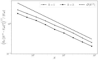
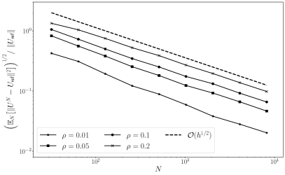
Figure 1. The relative errors $\big{(}\mathbb{E}_{N}\big{[}\|U^{N}-U_{\text{ref}}\|^{2}\big{]}\big{)}^{1/2}/\;\|U_{\text{ref}}\|$ for the nonlinear setting described in Section 6.1. The left plot uses the first randomized strategy and the right plot uses the second strategy. We observe that the errors decay as $\mathcal{O}(h^{1/2})$, in line with Theorem 5.2, irrespective of the choice of $\rho$ or $k$. A smaller $\rho$ or larger $k$ decreases the error, but of course also incurs a higher computational cost.

6.2. A linear example

As a second experiment, we consider a linear version of the previous problem. We use the same parameters as in the previous section, except that we set $p=2$ and $\alpha(t)=0.1$, and that the rotating pulse is now Gaussian rather than a sharp peak. More precisely, the exact solution is given by

$$u(t,x,y)=e^{-100(x-r\cos(2\pi t))^{2}-100(y-r\sin(2\pi t))^{2}}.$$

The resulting errors are shown in Figure 2. Again, we note that the first, uniform, strategy converges as $\mathcal{O}(h^{1/2})$, in line with Theorem 5.2. The second strategy with $\rho=0.01$ performs significantly better and converges as $\mathcal{O}(h)$ until the spatial error starts to dominate. This is essentially the same behaviour as if we would apply backward Euler to the full problem, but the method only updates the approximation on the most relevant sub-domains and is therefore cheaper to evaluate. This improved convergence order is possible due to the extra smoothness present in this linear problem. In the error bound of Theorem 5.2, the first term becomes small due to the used strategy, and because the solution is smooth the remaining terms are of size $h^{3}$ and $h^{2}$, respectively.

Increasing the parameter $\rho$ means that we disregard more of the information from the predictor, and as seen in Figure 2 this causes the convergence order to decrease towards $1/2$. On the other hand, setting $\rho=0$ means that we always choose all the sub-domains and thereby do more computations than if we would simply solve the full problem directly. The parameter $\rho$ is therefore a design parameter, and further research is required on how to choose it optimally for specific problem classes. Regardless of the choice, however, we still have $\mathcal{O}(h^{1/2})$-convergence.

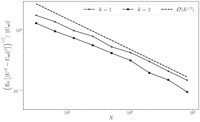
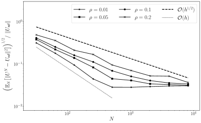
Figure 2. The relative errors $\big{(}\mathbb{E}_{N}\big{[}\|U^{N}-U_{\text{ref}}\|^{2}\big{]}\big{)}^{1/2}/\;\|U_{\text{ref}}\|$ for the linear setting described in Section 6.2. The left plot uses the first randomized strategy and the right plot uses the second strategy. We observe that the errors for the first strategy decay as $\mathcal{O}(h^{1/2})$, similarly to the nonlinear case. For the second strategy, large $\rho$ also leads to convergence of order 1/2, while sufficiently small $\rho$ leads to faster convergence of order $1$. We note that the errors plateau at around $2\cdot 10^{-2}$ because we compare the numerical approximations to the exact solution; this is the size of the spatial error.

Appendix A Auxiliary results

In this appendix, we collect a few useful inequalities and technical results that are needed in the paper.

Lemma A.1 (Grönwall).

Let $(u_{n})_{n\in N}$ and $(b_{n})_{n\in N}$ be two nonnegative sequences that satisfy, for given $a\in[0,\infty)$ and $n\in\mathbb{N}$, that $u_{n}\leq a+\sum_{i=1}^{n}b_{i}u_{i}$. For $b_{n}\in[0,1)$, it then follows that

$$u_{n}\leq\frac{a}{1-b_{n}}\exp\Big{(}\sum_{i=1}^{n-1}\frac{b_{i}}{1-b_{n}}\Big{)}.$$

Lemma A.2 (Scaled Young’s inequality).

For $a,b\in[0,\infty)$, $\varepsilon\in(0,\infty)$, it follows that $ab\leq\varepsilon a^{2}+\frac{1}{4\varepsilon}b^{2}$.

A proof can be found in [12, Appendix B.2 d].

Lemma A.3.

Let Assumptions 1–5 be fulfilled. Let $Q\subseteq V$ be a countable, dense subset of $V$, $V_{\xi}$ and $H$. Let the function $g\colon\Omega\times H\to V^{*}$ be given. Further, for $v\in H$ the mapping $\omega\mapsto\langle g(\omega,v),w\rangle_{V^{*}\times V}$ is measurable for $v\in H$ and $w\in Q$ and for almost every $\omega\in\Omega$ the mapping $v\mapsto\langle g(\omega,v),w\rangle_{V^{*}\times V}$ continuous for every $v,w\in V_{\xi(\omega)}$. For every $\omega\in\Omega$, the function $g$ has a unique root which lies in $V_{\xi(\omega)}$. We denote this root by $r(\omega)\in V_{\xi(\omega)}$, i.e. $g(\omega,r(\omega))=0$. Then the function $r\colon\Omega\to H$ is measurable.

A similar proof can be found in [5, Lemma 2.1.4] and [8, Lemma 4.3]. The main difference in this version is that the function $g$ maps from $\Omega\times H$ instead of $\Omega\times V$ and therefore some small technical alterations have to be considered.

Proof of Lemma A.3.

To prove that $r$ is measurable, we show that $r^{-1}(B)\in\mathcal{F}$ for every open set $B$ in $H$. First, we notice that

$$r^{-1}(B) =\{\omega\in\Omega\colon r(\omega)\in B\}$$

$$=\{\omega\in\Omega\colon\text{ there exists $u\in B$ such that }g(\omega,u)=0\}$$

$$=\{\omega\in\Omega\colon\text{ there exists $u\in B$ such that }\langle g(\omega,u),v\rangle_{V^{*}\times V}=0$$

$$\hskip 199.16928pt\text{ for all }v\in Q,\|v\|_{V}=1\}$$

$$=\bigcap_{v\in Q,\|v\|_{V}=1}\{\omega\in\Omega\colon\text{ there exists $u\in B$ such that }\langle g(\omega,u),v\rangle_{V^{*}\times V}=0\}$$

$$=\bigcap_{v\in Q,\|v\|_{V}=1}\bigcup_{u\in B}\{\omega\in\Omega\colon\langle g(\omega,u),v\rangle_{V^{*}\times V}=0\}.$$

Since $\omega\mapsto\langle g(\omega,v),w\rangle_{V^{*}\times V}$ is measurable for $v\in H$ and $w\in Q$, the set

$$\{\omega\in\Omega\colon\langle g(\omega,u),v\rangle_{V^{*}\times V}=0\}=\big{(}\langle g(\cdot,u),v\rangle_{V^{*}\times V}\big{)}^{-1}(0)$$

is an element of $\mathcal{F}_{\xi}$ for $v\in Q$ and $u\in H$. If the set $B$ only contains a countable amount of elements, it follows directly that $r^{-1}(B)\in\mathcal{F}_{\xi}$.

In the following, it remains to address the cases where $B$ is not countable. For $\varepsilon\in(0,\infty)$ small enough and a fixed $v\in Q$, we introduce the multi-valued mapping

$$r_{\varepsilon}^{v}\colon\Omega\to 2^{H},\quad r_{\varepsilon}^{v}(\omega) =\{u\in H\colon|\langle g(\omega,u),v\rangle_{V^{*}\times V}|<\varepsilon\}.$$

For $B\subseteq H$ open, it follows that

$$\big{(}r_{\varepsilon}^{v}\big{)}^{-1}(B) =\{\omega\in\Omega\colon r_{\varepsilon}^{v}(\omega)\in B\}$$

$$=\{\omega\in\Omega\colon\text{ there exists $u\in B$ such that }|\langle g(\omega,u),v\rangle_{V^{*}\times V}|<\varepsilon\}$$

$$=\bigcup_{u\in B}\{\omega\in\Omega\colon|\langle g(\omega,u),v\rangle_{V^{*}\times V}|<\varepsilon\}.$$

In the following, we will show that

$$\big{(}r_{\varepsilon}^{v}\big{)}^{-1}(B)=\big{(}r_{\varepsilon}^{v}\big{)}^{-1}(B\cap Q).$$

Since $B\cap Q\subseteq B$, it directly follows that $\big{(}r_{\varepsilon}^{v}\big{)}^{-1}(B\cap Q)\subseteq\big{(}r_{\varepsilon}^{v}\big{)}^{-1}(B)$. It remains to verify that $\big{(}r_{\varepsilon}^{v}\big{)}^{-1}(B)\subseteq\big{(}r_{\varepsilon}^{v}\big{)}^{-1}(B\cap Q)$. Let $\omega\in\big{(}r_{\varepsilon}^{v}\big{)}^{-1}(B)$, i.e. there exists $u\in B$ such that

$$u\in r_{\varepsilon}^{v}(\omega)=\{w\in H\colon|\langle g(\omega,w),v\rangle_{V^{*}\times V}|<\varepsilon\}.$$

Since $v\mapsto\langle g(\omega,v),w\rangle_{V^{*}\times V}$ is continuous for every $v,w\in V_{\xi(\omega)}$ and $Q$ is dense in $H$, there exists $u_{Q}\in B\cap Q$ such that $|\langle g(\omega,u_{Q}),v\rangle_{V^{*}\times V}|<\varepsilon$. Thus, $u_{Q}\in r_{\varepsilon}^{v}(\omega)$ and in particular $\omega\in\big{(}r_{\varepsilon}^{v}\big{)}^{-1}(B\cap Q)$. This shows altogether that $\big{(}r_{\varepsilon}^{v}\big{)}^{-1}(B)=\big{(}r_{\varepsilon}^{v}\big{)}^{-1}(B\cap Q)$.

We can now finish the proof as

$$r^{-1}(B)=\bigcap_{v\in Q,\|v\|_{V}=1}\bigcap_{i\in\mathbb{N}}\big{(}r_{\frac{1}{i}}^{v}\big{)}^{-1}(B)=\bigcap_{v\in Q,\|v\|_{V}=1}\bigcap_{i\in\mathbb{N}}\big{(}r_{\frac{1}{i}}^{v}\big{)}^{-1}(B\cap Q)\in\mathcal{F}_{\xi}$$

is fulfilled. ∎

Lemma A.4.

Let Assumptions 1–5 be fulfilled. Further, let $f_{\xi_{n}}$ be an element of $C([0,T];V_{\xi_{n}}^{*})$ almost surely for every $n\in\{1.\dots.N\}$. For $u^{\prime}\in C^{\gamma}([0,T];H)$, $\gamma\in(0,1]$, and a maximal step size $h=\max_{i\in\{1,\dots,N\}}h_{i}$, it the follows that

$$\sum_{i=1}^{N}h_{i}\mathbb{E}_{\xi_{i}}\Big{[}\Big{\|}f_{\xi_{i}}(t_{i})-A_{\xi_{i}}(t_{i})u(t_{i})-\frac{1}{h_{i}}\int_{t_{i-1}}^{t_{i}}\big{(}f(t)-A(t)u(t)\big{)}\,\mathrm{d}t\Big{\|}_{H}^{2}\Big{]}$$

$$\leq 2\sum_{i=1}^{N}h_{i}\mathbb{E}_{\xi_{i}}\big{[}\big{\|}f_{\xi_{i}}(t_{i})-A_{\xi_{i}}(t_{i})u(t_{i})-(f(t_{i})-A(t_{i})u(t_{i}))\big{\|}_{H}^{2}\big{]}$$

$$\quad+2h^{2\gamma}|u^{\prime}|_{C^{\gamma}([0,T];H)}^{2}T$$

and

$$\sum_{i=1}^{N}h_{i}\Big{\|}\mathbb{E}_{\xi_{i}}\Big{[}f_{\xi_{i}}(t_{i})-A_{\xi_{i}}(t_{i})u(t_{i})-\frac{1}{h_{i}}\int_{t_{i-1}}^{t_{i}}\big{(}f(t)-A(t)u(t)\big{)}\,\mathrm{d}t\Big{]}\Big{\|}_{H}^{2}$$

$$\leq h^{2\gamma}|u^{\prime}|_{C^{\gamma}([0,T];H)}^{2}T,$$

where $|u^{\prime}|_{C^{\gamma}([0,T];H)}$ is the Hölder semi-norm with values in $H$ of the function $u^{\prime}$.

Proof.

To prove the first bound, we find that

$$\sum_{i=1}^{N}h_{i}\mathbb{E}_{\xi_{i}}\Big{[}\Big{\|}f_{\xi_{i}}(t_{i})-A_{\xi_{i}}(t_{i})u(t_{i})-\frac{1}{h_{i}}\int_{t_{i-1}}^{t_{i}}\big{(}f(t)-A(t)u(t)\big{)}\,\mathrm{d}t\Big{\|}_{H}^{2}\Big{]}$$

$$\leq 2\sum_{i=1}^{N}h_{i}\mathbb{E}_{i}\big{[}\big{\|}f_{\xi_{i}}(t_{i})-A_{\xi_{i}}(t_{i})u(t_{i})-(f(t_{i})-A(t_{i})u(t_{i}))\big{\|}_{H}^{2}\big{]}$$

$$\quad+2\sum_{i=1}^{N}h_{i}\mathbb{E}_{i}\Big{[}\Big{\|}\frac{1}{h_{i}}\int_{t_{i-1}}^{t_{i}}\big{(}f(t_{i})-A(t_{i})u(t_{i})-(f(t)-A(t)u(t))\big{)}\,\mathrm{d}t\Big{\|}_{H}^{2}\Big{]}$$

$$\leq 2\sum_{i=1}^{N}h_{i}\mathbb{E}_{i}\big{[}\big{\|}f_{\xi_{i}}(t_{i})-A_{\xi_{i}}(t_{i})u(t_{i})-(f(t_{i})-A(t_{i})u(t_{i}))\big{\|}_{H}^{2}\big{]}$$

$$\quad+2\sum_{i=1}^{N}\frac{1}{h_{i}}\Big{\|}\int_{t_{i-1}}^{t_{i}}(u^{\prime}(t_{i})-u^{\prime}(t))\,\mathrm{d}t\Big{\|}_{H}^{2}.$$

To further bound the last row, we apply Hölder’s inequality and the regularity condition $u^{\prime}\in C^{\gamma}([0,T];H)$. We then find that

$$2\sum_{i=1}^{N}\frac{1}{h_{i}}\Big{\|}\int_{t_{i-1}}^{t_{i}}(u^{\prime}(t_{i})-u^{\prime}(t))\,\mathrm{d}t\Big{\|}_{H}^{2} \leq 2\sum_{i=1}^{N}\int_{t_{i-1}}^{t_{i}}\|u^{\prime}(t_{i})-u^{\prime}(t)\|_{H}^{2}\,\mathrm{d}t$$

$$\leq 2h^{2\gamma}|u^{\prime}|_{C^{\gamma}([0,T];H)}^{2}T.$$

It remains to prove the second estimate of the lemma. Recall that $\mathbb{E}_{\xi_{i}}\big{[}f_{\xi_{i}}(t_{i})\big{]}=f(t_{i})$ and $\mathbb{E}_{\xi_{i}}\big{[}A_{\xi_{i}}(t_{i})u(t_{i})\big{]}=A(t_{i})u(t_{i})$ is fulfilled by Assumption 5. Using these equalities, it follows that

$$\sum_{i=1}^{N}h_{i}\Big{\|}\mathbb{E}_{\xi_{i}}\Big{[}f_{\xi_{i}}(t_{i})-A_{\xi_{i}}(t_{i})u(t_{i})-\frac{1}{h_{i}}\int_{t_{i-1}}^{t_{i}}\big{(}f(t)-A(t)u(t)\big{)}\,\mathrm{d}t\Big{]}\Big{\|}_{H}^{2}$$

$$=\sum_{i=1}^{N}h_{i}\Big{\|}f(t_{i})-A(t_{i})u(t_{i})-\frac{1}{h_{i}}\int_{t_{i-1}}^{t_{i}}(f(t)-A(t)u(t))\,\mathrm{d}t\Big{\|}_{H}^{2}$$

$$\leq\sum_{i=1}^{N}\int_{t_{i-1}}^{t_{i}}\|u^{\prime}(t_{i})-u^{\prime}(t)\|_{H}^{2}\,\mathrm{d}t\leq h^{2\gamma}|u^{\prime}|_{C^{\gamma}([0,T];H)}^{2}T.$$

∎

References

- [1] G. Aronsson, L. C. Evans, and Y. Wu. Fast/slow diffusion and growing sandpiles. J. Differential Equations, 131(2):304–335, 1996.
- [2] T. Bochacik, M. Goćwin, P. M. Morkisz, and P. Przybyłowicz. Randomized Runge-Kutta method—stability and convergence under inexact information. J. Complexity, 65:Paper No. 101554, 21, 2021.
- [3] L. Bottou, F. E. Curtis, and J. Nocedal. Optimization methods for large-scale machine learning. SIAM Rev., 60(2):223–311, 2018.
- [4] T. Daun. On the randomized solution of initial value problems. J. Complexity, 27(3-4):300–311, 2011.
- [5] M. Eisenmann. Methods for the Temporal Approximation of Nonlinear, Nonautonomous Evolution Equations. PhD thesis, TU Berlin, 2019.
- [6] M. Eisenmann and E. Hansen. Convergence analysis of domain decomposition based time integrators for degenerate parabolic equations. Numer. Math., 140(4):913–938, 2018.
- [7] M. Eisenmann and E. Hansen. A variational approach to the sum splitting scheme. IMA J. Numer. Anal., 42(1):923–950, 2022.
- [8] M. Eisenmann, M. Kovács, R. Kruse, and S. Larsson. On a randomized backward Euler method for nonlinear evolution equations with time-irregular coefficients. Found. Comput. Math., 19(6):1387–1430, 2019.
- [9] M. Eisenmann, T. Stillfjord, and M. Williamson. Sub-linear convergence of a stochastic proximal iteration method in Hilbert space. Comput. Optim. Appl., 83(1):181–210, 2022.
- [10] E. Emmrich. Two-step BDF time discretisation of nonlinear evolution problems governed by monotone operators with strongly continuous perturbations. Comput. Methods Appl. Math., 9(1):37–62, 2009.
- [11] E. Emmrich and M. Thalhammer. Stiffly accurate Runge-Kutta methods for nonlinear evolution problems governed by a monotone operator. Math. Comp., 79(270):785–806, 2010.
- [12] L. C. Evans. Partial Differential Equations. American Mathematical Society, Providence, RI, 1998.
- [13] E. Hansen and E. Henningsson. Additive domain decomposition operator splittings—convergence analyses in a dissipative framework. IMA J. Numer. Anal., 37(3):1496–1519, 2017.
- [14] E. Hansen and A. Ostermann. Dimension splitting for quasilinear parabolic equations. IMA J. Numer. Anal., 30(3):857–869, 2010.
- [15] E. Hansen and T. Stillfjord. Convergence of the implicit-explicit Euler scheme applied to perturbed dissipative evolution equations. Math. Comp., 82(284):1975–1985, 2013.
- [16] W. Hundsdorfer and J. Verwer. Numerical Solution of Time-Dependent Advection-Diffusion-Reaction Equations. Springer-Verlag, Berlin, 2003.
- [17] E. R. Jakobsen and K. H. Karlsen. Convergence rates for semi-discrete splitting approximations for degenerate parabolic equations with source terms. BIT, 45(1):37–67, 2005.
- [18] A. Jentzen and A. Neuenkirch. A random Euler scheme for Carathéodory differential equations. J. Comput. Appl. Math., 224(1):346–359, 2009.
- [19] S. Jin, L. Li, and J.-G. Liu. Random batch methods (RBM) for interacting particle systems. J. Comput. Phys., 400:108877, 30, 2020.
- [20] S. Jin, L. Li, and J.-G. Liu. Convergence of the random batch method for interacting particles with disparate species and weights. SIAM J. Numer. Anal., 59(2):746–768, 2021.
- [21] S. Kamin and J. L. Vázquez. Fundamental solutions and asymptotic behaviour for the -Laplacian equation. Rev. Mat. Iberoamericana, 4(2):339–354, 1988.
- [22] R. Kruse and Y. Wu. Error analysis of randomized Runge-Kutta methods for differential equations with time-irregular coefficients. Comput. Methods Appl. Math., 17(3):479–498, 2017.
- [23] R. Kruse and Y. Wu. A randomized and fully discrete Galerkin finite element method for semilinear stochastic evolution equations. Math. Comp., 2019.
- [24] R. Kruse and Y. Wu. A randomized Milstein method for stochastic differential equations with non-differentiable drift coefficients. Discrete Contin. Dyn. Syst. Ser. B, 24(8):3475–3502, 2019.
- [25] A. Kufner. Weighted Sobolev Spaces. BSB B. G. Teubner Verlagsgesellschaft, Leipzig, 1980.
- [26] A. Kuijper. -Laplacian driven image processing. In 2007 IEEE International Conference on Image Processing, volume 5, pages V – 257–V – 260, 2007.
- [27] G. Leoni. A First Course in Sobolev Spaces. American Mathematical Society, Providence, RI, 2009.
- [28] L. Li, Z. Xu, and Y. Zhao. A random-batch Monte Carlo method for many-body systems with singular kernels. SIAM J. Sci. Comput., 42(3):A1486–A1509, 2020.
- [29] P.-L. Lions and B. Mercier. Splitting algorithms for the sum of two nonlinear operators. SIAM J. Numer. Anal., 16(6):964–979, 1979.
- [30] T. Mathew. Domain Decomposition Methods for the Numerical Solution of Partial Differential Equations. Springer-Verlag, Berlin, 2008.
- [31] T. P. Mathew, P. L. Polyakov, G. Russo, and J. Wang. Domain decomposition operator splittings for the solution of parabolic equations. SIAM J. Sci. Comput., 19(3):912–932, 1998.
- [32] H. Robbins and S. Monro. A stochastic approximation method. Ann. Math. Statistics, 22:400–407, 1951.
- [33] T. Roubíček. Nonlinear Partial Differential Equations with Applications. Birkhäuser, Basel, second edition, 2013.
- [34] G. Stengle. Numerical methods for systems with measurable coefficients. Appl. Math. Lett., 3(4):25–29, 1990.
- [35] G. Stengle. Error analysis of a randomized numerical method. Numer. Math., 70(1):119–128, 1995.
- [36] D. Stone, S. Geiger, and G. J. Lord. Asynchronous discrete event schemes for PDEs. J. Comput. Phys., 342:161–176, 2017.
- [37] J. L. Vázquez. The Porous Medium Equation. Oxford Mathematical Monographs. The Clarendon Press, Oxford University Press, Oxford, 2007. Mathematical theory.
- [38] D. W. M. Veldman and E. Zuazua. A framework for randomized time-splitting in linear-quadratic optimal control. Numer. Math., 151(2):495–549, 2022.