DeepPerform: An Efficient Approach for Performance Testing of Resource-Constrained Neural Networks

Abstract.

Today, an increasing number of Adaptive Deep Neural Networks (AdNNs) are being used on resource-constrained embedded devices. We observe that, similar to traditional software, redundant computation exists in AdNNs, resulting in considerable performance degradation. The performance degradation is dependent on the input and is referred to as input-dependent performance bottlenecks (IDPBs). To ensure an AdNN satisfies the performance requirements of resource-constrained applications, it is essential to conduct performance testing to detect IDPBs in the AdNN. Existing neural network testing methods are primarily concerned with correctness testing, which does not involve performance testing. To fill this gap, we propose DeepPerform, a scalable approach to generate test samples to detect the IDPBs in AdNNs. We first demonstrate how the problem of generating performance test samples detecting IDPBs can be formulated as an optimization problem. Following that, we demonstrate how DeepPerform efficiently handles the optimization problem by learning and estimating the distribution of AdNNs’ computational consumption. We evaluate DeepPerform on three widely used datasets against five popular AdNN models. The results show that DeepPerform generates test samples that cause more severe performance degradation (FLOPs: increase up to 552%). Furthermore, DeepPerform is substantially more efficient than the baseline methods in generating test inputs (runtime overhead: only 6–10 milliseconds).

1. Introduction

Deep Neural Networks (DNNs) have shown potential in many applications, such as image classification, image segmentation, and object detection (Chan et al., 2016; Vaswani et al., 2017; Huang et al., 2018). However, the power of using DNNs comes at substantial computational costs (Najibi et al., 2019; Veit and Belongie, 2018; Wu et al., 2019; Hua et al., 2019; Liu and Deng, 2018). The costs, especially the inference-time cost, can be a concern for deploying DNNs on resource-constrained embedded devices such as mobile phones and IoT devices. To enable deploying DNNs on resource-constrained devices, researchers propose a series of Adaptive Neural Networks (AdNNs) (Wan et al., 2020; Bateni and Liu, 2018; Jiang et al., 2021; Wang et al., 2021; Davis and Arel, 2014; Gao et al., 2018). AdNNs selectively activate partial computation units (e.g., convolution layer, fully connected layer) for different inputs rather than whole units for computation. The partial unit selection mechanism enables AdNNs to achieve real-time prediction on resource-constrained devices.

Similar to the traditional systems (Xiao et al., 2013), performance bottlenecks also exist in AdNNs. Among the performance bottlenecks, some of them can be detected only when given specific input values. Hence, these problems are referred to as input-dependent performance bottlenecks (IDPBs). Some IDPBs will cause severe performance degradation and result in catastrophic consequences. For example, consider an AdNN deployed on a drone for obstacle detection. If AdNNs’ energy consumption increases five times suddenly for specific inputs, it will make the drone out of battery in the middle of a trip. Because of these reasons, conducting performance testing to find IDPB is a crucial step before AdNNs’ deployment process.

However, to the best of our knowledge, most of the existing work for testing neural networks are mainly focusing on correctness testing, which can not be applied to performance testing. The main difference between correctness testing and performance testing is that correctness testing aims to detect models’ incorrect classifications; while the performance testing is to find IDPBs that trigger performance degradation. Because incorrect classifications may not lead to performance degradation, existing correctness testing methods can not be applied for performance testing. To fill this gap and accelerate the process of deploying neural networks on resource-constrained devices, there is a strong need for an automated performance testing framework to find IDPBs.

We identify two main challenges in designing such a performance testing framework. First, traditional performance metrics (e.g., latency, energy consumption) are hardware-dependent metrics. Measuring these hardware-dependent metrics requires repeated experiments because of the system noises. Thus, directly applying these hardware-dependent metrics as guidelines to generate test samples would be inefficient. Second, AdNNs’ performance adjustment strategy is learned from datasets rather than conforming to logic specifications (such as relations between model inputs and outputs). Without a logical relation between AdNNs’ inputs and AdNNs’ performance, it is challenging to search for inputs that can trigger performance degradation in AdNNs.

To address the above challenges, we propose DeepPerform, which enables efficient performance testing for AdNNs by generating test samples that trigger IDPBs of AdNNs (DeepPerform focuses on the performance testing of latency degradation and energy consumption degradation as these two metrics are critical for performance testing (Bateni and Liu, 2020; Wan et al., 2020)). To address the first challenge, we first conduct a preliminary study (§3) to illustrate the relationship between computational complexity (FLOPs) and hardware-dependent performance metrics (latency, energy consumption). We then transfer the problem of degrading system performance into increasing AdNNs’ computational complexity (Eq.(3)). To address the second challenge, we apply the a paradigm similar to Generative Adversarial Networks (GANs) to design DeepPerform. In the training process, DeepPerform learns and approximates the distribution of the samples that require more computational complexity. After DeepPerform is well trained, DeepPerform generates test samples that activate more redundant computational units in AdNNs. In addition, because DeepPerform does not require backward propagation during the test sample generation phase, DeepPerform generates test samples much more efficiently, thus more scalable for comprehensive testing on large models and datasets.

To evaluate DeepPerform, we select five widely-used model-dataset pairs as experimental subjects and explore following four perspectives: effectiveness, efficiency, coverage, and sensitivity. First, to evaluate the effectiveness of the performance degradation caused by test samples generated by DeepPerform, we measure the increase in computational complexity (FLOPs) and resource consumption (latency, energy) caused by the inputs generated by DeepPerform. For measuring efficiency, we evaluate the online time-overheads and total time-overheads of DeepPerform in generating different scale samples for different scale experimental subjects. For coverage evaluation, we measure the computational units covered by the test inputs generated by DeepPerform. For sensitivity measurement, we measure how DeepPerform’s effectiveness is dependent on the ADNNs’ configurations and hardware platforms. The experimental results show that DeepPerform generated inputs increase AdNNs’ computational FLOPs up to 552%, with 6-10 milliseconds overheads for generating one test sample. We summarize our contribution as follows:

• Approach. We propose a learning-based approach , namely DeepPerform, to learn the distribution to generate the test samples for performance testing. Our novel design enables generating test samples more efficiently, thus enable scalable performance testing.

• Evaluation. We evaluate DeepPerform on five AdNN models and three datasets. The evaluation results suggest that DeepPerform finds more severe diverse performance bugs while covering more AdNNs’ behaviors, with only 6-10 milliseconds of online overheads for generating test inputs.

• Application. We demonstrate that developers could benefit from DeepPerform. Specifically, developers can use the test samples generated by DeepPerform to train a detector to filter out the inputs requiring high abnormal computational resources (§6).

2. Background

2.1. AdNNs’ Working Mechanisms

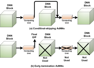
Figure 1. Working mechanism of AdNNs

The main objective of AdNNs (Wan et al., 2020; Teerapittayanon et al., 2016; Bolukbasi et al., 2017; Kaya et al., 2019; Wang et al., 2018; Davis and Arel, 2014; Gao et al., 2018; Shazeer et al., 2017; Lin et al., 2017; Nan and Saligrama, 2017) is to balance performance and accuracy. As shown in Fig. 2, AdNNs will allocate more computational resources to inputs with more complex semantics. AdNNs use intermediate outputs to deactivate specific components of neural networks, thus reducing computing resource consumption. According to the working mechanism, AdNNs can be divided mainly into two types: Conditional-skipping AdNNs and Early-termination AdNNs, as shown in Fig. 1. Conditional-skipping AdNNs skip specific layers/blocks if the intermediate outputs provided by specified computing units match predefined criteria. (in the case of ResNet). The working mechanism of the conditional-skipping AdNN can be formulated as:

(1) $$\begin{cases}In_{i+1}=Out_{i},\quad\text{if}\ B_{i}(x)\geq\tau_{i}\\ Out_{i+1}=Out_{i},\quad\text{otherwise}\end{cases}$$

where $x$ is the input, $In_{i}$ represents the input of $i^{th}$ layer, $Out_{i}$ represents the output of $i^{th}$ layer, $B_{i}$ represents the specified computing unit output of $i^{th}$ layer and $\tau_{i}$ is the configurable threshold that decides AdNNs’ performance-accuracy trade-off mode. Early-termination AdNNs terminate computation early if the intermediate outputs satisfy a particular criteria. The working mechanism of early-termination AdNNs can be formulated as,

(2) $$\begin{cases}Exit_{NN}(x)=Exit_{i}(x),\quad\text{if}\ B_{i}(x)\geq\tau_{i}\\ In_{i+1}(x)=Out_{i}(x),\quad\quad\text{otherwise}\end{cases}$$

2.2. Redundant Computation

In a software program, if an operation is not required but performed, we term the operation as redundant operation. For Adaptive Neural Networks, if a component is activated without affecting AdNNs’ final predictions, we define the computation as a redundant computation. AdNNs are created based on the philosophy that all the inputs should not require all DNN components for inference. For example, we can refer to the images in Fig. 2. The left box shows the AdNNs’ design philosophy. That is, AdNNs consume more energy for detecting images with further complexity. However, when the third image in the left box is perturbed with minimal perturbations and becomes the rightmost one, AdNNs’ inference energy consumption will increase significantly (from $30j$ to $68j$). We refer to such additional computation as redundant computation or performance degradation.

2.3. Performance & Computational Complexity

In this section, we describe the relationship between hardware-dependent performance metrics and DNN computational complexity. Although many metrics can reflect DNN performance, we chose latency and energy consumption as hardware-dependent performance metrics because of their critical nature for real-time embedded systems (Bateni and Liu, 2020; Wan et al., 2020). Measuring hardware-dependent performance metrics (e.g., latency, energy consumption) usually requires many repeated experiments, which is costly. Hence, existing work (Wang et al., 2018; Davis and Arel, 2014; Gao et al., 2018; Shazeer et al., 2017; Lin et al., 2017; Nan and Saligrama, 2017) proposes to apply floating point operations (FLOPs) to represent DNN computational complexity. However, a recent study (Tang et al., 2021) demonstrates that simply lowering DNN computational complexity (FLOPs) does not always improve DNN runtime performance. This is because modern hardware platforms usually apply parallelism to handle DNN floating-point operations (FLOPs). Parallelism can accelerate computation within layers, while each DNN layer is computed sequentially. Thus, For two DNNs with the same total FLOPs, different FLOPs allocating strategies will result in different parallelism utilization and different DNN model performance. However, for AdNNs, each layer/block usually has a similar structure and FLOPs (Wang et al., 2018; Davis and Arel, 2014; Gao et al., 2018; Najibi et al., 2019). Thus the parallelism utilization is similar for each block. Because parallelism can not accelerate computation between blocks, increasing the number of computational blocks/layers will degrade AdNNs’ performance. To further understand the relation between AdNNs’ FLOPs and AdNNs’ model performance, we conduct a study in §3.

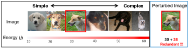
Figure 2. Left Box shows that AdNNs allocate different computational resources for images with different semantic complexity; rights box shows that perturbed image could trigger redundant computation and cause energy surge.

3. Preliminary Study

Table 1. Experiential subject and model performance

Subject		FLOPs			CPU (Quad-Core ARM® Cortex®-A57 MPCore)						GPU (NVIDIA Pascal™ GPU architecture with 256 cores)
					Latency			Energy			Latency			Energy
Dataset	Model	Min	Avg	Max	Min	Avg	Max	Min	Avg	Max	Min	Avg	Max	Min	Avg	Max
CIFAR10 (C10)	SkipNet (SN)	195.44	248.62	336.99	0.44	0.51	0.63	65.76	76.60	316.44	0.74	0.94	1.39	168.07	245.62	439.38
	BlockDrop (BD)	72.56	180.51	228.27	0.11	0.23	0.37	15.89	34.17	161.12	0.13	0.33	0.71	29.60	73.27	282.59
CIFAR100 (C100)	DeepShallow (DS)	38.68	110.47	252.22	0.04	0.11	0.25	3.47	15.32	37.81	0.09	0.37	1.08	12.63	75.49	441.60
	RaNet (RN)	31.50	41.79	188.68	0.07	0.21	2.96	8.21	27.99	448.96	0.10	0.36	5.81	15.87	60.22	997.73
SVHN	DeepShallow (DS)	38.74	161.40	252.95	0.04	0.16	0.27	3.99	23.35	91.28	0.03	0.37	0.82	4.16	78.66	180.39

3.1. Study Approach

Our intuition is to explore the worst computational complexity of an algorithm or model. For AdNNs, the basic computation are the floating-point operations (FLOPs). Thus, we made an assumption that the FLOPs count of an AdNN is a hardware-independent metric to approximate AdNN performance. To validate such an assumption, we conduct an empirical study. Specifically, we compute the Pearson Product-moment Correlation Co-efficient (PCCs) (Rice, 2006) between AdNN FLOPs against AdNN latency and energy consumption. PCCs are widely used in statistical methods to measure the linear correlation between two variables. PCCs are normalized covariance measurements, ranging from -1 to 1. Higher PCCs indicate that the two variables are more positively related. If the PCCs between FLOPs against system latency and system energy consumption are both high, then we validate our assumption.

3.2. Study Model & Dataset

We select subjects (e.g., model,dataset) following policies below.

• The selected subjects are publicly available.

• The selected subjects are widely used in existing work.

• The selected dataset and models should be diverse from different perspectives. e.g.,, the selected models should include both early-termination and conditional-skipping AdNNs.

We select five popular model-dataset combinations used for image classification tasks as our experimental subjects. The dataset and the corresponding model are listed in Table 1. We explain the selected datasets and corresponding models below.

Datasets. CIFAR-10 (Krizhevsky et al., 2009) is a database for object recognition. There is a total of ten object classes for this dataset, and the image size of the image in CIFAR-10 is $32\times 32$. CIFAR-10 contains 50,000 training images and 10,000 testing images. CIFAR-100 (Krizhevsky et al., 2009) is similar to CIFAR-10 (Krizhevsky et al., 2009) but with 100 classes. It also contains 50,000 training images and 10,000 testing images. SVHN (Netzer et al., 2011) is a real-world image dataset obtained from house numbers in Google Street View images. There are 73257 training images and 26032 testing images in SVHN.

Models. For CIFAR-10 dataset, we use SkipNet (Wang et al., 2018) and BlockDrop (Wu et al., 2018) models. SkipNet applies reinforcement learning to train DNNs to skip unnecessary blocks, and BlockDrop trains a policy network to activate partial blocks to save computation costs. We download trained SkipNet and BlockDrop from the authors’ websites. For CIFAR-100 dataset, we use RaNet (Yang et al., 2020) and DeepShallow (Kaya et al., 2019) models for evaluation. DeepShallow adaptive scales DNN depth, while RaNet scales both input resolution and DNN depth to balance accuracy and performance. For SVHN dataset, DeepShallow (Kaya et al., 2019) is used for evaluation. For RaNet (Yang et al., 2020) and DeepShallow (Kaya et al., 2019) architecture, the author does not release the trained model weights but open-source their training codes. Therefore, we follow the authors’ instructions to train the model weights.

3.3. Study Process

We begin by evaluating each model’s computational complexity on the original hold-out test dataset. After that, we deploy the AdNN model on an Nvidia TX2 (Nvidia, [n. d.]) and measure latency and energy usage. Through Table 1, we present the FLOPs, latency, and energy consumption of each AdNN. We observe that the model would cost a different number of FLOPs for different test samples, and the variance between each test sample could be significant. For instance, for dataset CIFAR-100 and model RaNet, the minimum FLOPs are 31.5M, while the maximum FLOPs are 188.68M.

3.4. Study Results

Table 2. PCCs between FLOPs against latency and energy

Hardware	Metric	SN_C10	RN_C100	BD_C10	DS_C100	DS_SVHN
CPU	Latency	0.68	0.67	0.93	0.99	0.95
	Energy	0.65	0.64	0.93	0.98	0.95
GPU	Latency	0.48	0.56	0.91	0.99	0.97
	Energy	0.53	0.64	0.91	0.99	0.97

From the PCCs results in Table 2, we have the following observations: (i) The PCCs are more than 0.48 for all subjects. The results imply that FLOPs are positively related to latency and energy consumption in AdNNs (Rice, 2006). Especially for DS_C100, the PCC achieves 0.99, which indicates the strong linear relationship between FLOPs and runtime performance. (ii) The PCCs for the same subject on different hardware devices are remarkably similar (e.g.,, with an average difference of 0.04). According to the findings, the PCCs between FLOPs and latency/energy consumption are hardware independent. The statistical observations of PCCs confirm our assumption; that is, the FLOPs of AdNN handling an input is a hardware-independent metric that can approximate AdNN performance on multiple hardware platforms.

3.5. Motivating Example

Table 3. System availability under performance degradation

Subject	Original	Perturbed	Ratio
SN_C10	10,000	6,332	0.6332
BD_C10	10,000	4,539	0.4539
RN_C100	10,000	5,232	0.5232
DS_C100	10,000	3,576	0.3576
DS_SVHN	10,000	4,145	0.4145

To further understand the necessity of conducting performance testing for AdNNs, we use one real-world example to show the harmful consequences of performance degradation. In particular, we use TorchMobile to deploy each AdNN model on Samsung Galaxy S9+, an Android device with 6GB RAM and 3500mAh battery capacity. We randomly select inputs from the original test dataset of each subject (i.e., Table 1) as seed inputs and perturb the selected seed inputs with random perturbation. Next, we conduct two experiments (one on the selected seed inputs and another one on the perturbed one) on the phone with the same battery. Specifically, we feed both datasets into AdNN for object classification and record the number of inputs successfully inferred before the battery runs out (We set the initial battery as the battery that can infer 10,000 inputs from the original dataset). The results are shown in Table 3, where the column “original” and “perturbed” show the number of inputs successfully inferred, and the column “ratio” shows the corresponding system availability ratio (i.e., the system can successfully complete the percentage of the assigned tasks under performance degradation). Such experimental results highlight the importance of AdNN performance testing before deployment. Otherwise, AdNNs’ performance degradation will endanger the deployed system’s availability.

4. Approach

In this section, we introduce the detail design of DeepPerform.

4.1. Performance Test Samples for AdNNs

Following existing work (Haque et al., 2020; Lemieux et al., 2018, 2018), we define performance test samples as the inputs that require redundant computation and cause performance degradation (e.g., higher energy consumption). Because our work focus on testing AdNNs, we begin by introducing redundant computation in AdNNs. Like traditional software, existing work (Kaya et al., 2019; Haque et al., 2020) has shown redundant computation also exist in AdNNs. Formally, let $g_{f}(\cdot)$ denotes the function that measures the computational complexity of neural network $f(\cdot)$, and $T_{I}(\cdot)$ denotes a semantic-equivalent transformation in the input domain. As the example in Fig. 2, $T_{I}(\cdot)$ could be changing some unnoticeable pixels in the input images. If $g_{f}(T_{I}(x_{i}))>g_{f}(x_{i})$ and $f(x_{i})$ is correctly computed, then there exist redundant computation in the model $f(\cdot)$ handling $T_{I}(x_{i})$. In this paper, we consider unnoticeable perturbations as our transformations $T_{I}(\cdot)$, the same as the existing work (Carlini and Wagner, 2017; Jia and Liang, 2017; Haque et al., 2020). Finally, we formulate our objective to generate performance test samples as searching such unnoticeable input transformation $T_{I}(\cdot)$, as shown in Eq.(3).

(3) $$\begin{split}&\qquad g(T_{I}(x))>>g(x)\\ &T_{I}(x)=\{x+\delta(x)|\quad||\delta(x)||_{p}\leq\epsilon\}\end{split}$$

4.2. DeepPerform Framework

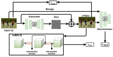
Figure 3. Design overview of DeepPerform

Fig. 3 illustrates the overall architecture of DeepPerform, which is based on the paradigm of Generative Adversarial Networks (GANs). GANs mainly consist of a generator $\mathcal{G}(\cdot)$ and a discriminator $\mathcal{D}(\cdot)$. The input $x$ of the generator $\mathcal{G}(\cdot)$ is a seed input and the output $\mathcal{G}(x)$ is a minimal perturbation (i.e., $\delta(x)$ in Eq.(3)). After applying the generated perturbation to the seed input, the test sample $T_{I}(x)=x+\mathcal{G}(x)$ is sent to the discriminator. The discriminator $\mathcal{D}(\cdot)$ is designed to distinguish the generated test samples $x+\mathcal{G}(x)$ and the original samples $x$. After training, the generator would generate more unnoticeable perturbation, correspondingly, the discriminator would also be more accurate in distinguishing original samples and generated samples. After being well trained, the discriminator and the generator would reach a Nash Equilibrium, which implies the generated test samples are challenging to be distinguished from the original samples.

(4) $$\mathcal{L}_{GAN}=\mathbb{E}_{x}log\mathcal{D}(x)+\mathbb{E}_{x}log[1-\mathcal{D}(x+\mathcal{G}(x))]$$

The loss function of the Generative Adversarial Networks (GANs) can be formulated as Equation 4. In Equation 4, the discriminator $\mathcal{D}$ tries to distinguish the generated samples $\mathcal{G}(x)+x$ and the original sample $x$, so as to encourage the samples generated by $\mathcal{G}$ close to the distribution of the original sample.

However, the perturbation generated by $\mathcal{G}$ may not be able to trigger performance degradation. To fulfil that purpose, we add target AdNN $f(\cdot)$ into the DeepPerform architecture. While training $\mathcal{G}(\cdot)$, the generated input is fed to AdNN to create an objective function that will help increase the AdNNs’ FLOPs consumption. To generate perturbation that triggers performance degradation in AdNNs, we incorporate two more loss functions other than $\mathcal{L}_{GAN}$ for training $\mathcal{G}(\cdot)$. As shown in Eq.(3), to increase the redundant computation, the first step is to model the function $g_{f}(\cdot)$. According to our statistical results in §3, FLOPs could be applied as a hardware-independent metric to approximate AdNNs system performance. Then we model $g_{f}(\cdot)$ as Eq.(5).

(5) $$g_{f}(x)=\sum_{i=1}^{N}W_{i}\times\mathbb{I}(B_{i}(x)>\tau_{i})$$

Where $W_{i}$ is the FLOPs in the $i^{th}$ block, $B_{i}(x)$ is the probability that the $i^{th}$ block is activated, $\mathbb{I}(\cdot)$ is the indicator function, and $\tau_{i}$ is the pre-set threshold based on available computational resources.

(6) $$\mathcal{L}_{adv}=\ell(g_{f}(x),\;\sum_{i=1}^{N}W_{i})$$

To enforce $\mathcal{G}$ could generate perturbation that trigger IDPB, we define our performance degradation objective function as Equation 6. Where $\ell$ is the Mean Squared Error. Recall $\sum_{i=1}^{N}W_{i}$ is the status that all blocks are activated, then $\mathcal{L}_{adv}$ would encourage the perturbed input to activate all blocks of the model, thus triggering IDPBs.

(7) $$\mathcal{L}_{per}=\mathbb{E}_{x}||\mathcal{G}(x)||_{p}$$

To bound the magnitude of the perturbation, we follow the existing work (Carlini and Wagner, 2017) to add a loss of the $L_{p}$ norm of the semantic-equivalent perturbation. Finally, our full objective can be denoted as

(8) $$\mathcal{L}=\mathcal{L}_{GAN}+\alpha\mathcal{L}_{adv}+\beta\mathcal{L}_{per}$$

Where $\alpha$ and $\beta$ are two hyper-parameters that balance the importance of each objective. Notice that the goal of the correctness-based testing methods’ objective function is to maximize the errors while our objective function is to maximize the computational complexity. Thus, our objective function in Eq.(8) can not be replaced by the objective function proposed in correctness-based testing (Carlini and Wagner, 2017; Pei et al., 2017; Tian et al., 2018).

4.3. Architecture Details

In this section, we introduce the detailed architecture of the generator and the discriminator. Our generator $\mathcal{G}$ adapts the structure of encoder-decoder, and the architecture of the discriminator is a convolutional neural network. The architectures of the generator and the discriminator are displayed in Fig. 4.

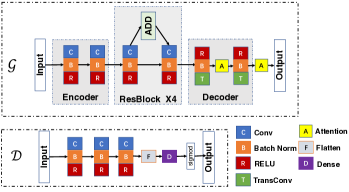
Figure 4. Architecture of the generator and discriminator

Generator. As shown in Fig. 4, there are three main components in the generator, that is, the Encoder, the ResBlocks, and the Decoder. The Encoder repeats the convolutional blocks twice, a convolutional block includes a convolutional layer, a batch normalization layer, and a RELU activation layer. After the encoding process, the input would be smaller in size but with deep channels. The ResBlock stacks four residual blocks (Han et al., 2015), which is widely used to avoid the gradient vanishing problem. The Decoder is the reverse process of the Encoder, the transpose convolutional layer is corresponding to the convolutional layer in the Encoder. After the decoding process, the intermediate values will be changed back to the same size as the original input to ensure the generated perturbation to be applied to the original seed input.

Discriminator. The architecture of the discriminator is simpler than the generator. There are three convolutional blocks to extract the feature of the input, after that, following a flatten layer and a dense layer for classification.

1

Input: The subject AdNNs $f(\cdot)$ to be tested

Input: Perturbation Constraints $\epsilon$, Perturbation norm $p$

Input: Training dataset $\mathcal{X}$

Input: Hyper-parameters $\alpha$, $\beta$

Input: Maximum training epochs $T$

Output: Generator $\mathcal{G}$ and Discriminator $\mathcal{D}$

$g_{f}(\cdot)$ = ModelPerformance($f$) // Construct $g_{f}$ through Equation 5.

2 for epoch in range(0, T) do

3       for batch in $\mathcal{X}$ do

             $\overline{x}$ = $\mathcal{G}(x)+x$ ;

              // generate test samples

             $\overline{x}$ = CLIP($\overline{x},x,p,\epsilon$) ;

              // clip test samples

             $\mathcal{L}_{GAN}+=$ ComputeGanLoss($\overline{x}$, $x$, $\mathcal{D}$) ;

              // Equation 4

             $\mathcal{L}_{per}+=$ ComputePerLoss($\overline{x}$, $x$) ;

              // Equation 7

             $\mathcal{L}_{adv}+=$ ComputeAdvLoss($\overline{x}$, $x$) ;

              // Equation 6

4            

5       end for

      $\triangledown\mathcal{G}$ = ComputeGrad($\mathcal{L}_{GAN}+\mathcal{L}_{per}+\mathcal{L}_{adv}$) ;

        // Compute $\mathcal{G}$ gradient

       $\triangledown\mathcal{D}$ = ComputeGrad($\mathcal{L}_{GAN}$);

        // Compute $\mathcal{D}$ gradient

       $\mathcal{G}=\mathcal{G}+\triangledown\mathcal{G}$, $\mathcal{D}=\mathcal{D}+\triangledown\mathcal{D}$;

        // Update the weights of $\mathcal{D}$ and $\mathcal{G}$

6      

7 end for

Algorithm 1 Training DeepPerform

4.4. Training DeepPerform

The training of DeepPerform is comprised of two parts: training the discriminator $\mathcal{D}$ and training the generator $\mathcal{G}$. Algorithm 1 explains the training procedure of the DeepPerform. The inputs of our algorithm include the target AdNNs $f(\cdot)$, perturbation constraints $\epsilon$, training dataset $\mathcal{X}$, hyper-parameters $\alpha,\beta$ and max epochs $T$. The outputs of our training algorithm include a well-trained generator and discriminator. First, the algorithm constructs the performance function $g(\cdot)$ through Equation 5 (Line 1). Then we run $T$ epochs. For each epoch, we iteratively select small batches from the training dataset (Line 2, 3). For each seed $x$ in the selected batches, we generate test sample $\overline{x}$ and compute the corresponding loss through Eq.(4), (7), (6) (Line 6-8). We compute the gradients of $\mathcal{G}$ and $\mathcal{D}$ with the computed loss (Line 10, 11), then we update the weights of $\mathcal{G}$ and $\mathcal{D}$ with the gradients (Line 12). The update process is performed iteratively until the maximum epoch is reached.

5. Evaluation

We evaluate DeepPerform and answer the following questions:

• RQ1 (Efficiency): How efficiently does DeepPerform generate test samples?

• RQ2 (Effectiveness): How effective can DeepPerform generate test samples that degraded AdNNs’ performance?

• RQ3 (Coverage): Can DeepPerform generate test samples that cover AdNNs’ more computational behaviors?

• RQ4 (Sensitivity): Can DeepPerform behave stably under different settings?

• RQ5 (Quality): What is the semantic quality of the generated test inputs, and how does it relate to performance degradation?

5.1. Experimental Setup

5.1.1. Experimental Subjects

We select the five subjects used in our preliminary study (§3) as our experimental subjects. As we discussed in §3, the selected subjects are widely used, open-source, and diverse in working mechanisms.

5.1.2. Comparison Baselines

As we mentioned in §2, almost all existing DNN testing work focuses on correctness testing. As far as we know, ILFO (Haque et al., 2020) is the state-of-the-art approach for generating inputs to increase AdNNs computational complexity. Furthermore, ILFO has proved that its backward-propagation approach is more effective and efficient than the traditional symbolic execution (i.e., SMT); thus, we compare our method to ILFO. ILFO iteratively applies the backward propagation to perturb seed inputs to generate test inputs. However, the high overheads of iterations make ILFO a time-consuming approach for generating test samples. Instead of iterative backward computation, DeepPerform learns the AdNNs’ computational complexity in the training step. After DeepPerform is trained, DeepPerform applies forward propagation once to generate one test sample.

5.1.3. Experiment Process

We conduct an experiment on the selected five subjects, and we use the results to answer all five RQs. The experimental process can be divided into test sample generation and performance testing procedures.

Test Sample Generation. For each experimental subject, we split train/test datasets according to the standard procedure(Krizhevsky et al., 2009; Netzer et al., 2011). Next, we train DeepPerform with the corresponding training datasets. The training is conducted on a Linux server with three Intel Xeon E5-2660 v3 CPUs @2.60GHz, eight 1080Ti Nvidia GPUs, and 500GB RAM, running Ubuntu 14.04. We configure the training process with 100 maximum epochs, 0.0001 learning rate, and apply early-stopping techniques (Yao et al., 2007). We set the hyper-parameter $\alpha$ and $\beta$ as $1$ and $0.001$, as we observe $\mathcal{L}_{per}$ is about three magnitude larger than $\mathcal{L}_{adv}$. After DeepPerform is trained, we randomly select 1,000 inputs from original test dataset as seed inputs. Then, we feed the seed inputs into DeepPerform to generate test inputs ($x+\mathcal{G}(x)$ in Fig. 3) to trigger AdNNs’ performance degradation. In our experiments, we consider both $L_{2}$ and $L_{inf}$ perturbations (Carlini and Wagner, 2017) and train two version of DeepPerform for input generation. After DeepPerform is trained, we apply the clip operation (Li et al., 2019) on $x+\mathcal{G}(x)$ to ensure the generated test sample satisfy the semantic constraints in Eq.(3).

Performance Testing Procedure. For the testing procedure, we select Nvidia Jetson TX2 as our main hardware platform (We evaluate DeepPerform on different hardwares in §5.5). Nvidia Jetson TX2 is a popular and widely-used hardware platform for edge computing, which is built around an Nvidia Pascal-family GPU and loaded with 8GB of memory and 59.7GB/s of memory bandwidth. We first deploy the AdNNs on Nvidia Jetson TX2. Next, we feed the generated test samples (from DeepPerform and baseline) to AdNNs, and measure the response latency and energy consumption (energy is measured through Nvidia power monitoring tool). Finally, we run AdNNs at least ten times to infer each generated test sample to ensure the results are accurate.

RQ Specific Configuration. For RQ1, 2 and 3, we follow existing work (Madry et al., 2018; Haque et al., 2020; Athalye et al., 2018) and set the maximum perturbations as 10 and 0.03 for $L_{2}$ and $L_{inf}$ norm separately for our approach and baselines. We then conduct experiments in §5.6 to study how different maximum perturbations would affect the performance degradation. ILFO needs to configure maximum iteration number and balance weight, we set the maximum iteration number as 300 and the balance weight as $10^{-6}$, as suggested by the authors (Haque et al., 2020). As we discussed in §2, AdNNs require a configurable parameter/threshold to decide the working mode. Different working modes have different tradeoffs between accuracy and computation costs. In our deployment experiments (RQ2), we follow the authors (Haque et al., 2020) to set the threshold as 0.5 for all the experimental AdNNs, and we evaluate how different threshold will affect DeepPerform effectiveness in §5.5. Besides that, to ensure the available computational resources are the same, we run only the AdNNs application in the system during our performance testing procedure.

5.2. Efficiency

In this section, we evaluate the efficiency of DeepPerform in generating test samples compared with selected baselines.

Metrics. We record the online time overheads of the test sample generation process (overheads of running $\mathcal{G}$ to generate perturbation), and use the mean online time overhead (s) as our evaluation metrics. A lower time overhead implies that it is more efficient, thus better in generating large-scale test samples. Because DeepPerform requires training the generator $\mathcal{G}(\cdot)$, for a fair comparison, we also evaluate the total time overheads ($\mathcal{G}(\cdot)$ training + test samples generation) of generating different scale numbers of test inputs.

Online Overheads. The average time overheads of generating one test sample are shown in Fig. 5. The results show that DeepPerform costs less than 0.01s to generate a test sample under all experimental settings. In contrast, ILFO requires 27.67-176.9s to generate one test sample. The findings suggest that given same time budget, DeepPerform can generate 3952-22112$\times$ more inputs than existing method. Another interesting observation is that the overheads of ILFO fluctuate among different subjects, but the overheads of DeepPerform remain relatively constant. The reason is that the overheads of DeepPerform mainly come from the inference process of the generator, while the overheads of ILFO mainly come from backward propagation. Because backward propagation overheads are proportional to model size (i.e.,, a larger model demands more backward propagation overheads), the results of ILFO show a significant variation. The overhead of DeepPerform is stable, as its overheads have no relation to the AdNN model size. The result suggests that when testing large models, ILFO will run into scalability issues, whereas DeepPerform will not.

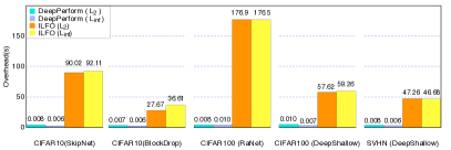
Figure 5. Online overheads to generate one test sample (s)

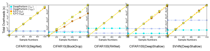
Figure 6. Total overheads of generating different scale test samples (s)

Total Overheads. The total time overheads of generating various scale test samples are shown in Fig. 6. We can see from the results that ILFO is more efficient than DeepPerform when the number of generated test samples is minimal (less than 200). However, when the number of generated test samples grows greater, the overall time overheads of DeepPerform are significantly lower than ILFO. To create 1000 test samples for SN_C10, for example, ILFO will cost five times the overall overheads of DeepPerform. Because the overhead of ILFO is determined by the number of generated test samples (Haque et al., 2020), the total overheads quickly rise as the number of generated test samples rises. The main overhead of DeepPerform, on the other hand, comes from the GAN model training instead of test sample generation. As a result, generating various scale numbers of test samples will have no substantial impact on the DeepPerform’s total overheads. The results imply that ILFO is not scalable for testing AdNNs with large datasets, whereas DeepPerform does an excellent job. We also notice that the DeepPerform’s overheads for $L_{2}$ and $L_{inf}$ are different for DN_SVHN. Because we use the early stopping method (Yao et al., 2007) to train DeepPerform, we can explain such variation in overheads. In detail, the objective $L_{per}$ differs for $L_{2}$ and $L_{inf}$. Thus, training process will terminate at different epochs.

5.3. Effectiveness

5.3.1. Relative Performance Degradation

Metrics. To characterize system performance, we choose both hardware-independent and hardware-dependent metrics. Our hardware independent metric is floating-point operations (FLOPs). FLOPs are widely used to assess the computational complexity of DNNs (Wu et al., 2018; Wang et al., 2018). Higher FLOPs indicate higher CPU utilization and lower efficiency performance. As for hardware-dependent metrics, we focus on latency and energy consumption because these two metrics are essential for real-time applications (Bateni and Liu, 2020; Wan et al., 2020). After characterizing system performance with the above metrics, We measure the increment in the above performance metrics to reflect the severity of performance degradation. In particular, we measure the increased percentage of flops I-FLOPs, latency (I-Latency) and energy consumption (I-Energy) as our performance degradation severity evaluation metrics.

Eq.(9) shows the formal definition of our degradation severity evaluation metrics. In Eq.(9), $x$ is the original seed input, $\delta$ is the generated perturbation, and $F_{f}(\cdot),L_{f}(\cdot),E_{f}(\cdot)$ are the functions that measure FLOPs, latency, and energy consumption of AdNN $f(\cdot)$. A test sample is more effective in triggering performance degradation if it increases more percentage of FLOPs, latency, and energy consumption. We examine two scenarios for each evaluation metric: the average metric value for the whole test dataset and the maximum metric value caused for a particular sample. The first depicts long-term performance degradation, whereas the second depicts performance degradation under the worst-case situation. We measure the energy consumption using TX2’s power monitoring tool (Nvidia, [n. d.]).

(9) $$\begin{split}&I-FLOPs(x)=\frac{F_{f}(x+\delta)-F_{f}(x)}{F_{f}(x)}\times 100\%\\ &I-Latency(x)=\frac{L_{f}(x+\delta)-L_{f}(x)}{L_{f}(x)}\times 100\%\\ &I-Energy(x)=\frac{E_{f}(x+\delta)-E_{f}(x)}{E_{f}(x)}\times 100\%\\ \end{split}$$

Table 4. The FLOPs increment of the test samples (%)

Norm	Subject	Mean		Max
		baseline / ours		baseline / ours
	SN_C10	6.43	31.14	18.43	62.77
	BD_C10	48.44	38.39	162.58	188.60
$L_{inf}$	RN_C100	133.67	181.57	498.29	498.99
	DS_C100	116.19	157.66	287.98	552.00
	DS_SVHN	115.99	228.32	498.29	498.29
	SN_C10	20.34	31.30	30.43	82.09
	BD_C10	48.44	38.39	162.58	188.60
$L_{2}$	RN_C100	133.67	182.12	498.99	498.99
	DS_C100	116.19	157.66	287.98	552.00
	DS_SVHN	115.99	228.32	498.29	498.29

Table 5. The performance degradation on two hardware platforms (%)

Device	Subject	L2								Linf
		I-Latency				I-Energy				I-Latency				I-Energy
		Mean		Max		Mean		Max		Mean		Max		Mean		Max
		baseline/ours		baseline/ours		baseline/ours		baseline/ours		baseline/ours		baseline/ours		baseline/ours		baseline/ours
	SN_C10	8.2	25.4	20.9	45.7	8.3	25.7	20.6	44.9	5.7	30.9	15.1	46.1	5.7	31.4	15.6	45.8
	BD_C10	28.7	17.5	142.1	132.5	28.9	17.7	148.2	135.3	25.4	25.6	143.9	135.7	25.8	26.1	148.2	141.0
CPU	RN_C100	72.2	39.9	1654.4	624.1	72.5	40.3	1685.1	633.7	53.6	141.1	370.2	1313.1	54.1	144.3	387.1	1341.1
	DS_C100	61.4	133.8	216.2	464.0	64.6	142.6	217.3	471.8	52.0	171.5	254.5	483.6	54.9	180.1	282.0	503.9
	DS_SVHN	29.8	210.1	392.3	1496.1	30.3	214.6	398.4	1467.7	70.2	257.2	1371.2	1580.8	71.7	260.1	1372.8	1548.2
	SN_C10	4.4	14.3	6.8	17.9	5.3	15.4	8.1	19.7	4.4	11.8	4.8	15.7	5.2	12.4	6.1	15.9
	BD_C10	9.3	9.8	53.6	41.6	10.2	11.7	59.0	42.4	13.9	16.9	39.9	41.1	15.1	20.2	46.4	46.6
GPU	RN_C100	90.6	51.0	1968.5	923.9	96.9	55.4	2446.5	1043.4	66.9	167.2	454.8	1496.8	70.6	197.4	557.9	1837.4
	DS_C100	56.1	102.7	184.9	370.2	62.8	116.4	194.1	478.8	71.7	158.6	183.8	384.7	80.3	177.9	217.1	457.8
	DS_SVHN	11.5	75.9	149.7	244.2	15.8	92.0	172.3	298.3	38.7	72.0	280.0	308.9	47.4	88.0	348.3	382.8

The hardware-independent experimental results are listed in Table 4. As previously stated, greater I-FLOPs implies that the created test samples demand more FLOPs, which will result in significant system performance reduction. The table concludes that DeepPerform generates test samples that can cause more severe performance degradation. Other than that, we have multiple observations. First, for four of the five subjects, DeepPerform generates test samples that require more FLOPs, e.g., 31.14%-62.77% for SN_C10. Second, for both $L_{2}$ and $L_{inf}$ perturbation, the model would require more FLOPs, and the difference between $L_{2}$ and $L_{inf}$ setting is minimal. Third, the maximum FLOPs are far greater than the average case for some extreme scenarios, e.g., for DS_SVHN, and DS_C100. The hardware-dependent experimental results are listed in Table 5. Similar to hardware-independent experiments, DeepPerform outperforms ILFO on 65 out of 80 comparison scenarios. However, for the other 15 comparisons, we explain the results as the following two reasons: (i) the system noise has affected the results because for almost all scenarios DeepPerform has been able to increase more I-FLOPs than ILFO. (ii) recall in Table 2, $RN\_C100$ has the the PCCs around 0.64, and the FLOPs increment of $RN\_C100$ for DeepPerform and ILFO is around the same level. Thus, DeepPerform may cause slightly less latency and energy consumption degradation than ILFO. However, for $SN\_C10$, although it has low PCCs, DeepPerform can increase much more FLOPs than ILFO, thus, DeepPerform can cause more severe performance degradation. Based on the results in Table 5, we conclude that DeepPerform outperforms baseline in creating inputs that consume higher energy or time.

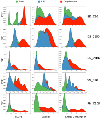
Figure 7. The unnormalized efficiency distribution of seed inputs and the generated inputs

5.3.2. Absolute Performance Degradation

Besides the relative performance degradation, we also investigate the absolute performance degradation of the generated inputs. In Figure 7, we plot the unnormalized efficiency distribution (i.e., FLOPs, latency, energy consumption) of both seed and generated inputs to characterize the absolute performance degradation. We specifically depict the probability distribution function (PDF) curve (James et al., 2013) of each efficiency metric under discussion. The unnormalized efficiency distribution is shown in Fig. 7, where the green curve is for the seed inputs, and the red curve is for the test inputs from DeepPerform. From the results, we observe that DeepPerform is more likely to generate test inputs located at the right end of the x-axis. Recall that a PDF curve with more points on the right end of the x-axis is more likely to generate theoretical worst-case test inputs. The results confirm that DeepPerform is more likely to generate test inputs with theoretical worst-case complexities.

5.3.3. Test Sample Validity

To measure the validity of the generated test samples, we define degradation success number $\eta$ in Eq.(10),

(10) $$\eta=\sum\mathbb{I}(FLOPs(x+\delta)\geq FLOPs(x)).\qquad\qquad x\in\mathcal{X}$$

where $\mathcal{X}$ is the set of randomly selected seed inputs and $\mathbb{I}(FLOPs(x+\delta)>FLOPs(x))$ indicates whether generated test samples require more computational resources than the seed inputs. We run DeepPerform and baselines the same experimental time and generate the different number of test samples ($\mathcal{X}$ in Eq.(10)), we then measure $\eta$ in the generated test samples. For convince, we set the experimental time as the total time of DeepPerform generating 1,000 test samples (same time for ILFO). From the third column in Table 6, we observe that for most experimental settings, DeepPerform achieves a higher degradation success number than ILFO. Although ILFO is an end-to-end approach, the high overheads of ILFO disable it to generate enough test samples.

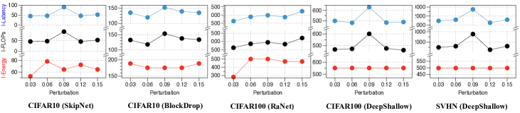
Figure 8. How performance degradation as perturbation constraints change

5.4. Coverage

Table 6. Validity and coverage results

Norm	Subject	$\eta$ (#)		$Cov$ (%)
		ours / baseline		ours / baseline
	SN_C10	842	69	0.74 ± 0.001	0.65 ± 0.001
	BD_C10	630	84	0.37 ± 0.001	0.37 ± 0.001
Linf	RN_C100	871	133	0.99 ± 0.002	0.89 ± 0.030
	DS_C100	646	69	1.00 ± 0.000	0.83 ± 0.016
	DS_SVHN	916	220	1.00 ± 0.000	0.92 ± 0.033
	SN_C10	993	81	0.84 ± 0.001	0.85 ± 0.001
	BD_C10	732	79	0.41 ± 0.001	0.40 ± 0.001
L2	RN_C100	924	229	0.94 ± 0.007	0.95 ± 0.013
	DS_C100	734	181	1.00 ± 0.000	1.00 ± 0.000
	DS_SVHN	924	518	0.98 ± 0.025	0.73 ± 0.034

In this section, we investigate the comprehensiveness of the generated test inputs. In particular, we follow existing work (Pei et al., 2017; Zhang et al., 2018) and investigate the diversity of the AdNN behaviors explored by the test inputs generated by DeepPerform. Because AdNNs’ behavior relies on the computation of intermediate states (Pei et al., 2017; Ma et al., 2018), we analyze how many intermediate states are covered by the test suite.

(11) $$\quad Cov(\mathcal{X})=\frac{\sum_{x\in\mathcal{X}}\sum_{i=1}^{N}\mathbb{I}(B_{i}(x)>\tau_{i}))}{N}$$

To measure the coverage of AdNNs’ intermediate states, we follow existing work (Pei et al., 2017) and define decision block coverage ($Cov(\mathcal{X})$ in Eq.(11)), where $N$ is the total number blocks, $\mathbb{I}(\cdot)$ is the indicator function, and $(B_{i}(x)>\tau_{i}))$ represents whether $i^{th}$ block is activated by input $x$ (the definition of $B_{i}$ and $\tau_{i}$ are the same with Eq.(1) and Eq.(2)). Because AdNNs activate different blocks for decision making, then a higher block coverage indicates the test samples cover more decision behaviors. For each subject, we randomly select 100 seed samples from the test dataset as seed inputs. We then feed the same seed inputs into DeepPerform and ILFO to generate test samples. Finally, we feed the generated test samples to AdNNs and measure block coverage. We repeat the process ten times and record the average coverage and the variance. The results are shown in Table 6 last two columns. We observe that the test samples generated by DeepPerform achieve higher coverage for almost all subjects.

5.5. Sensitivity

In this section, we conduct two experiments to show that DeepPerform can generate effective test samples under different settings.

Configuration Sensitivity. As discussed in §2, AdNNs require configuring the threshold $\tau_{i}$ to set the accuracy-performance tradeoff mode. In this section, we evaluate whether the test samples generated from DeepPerform could degrade the AdNNs’ performance under different modes. Specifically, we set the threshold $\tau_{i}$ in Eq.(1) and Eq.(2) as $0.3,0.4,0.5,0.6,0.7$ and measure the maximum FLOPs increments. Notice that we train DeepPerform with $\tau_{i}=0.5$ and test the performance degradation with different $\tau_{i}$. The maximum FLOPs increment ratio under different system configurations are listed in Table 7. For all experimental settings, the maximum FLOPs increment ratio keeps a stable value (e.g., 79.17-82.91, 175.59-250.00). The results imply that the test samples generated by DeepPerform can increase the computational complexity under different configurations, and the maximum FLOPs increment ratio is stable as the configuration changes.

Table 7. Increment under different thresholds

Norm	Subject	Threshold
		0.3	0.4	0.5	0.6	0.7
	SN_C10	79.17	82.91	82.91	75.00	70.00
	BD_C10	250.00	250.00	175.59	175.59	175.59
L2	RN_C100	500.00	498.99	498.99	200.00	200.00
	DS_C100	600.00	600.00	552.00	400.00	200.00
	DS_SVHN	498.29	498.29	498.29	498.29	400.00
	SN_C10	66.67	78.26	82.91	66.67	73.91
	BD_C10	233.33	175.59	175.59	233.33	233.33
Linf	RN_C100	498.99	498.99	498.99	498.99	498.99
	DS_C100	552.00	552.00	552.00	400.00	300.00
	DS_SVHN	498.29	498.29	498.29	498.29	400.00

Table 8. Performance degradation on different hardware

Norm	Subject	Intel Xeon E5-2660 v3 CPU		Nvidia 1080 Ti
		I-Latency / I-Energy		I-Latency / I-Energy
	SN_C10	36.95	36.20	24.94	50.77
	BD_C10	76.69	79.24	64.10	63.55
L2	RN_C100	1019.25	1173.21	938.21	856.46
	DS_C100	567.10	609.73	414.38	338.51
	DS_SVHN	236.12	246.70	311.01	282.09
	SN_C10	29.38	28.28	24.95	11.94
	BD_C10	70.67	74.09	49.82	52.70
Linf	RN_C100	319.72	355.29	679.79	652.98
	DS_C100	463.91	496.84	439.53	464.65
	DS_SVHN	232.88	244.91	263.49	141.56

Hardware Sensitivity. We next evaluate the effectiveness of our approach on different hardware platforms. In particular, we select Intel Xeon E5-2660 V3 CPU and Nvidia 1080 Ti as our experimental hardware platforms and measure the maximum performance degradation ratio on those selected platforms. The test samples generated by DeepPerform, as shown in Table 8, cause severe and stable runtime performance degradation on different hardware platforms. As a result, we conclude that DeepPerform is not sensitive to hardware platforms.

5.6. Quality

Table 9. The perturbation size of the generated test inputs

Norm	SN_C10	BD_C10	RN_C100	DS_C100	DS_SVHN
L2	9.48	9.47	9.50	9.48	9.62
Linf	0.03	0.03	0.03	0.03	0.03

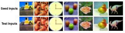
Figure 9. Testing inputs generated by DeepPerform

We first conduct quantitative evaluations to evaluate the similarity between the generated and seed inputs. In particular, we follow existing work (Carlini and Wagner, 2017) and compute the perturbation magnitude. The perturbation magnitude are listed in Table 9. Recall that we follow existing work (Carlini and Wagner, 2017; Haque et al., 2020) and set the perturbation constraints $\epsilon$ as $10$ and $0.03$ for $L_{2}$ and $L_{inf}$ norm (§5.1). From the results in Table 9, we conclude that generated test samples can satisfy the semantic-equivalent constraints in Eq.(3). Moreover, we conduct a qualitative evaluation. In particular, we randomly select seven images from the generated images for RA_C100 and visualize them in Fig. 9 (more results are available on our website), where the first row is the randomly selected seed inputs, and the second row is the corresponding generated inputs. The visualization results show that the test inputs generated by DeepPerform are semantic-equivalent to the seed inputs. Furthermore, we investigate the relationship between different semantic-equivalent constraints and performance degradation. We first change the perturbation magnitude constraints (i.e., $\eta$ in Eq.(3)) and train different models (experiment results for $L_{2}$ norm could be found on our websites). After that, we measure the severity of AdNN performance degradation under various settings. Fig. 8 shows the results. We observe that although the relationship between performance degradation ratio and perturbation magnitude is not purely linear, there is a trend that the overhead increases with the increase of perturbation magnitude.

Table 10. Efficiency and accuracy of AdNN model

Metric		SN_C10	BD_C10	RN_C100	DS_C100	DS_SVHN
I-FLOPs	before	31.30	38.39	182.12	157.66	228.32
	after	8.07	15.26	35.37	28.54	38.65
Acc	before	92.34	91.35	65.43	58.78	94.54
	after	13.67	10.56	6.67	7.67	18.78

6. Application

This section investigates if developers can mitigate the performance degradation bugs using the existing methods for mitigating DNN correctness bugs (i.e., adversarial examples). We focus on two of the most widely employed approaches: offline adversarial training (Goodfellow et al., 2015), and online input validation (Wang et al., 2020). Surprisingly, we discover that not all of the two approaches can address performance faults in the same manner they are used to repair correctness bugs.

6.1. Adversarial Training

Setup. We follow existing work (Goodfellow et al., 2015) and feed the generated test samples and the original model training data to retrain each AdNN. The retraining objective can be formulated as

(12) $$\mathcal{L}_{retrain}=\underbrace{\ell(g_{f}(x^{\prime}),\;g_{f}(x))}_{\mathcal{L}_{1}}+\underbrace{\beta\left\{\ell(f(x),y)+\ell(f(x^{\prime}),y)\right\}}_{\mathcal{L}_{2}}$$

where $x$ is one seed input in the training dataset, $x^{\prime}=\mathcal{G}(x)+x$ is the generated test input, $f(\cdot)$ is the AdNNs, and $g_{f}(\cdot)$ measures the AdNNs computational FLOPs. Our retraining objective can be interpreted as forcing the buggy test inputs $x^{\prime}$ to consume the same FLOPs as the seed one (i.e., $\mathcal{L}_{1}$), while producing the correct results (i.e., $\mathcal{L}_{2}$). For each AdNN model under test, we retrain it to minimize the objective in Eq.(12). After retraining, we test each AdNNs accuracy and efficiency on the hold-out test dataset.

Results. Table 10 shows the results after model retraining. The left two columns show the performance degradation before and after model retraining, while the right two columns show the model accuracy before and after model retraining. The findings show that following model training, the I-FLOPs fall; keep in mind that a higher I-FLOPs signifies a more severe performance degradation. Thus, the decrease in I-FLOPs implies that model retraining can help overcome performance degradation. However, based on the data in the right two columns, we observe that such retraining, different from accuracy-based retraining, may harm model accuracy.

Table 11. Performance of SVM detector

Subject	AUC		Extra Latency (s)		Extra Energy (j)
	L2	Linf	L2	Linf	L2	Linf
SN_C10	0.9997	0.9637	0.0168	0.0167	1.8690	1.8740
BD_C10	0.9967	0.9222	0.0001	0.0002	0.0108	0.0197
RN_C100	1.0000	0.9465	0.0031	0.0042	0.3263	0.4658
DS_C100	0.5860	0.3773	0.0167	0.0212	1.8578	2.4408
DS_SVHN	1.0000	1.0000	0.0098	0.0210	1.1030	2.3959

6.2. Input Validation

Input validation (Wang et al., 2020) is a runtime approach that filters out abnormal inputs before AdNNs cast computational resources on such abnormal inputs. This approach is appropriate for situations where the sensors (e.g., camera) and the decision system (e.g., AdNN) work at separate frequencies. Such different frequency working mode is very common in robotics systems (Luo and Yuille, 2019; Feichtenhofer et al., 2019; Zolfaghari et al., 2018), where the AdNN system will randomly select one image from continuous frames from sensors since continuous frames contain highly redundant information. Our intuition is to filter out those abnormal inputs at the early computational stage, the same as previous work (Wang et al., 2020).

Design of Input Filtering Detector. Our idea is that although seed inputs and the generated test inputs look similar, the latent representations of these two category inputs are quite different (Wang et al., 2020). Thus, we extract the hidden representation of a given input by running the first convolutional layer of the AdNNs. First, we feed both benign and DeepPerform generated test inputs to specific AdNN. We use the outputs of the first convolutional layer as input to train a linear SVM to classify benign inputs and inputs that require huge computation. If any resource consuming adversarial input is detected, the inference is stopped. The computational complexity of the SVM detector is significantly less than AdNNs. Thus the detector will not induce significant computational resources consumption.

Setup. For each experimental subject, we randomly choose 1,000 seed samples from the training dataset, and apply DeepPerform to generate 1,000 test samples. We use these 2,000 inputs to train our detector. To evaluate the performance of our detector, we first randomly select 1,000 inputs from the test dataset and apply DeepPerform to generate 1000 test samples. After that, we run the trained detector on such 2,000 inputs and measure detectors’ AUC score, extra computation overheads, and energy consumption.

Results. Table 11 shows that the trained SVM detector can successfully detect the test samples that require substantial computational resources. Specifically for $L_{2}$ norm perturbation, all the AUC scores are higher than 0.99. The results indicate that the proposed detector identifies $L_{2}$ test samples better. The last four columns show the extra computational resources consumption of the detector. We observe that the detector does not consume many additional computational resources from the results.

7. Threats To Validity

Our selection of five experimental subjects might be the external threat that threaten the generability of our conclusions. We alleviate this threat by the following efforts. (1) We ensure that the datasets are widely used in both academia and industry research. (2) All evaluated models are state-of-the-art DNN models (published in top-tier conferences after 2017). (3) Our subjects are diverse in terms of a varied set of topics: all of our evaluated datasets and models differ from each other in terms of different input domains (e.g., digit, general object recognition), the number of classes (from 10 to 100), the size of the training dataset (from 50,000 to 73,257), the model adaptive mechanism. Our internal threat mainly comes from the realism of the generated inputs. We alleviate this threat by demonstrating the relationship of our work with existing work. Existing work (Zhang et al., 2018; Zhou et al., 2020; Kurakin et al., 2017) demonstrates that correctness-based test inputs exist in the physical world. Because we formulate our problem(i.e., the constraint in Eq.(3)) the same as the previous correctness-based work (Zhou et al., 2020; Madry et al., 2018), we conclude our generated test samples are real and exist in the physical world.

8. Related Works

Adversarial Examples & DNN Testing. Adversarial Examples have been used evaluate the robustness of DNNs. These examples are fed to DNNs to change the prediction of the model. Szegedy et al. (Szegedy et al., 2014) and Goodfellow et al. (Goodfellow et al., 2015) propose adversarial attacks on DNNs. Karmon et al. Adversarial attacks have been extended to various fields like natural language and speech processing (Carlini et al., 2016; Jia and Liang, 2017), and graph models (Zügner et al., 2018; Bojchevski and Günnemann, 2019). Although, all these attacks focus on changing the prediction and do not concentrate on performance testing. Several testing methods have been proposed to test DNNs (Zhang et al., 2018; Zhou et al., 2020; Chen et al., 2022, 2021).

Performance Testing. Runtime performance is a critical property of software, and a branch of work has been proposed to test software performance. For example, Netperf (HP, [n. d.]) and IOZone (W. Norcott and D. Capps, [n. d.]) evaluate the performance of different virtual machine technologies. WISE (Burnim et al., 2009) proposes a method to generate test samples to trigger worst-case complexity. SlowFuzz (Petsios et al., 2017) proposes a fuzzing framework to detect algorithmic complexity vulnerabilities. PerfFuzz (Lemieux et al., 2018) generates inputs that trigger pathological behavior across program locations.

9. Conclusion

In this paper, we propose DeepPerform, a performance testing framework for DNNs. Specifically, DeepPerform trains a GAN to learn and approximate the distribution of the samples that require more computational units. Through our evaluation, we have shown that DeepPerform is able to find IDPB in AdNNs more effectively and efficiently than baseline techniques.

- (1)
- Athalye et al. (2018) Anish Athalye, Nicholas Carlini, and David A. Wagner. 2018. Obfuscated Gradients Give a False Sense of Security: Circumventing Defenses to Adversarial Examples. In Proceedings of the 35th International Conference on Machine Learning, ICML 2018. PMLR, 274–283.
- Bateni and Liu (2018) Soroush Bateni and Cong Liu. 2018. Apnet: Approximation-aware real-time neural network. In 2018 IEEE Real-Time Systems Symposium, RTSS 2018. IEEE Computer Society, 67–79.
- Bateni and Liu (2020) Soroush Bateni and Cong Liu. 2020. NeuOS: A Latency-Predictable Multi-Dimensional Optimization Framework for DNN-driven Autonomous Systems. In 2020 USENIX Annual Technical Conference, USENIX ATC 2020. USENIX Association, 371–385.
- Bojchevski and Günnemann (2019) Aleksandar Bojchevski and Stephan Günnemann. 2019. Adversarial Attacks on Node Embeddings via Graph Poisoning. In Proceedings of the 36th International Conference on Machine Learning, ICML 2019. PMLR, 695–704.
- Bolukbasi et al. (2017) Tolga Bolukbasi, Joseph Wang, Ofer Dekel, and Venkatesh Saligrama. 2017. Adaptive Neural Networks for Efficient Inference. In Proceedings of the 34th International Conference on Machine Learning, ICML 2017. PMLR, 527–536.
- Burnim et al. (2009) Jacob Burnim, Sudeep Juvekar, and Koushik Sen. 2009. WISE: Automated test generation for worst-case complexity. In 31st International Conference on Software Engineering, ICSE 2009. IEEE, 463–473.
- Carlini et al. (2016) Nicholas Carlini, Pratyush Mishra, Tavish Vaidya, Yuankai Zhang, Micah Sherr, Clay Shields, David A. Wagner, and Wenchao Zhou. 2016. Hidden Voice Commands. In 25th USENIX Security Symposium, USENIX Security 2016. USENIX Association, 513–530.
- Carlini and Wagner (2017) Nicholas Carlini and David A. Wagner. 2017. Towards Evaluating the Robustness of Neural Networks. In 2017 IEEE Symposium on Security and Privacy, SP 2017. IEEE Computer Society, 39–57.
- Chan et al. (2016) William Chan, Navdeep Jaitly, Quoc V. Le, and Oriol Vinyals. 2016. Listen, attend and spell: A neural network for large vocabulary conversational speech recognition. In 2016 IEEE International Conference on Acoustics, Speech and Signal Processing, ICASSP 2016. IEEE, 4960–4964.
- Chen et al. (2021) Simin Chen, Mirazul Haque, Zihe Song, Cong Liu, and Wei Yang. 2021. Transslowdown: Efficiency Attacks on Neural Machine Translation Systems. OpenReview.net.
- Chen et al. (2022) Simin Chen, Zihe Song, Mirazul Haque, Cong Liu, and Wei Yang. 2022. NICGSlowDown: Evaluating the Efficiency Robustness of Neural Image Caption Generation Models. In Proceedings of the IEEE/CVF Conference on Computer Vision and Pattern Recognition (CVPR). IEEE, 15365–15374.
- Davis and Arel (2014) Andrew S. Davis and Itamar Arel. 2014. Low-Rank Approximations for Conditional Feedforward Computation in Deep Neural Networks. In 2nd International Conference on Learning Representations, ICLR 2014.
- Feichtenhofer et al. (2019) Christoph Feichtenhofer, Haoqi Fan, Jitendra Malik, and Kaiming He. 2019. SlowFast Networks for Video Recognition. In 2019 IEEE/CVF International Conference on Computer Vision, ICCV 2019. IEEE, 6201–6210.
- Gao et al. (2018) Mingfei Gao, Ruichi Yu, Ang Li, Vlad I. Morariu, and Larry S. Davis. 2018. Dynamic Zoom-In Network for Fast Object Detection in Large Images. In 2018 IEEE Conference on Computer Vision and Pattern Recognition, CVPR 2018. Computer Vision Foundation / IEEE Computer Society, 6926–6935.
- Goodfellow et al. (2015) Ian J. Goodfellow, Jonathon Shlens, and Christian Szegedy. 2015. Explaining and Harnessing Adversarial Examples. In 3rd International Conference on Learning Representations, ICLR 2015.
- Han et al. (2015) Song Han, Huizi Mao, and William J Dally. 2015. Deep Compression: Compressing Deep neural Networks with Pruning, Trained Quantization and Huffman Coding. arXiv preprint arXiv:1510.00149 (2015).
- Haque et al. (2020) Mirazul Haque, Anki Chauhan, Cong Liu, and Wei Yang. 2020. ILFO: Adversarial Attack on Adaptive Neural Networks. In Proceedings of the IEEE/CVF Conference on Computer Vision and Pattern Recognition, CVPR 2020. IEEE, 14252–14261.
- HP ([n. d.]) HP. [n. d.]. Netperf. http://www.netperf.org.
- Hua et al. (2019) Weizhe Hua, Yuan Zhou, Christopher De Sa, Zhiru Zhang, and G. Edward Suh. 2019. Channel Gating Neural Networks. In Advances in Neural Information Processing Systems 32: Annual Conference on Neural Information Processing Systems 2019, NeurIPS 2019. 1884–1894.
- Huang et al. (2018) Rachel Huang, Jonathan Pedoeem, and Cuixian Chen. 2018. YOLO-LITE: A Real-Time Object Detection Algorithm Optimized for Non-GPU Computers. In IEEE International Conference on Big Data (IEEE BigData 2018). IEEE, 2503–2510.
- James et al. (2013) Gareth James, Daniela Witten, Trevor Hastie, and Robert Tibshirani. 2013. An introduction to statistical learning. Vol. 112. Springer.
- Jia and Liang (2017) Robin Jia and Percy Liang. 2017. Adversarial Examples for Evaluating Reading Comprehension Systems. In Proceedings of the 2017 Conference on Empirical Methods in Natural Language Processing, EMNLP 2017. Association for Computational Linguistics, 2021–2031.
- Jiang et al. (2021) Shiqi Jiang, Zhiqi Lin, Yuanchun Li, Yuanchao Shu, and Yunxin Liu. 2021. Flexible high-resolution object detection on edge devices with tunable latency. In The 27th Annual International Conference on Mobile Computing and Networking,ACM MobiCom 2021. ACM, 559–572.
- Kaya et al. (2019) Yigitcan Kaya, Sanghyun Hong, and Tudor Dumitras. 2019. Shallow-Deep Networks: Understanding and Mitigating Network Overthinking. In Proceedings of the 36th International Conference on Machine Learning, ICML 2019. PMLR, 3301–3310.
- Krizhevsky et al. (2009) Alex Krizhevsky, Geoffrey Hinton, et al. 2009. Learning multiple layers of features from tiny images. arXiv preprint arXiv:1805.12549 (2009).
- Kurakin et al. (2017) Alexey Kurakin, Ian J. Goodfellow, and Samy Bengio. 2017. Adversarial examples in the physical world. In 5th International Conference on Learning Representations, ICLR 2017. OpenReview.net.
- Lemieux et al. (2018) Caroline Lemieux, Rohan Padhye, Koushik Sen, and Dawn Song. 2018. PerfFuzz: automatically generating pathological inputs. In Proceedings of the 27th ACM SIGSOFT International Symposium on Software Testing and Analysis, ISSTA 2018, Frank Tip and Eric Bodden (Eds.). ACM, 254–265.
- Li et al. (2019) Shasha Li, Ajaya Neupane, Sujoy Paul, Chengyu Song, Srikanth V. Krishnamurthy, Amit K. Roy-Chowdhury, and Ananthram Swami. 2019. Stealthy Adversarial Perturbations Against Real-Time Video Classification Systems. In 26th Annual Network and Distributed System Security Symposium, NDSS 2019. The Internet Society.
- Lin et al. (2017) Ji Lin, Yongming Rao, Jiwen Lu, and Jie Zhou. 2017. Runtime Neural Pruning. In Advances in Neural Information Processing Systems 30: Annual Conference on Neural Information Processing Systems 2017. 2181–2191.
- Liu and Deng (2018) Lanlan Liu and Jia Deng. 2018. Dynamic Deep Neural Networks: Optimizing Accuracy-Efficiency Trade-Offs by Selective Execution. In Proceedings of the Thirty-Second AAAI Conference on Artificial Intelligence, (AAAI-18), the 30th innovative Applications of Artificial Intelligence (IAAI-18), and the 8th AAAI Symposium on Educational Advances in Artificial Intelligence (EAAI-18). AAAI Press, 3675–3682.
- Luo and Yuille (2019) Chenxu Luo and Alan L. Yuille. 2019. Grouped Spatial-Temporal Aggregation for Efficient Action Recognition. In 2019 IEEE/CVF International Conference on Computer Vision, ICCV 2019. IEEE, 5511–5520.
- Ma et al. (2018) Lei Ma, Felix Juefei-Xu, Fuyuan Zhang, Jiyuan Sun, Minhui Xue, Bo Li, Chunyang Chen, Ting Su, Li Li, Yang Liu, et al. 2018. Deepgauge: Multi-granularity testing criteria for deep learning systems. In Proceedings of the 33rd ACM/IEEE International Conference on Automated Software Engineering, ASE 2018. ACM, 120–131.
- Madry et al. (2018) Aleksander Madry, Aleksandar Makelov, Ludwig Schmidt, Dimitris Tsipras, and Adrian Vladu. 2018. Towards Deep Learning Models Resistant to Adversarial Attacks. In 6th International Conference on Learning Representations, ICLR 2018. OpenReview.net.
- Najibi et al. (2019) Mahyar Najibi, Bharat Singh, and Larry Davis. 2019. AutoFocus: Efficient Multi-Scale Inference. In 2019 IEEE/CVF International Conference on Computer Vision, ICCV 2019. IEEE, 9744–9754.
- Nan and Saligrama (2017) Feng Nan and Venkatesh Saligrama. 2017. Adaptive Classification for Prediction Under a Budget. In Advances in Neural Information Processing Systems 30: Annual Conference on Neural Information Processing Systems 2017. 4727–4737.
- Netzer et al. (2011) Yuval Netzer, Tao Wang, Adam Coates, Alessandro Bissacco, Bo Wu, and Andrew Y Ng. 2011. Reading digits in natural images with unsupervised feature learning. arXiv preprint arXiv:1503.02531 (2011).
- Nvidia ([n. d.]) Nvidia. [n. d.]. Jetson TX2 Module. %****␣main.bbl␣Line␣475␣****https://developer.nvidia.com/embedded/jetson-tx2.
- Pei et al. (2017) Kexin Pei, Yinzhi Cao, Junfeng Yang, and Suman Jana. 2017. DeepXplore: Automated Whitebox Testing of Deep Learning Systems. In Proceedings of the 26th Symposium on Operating Systems Principles, SOSP 2017. ACM, 1–18.
- Petsios et al. (2017) Theofilos Petsios, Jason Zhao, Angelos D. Keromytis, and Suman Jana. 2017. SlowFuzz: Automated Domain-Independent Detection of Algorithmic Complexity Vulnerabilities. In Proceedings of the 2017 ACM SIGSAC Conference on Computer and Communications Security, CCS 2017. ACM, 2155–2168.
- Rice (2006) John A Rice. 2006. Mathematical statistics and data analysis. arXiv preprint arXiv:1503.02531 (2006).
- Shazeer et al. (2017) Noam Shazeer, Azalia Mirhoseini, Krzysztof Maziarz, Andy Davis, Quoc V. Le, Geoffrey E. Hinton, and Jeff Dean. 2017. Outrageously Large Neural Networks: The Sparsely-Gated Mixture-of-Experts Layer. In 5th International Conference on Learning Representations, ICLR 2017. OpenReview.net.
- Szegedy et al. (2014) Christian Szegedy, Wojciech Zaremba, Ilya Sutskever, Joan Bruna, Dumitru Erhan, Ian J. Goodfellow, and Rob Fergus. 2014. Intriguing properties of neural networks. In 2nd International Conference on Learning Representations, ICLR 2014. Openreview.net.
- Tang et al. (2021) Xiaohu Tang, Shihao Han, Li Lyna Zhang, Ting Cao, and Yunxin Liu. 2021. To Bridge Neural Network Design and Real-World Performance: A Behaviour Study for Neural Networks. In Proceedings of Machine Learning and Systems 2021, MLSys 2021. mlsys.org.
- Teerapittayanon et al. (2016) Surat Teerapittayanon, Bradley McDanel, and H. T. Kung. 2016. BranchyNet: Fast inference via early exiting from deep neural networks. In 23rd International Conference on Pattern Recognition, ICPR 2016. IEEE, 2464–2469.
- Tian et al. (2018) Yuchi Tian, Kexin Pei, Suman Jana, and Baishakhi Ray. 2018. Deeptest: Automated testing of deep-neural-network-driven autonomous cars. In Proceedings of the 40th international conference on software engineering ASE 2018. ACM, 303–314.
- Vaswani et al. (2017) Ashish Vaswani, Noam Shazeer, Niki Parmar, Jakob Uszkoreit, Llion Jones, Aidan N. Gomez, Lukasz Kaiser, and Illia Polosukhin. 2017. Attention is All you Need. In Advances in Neural Information Processing Systems 30: Annual Conference on Neural Information Processing Systems 2017. 5998–6008.
- Veit and Belongie (2018) Andreas Veit and Serge J. Belongie. 2018. Convolutional Networks with Adaptive Inference Graphs. In Proceedings of the European conference on computer vision (ECCV 2018). Springer, 3–18.
- W. Norcott and D. Capps ([n. d.]) W. Norcott and D. Capps. [n. d.]. IOZone. http://www.iozone.org/.
- Wan et al. (2020) Chengcheng Wan, Muhammad Santriaji, Eri Rogers, Henry Hoffmann, Michael Maire, and Shan Lu. 2020. ALERT: Accurate Learning for Energy and Timeliness. In 2020 USENIX Annual Technical Conference (USENIX ATC 20). USENIX Association, 353–369.
- Wang et al. (2020) Huiyan Wang, Jingwei Xu, Chang Xu, Xiaoxing Ma, and Jian Lu. 2020. Dissector: Input validation for deep learning applications by crossing-layer dissection. In 2020 IEEE/ACM 42nd International Conference on Software Engineering (ICSE 2020). IEEE, 727–738.
- Wang et al. (2021) Manni Wang, Shaohua Ding, Ting Cao, Yunxin Liu, and Fengyuan Xu. 2021. AsyMo: scalable and efficient deep-learning inference on asymmetric mobile CPUs. In Proceedings of the 27th Annual International Conference on Mobile Computing and Networking (ACM MobiCom 2021). ACM, 215–228.
- Wang et al. (2018) Xin Wang, Fisher Yu, Zi-Yi Dou, Trevor Darrell, and Joseph E. Gonzalez. 2018. SkipNet: Learning Dynamic Routing in Convolutional Networks. In Proceedings of the European conference on computer vision (ECCV 2018). Springer, 420–436.
- Wu et al. (2018) Zuxuan Wu, Tushar Nagarajan, Abhishek Kumar, Steven Rennie, Larry S Davis, Kristen Grauman, and Rogerio Feris. 2018. Blockdrop: Dynamic inference paths in residual networks. In 2018 IEEE Conference on Computer Vision and Pattern Recognition, CVPR 2018. Computer Vision Foundation / IEEE Computer Society, 8817–8826.
- Wu et al. (2019) Zuxuan Wu, Caiming Xiong, Chih-Yao Ma, Richard Socher, and Larry S. Davis. 2019. AdaFrame: Adaptive Frame Selection for Fast Video Recognition. In IEEE Conference on Computer Vision and Pattern Recognition, CVPR 2019. Computer Vision Foundation / IEEE, 1278–1287.
- Xiao et al. (2013) Xusheng Xiao, Shi Han, Dongmei Zhang, and Tao Xie. 2013. Context-sensitive delta inference for identifying workload-dependent performance bottlenecks. In International Symposium on Software Testing and Analysis, ISSTA 2013. ACM, 90–100.
- Yang et al. (2020) Le Yang, Yizeng Han, Xi Chen, Shiji Song, Jifeng Dai, and Gao Huang. 2020. Resolution Adaptive Networks for Efficient Inference. In 2020 IEEE/CVF Conference on Computer Vision and Pattern Recognition, CVPR 2020. Computer Vision Foundation / IEEE, 2366–2375.
- Yao et al. (2007) Y Yao, L Rosasco, A Caponnetto Constructive Approximation, and undefined 2007. 2007. On early stopping in gradient descent learning. Constructive Approximation 26 (2007), 289–315.
- Zhang et al. (2018) Mengshi Zhang, Yuqun Zhang, Lingming Zhang, Cong Liu, and Sarfraz Khurshid. 2018. DeepRoad: GAN-based metamorphic testing and input validation framework for autonomous driving systems. In 2018 33rd IEEE/ACM International Conference on Automated Software Engineering (ASE 2018). ACM, 132–142.
- Zhou et al. (2020) Husheng Zhou, Wei Li, Zelun Kong, Junfeng Guo, Yuqun Zhang, Bei Yu, Lingming Zhang, and Cong Liu. 2020. Deepbillboard: Systematic physical-world testing of autonomous driving systems. In 2020 IEEE/ACM 42nd International Conference on Software Engineering (ICSE 2020). IEEE, 347–358.
- Zolfaghari et al. (2018) Mohammadreza Zolfaghari, Kamaljeet Singh, and Thomas Brox. 2018. Eco: Efficient convolutional network for online video understanding. In Proceedings of the European conference on computer vision (ECCV 2018). Springer, 695–712.
- Zügner et al. (2018) Daniel Zügner, Amir Akbarnejad, and Stephan Günnemann. 2018. Adversarial Attacks on Neural Networks for Graph Data. In Proceedings of the 24th ACM SIGKDD International Conference on Knowledge Discovery & Data Mining, KDD 2018. ACM, 2847–2856.