Learning Explicit Credit Assignment for Cooperative Multi-Agent Reinforcement Learning via Polarization Policy Gradient

Abstract

Cooperative multi-agent policy gradient (MAPG) algorithms have recently attracted wide attention and are regarded as a general scheme for the multi-agent system. Credit assignment plays an important role in MAPG and can induce cooperation among multiple agents. However, most MAPG algorithms cannot achieve good credit assignment because of the game-theoretic pathology known as centralized-decentralized mismatch. To address this issue, this paper presents a novel method, Multi-Agent Polarization Policy Gradient (MAPPG). MAPPG takes a simple but efficient polarization function to transform the optimal consistency of joint and individual actions into easily realized constraints, thus enabling efficient credit assignment in MAPG. Theoretically, we prove that individual policies of MAPPG can converge to the global optimum. Empirically, we evaluate MAPPG on the well-known matrix game and differential game, and verify that MAPPG can converge to the global optimum for both discrete and continuous action spaces. We also evaluate MAPPG on a set of StarCraft II micromanagement tasks and demonstrate that MAPPG outperforms the state-of-the-art MAPG algorithms.

1 Introduction

Multi-agent reinforcement learning (MARL) is a critical learning technology to solve sequential decision problems with multiple agents. Recent developments in MARL have heightened the need for fully cooperative MARL that maximizes a reward shared by all agents. Cooperative MARL has made remarkable advances in many domains, including autonomous driving (Cao et al. 2021) and cooperative transport (Shibata, Jimbo, and Matsubara 2021). To mitigate the combinatorial nature (Hernandez-Leal, Kartal, and Taylor 2019) and partial observability (Omidshafiei et al. 2017) in MARL, centralized training with decentralized execution (CTDE) (Oliehoek, Spaan, and Vlassis 2008; Kraemer and Banerjee 2016) has become one of the mainstream settings for MARL, where global information is provided to promote collaboration in the training phase and learned policies are executed only based on local observations.

Multi-agent credit assignment is a crucial challenge in the MARL under the CTDE setting, which refers to attributing a global environmental reward to the individual agents’ actions (Zhou et al. 2020). Multiple independent agents can learn effective collaboration policies to accomplish challenging tasks with the proper credit assignment. MARL algorithms can be divided into value-based and policy-based. Cooperative multi-agent policy gradient (MAPG) algorithms can handle both discrete and continuous action spaces, which is the focus of our study. Different MAPG algorithms adopt different credit assignment paradigms, which can be divided into implicit and explicit credit assignment (Zhou et al. 2020). Solving the credit assignment problem implicitly needs to represent the joint action value as a function of individual policies (Lowe et al. 2017; Zhou et al. 2020; Wang et al. 2021b; Zhang et al. 2021; Peng et al. 2021). Current state-of-the-art MAPG algorithms (Wang et al. 2021b; Zhang et al. 2021; Peng et al. 2021) impose a monotonic constraint between the joint action value and individual policies. While some algorithms allow more expressive value function classes, the capacity of the value mixing network is still limited by the monotonic constraints (Son et al. 2019; Wang et al. 2021a). The other algorithms that achieve explicit credit assignment mainly provide a shaped reward for each individual agent’s action (Proper and Tumer 2012; Foerster et al. 2018; Su, Adams, and Beling 2021). However, there is a large discrepancy between the performance of algorithms with explicit credit assignment and algorithms with implicit credit assignment.

In this paper, we analyze this discrepancy and pinpoint that the centralized-decentralized mismatch hinders the performance of MAPG algorithms with explicit credit assignment. The centralized-decentralized mismatch can arise when the sub-optimal policies of agents could negatively affect the assessment of other agents’ actions, which leads to catastrophic miscoordination. Note that the issue of centralized-decentralized mismatch was raised by DOP (Wang et al. 2021b). However, the linearly decomposed critic adopted by DOP (Wang et al. 2021b) limits their representation expressiveness for the value function.

Inspired by Polarized-VAE (Balasubramanian et al. 2021) and Weighted QMIX (Rashid et al. 2020), we propose a policy-based algorithm called Multi-Agent Polarization Policy Gradient (MAPPG) for learning explicit credit assignment to address the centralized-decentralized mismatch. MAPPG encourages increasing the distance between the global optimal joint action value and the non-optimal joint action values while shortening the distance between multiple non-optimal joint action values via polarization policy gradient. MAPPG facilitates large-scale multi-agent cooperations and presents a new multi-agent credit assignment paradigm, enabling multi-agent policy learning like single-agent policy learning (Wei and Luke 2016). Theoretically, we prove that individual policies of MAPPG can converge to the global optimum. Empirically, we verify that MAPPG can converge to the global optimum compared to existing MAPG algorithms in the well-known matrix (Son et al. 2019) and differential games (Wei et al. 2018). We also show that MAPPG outperforms the state-of-the-art MAPG algorithms on StarCraft II unit micromanagement tasks (Samvelyan et al. 2019), demonstrating its scalability in complex scenarios. Finally, the results of ablation experiments match our theoretical predictions.

2 Related Work

Implicit Credit Assignment

In general, implicit MAPG algorithms utilize the learned function between the individual policies and the joint action values for credit assignment. MADDPG (Lowe et al. 2017) and LICA (Zhou et al. 2020) learn the individual policies by directly ascending the approximate joint action value gradients. The state-of-the-art MAPG algorithms (Wang et al. 2021b; Zhang et al. 2021; Peng et al. 2021; Su, Adams, and Beling 2021) introduce the idea of value function decomposition (Sunehag et al. 2018; Rashid et al. 2018; Son et al. 2019; Wang et al. 2021a; Rashid et al. 2020) into the multi-agent actor-critic framework. DOP (Wang et al. 2021b) decomposes the centralized critic as a weighted linear summation of individual critics that condition local actions. FOP (Zhang et al. 2021) imposes a multiplicative form between the optimal joint policy and the individual optimal policy, and optimizes both policies based on maximum entropy reinforcement learning objectives. FACMAC (Peng et al. 2021) proposes a new credit-assignment actor-critic framework that factors the joint action value into individual action values and uses the centralized gradient estimator for credit assignment. VDAC (Su, Adams, and Beling 2021) achieves the credit assignment by enforcing the monotonic relationship between the joint action values and the shaped individual action values. Although these algorithms allow more expressive value function classes, the capacity of the value mixing network is still limited by the monotonic constraints, and this claim will be verified in our experiments.

Explicit Credit Assignment

In contrast to implicit algorithms, explicit MAPG algorithms provide the contribution of each individual agent’s action, and the individual actor is updated by following policy gradients tailored by the contribution. COMA (Foerster et al. 2018) evaluates the contribution of individual agents’ actions by using the centralized critic to compute an agent-specific advantage function. SQDDPG (Wang et al. 2020) proposes a local reward algorithm, Shapley Q-value, which takes the expectation of marginal contributions of all possible coalitions. Although explicit algorithms provide valuable insights into the assessment of the contribution of individual agents’ actions to the global reward and thus can significantly facilitate policy optimization, the issue of centralized-decentralized mismatch hinders their performance in complex scenarios. Compared to explicit algorithms, the proposed MAPPG can theoretically tackle the challenge of centralized-decentralized mismatch and experimentally outperforms existing MAPG algorithms in both convergence speed and final performance in challenging environments.

3 Background

Dec-POMDP

A decentralized partially observable Markov decision process (Dec-POMDP) is a tuple $\left<S,{U},r,P,Z,O,n,\gamma\right>$, where $n$ agents identified by $a\in A\equiv\{1,...,n\}$ choose sequential actions, $s\in S$ is the state. At each time step, each agent chooses an action $u_{a}\in U$, forming a joint action $\boldsymbol{u}\in\boldsymbol{U}\equiv U^{n}$ which induces a transition in the environment according to the state transition function $P\left(s^{\prime}\mid s,\boldsymbol{u}\right):S\times\boldsymbol{U}\times S\rightarrow[0,1]$. Agents receive the same reward according to the reward function $r(s,\boldsymbol{u}):S\times\boldsymbol{U}\rightarrow\mathbb{R}$. Each agent has an observation function $O(s,a):S\times A\rightarrow Z$, where a partial observation $z_{a}\in Z$ is drawn. $\gamma\in[0,1)$ is the discount factor. Throughout this paper, we denote joint quantities over agents in bold, quantities with the subscript $a$ denote quantities over agent $a$, and joint quantities over agents other than a given agent $a$ with the subscript $-a$. Each agent tries to learn a stochastic policy for action selection: ${\pi}_{a}:T\times U\rightarrow[0,1]$, where $\tau_{a}\in T\equiv(Z\times U)^{*}$ is an action-observation history for agent $a$. MARL agents try to maximize the cumulative return, ${R}^{t}=\sum_{t=1}^{\infty}\gamma^{t-1}r^{t}$, where $r^{t}$ is the reward obtained from the environment by all agents at step $t$.

Multi-Agent Policy Gradient

We first provide the background on single-agent policy gradient algorithms, and then introduce multi-agent policy gradient algorithms. In single-agent continuous control tasks, policy gradient algorithms (Sutton et al. 1999) optimise a single agent’s policy, parameterised by $\theta$, by performing gradient ascent on an estimator of the expected discounted total reward $\nabla_{\theta}J\left(\pi\right)=\mathbb{E}_{\pi}\left[\nabla_{\theta}\log\pi\left(u\mid s\right)R^{0}\right]$, where the gradient is estimated from trajectories sampled from the environment. Actor-critic (Sutton et al. 1999; Konda and Tsitsiklis 1999; Schulman et al. 2016) algorithms use an estimated action value instead of the discounted return to solve the high variance caused by the likelihood-ratio trick in the above formula. The gradient of the policy for a single-agent setting can be defined as:

$$\nabla_{\theta}J\left(\pi\right)=\mathbb{E}_{\boldsymbol{\pi}}\left[\nabla_{\theta}\log\pi\left(u\mid s\right)Q\left(s,u\right)\right].$$ (1)

A natural extension to multi-agent settings leads to the multi-agent stochastic policy gradient theorem with agent $a$’s policy parameterized by $\theta_{a}$ (Foerster et al. 2018; Wei et al. 2018), shown below:

$$\nabla_{\theta}J\left(\boldsymbol{\pi}\right)= \mathbb{E}_{\boldsymbol{\pi}}\left[\sum_{a}{\nabla_{\theta_{a}}\log\pi_{a}\left(u_{a}\mid\tau_{a}\right)Q\left(s,\boldsymbol{u}\right)}\right]$$

$$= \sum_{s}{d^{\boldsymbol{\pi}}\left(s\right)}\sum_{a}{\sum_{{u}_{a}}{\pi_{a}\left(u_{a}|\tau_{a}\right)\nabla_{\theta_{a}}\log\pi_{a}\left(u_{a}|\tau_{a}\right)}}$$

$$\sum_{\boldsymbol{u}_{-a}}{\boldsymbol{\pi}_{-a}\left(\boldsymbol{u}_{-a}|\boldsymbol{\tau}_{-a}\right)}Q\left(s,\boldsymbol{u}\right).$$ (2)

where $d^{\boldsymbol{\pi}}\left(s\right)$ is a discounted weighting of states encountered starting at $s^{0}$ and then following $\boldsymbol{\pi}$. COMA implements the multi-agent stochastic policy gradient theorem by replacing the action-value function with the counterfactual advantage, reducing variance, and not changing the expected gradient.

4 Analysis

In the multi-agent stochastic policy gradient theorem, agent $a$ learns the policy by directly ascending the approximate marginal joint action value gradient for each $u_{a}\in U$, which is scaled by $M_{a}(s,u_{a},\boldsymbol{\pi}_{-a})=\sum_{\boldsymbol{u}_{-a}}{\boldsymbol{\pi}_{-a}}\left(\boldsymbol{u}_{-a}\mid\boldsymbol{\tau}_{-a}\right)Q\left(s,\boldsymbol{u}\right)$ (see Equation (2)). Formally, suppose that the optimal and a non-optimal joint action under $s$ are $\boldsymbol{u}^{*}$ and $\boldsymbol{u}^{\#}$ respectively, that is, $Q(s,\boldsymbol{u}^{*})>Q(s,\boldsymbol{u}^{\#})$. If it holds that $M_{a}(s,{u}_{a}^{*},\boldsymbol{\pi}_{-a})<M_{a}(s,{u}_{a}^{\#},\boldsymbol{\pi}_{-a})$ due to the exploration or suboptimality of other agents’ policies, we possibly have that $\pi_{a}(u_{a}^{*}\mid\tau_{a})<\pi_{a}(u_{a}^{\#}\mid\tau_{a})$. The decentralized policy of agent $a$ is updated by following policy gradients tailored by the centralized critic, which are negatively affected by other agents’ policies. This issue is called centralized-decentralized mismatch (Wang et al. 2021b). We will show that centralized-decentralized mismatch occurs in practice for the state-of-the-art MAPG algorithms on the well-known matrix game and differential game in the experimental section.

5 The Proposed Method

In this section, we first propose a novel multi-agent actor-critic method, MAPPG, which learns explicit credit assignment. Then we mathematically prove that MAPPG can address the issue of centralized-decentralized mismatch and the individual policies of MAPPG can converge to the global optimum.

The Polarization Policy Gradient

In the multi-agent stochastic policy gradient theorem, the scale of the policy gradient of agent $a$ is impacted by the policies of other agents, which leads to centralized-decentralized mismatch. A straightforward solution is to make the policies of other agents optimal. Learning other agents’ policies depends on the convergence of agent $a$’s policy to the optimal. If agent $a$’s policy converges to the optimal, there seems no need to compute the scale of the policy gradient of agent $a$. Therefore, we cannot solve the problem of centralized-decentralized mismatch from a policy perspective, we seek to address it from the joint action value perspective.

We define polarization joint action values to replace original joint action values. The polarization joint action values resolve centralized-decentralized mismatch by increasing the distance between the values of the global optimal joint action and the non-optimal joint actions while shortening the distance between the values of multiple non-optimal joint actions. By polarization, the influence of other agents’ non-optimal policies can be largely eliminated. For convenience, the following discussion in the section will assume that the action values are fixed in a given state $s$. In later sections, we will see how the joint action values are updated. If the optimal joint action $\boldsymbol{u}^{*}$ in state $s$ can be identified, then the polarization policy gradient is:

$$\nabla_{\theta}J\left(\boldsymbol{\pi}\right)=\mathbb{E}_{\boldsymbol{\pi}}\left[\sum_{a}{\nabla_{\theta_{a}}\log\pi_{a}\left(u_{a}\mid\tau_{a}\right)Q^{PPG}\left(s,\boldsymbol{u}\right)}\right],$$

where

$$Q^{PPG}\left(s,\boldsymbol{u}\right)=\left\{\begin{array}[]{l}1\ \text{if}\ \boldsymbol{u}=\boldsymbol{u}^{*}\\ 0\ \text{otherwise}\\ \end{array}\right.$$ (3)

is the polarization joint action value function. For each agent, only the gradient of the component of the optimal action is greater than 0, whereby the optimal policy can be learned. However, we cannot traverse all state-action pairs to find the optimal joint action $u^{*}$ in complex scenarios; therefore, a soft version of the polarization joint action value function is defined as:

$$Q^{PPG}\left(s,\boldsymbol{u}\right)=\exp\left(\alpha\ Q\left(s,\boldsymbol{u}\right)\right),$$ (4)

where $\alpha>0$ denotes the enlargement factor determining the distance between the optimal and the non-optimal joint action values. However, Equation (4) cannot work in practice. On the one hand, the result of the exponential function is easy to overflow. On the other hand, if $\forall\boldsymbol{u},\ Q\left(s,\boldsymbol{u}\right)\leq 0$, the polarization joint action values $Q^{PPG}\left(s,\boldsymbol{u}\right)$ are between 0 and 1. To address the polarization failure, a baseline is introduced as follows:

$$Q^{PPG}\left(s,\boldsymbol{u}\right)=\frac{1}{\beta}\exp\left(\alpha\left(Q\left(s,\boldsymbol{u}\right)-Q\left(s,\boldsymbol{u}_{curr}\right)\right)\right),$$ (5)

where $\beta$ is a factor which can prevent exponential gradient explosion and $\boldsymbol{u}_{curr}\ =[\arg\max_{u_{a}}\ \pi_{a}({u_{a}|\tau_{a}})]_{a=1}^{n}$. By providing a baseline, the policy is guided to pay more attention to the joint actions of $\{\boldsymbol{u}\ :\ Q\left(s,\boldsymbol{u}\right)>Q\left(s,\boldsymbol{u}_{curr}\right)\}$, which derives a self-improving method. Our method looks similar to COMA , but they are different in nature. The baseline in our MAPPG can help solve the centralized-decentralized mismatch. However, the baseline in COMA is introduced to achieve difference rewards.

Adopting polarization joint action values, MAPPG solves the credit assignment issue by applying the following polarization policy gradients:

$$\nabla_{\theta}J\left(\boldsymbol{\pi}\right)= \frac{1}{\beta}\mathbb{E}_{\boldsymbol{\pi}}\left[\sum_{a}{\nabla_{\theta_{a}}\log\pi_{a}\left(u_{a}\mid\tau_{a}\right)Q^{PPG}\left(s,\boldsymbol{u}\right)}\right]$$

$$= \frac{1}{\beta}\sum_{s}{d^{\boldsymbol{\pi}}\left(s\right)}\sum_{a}{\sum_{{u}_{a}}{\pi_{a}\left(u_{a}|\tau_{a}\right)\nabla_{\theta_{a}}\log\pi_{a}\left(u_{a}|\tau_{a}\right)}}$$

$$\sum_{\boldsymbol{u}_{-a}}{\boldsymbol{\pi}_{-a}}\left(\boldsymbol{u}_{-a}\mid s\right)Q^{PPG}\left(s,u_{a},\boldsymbol{u}_{-a}\right).$$ (6)

From Equation (6), we can see that the gradient for action $u_{a}$ at state $s$ is scaled by $M_{a}^{PPG}(s,u_{a},\boldsymbol{\pi}_{-a})=\sum_{\boldsymbol{u}_{-a}}{\boldsymbol{\pi}_{-a}}\left(\boldsymbol{u}_{-a}\mid s\right)Q^{PPG}\left(s,u_{a},\boldsymbol{u}_{-a}\right)$, which is the polarization marginal joint action value function.

The power function is adopted because it has two properties. (i) The second-order gradient of the power function is greater than 0, so it can increase the distance between the global optimal joint action value and the non-optimal joint action values, while shortening the distance between multiple non-optimal joint action values. (ii) For all $\boldsymbol{u}\in\{\boldsymbol{u}:Q\left(s,\boldsymbol{u}\right)<Q\left(s,\boldsymbol{u}_{curr}\right)\}$, the corresponding polarized joint action values $Q^{PPG}\left(s,\boldsymbol{u}\right)$ are between 0 and 1, which makes the policy learning focus more on the domain $\{\boldsymbol{u}:Q\left(s,\boldsymbol{u}\right)>Q\left(s,\boldsymbol{u}_{curr}\right)\}$ in state $s$.

Theoretical Proof

In this subsection, we introduce the joint policy improvement for MAPPG and mathematically prove that the individual policies of MAPPG can converge to the global optimum. For convenience, this section will be discussed in a fully observable environment, where each agent chooses actions based on the state instead of the action-observation history. To ensure the uniqueness of the optimal joint action, we make the following assumptions.

Assumption 1.

The joint action value function $Q(s,\boldsymbol{u})$ has one unique maximizing joint action for all $s\in S$ and $|\boldsymbol{U}|<\infty$.

First, we mathematically prove that each maximizing individual action of the polarization marginal joint action value function is consistent with the maximizing joint action’s corresponding component of the joint action value function in Theorem 1.

Theorem 1 (Optimality Consistency).

Let $\boldsymbol{\pi}$ be a joint policy. Let $\boldsymbol{u}^{*}=\arg\max_{\boldsymbol{u}\in\boldsymbol{U}}Q(s,\boldsymbol{u})$ and $\boldsymbol{u}^{sec}=\arg\max_{\boldsymbol{u}\in(\boldsymbol{U}-\{\boldsymbol{u}^{*}\})}Q(s,\boldsymbol{u})$. If it holds that $\forall a\in A$, $\alpha>\frac{\log\boldsymbol{\pi}_{-a}\left(\boldsymbol{u}_{-a}^{*}|s\right)}{Q\left(s,\boldsymbol{u}^{\sec}\right)-Q\left(s,\boldsymbol{u}^{*}\right)}$ with $\alpha$ as defined in Equation (5), then we have that for all individual actions $u_{a}^{\prime}$:

$$M_{a}^{PPG}\left(s,u_{a}^{\prime},\boldsymbol{\pi}_{-a}\right)<M_{a}^{PPG}\left(s,u_{a}^{*},\boldsymbol{\pi}_{-a}\right),$$

where $u_{a}^{\prime}\neq u_{a}^{*}$.

Proof.

See Appendix A. ∎

Theorem 1 reveals an important insight. The enlargement factor regulates the distance between the optimal and non-optimal action values, and MAPPG tackles the challenge of centralized-decentralized mismatch with $\alpha>\frac{\log\boldsymbol{\pi}_{-a}\left(\boldsymbol{u}_{-a}^{*}|s\right)}{Q\left(s,\boldsymbol{u}^{\sec}\right)-Q\left(s,\boldsymbol{u}^{*}\right)}$.

Second, first-order optimization algorithms for training deep neural networks are difficult to ensure global convergence  (Goodfellow, Bengio, and Courville 2016). Hence, one assumption on policy parameterizations is required for our analysis.

Assumption 2.

Given the function $\psi:S\times U\rightarrow\mathbb{R}$, agent $a$’s policy $\pi_{a}(\cdot|s)$ is the corresponding vector of action probabilities given by the softmax parameterization for all $u_{a}^{\prime}\in U$, i.e.,

$$\pi_{a}(u_{a}|s)=\frac{\exp\left(\psi_{s,u_{a}}\right)}{\sum_{u_{a}^{\prime}\in{U}}\exp\left(\psi_{s,u_{a}^{\prime}}\right)},$$

where $\psi_{s,u_{a}}\equiv\psi(s,u_{a})$ with $|{U}|<\infty$.

Then, following the standard optimization result of Theorem 10 (Agarwal et al. 2021), we prove that the single agent policy converges to the global optimum for the softmax parameterization in Lemma 1.

Lemma 1 (Individual Policy Improvement).

Let the joint action values remain unchanged during the policy improvement. Let $\boldsymbol{\pi}^{0}=[\pi_{a}^{0}]_{a=1}^{n}$ be the initial joint policy and $\psi_{s,a}$ be the the corresponding vector of $\psi_{s,u_{a}}$ for all $u_{a}\in U$. The update for agent $a$ in state $s$ at iteration $t$ with the stepsize $\eta\leq\frac{(1-\gamma)^{3}}{8}$ is defined as follows:

$$\psi_{s,a}^{t+1}= \psi_{s,a}^{t}+\eta\nabla_{\psi_{s,a}^{t}}V_{s,a}^{t}\left(\pi_{a}^{t},\boldsymbol{\pi}_{-a}^{0}\right),$$

where

$$V_{s,a}^{t}\left(\pi_{a}^{t},\boldsymbol{\pi}_{-a}^{0}\right)=\sum_{{u}_{a}}{\pi_{a}^{t}\left(u_{a}|s\right)}M_{a}^{PPG}\left(s,u_{a},\boldsymbol{\pi}_{-a}^{0}\right).$$

Then, we have that $\pi_{a}^{t}\rightarrow\pi_{a}^{*}$ as $t\rightarrow\infty$, where $\arg\max_{u_{a}}\pi_{a}^{*}(u_{a}|s)=\arg\max_{u_{a}}M_{a}^{PPG}\left(s,u_{a},\boldsymbol{\pi}_{-a}^{0}\right)$.

Proof.

See Appendix B. ∎

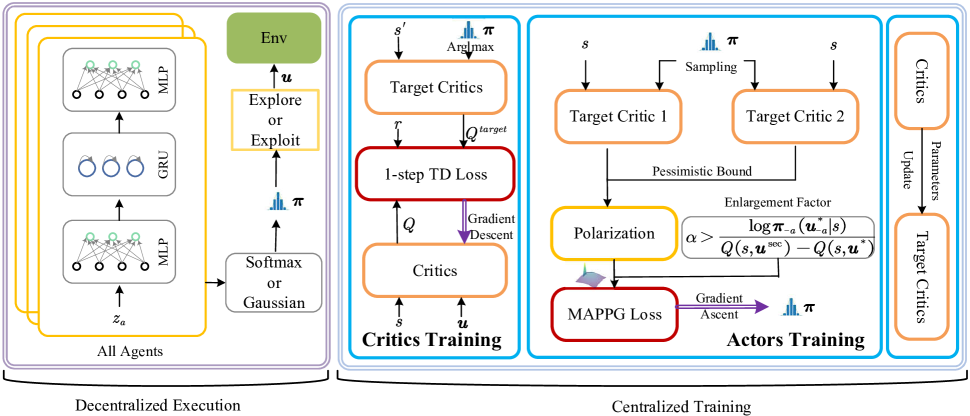
Figure 1: MAPPG framework.

Finally, we prove that optimal individual policies can be attained as long as MAPPG applies individual policy improvement to all agents in Theorem 2.

Theorem 2 (Joint Policy Improvement).

Let the joint action values remain unchanged during the policy improvement. Let $\boldsymbol{u}^{*}=\arg\max_{\boldsymbol{u}\in\boldsymbol{U}}Q(s,\boldsymbol{u})$ and $\boldsymbol{u}^{sec}=\arg\max_{\boldsymbol{u}\in(\boldsymbol{U}-\{\boldsymbol{u}^{*}\})}Q(s,\boldsymbol{u})$. Let the joint policy at iteration t be $\boldsymbol{\pi}^{t}=[\pi_{a}^{t}]_{a=1}^{n}$. If individual policy improvement is applied to each agent $a\in A$ and $\alpha>\max_{a\in A}\frac{\log\boldsymbol{\pi}^{0}_{-a}\left(\boldsymbol{u}_{-a}^{*}|s\right)}{Q\left(s,\boldsymbol{u}^{\sec}\right)-Q\left(s,\boldsymbol{u}^{*}\right)}$, then we have that $\boldsymbol{\pi}^{t}\rightarrow\boldsymbol{\pi}^{*}$ as $t\rightarrow\infty$, where $\arg\max_{\boldsymbol{u}}\boldsymbol{\pi}^{*}(\boldsymbol{u}|s)=\arg\max_{\boldsymbol{u}}Q\left(s,\boldsymbol{u}\right)$ .

Proof.

See Appendix B. ∎

Although Theorem 2 requires that when optimizing the policy of a single agent, other agents’ policies should be maintained as $\boldsymbol{\pi}_{-a}^{0}$. MAPPG replaces $\boldsymbol{\pi}_{-a}^{0}$ with the current policies $\boldsymbol{\pi}_{-a}^{t}$ of other agents in practice, which is a more efficient sampling strategy. This change does not compromise optimality empirically.

MAPPG Architecture

The overall framework of MAPPG is illustrated in Figure 1. For each agent $a$, there is an individual actor $\pi_{a}(u_{a}|\tau_{a})$ parameterized by $\theta_{a}$. We denote the joint policy as $\boldsymbol{\pi}=[\pi_{a}]_{a=1}^{n}$. Two centralized components are critics $Q(s,\boldsymbol{u})$ and target critics $Q^{target}(s,\boldsymbol{u})$, parameterized by $\phi$ and $\phi^{-}$.

At the execution phase, each agent selects actions w.r.t. the current policy and exploration based on the local observation in a decentralized manner. By interacting with the environment, the transition tuple $e=\left(s,[z_{a}]_{a=1}^{n},\boldsymbol{u},r,s^{\prime},[z_{a}^{\prime}]_{a=1}^{n}\right)$ is added to the buffer.

At the training phase, mini-batches of experiences are sampled from the buffer uniformly at random. We train the parameters of critics to minimise the 1-step TD loss by descending their gradients according to:

$$\nabla_{\phi}L_{td}\left(\phi\right)=\nabla_{\phi}\mathbb{E}_{e\sim D}\left[\left(y-Q\left(s,\boldsymbol{u}\right)\right)^{2}\right],$$ (7)

where $y=r+\gamma Q^{target}\left(s^{\prime},{\arg\max}_{\boldsymbol{u}^{\prime}}\ \boldsymbol{\pi}\left(\boldsymbol{u}^{\prime}|\tau^{\prime}\right)\right)$. In the proof of Theorem 2, some strong constraints need to be satisfied. To derive a practical algorithm, we must make approximations. First, MAPPG adopts target critics for individual policy improvement as an implementation of fixed joint action values. Second, the estimation of the Q-value has aleatoric uncertainty and epistemic uncertainty. Without a constraint, maximization of $J(\boldsymbol{\pi})$ with polarization would lead to an excessively large policy update; hence, we now consider how to modify the objective. We apply the pessimistic bound of $Q^{PPG}$ with the help of two target critics $\{Q_{1}^{target},\ Q_{2}^{target}\}$ and penalize changes to the policy that make $Q^{PPG}$ larger than $L$. We train two critics, which are learned with the same training setting except for the initialization parameters. The two target critics share the same network structure as that of the two critics, and the parameters of the two target critics are periodically synchronized with those of the two critics, respectively. We train the parameters of actors to maximize the expected polarization Q-function which is called the MAPPG loss by ascending their gradients according to:

$$\nabla_{\theta}J\left(\boldsymbol{\pi}\right)= \frac{1}{\beta}\mathbb{E}_{\boldsymbol{\pi}}\left[\sum_{a}{\nabla_{\theta_{a}}\log\pi_{a}\left(u_{a}\mid\tau_{a}\right)}\right.$$

$$\left.\min\left(\hat{Q}^{PPG}\left(s,\boldsymbol{u}\right),\,\,L\right)\right],$$ (8)

where

$$\hat{Q}^{PPG}(s,\boldsymbol{u})= \exp\left(\alpha\left(\min_{k\in\left\{1,2\right\}}Q_{k}^{target}\left(s,\boldsymbol{u}\right)\right.\right.$$

$$\left.\left.-\max_{k\in\left\{1,2\right\}}Q_{k}^{target}\left(s,\boldsymbol{u}_{curr}\right)\right)\right).$$

To prevent vanishing gradients caused by the increasing action probability with an inappropriate learning rate in practice, the gradients for the joint action $\boldsymbol{u}$ are set to 0 if $\hat{Q}^{PPG}(s,\boldsymbol{u})<1$ or $\forall a,\pi_{a}(u_{a}|\tau_{a})>P$ where $P\geq 0.5$, which is called the policy gradient clipping. For completeness, we summarize the training of MAPPG in the Algorithm 1. More details are included in Appendix C.

Algorithm 1 MAPPG

1:  for ${episode}=1$ to ${max\_training\_episode}$ do

2:     Initialize the environment

3:     for $t=1$ to $max\_episode\_length$ do

4:        For all agents, get the current state $s$ and observations $[z_{a}]_{a=1}^{n}$, choose a joint action $\boldsymbol{u}$ w.r.t. the current policy and exploration

5:        Execute the joint action $\boldsymbol{u}$, observe a reward $r$, and get the next state $s^{\prime}$ and observations $[z_{a}^{\prime}]_{a=1}^{n}$

6:        Add the transition $\left(s,[z_{a}]_{a=1}^{n},\boldsymbol{u},r,s^{\prime},[z_{a}^{\prime}]_{a=1}^{n}\right)$ to the buffer $D$

7:        if $time\_to\_update\_actors\_and\_critics$ then

8:           Sample a random minibatch of $K$ samples from $D$

9:           Update $\phi$ by descending their gradients according to Equation (7)

10:           Update $\theta$ by ascending their gradients according to Equation (8) with the policy gradient clipping

11:        end if

12:        if $time\_to\_update\_target\_critics$ then

13:           Replace target parameters $\phi_{i}^{-}\leftarrow\phi_{i}$ for $i\in\{1,2\}$

14:        end if

15:     end for

16:  end for

6 Experiments

In this section, first, we empirically study the optimality of MAPPG for discrete and continuous action spaces. Then, in StarCraft II, we demonstrate that MAPPG outperforms state-of-the-art MAPG algorithms. By ablation studies, we verify the effectiveness of our polarization joint action values and the pessimistic bound of $Q^{PPG}$. We further perform an ablation study to verify the effect of different enlargement factors on convergence to the optimum. In matrix and differential games, the worst result in the five training runs with different random seeds is selected to exclude the influence of random initialization parameters of the neural network. All the learning curves are plotted based on five training runs with different random seeds using mean and standard deviation in StarCraft II and the ablation experiment.

Matrix Game and Differential Game

In the discrete matrix and continuous differential games, we investigate whether MAPPG can converge to optimal compared with existing MAPG algorithms, including MADDPG (Lowe et al. 2017), COMA (Foerster et al. 2018), DOP (Wang et al. 2021b), FACMAC (Peng et al. 2021), and FOP (Zhang et al. 2021). The two games have one common characteristic: some destructive penalties are around with the optimal solution (Zhang et al. 2021), which triggers the issue of the centralized-decentralized mismatch.

	A	B	C
A	15	-12	-12
B	-12	10	10
C	-12	10	10

(a) Payoff of matrix game

	0.0(A)	0.8(B)	0.2(C)
0.0(A)	14.9	-11.8	-11.8
0.7(B)	-12.1	9.9	9.9
0.3(C)	-12.0	9.9	9.9

(b) COMA: $\pi_{1},\pi_{2},Q$

	0.0(A)	0.7(B)	0.3(C)
0.0(A)	-32.5	-11.2	-11.2
0.9(B)	-11.4	9.9	9.9
0.1(C)	-11.5	9.9	9.9

(c) DOP: $\pi_{1},\pi_{2},Q$

	0.0(A)	0.5(B)	0.5(C)
0.0(A)	-11.5	-11.5	-11.5
0.5(B)	-11.5	9.9	9.9
0.5(C)	-11.5	9.9	10.0

(d) FACMAC: $\pi_{1},\pi_{2},Q$

	0.0(A)	0.0(B)	1.0(C)
0.0(A)	9.1	-4.4	-7.4
0.0(B)	-5.3	9.0	5.0
1.0(C)	-2.6	9.0	9.7

(e) FOP: $\pi_{1},\pi_{2},Q$

	0.4(A)	0.3(B)	0.3(C)
0.4(A)	15.2	-12.2	-12.2
0.3(B)	-12.0	10.0	10.0
0.3(C)	-12.0	10.0	10.0

(f) MAPPG: $\pi_{1},\pi_{2},Q$

Table 1: The cooperative matrix game. Boldface means the optimal/greedy actions from individual policies.

Matrix Game

The matrix game is shown in Table 1 (a), which is the modified matrix game proposed by QTRAN (Son et al. 2019). This matrix game captures a cooperative multi-agent task where we have two agents with three actions each. We show the results of COMA, DOP, FACMAC, FOP, and MAPPG over 10$k$ steps, as in Table 1 (b) to 1 (f). MAPPG uses an $\epsilon$-greedy policy where $\epsilon$ is annealed from 1 to 0.05 over 10$k$ steps. MAPPG is the only algorithm that can successfully converge to the optimum. The results of these algorithms on the original matrix game proposed by QTRAN (Son et al. 2019), and more experiments and details are included in Appendix C.

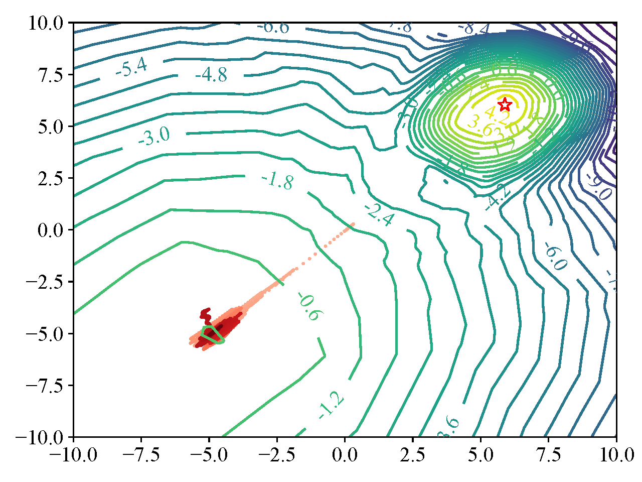
(a) MADDPG

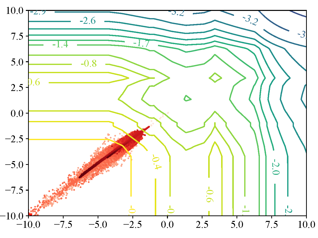
(b) FACMAC

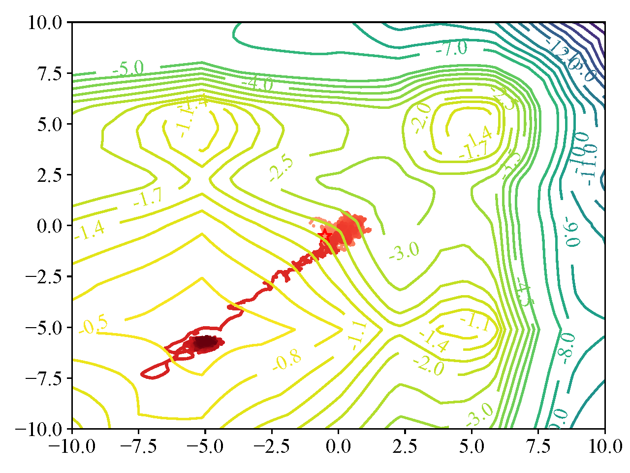
(c) FOP

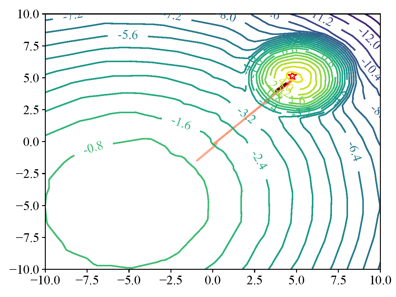
(d) MAPPG

Figure 2: Learning paths of different algorithms in the MTQ game. The horizontal and vertical axes represent $u_{1}$ and $u_{2}$, respectively. All the points on a given contour line are all at the same joint action values. The shallow red and dark red indicate the start and end of the learning paths, respectively.

Differential Game

The differential game is the modification of the Max of Two Quadratic (MTQ) Game from previous literature (Zhang et al. 2021). This is a single-state continuous game for two agents, and each agent has a one-dimensional bounded continuous action space ([-10, 10]) with a shared reward function. In Equation (12), $u_{1}$ and $u_{2}$ are the actions of two agents and $r(u_{1},u_{2})$ is the shared reward function received by two agents. There is a sub-optimal solution 0 at (-5, -5) and a global optimal solution 5 at (5, 5).

$$\left\{\begin{array}[]{l}f_{1}=0.8\times\left[-\left(\frac{u_{1}+5}{5}\right)^{2}-\left(\frac{u_{2}+5}{5}\right)^{2}\right]\\ f_{2}=1\times\left[-\left(\frac{u_{1}-5}{1}\right)^{2}-\left(\frac{u_{2}-5}{1}\right)^{2}\right]+5\\ r\left(u_{1},u_{2}\right)=\max\left(f_{1},f_{2}\right)\\ \end{array}\right..$$ (12)

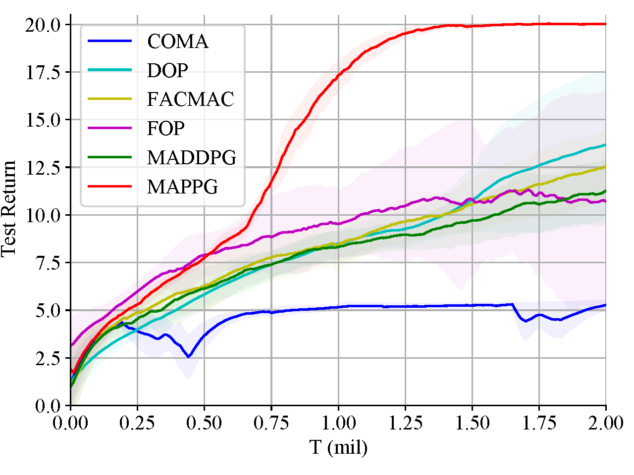
(a) 3s_vs_4z

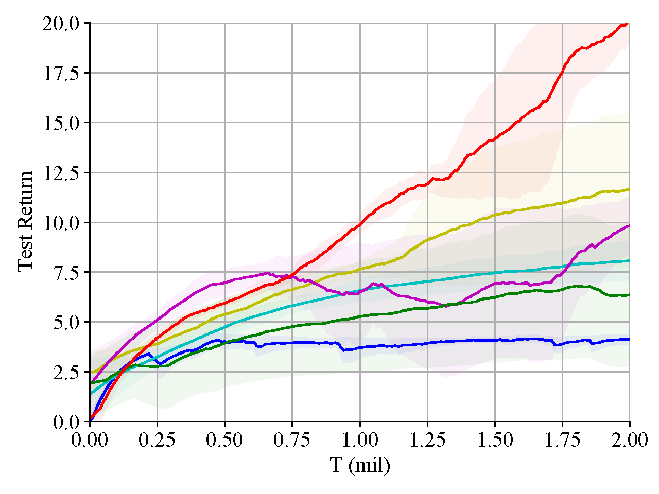
(b) 3s_vs_5z

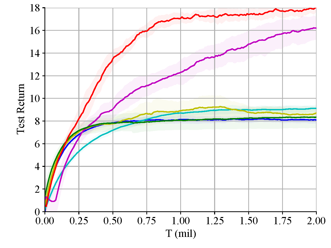
(c) 5m_vs_6m

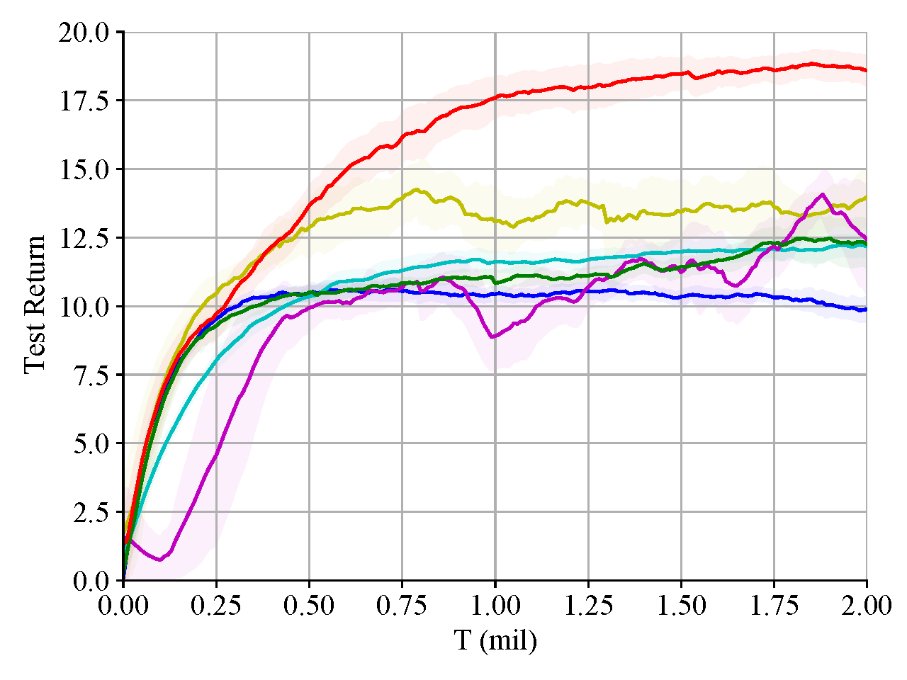
(d) 8m_vs_9m

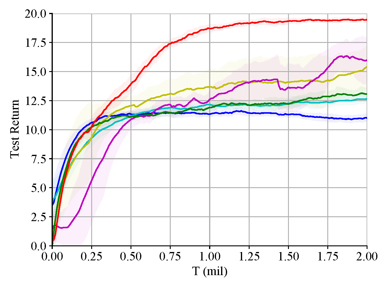
(e) 10m_vs_11m

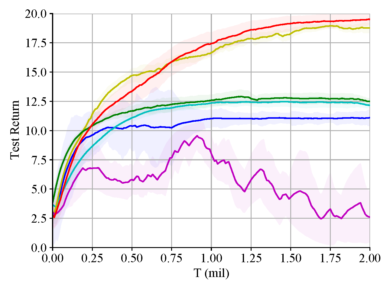
(f) 27m_vs_30m

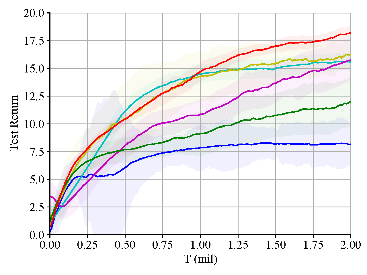
(g) MMM2

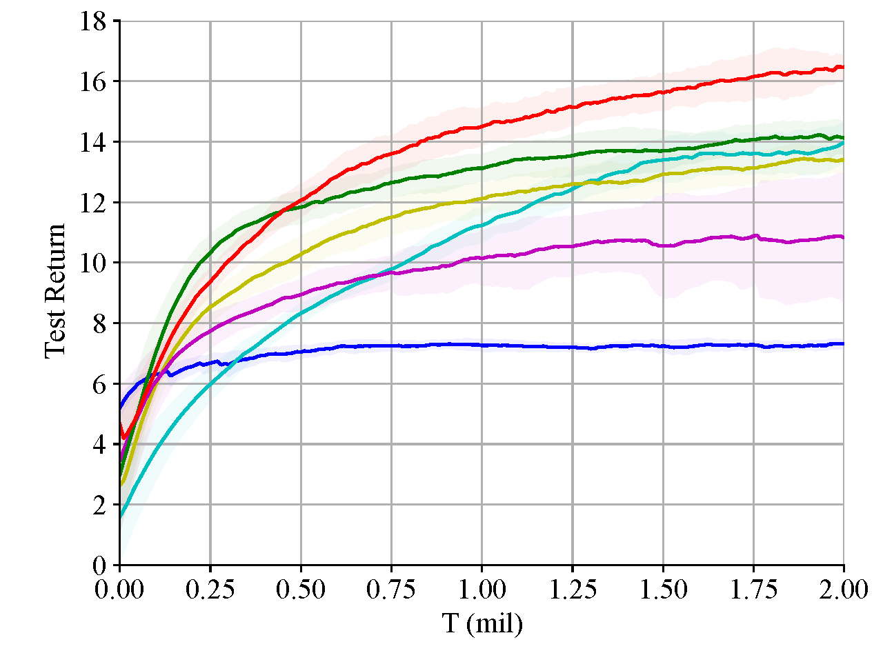
(h) 3s5z_vs_3s6z

Figure 3: Learning curves of all algorithms in eight maps of StarCraft II.

In MTQ, we compare MAPPG against existing multi-agent policy gradient algorithms, i.e., MADDPG, FACMAC, and FOP. Gaussian is used as the action distribution by MAPPG as in SAC (Haarnoja et al. 2018), and the mean of the Gaussian distribution is plotted. MAPPG uses a similar exploration strategy as in FACMAC, where actions are sampled from a uniform random distribution over valid actions up to 10$k$ steps and then from the learned action distribution with Gaussian noise. We use Gaussian noise with mean 0 and standard deviation 1. The learning paths (20$k$ steps) of all algorithms are shown as red dots in Figure 2 (a) to 2 (d). MAPPG consistently converges to the global optimum while all other baselines fall into the sub-optimum. MADDPG can estimate $r(u_{1},u_{2})$ accurately, but fail to converge to the global optimum. However, the regular decomposed actor-critic algorithms (FACMAC and FOP) converge to the sub-optimum and also have limitations to express $r(u_{1},u_{2})$. The results of these algorithms for the original MTQ game used by previous literature (Zhang et al. 2021), and more details are included in Appendix C.

StarCraft II

We evaluate MAPPG on the challenging StarCraft Multi-Agent Challenge (SMAC) benchmark (Samvelyan et al. 2019) in eight maps, including 3s_vs_4z, 3s_vs_5z, 5m_vs_6m, 8m_vs_9m, 10m_vs_11m, 27m_vs_30m, MMM2 and 3s5z_vs_3s6z. The baselines include 5 state-of-the-art MAPG algorithms (COMA, MADDPG, stochastic DOP, FOP, FACMAC). MAPPG uses an $\epsilon$-greedy policy in which $\epsilon$ is annealed from 1 to 0.05 over 50$k$ steps. Results are shown in Figure 3 and MAPPG outperforms all the baselines in the final performance, which indicates that MAPPG can jump out of sub-optima. More details of the StarCraft II experiments are included in Appendix C.

Ablation Studies

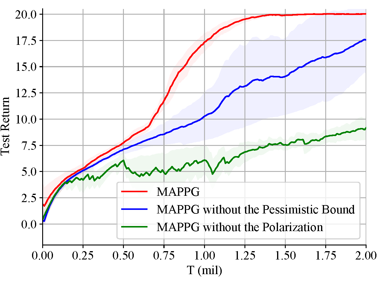
(a) 3s_vs_4z

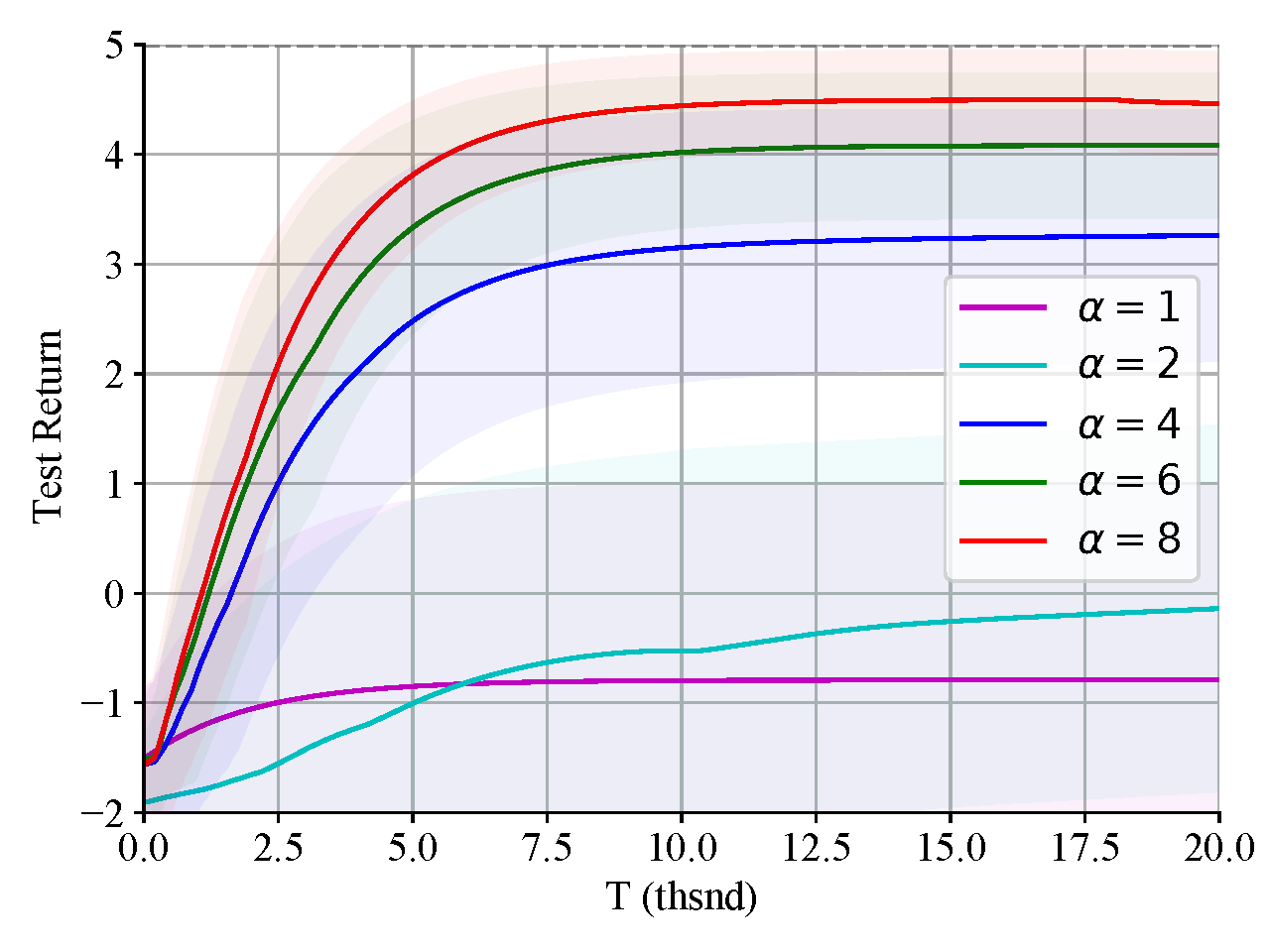
(b) MTQ

Figure 4: Ablations on the SMAC benchmark and MTQ game.

In Figure 4 (a), the comparison between the MAPPG and MAPPG without the pessimistic bound demonstrates the importance of making conservative policy improvements, which can alleviate the problem of excessively large policy updates caused by inaccurate value function estimation. The comparison between the MAPPG and MAPPG without the polarization demonstrates the contribution of polarization joint action values to global convergence. In Figure 4 (b), we observe that MAPPG can converge to a policy that can obtain a reward closer to the optimal reward as the increase of the enlargement factor. The discrepancy between the learning curve of $\alpha=\{1,\ 2\}$ and other learning curves indicates the influence of polarization. The difference in performance of different $\alpha$ is consistent with Theorem 1 and 2 even in the continuous action space.

7 Conclusion

This paper presents MAPPG, a novel multi-agent actor-critic framework that allows centralized end-to-end training and efficiently learns to do credit assignment properly to enable decentralized execution. MAPPG takes advantage of the polarization joint action value that efficiently guarantees the consistency between individual optimal actions and the joint optimal action. Our theoretical analysis shows that MAPPG can converge to optimality. Empirically, MAPPG achieves competitive results compared with state-of-the-art MAPG baselines for large-scale complex multi-agent cooperations.

References

- Agarwal et al. (2021) Agarwal, A.; Kakade, S. M.; Lee, J. D.; and Mahajan, G. 2021. On the Theory of Policy Gradient Methods: Optimality, Approximation, and Distribution Shift. Journal of Machine Learning Research, 22(98): 1–76.
- Balasubramanian et al. (2021) Balasubramanian, V.; Kobyzev, I.; Bahuleyan, H.; Shapiro, I.; and Vechtomova, O. 2021. Polarized-VAE: Proximity Based Disentangled Representation Learning for Text Generation. In Conference of the European Chapter of the Association for Computational Linguistics (EACL), 416–423.
- Cao et al. (2021) Cao, J.; Wang, X.; Darrell, T.; and Yu, F. 2021. Instance-Aware Predictive Navigation in Multi-Agent Environments. In IEEE International Conference on Robotics and Automation (ICRA), 5096–5102.
- Foerster et al. (2018) Foerster, J. N.; Farquhar, G.; Afouras, T.; Nardelli, N.; and Whiteson, S. 2018. Counterfactual Multi-Agent Policy Gradients. In AAAI Conference on Artifcial Intelligence (AAAI), 2974–2982.
- Goodfellow, Bengio, and Courville (2016) Goodfellow, I.; Bengio, Y.; and Courville, A. 2016. Deep Learning. MIT Press. http://www.deeplearningbook.org.
- Haarnoja et al. (2018) Haarnoja, T.; Zhou, A.; Abbeel, P.; and Levine, S. 2018. Soft Actor-Critic: Off-Policy Maximum Entropy Deep Reinforcement Learning with a Stochastic Actor. In International Conference on Machine Learning (ICML), 1856–1865.
- Hernandez-Leal, Kartal, and Taylor (2019) Hernandez-Leal, P.; Kartal, B.; and Taylor, M. E. 2019. A survey and critique of multiagent deep reinforcement learning. Autonomous Agents and Multi-Agent Systems, 33(6): 750–797.
- Konda and Tsitsiklis (1999) Konda, V. R.; and Tsitsiklis, J. N. 1999. Actor-Critic Algorithms. In Advances in Neural Information Processing Systems (NeurIPS), 1008–1014.
- Kraemer and Banerjee (2016) Kraemer, L.; and Banerjee, B. 2016. Multi-agent reinforcement learning as a rehearsal for decentralized planning. Neurocomputing, 190: 82–94.
- Lowe et al. (2017) Lowe, R.; Wu, Y.; Tamar, A.; Harb, J.; Abbeel, P.; and Mordatch, I. 2017. Multi-Agent Actor-Critic for Mixed Cooperative-Competitive Environments. In Advances in Neural Information Processing Systems (NeurIPS), 6379–6390.
- Oliehoek, Spaan, and Vlassis (2008) Oliehoek, F. A.; Spaan, M. T. J.; and Vlassis, N. 2008. Optimal and Approximate Q-value Functions for Decentralized POMDPs. Journal of Artificial Intelligence Research, 32: 289–353.
- Omidshafiei et al. (2017) Omidshafiei, S.; Pazis, J.; Amato, C.; How, J. P.; and Vian, J. 2017. Deep Decentralized Multi-task Multi-Agent Reinforcement Learning under Partial Observability. In International Conference on Machine Learning (ICML), 2681–2690.
- Peng et al. (2021) Peng, B.; Rashid, T.; de Witt, C. S.; Kamienny, P.; Torr, P. H. S.; Boehmer, W.; and Whiteson, S. 2021. FACMAC: Factored Multi-Agent Centralised Policy Gradients. In Advances in Neural Information Processing Systems (NeurIPS), 12208–12221.
- Proper and Tumer (2012) Proper, S.; and Tumer, K. 2012. Modeling difference rewards for multiagent learning. In International Conference on Autonomous Agents and Multiagent Systems (AAMAS), 1397–1398.
- Rashid et al. (2020) Rashid, T.; Farquhar, G.; Peng, B.; and Whiteson, S. 2020. Weighted QMIX: Expanding Monotonic Value Function Factorisation for Deep Multi-Agent Reinforcement Learning. In Advances in Neural Information Processing Systems (NeurIPS), 10199–10210.
- Rashid et al. (2018) Rashid, T.; Samvelyan, M.; Schroeder, C.; Farquhar, G.; Foerster, J.; and Whiteson, S. 2018. QMIX: Monotonic Value Function Factorisation for Deep Multi-Agent Reinforcement Learning. In International Conference on Machine Learning (ICML), 4295–4304.
- Samvelyan et al. (2019) Samvelyan, M.; Rashid, T.; de Witt, C. S.; Farquhar, G.; Nardelli, N.; Rudner, T. G. J.; Hung, C.; Torr, P. H. S.; Foerster, J. N.; and Whiteson, S. 2019. The StarCraft Multi-Agent Challenge. In International Conference on Autonomous Agents and Multiagent Systems (AAMAS), 2186–2188.
- Schulman et al. (2016) Schulman, J.; Moritz, P.; Levine, S.; Jordan, M. I.; and Abbeel, P. 2016. High-Dimensional Continuous Control Using Generalized Advantage Estimation. In International Conference on Learning Representations (ICLR).
- Shibata, Jimbo, and Matsubara (2021) Shibata, K.; Jimbo, T.; and Matsubara, T. 2021. Deep reinforcement learning of event-triggered communication and control for multi-agent cooperative transport. In IEEE International Conference on Robotics and Automation (ICRA), 8671–8677.
- Son et al. (2019) Son, K.; Kim, D.; Kang, W. J.; Hostallero, D.; and Yi, Y. 2019. QTRAN: Learning to Factorize with Transformation for Cooperative Multi-Agent Reinforcement Learning. In International Conference on Machine Learning (ICML), 5887–5896.
- Su, Adams, and Beling (2021) Su, J.; Adams, S. C.; and Beling, P. A. 2021. Value-Decomposition Multi-Agent Actor-Critics. In AAAI Conference on Artifcial Intelligence (AAAI), 11352–11360.
- Sunehag et al. (2018) Sunehag, P.; Lever, G.; Gruslys, A.; Czarnecki, W. M.; Zambaldi, V. F.; Jaderberg, M.; Lanctot, M.; Sonnerat, N.; Leibo, J. Z.; Tuyls, K.; and Graepel, T. 2018. Value-Decomposition Networks For Cooperative Multi-Agent Learning Based On Team Reward. In International Conference on Autonomous Agents and Multiagent Systems (AAMAS), 2085–2087.
- Sutton et al. (1999) Sutton, R. S.; McAllester, D. A.; Singh, S.; and Mansour, Y. 1999. Policy Gradient Methods for Reinforcement Learning with Function Approximation. In Advances in Neural Information Processing Systems (NeurIPS), 1057–1063.
- Wang et al. (2021a) Wang, J.; Ren, Z.; Liu, T.; Yu, Y.; and Zhang, C. 2021a. QPLEX: Duplex Dueling Multi-Agent Q-Learning. In International Conference on Learning Representations (ICLR).
- Wang et al. (2020) Wang, J.; Zhang, Y.; Kim, T.; and Gu, Y. 2020. Shapley Q-Value: A Local Reward Approach to Solve Global Reward Games. In AAAI Conference on Artifcial Intelligence (AAAI), 7285–7292.
- Wang et al. (2021b) Wang, Y.; Han, B.; Wang, T.; Dong, H.; and Zhang, C. 2021b. DOP: Off-Policy Multi-Agent Decomposed Policy Gradients. In International Conference on Learning Representations (ICLR).
- Wei and Luke (2016) Wei, E.; and Luke, S. 2016. Lenient Learning in Independent-Learner Stochastic Cooperative Games. Journal of Machine Learning Research, 17(84): 1–42.
- Wei et al. (2018) Wei, E.; Wicke, D.; Freelan, D.; and Luke, S. 2018. Multiagent Soft Q-Learning. In AAAI Spring Symposium Series.
- Zhang et al. (2021) Zhang, T.; Li, Y.; Wang, C.; Xie, G.; and Lu, Z. 2021. FOP: Factorizing Optimal Joint Policy of Maximum-Entropy Multi-Agent Reinforcement Learning. In International Conference on Machine Learning (ICML), 12491–12500.
- Zhou et al. (2020) Zhou, M.; Liu, Z.; Sui, P.; Li, Y.; and Chung, Y. Y. 2020. Learning Implicit Credit Assignment for Cooperative Multi-Agent Reinforcement Learning. In Advances in Neural Information Processing Systems (NeurIPS), 11853–11864.