CASAPose: Class-Adaptive and Semantic-
Aware Multi-Object Pose Estimation

Abstract

Applications in the field of augmented reality or robotics often require joint localisation and 6D pose estimation of multiple objects. However, most algorithms need one network per object class to be trained in order to provide the best results. Analysing all visible objects demands multiple inferences, which is memory and time-consuming. We present a new single-stage architecture called CASAPose that determines 2D-3D correspondences for pose estimation of multiple different objects in RGB images in one pass. It is fast and memory efficient, and achieves high accuracy for multiple objects by exploiting the output of a semantic segmentation decoder as control input to a keypoint recognition decoder via local class-adaptive normalisation. Our new differentiable regression of keypoint locations significantly contributes to a faster closing of the domain gap between real test and synthetic training data. We apply segmentation-aware convolutions and upsampling operations to increase the focus inside the object mask and to reduce mutual interference of occluding objects. For each inserted object, the network grows by only one output segmentation map and a negligible number of parameters. We outperform state-of-the-art approaches in challenging multi-object scenes with inter-object occlusion and synthetic training. Code is available at: https://github.com/fraunhoferhhi/casapose.

1 Introduction

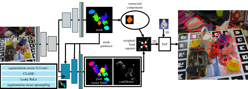
Figure 1: In CASAPose, a segmentation decoder estimates object masks that guide a second decoder to predict 2D-3D correspondences for single-stage multi-object pose estimation.

In this paper, we present CASAPose, a novel architecture specifically designed to improve multi-object scalability of a 6D pose estimator. Retrieving the pose of objects in front of a camera in real-time is essential for augmented reality and robotic object manipulation. Convolutional neural networks (CNN) led to a significant boost in accuracy and robustness against occlusion or varying illumination. Many methods train a separate CNN per object [Peng et al.(2019)Peng, Liu, Huang, Zhou, and Bao, Song et al.(2020)Song, Song, and Huang, Tremblay et al.(2018)Tremblay, To, Sundaralingam, Xiang, Fox, and Birchfield, Park et al.(2019a)Park, Patten, and Vincze, Li et al.(2019)Li, Wang, and Ji, Sundermeyer et al.(2018)Sundermeyer, Marton, Durner, Brucker, and Triebel]. In scenarios with multiple objects, this leads to impractical side effects. If it is not known which objects are present in the image, it must either be inspected individually for each known object or an additional detector is required for identification. Performing inference for each visible object increases the computation time. In addition, the need for multiple networks increases memory usage and lengthens training. Pose estimation is often formulated as an extension of semantic segmentation, with additional output maps to infer the pose from, e.g. 3D object coordinates, or keypoint locations encoded in vector fields. The trivial multi-object extension to expand this secondary output for each object [Peng et al.(2019)Peng, Liu, Huang, Zhou, and Bao] results in GPU-intensive slow training and performance degradation [Gard et al.(2022)Gard, Hilsmann, and Eisert].

Our approach decouples semantic object identification and keypoint regression and uses the pixel-wise segmentation results as guidance for a keypoint predicting branch. We introduce techniques from GAN-based conditional image synthesis and style transfer to the field of object pose estimation. First, we improve the descriptive capability of the network by adding a small amount of class specific extra weights to the network. Applying these parameters locally in the decoder as a class-adaptive de-(normalisation) (CLADE) [Tan et al.(2021)Tan, Chen, Chu, Chai, Liao, He, Yuan, Hua, and Yu] adds semantic awareness to the network. The locations of 3D keypoints on the object, represented by vectors pointing towards their 2D projection are interpreted as a local object-specific style. Second, we strengthen the local focus of the network by integrating two more semantic-aware operations [Dundar et al.(2020)Dundar, Sapra, Liu, Tao, and Catanzaro]. A guided convolution re-weights the convolutions in the keypoint branch and forces the decoder to focus on the mask region, when estimating the 6D pose. A segmentation-aware upsampling uses the mask during upscaling of feature maps to avoid misalignments between low-resolution features and high-resolution segmentation maps. Both operations reduce the interference between mutually occluding objects and improve the quality of the pose estimates. From the clearly separated output, the 2D-3D correspondences are localised in a robust and differentiable manner via weighted least squares. Since dataset creation for multi-object scenarios is very time consuming, we train only on synthetic data that comes with free labels and can be generated with free tools. To summarise, we make the following contributions:

1. We show that incorporating a small set of object-specific parameters through CLADE significantly increases the multi-object capacity of a pose estimation CNN.

2. We reduce the number of outputs of encoder-decoder based pose estimation networks and reduce intra-class interferences by segmentation-aware transformations.

3. We exploit the strictly local feature processing to obtain a new differentiable 2D keypoint estimation method improving the accuracy of 2D-3D correspondences.

4. We train our network only on synthetic images and achieve state-of-the art results on real data.

2 Related Work

Multi-Object 6D Pose Estimation

Approaches for 6D pose estimation with CNNs usually either regresses the object pose directly [Xiang et al.(2018)Xiang, Schmidt, Narayanan, and Fox, Billings and Johnson-Roberson(2019), Wang et al.(2020a)Wang, Manhardt, Shao, Ji, Navab, and Tombari], describe the object’s appearance with a latent space code to compare it to pre-generated codes [Sundermeyer et al.(2018)Sundermeyer, Marton, Durner, Brucker, and Triebel, Wen et al.(2020)Wen, Pan, Yang, and Wang, Park et al.(2020)Park, Mousavian, Xiang, and Fox], or regresses the position of 2D projections of 3D points and calculate the pose with a Perspective-n-Points (PnP) algorithm. Approaches from last category either predict object specific keypoints [Hu et al.(2019)Hu, Hugonot, Fua, and Salzmann, Peng et al.(2019)Peng, Liu, Huang, Zhou, and Bao, Song et al.(2020)Song, Song, and Huang, Tremblay et al.(2018)Tremblay, To, Sundaralingam, Xiang, Fox, and Birchfield, Rad and Lepetit(2017)] or dense correspondence/coordinate maps [Zakharov et al.(2019)Zakharov, Shugurov, and Ilic, Park et al.(2019a)Park, Patten, and Vincze, Hou et al.(2020)Hou, Ahmadyan, Zhang, Wei, and Grundmann, Thalhammer et al.(2021)Thalhammer, Leitner, Patten, and Vincze, Li et al.(2019)Li, Wang, and Ji, Hodan et al.(2020)Hodan, Barath, and Matas].

To deal with multiple objects, most approaches train a separate network per object and need multiple inferences per image [Peng et al.(2019)Peng, Liu, Huang, Zhou, and Bao, Song et al.(2020)Song, Song, and Huang, Tremblay et al.(2018)Tremblay, To, Sundaralingam, Xiang, Fox, and Birchfield, Park et al.(2019a)Park, Patten, and Vincze, Li et al.(2019)Li, Wang, and Ji, Sundermeyer et al.(2018)Sundermeyer, Marton, Durner, Brucker, and Triebel]. Alternatively, increasing the number of output maps is proposed as multi-object extension [Peng et al.(2019)Peng, Liu, Huang, Zhou, and Bao, Rad and Lepetit(2017), Hodan et al.(2020)Hodan, Barath, and Matas], which risks serious accuracy drops [Sock et al.(2020)Sock, Castro, Armagan, Garcia-Hernando, and Kim] or complex and slow processing [Hodan et al.(2020)Hodan, Barath, and Matas]. Each added object contributes multiple extra output channels having the same size as the input image, which requires significant GPU memory and complicates training [Gard et al.(2022)Gard, Hilsmann, and Eisert]. Sock et al[Sock et al.(2020)Sock, Castro, Armagan, Garcia-Hernando, and Kim] add additional weights to optimise a CNN for multiple objects and reduce the multi-object performance gap. Still, they need the object class as input from a separate bounding box detector to perform their re-parametrisation and one inference for every visible object. This principle is also applied by other multi-stage methods using object specific networks per detection [Li et al.(2019)Li, Wang, and Ji, Billings and Johnson-Roberson(2019), Park et al.(2019a)Park, Patten, and Vincze, Sundermeyer et al.(2018)Sundermeyer, Marton, Durner, Brucker, and Triebel, Zhang et al.(2021)Zhang, Zhao, Guan, Peng, and Peng, Yang et al.(2021)Yang, Yu, and Yang].

Other single-stage - multi-object strategies have rarely been discussed. The category level approach by Hou et al[Hou et al.(2020)Hou, Ahmadyan, Zhang, Wei, and Grundmann] unifies features from different instances of one class. It requires approximately similar geometric structure per category and aligned models during training. Similar to us, two recent works [Thalhammer et al.(2021)Thalhammer, Leitner, Patten, and Vincze, Aing et al.(2021)Aing, Lie, Chiang, and Lin] make single-stage multi-object pose estimation more performant by using a patch-based approach on a specialised feature pyramid network [Thalhammer et al.(2021)Thalhammer, Leitner, Patten, and Vincze], or by predicting an error mask to filter faulty pixels near silhouettes [Aing et al.(2021)Aing, Lie, Chiang, and Lin]. Especially for multi-object approaches, the use of synthetic training data is of high importance due difficult creation of real datasets [Thalhammer et al.(2021)Thalhammer, Leitner, Patten, and Vincze, Hodan et al.(2020)Hodan, Barath, and Matas]. It offers difficulties due to the domain gap [Wang et al.(2020a)Wang, Manhardt, Shao, Ji, Navab, and Tombari, Yang et al.(2021)Yang, Yu, and Yang, Zhang et al.(2021)Zhang, Zhao, Guan, Peng, and Peng], which we narrow down by giving the network access to the silhouettes, a nearly domain invariant feature [Wen et al.(2020)Wen, Pan, Yang, and Wang, Billings and Johnson-Roberson(2019)].

Conditional Normalisation

Normalisation layers in CNNs speed-up the training and improve the accuracy [Ioffe and Szegedy(2015)]. A learnable affine transformation recentres and rescales the normalised features. In the unconditional case, the normalisation does not depend on external data [Ioffe and Szegedy(2015), Ulyanov et al.(2016)Ulyanov, Vedaldi, and Lempitsky]. Conditional Instance Normalisation (CIN) [Dumoulin et al.(2017)Dumoulin, Shlens, and Kudlur] increases the capacity of a CNN by learning multiple sets of normalisation parameters for different classes, e.g. for neural style transfer [Gatys et al.(2015)Gatys, Ecker, and Bethge]. Sock et alapply CIN on multi-object 6D pose estimation [Sock et al.(2020)Sock, Castro, Armagan, Garcia-Hernando, and Kim], but require object identity as input and handle only one identity at a time. Spatially-adaptive instance (de)normalisation (SPADE) [Park et al.(2019b)Park, Liu, Wang, and Zhu] uses per-pixel normalisation parameters depending on semantic segmentation and a pixel’s position. Tan et al[Tan et al.(2021)Tan, Chen, Chu, Chai, Liao, He, Yuan, Hua, and Yu] reduce computational and parameter overhead of SPADE by prioritising semantic over spatial awareness. In their class-adaptive instance (de)normalisation (CLADE), a guided sampling operation selects the set of de-normalisation parameters based on the semantic class of a pixel. Similar to [Gard et al.(2022)Gard, Hilsmann, and Eisert], we extend [Sock et al.(2020)Sock, Castro, Armagan, Garcia-Hernando, and Kim] by first estimating a semantic segmentation and then infusing the CIN parameters on a local per-pixel level with a CLADE layer in a single pass.

Content-aware Transformations

While the spatial invariance of convolutions is beneficial for most computer vision tasks, sometimes local awareness of a filter can be helpful. CoordConv [Liu et al.(2018c)Liu, Lehman, Molino, Such, Frank, Sergeev, and Yosinski] demonstrates the benefit of giving a filter access to its position. It has been used for panoptic segmentation [Sofiiuk et al.(2019)Sofiiuk, Barinova, and Konushin, Wang et al.(2020b)Wang, Kong, Shen, Jiang, and Li] and semantic image synthesis [Tan et al.(2021)Tan, Chen, Chu, Chai, Liao, He, Yuan, Hua, and Yu]. Other approaches use binary maps to mask out regions of the feature map, e.g. for inpainting, depth upsampling, or padding [Liu et al.(2018a)Liu, Reda, Shih, Wang, Tao, and Catanzaro, Uhrig et al.(2017)Uhrig, Schneider, Schneider, Franke, Brox, and Geiger, Liu et al.(2018b)Liu, Shih, Wang, Reda, Sapra, Yu, Tao, and Catanzaro]. Guided convolutions have been extended for non-binary annotations [Yu et al.(2019)Yu, Lin, Yang, Shen, Lu, and Huang] and adapted for multi-class image synthesis [Dundar et al.(2020)Dundar, Sapra, Liu, Tao, and Catanzaro]. Mazzini et al[Mazzini(2018)] point out that spatially invariant operations for feature-map upsampling fail to capture the semantic information required by dense prediction tasks. Guided operations make upsampling learnable [Wang et al.(2019)Wang, Chen, Xu, Liu, Loy, and Lin, Mazzini(2018)]. The content-aware upscaling by Dundar et al[Dundar et al.(2020)Dundar, Sapra, Liu, Tao, and Catanzaro] takes advantage of a higher resolution mask to keep features aligned with the instance segmentation. We apply guided convolution and upsampling [Dundar et al.(2020)Dundar, Sapra, Liu, Tao, and Catanzaro] in our segmentation-aware decoder to force the network to focus on the object region when inferring the keypoint locations. This strengthens the local influence of the CLADE parameters inside the respective segmented region.

3 Multi-Object Pose Estimation

CASAPose is an encoder-decoder structure with two decoders applied successively (Fig. 1). The first estimates a segmentation mask that guides the second in estimating vectors pointing to 2D projections of predefined 3D object keypoints [Peng et al.(2019)Peng, Liu, Huang, Zhou, and Bao]. For each pixel, the set of keypoints corresponds to its semantic label. The second decoder additionally outputs confidences from which we calculate the common intersection points with weighted least squares (LS). The differentiable operation allows direct optimisation of the intersection point in the loss function.

3.1 Object-adaptive Local Weights

The injection of object-specific weights is intended to enhance the capacity of a pose estimation network for multiple objects. The process is therefore divided into two subtasks. First, a semantic segmentation $m\in\mathbb{L}^{H\times W}$ is estimated to specify each pixel’s object class, out of a set $\mathbb{L}$ with ${N_{c}}$ class indices, in an image of size $H\times W$. Second, a semantic image synthesis, conditioned on the semantic segmentation, generates a set of vector fields specifying 2D-3D correspondences of object keypoints to calculate poses from.

After a convolution, a conditional normalisation layer normalises each channel $k$ out of $N_{k}$ channels of features $x$ with its mean $\mu_{k}$ and standard deviation $\sigma_{k}$. The result is modulated with a learned scale $\gamma_{k}$ and shift $\beta_{k}$ depending on a condition $l=1,\dots,N_{c}$.

$$x^{out}_{k}=\gamma^{l}_{k}\frac{x_{k}-\mu_{k}}{\sigma_{k}}+\beta^{l}_{k}$$ (1)

To reach semantic-awareness, we follow the idea of class-adaptive (de)normalisation (CLADE) [Tan et al.(2021)Tan, Chen, Chu, Chai, Liao, He, Yuan, Hua, and Yu] and make the modulation parameters $\gamma$ and $\beta$ functions of the input segmentation. Thereby, a set $\Gamma=(\gamma^{1}_{k},\dots\gamma^{N_{c}}_{k})$ of scale, and a set $B=(\beta^{1}_{k},\dots\beta^{N_{c}}_{k})$ of shift parameters is learned. The intermediate semantic segmentation is used by Guided Sampling [Tan et al.(2021)Tan, Chen, Chu, Chai, Liao, He, Yuan, Hua, and Yu] to convert the sets to dense modulation tensors. Corresponding to the segmentation map, the modulation tensors are filled with the respective parameters, as shown in Fig. 2(a).

Guided Sampling uses a discrete index to select a specific row from a matrix of de-normalisation parameters. The required $argmax$ operation over the estimated class probabilities sacrifices differentiability, required for end-to-end training. To keep it, we directly use the segmentation input $S=(s_{x,y,l})\in\mathbb{R}^{H\times W\times N_{c}},s\in(0,1)$. The parameter sets are the matrices $\Gamma=(\gamma_{l,k})\in\mathbb{R}^{N_{c}\times N_{k}}$ and $B=(\beta_{l,k})\in\mathbb{R}^{N_{c}\times N_{k}}$, and the dense modulation tensors are the scalar product over the last dimension of $S$ and the parameter matrices $\Gamma$ and $B$.

$$\bar{\gamma}_{x,y,k}=\sum_{l=0}^{N_{c}}s_{x,y,l}\gamma_{l,k},\quad\bar{\beta}_{x,y,k}=\sum_{l=0}^{N_{c}}s_{x,y,l}\beta_{l,k}$$ (2)

Since this operation should simulate a discrete selection, the predicted label $s_{x,y,l}$ must be either close to 1 or 0. The raw intermediate segmentation $\hat{S}=(\hat{s}_{x,y,l})$ is normalised with a softmax function scaled with a temperature parameter $\tau$ to push all but one value close to 0.

$$s_{x,y,l}=softmax(\tau\hat{s}_{x,y,l})$$ (3)

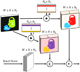
(a) CLADE using Guided Sampling.

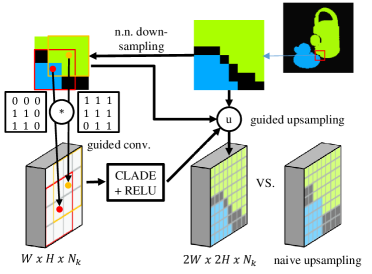
(b) Guided convolution and upsampling.

Figure 2: a) The segmentation is used to select modulation parameters from the weight matrices $\Gamma$ and $B$. b) Guided operations improve the alignment between features and mask.

3.2 Semantically Guided Decoder

Our goal is to synthesise keypoint vector fields, which are coherent and locally limited for each object. Based on the object a pixel belongs to, the vector should point to a particular location on that object. However, of course, occluding objects should not influence each other decreasing the accuracy in overlapping regions. We use pixel-wise object-specific weights to discriminate the objects from each other, and identify two challenges for the decoder.

1. Due to the spatial invariance of convolution, at object boundaries the decoder has no information which parameters were used to normalise a position in the previous block.

2. A nearest neighbour (NN) upsampling after CLADE does not result in a feature map that perfectly matches the higher resolution semantic map in the next block.

Inspired by Dundar et al[Dundar et al.(2020)Dundar, Sapra, Liu, Tao, and Catanzaro], we add segmentation-awareness to convolution and upsampling (Fig. 2(b)). The object-aware convolution ensures that the result of a convolution for an object only depends on feature values belonging to it. A mask $M$ filters weights $W$ for every image patch. The mask defines which locations contribute to the feature values and depends on the semantic segmentation $S$. To preserve differentiability, we avoid $argmax$ and do not use a hard binary mask.

$$m_{x,y}(i,j)=\begin{cases}\bar{s}_{x+i,y+j}&\parbox[t]{113.81102pt}{ \text{if} \quad$s_{x+i,y+j,l}=\bar{s}_{x+i,y+j}$ \text{with} \quad$\{l|s_{x,y,l}=\bar{s}_{x,y}\}$ }\\ 0&\text{otherwise}\end{cases}$$ (4)

In Equ. 4, $\bar{s}$ is the maximum value along the class dimension of $S$. The indices $x,y$ correspond to the filter location in the image, $i,j$ to the position in the filter. We apply the object-aware convolution with a $3\times 3$ filter at every location by element-wise multiplication of the input features $X$ with mask $M$ before filtering, followed by normalisation.

$$x^{\prime}=W^{T}(X\odot M)\frac{9}{sum(M)}$$ (5)

The object-aware upsampling layer enlarges the feature map without losing the alignment with $S$. Initially, $S$ is NN down-sampled $n$ times ($n=3$) to be used with features in different resolutions. The segmentation in the next higher and current resolution, $S^{u}$ and $S^{d}$, guide the upsampling from low to high resolution features, $F^{d}$ and $F^{u}$ [Dundar et al.(2020)Dundar, Sapra, Liu, Tao, and Catanzaro]. This preserves the spatial layout in the feature map after the object-aware convolution and CLADE. We do not apply hole-filling, and select the first feature in the $2\times 2$ windows for unknown locations.

3.3 Differentiable Keypoint Regression

The local processing of the latent map adds semantic-awareness to process different regions independently. We use this property to avoid the non-differentiable RANSAC estimation, commonly used to get 2D points from vector fields [Peng et al.(2019)Peng, Liu, Huang, Zhou, and Bao]. While exact intersection points can only be calculated for line pairs, a least squares solution can approximate them from multiple vectors [Traa(2013)]. Each vector inside a semantic region adds one equation to a corresponding linear system. Solving with the Moore-Penrose pseudoinverse guarantees a unique solution. An estimated per-pixel confidence captures the probability that a vector points in the right direction. Weighting equations with the estimated confidence reduces the susceptibility to noise [Traa(2013)]. An additional loss minimises the euclidian distance between the calculated 2D coordinate and ground truth. By this, the network learns in which regions the most accurate vectors are predicted and boosts their weighting in the calculation. We observe a focus on nearby regions as well as the object contour (Fig. 5). A custom layer calculates the intersection points in parallel on the GPU, so that the network outputs the 2D locations directly. The confidence maps increase the number of outputs by the number of keypoints per object.

During inference, we cluster the semantic maps in connected components and solve the system for the largest component per class. By this, potential misdetections in the semantic map can be filtered out. This works very well, if only one instance of each object is visible per image. For an extension to instance segmentation the semantic segmentation encoder would have to be replaced by an instance segmentation decoder, e.g. [Cheng et al.(2020)Cheng, Collins, Zhu, Liu, Huang, Adam, and Chen]. Since the components from Section 3.1 and 3.2 can also be applied to instance masks, all their advantages remain.

3.4 Merged Network Outputs

The object-specific weights in the CLADE layers serve as a key in the decoder to decipher the encoded weights in a characteristic manner. The local processing by the object-aware operations minimises performance degradation and crosstalk between objects. The loss function is applied on the fused output directly. The number of channels of the keypoint decoder is constant and only one channel is added per object in the segmentation decoder. For each keypoint, we compute a confidence map and a 2D vector field. This results in $3m+n+1$ output channels for $n$ objects with $m$ keypoints, e.g. $41$ for $13$ objects (and 9 keypoints), compared to $248$ outputs for PVNet [Peng et al.(2019)Peng, Liu, Huang, Zhou, and Bao] or $3342$ for EPOS [Hodan et al.(2020)Hodan, Barath, and Matas]. The constant number of outputs reduces the GPU memory footprint and quickens inference and training.

4 Implementation Details

Architecture

In CASAPose, a shared ResNet-18 [He et al.(2016)He, Zhang, Ren, and Sun, Peng et al.(2019)Peng, Liu, Huang, Zhou, and Bao] provides features for two decoders. The first resembles [Peng et al.(2019)Peng, Liu, Huang, Zhou, and Bao] and predicts a semantic mask by multiple blocks of consecutive skip connections, convolutions, batch normalisation (BN), leaky ReLU, and upsampling. The keypoint decoder is similar, but replaces BN with CLADE, the regular convolution with an object-aware convolution, and the blind upsampling with object-aware upsampling. Each block takes a scaled semantic mask as additional input to guide the replaced layers. We observed improved convergence if the ground truth segmentation instead of the output of the keypoint decoder is used for supervision. Both decoders can thereby calculate their result in parallel, which results in faster training. The semantic mask, the vector field, and the confidence maps are passed to a keypoint regressing layer (Section 3.3). It outputs 9 2D keypoints for each object. Their 3D locations were initially calculated using the farthest point sampling (FPS) algorithm. The pose is estimated with OpenCV’s EPnP [Lepetit et al.(2009)Lepetit, Moreno-Noguer, and Fua] in an RANSAC scheme. Due to its lightweight backbone our network is small and has only $\approx 14.8$ million weights. The CLADE layers increase the total number of weights by only 1024 per object.

Training Strategy

During training, all but one of the scenes from the Bop Challenge 2020 [Hodaň et al.(2020)Hodaň, Sundermeyer, Drost, Labbé, Brachmann, Michel, Rother, and Matas] synthetic LINEMOD dataset are used. The images are rendered nearly photo realistically with physically-based rendering (pbr). Object and scene parameters, e.g. object, camera and illumination position, background texture, and material are randomised. The objects are randomly placed on a flat surface with mutual occlusions. We narrow the domain gap by strong augmentation (contrast, colour, blur, noise). We follow Thalhammer et al[Thalhammer et al.(2021)Thalhammer, Leitner, Patten, and Vincze] but vary the gain for sigmoid contrast [Jung(2020)] to be $\mathcal{U}(5,10)$, since the listed values corrupt the image too much. Each network is trained for 100 epochs using the Adam optimiser [Kingma and Ba(2015)] and a batch size of 18 on two NVIDIA A100 GPUs (4 is the maximum for a single Nvidia RTX 2080Ti). The initial learning rate of $0.001$ is halved after 50, 75 and 90 epochs. We use smooth $\ell 1$ loss $\mathcal{L}_{Vec}$ and Differentiable Proxy Voting Loss (DPVL) [Yu et al.(2020)Yu, Zhuang, Koniusz, and Li] $\mathcal{L}_{PV}$ to learn the unit vectors, and Cross Entropy Loss with Softmax $\mathcal{L}_{Seg}$ the learn the segmentation. Additionally, the keypoint loss $\mathcal{L}_{Key}$ is defined as the smooth $\ell 1$ of the average Euclidean distance between the estimated keypoints and the ground truth keypoints. The overall loss is

$$\mathcal{L}=\lambda_{1}\mathcal{L}_{Seg}+\lambda_{2}\mathcal{L}_{Vec}+\lambda_{3}\mathcal{L}_{PV}+\lambda_{4}\mathcal{L}_{Key}$$ (6)

with $\lambda_{1}=1.0$ , $\lambda_{2}=0.5$, $\lambda_{3}=0.015$ and $\lambda_{4}=0.007$. The $\lambda$ values were determined in empirical preliminary studies using the unseen pbr scene.

5 Experiments

We use test images and objects from the widely used datasets LINEMOD (LM) [Hinterstoisser et al.(2012)Hinterstoisser, Lepetit, Ilic, Holzer, Bradski, Konolige, and Navab], Occluded LINEMOD (LM-O) [Brachmann et al.(2014)Brachmann, Krull, Michel, Gumhold, Shotton, and Rother], and HomebrewedDB (HB) [Kaskman et al.(2019)Kaskman, Zakharov, Shugurov, and Ilic]. We avoid real camera images in training because for practical applications capturing and annotation of large multi-object datasets is unrealistically costly. Our network estimates the poses of all detected objects in one pass. We report the standard metrics ADD and ADD-S [Xiang et al.(2018)Xiang, Schmidt, Narayanan, and Fox] for symmetric (glue and eggbox) objects, and the 2D projection [Hinterstoisser et al.(2012)Hinterstoisser, Lepetit, Ilic, Holzer, Bradski, Konolige, and Navab] (2DP) metric. For ADD/S, the average 3D distance (between ground truth (gt) and transformed vertices) must be smaller then 10% of the object diameter; for 2DP the 2D distance (between projected gt and transformed vertices) must be smaller than 5 pixel, for poses to be considered as correct. We always list the recall of correct poses per object. Additional results can be found in the Appendix.

5.1 Comparison with the State of the Art

Occluded LINEMOD (LM-O) [Brachmann et al.(2014)Brachmann, Krull, Michel, Gumhold, Shotton, and Rother]

Table 1 compares the ADD/S metric on LM-O against other papers which only train on synthetic data or use additional unlabelled images from the test domain [Li et al.(2021)Li, Hu, Salzmann, and Ji, Wang et al.(2020a)Wang, Manhardt, Shao, Ji, Navab, and Tombari, Yang et al.(2021)Yang, Yu, and Yang]. CASAPose achieves 27.8% better results than the other single-stage multi-object approach PyraPose [Thalhammer et al.(2021)Thalhammer, Leitner, Patten, and Vincze]. In contrast to their finding, favouring patch based approaches over encoder decoder networks, we show that it is possible to achieve better results with a considerably smaller encoder-decoder network. CASAPose performs 3.8% better than SD-Pose [Li et al.(2021)Li, Hu, Salzmann, and Ji], a state-of-the-art approach using entirely synthetic training data, but we only train a single network for all objects and omit pre-detection and preprocessing. DAKDN [Zhang et al.(2021)Zhang, Zhao, Guan, Peng, and Peng], the best weakly supervised approach is outperformed by 6.5%. Like us, the Top-2-6 approaches [Zhang et al.(2021)Zhang, Zhao, Guan, Peng, and Peng, Li et al.(2021)Li, Hu, Salzmann, and Ji, Thalhammer et al.(2021)Thalhammer, Leitner, Patten, and Vincze, Wang et al.(2020a)Wang, Manhardt, Shao, Ji, Navab, and Tombari, Yang et al.(2021)Yang, Yu, and Yang] all use physically-based rendered (pbr) images in training. Compared to approaches using simpler synthetic data, namely CDPN [Li et al.(2019)Li, Wang, and Ji] and DPOD [Zakharov et al.(2019)Zakharov, Shugurov, and Ilic] our algorithm achieves far superior results. The result for ’eggbox’ is weaker than for the other methods. Its symmetry leads to ambiguities of the 2D keypoint projections during training. Future work might consider adding a differentiable renderer and a projection, e.g. edge-based loss, to explicitly account for symmetry. In addition, ’eggbox’ is often heavily occluded, and inclusion of real images (e.g. semi-supervised) could improve its detection rate. For EPOS [Hodan et al.(2020)Hodan, Barath, and Matas], another single-stage approach, only the Average Recall (AR) [Hodaň et al.(2020)Hodaň, Sundermeyer, Drost, Labbé, Brachmann, Michel, Rother, and Matas] metric is listed with a value of 44.3, whereas our presented results correspond to an AR of 54.2..

LINEMOD (LM) [Hinterstoisser et al.(2012)Hinterstoisser, Lepetit, Ilic, Holzer, Bradski, Konolige, and Navab]

Table 2 compares our result on LM with one network trained for 13 objects to other methods using only synthetic training data. The achieved mean ADD/S of 68.1% is 1.2% better than SD-Pose [Li et al.(2021)Li, Hu, Salzmann, and Ji] and 7.4% better than PyraPose [Thalhammer et al.(2021)Thalhammer, Leitner, Patten, and Vincze].

HomebrewedDB (HB) [Kaskman et al.(2019)Kaskman, Zakharov, Shugurov, and Ilic]

The second sequence of HB is a benchmark to check whether a method generalises well to a novel domain [Kaskman et al.(2019)Kaskman, Zakharov, Shugurov, and Ilic]. It contains three objects from LM, captured with a different camera in a new environment. Our network trained for LM is used without retraining and the result far surpasses the next best method DAKDN [Zhang et al.(2021)Zhang, Zhao, Guan, Peng, and Peng] by 35% (Table 3). By focusing on the object mask and because 2D-3D correspondences are predicted instead of a full 6D pose, our method shows high invariance to new environments and different capture devices. To verify the latter, another version of the same sequence captured with Kinect (also part of HB) is checked. The camera parameters differ more, but the result is almost as good.

Method	Data	single-st.	Ape	Can	Cat	Drill	Duck	Eggb.	Glue	Hol.	Avg.
DPOD[Zakharov et al.(2019)Zakharov, Shugurov, and Ilic]	syn.	✓	2.3	4.0	1.2	10.5	7.2	4.4	12.9	7.5	6.3
CDPN[Li et al.(2019)Li, Wang, and Ji]	syn.	-	20.0	15.1	16.4	5.0	22.2	36.1	27.9	24.0	20.8
DSC-PoseNet[Yang et al.(2021)Yang, Yu, and Yang]	pbr+RGB	-	9.1	21.1	26.0	33.5	12.2	39.4	37.0	20.4	24.8
PyraPose[Thalhammer et al.(2021)Thalhammer, Leitner, Patten, and Vincze]	pbr	✓	18.5	46.4	11.7	48.2	19.4	16.7	30.7	33.0	28.1
Self6D[Wang et al.(2020a)Wang, Manhardt, Shao, Ji, Navab, and Tombari]	pbr+RGBD	-	13.7	43.2	18.7	32.5	14.4	57.8	52.3	22.0	32.1
DAKDN[Zhang et al.(2021)Zhang, Zhao, Guan, Peng, and Peng]	pbr+RGB	-	-	-	-	-	-	-	-	-	33.7
SD-Pose[Li et al.(2021)Li, Hu, Salzmann, and Ji]	pbr	-	21.5	56.7	17.0	44.4	27.6	42.8	45.2	21.6	34.6
CASAPose	pbr	✓	24.3	59.5	15.2	57.5	26.0	14.7	55.4	34.3	35.9

Table 1: Comparison of ADD/S-Recall with SoTA approaches on LM-O with synthetic only or weakly supervised training using unlabeled real data.

Method	Ape	Bv.	Cam	Can	Cat	Drill	Duck	Eggb.	Glue	Hol.	Iron	Lamp.	Ph.	Avg.
AAE [Sundermeyer et al.(2018)Sundermeyer, Marton, Durner, Brucker, and Triebel]	4.2	22.9	32.9	37.0	18.7	24.8	5.9	81.0	46.2	18.2	35.1	61.2	36.3	32.6
MHP[Manhardt et al.(2019)Manhardt, Arroyo, Rupprecht, Busam, Birdal, Navab, and Tombari]	11.9	66.2	22.4	59.8	26.9	44.6	8.3	55.7	54.6	15.5	60.8	-	34.4	38.8
Self6D-LB[Wang et al.(2020a)Wang, Manhardt, Shao, Ji, Navab, and Tombari]	37.2	66.9	17.9	50.4	33.7	47.4	18.3	64.8	59.9	5.2	68.0	35.3	36.5	40.1
DPOD[Zakharov et al.(2019)Zakharov, Shugurov, and Ilic]	35.1	59.4	15.5	48.8	28.1	59.3	25.6	51.2	34.6	17.7	84.7	45.0	20.9	40.5
PyraPose[Thalhammer et al.(2021)Thalhammer, Leitner, Patten, and Vincze]	22.8	78.6	56.2	81.9	56.2	70.2	40.4	84.4	82.4	42.6	86.4	62.0	59.5	63.4
SD-Pose[Li et al.(2021)Li, Hu, Salzmann, and Ji]	54.0	76.4	50.2	81.2	71.0	64.2	54.0	93.9	92.6	24.0	77.0	82.6	53.7	67.3
CASAPose	30.3	94.8	60.0	83.9	60.5	89.2	37.6	71.0	80.7	30.7	84.5	89.9	71.7	68.1

Table 2: Comparison of ADD/S-Recall with SoTA approaches on LM with synthetic training.

Method	DPOD[Zakharov et al.(2019)Zakharov, Shugurov, and Ilic]	PyraP.[Thalhammer et al.(2021)Thalhammer, Leitner, Patten, and Vincze]	DSC-P.[Yang et al.(2021)Yang, Yu, and Yang]	Self6D[Wang et al.(2020a)Wang, Manhardt, Shao, Ji, Navab, and Tombari]	DAKDN[Zhang et al.(2021)Zhang, Zhao, Guan, Peng, and Peng]	Ours	Ours‡
Avg.	32.7	41.3†	44.0	59.7†	63.8	86.3	84.4

Table 3: Comparison of ADD/S-Recall on HB. Methods indicated with (^†) retrain with data from the target domain. We list results for the Primesense and Kinect (^‡) sequence.

5.2 Ablation Study

Table 4 shows the effects of different components of our architecture. We train models for 13 objects and evaluate on LM, LM-O and the unseen pbr scene [Hodaň et al.(2020)Hodaň, Sundermeyer, Drost, Labbé, Brachmann, Michel, Rother, and Matas] to see improvements with and without domain gap. The simplest model (Base) uses the merged vector field, but otherwise resembles PVNet [Peng et al.(2019)Peng, Liu, Huang, Zhou, and Bao]. The model is gradually expanded to include the second decoder with CLADE (C) and the semantically guided operations (C/GCU). For each case, we train a network with and without confidence output, i.e. with Differentiable Keypoint Regression (DKR) or RANSAC based voting (RV). Averaged over the three datasets, adding C and C/GCU improves ADD/S by 13.6% and 17.9% compared to Base for the RV networks. This demonstrates that extended network capacity with C and the enforced local processing with GCU improve the quality of the estimated vector fields. Adding DKR further improves ADD/S by 16.1% for C and 17.6% for C/GCU, compared to the respective network with RV. The total improvement from Base with RV to the final network is 38.7% for ADD/S and 7.14% for 2DP. Adding DKR to Base also improved ADD/S by 24.5%, and 2DP by 4.3% showing that its ability to assign low confidences e.g. at overlapping regions improves already the simplest architecture. We notice that adding GCU to a network using DKR is especially effective for the datasets with domain gap and even more if occlusion is present (9.3% and 7.3% improvement over C+DKR compared to 2.7% improvement for pbr). The reason we give for this is that the contour is a cross-domain feature, and access to the silhouette and consequent higher weighting of nearby vectors helps bridging the domain gap. Fig. 5 shows this as well as the sharp separation of the vector fields at object boundaries due to C/GCU.

Arch.	without keypoint regression (RV)						with keypoint regression (DKR)
	LM-O		LM		pbr		LM-O		LM		pbr
	2DP	ADD/S	2DP	ADD/S	2DP	ADD/S	2DP	ADD/S	2DP	ADD/S	2DP	ADD/S
Base	45.3	22.2	90.0	49.8	74.6	42.2	49.4	28.9	91.7	59.2	77.9	52.5
C	47.3	26.6	91.8	55.7	76.5	47.5	51.4	29.9	93.6	64.7	79.3	56.1
C/GCU	49.2	26.7	91.4	59.0	77.3	49.0	51.5	32.7	93.8	68.1	79.6	57.6

Table 4: Ablation study: Comparison of different network architectures on different datasets.

5.3 Influence of the Object Number

The multi-object capacity of CASAPose with respect to the 2DP and ADD/S metric is evaluated in Table 5. Poses are estimated for the 8 LM-O objects on LM and LM-O. While the 8-object network on LM is about as good as the 13-object network, it performs 8% better on LM-O. Splitting the objects in two groups of four (ape-drill, duck-holepuncher) leads to a further increase of both metrics. The two-network solution increases ADD/S on LM-O to 38.7%, further extending the distance to the methods in Table 1. This increase can be partially explained by the exclusion of symmetrical objects from the first group for which we also observed a stronger enhancement. Future experiments might evaluate the use of a more recent segmentation backbone to further narrow down the observed multi-object gap.

5.4 Running Time

The runtime from image input to final poses for all visible objects in LM-O is 37.3 ms on average with the 8-object model. It splits in 18.8 ms for network inference, 1.7 ms for DKR, about 2.9 ms for PnP, and 13.9 ms for finding the largest connected-component (CC) for each class. This results in about 27 frames per second on our test GPU (Nvidia A100). We propose to replace the CC analysis with an instance centre prediction (e.g. like [Cheng et al.(2020)Cheng, Collins, Zhu, Liu, Huang, Adam, and Chen]) in future work to add instance awareness to our method and replace the cost intensive processing.

	LM-O		LM
	2DP	ADD/S	2DP	ADD/S
13 Obj.	51.5	32.7	96.0	60.4
8 Obj.	54.7	35.9	96.9	59.2
4 Obj. (2x)	58.4	38.7	97.3	64.5

Table 5: Influence of object number per network on ADD/S-Recall.

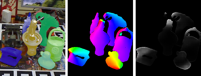
Figure 3: Estimated masks, colour coded vector fields, and confidence maps with C/GCU (f.l.t.r).

6 Conclusion

We showed that class-adaptiveness and semantic awareness improve the performance of a multi-object 6D pose estimator. Local feature processing minimises interference between overlapping regions in an reduced output space. Object-specific parameters selected via CLADE in a second decoder strengthen the prediction accuracy. The locality of the operations allows region-wise predictions, e.g. of least square weights, where we demonstrated a reduction of domain gap with our Differentiable Keypoint Regression. This also enables the direct addition of additional steps, such as pose refinement, in an end-to-end solution in future work. The presented layers are general enough to be integrated also in other pose estimation architectures.

Appendix

We provide visual results of CASAPose in Section A. Section B contains further comparisons with the state of the art as well as two more experiments. Finally, Section C lists additional implementation details.

Appendix A Visual Results

Fig. 4 shows estimated poses for three example images from Occluded LINEMOD (LM-O) [Brachmann et al.(2014)Brachmann, Krull, Michel, Gumhold, Shotton, and Rother] using CASAPose trained for 8 objects. Similarly, Fig. 5 gives an impression of example results using a model trained for 13 objects on our pbr test scene [Hodaň et al.(2020)Hodaň, Sundermeyer, Drost, Labbé, Brachmann, Michel, Rother, and Matas]. Example results of CASAPose for HomebrewedDB (HB) [Kaskman et al.(2019)Kaskman, Zakharov, Shugurov, and Ilic] are shown in Fig. 6.

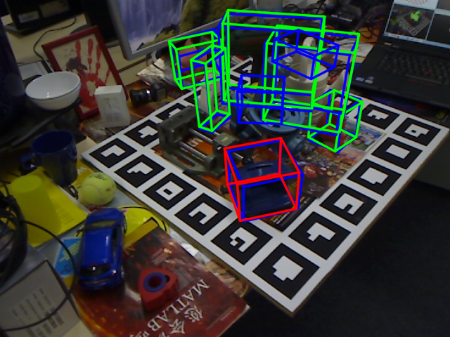
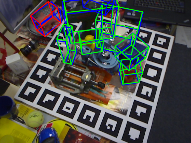
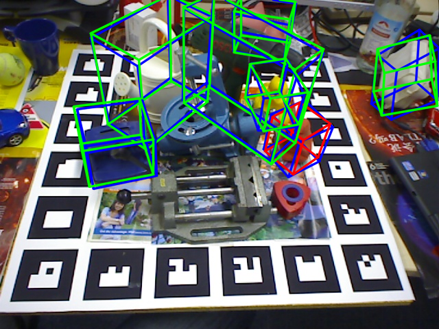
Figure 4: Example results of CASAPose for LM-O, with bounding boxes for correctly estimated poses in green, incorrect poses in red, and ground truth poses in blue (ADD/S metric).

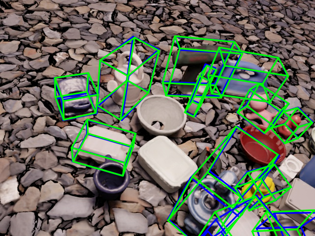
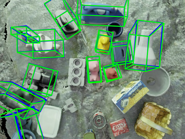
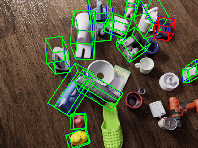
Figure 5: Example results of CASAPose for pbr images excluded during training, with bounding boxes for correctly estimated poses in green, incorrect poses in red, and ground truth poses in blue (ADD/S metric).

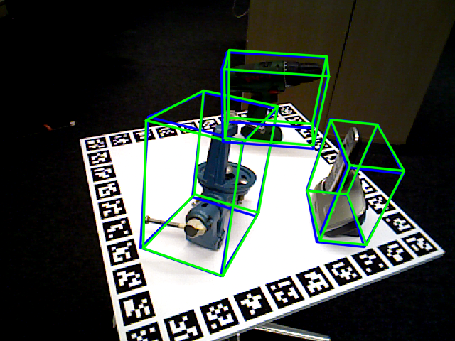
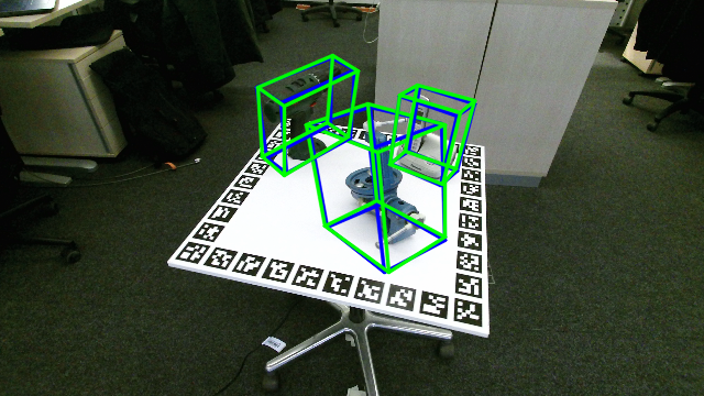
Figure 6: Example results of CASAPose for HB, with bounding boxes for correctly estimated poses in green and ground truth poses in blue (ADD/S metric). The left image is captured with the PrimeSense Carmine camera; the right image is captured with Microsoft Kinect 2.

A.1 Effect of Guided Operations

The ablation study discovered that semantic guidance improves the estimated vector fields and the accuracy of pose estimation. The effect is best seen in direct visual comparison. Fig. 7 shows the enhancement exemplified for an image from the pbr dataset using colour coded vector fields for visualisation. It shows the vector fields for the first keypoint, which is always located in the centre of each object. Comparing the output of a model without the guided decoder in Fig. 7(b) with the output of a model with object-aware convolutions and object-aware upsampling in Fig. 7(c), there is a clear improvement in vector fields, especially in regions where objects overlap. In fact, we have observed that a network without semantic guidance is not even able to produce perfectly separated vector fields when it heavily overfits only a few images. Using CLADE alone without semantic guidance already improves the quality of the vector fields per object due to the object-specific parameters (see Table 4 of the main paper), but a clear separation as in Fig. 7(c) can only be achieved in combination.

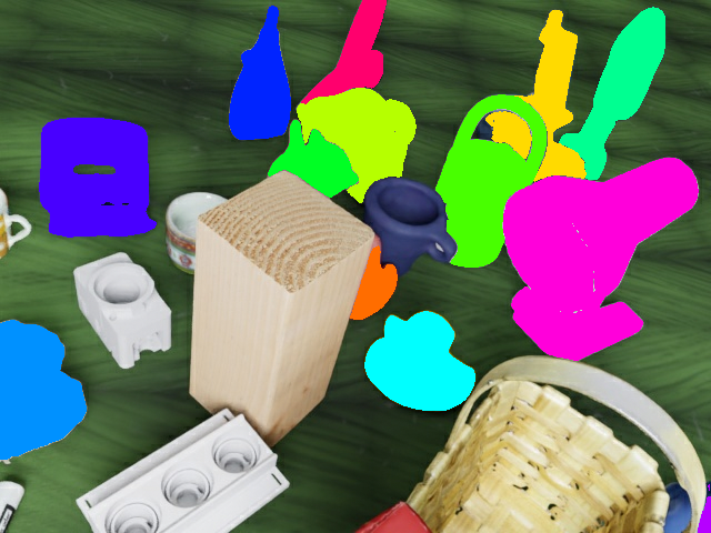
(a) input image and estimated mask

(b) estimated vector field (Base)

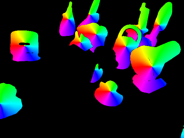
(c) estimated vector field (C/GCU)

(d) detail comparison 1

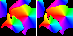
(e) detail comparison 2

Figure 7: Visual comparison of the estimated vector fields for a network with (C/GCU) and without (Base) the semantically guided operations. In the detail comparisons, Base is on the left, while C/GCU is on the right.

A.2 Characteristics of the Learned Confidence Maps

Fig. 8 shows the estimated vector fields and confidence maps for an image from LM-O using the 8-object model. The estimated 2D locations are highlighted by a white circle. The confidence values are normalised inside each semantic mask for clearer presentation. For the first keypoint (Fig. 8(b)), which is always in the centre of the object, the confidence is relatively constant in each mask, indicating that it is easy for the network to predict this point with high accuracy. In Fig. 8(c) and 8(d), it can be seen that the regions where the network predicts high confidence are often spatially close to the actual keypoint location. For example, for the tip of the tail of ’cat’ in Fig. 8(c), it is logical that the best prediction of the location can be made nearby. Moreover, for example, ’ape’ in Fig. 8(d) shows that the model predicts high reliability and thus computes the 2D position of a keypoint mainly from pixels near the object silhouette. Especially for non-textured objects, the silhouette provides important information about the orientation of the object. It seems appropriate that the vectors near the contour can be estimated with higher precision.

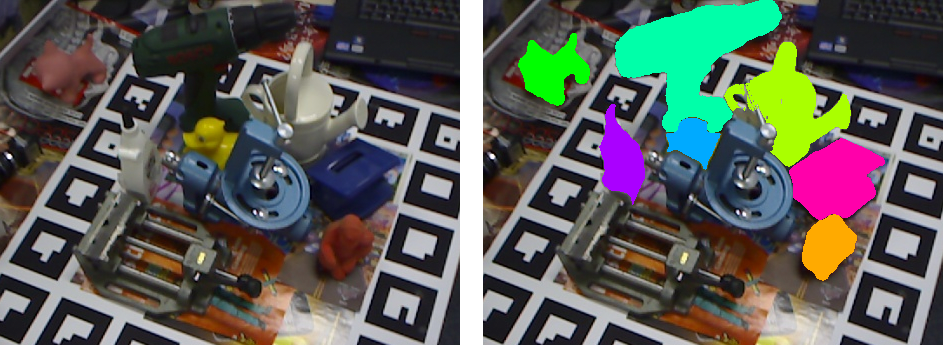
(a) Image and estimated mask

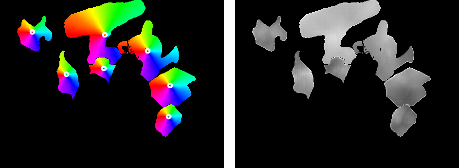
(b) Keypoint #1

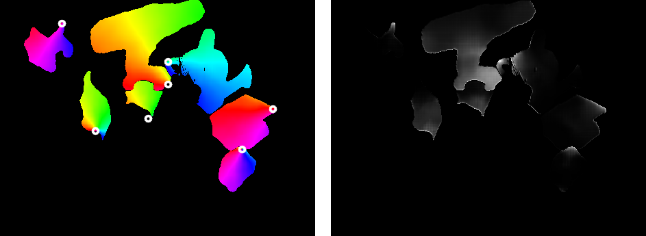
(c) Keypoint #4

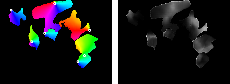
(d) Keypoint #5

Figure 8: Estimated vector fields and confidence maps for three out of nine keypoints.

Appendix B Additional Experiments

B.1 BOP Challenge Evaluation

In the BOP Challenge 2020 [Hodaň et al.(2020)Hodaň, Sundermeyer, Drost, Labbé, Brachmann, Michel, Rother, and Matas] multiple approaches submitted results for several pose estimation datasets, including LM-O with synthetic training. The results presented are in most cases significantly improved by subsequently inserted changes compared with the results from the original publications. We also evaluated our results against the BOP benchmark. It calculates an accuracy called Average Recall (AR), which is the average of the results for three pose error functions, Maximum Symmetry-Aware Projection Distance (MSPD), Maximum Symmetry-Aware Surface Distance (MSSD), and Visible Surface Discrepancy (VSD). Further details can be found in [Hodaň et al.(2020)Hodaň, Sundermeyer, Drost, Labbé, Brachmann, Michel, Rother, and Matas].

Table 6 lists the results of our procedure with this metric. CASAPose₈ is our final result for the 8-object case from the main paper. EPOS [Hodan et al.(2020)Hodan, Barath, and Matas, Hodaň et al.(2020)Hodaň, Sundermeyer, Drost, Labbé, Brachmann, Michel, Rother, and Matas], the only other single-stage multi-object method achieved an AR of 54.7, slightly higher than CASAPose. CASAPose_8* trained with minimally different hyper parameters (increasing $\lambda_{4}$ from $0.007$ to $0.01$), again achieves a slightly superior result, showing that both methods are similarly accurate. Still, our method is multiple times faster (468ms vs. 37 ms) . CDPNv2 [Li et al.(2019)Li, Wang, and Ji, Hodaň et al.(2020)Hodaň, Sundermeyer, Drost, Labbé, Brachmann, Michel, Rother, and Matas], the best method using only rgb images and no additional refinement (EPOS would be the second best method on LM-O with these properties), reaches an AR of $62.4$, but trains a single network for every object. They make numerous extensions to their original approach (adding more complicated domain randomisation and a more powerful backbone) that would potentially improve our method as well, but are out of scope of this paper. The innovations of our paper to convert a multi-stage (one network per object and bounding box detector) approach into a single-stage (one network for all objects without need for a bounding box detector) approach could be applied analogously to their method.

Arch.	DNN	$AR$	$AR_{MSPD}$	$AR_{MSSD}$	$AR_{VSD}$
EPOS [Hodan et al.(2020)Hodan, Barath, and Matas, Hodaň et al.(2020)Hodaň, Sundermeyer, Drost, Labbé, Brachmann, Michel, Rother, and Matas]	1/set	54.7	75.0	50.1	38.9
CASAPose8	1/set	54.2	74.3	49.4	39.0
CASAPose8*	1/set	55.4	75.3	50.8	40.2
CASAPose2x4	2/set	57.4	77.1	52.9	42.1

Table 6: Comparison of different variants of our method using the BOP benchmark on LM-O with EPOS [Hodan et al.(2020)Hodan, Barath, and Matas] in BOP configuration [BOP: Benchmark for 6D Object Pose Estimation(), Hodaň et al.(2020)Hodaň, Sundermeyer, Drost, Labbé, Brachmann, Michel, Rother, and Matas]. CASAPose_2x4 is the ’4 Obj. 2x’ result from Table 5 of the main paper using 2 notworks, each for 4 objects.

B.2 Ablation Study: Guided Decoder

We tested different versions of the semantically guided decoder for the 13-object configuration trained with DKR (Table 8). The first variant C/GU uses only guided upsampling and no guided convolution. Compared with CLADE (C) alone, this does not bring an improvement, since the increased accuracy during upsampling is cancelled out by the following regular convolution, which does not take the masks into account. Adding guided convolutions in the first 3 or 4 of 5 decoder blocks (C/GCU3, C/GCU4) improves the average 2DP and the average ADD/S. Between C/GCU3 and C/GCU4 no clear difference is visible. Comparing the final model C/GCU5 (with guided convolutions in all decoder blocks) with C/GCU4, the 2DP decreases by 0.6% on average, while an increase of 4.1% of ADD/S outweighs this. This makes this architecture the best among the tested ones.

B.3 Influence of Keypoint Regression

Table 8 compares different variants of the calculation of 2D keypoint positions. $LS_{1stComp.}$ is the variant used in our final model. It applies DKR on the largest connected component of each object class and clearly outperforms RANSAC voting ($PV_{RANSAC}$) [Peng et al.(2019)Peng, Liu, Huang, Zhou, and Bao] used with the same trained model. Interestingly, if a network learns to estimate confidence maps with DKR during training, also the results of the RANSAC voting improve ($PV_{RANSAC}$ compared with $PV_{RANSAC*}$). This suggests that least squares optimisation over all vectors in a region during training also improves the global accuracy of the estimated vectors. Applying DKR on a complete mask without connected component filtering ($LS_{All}$) deteriorates the performance, indicating that potential clutter in the estimated semantic masks should be removed before calculating the 2D positions. We tested DKR on the second largest connected component $LS_{2ndComp.}$ and see that it nearly never leads to a correct pose. So, at least for the case where only one object per class is visible, using only the largest connected components is very suitable. A proposal for adaptation to multi-instance scenarios is given in the main paper.

	LM-O		LM
	2DP	ADD/S	2DP	ADD/S
C	51.4	29.9	93.6	64.7
C/GU	50.7	30.0	93.9	62.9
C/GCU3	52.0	32.1	93.7	65.5
C/GCU4	52.7	31.9	93.5	64.9
C/GCU5	51.5	32.7	93.8	68.1

Table 7: Comparison of different versions of the semantically guided decoder using the 13-object model with DKR.

	2DP	ADD/S
$PV_{RANSAC*}$	49.2	26.7
$PV_{RANSAC}$	50.4	30.8
$LS_{All}$	45.3	29.7
$LS_{2ndComp.}$	7e-3	2e-3
$LS_{1stComp.}$	51.5	32.7

Table 8: Comparison of different variants of 2D keypoint calculation using the 13-object model (C/GCU5) on LM-O.

Appendix C Additional Details

C.1 Differentiable Keypoint Regression

The Differentiable Keypoint Regression uses a weighted Least Squares intersection of lines calculation, incorporating confidence scores as weights, as it is described e.g. in [Traa(2013)]. One system is constructed per keypoint per object. All systems are solved in parallel using tf.linalg.pinv to calculate the Moore-Penrose pseudo-inverse. DKR uses the softplus function to translate from the network output to the weights of the Least Squares calculations. It is a smooth approximation of the ReLU function that constraints the output of the network to be non negative. Compared with sigmoid, it allows to predict weights greater than 1. During training, we add a regularisation term to avoid drift of the Least Squares weights for DKR towards zero or infinity. The mean value in the foreground regions of each output map is $\ell 1$ regularised to be close to a constant value of 0.7.

C.2 Hyperparameter Choices

The losses $\mathcal{L}_{Seg}$, $\mathcal{L}_{Vec}$, $\mathcal{L}_{PV}$, and $\mathcal{L}_{Key}$ are weighted with the factors $\lambda_{1-4}$. Previous work weighted $\mathcal{L}_{Seg}$ and $\mathcal{L}_{Vec}$ equally ($\lambda_{1}=\lambda_{2}=1.0$) [Peng et al.(2019)Peng, Liu, Huang, Zhou, and Bao], or additionally added $\mathcal{L}_{PV}$ as a regularizer with much smaller weight [Yu et al.(2020)Yu, Zhuang, Koniusz, and Li]. In tests without DKR and $\mathcal{L}_{Key}$, we determined $0.015$ as a suitable choice for $\lambda_{3}$. This is larger than the recommendation of [Yu et al.(2020)Yu, Zhuang, Koniusz, and Li], but leads to stable convergence in our case. A reduction of the influence of $\mathcal{L}_{Vec}$ ($\lambda_{2}=0.5$) after including $\mathcal{L}_{Key}$ preserves the balance between segmentation ($\lambda_{1}$) and vector field prediction ($\lambda_{2-4}$). In summary, the weights were $\lambda_{1}=1.0$ , $\lambda_{2}=0.5$, $\lambda_{3}=0.015$ and $\lambda_{4}=0.007$.

As reported in Section B.1, we also trained a full model using $\lambda_{4}=0.01$ and observed a slight accuracy increase for LM-O (8 objects). However the 13-object model (LM) did not converge as good in this setting.

For models with two decoders (C and C/GCU), the calculation of $\mathcal{L}_{Vec}$ and $\mathcal{L}_{PV}$ evaluates only those locations where the estimated segmentation matches the true segmentation, which in our experience slightly improves the training result.

C.3 Further Details

• The Farthest Point Sampling (FPS) algorithm is used to calculate the 3D locations of the keypoints [Peng et al.(2019)Peng, Liu, Huang, Zhou, and Bao]. The keypoint set is initialised by adding the object centre. The 3D models of HB originate from a different 3D scan and have their origin in a different location than the models of LM. We aligned them with the Iterative Closest Point (ICP) algorithm and calculate a fixed compensation transformation for each model. It is applied to the 3D keypoints to make a comparison with HB’s ground truth.

• Pose estimation uses OpenCV’s cv::solvePnPRansac with EPnP [Lepetit et al.(2009)Lepetit, Moreno-Noguer, and Fua] followed by a call of cv::solvePnP with SOLVEPNP_ITERATIVE and the previous pose as ExtrinsicGuess.

• During training, we use scenes $0$-$48$ from the synthetic pbr LINEMOD images from [Hodaň et al.(2020)Hodaň, Sundermeyer, Drost, Labbé, Brachmann, Michel, Rother, and Matas] resulting in 49000 training images. Scene $49$ (1000 images) is kept for testing and is used in the ablation study.

• The experiments were conducted using Tensorflow 2.9 and use ADAM optimiser [Kingma and Ba(2015)]. Our custom layers use Tensorflow’s tf.function(jit_compile=True) for acceleration.

References

- [Aing et al.(2021)Aing, Lie, Chiang, and Lin] Lee Aing, Wen-Nung Lie, Jui-Chiu Chiang, and Guo-Shiang Lin. Instancepose: Fast 6dof pose estimation for multiple objects from a single RGB image. In Proc. ICCV Workshops, 2021.
- [Billings and Johnson-Roberson(2019)] Gideon Billings and Matthew Johnson-Roberson. Silhonet: An RGB method for 6d object pose estimation. IEEE Robotics and Automation Letters, 4(4):3727–3734, 2019.
- [Brachmann et al.(2014)Brachmann, Krull, Michel, Gumhold, Shotton, and Rother] Eric Brachmann, Alexander Krull, Frank Michel, Stefan Gumhold, Jamie Shotton, and Carsten Rother. Learning 6d object pose estimation using 3d object coordinates. In Proc. ECCV, 2014.
- [Cheng et al.(2020)Cheng, Collins, Zhu, Liu, Huang, Adam, and Chen] Bowen Cheng, Maxwell D Collins, Yukun Zhu, Ting Liu, Thomas S Huang, Hartwig Adam, and Liang-Chieh Chen. Panoptic-deeplab: A simple, strong, and fast baseline for bottom-up panoptic segmentation. In Proc. CVPR, 2020.
- [Dumoulin et al.(2017)Dumoulin, Shlens, and Kudlur] Vincent Dumoulin, Jonathon Shlens, and Manjunath Kudlur. A learned representation for artistic style. In Proc. ICLR, 2017.
- [Dundar et al.(2020)Dundar, Sapra, Liu, Tao, and Catanzaro] Aysegul Dundar, Karan Sapra, Guilin Liu, Andrew Tao, and Bryan Catanzaro. Panoptic-based image synthesis. In Proc. CVPR, 2020.
- [Gard et al.(2022)Gard, Hilsmann, and Eisert] Niklas Gard, Anna Hilsmann, and Peter Eisert. Combining local and global pose estimation for precise tracking of similar objects. In Proc. VISAPP, 2022.
- [Gatys et al.(2015)Gatys, Ecker, and Bethge] Leon A. Gatys, Alexander S. Ecker, and Matthias Bethge. A neural algorithm of artistic style. arXiv preprint arXiv:1508.06576, 2015.
- [He et al.(2016)He, Zhang, Ren, and Sun] Kaiming He, Xiangyu Zhang, Shaoqing Ren, and Jian Sun. Deep residual learning for image recognition. In Proc. CVPR, 2016.
- [Hinterstoisser et al.(2012)Hinterstoisser, Lepetit, Ilic, Holzer, Bradski, Konolige, and Navab] Stefan Hinterstoisser, Vincent Lepetit, Slobodan Ilic, Stefan Holzer, Gary Bradski, Kurt Konolige, and Nassir Navab. Model based training, detection and pose estimation of texture-less 3d objects in heavily cluttered scenes. In Proc. ACCV, 2012.
- [Hodan et al.(2020)Hodan, Barath, and Matas] Tomas Hodan, Daniel Barath, and Jiri Matas. Epos: Estimating 6d pose of objects with symmetries. In Proc. CVPR, 2020.
- [Hodaň et al.(2020)Hodaň, Sundermeyer, Drost, Labbé, Brachmann, Michel, Rother, and Matas] Tomáš Hodaň, Martin Sundermeyer, Bertram Drost, Yann Labbé, Eric Brachmann, Frank Michel, Carsten Rother, and Jiří Matas. Bop challenge 2020 on 6d object localization. In Proc. ECCV Workshops, 2020.
- [Hou et al.(2020)Hou, Ahmadyan, Zhang, Wei, and Grundmann] Tingbo Hou, Adel Ahmadyan, Liangkai Zhang, Jianing Wei, and Matthias Grundmann. Mobilepose: Real-time pose estimation for unseen objects with weak shape supervision. arXiv preprint arXiv:2003.03522, 2020.
- [Hu et al.(2019)Hu, Hugonot, Fua, and Salzmann] Yinlin Hu, Joachim Hugonot, Pascal Fua, and Mathieu Salzmann. Segmentation-driven 6d object pose estimation. In Proc. CVPR, 2019.
- [Ioffe and Szegedy(2015)] Sergey Ioffe and Christian Szegedy. Batch normalization: Accelerating deep network training by reducing internal covariate shift. In Proc. ICML, 2015.
- [Jung(2020)] Alexander B. Jung. imgaug. https://github.com/aleju/imgaug, 2020. [Online; accessed 29-July-2022].
- [Kaskman et al.(2019)Kaskman, Zakharov, Shugurov, and Ilic] Roman Kaskman, Sergey Zakharov, Ivan Shugurov, and Slobodan Ilic. Homebreweddb: Rgb-d dataset for 6d pose estimation of 3d objects. In Proc. ICCV Workshops, 2019.
- [Kingma and Ba(2015)] Diederik P. Kingma and Jimmy Ba. Adam: A method for stochastic optimization. In Proc. ICRL, 2015.
- [Lepetit et al.(2009)Lepetit, Moreno-Noguer, and Fua] Vincent Lepetit, Francesc Moreno-Noguer, and Pascal Fua. Epnp: An accurate o(n) solution to the pnp problem. International Journal of Computer Vision, 81(2):155–166, 2009.
- [Li et al.(2019)Li, Wang, and Ji] Zhigang Li, Gu Wang, and Xiangyang Ji. Cdpn: Coordinates-based disentangled pose network for real-time rgb-based 6-dof object pose estimation. In Proc. ICCV, 2019.
- [Li et al.(2021)Li, Hu, Salzmann, and Ji] Zhigang Li, Yinlin Hu, Mathieu Salzmann, and Xiangyang Ji. Sd-pose: Semantic decomposition for cross-domain 6d object pose estimation. In Proc. AAAI, 2021.
- [Liu et al.(2018a)Liu, Reda, Shih, Wang, Tao, and Catanzaro] Guilin Liu, Fitsum A. Reda, Kevin J. Shih, Ting-Chun Wang, Andrew Tao, and Bryan Catanzaro. Image inpainting for irregular holes using partial convolutions. In Proc. ECCV, 2018a.
- [Liu et al.(2018b)Liu, Shih, Wang, Reda, Sapra, Yu, Tao, and Catanzaro] Guilin Liu, Kevin J. Shih, Ting-Chun Wang, Fitsum A. Reda, Karan Sapra, Zhiding Yu, Andrew Tao, and Bryan Catanzaro. Partial convolution based padding. arXiv preprint arXiv:1811.11718, 2018b.
- [Liu et al.(2018c)Liu, Lehman, Molino, Such, Frank, Sergeev, and Yosinski] Rosanne Liu, Joel Lehman, Piero Molino, Felipe Petroski Such, Eric Frank, Alex Sergeev, and Jason Yosinski. An intriguing failing of convolutional neural networks and the coordconv solution. In Proc. NIPS, 2018c.
- [Manhardt et al.(2019)Manhardt, Arroyo, Rupprecht, Busam, Birdal, Navab, and Tombari] Fabian Manhardt, Diego Martin Arroyo, Christian Rupprecht, Benjamin Busam, Tolga Birdal, Nassir Navab, and Federico Tombari. Explaining the ambiguity of object detection and 6d pose from visual data. In Proc. ICCV, 2019.
- [Mazzini(2018)] Davide Mazzini. Guided upsampling network for real-time semantic segmentation. In Proc. BMVC, 2018.
- [Park et al.(2020)Park, Mousavian, Xiang, and Fox] Keunhong Park, Arsalan Mousavian, Yu Xiang, and Dieter Fox. Latentfusion: End-to-end differentiable reconstruction and rendering for unseen object pose estimation. In Proc. CVPR, 2020.
- [Park et al.(2019a)Park, Patten, and Vincze] Kiru Park, Timothy Patten, and Markus Vincze. Pix2pose: Pixel-wise coordinate regression of objects for 6d pose estimation. In Proc. ICCV, 2019a.
- [Park et al.(2019b)Park, Liu, Wang, and Zhu] Taesung Park, Ming-Yu Liu, Ting-Chun Wang, and Jun-Yan Zhu. Semantic image synthesis with spatially-adaptive normalization. In Proc. CVPR, 2019b.
- [Peng et al.(2019)Peng, Liu, Huang, Zhou, and Bao] Sida Peng, Yuan Liu, Qixing Huang, Xiaowei Zhou, and Hujun Bao. Pvnet: Pixel-wise voting network for 6dof pose estimation. In Proc. CVPR, 2019.
- [Rad and Lepetit(2017)] Mahdi Rad and Vincent Lepetit. Bb8: A scalable, accurate, robust to partial occlusion method for predicting the 3d poses of challenging objects without using depth. In Proc. ICCV, 2017.
- [Sock et al.(2020)Sock, Castro, Armagan, Garcia-Hernando, and Kim] Juil Sock, Pedro Castro, Anil Armagan, Guillermo Garcia-Hernando, and Tae-Kyun Kim. Tackling two challenges of 6d object pose estimation: Lack of real annotated rgb images and scalability to number of objects. arXiv preprint arXiv:2003.12344v1, 2020.
- [Sofiiuk et al.(2019)Sofiiuk, Barinova, and Konushin] Konstantin Sofiiuk, Olga Barinova, and Anton Konushin. Adaptis: Adaptive instance selection network. In Proc. ICCV, 2019.
- [Song et al.(2020)Song, Song, and Huang] Chen Song, Jiaru Song, and Qixing Huang. Hybridpose: 6d object pose estimation under hybrid representations. In Proc. CVPR, 2020.
- [Sundermeyer et al.(2018)Sundermeyer, Marton, Durner, Brucker, and Triebel] Martin Sundermeyer, Zoltan-Csaba Marton, Maximilian Durner, Manuel Brucker, and Rudolph Triebel. Implicit 3d orientation learning for 6d object detection from rgb images. In Proc. ECCV, 2018.
- [Tan et al.(2021)Tan, Chen, Chu, Chai, Liao, He, Yuan, Hua, and Yu] Zhentao Tan, Dongdong Chen, Qi Chu, Menglei Chai, Jing Liao, Mingming He, Lu Yuan, Gang Hua, and Nenghai Yu. Efficient semantic image synthesis via class-adaptive normalization. IEEE Transactions on Pattern Analysis and Machine Intelligence, 2021.
- [Thalhammer et al.(2021)Thalhammer, Leitner, Patten, and Vincze] Stefan Thalhammer, Markus Leitner, Timothy Patten, and Markus Vincze. Pyrapose: Feature pyramids for fast and accurate object pose estimation under domain shift. In Proc. ICRA, 2021.
- [Traa(2013)] Johannes Traa. Least-squares intersection of lines. University of Illinois Urbana-Champaign (UIUC), 2013.
- [Tremblay et al.(2018)Tremblay, To, Sundaralingam, Xiang, Fox, and Birchfield] Jonathan Tremblay, Thang To, Balakumar Sundaralingam, Yu Xiang, Dieter Fox, and Stan Birchfield. Deep object pose estimation for semantic robotic grasping of household objects. In Proc. CoRL, 2018.
- [Uhrig et al.(2017)Uhrig, Schneider, Schneider, Franke, Brox, and Geiger] Jonas Uhrig, Nick Schneider, Lukas Schneider, Uwe Franke, Thomas Brox, and Andreas Geiger. Sparsity invariant cnns. In Proc. 3DV, 2017.
- [Ulyanov et al.(2016)Ulyanov, Vedaldi, and Lempitsky] Dmitry Ulyanov, Andrea Vedaldi, and Victor S. Lempitsky. Instance normalization: The missing ingredient for fast stylization. arXiv preprint arXiv:1607.08022, 2016.
- [Wang et al.(2020a)Wang, Manhardt, Shao, Ji, Navab, and Tombari] Gu Wang, Fabian Manhardt, Jianzhun Shao, Xiangyang Ji, Nassir Navab, and Federico Tombari. Self6d: Self-supervised monocular 6d object pose estimation. In Proc. ECCV, 2020a.
- [Wang et al.(2019)Wang, Chen, Xu, Liu, Loy, and Lin] Jiaqi Wang, Kai Chen, Rui Xu, Ziwei Liu, Chen Change Loy, and Dahua Lin. Carafe: Content-aware reassembly of features. In Proc. ICCV, 2019.
- [Wang et al.(2020b)Wang, Kong, Shen, Jiang, and Li] Xinlong Wang, Tao Kong, Chunhua Shen, Yuning Jiang, and Lei Li. Solo: Segmenting objects by locations. In Proc. ECCV, 2020b.
- [Wen et al.(2020)Wen, Pan, Yang, and Wang] Yilin Wen, Hao Pan, Lei Yang, and Wenping Wang. Edge enhanced implicit orientation learning with geometric prior for 6d pose estimation. IEEE Robotics and Automation Letters, 5(3):4931–4938, 2020.
- [Xiang et al.(2018)Xiang, Schmidt, Narayanan, and Fox] Yu Xiang, Tanner Schmidt, Venkatraman Narayanan, and Dieter Fox. Posecnn: A convolutional neural network for 6d object pose estimation in cluttered scenes. In Robotics: Science and Systems (RSS), 2018.
- [Yang et al.(2021)Yang, Yu, and Yang] Zongxin Yang, Xin Yu, and Yi Yang. Dsc-posenet: Learning 6dof object pose estimation via dual-scale consistency. In Proc. CVPR, 2021.
- [Yu et al.(2019)Yu, Lin, Yang, Shen, Lu, and Huang] Jiahui Yu, Zhe Lin, Jimei Yang, Xiaohui Shen, Xin Lu, and Thomas S Huang. Free-form image inpainting with gated convolution. In Proc. ICCV, 2019.
- [Yu et al.(2020)Yu, Zhuang, Koniusz, and Li] Xin Yu, Zheyu Zhuang, Piotr Koniusz, and Hongdong Li. 6dof object pose estimation via differentiable proxy voting regularizer. In Proc. BMVC, 2020.
- [Zakharov et al.(2019)Zakharov, Shugurov, and Ilic] Sergey Zakharov, Ivan Shugurov, and Slobodan Ilic. DPOD: 6d pose object detector and refiner. In Proc. ICCV, 2019.
- [Zhang et al.(2021)Zhang, Zhao, Guan, Peng, and Peng] Shaobo Zhang, Wanqing Zhao, Ziyu Guan, Xianlin Peng, and Jinye Peng. Keypoint-graph-driven learning framework for object pose estimation. In Proc. CVPR, 2021.
- [BOP: Benchmark for 6D Object Pose Estimation()] BOP: Benchmark for 6D Object Pose Estimation. Submission: EPOS-BOP20-PBR/LM-O. https://bop.felk.cvut.cz/sub_info/1382/, 2020. [Online; accessed 27-July-2022].