KIC 7955301: a hierarchical triple system with eclipse timing variations and an oscillating red giant

KIC 7955301 is a hierarchical triple system with clear eclipse timing and depth variations that was discovered by the Kepler satellite during its original mission. It is composed of a non-eclipsing primary star at the bottom of the red giant branch on a 209-day orbit with a K/G-type main-sequence inner eclipsing binary, orbiting in 15.3 days. This system was noted for the large amplitude of its eclipse timing variations (over 4 hours), and the detection of clear solar-like oscillations of the red-giant component, including p-modes of degree up to $l=3$ and mixed $l=1$ modes. The system is a single-lined spectroscopic triple, meaning that only spectral lines from the red giant are trackable along the orbit. We perform a dynamical model by combining the 4-year-long Kepler photometric data, eclipse timing variations and radial-velocity data obtained with the high resolution spectrometers ARCES of the 3.5-m ARC telescope at Apache Point observatory and SOPHIE of the 1.93-m telescope at Haute Provence Observatory. The “dynamical” mass of the red-giant component is determined with a 2 % precision at $1.30^{+0.03}_{-0.02}M_{\odot}$. We perform asteroseismic modeling based on the global seismic parameters and on the individual frequencies. Both methods provide an estimate of the mass of the red giant that matches the dynamical mass within the uncertainties. Asteroseismology also reveals the rotation rate of the core ($\approx 15$ days), the envelope ($\sim 150$ days), and the inclination ($\sim 75^{\circ}$) of the red giant. Three different approaches lead to estimating the age to range between 3.3 and 5.8 Gyr, which highlights the difficulty of determining stellar ages despite the exceptional wealth of information available for this system. On short timescales, the inner binary exhibits eclipses with varying depths during a $7.3$-year long interval, and no eclipses during the consecutive $11.9$ years. This is why Kepler could detect its eclipses, TESS will not, and the future ESA PLATO mission should. Over the long term, the system appears to be stable and owes its evolution to the evolution of its individual components. This triple system could end its current smooth evolution by merging by the end of the red giant branch of the primary star because the periastron distance is $\approx 142R_{\odot}$, which is close to the expected radius of the red giant at the tip of the RG branch.

1 Introduction

Among the 5000 stars that are visible with the naked eye, about 2000 are known to be multiple-star systems. Naked-eye stars are a small fraction of the Milky Way, but are reasonably representative of the incidence of binarity, which is estimated to be between 50 and almost 100 % (e.g., Eggleton 2006). Some systems are close enough to be in contact, others are far apart enough to evolve almost independently. Binary systems are known with orbital periods as short as 0.2 days or as long as thousands of years. Studying multiple-star systems is thus important for understanding the evolution of our Galaxy.

Stars in multiple systems are also precious benchmarks for calibrating asteroseismology when it is possible to measure the mass of the oscillating star independently from its oscillation properties. This is the case with double-lined spectroscopic binary (SB2) where the components eclipse each other, or optically resolved binary systems. Hitherto, all solar-like oscillators belonging to eclipsing binary stars (EBs) are red giants (RGs) detected by the Kepler mission (Hekker et al. 2010; Gaulme et al. 2013, 2014; Beck et al. 2014, 2015; Kuszlewicz et al. 2019; Benbakoura et al. 2021). So far, fourteen wide SB2/EBs including an oscillating RG have been fully characterized with the help of ground-based radial-velocity support (Frandsen et al. 2013; Rawls et al. 2016; Gaulme et al. 2016; Brogaard et al. 2018; Themeßl et al. 2018; Benbakoura et al. 2021). Three more bona fide oscillating RGs in EBs were reported by Gaulme & Guzik (2019), and are currently under study. Beyond EBs, it is also possible to determine the masses of stars belonging to visual multiple-systems, where individual components are spatially resolved, which allows retrieval of their projected orbits, provided radial velocities are available too. So far, very few of such systems include solar-like pulsators (Marcadon et al. 2018; Metcalfe et al. 2020). The drawback of such systems is that the orbits are long and getting accurate orbital parameters can take decades and rely on heterogeneous datasets. Finally, hierarchical triple systems are promising types of benchmarks; they are composed of a close binary with a relatively distant companion (e.g., Tokovinin 1997; Ford et al. 2000; Borkovits et al. 2003). Depending on their orbital configurations, the presence of eclipses and significant eclipse timing variations (ETVs), it can be possible to determine the masses of their components (Derekas et al. 2011; Carter et al. 2011; Borkovits et al. 2016).

KIC 7955301 is a hierachical triple system composed of a young RG and a pair of small main-sequence stars that was observed for nearly four consecutive years by the original NASA Kepler mission (Borucki et al. 2011) at long (29.4244-minute cadence). It was pointed out by Gaulme et al. (2013) and Rappaport et al. (2013) who noticed its outstanding eclipse timing, depth and duration variations. The pair of main-sequence stars shows partial eclipses, but the RG does not eclipse the inner binary. The eclipse timings show a periodicity of about 208.6 days, while the pair of MS stars orbit in 15.3 days. The precession of the orbital plane of the MS stars is quite visible as well, and has a period longer than the time series. This system was part of the cohort of systems with ETVs studied by Borkovits et al. (2016). From eclipse timing only, they estimated the mass of the RG to be $1.5\pm 0.5M_{\odot}$ and the total mass of the MS pair to be $2.2\pm 0.8M_{\odot}$. From asteroseismic scaling relations and a quick look at the mixed dipole ($l=1$) modes, Gaulme et al. (2013) inferred the RG mass to be $1.2\pm 0.2M_{\odot}$, the radius $5.9\pm 0.2R_{\odot}$, and the core rotation of about 30 days. By considering that asteroseismic scaling relations tend to slightly overestimate stellar masses for RGs (Gaulme et al. 2016), the RG is likely a descendent of an F-type star that had a convective envelope during the MS and that is expected to rotate slowly.

With this paper, we firstly aim at testing our ability to measure accurate masses in hierarchical triple systems. We know it is possible to determine the mass of a star that belongs to an eclipsing binary down to 1 % (e.g., Maxted et al. 2020). However, no study has specifically been developed for measuring the mass of an oscillating star in a hierarchical triple that is a single-lined spectroscopic triple system (ST1). We note that the famous RG in the hierarchical triple system HD 181068 (Derekas et al. 2011), observed by Kepler, is triply eclipsing and does not show any oscillations, likely because of the mode suppression observed in short period multiple systems (Gaulme et al. 2020). Given the clear ETVs and the clear oscillations of the RG, KIC 7955301 appears to be an ideal case for testing our methods on hierarchical triple systems with an oscillating component. Subsequently, the approaches described here should be extended to all known triple with ETVs that include an oscillating component (Gaulme et al. 2013).

The second objective is a rather unique opportunity to study an RG star in greater detail, thanks to the multiple approaches used simultaneously to give a clear picture of the system. Our study makes use of the Kepler photometric data and high-resolution optical spectra obtained with the 3.5-m telescope at Apache Point observatory, and with the échelle spectrograph SOPHIE of the 1.93-m telescope at the Haute-Provence Observatory (Sect. 2). The spectra are used to both determine the radial velocities and the atmospheric parameters (Sect. 3). The Kepler light curves are used to both analyze the eclipses for the asteroseismic analysis (Sect. 4) and the dynamical modeling (Sect. 5). Finally, the deduced parameters – oscillation frequencies, orbital parameters, etc. – are used to optimize a stellar evolution model (Sect. 6).

Table 1: Archival properties of the KIC 7955301 triple System.

Parameter	Value
RA (J2000)	$19:20:45$
Dec (J2000)	$+43:43:26$
$K_{\mathrm{p}}$a	$12.672$
$G$b	$12.6283\pm 0.0002$
$G_{\rm BP}^{b}$	$13.2017\pm 0.0012$
$G_{\rm RP}$b	$11.9340\pm 0.0009$
Bc	$14.082\pm 0.043$
Vd	$12.901\pm 0.008$
g′d	$13.419\pm 0.045$
r′d	$12.553\pm 0.043$
i′d	$12.323\pm 0.026$
Je	$10.992\pm 0.023$
He	$10.487\pm 0.018$
Ke	$10.385\pm 0.011$
W1f	$10.323\pm 0.023$
W2f	$10.409\pm 0.020$
W3f	$10.310\pm 0.056$
W4f	$9.118$
$T_{\rm eff}$ (K)c	$4805\pm 75$
Distance (pc)g	$1375\pm 35$
${\rm[M/H]}^{c}$	$0.1163\pm 0.0072$
$E(B-V)^{c}$	$0.044$
$\mu_{\alpha}$ (mas  ${\rm yr}^{-1}$)h	$-0.86\pm 0.02$
$\mu_{\delta}$ (mas  ${\rm yr}^{-1}$)h	$-8.59\pm 0.02$

2 Observations

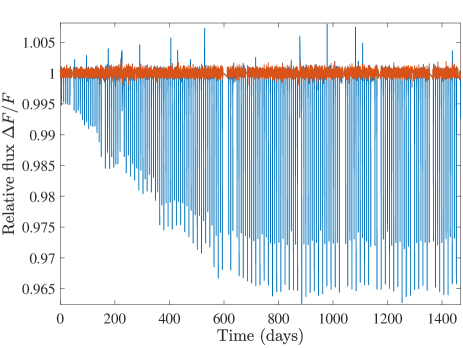
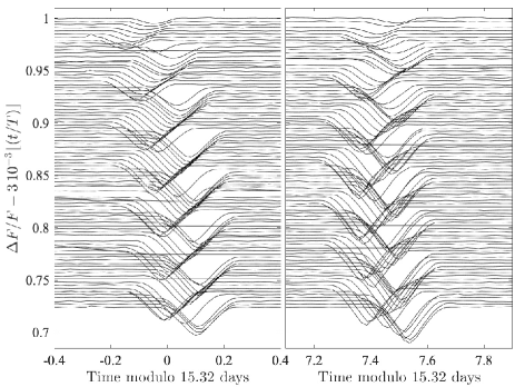
Figure 1: Kepler light curve of KIC 7955301. Top panel: relative flux as a function of time, where $t=0$ is the first day of data. The blue curve is the stitched light curve, whereas the orange curve has the eclipses removed and is used for asteroseismic analysis. Bottom panel: stitched lightcurve folded over the inner binary orbital period (15.32 days), where consecutive eclipses are vertically offset by 0.003 to ease the visibility of the transit depth and timing variations.

2.1 The Kepler light curve

We worked with the Kepler public light curves that are available on the Mikulski Archive for Space Telescopes (MAST). Two types of time series are available: the Simple Aperture Photometry (SAP) and the Pre-search Data Conditioning Simple Aperture Photometry (PDC-SAP) light curves. The latter consists of time series that were corrected for discontinuities, systematic errors and excess flux due to aperture crowding (Twicken et al. 2010). They do not meet our requirements for monitoring possible rotational modulation or eclipse depth, which are often altered during the process (e.g., García et al. 2014; Gaulme et al. 2014). We thus made use of the SAP data to preserve any possible long-term signal. This choice entails our own detrending and stitching operation on the light curves while ensuring that the rotational modulation is preserved after each interruption of the time series. The methods employed to clean the time series are detailed in Gaulme et al. (2016).

For asteroseismology, light curves with eclipses are an issue because their signal contaminates the Fourier domain, in which we perform the asteroseismic analysis. We tried two different approaches to remove the eclipses from the time series before computing its power density spectrum. The first approach is better in principle: it consists of modeling each eclipse with a typical eclipse function, for example that from Mandel & Agol (2002) for fitting exoplanetary transits, and then subtracting the model from the light curve. However, this approach, as noted in Gaulme et al. (2016), is less efficient than simply clipping out the eclipses, followed by gap filling with a second-order polynomial. Indeed, an eclipse model is always a little imperfect and when subtracted about 100 times (the number of eclipses during the Kepler run) they still damage the Fourier transform, unlike eclipse removal and filling. Figure 1 (top panel) shows the original time series along with the time series with no eclipses that is used for analyzing the RG oscillations. The bottom panel highlights the eclipses variations in the form of a folded light curve where a shift was introduced between consecutive orbits. Eclipse depth varies from 0.5 to almost 4 %, timing by about 4 hours, and duration from approximately 4.3 to 6.7 hours.

2.2 High-resolution optical spectra

From 2012 to 2019, we were granted time on the ARCES échelle spectrograph of the 3.5-m telescope of the Astrophysical Research Consortium (ARC) at Apache Point observatory (APO), which covers the whole visible domain at an average resolution of $31,000$ (Wang et al. 2003). This allowed us to monitor KIC 7955301 23 times, among observations of other RGs in multiple systems. Even though the ARC échelle spectrograph was not designed for precise RV measurements, it has successfully been used for this purpose in earlier work (e.g., Rawls et al. 2016; Gaulme et al. 2016; Benbakoura et al. 2021). The measurement error reported in these papers is about 0.5 km s^-1 for an RG spectrum with a signal-to-noise ratio (S/N) between 10 and 20. In practise our spectra have a S/N ranging from 10 to 25. The ARCES optical spectra were processed and analyzed in the same way as in Gaulme et al. (2016) and Benbakoura et al. (2021) and we refer to these papers for details.

In addition to the APO spectrograph, we were granted observing time on the SOPHIE échelle spectrograph at the 1.93-m telescope at the Haute-Provence Observatory (OHP). We obtained spectra of KIC 7955301 on June 8, 9 and October 9, 2018. The SOPHIE data processing pipeline directly provides the radial velocities from the spectra. We refer the reader to Santerne et al. (2011b, a) for details on the data reduction and radial-velocity measurement based on SOPHIE spectra.

3 Spectroscopic analysis

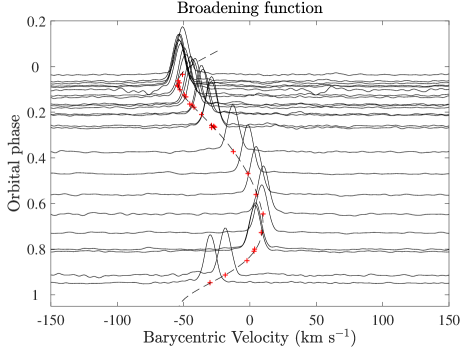
Figure 2: Broadening function of the 23 spectra taken with the échelle spectrometer of the 3.5-m ARC telescope at Apache Point observatory. Spectra were sorted by increasing orbital phase. The position along the $y$ axis corresponds with the orbital phase. Barycentric velocity corrections are included in the BF computation. The radial velocity data are indicated with the red plus symbols and their best-fit Keplerian-orbit model by a dashed line.

3.1 Radial-velocities

From the reduced one-dimensional spectra obtained at APO, we computed the radial velocities with the Broadening-Function technique (BF, Rucinski 2002). The fundamental hypothesis of this method is that the observed spectrum is the theoretical spectrum convolved with a broadening function that accounts for stellar rotation and instrumental effects. The BF technique deconvolves the observed spectrum by the theoretical one to extract the BF. For SB2 systems, the BF shows two peaks, one per component.

We employed the theoretical spectra generated by the PHOENIX BT-Settl code (Allard et al. 2003), which were computed with the solar abundances derived by Asplund et al. (2009). As in Gaulme et al. (2016) and Benbakoura et al. (2021), we used templates of MS stars ($T_{\rm eff}=6200$ K) to maximize the chance of detecting the signal from the companion star. Such a choice actually also helps the deconvolution of the RG spectrum because the large number of absorption lines in RG spectra tends to increase the noise in the BF profiles when the original spectra do not have an excellent S/N, which is our case. We computed the BF by making use of the wavelength range 4500 and 5800 Å. Our final RV data were obtained after correcting the BF profiles from the barycentric corrections, which account for the rotation and revolution of the Earth with respect to the target. We computed the barycentric corrections with the PyAstronomy routine helcorr, which is based on the Piskunov & Valenti (2002) algorithm.

All the radial velocities we produced in this work are compiled in Table 5 and displayed in Fig. 2 together with the series of BF profiles. For illustration purposes we overplot data points with a fit performed with a simple Keplerian orbit. This allows us to estimate the standard deviation of the measurements to be about 0.70 km s^-1. We note that employing a Keplerian orbit is a very simplistic approach as KIC 7955301 is a triple system. In Sect. 5 we show that the argument of periastron of the outer orbit changed by about 20^∘ during the four years of Kepler observations, meaning that a simple Keplerian orbit is not sufficient to accurately model the RG orbit.

3.2 Disentangling the spectra

A proper estimate of the atmospheric parameters of the RG and possibly of the inner binary components requires disentangling the spectra. For a triple system with such a large flux contrast between the evolved primary component and the inner dwarf binary, it is not an easy task. The spectral lines of the three components are diluted and it is challenging to disentangle the individual contributions to the continuum without knowing the light ratio. It is straightforward to get the ratio from a light curve when all components eclipse each other. Unfortunately, in our case, the RG is not eclipsing with the inner pair. The remaining method for measuring the light ratio and distentangling the spectra consists of scaling the absorption lines from synthetic spectra to the series of observed spectra (Pavlovski et al. 2009, 2018, and references therein).

According to the dynamical model presented in the following sections, the contribution of the main-sequence components to the total luminosity is close to 10 %, which implies that we cannot visualize their signatures neither in the BF profile, nor in the spectra. Nevertheless, very faint components have been revealed by spectral disentangling even at a level of only 1-2 % of the total light, such as the M dwarf in the EB V530 Ori (Torres et al. 2014), the Roche-lobe filling giant in the inner EB of the Algol triple system (Kolbas et al. 2015), the main sequence companions of the RGs in EBs (e.g., Gaulme et al. 2016; Hełminiak et al. 2017; Brogaard et al. 2018; Themeßl et al. 2018; Benbakoura et al. 2021).

In spectral disentangling as originally formulated by Simon & Sturm (1994), the spectra of the individual components are simultaneously reconstructed with an optimization of the orbital elements of the multiple-star system. The problem consists of solving the matrix equation $A\cdot x=b$, where the vector $x$ represents the unknown individual spectra of the components – which we aim at extracting – and $b$ all of the observed spectra. The design matrix $A$ is constructed from Doppler shifts for a given set of the orbital elements and exposure dates. $A$ could also contain light dilution factors, if known. Since the set of linear equations are overdetermined, the solution may be calculated with the linear-algebra technique known as singular value decomposition. In our particular case, the RVs for the RG component are measured by the BF (Sect. 3.1, and Table 5). From the dynamical model of the system described in Sect. 5, we computed the expected values of the RVs of the components of the inner binary.

The spectral disentangling is performed with the code cres (Ilijic 2004), which is based on the Simon & Sturm (1994) method for spectral disentangling in the visible domain. In cres, the RVs, light dilution factors of each component, and the observed spectra are inputs. The observed spectra should be given in units of wavelength. The observed spectra do not need to be in an uniform scale, and the spectra from different spectrographs do not need to be resampled first. Any portion of the observed spectra could be masked out to exclude undesired wavelength regions.

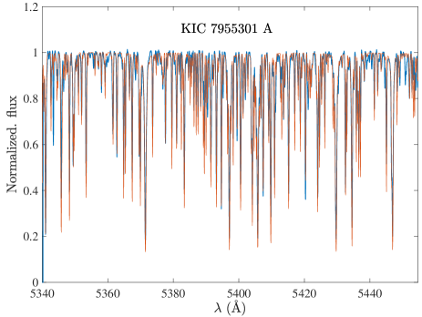
Figure 3: A sample region of the mean spectra of the individual components of the system obtained by disentangling the APO spectra. Top panel: spectrum of the RG component (blue line) and its best fit obtained with the gssp code (red) from 5340 to 5450Å. Bottom panel: spectra of the inner binary system Ba and Bb (blue lines) together with their best-fit synthetic spectra (red lines). The optimal values representing the best fits are listed in Table 2.

Altogether, we use the 23 high-resolution échelle spectra obtained at APO (Sect. 2.2). Spectra have a S/N from $\sim 5$ to 60, with an average S/N $\simeq 27$, as measured in several short line-free windows near 5500 - 5600 Å. The S/N was then used to assign weights to the observed spectra. We note that the code actually allows an assignment of the weights to individual pixels, another feature advantageous in the wavelength-domain disentangling, but we did not use this option, assuming it is sufficient to take the weight per spectrum, and not per pixel. The selected spectral segments had various lengths, from about 40 to 90 Å, always taking into account overlapping regions which serve to double-check the quality of our disentangling.

It is known that without any substantial change in the fractional light of the components in the course of an orbital cycle, there is no unique solution in reconstruction of the individual spectra of the components (Pavlovski & Hensberge 2005). One possibility is to optimize the light dilution factors in the calculations of the components’ spectra, but with dominant fractional light contribution of the RG component, which is not eclipsing with the inner pair of the MS stars, this would be meaningless. The best option is to perform spectral disentangling in a pure separation mode, and then determine fractional light contribution for each component from its spectral characteristics.

The reconstruction of the individual spectra of all three components was performed in the wavelength range $[5100,5650]$ Å. In addition, the spectral range of the disentangled spectrum for the RG component was extended to the range $[4700,6825]$ Å. In the latter case, our intention was to cover the Balmer lines H$\alpha$, and H$\beta$, as well as the sodium doublet Na i at $\lambda\lambda$ 5890, and 5896 Å. Some portions of the reconstructed spectra are shown in Fig. 3. It is evident from a bottom panel of Fig. 3 showing reconstructed spectra for the stars in the inner (eclipsing) pair that the signatures of the stellar spectra are successfully revealed, albeit the noise level is large. We can estimate the gain in the S/N for the spectra of the disentangled components by simple calculations, since spectral disentangling, in principle, is working as co-addition of the observed spectra. By assuming random noise with an average S/N $\simeq 27$, the 23 spectra should lead to total S/N of about 130. Of this, the RG spectrum benefits most since it contributes about 91 % of the total light, as is determined later in this section. The other two components share the remaining $\sim 9$ % – given their contribution is similar (Sect. 5, Table 4) –, meaning that the S/N of their reconstructed spectra is about 5-6. Thus, their spectral signatures are revealed only thanks to the gain of S/N caused by the spectral disentangling. The successful isolation of the spectra for the stars in the inner system, which is based on the RVs calculated from the predicted orbit, is an encouraging confirmation of the correctness of the dynamical model.

The deepest absorption lines in the disentangled spectrum of the RG component are due to Mg i$b$ triplet lines at 5167, 5172, and 5183 Å, and Na i D doublet at 5890, and 5896 Å. The depths of these sets of spectral lines constrain the fractional light contribution of the RG to the total light of the system. A limit defined by the physical solution is at 89%, which is corroborated with the optimal fitting (Table 2).

It is well established by observational evidence that lithium is depleted in the majority of giants (Brown et al. 1989). There are rare exceptions known as Li-rich giants with abundances $A({\rm Li})>1.5$ (a scale where the number of hydrogen atoms $\log N({\rm H})=12.0$). Examination of the disentangled spectrum of the RG component of KIC 7955301 shows almost no trace of the Li i resonance doublet at 6708 Å. An estimate of an upper limit of the lithium abundance was made with a comparison to the synthetic line profiles. The calculations were performed assuming local thermodynamic equilibrium with model atmospheres calculated with Atlas9 (Castelli & Kurucz 2003), while line profiles for Li i 6708 Å are calculated with spectrum synthesis code uclsyn (Smith 1992). The atomic data are from Yan et al. (1998). We were able to establish only an upper limit in lithium abundance $A({\rm Li})<-1.0$ dex. This is a common lithium abundance found in modern massive spectroscopic surveys (Luck & Heiter 2007; Buder et al. 2018; Charbonnel et al. 2020).

3.3 Stellar atmospheric parameters

Table 2: Best-fit parameters deduced from the analysis of the atmospheric parameters.

Red giant (star A)
Run A	$T_{\mathrm{eff}}$	[K]	$4720\pm 105$
	$\log g$	[dex]	3.0 (fixed)
	$v_{\mathrm{micro}}$	[km s-1]	$1.44\pm 0.35$
	$v\sin i$	[km s-1]	$6.4\pm 1.2$
	dilution factor		$0.91\pm 0.08$
	$[\mathrm{M}/\mathrm{H}]$	[dex]	$-0.01\pm 0.12$
Run B	$T_{\mathrm{eff}}$	[K]	$4760\pm 110$
	$\log g$	[dex]	3.1 (fixed)
	$v_{\mathrm{micro}}$	[km s-1]	$1.36\pm 0.35$
	$v\sin i$	[km s-1]	$6.3\pm 1.2$
	dilution factor		$0.92\pm 0.07$
	$[\mathrm{M}/\mathrm{H}]$	[dex]	$0.03\pm 0.12$
Run C	$T_{\mathrm{eff}}$	[K]	$4700\pm 155$
	$\log g$	[dex]	$2.95\pm 0.40$
	$v_{\mathrm{micro}}$	[km s-1]	$1.31\pm 0.35$
	$v\sin i$	[km s-1]	$6.6\pm 1.3$
	dilution factor		$0.91\pm 0.08$
	$[\mathrm{M}/\mathrm{H}]$	[dex]	$-0.01\pm 0.17$
Inner binary (stars Ba and Bb)
Ba	$T_{\mathrm{eff}}$	[K]	$5620\pm 580$
	$\log g$	[dex]	4.5 (fixed)
	$v_{\mathrm{micro}}$	[km s-1]	2.0 (fixed)
	$v\sin i$	[km s-1]	$19.0\pm 5.5$
	dilution factor		$0.043\pm 0.013$
	$[\mathrm{M}/\mathrm{H}]$	[dex]	0.0 (fixed)
Bb	$T_{\mathrm{eff}}$	[K]	$5330\pm 550$
	$\log g$	[dex]	4.5 (fixed)
	$v_{\mathrm{micro}}$	[km s-1]	2.0 (fixed)
	$v\sin i$	[km s-1]	$8.9\pm 7.5$
	dilution factor		$0.025\pm 0.009$
	$[\mathrm{M}/\mathrm{H}]$	[dex]	0.0 (fixed)

For the analysis of the disentangled spectra of all three components of the KIC 7955301 system, we employed the Grid Search in Stellar Parameters (gssp Tkachenko 2015) software package, specifically its gssp_single module. It is a grid search-based spectrum analysis algorithm that (on the fly) generates synthetic spectra in an arbitrary wavelength range based on a pre-computed grid of model atmospheres, and performs a comparison between the observed spectrum and each synthetic spectrum from the grid in the $\chi^{2}$ statistical framework. The reported 1-$\sigma$ uncertainties are computed from the $\chi^{2}$-statistics and taking into account possible correlations between the free parameters. The gssp algorithm allows for the simultaneous optimization of the effective temperature, surface gravity, micro- and macro-turbulent velocities, projected rotational velocity, and metallicity of the star. Optionally, one can also optimize for the degree of the light dilution in the spectrum due to the star being a member of a binary and/or higher order multiple system.

In this study, we employ the grid of LLmodels model atmospheres (Shulyak et al. 2004) and opt for inclusion of the light dilution factor into the optimization to account for a priori unknown dilution of the disentangled spectrum of each of the three stellar components under the analysis. The light dilution factor is assumed to be wavelength independent, which is a fair assumption for the RG component given its by far most dominant ($>$ 90%) contribution to the composite spectrum of the system, as well as for the two main-sequence components given the limited wavelength interval of some 500 Å that could be used for the disentangling. We additionally note that the macro-turbulent velocity parameter was ignored in the analysis of all three stellar components of the system, and we additionally fixed $\log\,g$ for both main-sequence components to the values inferred from the light curve solution, micro-turbulent velocity to 2 km s^-1, and assumed solar chemical composition ([M/H] = 0.0 dex) for both of them. The choice to fix so many parameters in the spectrum analysis of the main-sequence components is dictated by their small cumulative contribution ($<$ 8-10%) to the total light of the system, and hence their very noisy disentangled spectra. The consequence of fixing the macro-turbulent velocity parameter for the RG component is that the $v\,\sin i$ value reported is in fact representative of the combined spectral line broadening due to the effects of rotation and macroturbulence. Finally we note that we explored three different options in the analysis of the RG spectrum, namely fixing the surface gravity to the two values inferred from the light curve solution and reported in Table 2, and treating $\log\,g$ as a free parameter.

4 Asteroseismic analysis

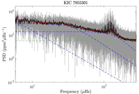
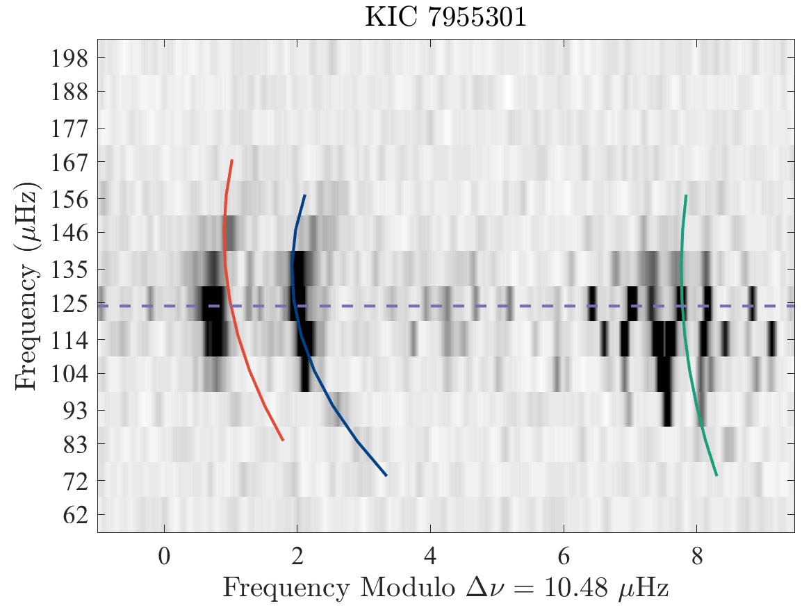
Figure 4: Oscillation spectrum of KIC 7955301. Top panel: power spectral density of the time series after eclipse removal and filling. The red dashed line represents the stellar background noise: it is the sum of the blue dashed lines (correlated noise Harvey profiles) and the green dashed line (white noise). The plain red line represents the fit of the power spectrum including the stellar background and the Gaussian envelope of the oscillations. Bottom panel: échelle diagram associated with the frequency spacing $\Delta\nu=10.48\,\mu$Hz. Colored lines indicate the oscillation universal pattern, where blue is $l=0$, green $l=1$, and red $l=2$. Modes of degree $l=3$ are visible half way in between the $l=0$ and $l=1$ ridges. The horizontal dashed line indicates the location of $\nu_{\mathrm{max}}$.

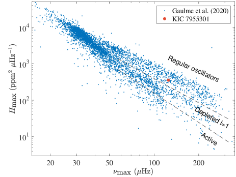
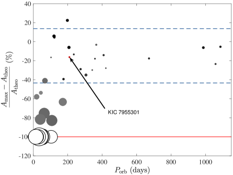
Figure 5: Oscillation amplitude. Top panel: height of the Gaussian envelope used to model the contribution of the oscillations to the stellar background. The red dot highlights the position of KIC 7955301 with respect to a sample of 4500 RGs analyzed by Gaulme et al. (2020) indicated in blue. The sample splits into three categories: the oscillators with regular amplitude, those with depleted $l=1$ modes, and the active RGs that show a global mode suppression ($l=0,1,2,3$). KIC 7955301 falls in the regular oscillators. Bottom panel: amplitude of the largest $l=0$ mode of KIC 7955301 compared with those of the 35 RGs in EBs that were studied by Benbakoura et al. (2021). The figure displays the relative difference between expected and measured oscillation amplitudes (%) as a function of orbital period $P_{\mathrm{orb}}$ (days). The red line indicates 0, i.e., stars whose oscillations are not detected. The two dashed blue lines represent the region in which relative mode amplitude lies for systems with orbital periods longer than 180 days within two sigma. The size of each symbol represents the amplitude of stellar variability (large means variable; small not variable), and the gray scale indicates the pulsation mode amplitude (white-no modes; black-large amplitude).

4.1 Global oscillation properties

The stellar granulation and accurate values of $\nu_{\mathrm{max}}$ and mode amplitude $H_{\mathrm{max}}$ are estimated by fitting the power spectrum (Fig. 4) as commonly performed in asteroseismology (Kallinger et al. 2014), and already used in Gaulme et al. (2016). Following Kallinger et al. (2014), the power density spectrum is fitted by

$$S(\nu)=N(\nu)+\eta(\nu)\left[B(\nu)+G(\nu)\right],$$ (1)

where the $N$ is the function describing the noise, $\eta$ is a damping factor originating from the data sampling, $B$ is the sum of three “Harvey” functions (super Lorentzian functions centered on 0), and G is the Gaussian function that accounts for the oscillation excess power

$$G(\nu)=H_{\mathrm{max}}\exp{\left[-\frac{(\nu-\nu_{\mathrm{max}})^{2}}{2\sigma^{2}}\right]}.$$ (2)

The terms $\nu_{\mathrm{max}}$ and $H_{\mathrm{max}}$ are the central frequency and height of the Gaussian function. The best-fit values are: $\nu_{\mathrm{max}}=124.89\pm 0.33\ \mu$Hz, $H=354.2\pm 10.5$ ppm $\mu$Hz^-1, and $\sigma=12.5\pm 0.4\,\mu$Hz.

A first estimate of $\Delta\nu$ is performed with the envelope of the autocorrelation function (EACF) developed by Mosser & Appourchaux (2009) from the whitened power spectral density (power spectrum divided by background function). From the EACF, $\Delta\nu=10.46\pm 0.05$. Then, we used the universal pattern of RGs introduced by Mosser et al. (2011) to correct it. The principle of this method is to compare the measured oscillation frequencies to a theoretical law, the so-called universal pattern, predicting the variations of these frequencies as a function of $\Delta\nu$ and the radial order. That way, the value of $\Delta\nu$ is revised to $10.49\pm 0.02\ \mu$Hz.

We then compute a proxy of the stellar masses and radii using the asteroseismic scaling relations that were originally proposed by Kjeldsen & Bedding (1995) for SL MS oscillators, and then successfully applied to RGs (e.g., Mosser et al. 2013). We employ the asteroseismic scaling relations as proposed by Mosser et al. (2013) for RGs, i.e., where $\nu_{\mathrm{max,\odot}}=3104\ \mu$Hz, $\Delta\nu_{\odot}=138.8\ \mu$Hz, $T_{\mathrm{eff,\odot}}=5777$ K, and where the observed $\Delta\nu$ is converted into an asymptotic one, such as $\Delta\nu_{\mathrm{as}}=1.038\,\Delta\nu$. By considering the temperature $T_{\mathrm{eff,A,sce.A}}=4720\pm 105$ K that was found from the disentangled spectrum by fixing the surface gravity at the value obtained from the most complete model $\log g=3.0$ (scenario A, Table 2), the stellar parameters are $R_{\mathrm{A}}=5.91\pm 0.07\ R_{\odot}$, and $M_{\mathrm{A}}=1.27\pm 0.05\ M_{\odot}$.

Finally, we check the amplitude of the oscillations to see whether tidal interactions in the system have altered their properties, as was observed in close systems by Gaulme et al. (2014, 2020), and Benbakoura et al. (2021). From the background fitting, the height of the Gaussian function is $354\pm 11$ ppm $\mu$Hz^-1, which is a typical value for an RG with $\nu_{\mathrm{max}}=125\ \mu$Hz, according to sample of 4500 RGs analyzed by Gaulme et al. (2020, Fig. 7) with the exact same codes. We note that the height of the oscillation envelope is a little underestimated because the RG only contributes approximately 91 % of the photometric flux, whereas most of the 4500 stars displayed in Gaulme et al. (2020, Fig. 7) are not in multiple systems and do not suffer from this dilution factor.

An alternative metric on the amplitude of the oscillation modes consists of measuring the amplitude of the largest $l=0$ mode, as was performed by Benbakoura et al. (2021). The fitting of the $l=0$ peaks with Lorentzian functions leads to a maximum $l=0$ amplitude of $7.06\pm 0.08$ ppm, which is in agreement with the known RGs in EBs that do not show any alteration of their oscillation properties (Fig. 5). We conclude that the oscillations of KIC 7955301 have regular amplitudes and do not show any global suppression, as was observed for RGs in short period binary systems. This result is consistent with the long-period binary systems observed so far (Benbakoura et al. 2021).

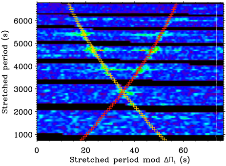
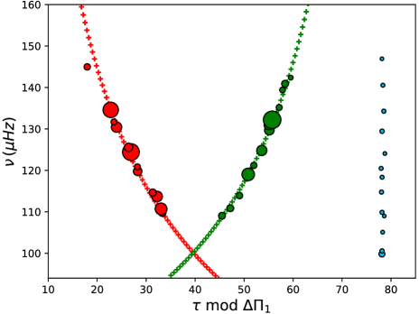
Figure 6: Stretched period échelle diagram for dipole gravity-dominated mixed modes. Top panel is the work led by co-author Appourchaux with $\Delta\Pi_{1}=76.3$ s. Fitted ridges with $m=\{-1,1\}$ are represented as red and orange crosses, respectively; while $m=0$ is represented as a continuous white line. The black stripes show the location of the $l=0,2$ mode power which has been removed for clarity. Bottom panel summarizes the finding of co-author Gehan, where peaks with a height-to-background ratio equal to or above 10 are represented. The symbol size varies as the measured power spectral density. Ridges with $m=\{-1,0,1\}$ are represented in green, light blue, and red, respectively. Red and green crosses represent the fit of the ridges with $m=\pm 1$. The location of the $m=0$ ridge is identified considering that the $m=0$ ridge is median with respect to $m=\pm 1$ ridges.

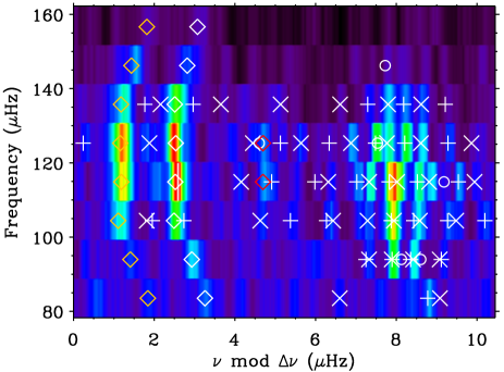
Figure 7: Peak-bagging results including mixed-mode analysis by co-author Appourchaux displayed in the form of an échelle diagram of the power spectrum for $\Delta\nu=$10.44 $\mu$Hz. Fitted frequencies are shown: $l=0$ white diamonds, $l=2$ orange diamonds, $l=3$ red diamonds, $l=1,m=-1$ white crosses, $l=1,m=0$ white circles, $l=1,m=+1$ white pluses.

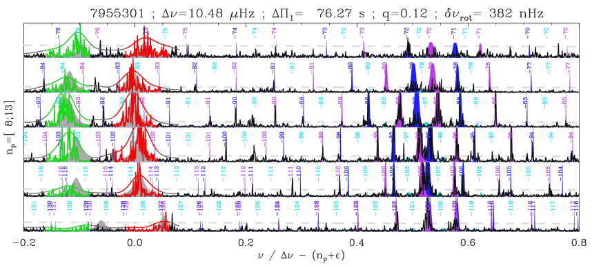
Figure 8: Peak-bagging results including mixed-mode analysis by co-author Mosser in the form of a line-by-line échelle diagram, for radial pressure orders 8 to 13. Radial and quadrupole modes are highlighted in red and green, respectively. The expected locations of dipole mixed modes are labelled with their mixed radial orders, and indicated with a color depending on the azimuthal order: dark blue ($m=-1$), light blue ($m=0$), or purple ($m=+1$). $\ell=3$ modes, not identified in this plot, are located near the abscissa 0.21. The gray dashed lines correspond to height-to-background ratios of 7 and 10.

Table 3: Global seismic parameters of the RG component.

Parameter		Gaulme	Appourchaux	Mosser	Gehan	Vrard
$\nu_{\mathrm{max}}$	[$\mu$Hz]	$124.9\pm 0.4$		$122.7\pm 24.1$	$122.5\pm 5.6$
$\Delta\nu$	[$\mu$Hz]	$10.49\pm 0.02$	$10.496\pm 0.011$	$10.48\pm 0.05$	$10.45\pm 0.27$
$\Delta\Pi_{1}$	[s]		$76.297\pm 0.003$	$76.27\pm 0.03$	$76.3\pm 0.1$	$76.09\pm 0.72$
$q$			$0.098\pm 0.002$	$0.120\pm 0.013$		$0.17\pm 0.05$
$\delta_{01}$			$0.027\pm 0.001$	$0.029\pm 0.006$
$\epsilon_{p}$			1.233	$1.194\pm 0.052$
$\epsilon_{g}$			$0.24\pm 0.005$	$0.246\pm 0.032$
$\nu_{\mathrm{core}}$	[nHz]		$382\pm 2$	$382\pm 10$	$380\pm 6$
$\nu_{\mathrm{env}}$	[nHz]		$39\pm 6$
$i$	[∘]		74.2${}^{+7.7}_{-14.1}$		$75.8^{+14.2}_{-6.6}$

4.2 Mixed modes

4.2.1 Formalism

As indicated in the introduction, the RG component of KIC 7955301 shows a rich spectrum of dipolar mixed pressure and gravity modes. Here we briefly summarize some basic properties of the mixed modes (see Mosser et al. 2015, and references therein). The frequency of the mixed modes is an implicit expression given by

$$\tan\theta_{p}=q\tan\theta_{g},$$ (3)

where $q$ is the coupling factor between the p and g modes, $\theta_{p}$ is the phase of the mixed modes with respect to the asymptotic p-mode frequencies separated by the large separation $\Delta\nu$, while $\theta_{g}$ the phase of the mixed modes with respect to the asymptotic g-mode periods separated by the period spacing $\Delta\Pi_{1}$. In other words,

$$\theta_{p}=\pi\left(\frac{\nu}{\Delta\nu}-\frac{1}{2}-\epsilon_{p}\right),$$ (4)

where $\nu$ is the mixed mode frequency and $\epsilon_{p}$ is a phase offset, and

$$\theta_{g}=\pi\left(\frac{P}{\Delta\Pi_{1}}-\epsilon_{g}\right),$$ (5)

where $P$ is the mixed mode period and $\epsilon_{g}$ is a gravity offset. Solving the implicit relation given by Eq. (3) provides the mixed mode frequencies.

The period separation $\Delta P$ between two consecutive mixed mode periods is given by

$$\Delta P=\zeta(\nu)\,\ \Pi_{1},$$ (6)

where $\zeta$ is related to the phases given above by

$$\zeta(\nu)=\left[1+\frac{\nu^{2}\Delta\Pi_{1}}{q\Delta\nu}\frac{\cos^{2}\theta_{g}}{\cos^{2}\theta_{p}}\right]^{-1}.$$ (7)

$\zeta$ is also useful for expressing the frequency splitting of these dipole modes $\delta\nu_{\rm rot}$, since we have

$$\delta\nu_{\mathrm{rot}}=\zeta(\nu)\delta\nu_{\mathrm{core}}+(1-\zeta(\nu))\,\delta\nu_{\mathrm{env}},$$ (8)

where $\delta\nu_{\mathrm{core}}$ is the rotation mainly sampled by the g modes, while $\delta\nu_{\mathrm{env}}$ is the rotation mainly sampled by the p modes. We stress that this expression is not symmetrical in terms of the azimuthal order $m$ since it depends on the mixed mixed frequency

$$\zeta(\nu+\delta\nu_{\mathrm{rot}})\neq\zeta(\nu-\delta\nu_{\mathrm{rot}}),$$ (9)

as discussed in Mosser et al. (2012).

Equations (3) and (8) provide a full description of the mode frequency and its associated rotational splitting. To ensure a robust analysis of the mixed modes, four independent studies were led by co-authors Appouchaux, Gehan, Mosser, and Vrard. All followed the approach developed by Mosser et al. (2015), where the first step consists of stretching the oscillation spectrum to transform the mixed-mode pattern into a comb-like pattern based on the gravity period spacing $\Delta\Pi_{1}$. Despite a common approach, each fitter performed different analysis with independent routines. The following subsections provide details for all.

4.2.2 Analysis adapted from Appourchaux (2020)

The stretched power spectrum is interpolated onto a regular grid for producing the échelle diagram of Fig. 6 (top panel). The fitted asymptotic frequencies of the multiplet of the dipole mixed modes are computed using the expressions of Mosser et al. (2015) where $\zeta$ is replaced by the analytical formulation given above. We note again that the mode splitting is not symmetrical due to $\zeta$ depending on frequency. First guesses for $\Delta\Pi_{1}$, rotation and $q$ are provided by the results of Mosser et al. (2014, 2015, 2017), respectively. These three parameters are then visually adjusted to obtain a figure similar to that of Fig. 6. The asymptotic frequencies obtained by this procedure are very close to the actual peaks, within $0.1\ \mu$Hz, easing the fitting of the peaks by Maximum Likelihood Estimation (MLE). Due to the dense forest of dipole mixed modes, the fitting window for these modes is $0.5\,\mu$Hz, while for $l=0,2$ and 3, it is 3 $\mu$Hz. Fitted frequencies are displayed in Table LABEL:tab:peak_bagging. The échelle diagram of the power spectrum with the fitted frequencies is shown on Fig. 7

In a second step, we determine all the parameters of the asymptotic expression of the dipole mode frequencies, i.e. $\Delta\Pi_{1}$, q, $\epsilon_{g}$, $\delta_{01}$, $\nu_{\mathrm{core}}$ and $\nu_{\mathrm{env}}$ by doing an unweighted least squares fit of the fitted frequencies. The optimization is performed by using the same algorithm as in Appourchaux (2020). Data were trimmed to exclude three frequencies out of the 62 dipole mode frequencies (see frequencies in Table LABEL:tab:peak_bagging). The root mean square value of the optimized difference is $0.00\pm 0.03$ $\mu$Hz. The error bars were then extracted by doing a Monte Carlo simulation using the error bars on the dipole mode frequencies extracted from MLE. The optimization was then repeated 100 times. The values obtained are reported in Table 3.

The inclination angle of the star was extracted using a single mixed mode (n=-94) for which the triplets was clearly fitted. We used the ratio between heights of modes with different azimuthal orders (Gizon & Solanki 2003). The ratio between the $m=0$ and the $m=\pm 1$ is 0.08${}^{+0.257}_{-0.060}$ providing an angle of $i=74.2^{+7.7}_{-14.1}$ degrees.

4.2.3 Analysis following Gehan et al. (2018)

Before the mixed-mode analysis, the frequency at maximum amplitude $\nu_{\mathrm{max}}$ was derived by using the FRA pipeline. It computes a smoothed power spectrum, then fits a Gaussian envelope accounting for oscillations along with a background contribution to measure $\nu_{\mathrm{max}}$. It also performs a likelihood ratio test to validate the measured $\nu_{\mathrm{max}}$ and check whether oscillations are present. The FRA pipeline was used in Huber et al. (2022) and is explained in detail in Gehan et al. (2022). The large spacing $\Delta\nu$ was measured by using the EACF.

The power spectrum was then stretched as in Mosser et al. (2015) and Gehan et al. (2018). Pressure-dominated mixed modes were located using the RG universal oscillation pattern (Mosser et al. 2011) and excluded, in order to keep only gravity-dominated modes that are mostly sensitive to the core rotation rate. The stretched period échelle diagram reveals that dipole gravity-dominated mixed modes line up along two ridges, associated with the azimuthal orders $m=\pm 1$ (Fig. 6, bottom). Fitting these ridges (Fig. 6) allows us to derive the mean core rotational splitting, which is found to be $\delta\nu_{\mathrm{rot,core}}=380\pm 6$ nHz (Gehan et al. 2018, for details). Once the azimuthal order of mixed modes is identified, we measure the inclination angle of the rotation axis from the ratio between heights of modes with different azimuthal orders (Gizon & Solanki 2003). Only the ridges with azimuthal orders $m=\pm 1$ are visible, but we know where to look for the missing $m=0$ ridge in the background, at the midpoint between the $m=+1$ and $m=-1$ ridges (Fig. 6, bottom). We obtain an inclination of $i=75.8^{+14.2}_{-6.6}$ degrees. We refer to Gehan et al. (2021) for the details of the inclination measurement procedure. We note that the maximal possible value according to the uncertainties is $i=90^{\circ}$, so that the star is possibly seen equator-on. This is because the $m=0$ ridge is lost in the background, thus there is a possibility that the peaks with $m=0$ are completely absent and that the observed signal is only due to background noise.

4.2.4 Analysis following Mosser et al. (2018)

Stretching the power spectrum first requires a precise fitting of the radial and quadrupole modes $l=0$ and 2, thanks to the RG universal oscillation pattern, in order to locate precisely the expected pure pressure dipole modes. Firstly, the modes with the largest height-to-background ratios (HBR) are used to determine the parameters of the fit. Secondly, we pick modes with lower HBRs, still larger than $5$, provided that they stick to the asymptotic pattern within a frequency range wide six times the spectral resolution. We applied the method of Mosser et al. (2018) for analyzing the rotational splittings to overcome the difficulties arising from the overlap of rotational multiplets larger than period spacings. The global seismic parameters derived from the fit of the mixed-mode pattern, following the updated approach described by Pinçon et al. (2019), are reported in Table 3. The frequency analysis is displayed in Fig. 8.

4.2.5 Analysis adapted from Vrard et al. (2016)

The steps that follow the power-spectrum stretching differ from the analysis led by co-author Mosser. We started by computing the Fourier transform of the stretched spectrum to obtain a first $\Delta\Pi_{1}$ value following the work of Vrard et al. (2016). After that, the coupling parameter $q$ was determined following the method described in Mosser et al. (2017), which involves searching for the maximum of the Fourier Transform of the stretched oscillation spectrum. Finally, an iterative process was performed between $\Delta\Pi_{1}$ and $q$: the $\Delta\Pi_{1}$ measurement was redone with the measured $q$ value, then the inverse is performed until the $\Delta\Pi_{1}$ and $q$ values converge. The final measurement of $\Delta\Pi_{1}$ and $q$ is obtained when those values converge. The final fitted parameters lead to $\Delta\Pi_{1}=76.09\pm 0.72$ for the gravity mode period spacing and $q=0.17\pm 0.05$ for the coupling parameter.

4.2.6 The big picture from the mixed mode analysis

The four independent approaches used to analyse the mixed dipole modes agree (Table 3). Firstly, the measured mixed-mode period spacing $\Delta\Pi_{1}\approx 76$ s associated with the large frequency p-mode spacing $\Delta\nu\approx 10.5\,\mu$Hz, definitely classifies the star as an RGB (Mosser et al. 2014). Secondly, the fact that the $m=0$ modes are not detected indicates a large inclination angle $i$ of the RG rotation axis with respect to the line of sight. The two authors who carefully analysed the ratio of the amplitudes of the mixed $m=1$ to $m=0$ dipole modes report a very consistent inclination angle of $\approx 75^{\circ}$, with a rather large uncertainty ranging from $60^{\circ}$ to $90^{\circ}$. Thirdly, according to Mosser et al. (2012, Eqs., 22 and 23), the frequency spacing measured on the mixed modes provides a proxy of the mean core rotation period with the relation $P_{\mathrm{core}}\approx 1/2\delta\nu_{\mathrm{core}}=15.1\pm 0.2$ days by assuming an uncertainty of 5 nHz on $\delta\nu_{\mathrm{core}}$. The average splitting of the envelope determined by co-author Appourchaux is about 10 times smaller, leading to a mean rotation period of $148_{-20}^{+27}$ days. If we add the fact that no spot-related variability was measured from the Kepler lightcurve and that the oscillation amplitude meet our expectations for that type of RG, we can safely conclude that the RG is a regular slow rotator that does not exhibit any sign of tidally increased spin.

5 Dynamical model

The combined photodynamical analysis of the Kepler photometry, the eclipse timing variations of the inner binary, and the radial-velocity curve of the outer giant component offer a robust dynamical determination of the mass of the RG ($M_{\mathrm{A}}$) and of the total mass of the inner binary ($M_{\mathrm{bin}}$). It can be seen as follows. The amplitude of the RV curve gives the spectroscopic mass function:

$$f(M_{\mathrm{bin}})=M_{\mathrm{bin}}\left(\frac{q_{\mathrm{out}}}{1+q_{\mathrm{out}}}\right)^{2}\sin^{3}i_{\mathrm{out}},$$ (10)

where $q_{\mathrm{out}}=M_{\mathrm{bin}}/M_{\mathrm{A}}$ and $i_{\mathrm{out}}$ are the mass ratio and the inclination of the outer (or wide) binary formed by the RG and the center of mass of the inner eclipsing pair. In addition, Borkovits et al. (2016) showed that the ETV of the eclipsing binary is strongly dominated by the gravitational three-body perturbations against the pure light-travel time effect. Detailed analytical investigations of third-body perturbed ETVs (Borkovits et al. 2011, 2016) have shown that such curves tightly constrain almost all of the orbital elements of both the inner and outer orbits, together with the mutual inclination of the two orbital planes. Their amplitude is related to the outer mass ratio as

$$\mathcal{A}_{\mathrm{dyn}}\propto\frac{1}{1+q_{\mathrm{out}}}.$$ (11)

Finally, the variation of the eclipse depth and duration of the inner eclipsing binary offer a very precise determination of the varying inclination of both the inner orbit of the eclipsing pair and the outer orbit.

The combined photodynamical analysis was carried out with the software package Lightcurvefactory (see, e. g. Borkovits et al. 2019, and further references therein). This code contains a built-in numerical integrator to calculate the three-body perturbed coordinates and velocities of the three bodies, a multi-band light curve, ETV and RV curve emulators, and an MCMC-based parameter search routine for the inverse problem. The latter employs an implementation of the generic Metropolis-Hastings algorithm (see e. g. Ford 2005).

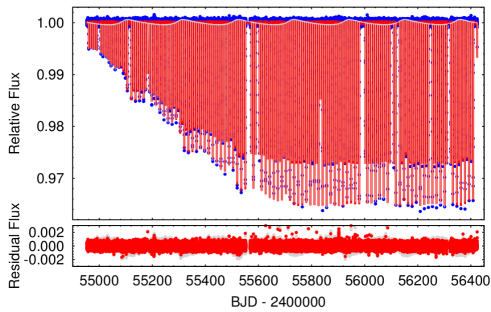
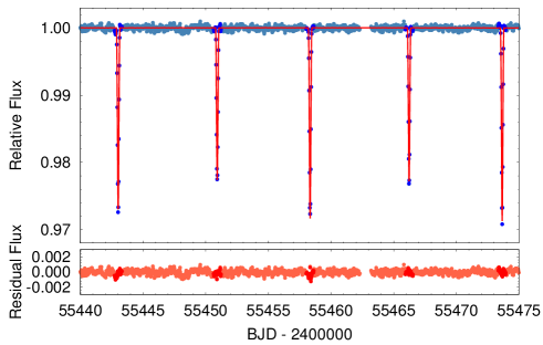
Figure 9: The long cadence Kepler lightcurve of KIC 7955301 together with the joint photodynamical model lightcurve solution. Upper left panel: The complete Q0-Q17 lightcurve (blue) with the bestfitted solution (red). This solution was obtained with the negligation of the Doppler-boosting effect. The grey curve show the same model after ‘switching on’ the Doppler-boosting. While this effect, in theory, should have been observable with the accuracy of Kepler photometry, the reasons of its negligence is discussed in the text. Upper right panel: A 1-month-long section of the Kepler observations overplotted with the photodynamical solution. The pale blue circles represent each individual observations but, for the analysis only dark blue data (located within the $\pm 0\aas@@fstack{p}02$ phase environment of each eclipses) were considered. Lower panels show the residual data.

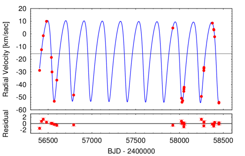
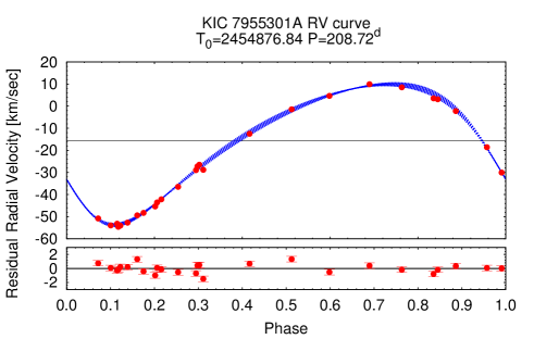
Figure 10: Left: radial velocity data (red) as a function of time expressed in modified Julian dates, with their best fit model (blue line). Right: radial-velocity data (red) folded over the RG orbital period as a function of the orbital phase. The dispersion of the best-fit curve in blue is caused by the varying shape of the RV curve as a function of time.

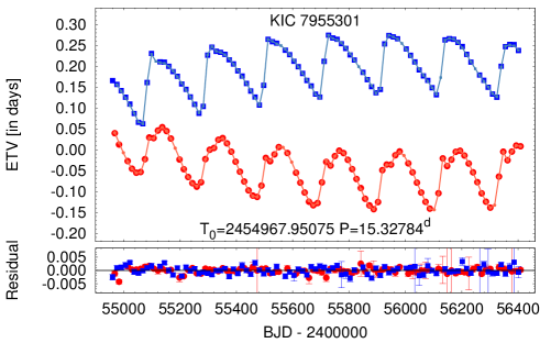
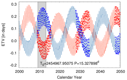
Figure 11: The eclipse timing variations of KIC 7955301 on different timescales: Observations vs model and predictions. Left: The primary and secondary ETV curves derived from Kepler-observations (red circles and blue boxes, respectively), together with the photodynamical model solution (smaller, pale red and blue symbols, connected with straight lines, respectively). Right: ETV-like curves derived from the times of the inferior and superior conjunctions of the secondary of the inner pair (pale red and blue lines), overplotted with ‘true’, forecasted primary and secondary ETV points (larger red and blue symbols) during the eclipsing phases of the inner binary for the first half of the present century. The dynamically forced short-period apsidal motion of the inner binary is nicely visible. The grey-shaded area stands for the interval of the Kepler-measurements.

Table 4: Orbital and astrophysical parameters of KIC 7955301 from the joint photodynamical lightcurve, RV and ETV solution with and without the involvement of the stellar energy distribution and PARSEC isochrone fitting.

	without SED+PARSEC			with SED+PARSEC
orbital elements
	subsystem
	Ba–Bb		A–B	Ba–Bb		A–B
$P$ [days]	$15.31831_{-0.00025}^{+0.00024}$		$209.760_{-0.020}^{+0.020}$	$15.31825_{-0.00023}^{+0.00023}$		$209.761_{-0.018}^{+0.018}$
$a$ [R⊙]	$31.68_{-0.11}^{+0.19}$		$217.0_{-0.9}^{+1.4}$	$31.68_{-0.08}^{+0.11}$		$216.9_{-0.5}^{+1.1}$
$e$	$0.02763_{-0.00015}^{+0.00012}$		$0.2733_{-0.0014}^{+0.0013}$	$0.02757_{-0.00007}^{+0.00007}$		$0.2737_{-0.0014}^{+0.0013}$
$\omega$ [deg]	$295.80_{-0.20}^{+0.22}$		$117.02_{-0.40}^{+0.39}$	$295.90_{-0.19}^{+0.18}$		$116.99_{-0.39}^{+0.39}$
$i$ [deg]	$87.757_{-0.039}^{+0.037}$		$84.23_{-0.25}^{+0.25}$	$87.768_{-0.038}^{+0.034}$		$84.40_{-0.32}^{+0.23}$
$\tau$ [BJD - 2400000]	$54961.5184_{-0.0083}^{+0.0090}$		$54876.85_{-0.12}^{+0.12}$	$54961.5225_{-0.0081}^{+0.0076}$		$54876.84_{-0.11}^{+0.12}$
$\Omega$ [deg]	$0.0$		$-5.28_{-0.17}^{+0.16}$	$0.0$		$-5.19_{-0.17}^{+0.16}$
$i_{\mathrm{m}}$ [deg]	$6.34_{-0.24}^{+0.26}$			$6.18_{-0.23}^{+0.29}$
$\omega^{\mathrm{dyn}}$ [deg]	$239.7_{-1.4}^{+1.1}$		$240.6_{-1.4}^{+1.2}$	$239.2_{-1.4}^{+1.4}$		$239.9_{-1.4}^{+1.5}$
$i^{\mathrm{dyn}}$ [deg]	$5.36_{-0.21}^{+0.23}$		$0.97_{-0.04}^{+0.04}$	$5.23_{-0.20}^{+0.25}$		$0.95_{-0.04}^{+0.04}$
$\Omega^{\mathrm{dyn}}$ [deg]	$236.4_{-1.1}^{+1.3}$		$56.4_{-1.1}^{+1.3}$	$236.9_{-1.4}^{+1.4}$		$56.9_{-1.4}^{+1.4}$
$i_{\mathrm{inv}}$ [deg]	$84.77_{-0.22}^{+0.21}$			$84.91_{-0.27}^{+0.20}$
$\Omega_{\mathrm{inv}}$ [deg]	$-4.47_{-0.15}^{+0.14}$			$-4.39_{-0.14}^{+0.13}$
mass ratio $[q=M_{\mathrm{sec}}/M_{\mathrm{pri}}]$	$0.929_{-0.009}^{+0.010}$		$1.399_{-0.012}^{+0.010}$	$0.933_{-0.003}^{+0.003}$		$1.406_{-0.013}^{+0.010}$
$K_{\mathrm{pri}}$ [km s-1]	$50.44_{-0.32}^{+0.37}$		$31.61_{-0.12}^{+0.13}$	$50.53_{-0.16}^{+0.13}$		$31.65_{-0.08}^{+0.08}$
$K_{\mathrm{sec}}$ [km s-1]	$54.27_{-0.38}^{+0.46}$		$22.58_{-0.16}^{+0.23}$	$54.13_{-0.16}^{+0.24}$		$22.50_{-0.10}^{+0.23}$
$\gamma$ [km s-1]	$-15.779_{-0.048}^{+0.050}$			$-15.769_{-0.036}^{+0.036}$
stellar parameters
	Ba	Bb	A	Ba	Bb	A
Relative quantities
fractional radius [$R/a$]	$0.0285_{-0.0005}^{+0.0004}$	$0.0256_{-0.0007}^{+0.0006}$	$0.0241_{-0.0005}^{+0.0008}$	$0.0285_{-0.0002}^{+0.0002}$	$0.0259_{-0.0001}^{+0.0001}$	$0.0263_{-0.0006}^{+0.0008}$
fractional flux [in $Kepler$-band]
Physical Quantities
$M$ [$M_{\odot}$]	$0.941_{-0.011}^{+0.020}$	$0.876_{-0.011}^{+0.012}$	$1.298_{-0.019}^{+0.030}$	$0.939_{-0.007}^{+0.011}$	$0.877_{-0.008}^{+0.013}$	$1.292_{-0.010}^{+0.026}$
$R$ [$R_{\odot}$]	$0.903_{-0.014}^{+0.012}$	$0.809_{-0.022}^{+0.022}$	$5.22_{-0.12}^{+0.22}$	$0.901_{-0.007}^{+0.010}$	$0.822_{-0.006}^{+0.006}$	$5.70_{-0.13}^{+0.20}$
$T_{\mathrm{eff}}$ [K]	$5372_{-46}^{+84}$	$5138_{-48}^{+73}$	$4800$	$5580_{-70}^{+44}$	$5313_{-62}^{+38}$	$4804_{-48}^{+26}$
$L_{\mathrm{bol}}$ [L⊙]	$0.611_{-0.035}^{+0.043}$	$0.408_{-0.026}^{+0.034}$	$13.00_{-0.58}^{+1.12}$	$0.704_{-0.038}^{+0.038}$	$0.480_{-0.022}^{+0.022}$	$15.55_{-0.75}^{+0.87}$
$M_{\mathrm{bol}}$	$5.27_{-0.07}^{+0.06}$	$5.71_{-0.09}^{+0.07}$	$1.95_{-0.09}^{+0.05}$	$5.15_{-0.06}^{+0.06}$	$5.57_{-0.05}^{+0.05}$	$1.79_{-0.06}^{+0.05}$
$M_{V}$	$5.45_{-0.09}^{+0.08}$	$5.97_{-0.12}^{+0.08}$	$2.36_{-0.09}^{+0.05}$	$5.24_{-0.07}^{+0.07}$	$5.73_{-0.06}^{+0.07}$	$2.15_{-0.05}^{+0.06}$
$\log g$ [dex]	$4.503_{-0.014}^{+0.014}$	$4.565_{-0.019}^{+0.024}$	$3.115_{-0.026}^{+0.017}$	$4.500_{-0.005}^{+0.004}$	$4.551_{-0.003}^{+0.003}$	$3.034_{-0.023}^{+0.019}$
$\log$(age) [dex]	$-$			$9.65_{-0.03}^{+0.02}$
$[\mathrm{M/H}]$ [dex]	$-$			$0.061_{-0.037}^{+0.028}$
$E(B-V)$ [mag]	$-$			$0.09_{-0.02}^{+0.02}$
$(M_{V})_{\mathrm{tot}}$	$2.26_{-0.09}^{+0.05}$			$2.05_{-0.05}^{+0.07}$
distance [pc]	$-$			$1369_{-29}^{+44}$

We simultaneously analysed the eclipse photometry from the Kepler light curve, the primary and secondary ETVs deduced from the same light curve, and the RVs of the outer RG component. For the Kepler-light curve, we only used the $\phi\pm 0\aas@@fstack{p}02$ phase sections of each eclipses to reduce computational costs. Except for preliminary tests, the following parameters were adjusted with MCMC:

• Nine of the twelve orbital parameters. Regarding the inner orbit of the eclipsing pair, we fit $e_{1}\cos\omega_{1}$, $e_{1}\sin\omega_{1}$, and $i_{1}$, where $e_{1}$ is the osculating eccentricity, $\omega_{1}$ the argument of periastron and $i_{1}$ the orbital inclination. About the wide outer orbit, besides $e_{2}\cos\omega_{2}$, $e_{2}\sin\omega_{2}$, and $i_{2}$, we fit the anomalistic period $P_{2}$, the periastron passage time $\tau_{2}$ and the longitude of the node $\Omega_{2}$. Regarding two of the three “missing” parameters describing the inner orbit, namely, the period $P_{1}$ and time of a primary eclipse or, with other words, the time of an inferior conjunction of the secondary component of the inner pair $\mathcal{T}^{\mathrm{inf}}_{1}$, they were constrained internally at each trial step via the ETV curves in the manner described in Borkovits et al. (2019). Finally, the third “missing” orbital parameter, the longitude of the node of the inner orbit $\Omega_{1}$ was set to zero. It can be done because, for the complete analysis, only the difference of the nodes, i. e. $\Delta\Omega=\Omega_{2}-\Omega_{1}$ has relevance. Therefore, in such a manner, by setting $\Omega_{2}$, one sets $\Delta\Omega$. Note that because the motion of the three stars are not purely Keplerian, none of the orbital parameters is constant. Therefore, all the trial values either adjusted, constrained, or fixed in the initializing phase of any trial steps refer only a given epoch $t_{0}$.

• Three parameters connected to the masses of the three stars: the RG mass $M_{\mathrm{A}}$, the spectroscopic mass function $f(M_{\mathrm{B}})$, and the mass ratio of the eclipsing binary $q_{1}=M_{\mathrm{Bb}}/M_{\mathrm{Ba}}$.

• Four parameters almost exclusively connected to the light curve. The first is the duration of the primary eclipse around the epoch $t_{0}$ ($\Delta t_{\mathrm{pri}}$), which is related to the sum of the fractional radii of the members of the inner eclipsing binary, that is, the radius divided by the semi major axis. The second is the ratio of the stellar radii of the inner pair $R_{\mathrm{Bb}}/R_{\mathrm{Ba}}$. The third is the RG radius $R_{\mathrm{A}}$. The fourth is the ratio of the effective temperatures of the eclipsing pair $T_{\mathrm{Bb}}/T_{\mathrm{Ba}}$. We note that in case of a single-band photometric observations, the EB lightcurve only carries information about the temperature ratio – most strictly speaking, the passband-dependent surface brightness ratio – of the two components rather than their true temperatures. Therefore, one of the temperatures should be taken from some external sources. In a single binary it can be obtained from spectroscopic analysis or from stellar energy distribution (SED) data (see, e. g. Miller et al. 2020). In the present situation, most of the total flux comes from the third RG component which makes the classical approach to be irrelevant. Therefore, we assume that the two components of the inner binary are still on the main sequence, by being less massive than the RG, so that at each trial step the software sets the effective temperature of the primary component of the eclipsing pair $T_{\mathrm{Ba}}$ accordingly to the mass – radius and mass – effective temperature relations of Tout et al. (1996) for main sequence stars. About the RG component, we assume that its contribution to the light curve is only a constant extra flux. Therefore, we fixed its temperature to $T_{\mathrm{A}}=4\,800$ K for all runs. In such a way, adjusting the RG radius $R_{\mathrm{A}}$ directly sets its bolometric luminosity, and indirectly its total flux in the Kepler photometric band. Hence, the adjustment of $R_{\mathrm{A}}$ was simply used to set the amount of the extra flux to the eclipsing binary light curve or; in other terms, it served as a substitute of the usual third light parameter.

Regarding other smaller effects that are mainly light-curve related, we used a logarithmic limb-darkening law. The corresponding parameters were calculated internally at each trial step with the use of the publicly available passband-dependent tables of the Phoebe software (Prša & Zwitter 2005). For the well detached nature of both the inner and the outer binaries and, therefore, for the practically spherical shape of the stars, the gravity darkening coefficients have no detectable effect on the light curve solution. Therefore, we did not consider the results of the recent, more sophisticated study of Claret & Bloemen (2011), but simply adopted the fixed value of $g=0.32$, which is based on the seminal model of Lucy (1967). Finally, we neglected both the reradiation/illumination and the Doppler-boosting effects (Loeb & Gaudi 2003; van Kerkwijk et al. 2010). While the first effect has really no any influence on the light curve of our system, this is not certainly true for the second one. In this regard, we note that, as one can see in the left panel of Fig. 9, Doppler-boosting would result in an $\sim 1000$ ppm amplitude variation in the out-of-eclipse flux level with the period of the outer orbit, which, in theory, should be detected with Kepler. Despite this fact, it cannot be seen in the lightcurves, because this low amplitude variation, having period longer than two quarters was filtered out during the data processing, which fact justifies its negligence in the analysis.

The median values of the orbital and physical parameters of the triple system derived from the MCMC posteriors and their 1-$\sigma$ uncertainties are tabulated in Table 4. The observed versus model photometric, RV, and ETV curves are plotted in Figs. 9–11.

6 Stellar evolution model

We modeled the system in three independent manners by using parameters that are deduced from the observations. The first two model the RG component only, by considering the seismic information and atmospheric parameters. The first method (PARAM) makes use of the asteroseismic global parameters $\nu_{\mathrm{max}}$, $\Delta\nu$, and $\Delta\Pi_{1}$ to optimize the model from a grid of stellar evolution models. The second method makes use of the individual frequencies of the radial modes and $\Delta\Pi_{1}$. The third method is a complete model of the triple system, which includes both the RG and the inner binary, but that does not make use of the asteroseismic constraints.

6.1 Red-giant model based on the global seismic parameters

We used the code PARAM (Rodrigues et al. 2017) to infer the radius, mass, and age of the RG component by using a combination of seismic and non-seismic constraints. On the one hand, the average large frequency separation is computed using the radial-mode frequencies of the models in the grid, not added as an a-posteriori correction to the scaling relation between $\Delta\nu$ and the square root of the stellar mean density. On the other hand, $\nu_{\mathrm{max}}$ in the model grid is computed using a simple scaling relation (Kjeldsen & Bedding 1995), by considering $\nu_{\mathrm{max,\odot}}=3090\,\mu Hz$. The period spacing can also be included in the list of seismic constraints, in which case it is compared with the asymptotic value of $\Delta\Pi_{1}$ coming out of the models (see Rodrigues et al. 2017). The grid of stellar evolution models used in PARAM is the same as the reference grid adopted in Khan et al. (2019) and Miglio et al. (2021) (G2).

We used the individual radial-mode frequencies in Table LABEL:tab:peak_bagging to compute an average $\Delta\nu$ that can be directly compared with that from the model grid, and obtain a value ($\Delta\nu=10.48$) compatible with that obtained using the EACF (see Sec. 4). With the observational constraints $\Delta\nu$, $\nu_{\mathrm{max}}$, $T_{\mathrm{eff}}$, and [M/H] we obtain $R_{\mathrm{A}}=5.84\pm 0.09\,R_{\odot}$, $M_{\mathrm{A}}=1.27\pm 0.05\,M_{\odot}$, and an age of $4.9\pm 0.9$ Gyr. In Fig. 12 we show the posterior probability density function (PDF) of radius, mass and age, compared with the same resulting from the asteroseismic modeling based on individual frequencies that is exposed in the next section (Sect. 6.2).

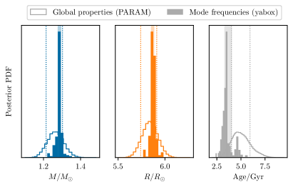
Figure 12: Mass, radius and age posterior probability distribution functions derived from seismic constraints. Empty histograms show the distributions obtained using PARAM, and the dotted lines show their associated $\pm 1\sigma$ credible regions. Solid histograms and shaded regions indicate the same quantities obtained using the individual mode frequencies.

6.2 Red-giant model based on the oscillation frequencies

We generated models using the MESA code (Paxton et al. 2011, 2013, 2015, 2018, 2019) with diffusion and settling of heavy elements, with no core overshoot, no mass loss, using an Eddington-grey atmosphere, and with chemical abundances evaluated relative to the solar values of Grevesse & Sauval (1998).

The nonradial mixed modes in red giants can be described as combinations of pure p- and g-modes — or ”$\pi$” and ”$\gamma$-modes”, in the sense of Aizenman et al. (1977). We evaluate these pure $\pi$- and $\gamma$-mode frequencies using the modified wave operator construction described in Ong & Basu (2020), which splits the standard wave operator into two complementary p- and g-mode wave operators, each supporting only one type of wave propagation. We solve for these mode frequencies numerically with the pulsation code GYRE (Townsend & Teitler 2013). The observed p-dominated mixed modes of degree $l\geq 2$ in red giants are very well approximated as pure $\pi$-modes, and as such we match the model $\pi$-modes against the observed modes of degree $l\geq 2$. Likewise, dipole modes far from the p-dominated mixed modes have period spacings close to those of the pure $\gamma$-modes; accordingly, rather than evaluating $\Delta\Pi_{1}$ using its asymptotic value, we compute it directly from the pure dipole $\gamma$-modes.

The mode frequencies returned from stellar models are known to be systematically offset from those which would be obtained from stars of identical interior structure, owing to systematic errors in the modeling of stellar surfaces — this is referred to as the asteroseismic ”surface term”. As such, the model frequencies cannot be used directly to construct likelihood functions against the observed mode frequencies in the usual fashion. Instead, we use a nonparametric description — “$\epsilon$-matching”, via the algorithm of Roxburgh (2016) — to characterize the discrepancy between the model and observed mode frequencies in a surface-independent fashion. For this purpose we use only the model $l=0,2,3$ frequencies, since those modes which we observe are either radial p-modes, or can be approximated as being entirely p-dominated; here we use the mode frequencies reported by co-author Appourchaux. For the dipole modes, which are more strongly mixed, we used the period spacing only, also as reported by co-author Appourchaux. Since the g-mode cavity is well-localized into the stellar interior, no surface correction is needed.

To supplement these seismic constraints, we used the spectroscopic constraints from scenario C ([M/H] and $T_{\mathrm{eff}}$). These were used to compute log-likelihood functions as

$$\chi^{2}=\chi^{2}_{\mathrm{spec}}+\left(\chi^{2}_{\epsilon}+\chi^{2}_{\Delta\Pi_{1}}\right)/f,$$ (12)

where $f$ is initially set to 1 when performing the optimization. Optimization was performed using the differential-evolution algorithm as implemented in the yabox package (Mier 2017), using the initial mass $M$, initial helium and metal mass fractions $Y_{i}$ and $Z_{i}$, and the mixing-length efficiency parameter $\alpha_{\text{MLT}}$ as the independent variables for this optimization. After the optimization was complete, $f$ is set to the minimum value of $\chi^{2}_{\mathrm{seis}}$ along the optimization trajectory, in order to ensure that the reported results are not entirely dominated by the seismic quantities, which are significantly more precisely constrained than the spectroscopic ones.

We may consider the optimization trajectory to yield a series of nonuniformly distributed samples of the likelihood function over the input parameter space. As such, if we were to report estimates of stellar properties by naively taking likelihood-weighted averages of the desired quantities over all the sampled points, or find posterior distributions by constructing likelihood-weighted histograms, we would be over-representing parts of the parameter space where the density of samples is high to begin with. Effectively, the sampling function of the optimization trajectory provides an implicit prior distribution, which we estimate using a Gaussian kernel density estimator and divide out to yield a nonuniformly sampled posterior distribution function assuming a uniform prior. Using this uniform-prior posterior distribution, we report the posterior median and $\pm 1\sigma$ quantiles of the following of fundamental stellar properties:

$$M_{\mathrm{A}} = 1.281^{+0.015}_{-0.004}\,M_{\odot}$$ (13)

$$R_{\mathrm{A}} = 5.863^{+0.024}_{-0.011}\,R_{\odot}$$ (14)

$$Y_{i} = 0.291^{+0.010}_{-0.013}$$ (15)

$$Z_{i} = 0.012^{+0.003}_{-0.001}$$ (16)

$$\alpha_{\mathrm{MLT}} = 1.87^{+0.05}_{-0.09}$$ (17)

$$\rho = 0.0089^{+0.00003}_{-0.00003}\,\mbox{g cm}^{-3}$$ (18)

$$\mathrm{age} = 3.43^{+0.62}_{-0.16}\mbox{Gyr}$$ (19)

We compare these results with those obtained with the PARAM code, by plotting the posterior distributions of the mass, radius and age in Fig. 12. The mass and radius appear to be in agreement with the values obtained from only $\Delta\nu$, $\nu_{\mathrm{max}}$, and $\Delta\Pi_{1}$ with the PARAM routine, while the ages are somewhat different although still within the $1\sigma$ error. We discuss this difference in Sect. 7.2.

6.3 Overall system model based on classical parameters

We have compared the classical parameters of the three components of the system with the isochrones and tracks from the YaPSI database (Spada et al. 2017); the results are summarized in Figure 13. In the two panels on the left of the Figure, the measured masses and radii are compared with several isochrones of appropriate metallicity, generated by interpolation from the YaPSI database. The best fit is obtained for an age of $4.5\pm 0.2$ Gyr for the primary component (top left panel); the components of the inner binary are marginally compatible with this isochrone (bottom left). In the right panel of Figure 13, we show the best-fitting isochrone, together with evolutionary tracks constructed with the same code and input physics used for the YaPSI models (see Spada et al. 2017 for details). For the primary star, both the isochrone and the track are in good agreement with the observed radius and luminosity (note that the isochrone and track for component A essentially coincide on the RGB, as a result of the fast-paced evolution typical of this evolutionary phase). The agreement is less good for the two components of the inner binary. This could be ascribed to non-standard effects not taken into account in our models.

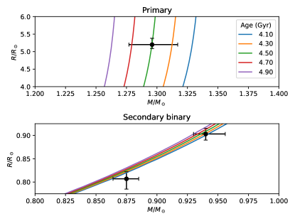
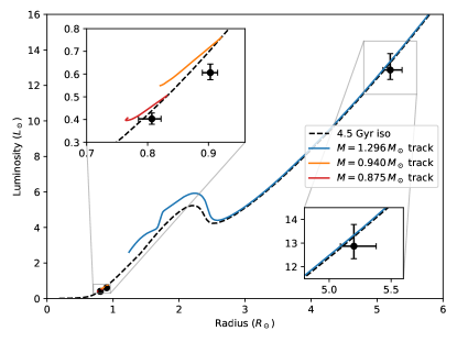
Figure 13: Visual fit of observed classical parameters of the system with theoretical tracks and isochrones from the YaPSI database (Spada et al. 2017). Left: comparison in the mass radius plane with isochrones of different ages for the primary (top panel), and the two components of the inner binary (bottom). Right: comparison in the radius-luminosity plane; a 4.5-Gyr isochrone and evolutionary tracks of appropriate mass and metallicity are shown.

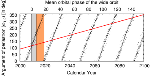
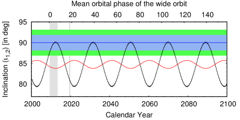
Figure 14: The evolutions of some of the orbital elements on a century-long timescale, obtained via numerical integrations. Left: The variations of the observable arguments of periastrons ($\omega_{1,2}$) of the inner and outer orbits (black and red, respectively). The dynamically forced apsidal motions of both orbits are well visible. The grey and orange shaded regions mark the intervals of the Kepler and the ground-based spectroscopic follow up observations, respectively. Right: The inclinations of the inner and outer binaries (black and red curves, respectively). The green- and lightblue-shaded horizontal areas denote the inclination domains of the inner and outer orbits where eclipses can occur. The vertical grey area represents the domain of the Kepler-observations, while the thin, black, vertical line denotes the interval of the 27-day-long TESS observations (Sector 14). As one can see, during these measurements the inner inclination ($i_{1}$) was far below the green line, therefore, the inner pair did not present any eclipses. (Note, the dark blue line simply stands for $i_{1,2}=90\degr$ to guide the eye.)

Figure 15: Photodynamical model light curve of KIC 7955301 for the present century. The $\sim 19.2$ yr-period precession cycle is clearly visible. Within a cycle the inner pair exhibits regular eclipses during a $\sim 7.3$ yr-long interval. The last eclipsing session has been finished at 2nd January 2016 with a short, $\sim 80$ ppm amplitude fading, while the next session is expected to begin at 18 January 2028. The grey vertical area represents the time of Kepler observations, and TESS Sector 14 observations are also denoted with a thin vertical line.

6.4 Model based on isochrones and SED

We carried out a second spectro-photodynamical study with the software package Lightcurvefactory that includes the lightcurve, ETVs and RVs, as earlier, but also the stellar energy distribution (SED), a stellar evolution code (PARSEC, Bressan et al. 2012), and the Gaia-based accurate trigonometric distance. The cumulative SED, which consists of pass-band magnitudes, drives the temperature of sources, or at least of the dominant one. That way, effective temperatures together with stellar masses and radii determine the locations of the stars on co-eval PARSEC evolutionary tracks. Besides the lightcurve, RVs, and ETVs, the publicly available multipassband magnitudes (see Table LABEL:tbl:mags) were simultaneously fitted against the theoretical passband magnitudes interpolated from theoretical PARSEC isochrone tables. We refer the reader to Borkovits et al. (2020) for a detailed description of the method.

With this new model, the free parameters partially differ from Sect. 5. Firstly, three new free parameters are added: the logarithm of the age; the metallicity $[M/H]$ of the system; the interstellar extinction $E(B-V)$. Furthermore, the distance of the system is constrained a posteriori at each trial step, by minimizing the value of $\chi^{2}_{\mathrm{SED}}$. Secondly, the stellar radii and temperatures that used to be free are no longer fitted. However, the code computes them internally by interpolating the appropriate PARSEC tables according to the trial values of the [mass, age, metallicity] triplets at each trial runs. The results are tabulated in the last columns of Table 4.

The comparison of the results from the purely dynamical analysis, which is independent from stellar evolution models, and the analysis including dynamical analysis, SED, and isochrones, produce output parameters that lie within their 1-$\sigma$ uncertainties. This means that the inclusion of stellar evolution models into the complex analysis did not lead to any unavoided bias in the values of the physical properties of the system. It also means that our model-independent lightcurve solution has led to dimensionless quantities, like fractional radii and temperature ratios, that are fully consistent with stellar evolutionary models.

The mass of the RG component $M_{\mathrm{A}}=1.30^{+0.03}_{-0.02}\,M_{\odot}$ is in excellent agreement with the asteroseismic analysis. The inner binary components appear to be on the main sequence with masses $M_{\mathrm{Ba}}=0.94_{-0.01}^{+0.02}\,\mathrm{M}_{\odot}$, $M_{\mathrm{Bb}}=0.88\pm 0.01\,\mathrm{M}_{\odot}$, and radii of $R_{\mathrm{Ba}}=0.90\pm 0.01\,\mathrm{R}_{\odot}$, $R_{\mathrm{Bb}}=0.81\pm 0.02\,\mathrm{R}_{\odot}$ in both solutions.

In contrast, the radius of the RG component $R_{\mathrm{A}}$ and the temperatures $T_{\mathrm{Ba}}$, $T_{\mathrm{Bb}}$ of the inner stars differ by about $5-10\%$ between the two models. This is expected because these quantities are not functions of the lightcurve properties and of the dynamics of the system. Only the ratio of the effective temperatures of the inner binary $T_{\mathrm{Bb}}/T_{\mathrm{Ba}}$ is model-independent; this one is in good agreement (within $1\%$) between the two models. In the purely dynamical model (Sect. 5), the RG temperature was fixed to the available catalog value $T_{\mathrm{A}}=4800$ K. Here, the combined dynamical, SED and isochrone model confirms this value by finding $T_{\mathrm{A}}=4804_{-48}^{+26}$ K, which within the uncertainty of the value we measured from the disentangled optical spectra (Table 2). In the dynamical model, the temperature $T_{\mathrm{Ba}}$ of the primary star of the EB was internally set with the use of the zero age main sequence mass-radius and mass-luminosity relations of Tout et al. (1996), and the temperature ratio $T_{\mathrm{Bb}}/T_{\mathrm{Ba}}$ was an adjustable parameter. In the combined model they were constrained from the appropriate PARSEC isochrone. This latter model has resulted in higher temperatures by $\sim 200$ K in accordance with the fact that KIC 7955301 is a quite old system, having an age of $4.5\pm 0.2$ Gyr according to the present model. Finally, the combined model predicts the RG radius to be of $R_{\mathrm{A}}=5.70_{-0.13}^{+0.20}\,\mathrm{R}_{\odot}$, which is in agreement with the asteroseismic value.

The stellar metallicity $[M/H]=0.06_{-0.04}^{+0.03}$ and interstellar extinction $E(B-V)=0.09\pm 0.02$ obtained from the combined model are consistent with catalog values (see Table LABEL:tbl:mags). Finally, the SED fitting provides an estimate of the photometric distance of $d=1369_{-29}^{+44}$ pc, which is in perfect agreement with trigonometric distance of $d=1375\pm 35$ pc derived from the Gaia EDR3 catalog by Bailer-Jones et al. (2021). However, we keep in mind that Gaia EDR3 data are not corrected for binarity and, might suffer from systematic errors for such a triple system.

About the dynamical evolution of the system, the small outer-to-inner period ratio $P_{2}/P_{1}\approx 13.8$ puts the system among the category of compact hierarchical triple systems. That being said, the small mutual inclination of $i_{\mathrm{m}}=6\aas@@fstack{\circ}2\pm 0\aas@@fstack{\circ}3$ and almost circular inner orbit ($e_{1}=0.0276\pm 0.0001$), the orbital configuration of the system is stable in dynamical timescale. Consequently, the dynamical evolution of the system will be driven by the stellar evolution of the evolved RG component. Therefore, here we restrict our discussion for some short term effects, and their observational consequences.

In Fig. 14 we plot the variations of the observable arguments of periastrons ($\omega_{1,2}$) and inclinations ($i_{1,2}$) of the inner and outer orbits during the present century. The very fast, dynamically forced apsidal motion can nicely be seen on the ETV curves determined from the 4-yr-long Kepler-observations (see Fig. 11). An observationally more dramatic effect caused by precession of the orbital plane of the inner binary is illustrated in Fig. 15. As the orbital plane precesses with a half amplitude of $i^{\mathrm{dyn}}_{1}=5\aas@@fstack{\circ}3\pm 0\aas@@fstack{\circ}2$ around the invariable plane of the triple (having an inclination of $i_{\mathrm{inv}}=84\aas@@fstack{\circ}8\pm 0\aas@@fstack{\circ}3$) with a period of $P_{\mathrm{node}}\approx 19.2$ yr, the inner binary exhibits eclipses (with varying eclipse depths) during a $\approx 7.3$ yr-long interval, while in the remaining $\approx 11.9$ yr the system no longer exhibits eclipses. Fortunately, Kepler observations caught the first half of the latest eclipsing session and it led to the discovery of this very exciting system. This eclipsing session has ended at the very beginning of 2016, and KIC 7955301 will no exhibit any eclipses till the first days of 2028. In accordance with our findings, TESS spacecraft did not observe any remarkable light variations of this target when the original Kepler-field was revisited three times from 2019 to 2022 (Fig. 16).

7 Concluding discussion

7.1 Dynamical versus seismic masses

With this paper, we illustrate the first detailed analysis of a hierarchical triple system that includes an oscillating RG by combining asteroseismology, spectroscopy and dynamical measurements. This system is an important benchmark for calibrating the measurement of RG masses with asteroseismology. Thanks to the acquisition of 23 high-resolution spectra with the ARCES spectrometer at APO we were able to first classify the system as an SB1 and monitor the RV shift of the RG component along its orbit. Then, with the dynamical model solution, we could disentangle and co-add the optical spectra to derive the atmospheric parameters of the three components, even though the parameters of the inner binary have a low S/N. By fixing the RG surface gravity to that found by the complete Lightcurvefactory model, we were able to determine the RG temperature and metallicity at $T_{\mathrm{A}}=4720\pm 105$ K and [M/H]$=-0.01\pm 0.12$ (Table 2).

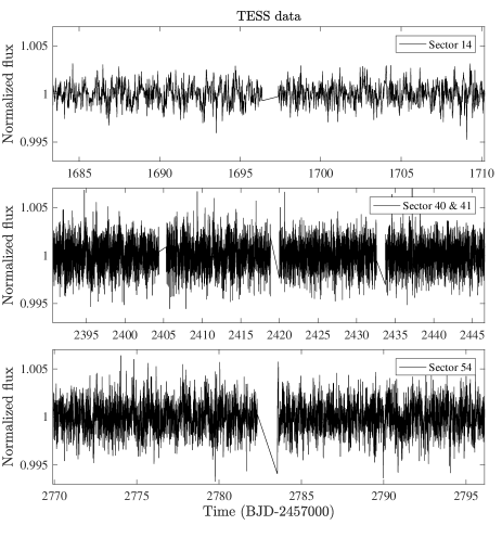
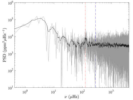
Figure 16: TESS observations of KIC 7955301 from 2019 to 2022. Top panel: time series processed with the software package FITSH (Pál 2012). Bottom panel: power spectral density of the times series for sector 14 only. The vertical red dot-dashed line indicates $\nu_{\mathrm{max}}$ and the vertical blue dashed line indicates Kepler’s Nyquist frequency.

We computed the asteroseismic mass of the RG in three different manners. The first and most basic one, which consists of applying the asteroseismic scaling law (SL) tuned for RG stars by Mosser et al. (2013) from the values of $\nu_{\mathrm{max}}$, $\Delta\nu$, and $T_{\mathrm{A}}$, leads to $M_{\mathrm{A,SL}}=1.27\pm 0.05\ M_{\odot}$. The second makes use of the (PARAM) approach that fits the global asteroseismic parameters, including $\Delta\Pi_{1}$, and by including the metallicity on a grid of stellar-evolution models. The mass appears to be the exact same as with the asteroseismic scaling relation: $M_{\mathrm{A,\texttt{PARAM}}}=1.27\pm 0.05\,M_{\odot}$. Finally, the most sophisticated approach based on fitting individual oscillation frequencies leads to a mass of $M_{\mathrm{A}}=1.281^{+0.015}_{-0.004}\,M_{\odot}$.

The RG mass that we derive from the purely dynamical modeling – independent from both asteroseismology and stellar evolution models – is $1.30^{+0.03}_{-0.02}\,M_{\odot}$. The uncertainty is thus about 2 %, which is better than what can be obtained from asteroseismology or stellar evolution models based on atmospheric parameters, luminosity and parallaxes. This type of system, a solar-like oscillator in an SB1 hierarchical triple system, should definitely be considered for helping to calibrate the asteroseismic masses. About ten of them are available in Gaulme et al. (2013) and Gaulme & Guzik (2019), even though none of them exhibit such clear ETVs, which means that a 2 % accuracy on mass may not be achievable with those.

It is interesting to notice that in this system the asteroseismic mass matches the dynamical one, contrary to what was observed with most RGs in EBs (Gaulme et al. 2016; Brogaard et al. 2018; Benbakoura et al. 2021), where asteroseismology appeared to overestimate masses by about 15 % on average. This puzzling fact may just be a case that the sample of RG oscillators with accurate independent mass estimates is small and the dispersion of the observed overestimation is large, but it could also highlight issues with RGs in EBs where the companion is a MS dwarf star. For an RG in an EB, the mass of the RG is driven by the low S/N Doppler shift that is measured by tracking the absorption lines of the companion star. In most cases, the flux coming from the companion is less than 5 % of the total flux. We also note that a good agreement between dynamical and seismic masses was found with the double RG KIC 9246715 (Rawls et al. 2016), where there were no issues of noisy RVs.

In contrast, KIC 7955301 is a special target with respect to the bulk of RGs in EBs because it is the least evolved and thus smallest RG ($\approx 5.85\,R_{\odot}$) for which we have an independent mass measurement. The radii of all of the RGs in EBs listed in Benbakoura et al. (2021), for example, range from 8 to $14R_{\odot}$. In addition a significant fraction of them are red clump stars. So far, no significant overestimation of stellar masses and radii by asteroseismology was observed for MS and subgiant stars. We may have an intermediate case here, for which asteroseismic measurements are unbiased. To clarify the question, our recommendation is to take new RV measurements of the RG/EBs listed in Benbakoura et al. (2021) and Gaulme & Guzik (2019) with larger S/N ratios, that is longer exposure times, and with spectrometers that are dedicated to high-precision RV measurements.

7.2 Age of the system

One of the goals of the future ESA PLATO mission (Rauer et al. 2014) is to provide ages of solar-like MS stars hosting exoplanets with an accuracy of 10 %. Many papers dealing with stellar physics report ages arising from stellar evolution codes with a similar precision, especially when asteroseismic measurements are available. With this paper, we could have run a single stellar evolution code and provided an age with a relatively low uncertainty. We decided to let four different modelers estimate the age in an independent fashion. We obtain $4.9\pm 0.9$ Gyr with PARAM, $3.43^{+0.62}_{-0.16}$ Gyr with MESA, $4.5\pm 0.2$ Gyr with YaPSI, and $4.5\pm 0.2$ Gyr with Lightcurvefactory, that is 18.4, 22.7, 4.4, and 4.4 % respectively. Both the YaPSI and Lightcurvefactory estimates have a better precision likely because the three components of the system are included into the optimization process. Ages determined for the RG only (component A), with the help of asteroseismic and classical parameters, have uncertainties of about 20 %, despite RGs are usually considered to be good cases for age estimate thanks to their fast evolution along the RG branch.

Our age estimate thus ranges from 3.3 to 5.8 Gyr, which is quite broad given the unusually vast amount of information that we have. By looking more closely, the age is consistent between the three “standard” approaches that use the classical parameters (mass, metallicity, effective temperature), and the global asteroseismic parameters (PARAM only). On the contrary, the model based on reproducing the individual oscillation frequencies with MESA stands apart. Even though a deeper understanding of the differences between the age estimates goes beyond the scope of the paper, we can already draw some conclusions. A careful inspection of the posterior probability distribution (PDF) of the mass, radius and age (Fig. 12) shows a good agreement between the mass and radius obtained with PARAM and MESA, whereas the age PDF appears to be bimodal with MESA. In fact, the secondary peak of the age distribution matches the PARAM estimate (at $\approx 4.5$ Gyr). A key aspect of the MESA-model based optimization is that the helium abundance $Y$ and metallicity $Z$ are two free independent parameters of the model. The resulting $Y$ value of 0.29 is quite large by considering the slightly sub-solar value found for the metallicity ($Z\approx 0.012$) and assuming a linear $Y=Y(Z)$ relation, and that the Sun falls on that relation (see Fig A.4 Miglio et al. 2021). A difference of about 0.02 in $Y$ with respect to what we have in the grid used in PARAM, would mean a difference of $\sim 15\,\%$ in age which, considering also the slight difference in mass, could explain the different age estimate.

7.3 Formation of the system

Physical properties and orbital configuration carry information about the formation process of the systems. We refer the reader to Borkovits et al. (2022) and references therein, where a connection between dynamical and orbital parameters and formation scenarios is discussed. An outer eccentricity of 0.27 for a 209-day period outer orbit is far from being exceptional. For example, Borkovits et al. (2016) reported 16 triple star candidates with smaller outer period than that of KIC 7955301 and, 6 of them have larger outer eccentricities. Since then, further highly eccentric systems amongst substantially more compact triply eclipsing triples were found in TESS data (Borkovits et al. 2022).

With an outer semi-major axis less than 10 AU, KIC 7955302 is considered to be a compact triple system. The formation of such type of systems involves either a fragmentation of the accretion disk, or a disk-mediated capture of the outer component. In both cases the outer star forms by being less massive than the inner binary. Then, thanks to its wider and eccentric orbit it sweeps out a larger orbit and thus accretes most of the infalling material from the accretion disk, which eventually leads $q_{\mathrm{out}}$ toward larger values. Although it is expected that the total mass of the inner pair remains larger than the mass of the wide component by the end of the complete formation process, the third component may actually become the most massive star of the system (Tokovinin 2021), which is the case of KIC 7955301.

7.4 Evolution of the system

In the short term, we have shown that the inner binary components eclipse each other over a period of about 7.3 years, and stop eclipsing for the next 11.9 years. The RG will never eclipse the inner binary as seen from the Earth. This is why we were able to study the eclipses of the inner binary from the Kepler data and that we are not able to do so with TESS. The eclipses should be visible again during the ESA PLATO mission, whose nominal operations should happen between 2027 and 2031. The PLATO observations will certainly help fine-tune the model of the system.

Over the long term and in general, stars are likely to merge in close multiple-star systems when the most massive component reaches the tip of the RG branch. This is especially true for low-mass stars that ignite helium only at the tip of the red giant branch, after reaching very large radii ($\sim 200\ R_{\odot}$). RGs may swallow planets or stars, converting their orbital momentum into spin and friction loss. There is indirect observational evidence for it. For example, about 3 % of the solar-mass stars on the red-giant branch and 11 % of the helium-burning stars observed by Kepler display unusually fast rotation and magnetic fields (e.g., Tayar et al. 2015; Ceillier et al. 2017; Tayar & Pinsonneault 2018; Gaulme et al. 2020). This means that a fraction of the RGs in that mass range gains angular momentum between the RGB and the RC. Until alternative explanations are provided, a likely possibility is that these stars have engulfed a stellar or substellar companion. Recently, Price-Whelan et al. (2020) reported a notable dearth of close companions around the red clump – where companions may have been engulfed when the primary star ascended the upper giant branch – in the color-magnitude diagram produced by the APO Galactic Evolution Experiment (APOGEE, Majewski et al. 2017), which is part of the Sloan Digital Sky Survey IV (e.g., Blanton et al. 2017). The orbital configuration of KIC 7955301 represents a borderline case for this type of scenario. The current distance at periastron between the giant and the inner binary is about $\approx 142\,R_{\odot}$ according to the data from Table 4.

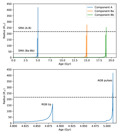
Figure 17: Top panel: radius evolution of the three components according to the MIST tracks (with masses and metallicity set equal to their nominal values from Table 4). The semi-major axis of the inner binary is indicated by the black dotted line, and the semi-major axis of the outer orbit with dashed lines. Bottom panel: zoom on the RG component around its RGB and AGB phases.

We can formulate some broad predictions for the long-term evolution of the system, assuming that the dynamical interaction among the components can be neglected until they come into contact with each other because of post-MS evolution. Figure 17 shows the evolution of the radii of the three components according to evolutionary tracks generated with the MIST web interpolator (Choi et al. 2016), setting the masses to the central values given in Table 4 (1.29, 0.94, and 0.88 $M_{\odot}$ for components A, Ba, and Bb, respectively), and the metallicity to +0.06. Significant mass loss takes place during the RGB and AGB phases, and as a result all three stars reach a final mass of about $0.5\,M_{\odot}$ by the end of their respective AGB phases. Stellar rotation is not included in these models. At an age of approximately 5 Gyr, component A (already a red giant at present time) reaches the RGB tip, and shortly after (relative to the $10^{9}$ yr time scale) the AGB tip and thermal pulses phase. The peak radius reached at the tip of the RGB ($\approx 160\,R_{\odot}$) is mostly equal to the distance at periastron, while the peak radius on some of the AGB pulses is significantly larger than the semi-major axis of the outer orbit, and thus merging can be expected to occur at one of those times. Should merging of component A with the inner binary be avoided because of some process not considered in this crude analysis, at around 15 Gyr component Ba will evolve onto the RGB and merge with Bb. In the light of this discussion, it is comforting that none of our age estimates is larger than 5 Gyr.

Appendix A Radial velocity data

Table 5 contains the radial velocities obtained at Apache Point and Haute-Provence observatories.

Table 5: Radial velocity data obtained at Apache Point and Haute-Provence observatories.

Date	RV
(KJD)	km s-1
1569.823526	-28.82
1591.832861	-12.50
1611.826703	-1.44
1648.831533	9.92
1704.641327	-18.59
1711.645679	-30.04
1737.619563	-53.19
1766.572107	-36.50
1958.878300	-48.28
3090.825370	4.65
3189.617802	-50.82
3195.587236	-53.95
3203.595970	-52.70
3216.717021	-45.36
3217.631558	-43.57
3219.657836	-42.14
3416.917213	-49.39
3444.847760	-28.94
3445.534184⋆	-27.26
3446.421966⋆	-26.49
3542.669669	8.53
3557.755987	3.53
3559.754443	3.12
3568.344058⋆	-2.24
3616.635254	-54.58
3617.597411	-54.06

Appendix B Oscillation frequencies

Table LABEL:tab:peak_bagging displays the oscillation frequencies of the RG component, as performed by co-authors Appourchaux and Mosser. 1]

Table 6: Oscillation frequencies of KIC 7955301 by co-authors Appourchaux and Mosser (COR method). The columns report $\nu_{\mathrm{as}}$ as asymptotic fit ($\mu$Hz); $\nu_{\mathrm{obs}}$ are the observed peak ($\mu$Hz) with uncertainties; $nm$ is the proxy of the mixed order ($nm=np-ng$ ; 0 for p-modes); zeta = zeta factor of mixed modes (Mosser+2015, 2018), and HBR is the height-to-background ratio).

					Appourchaux		Mosser
$l$	$m$	$n$	$nm_{\mathrm{TA}}$	$nm_{\mathrm{BM}}$	$\nu_{\mathrm{obs,TA}}$	err	$\nu_{\mathrm{obs,BM}}$	err	$\nu_{\mathrm{as}}$	$\zeta$	HBR
					$\mu$Hz	$\mu$Hz	$\mu$Hz	$\mu$Hz	$\mu$Hz
0	0	7	8	87	0.057	…	…	…	…	…	…
0	0	8	9	0	96.918	0.027	96.905	0.063	96.593	0.000	17.4
0	0	9	10	0	106.921	0.009	106.917	0.009	106.920	0.000	47.4
0	0	10	11	0	117.396	0.013	117.402	0.018	117.323	0.000	110.2
0	0	11	12	0	127.851	0.167	127.753	0.013	127.802	0.000	127.9
0	0	12	13	0	138.268	0.018	138.230	0.027	138.357	0.000	50.2
0	0	13	14	0	149.021	0.004	148.943	0.013	148.987	0.000	21.1
0	0	14	15	…	159.718	0.059	…	…	…	…	…
1	-1	…	-136	…	90.142	0.002	…	…	…	…	…
1	1	…	-132	…	92.323	0.022	…	…	…	…	…
1	-1	…	-132	…	92.626	0.052	…	…	…	…	…
1	1	8	…	-126	…	…	98.377	0.014	98.371	0.989	5.4
1	1	8	-120	…	101.235	0.004	…	…	…	…	…
1	-1	8	-120	-121	101.310	0.004	101.305	0.017	101.277	0.825	19.5
1	-1	8	-119	-120	101.874	0.006	101.880	0.026	101.831	0.614	64.9
1	1	8	-119	…	101.881	0.006	…	…	…	…	…
1	0	8	-119	…	102.112	0.001	…	…	…	…	…
1	1	8	-118	…	102.342	0.015	…	…	…	…	…
1	-1	8	-118	-119	102.401	0.006	102.391	0.011	102.390	0.825	14.5
1	-1	8	-117	…	103.061	0.002	…	…	…	…	…
1	1	8	-117	…	103.103	0.005	…	…	…	…	…
1	1	8	…	-118	…	…	103.840	0.014	103.853	0.973	7.3
1	-1	…	-113	…	106.245	0.000	…	…	…	…	…
1	1	…	-113	…	106.384	0.009	…	…	…	…	…
1	1	…	-112	…	107.164	0.012	…	…	…	…	…
1	-1	9	-110	-111	109.059	0.001	109.051	0.012	109.066	0.985	14.1
1	1	9	-109	-111	109.807	0.002	109.806	0.010	109.816	0.977	20.5
1	1	9	-108	-110	110.698	0.001	110.696	0.010	110.705	0.949	24.2
1	-1	9	-108	-109	110.863	0.002	110.837	0.021	110.868	0.938	5.6
1	1	9	…	-109	…	…	111.554	0.012	111.550	0.823	10.6
1	-1	9	-107	-108	111.717	0.001	111.719	0.016	111.693	0.770	34.8
1	1	9	-107	-108	112.305	0.013	112.254	0.035	112.188	0.567	59.1
1	-1	9	-106	-107	112.369	0.016	112.325	0.016	112.299	0.584	59.3
1	0	9	-118	-107	102.592	0.001	112.514	0.021	112.547	0.699	9.2
1	1	9	-106	-107	112.862	0.004	112.876	0.022	112.836	0.822	34.9
1	-1	9	-105	-106	113.013	0.011	113.041	0.016	113.014	0.870	26.1
1	1	9	-105	-106	113.699	0.010	113.703	0.012	113.718	0.949	20.3
1	-1	9	-104	-105	113.913	0.007	113.931	0.011	113.933	0.959	9.1
1	1	9	-104	-105	114.624	0.002	114.655	0.013	114.673	0.976	15.8
1	-1	9	…	-103	…	…	115.938	0.014	115.914	0.986	45.1
1	1	9	…	-103	…	…	116.647	0.017	116.668	0.988	6.1
1	-1	10	…	-102	…	…	116.953	0.011	116.941	0.988	14.6
1	-1	10	…	-101	…	…	117.977	0.015	117.988	0.988	5.2
1	1	10	…	-101	…	…	118.717	0.018	118.741	0.986	5.4
1	-1	10	-99	-100	119.028	0.002	119.032	0.013	119.051	0.984	31.0
1	1	10	-99	-100	119.782	0.002	119.779	0.015	119.801	0.978	9.1
1	-1	10	…	-99	…	…	120.157	0.019	120.127	0.974	9.3
1	1	10	-98	-99	120.854	0.003	120.858	0.010	120.864	0.954	21.1
1	-1	10	-97	-98	121.186	0.008	121.180	0.015	121.199	0.935	7.1
1	0	10	…	-98	…	…	121.558	0.014	121.549	0.899	6.3
1	1	10	-97	-98	121.893	0.004	121.897	0.011	121.881	0.831	94.6
1	-1	10	-96	-97	122.198	0.004	122.196	0.015	122.170	0.717	110.0
1	0	10	…	-97	…	…	122.385	0.020	122.417	0.586	25.2
1	1	10	-96	-97	122.695	0.007	122.708	0.044	122.622	0.523	275.3
1	-1	10	-95	…	122.891	0.009	…	…	…	…	…
1	0	10	…	-96	…	…	123.030	0.027	123.078	0.707	15.7
1	1	10	-95	-96	123.394	0.000	123.384	0.012	123.369	0.823	45.7
1	-1	10	-94	-95	123.685	0.022	123.723	0.009	123.721	0.897	35.3
1	0	10	-94	-95	124.054	0.006	124.054	0.013	124.069	0.933	14.4
1	1	10	-94	-95	124.409	0.001	124.416	0.010	124.430	0.953	72.8
1	-1	10	-93	-94	124.812	0.001	124.809	0.015	124.834	0.966	28.1
1	0	10	…	-94	…	…	125.187	0.017	125.204	0.973	5.1
1	1	10	-93	-94	125.555	0.007	125.557	0.014	125.577	0.978	15.7
1	-1	10	…	-93	…	…	125.982	0.018	126.011	0.981	10.8
1	-1	10	-91	-92	127.197	0.002	127.194	0.016	127.221	0.986	30.5
1	0	10	…	-92	…	…	127.627	0.017	127.598	0.986	40.7
1	1	11	…	-91	…	…	129.217	0.010	129.209	0.983	16.2
1	-1	11	-89	-90	129.760	0.051	129.689	0.015	129.714	0.980	28.7
1	0	11	-89	…	129.919	0.000	…	…	…	…	…
1	1	11	-89	-90	130.442	0.002	130.437	0.014	130.460	0.972	33.4
1	-1	11	-88	-89	130.954	0.005	130.957	0.016	130.982	0.961	16.4
1	1	11	-88	-89	131.653	0.026	131.697	0.012	131.704	0.924	9.5
1	-1	11	-87	-88	132.191	0.001	132.193	0.013	132.212	0.854	101.6
1	0	11	-87	-88	132.850	0.024	132.531	0.015	132.518	0.760	7.4
1	1	11	-87	-88	132.800	0.009	132.807	0.014	132.785	0.628	114.0
1	-1	11	-86	-87	133.083	0.017	133.051	0.025	133.095	0.486	27.4
1	0	11	…	-87	…	…	133.137	0.075	133.286	0.509	22.9
1	1	11	-86	-87	133.524	0.030	133.523	0.017	133.494	0.613	71.9
1	-1	11	-85	-86	133.923	0.001	133.924	0.010	133.934	0.811	101.8
1	1	11	-85	-86	134.598	0.003	134.593	0.011	134.608	0.923	66.9
1	-1	11	-84	-85	135.179	0.004	135.176	0.014	135.191	0.955	9.3
1	1	11	…	-85	…	…	135.924	0.010	135.928	0.972	11.9
1	1	…	-83	…	137.527	0.003	…	…	…	…	…
1	-1	…	-82	…	137.917	0.409	…	…	…	…	…
1	1	12	-82	-83	138.722	0.003	138.718	0.014	138.733	0.983	8.5
1	-1	12	-81	-82	139.410	0.004	139.411	0.015	139.432	0.982	12.3
1	-1	12	-80	-81	140.891	0.002	140.890	0.012	140.905	0.970	18.0
1	0	12	…	-81	…	…	141.292	0.016	141.274	0.963	6.1
1	-1	12	-79	-80	142.366	0.007	142.362	0.014	142.356	0.906	5.7
1	1	12	-79	-80	143.050	0.024	142.984	0.018	143.008	0.770	8.7
1	-1	12	-78	-79	143.555	0.099	143.527	0.014	143.515	0.512	18.1
1	0	12	…	-79	…	…	143.527	0.087	143.698	0.447	18.1
1	1	12	-78	-79	143.940	0.003	143.882	0.013	143.874	0.469	21.5
1	-1	12	-77	-78	144.373	0.001	144.362	0.011	144.351	0.719	26.7
1	0	12	…	-78	…	…	144.661	0.014	144.643	0.820	14.1
1	1	12	-77	-78	144.972	0.002	144.968	0.012	144.963	0.882	8.9
1	-1	12	…	-76	…	…	147.329	0.013	147.339	0.976	7.8
1	1	12	…	-76	…	…	148.101	0.013	148.086	0.980	11.5
1	0	13	…	-75	…	…	149.337	0.019	149.362	0.981	5.0
1	1	13	…	-75	…	…	149.754	0.014	149.736	0.980	8.8
1	0	13	…	-74	…	…	151.029	0.015	151.044	0.972	6.1
1	1	13	…	-74	…	…	151.407	0.013	151.415	0.968	7.5
1	-1	13	…	-72	…	…	153.902	0.017	153.879	0.647	13.8
1	0	13	-71	-72	153.925	0.010	154.185	0.046	154.102	0.518	5.8
1	1	13	…	-72	…	…	154.398	0.060	154.283	0.431	7.9
1	-1	13	…	-71	…	…	154.823	0.040	154.750	0.539	7.8
1	0	13	…	-71	…	…	155.020	0.026	154.979	0.666	5.6
1	1	13	…	-71	…	…	155.272	0.018	155.254	0.779	5.1
2	0	6	7	…	85.387	0.120	…	…	…	…	…
2	0	7	8	0	95.395	0.036	95.449	0.135	94.778	0.000	8.4
2	0	8	9	0	105.537	0.026	105.579	0.095	105.106	0.000	14.0
2	0	9	10	0	116.058	0.004	116.072	0.112	115.512	0.000	95.1
2	0	10	11	0	126.474	0.018	126.462	0.095	125.988	0.000	68.9
2	0	11	12	0	136.935	0.028	136.986	0.089	136.544	0.000	34.0
2	0	12	13	0	147.637	0.035	147.676	0.102	147.170	0.000	22.7
2	0	13	14	…	158.462	0.099	…	…	…	…	…
3	0	9	9	…	119.568	0.098	…	…	…	…	…
3	0	10	10	…	130.013	0.026	…	…	…	…	…

Table 6: Continued.

Appendix C Eclipse properties

Table LABEL:tab:eclipse_ppties presents the eclipses properties obtained with the Lightcurvefactory.

1]

Table 7: Eclipse properties.

n	$t_{1}$	$O_{1}-nP-t_{0}$	$D_{1}$	$W_{1}$	$t_{2}$	$O_{2}-nP-t_{0}$	$D_{2}$	$W_{2}$
	(KJD)	day	%	hour	(KJD)	day	%	hour
8	127.4560	4.4034	-0.55	2.10	134.9905	11.9379	-0.50	2.24
9	142.8022	4.3911	-0.52	2.15	150.3368	11.9121	-0.51	2.20
10	158.1280	4.3778	-0.53	2.32	…	…	…	…
11	174.1688	4.3612	-0.62	2.48	181.7034	11.8727	-0.66	2.18
12	188.7792	4.3464	-0.65	2.38	196.3137	11.8560	-0.72	2.39
13	204.1046	4.3251	-0.77	2.31	211.6391	11.8481	-0.88	2.53
14	219.4298	4.3058	-0.84	2.40	226.9644	11.8495	-0.96	2.57
15	235.7970	4.3025	-0.87	2.40	243.3315	11.8809	-0.91	2.48
16	250.0798	4.4026	-0.89	2.43	257.6144	11.9343	-1.01	2.57
17	265.4046	4.4707	-1.15	2.67	272.9391	11.9343	-1.39	2.78
18	…	…	…	…	288.2638	11.9523	-1.56	2.69
19	296.0539	4.4538	-1.38	2.67	303.5884	11.9615	-1.62	2.71
20	311.3988	4.4533	-1.38	2.79	318.9334	11.9532	-1.58	2.80
21	327.9493	4.4437	-1.40	2.79	335.4839	11.9355	-1.53	2.81
22	342.0480	4.4350	-1.35	2.71	…	…	…	…
23	357.3727	4.4217	-1.42	2.63	364.9072	11.8882	-1.68	2.79
24	372.6975	4.4051	-1.39	2.55	380.2320	11.8657	-1.71	2.70
25	388.7172	4.3921	-1.52	2.81	396.2517	11.8462	-1.81	2.79
26	405.2275	4.3752	-1.60	2.75	412.7621	11.8327	-1.93	2.87
27	418.6730	4.3593	-1.64	2.70	426.2075	11.8260	-2.04	2.79
28	433.9985	4.3395	-1.75	2.65	441.5330	11.8378	-1.98	2.78
29	449.3241	4.3562	-1.68	2.73	456.8586	11.8931	-1.94	2.95
30	464.6703	4.4809	-1.73	2.74	472.2048	11.9169	-2.15	2.94
31	480.6909	4.5004	-1.97	2.85	488.2254	11.9218	-2.52	2.98
32	495.3219	4.4902	-2.16	2.88	502.8565	11.9427	-2.58	2.93
33	510.6478	4.4881	-2.15	2.79	518.1823	11.9468	-2.53	2.92
34	525.9735	4.4836	-2.15	2.80	533.5081	11.9353	-2.61	2.85
35	541.2992	4.4736	-2.10	2.81	548.8337	11.9158	-2.50	2.93
36	556.6248	4.4625	-2.13	2.79	564.1593	11.8930	-2.54	2.85
37	571.9502	4.4480	-2.11	2.81	579.4847	11.8694	-2.63	2.90
38	587.2755	4.4327	-2.21	2.79	594.8100	11.8469	-2.72	2.88
39	602.6006	4.4184	-2.26	2.82	610.1351	11.8267	-2.79	2.91
40	617.9255	4.4025	-2.34	2.82	625.4601	11.8149	-2.88	2.98
41	633.2504	4.3860	-2.35	2.82	640.7849	11.8126	-2.94	2.85
42	648.5955	4.3689	-2.40	2.78	656.1300	11.8403	-2.81	2.87
43	663.9201	4.4192	-2.28	2.77	671.4546	11.9076	-2.86	2.85
44	679.2446	4.5282	-2.46	2.82	686.7792	11.9015	-3.18	2.86
45	694.5692	4.5233	-2.60	2.87	702.1037	11.9192	-3.28	2.84
46	709.8938	4.5202	-2.61	2.83	717.4283	11.9373	-3.21	2.83
47	…	…	…	…	…	…	…	…
48	740.5432	4.5077	-2.61	2.83	748.0777	11.9246	-3.15	2.85
49	755.8682	4.4959	-2.57	2.83	…	…	…	…
50	771.1933	4.4826	-2.66	2.77	778.7278	11.8789	-3.26	2.86
51	786.5186	4.4682	-2.60	2.81	794.0531	11.8559	-3.27	2.83
52	801.8440	4.4541	-2.64	2.82	809.3786	11.8329	-3.30	2.86
53	817.1901	4.4394	-2.68	2.80	824.7246	11.8117	-3.26	2.82
54	832.5158	4.4247	-2.68	2.88	840.0503	11.8028	-3.35	2.82
55	847.8416	4.4062	-2.67	2.85	855.3761	11.8107	-3.34	2.85
56	863.1674	4.3991	-2.65	2.81	870.7020	11.8615	-3.31	2.84
57	878.4933	4.4867	-2.63	2.79	886.0278	11.9122	-3.37	2.82
58	893.8191	4.5508	-2.71	2.83	901.3536	11.9018	-3.52	2.82
59	909.1448	4.5441	-2.71	2.83	916.6793	11.9259	-3.40	2.80
60	924.4703	4.5415	-2.71	2.83	932.0049	11.9388	-3.46	2.78
61	939.7958	4.5342	-2.72	2.85	947.3303	11.9356	-3.36	2.83
62	955.1211	4.5223	-2.72	2.78	962.6557	11.9193	-3.40	2.78
63	970.4463	4.5100	-2.63	2.66	977.9808	11.8984	-3.42	2.79
64	985.7713	4.4957	-2.73	2.77	993.3058	11.8751	-3.40	2.80
65	…	…	…	…	1008.6307	11.8528	-3.60	2.87
66	1016.4413	4.4668	-2.79	2.83	1023.9758	11.8293	-3.54	2.78
67	1031.7659	4.4523	-2.74	2.79	1039.3004	11.8137	-3.44	2.78
68	1047.0905	4.4373	-2.75	2.85	1054.6250	11.8063	-3.44	2.79
69	1062.4150	4.4218	-2.71	2.86	1069.9495	11.8256	-3.51	2.78
70	1077.7396	4.4325	-2.60	2.78	1085.2741	11.9016	-3.38	2.81
71	1093.0642	4.5402	-2.74	2.80	1100.5987	11.9150	-3.39	2.83
72	1108.3889	4.5620	-2.70	2.88	1115.9235	11.9160	-3.42	2.85
73	1123.7138	4.5594	-2.70	2.78	1131.2484	11.9406	-3.36	2.83
74	1139.0389	4.5551	-2.74	2.85	1146.5734	11.9484	-3.48	2.78
75	…	…	…	…	…	…	…	…
76	1169.7100	4.5329	-2.74	2.82	1177.2446	11.9232	-3.41	2.79
77	1185.0356	4.5174	-2.71	2.83	1192.5701	11.9026	-3.45	2.77
78	1200.3613	4.5009	-2.71	2.81	1207.8958	11.8782	-3.48	2.82
79	1215.6870	4.4898	-2.61	2.64	1223.2216	11.8551	-3.42	2.83
80	1231.0129	4.4730	-2.66	2.83	1238.5474	11.8341	-3.45	2.78
81	1246.3387	4.4609	-2.68	2.85	1253.8732	11.8182	-3.38	2.76
82	1261.6645	4.4451	-2.77	2.91	…	…	…	…
83	1276.9903	4.4303	-2.79	2.83	1284.5248	11.8558	-3.42	2.72
84	…	…	…	…	1299.8504	11.9417	-3.43	2.72
85	1307.6414	4.5621	-2.64	2.90	1315.1759	11.9248	-3.34	2.83
86	1322.9667	4.5669	-2.66	2.96	1330.5013	11.9406	-3.40	2.75
87	1338.2920	4.5667	-2.74	2.87	1345.8265	11.9605	-3.44	2.75
88	1353.6170	4.5586	-2.74	2.83	1361.1515	11.9625	-3.41	2.75
89	1368.9623	4.5468	-2.74	2.85	1376.4969	11.9525	-3.62	2.77
90	1384.2871	4.5313	-2.83	2.85	1391.8216	11.9353	-3.55	2.70
91	1399.6117	4.5150	-2.82	2.79	1407.1463	11.9131	-3.55	2.75
92	…	…	…	…	1422.4708	11.8905	-3.43	2.74
93	1430.2608	4.4844	-2.72	2.84	1437.7954	11.8663	-3.43	2.76
94	1445.5854	4.4706	-2.73	2.86	1453.1199	11.8456	-3.43	2.78
95	1460.9100	4.4564	-2.71	2.91	1468.4445	11.8321	-3.41	2.73
96	1476.5208	4.4392	-2.71	2.89	1484.0553	11.9078	-3.43	2.70
97	…	…	…	…	…	…	…	…
98	1506.9050	4.5093	-2.77	2.85	1514.4395	11.9682	-3.47	2.78
99	1522.2302	4.5590	-2.73	2.92	1529.7647	11.9494	-3.47	2.75
100	1537.5556	4.5621	-2.64	2.94	1545.0901	11.9717	-3.49	2.77
101	1552.8811	4.5624	-2.69	2.90	1560.4156	11.9858	-3.36	2.72
102	1568.2067	4.5518	-2.66	2.89	1575.7413	11.9851	-3.37	2.74

Table 7: Continued.