A numerical study of the spectral properties of Isogeometric collocation matrices for acoustic wave problems

Abstract

This paper focuses on the spectral properties of the mass and stiffness matrices for acoustic wave problems discretized with Isogeometric analysis (IGA) collocation methods in space and Newmark methods in time. Extensive numerical results are reported for the eigenvalues and condition numbers of the acoustic mass and stiffness matrices in the reference square domain with Dirichlet, Neumann and absorbing boundary conditions, varying the polynomial degree $p$, mesh size $h$, regularity $k$, of the IGA discretization and the time step $\Delta t$ and parameter $\beta$ of the Newmark method. Results on the sparsity of the matrices and the eigenvalue distribution with respect to the degrees of freedom d.o.f. and the number of nonzero entries nz are also reported. The results are comparable with the available spectral estimates for IGA Galerkin matrices associated to the Poisson problem with Dirichlet boundary conditions, and in some cases the IGA collocation results are better than the corresponding IGA Galerkin estimates.

1 Introduction

Since its introduction in [19], Isogeometric analysis (IGA) has generated a large amount of work and interest in various fields involving the numerical solution of partial differential equations. Several studies have shown the advantages of the IGA approach in many problems and applications, see, e.g., [3, 1, 6, 4], and the references therein. IGA employs basis functions associated with $B$-splines and non-uniform rational $B$-splines (NURBS) to discretize both the problem domain, as in computer aided design (CAD) systems, and the solution space of the differential problem. This approach allows a simple representation of the problem geometry and at the same time yields high order methods with respect to standard $p$- and $hp$- refinements, where $p$ is the polynomial degree of the IGA basis functions and $h$ is the mesh size. An additional $k$-refinement, where $k\leq p-1$ is the global regularity of the IGA basis functions, provides highly continuous numerical solutions and better accuracy than in the case of classical FEM $p$-refinement.

The application of NURBS-based IGA to acoustic and elastic wave propagation problems has initially being carried out using standard Galerkin approaches. More recently, IGA collocation variants have been investigated, with the aim of dealing with sparser mass and stiffness matrices than those arising from IGA Galerkin techniques. IGA collocation has also the additional advantage of reducing the global computational cost, since collocation matrices require only one function evaluation per collocation point, independently of $p$; see [2, 7, 8, 13, 20, 23, 25, 38].

In our previous work [36], we have considered IGA Galerkin and explicit Newmark approximations of the acoustic wave equation with absorbing boundary conditions, whereas in [37] we have extended the study to IGA collocation and implicit Newmark schemes. Several numerical results have shown the convergence and stability properties of these schemes, and we have presented a detailed comparison between IGA Galerkin and IGA Collocation with respect to the space and time discretization parameters, CPU time, sparsity of matrices and degrees of freedom. Since both the IGA Galerkin and collocation mass matrices becomes fuller for increasing $p$ and $k$, the main difference between explicit and implicit IGA Newmark schemes is related to the stability bounds for the time step, rather than to the cost of the solution of the linear systems at each temporal instant. The theoretical analysis in [36] is confined to the stability properties of the IGA Galerkin Newmark method and additionally it is only partially based on proven results. In fact, there is still a lack of theoretical spectral bounds for IGA matrices in the literature, and most of the known estimates regarding eigenvalues and conditioning of the mass and stiffness matrices are conjectures. For the above reasons, it follows that in the framework of propagation problems a detailed experimental analysis is of interest both to fill the gaps of the theoretical analysis and for the investigation of efficient solution of the linear system at each time step of the time advancing scheme, possibly involving preconditioning techniques. Among other relevant works, [16] presents a methodical numerical comparison between Spectral Element Method and NURBS-based IGA Galerkin when applied to the Poisson problem, analyzing the convergence, computational costs, and conditioning with respect to $h$ and $p$, for minimal ($k=0$) and maximal ($k=p-1$) regularity of the IGA basis functions. In [24], the authors study the condition number of IGA Galerkin mass matrices and propose efficient preconditioners for the related linear systems, focusing in particular on $k$-refinement. In [13], the spectral properties of a semi-discrete predictor–multicorrector method are investigated for the case of a 1D pure Dirichlet IGA problem.

In this paper, we consider the approximation of acoustic wave problems with absorbing boundary conditions based on IGA collocation at Greville points in space and Newmark advancing schemes in time, both explicit and implicit. We observe that the implementation of absorbing boundary conditions is mathematically equivalent to the more common Robin boundary conditions, as it involves a linear combination of the values of the function and of its normal derivative at the collocation points on the domain boundary. Differently from our previous works [36] and [37], where we focused on the convergence and stability properties of IGA Galerkin and collocation methods, in this paper we focus instead on the spectral properties of the mass and stiffness matrices for acoustic wave problems discretized with IGA collocation in space and Newmark methods in time. We present a numerical study of the behaviour of the eigenvalues and condition numbers of the mass and stiffness matrices in the reference square domain with Dirichlet, Neumann and absorbing boundary conditions, varying the polynomial degree $p$, mesh size $h$, regularity $k$, time step $\Delta t$ and parameter $\beta$ of the Newmark method. We also report some results on the sparsity of the matrices and the eigenvalue distribution with respect to the degrees of freedom d.o.f. and the number of nonzero entries nz. In order to provide a simple basis of comparison, we recall some bounds and estimates that are available for IGA Galerkin matrices associated to the Poisson problem with Dirichlet boundary conditions, see [14], [15] and [16]. Our results show that the same estimates hold for the condition numbers of the IGA collocation matrices considered in this paper, and in some cases the collocation matrices satisfy even better bounds.

The rest of the paper is organized as follows. The acoustic wave model problem and its mathematical analysis are introduced in Section 2, and its approximation by IGA collocation in space and Newmark methods in time in Section 3. In Section 4, we give a brief overview of eigenvalue and condition number estimates for the IGA Galerkin approximation of the Poisson problem. Finally, in Section 5, we present several numerical tests on the behaviour of eigenvalues and condition numbers of IGA collocation mass and stiffness matrices with different types of boundary conditions, varying all the discretization parameters, and comparing the results with the ones reported for the IGA Galerkin case.

2 The model problem and mathematical analysis

We consider the reference square $\Omega=[0,1]\times[0,1]$ in the plane with boundary $\partial\Omega$, while $(0,T)$ is the temporal interval, with $T$ real and positive. Any point of $\Omega$ is denoted by $\mathbf{x}$ and $t$ represents the time. The acoustic wave problem (see e.g., Junger and Feit [22] and Ihlenburg [21]) is as follows:

$$\frac{\partial^{2}u}{\partial t^{2}}({\bf x},t)-c_{0}\Delta u({\bf x},t)=f({\bf x},t)\quad{\rm in}\ \Omega\times(0,T),$$ (1)

with initial conditions

$$u({\bf x},0)=u_{0}({\bf x}),\qquad\frac{\partial u}{\partial t}({\bf x},0)=u_{1}({\bf x})\qquad{\rm in}\ \Omega,$$ (2)

where $u$ is the unknown acoustic pressure, $c_{0}$ is the acoustic wave propagation velocity, $f$ is the source term, $u_{0}$ and $u_{1}$ are the initial pressure and velocity, respectively.

Standard Dirichlet or Neumann boundary conditions can be prescribed on $\partial\Omega$:

$$u({\bf x},t)=\Phi({\bf x},t)\quad{\rm on}\ \Gamma_{D}\times(0,T),\qquad\frac{\partial u}{\partial{\bf n}}({\bf x},t)=\Psi({\bf x},t)\quad{\rm on}\ \Gamma_{N}\times(0,T).$$ (3)

where $\Phi$ and $\Psi$ are the prescribed pressure and velocity on $\Gamma_{D}$ and $\Gamma_{N}$, respectively, and $\mathbf{n}$ is the outward boundary normal unit vector. We recall that when $\Psi=0$ the homogeneous Neumann condition represents a free surface in correspondence of which full reflection occurs, whereas the case $\Phi\neq 0$ arises when the medium is subjected to a source located at the portion of the boundary $\Gamma_{N}$. Nevertheless, Dirichlet conditions are less usual when dealing with acoustic wave problems, since the physical solution is rarely assigned at some portion of the boundary. Other common boundary conditions in the simulation of wave propagation through an unbounded domain are the so called absorbing boundary conditions (ABCs for brevity), involving a truncation of the infinite original domain. On artificial boundaries of the novel finite domain suitable boundary conditions are then imposed in order to eliminate or reduce as much as possible spurious wave reflections. Since exact transmitting boundary conditions are non-local neither in space nor in time, and consequently not useful for numerical implementation, several ABCs have been introduced in the literature with the aim to make the boundary transparent to outgoing and opaque to ingoing waves (see e.g., Clayton and Engquist [5] and Engquist and Majda [12]). Here we consider natural first-order ABCs based on first spatial and temporal partial derivatives only [27]:

$$\frac{1}{\sqrt{c_{0}}}\frac{\partial u}{\partial t}({\bf x},t)+\frac{\partial u}{\partial{\bf n}}({\bf x},t)=0\qquad{\rm on}\ \Gamma_{AB}\times(0,T),$$ (4)

where $\Gamma_{AB}$ is the artificial boundary where ABCs are enforced and, in the most general case, $\partial\Omega=\Gamma_{D}\cup\Gamma_{N}\cup\Gamma_{AB}$.

The uniqueness of the solution and the stability of the continuous acoustic problem (1)-(3) can be proved following the analysis of elasto-dynamics linear problems (see Quarteroni, Tagliani and Zampieri [29]).

Higher-order ABCs have been introduced and analyzed in the literature (see, e.g., Givoli [17]) and involve also derivatives of order greater than one in space and time, and derivatives in the tangential direction.

3 Approximation of the wave problem by Isogeometric Collocation and Newmark methods

We introduce the numerical approximation of the strong form of the acoustic wave problem (1)-(4). The discretization of the space variable ${\mathbf{x}}=(x_{1},x_{2})$ is based on the collocation form of Isogeometric approximation methods, whereas the time discretization is based on Newmark time advancing schemes.

3.1 Isogeometric Analysis and Collocation Methods

In this Section we briefly recall the basic notions of Non-Uniform Rational B-splines (NURBS) basis functions and introduce collocation points at which the strong form of the acoustic problem will be enforced. Given a knot vector of non-decreasing real numbers on the reference interval

$$\{\xi_{1}=0,...,\xi_{\nu+p+1}=1\},$$ (5)

we associate univariate B-spline basis functions $N^{p}_{i}$, where the integers $p$ and $\nu$ are the polynomial degree of the B-spline, and the number of basis functions and control points, respectively. Starting from a knot vector (5), B-splines are built recursively starting from piecewise constant function when $p=0$, obtaining B-splines with support $(\xi_{i},\xi_{i+p+1})$, $i=1,2,...,\nu$ (see, e.g. [31]) It is known that B-spline basis functions are $C^{p-1}$-continuous if internal nodes are not repeated, whereas they are $C^{k}$-continuous, $k=p-\alpha$, $\alpha$ being the multiplicity of the associated knot. Moreover, when a knot has multiplicity $\alpha=p$, the basis is $C^{0}$-continuous, interpolating the control point at that location where the knot has multiplicity $\alpha$. From now on, we will assume that the maximum knot multiplicity is $p$ ensuring at least the global continuity of all considered functions.

Starting from the one-dimensional spline space

$${\widehat{\mathcal{S}}_{h}}=\text{span}\{N_{i}^{p}(\xi),i=1,\ldots,\nu\},$$ (6)

we construct by tensor products multi-dimensional B-spline functions. For the simplicity of exposition, we examine here the case of a two-dimensional domain, and B-spline of same degree $p$ in each directions. The case of higher-dimensional case and different degrees can be dealt with analogously. We introduce the two-dimensional parametric space $\widehat{\Omega}:=(0,1)\times(0,1)$ with a knot vector (5) in each direction, and $\mathbf{C}_{i,j}$ is a net of $\nu^{2}$ control points, $i,j=1,...,\nu$. The bi-variate spline basis on $\widehat{\Omega}$ is then $B_{i,j}^{p}(\xi,\eta)=N_{i}^{p}(\xi)N_{j}^{p}(\eta)$. Similarly, the mesh of rectangular elements in the parametric space is generated in a natural way by the Cartesian product of two knot vectors $\{\xi_{1}=0,...,\xi_{\nu+p+1}=1\}$. Then,

$${\widehat{\mathcal{S}}_{h}}=\text{span}\{B_{i,j}^{p}(\xi,\eta),\ i,j=1,\ldots,\nu\}$$ (7)

is the bi-variate spline space analogous to (6). We recall that a rational B-spline in $\mathbb{R}^{d}$ is the projection onto $d$-dimensional physical space of a polynomial B-spline defined in ($d+1$)-dimensional homogeneous coordinate space. According to this, a great variety of geometrical objects can be constructed. In particular, all conic sections in physical space can be obtained exactly. See Rogers [30] and references therein for a complete discussion of these space projections. We indicate a NURBS basis function of degree $p$ as

$$R_{i}^{p}(\xi)=\cfrac{N_{i}^{p}(\xi)\omega_{i}}{\sum_{\hat{i}=1}^{\nu}N_{\hat{i}}^{p}(\xi)\omega_{\hat{i}}}=\cfrac{N_{i}^{p}(\xi)\omega_{i}}{w(\xi)},$$ (8)

with $w(\xi)=\sum_{\hat{i}=1}^{\nu}N_{\hat{i}}^{p}(\xi)\omega_{\hat{i}}\in{\widehat{\mathcal{S}}_{h}}$ a weight function. Analogously to the construction of B-splines, NURBS basis functions on the two-dimensional parametric space $\widehat{\Omega}=(0,1)\times(0,1)$ are obtained from the bi-variate spline basis as

$$R_{i,j}^{p}(\xi,\eta)=\cfrac{B_{i,j}^{p}(\xi,\eta)\omega_{i,j}}{\sum_{\hat{i},\hat{j}=1}^{\nu}B_{\hat{i},\hat{j}}^{p}(\xi,\eta)\omega_{\hat{i},\hat{j}}}=\cfrac{B_{i,j}^{p}(\xi,\eta)\omega_{i,j}}{w(\xi,\eta)},$$ (9)

where $\omega_{i,j}\in\mathbb{R}$, and the denominator is the two-dimensional weight function commonly denoted by $w(\xi,\eta)$. The continuity and support of NURBS basis functions are the same as for B-splines and NURBS spaces are the span of the basis functions (9). Let us consider a single-patch domain $\Omega$ as a NURBS region associated with the net $\mathbf{C}_{i,j}$. We introduce the geometrical map $\mathbf{F}:\widehat{\Omega}\rightarrow\Omega$ defined by

$$\mathbf{F}(\xi,\eta)=\sum_{i,j=1}^{\nu}R^{p}_{i,j}(\xi,\eta)\mathbf{C}_{i,j}.$$ (10)

According to the isogeometric approximation, the space of NURBS scalar fields on the domain $\Omega$ is defined by the isoparametric approach as the span of the push-forward of the basis functions (9)

$$\mathcal{N}_{h}:=\text{span}\{R_{i,j}^{p}\circ\mathbf{F}^{-1},\text{ with }i,j=1,\ldots,\nu\}.$$ (11)

Having defined the essential elements of IGA spaces and basis functions, we can now review the IGA collocation method for the approximation of our acoustic wave problem in space, see [1, 2, 32]. As regards the collocation points, several choices have been proposed in the literature, including Cauchy-Galerkin points [18], Demko abscissae [11], Galerkin superconvergent points [26] and Greville abscissae [10]. In particular, we will employ the set of Greville collocation points in our numerical experiments. See [37] for stability and convergence properties. Given the knot vector $\{\xi_{1}=0,...,\xi_{\nu+p+1}=1\}$, the corresponding Greville collocation points are

$$\overline{\xi}_{i}\doteq(\xi_{i+1}+\xi_{i+2}+...+\xi_{i+p})/p\ ,$$ (12)

with $\overline{\xi}_{1}=0$, $\overline{\xi}_{\nu}=1$, and the remaining points are in $(0,1)$. The tensor product

$$\widehat{\tau}_{ij}=(\overline{\xi}_{i},\overline{\xi}_{j})\ \in\ \overline{\big{(}\widehat{\Omega}\big{)}}\ ,\ \ i,j=1,...,\nu,$$

provides the grid of collocation points $\tau_{ij}={\bf F}(\widehat{\tau}_{ij})\in\Omega$.

The theoretical knowledge of the spectral properties and convergence estimates for the IGA collocation of elliptic problems in two and three dimensions is still an open issue. A large number of numerical tests are available in the literature regarding convergence properties with respect to the main discretization parameters, namely the degree $p$, the mesh size $h$ and the regularity $k$ (e.g., [1], [2], [25], [26], [32], [37]). In Section 5 several numerical tests illustrate the spectral properties of the matrices arising from the IGA collocation methods, as well as their eigenvalue distribution in the complex plane.

3.2 Space discretization of the wave model problem (1)-(4) by IGA collocation methods

For a simpler description of the application of the collocation problem to the wave problem, we enumerate the grid points $\{\tau_{ij}\in\Omega,\ i,j=1,...,p\}$ using only one index. Thus, each collocation point $\tau_{ij}$ is one-to-one identified to the point $P_{k}$ of the tensor product grid, with $k=1,...,\nu\times\nu$. For the clarity of exposition we also introduce the disjoint set of indexes: ${\mathcal{I}}_{\Omega}:=\{k|P_{k}\in\Omega\}$ (internal points), ${\mathcal{I}}_{D}:=\{k|P_{k}\in\Gamma_{D}\}$ (Dirichlet points), ${\mathcal{I}}_{N}:=\{k|P_{k}\in\Gamma_{N}\}$ (Neumann points), ${\mathcal{I}}_{AB}:=\{k|P_{k}\in\Gamma_{AB}\}$ (ABCs points), and ${\mathcal{I}}:={\mathcal{I}}_{\Omega}\cup{\mathcal{I}}_{D}\cup{\mathcal{I}}_{N}\cup{\mathcal{I}}_{AB}$ is the set of $\nu\times\nu$ indexes of the whole mesh of collocation points.

We can now write the IGA collocation semi-discrete continuous-in-time formulation of the acoustic problem (1)-(4). To this aim, we collocate the continuous problem with initial and boundary conditions, at the Greville collocation points:

$$\frac{\partial^{2}u}{\partial t^{2}}(P_{k},t)-c_{0}\Delta u(P_{k},t)=f(P_{k},t),\qquad k\in{\mathcal{I}}_{\Omega},\ t\in(0,T),$$ (13)

$$u(P_{k},0)=u_{0}(P_{k}),\qquad\frac{\partial u}{\partial t}(P_{k},0)=u_{1}(P_{k}),\qquad{k\in}\ {\mathcal{I}},$$ (14)

$$u(P_{k},t)=\Phi(P_{k},t),\ k\in{\mathcal{I}}_{D},\ t\in(0,T),\qquad\frac{\partial u}{\partial{\bf n}}(P_{k},t)=\Psi(P_{k},t),\ k\in{\mathcal{I}}_{N},\ t\in(0,T)$$ (15)

$$\frac{1}{\sqrt{c_{0}}}\frac{\partial u}{\partial t}(P_{k},t)+\frac{\partial u}{\partial{\bf n}}(P_{k},t)=0,\qquad k\in{\mathcal{I}}_{AB},\ t\in(0,T).$$ (16)

We observe that the semi-discrete collocation problem is equivalent to the problem of finding a vector $\mathbf{u}$ of elements $\{u_{k},\ k\in\mathcal{I}\}$, which are in correspondence with elements $\{u_{ij},\ i,j=1,...,\nu\}$. Stemming from (10) and (11), the IGA numerical solution results in

$$u(\mathbf{x},t)=\sum_{i,j=1}^{\nu}u_{ij}R_{ij}^{p}\circ\mathbf{F}^{-1}(\mathbf{x},t).$$ (17)

In order to assemble the mass and stiffness IGA matrices, we introduce the IGA collocation matrices $[D_{r}]$, with $r=0,\ 1,\ 2$, accounting for $r$-th derivative, respectively, at collocation points. Precisely, the collocation matrices $D_{0}$, $D_{1}$ and $D_{2}$ are associated to identity, $\frac{\partial}{\partial\mathbf{n}}$ and $\Delta$ operators, respectively. The detailed MATLAB construction is based on the structure $\tt sp\_eval$ of the GeoPDEs library; see, e.g., [13], [9] and [33]. Hereinafter, we will refer to $D_{0}$ as to the mass matrix and in Section 5 we will denote it by $\cal M$.

Finally, the matrix form of the set of equations (13)-(16) can be rewritten as a system of second-order ordinary differential equations:

$$\frac{\partial^{2}}{\partial t^{2}}[D_{0}\mathbf{u}(t)]_{k}-c_{0}[D_{2}\mathbf{u}(t)]_{k}=[\mathbf{f}(t)]_{k},\quad k\in\mathcal{I}_{\Omega}$$ (18)

$$[D_{0}\mathbf{u}(t)]_{k}=[\boldsymbol{\Phi}(t)]_{k},\quad k\in\mathcal{I}_{D},\quad[D_{1}\mathbf{u}(t)]_{k}=[\boldsymbol{\Psi}(t)]_{k},\quad k\in\mathcal{I}_{N}$$ (19)

$$\frac{1}{\sqrt{c_{0}}}\frac{\partial u}{\partial t}[D_{0}\mathbf{u}(t)]_{k}+[D_{1}\mathbf{u}(t)]_{k}=0,\quad k\in\mathcal{I}_{AB}$$ (20)

with initial conditions

$$[D_{0}\mathbf{u}(0)]_{k}=[\mathbf{u}_{0}]_{k},\quad\frac{\partial}{\partial t}[D_{0}\mathbf{u}(0)]_{k}=[\mathbf{u}_{1}]_{k},\quad k\in\mathcal{I}.$$ (21)

Here $\mathbf{u}(t):=\{u(P_{k},t),\ k\in\mathcal{I}\}$, $\mathbf{f}(t):=\{f(P_{k},t),\ k\in\mathcal{I}\}$, $\boldsymbol{\Phi}(t):=\{\Phi(P_{k},t),\ k\in\mathcal{I}_{D}\}$, $\boldsymbol{\Psi}(t):=\{\Psi(P_{k},t),\ k\in\mathcal{I}_{N}\}$, $\mathbf{u}_{0}:=\{u_{0}(P_{k}),\ k\in\mathcal{I}\}$, $\mathbf{u}_{1}:=\{u_{1}(P_{k}),\ k\in\mathcal{I}\}$, with all vectors assigned equal to zero elsewhere.

3.3 Time discretization of the wave model problem (1)-(4) by Newmark advancing schemes

For the discretization of time derivatives in (18), (20) and (21), we introduce the finite difference Newmark scheme [28], that, in its general form, reads:

$${\bf u}_{n+1}={\bf u}_{n}+\Delta t\ {\bf v}_{n}+(1-2\beta)\Delta t^{2}{\bf a}_{n}/2+\beta\Delta t^{2}{\bf a}_{n+1},\ \ \ {\bf v}_{n+1}={\bf v}_{n}+(1-\gamma)\Delta t\ {\bf a}_{n}+\gamma\Delta t{\bf a}_{n+1},$$ (22)

where ${\bf u}_{n}:=\{u(P_{k},t_{n}),\ k\in\mathcal{I}\}$, ${\bf v}_{n}:=\{v(P_{k},t_{n}),\ k\in\mathcal{I}\}$, ${\bf a}_{n}:=\{a(P_{k},t_{n}),\ k\in\mathcal{I}\}$ are the vectors of approximated displacement, velocity and acceleration, respectively, at time $t_{n}$, having partitioned the interval $(0,T)$ into $N$ subintervals $[t_{n},t_{n+1}]$, with $t_{0}=0$, $t_{N}=T$, $t_{n+1}=t_{n}+\Delta t$, $n=0,...,N-1$ and $\Delta t=T/N$. Moreover, $\beta\geq 0$ and $\gamma\geq 0$ are real parameters. It can be shown (see, e.g., [34],[35]) that we can eliminate the velocity and acceleration vectors and express the Newmark method as a two-step scheme in the displacement term $\mathbf{u}_{n}$ only, whose entries give the corresponding IGA solution at time step $t_{n}$, according to (17). The initial vector ${\bf u}_{1}$ at the second time instant $t_{1}=t_{0}+\Delta t$, can be computed, for example, from the first one ${\bf u}_{0}$ associated to initial conditions (2) by means of a second order explicit one-step method, (e.g., an explicit two-stage Runge-Kutta method), in order to preserve the global accuracy of the scheme.

If we denote by $[D_{r}]_{k}$ the $k$-th row of the collocation matrix $D_{r}$, $r=0,1,2$, by $[\mathbf{w}]_{k}$ the $k$-th element of a general vector $\mathbf{w}$, and apply the Newmark scheme (22) to the numerical solution of the acoustic wave IGA collocation problem (18)-(21), we obtain the set of recurrence relations for the displacement term $\mathbf{u}_{n}$ at collocation points:

$$[D_{0}]_{k}\frac{\mathbf{u}_{n+1}-2\mathbf{u}_{n}+\mathbf{u}_{n-1}}{\Delta t^{2}}-c_{0}[D_{2}]_{k}\Big{[}\beta\mathbf{u}_{n+1}+\Big{(}\frac{1}{2}-2\beta+\gamma\Big{)}\mathbf{u}_{n}+\Big{(}\frac{1}{2}+\beta-\gamma\Big{)}{\bf u}_{n-1}\Big{]}=$$ (23)

$$\Big{[}\beta\mathbf{f}_{n+1}+\Big{(}\frac{1}{2}-2\beta+\gamma\Big{)}\mathbf{f}_{n}+\Big{(}\frac{1}{2}+\beta-\gamma\Big{)}{\bf f}_{n-1}\Big{]}_{k},\quad k\in\mathcal{I}_{\Omega}$$

$$[D_{0}]_{k}\mathbf{u}_{n+1}=[\boldsymbol{\Phi}(t_{n+1})]_{k},\quad k\in\mathcal{I}_{D},\quad[D_{1}]_{k}\mathbf{u}_{n+1}=[\boldsymbol{\Psi}(t_{n+1})]_{k},\quad k\in\mathcal{I}_{N}$$ (24)

$$\frac{1}{\sqrt{c_{0}}}[D_{0}]_{k}\frac{\gamma\mathbf{u}_{n+1}+(1-2\gamma)\mathbf{u}_{n}+(\gamma-1)\mathbf{u}_{n-1}}{\Delta t}+[D_{1}]_{k}\mathbf{u}_{n+1}=0,\quad k\in\mathcal{I}_{AB}.$$ (25)

At corner points involving ABCs and/or Neumann boundary conditions we enforce the average of normal derivatives, whereas Dirichlet conditions overrides Neumann or ABC ones. With a suitable generalizations of coefficients multiplying matrices $D_{0}$ and $D_{1}$ in (25), we note that the approximation of ABCs is mathematically equivalent to that of the most common Robin boundary conditions, involving a linear combination of the values of a function and of its normal derivative at the collocation points of the boundary.

The scheme (23) is customarily considered explicit when $\beta=0$, even if the matrix $D_{0}$ is not diagonal. More generally, regardless of the parameter $\beta$, we observe that each step of (23)-(25) involves the resolution of a linear system $\mathcal{K}\mathbf{u}_{n+1}=\mathbf{\Upsilon}(t_{n+1},t_{n},t_{n-1})$, where the matrix

$$\mathcal{K}=[D_{0}]_{k\in\mathcal{I}_{D}}+[D_{1}]_{k\in\mathcal{I}_{N}\cup\mathcal{I}_{AB}}+\frac{\gamma}{\Delta t\sqrt{c_{0}}}[D_{0}]_{k\in\mathcal{I}_{AB}}-c_{0}\beta[D_{2}]_{k\in\mathcal{I}_{\Omega}}+\frac{1}{\Delta t^{2}}[D_{0}]_{k\in\mathcal{I}_{\Omega}},$$ (26)

is full and non-symmetric both for explicit ($\beta=0$) and implicit ($\beta\neq 0$) methods. From now on we will refer to $\cal K$ as stiffness matrix. Finally, the right term $\boldsymbol{\Upsilon}(t_{n+1},t_{n},t_{n-1})$ accounts for the values of data functions $u_{0}$, $u_{1}$, $f$, $\Phi$ and $\Psi$ at times $t_{n+1},t_{n},t_{n-1}$.

4 Condition number estimates

The following condition number estimates for the Galerkin isogeometric mass and stiffness matrices have been proven in [14] in the two dimensional case, independently of the $k$-regularity of the spline basis functions

$$cond(\cal M) \approx cp^{2}16^{p},\ \ \mbox{with $c$ independent of $h$ and $p$,}$$ (27)

$$cond(\cal K) \leq c(h)p^{8}16^{p}.$$ (28)

Additional bounds on the smallest and largest eigenvalues are proven in [14], and also in [15] in the one dimensional case. A numerical study of the conditioning of Galerkin isogeometric mass and stiffness matrices in $d$ dimensions has been carried out in [16], reporting the following more detailed and sharper estimates:

for $$k=0 cond({\cal M})\approx p^{-d/2}4^{pd},$$ regularity: (29)

for $$k=p-1 cond(\cal M)\approx\Big{\{}\begin{array}[]{ll}e^{pd}&\mbox{if $h\leq 1/p$}\\ (e/4)^{d/h}(hp)^{-d/2}4^{pd}&\mbox{otherwise,}\end{array}$$ regularity: (32)

for $$k=0 cond(\cal K)\approx\Big{\{}\begin{array}[]{ll}h^{-2}p^{2}&\mbox{if $h\leq(p^{2+d/2}d^{-dp})^{1/2}$}\\ p^{-d/2}4^{pd}&\mbox{otherwise,}\end{array}$$ regularity: (35)

for $$k=p-1 cond(\cal K)\approx\Bigg{\{}\begin{array}[]{ll}h^{-2}p&\mbox{if $h\leq e^{-dp/2}$}\\ pe^{pd}&\mbox{if $e^{-dp/2}\leq h\leq 1/p$}\\ (e/4)^{d/h}p^{-d/2}h^{-d/2-1}4^{pd}&\mbox{otherwise.}\end{array}$$ regularity: (39)

The numerical results reported in the next section show that these sharper estimates (29)-(39) are also upper bounds for the condition number of the collocation isogeometric mass and stiffness matrices considered in this work, but in some cases the collocation matrices satisfy improved bounds. In particular, the term $4^{pd}$ appearing in these estimates seem to improve in the two-dimensional case ($d=2$) to at least $4^{\frac{3}{2}p}$, and in some cases for sufficiently small $h$ to $4^{p}$ or even $4^{\frac{1}{2}p}$.

5 Numerical results

In this Section, we present a numerical study of the behaviour of the eigenvalues and condition numbers of the mass matrix $\cal M$ and stiffness matrix $\cal K$ for the acoustic wave problem in the reference square domain $\Omega=[0,1]\times[0,1]$ with different types of boundary conditions. We vary the degree $p$, regularity $k$ and mesh size $h$ for the IGA collocation method introduced in Section 3.2, and the discretization parameters $\Delta t$ and $\beta$ of the Newmark time advancing scheme introduced in Section 3.3. We denote by d.o.f. the number of degrees of freedom of the discrete problem and by nz the number of nonzero entries in the mass and stiffness matrices. All tests are implemented in MATLAB R2020b by the GeoPDEs 3.0 library [9, 33], and the condition numbers are computed using the MATLAB $\tt condest$ function.

Eigenvalues and condition number of the mass matrix. In Fig. 1, we report the condition numbers cond($\cal M$) versus: the mesh size $h$ (top), with five different values of degree $p$ and minimal regularity $k=1$ (left) or maximal regularity $k=p-1$ (right); the degree $p$ (center), with four different values of mesh size $h$ and minimal regularity $k=1$ (left) or five different values of mesh size $h$ and maximal regularity $k=p-1$ (right); the regularity $k$ (bottom), with three different values of mesh size $h$, fixed $p=12$. For the $h$-refinement (top) the condition numbers cond($\cal M$) are independent of $h$, whereas they grow slower than the estimates (29)-(32) for $p$- refinement. For increasing $k$, fixed $p$ and $h$, cond($\cal M$) seem to decrease exponentially except when the regularity $k$ approaches the maximum value $p-1$ and cond($\cal M$) increases sharply.

Fig. 2 reports the mass matrix $\cal M$ eigenvalue distribution in the complex plane for three different values of degree $p=4$ (left), $p=8$ (center), $p=12$ (right), minimal regularity $k=1$ (top) or maximal regularity $k=p-1$ (bottom), for fixed $h=1/5$, whereas in Fig. 3 we report the eigenvalue distribution for three different values of mesh size $h=1/3$ (left), $h=1/7$ (center), $h=1/11$ (right), minimal regularity $k=1$ (top) or maximal regularity $k=p-1$ (bottom), for fixed $p=8$. In all cases eigenvalues are essentially real since their imaginary parts are of the order of machine precision.

Figs. 4 and 5 show the sparsity pattern of the mass matrix $\cal M$ for the same values of parameters of Figs. 2 and 3, respectively. The number of d.o.f. and nonzero elements nz decrease considerably when the regularity is increased from minimal to maximal, and the difference grows when $p$ or $1/h$ are increased.

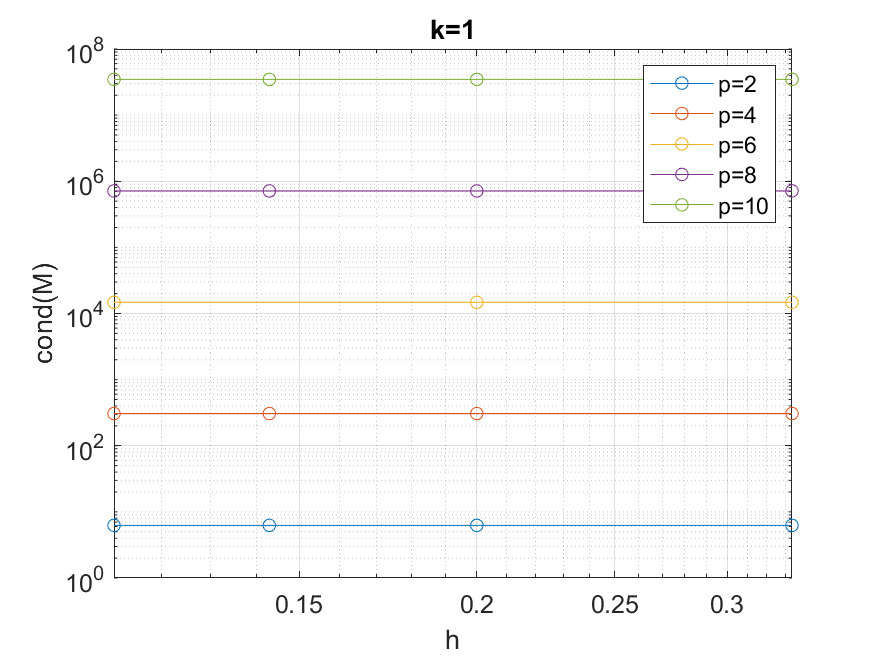
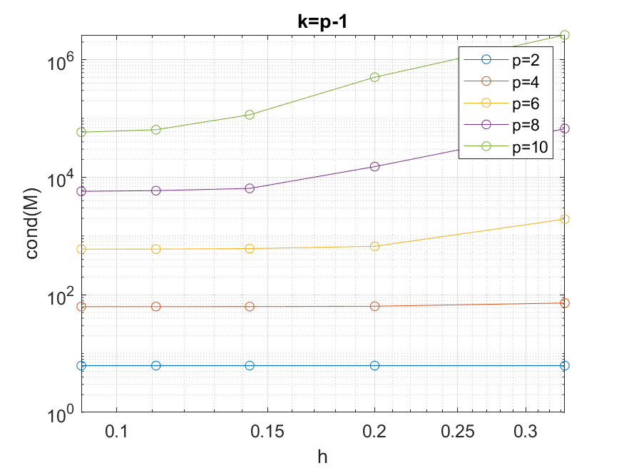
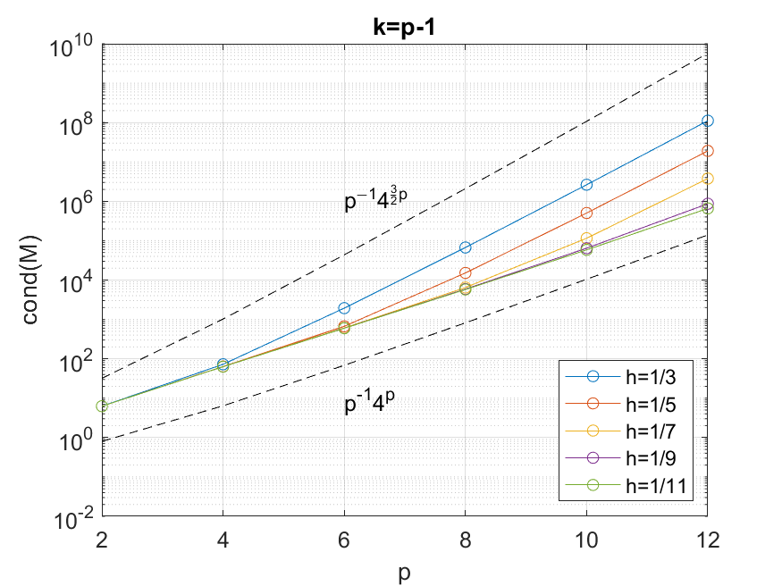
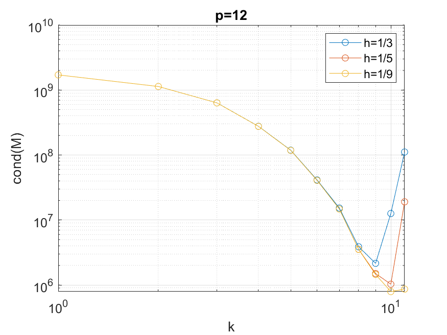
Figure 1: Condition number of the mass matrix versus: $h$ (top), for $p=2,4,6,8,10$, $k=1$ (left) or $k=p-1$ (right); $p$ (center), for $h=1/3,1/5,1/7,1/9$, $k=1$ (left) or $h=1/3,1/5,1/7,1/9,1/11$, $k=p-1$ (right); $k$ (bottom), for $h=1/3,1/5,1/9$, fixed $p=12$.

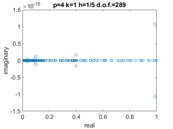
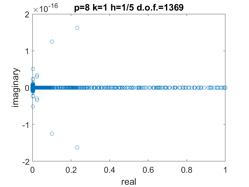
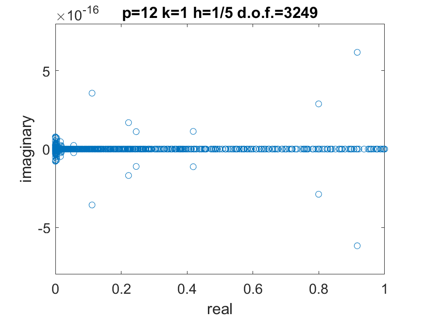
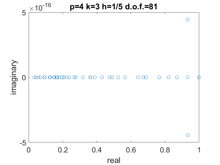
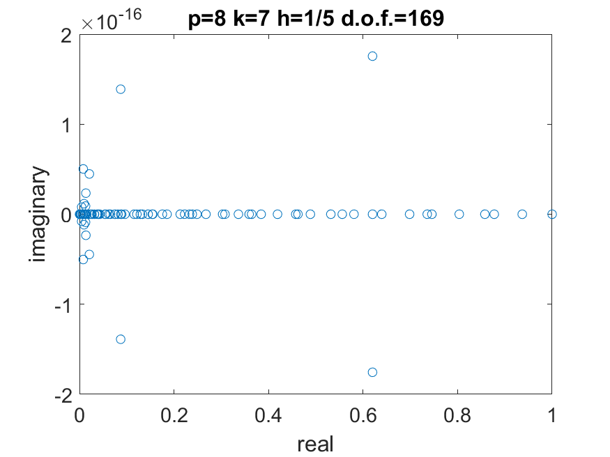
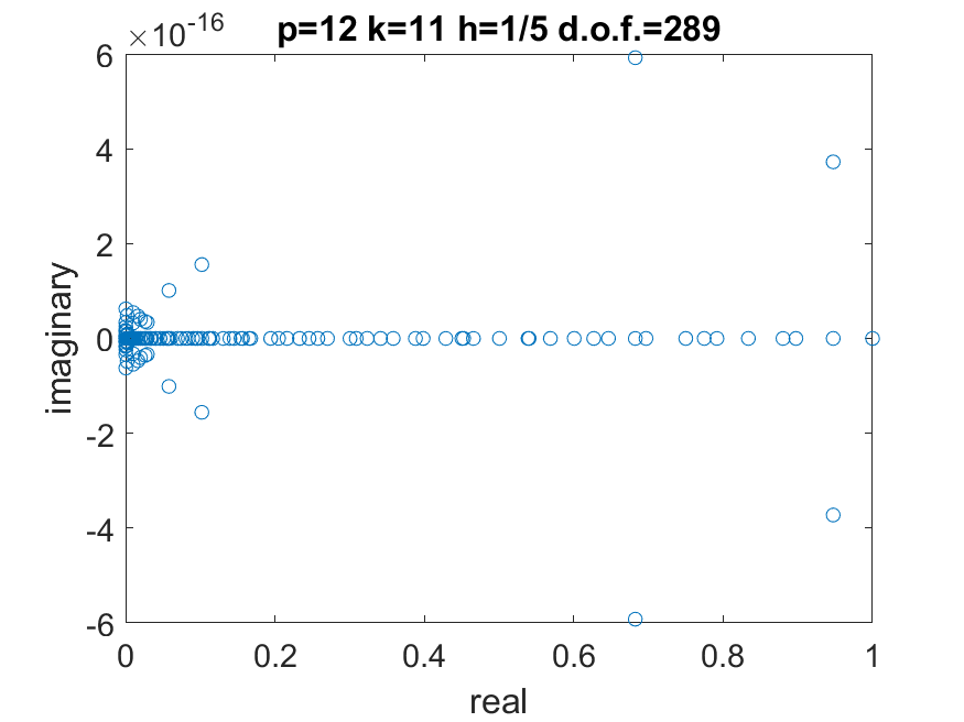
Figure 2: Mass matrix eigenvalue distribution in the complex plane, for $p=4$ (left), $p=8$ (center), $p=12$ (right), with $k=1$ (top) or $k=p-1$ (bottom), fixed $h=1/5$.

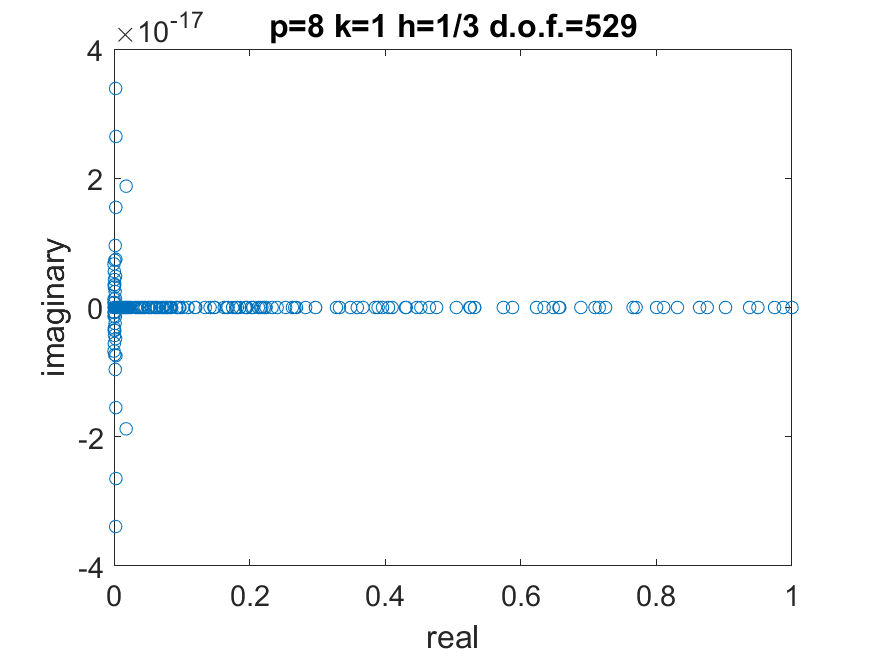
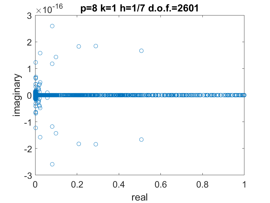
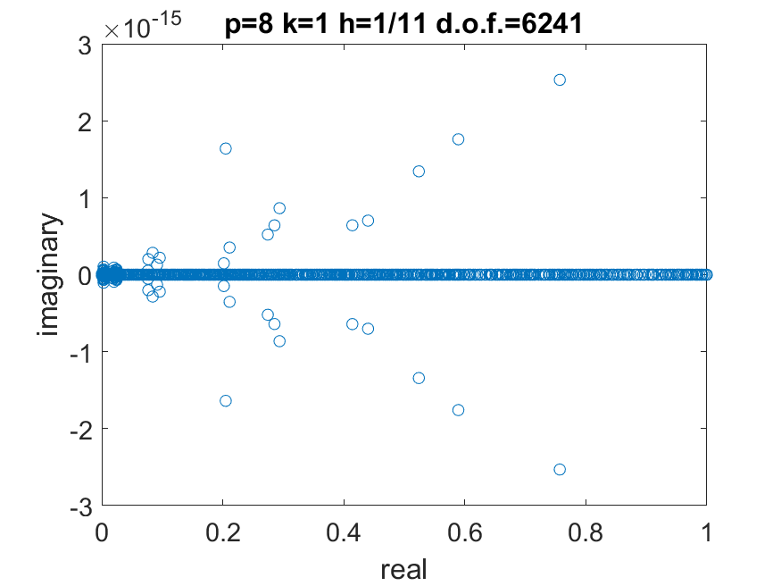
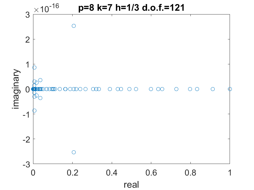
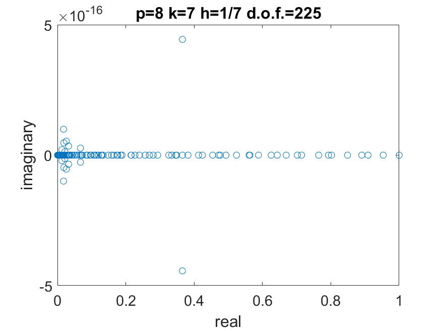
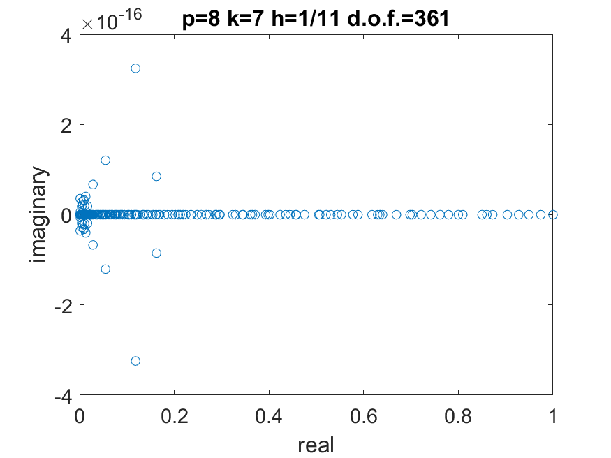
Figure 3: Mass matrix eigenvalue distribution in the complex plane, for $h=1/3$ (left), $1/h=7$ (center), $1/h=11$ (right), with $k=1$ (top) or $k=p-1$ (bottom), fixed $p=8$.

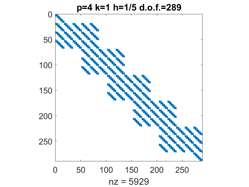
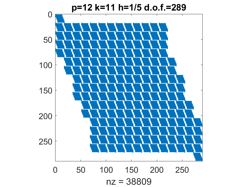
Figure 4: Mass matrix sparsity pattern, for $p=4$ (left), $p=8$ (center), $p=12$ (right), with $k=1$ (top) or $k=p-1$ (bottom), fixed $h=1/5$.

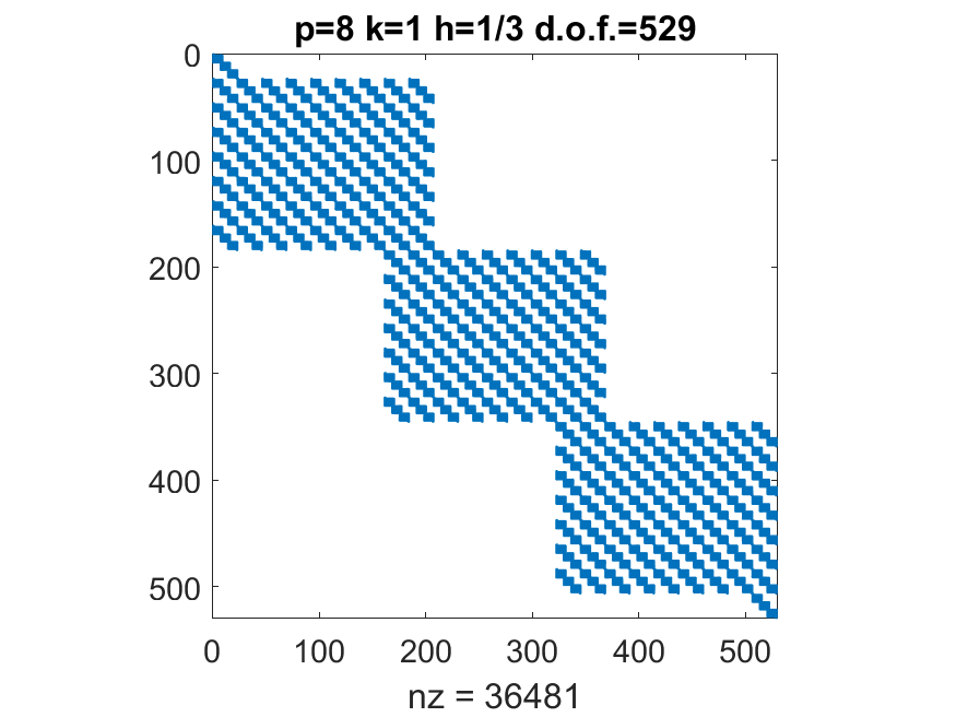
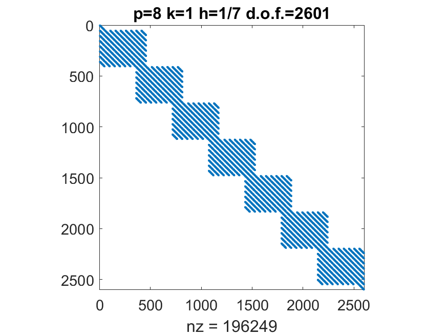
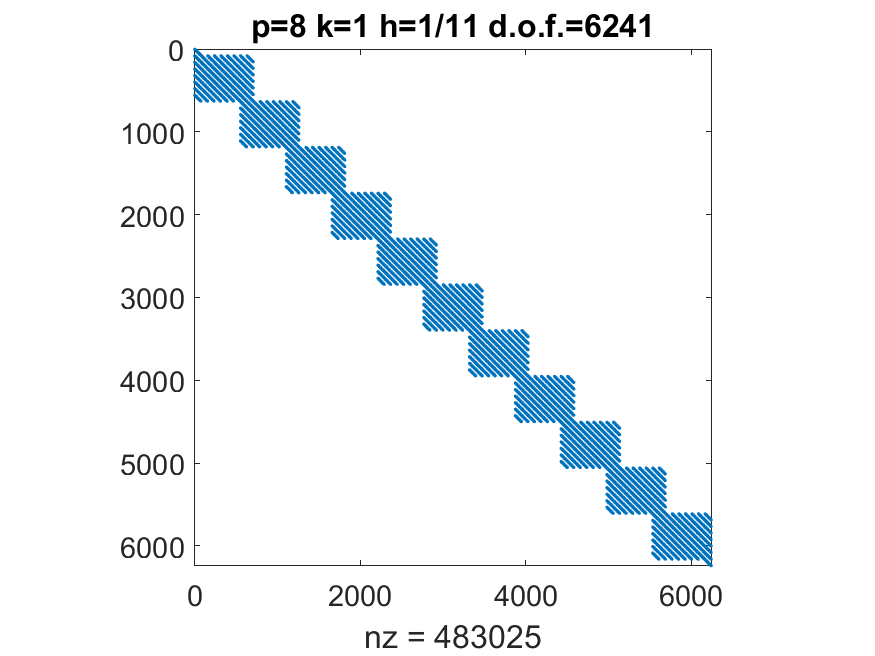
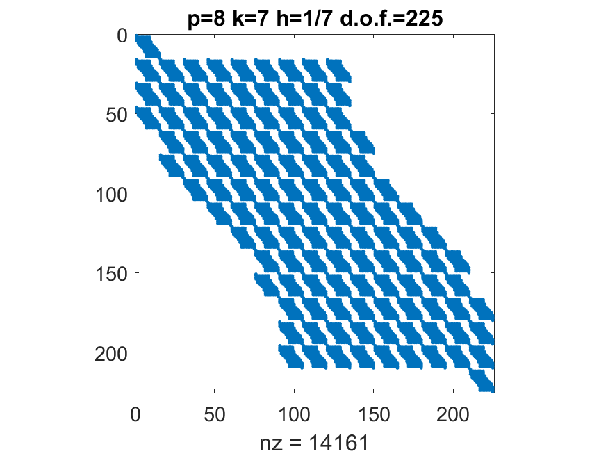
Figure 5: Mass matrix sparsity pattern, for $h=1/3$ (left), $1/h=7$ (center), $1/h=11$ (right), with $k=1$ (top) or $k=p-1$ (bottom), fixed $p=8$.

Eigenvalues and condition number of the stiffness matrix with Dirichlet and Neumann boundary conditions.

In Fig. 6, we report the condition numbers cond($\cal K$) of the stiffness matrix for the acoustic wave problem with Dirichlet boundary conditions, for $\Delta t=0.1$, $\beta=0$ (explicit Newmark scheme, left) or $\beta=0.5$ (implicit Newmark scheme, right), versus, from the top to the bottom: (1) the mesh size $h$, with five different values of degree $p$ and minimal regularity $k=1$, (2) the mesh size $h$, with five different values of degree $p$ and maximal regularity $k=p-1$, (3) the degree $p$, with four different values of mesh size $h$ and minimal regularity $k=1$, (4) the degree $p$, with five different values of mesh size $h$ and maximal regularity $k=p-1$. In Fig. 7, we consider the same tests as in Fig. 6 but with smaller time step $\Delta t=0.01$. The numerical results show that if $p$ is fixed, the condition numbers cond($\cal K$) are almost always independent of $h$ in both Figs. 6 and 7, except for the implicit scheme (right) in Fig. 6 where they seem to grow as $h^{-2}$, according to estimates (35)-(39). For the $p$- refinement with fixed $h$, it seems that the numerical results are better than these estimates. Indeed, the condition numbers cond($\cal K$) grow as $p^{-1}4^{\frac{3}{2}p}$ in the case of minimal regularity $k=1$, whereas for maximal regularity $k=p-1$ the growth ranges between $p^{-1}4^{p}$ and $p^{-1}4^{\frac{3}{2}p}$ for $\Delta t=0.1$, between $p^{-1}4^{\frac{1}{2}p}$ and $p^{-1}4^{p}$ in the implicit case with $\Delta t=0.01$, while the growth seems to be $p^{-1}4^{p}$ in the explicit case with $\Delta t=0.01$.

Figs. 8 and 9 reports the condition numbers cond($\cal K$) of the stiffness matrix for the acoustic wave problem with Neumann boundary conditions, using the same setting of Figs. 6 and 7, respectively. We note that if $p$ is fixed, the condition numbers cond($\cal K$) are almost always independent of $h$, in particular they do not increase when $h$ decreases, except in some cases with high $p$ for the explicit case with $\Delta t=0.1$, where the condition numbers scale at most as $h^{-2}$, as predicted by estimates (35)-(39). For the $p$- refinement, with fixed $h$, similarly to the Dirichlet case, the results are again better than the estimates (35)-(39). In fact, the condition numbers cond($\cal K$) scale as $p^{-1}4^{\frac{3}{2}p}$ in the case of minimal regularity $k=1$, whereas for maximal regularity $k=p-1$ they range between $p^{-1}4^{p}$ and $p^{-1}4^{\frac{3}{2}p}$ for $\Delta t=0.1$, range between $p^{-1}4^{\frac{1}{2}p}$ and $p^{-1}4^{p}$ in the explicit case with $\Delta t=0.01$, and scale as $p^{-1}4^{p}$ in the implicit case with $\Delta t=0.01$.

Fig. 10 reports the stiffness matrix $\cal K$ eigenvalue distribution in the complex plane for the acoustic wave problem with Dirichlet boundary conditions, for $\Delta t=0.01$, $\gamma=0.5$, $\beta=0.5$. We consider three different values of degree $p=4$ (left), $p=8$ (center), $p=12$ (right), minimal regularity $k=1$ (top) or maximal regularity $k=p-1$ (bottom), for fixed $h=1/5$. In Fig. 11, we use the same setting to report the analogous eigenvalue distributions for three different values of mesh size $h=1/3$ (left), $h=1/7$ (center), $h=1/11$ (right), minimal regularity $k=1$ (top) or maximal regularity $k=p-1$ (bottom), for fixed $p=8$. The eigenvalues real parts belong to an interval $[0,r]$ where $r$ increases with both $1/h$ and $p$, but for fixed $p$ and $h$, $r$ is approximately the same for both minimal regularity $k=1$ and maximal regularity $k=p-1$. On the other hand, the eigenvalue imaginary parts are negligible for maximal regularity $k=p-1$, while for minimal regularity $k=1$ the eigenvalues imaginary parts belong to an interval $[-s,s]$ where $s$ increases with both $1/h$ and $p$.

Figs. 12 and 13 shows the sparsity pattern of the stiffness matrix $\cal K$ for the same problem and parameter settings as in Figs. 10 and 11, respectively. The results are analogous to those for the mass matrices in Figs. 4 and 5, with block-diagonal matrices for minimal regularity and almost full matrices in the case of maximal regularity. Again, both d.o.f. and nz decrease for increasing regularity.

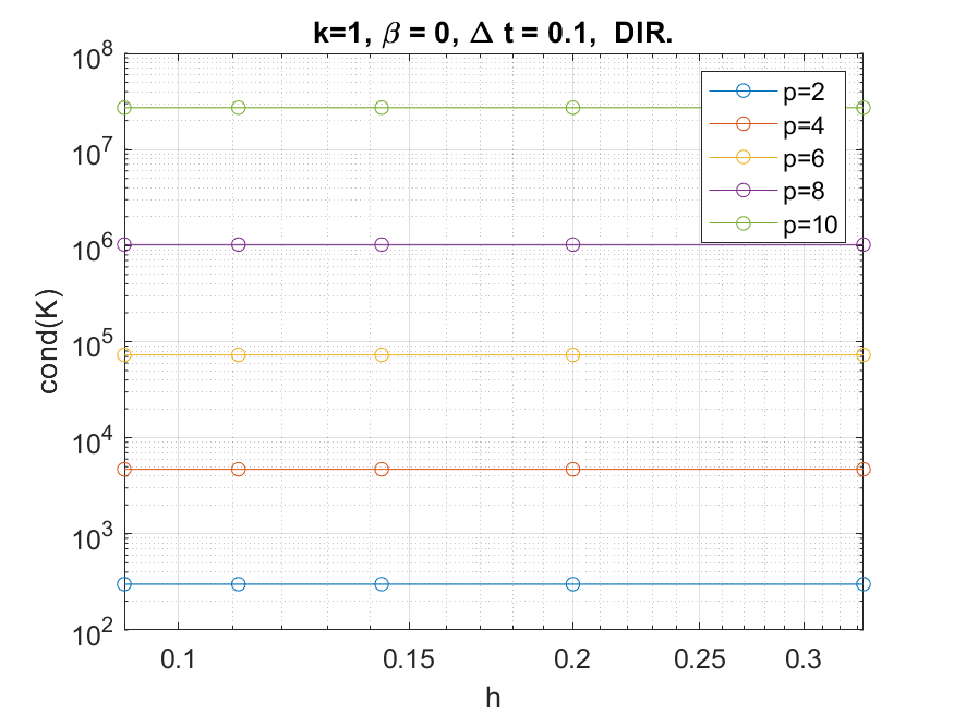
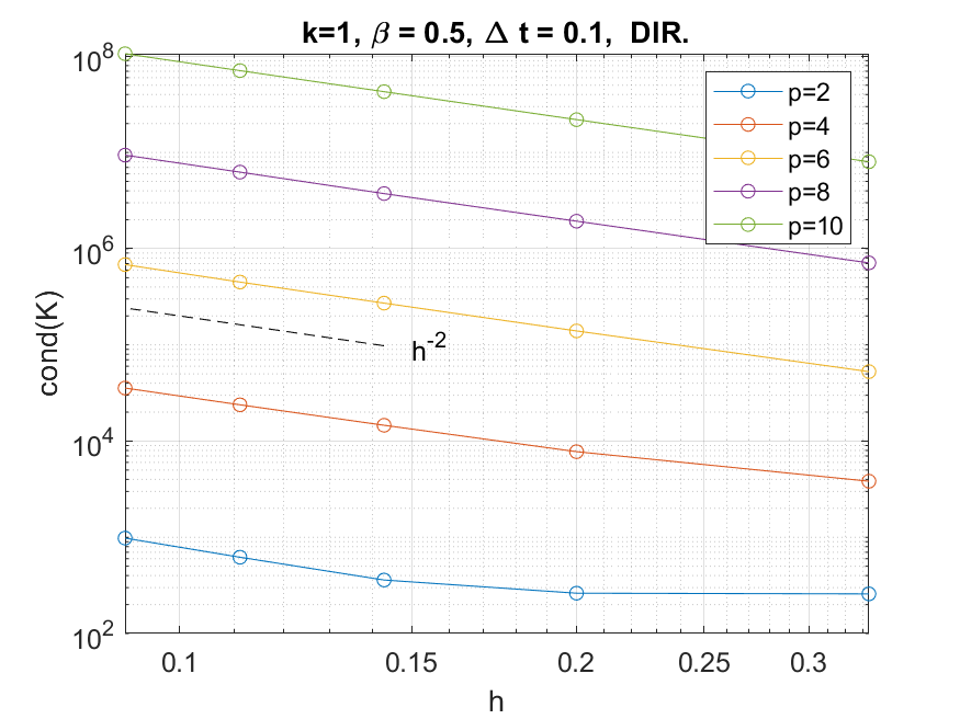
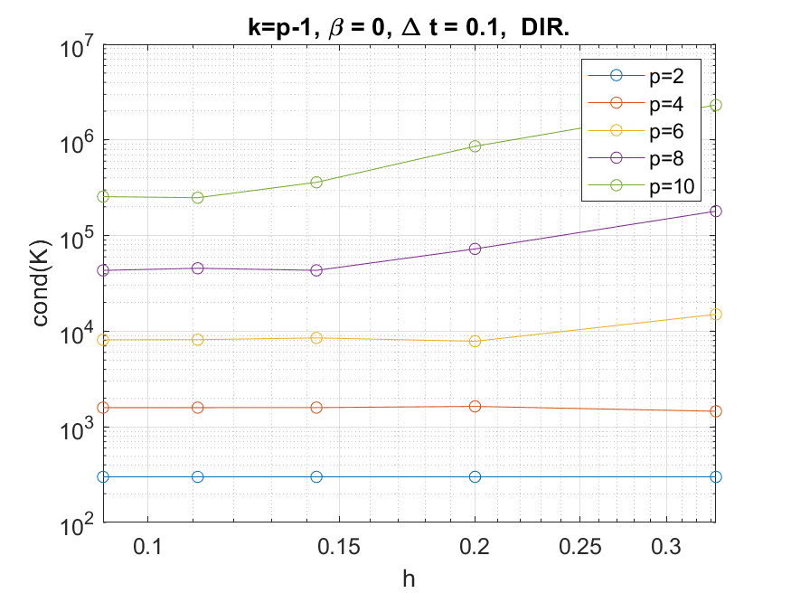
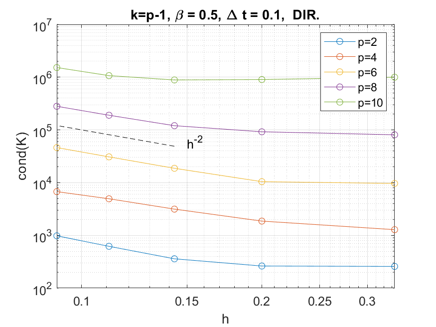
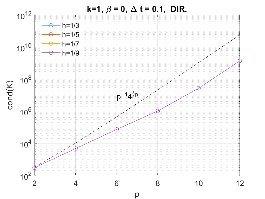
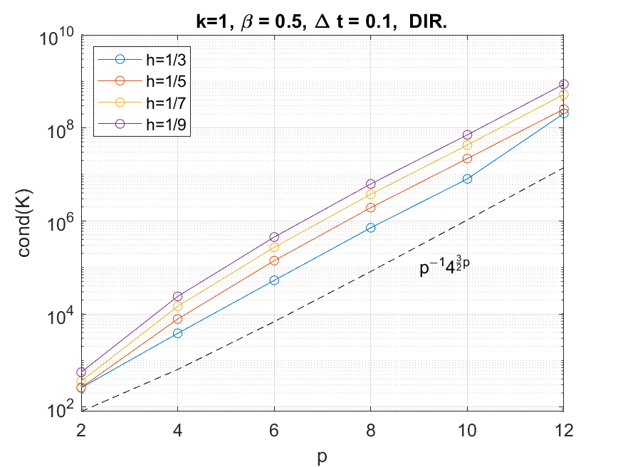
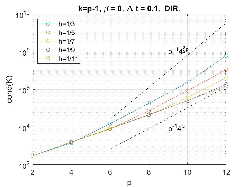
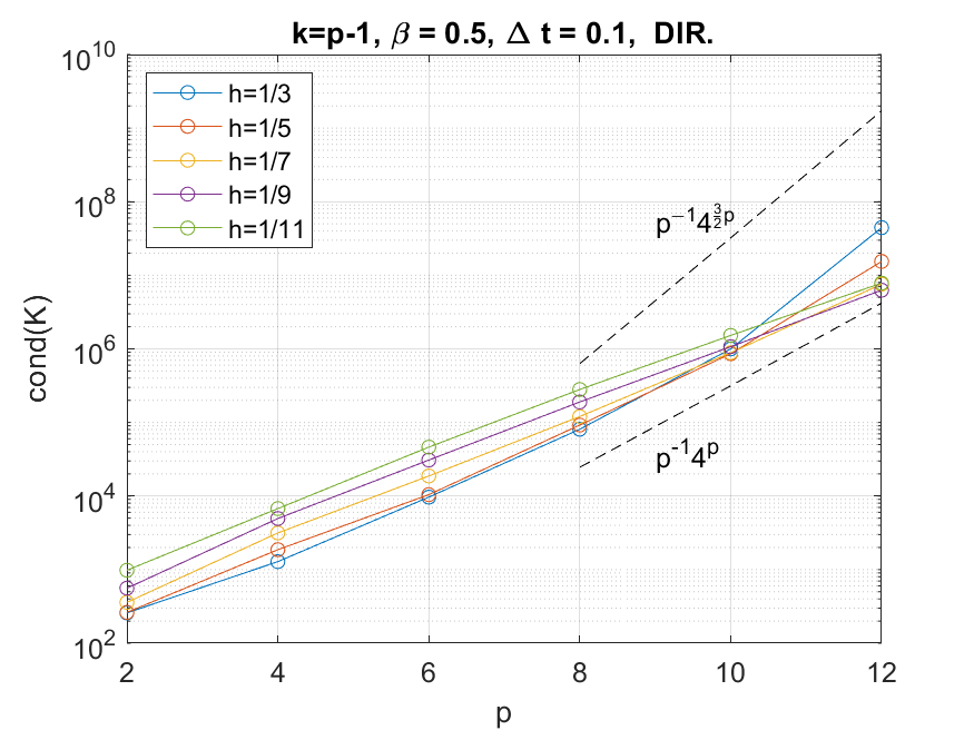
Figure 6: Condition number of the stiffness matrix for the acoustic wave problem with Dirichlet boundary conditions, $\Delta t=0.1$, $\gamma=0.5$, $\beta=0$ (explicit Newmark, left), $\beta=0.5$ (implicit Newmark, right). From the top to the bottom, vs.: (1) $h$, for $p=2,4,6,8,10$, $k=1$; (2) $h$, for $p=2,4,6,8,10$, $k=p-1$; (3) $p$, for $h=1/3,1/5,1/7,1/9$, $k=1$; (4) $p$, for $h=1/3,1/5,1/7,1/9,1/11$, $k=p-1$.

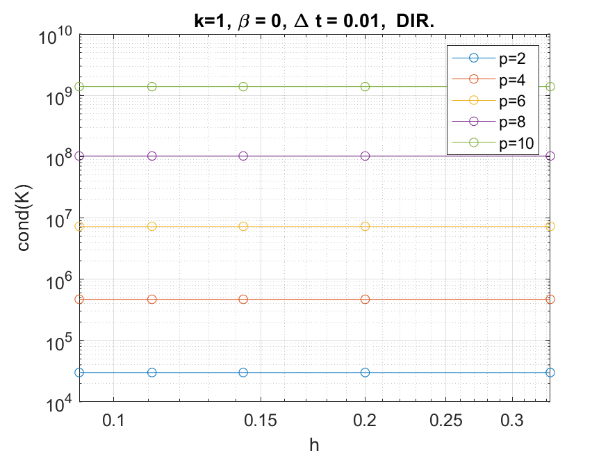
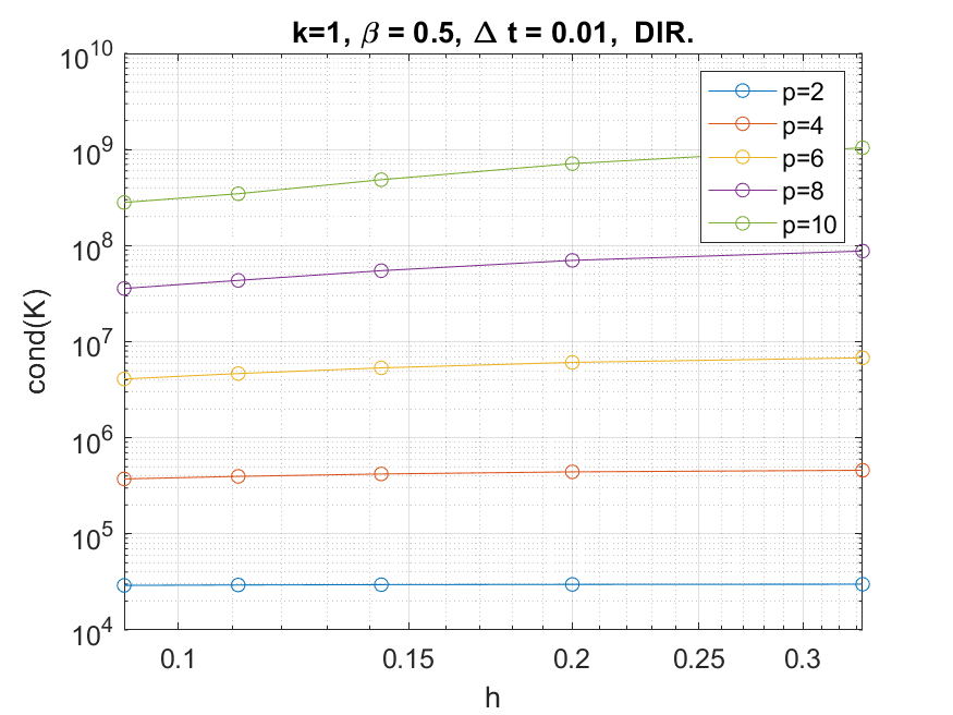
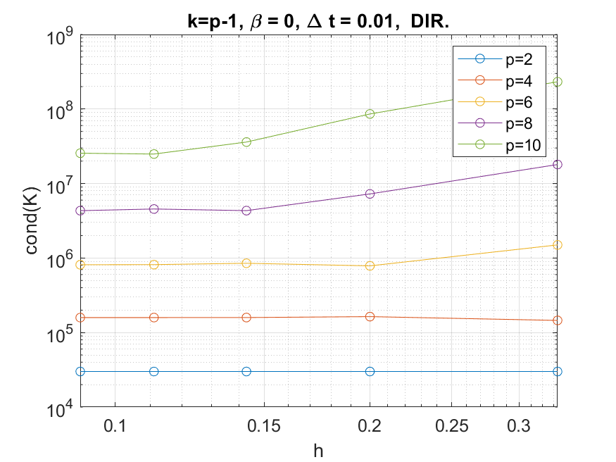
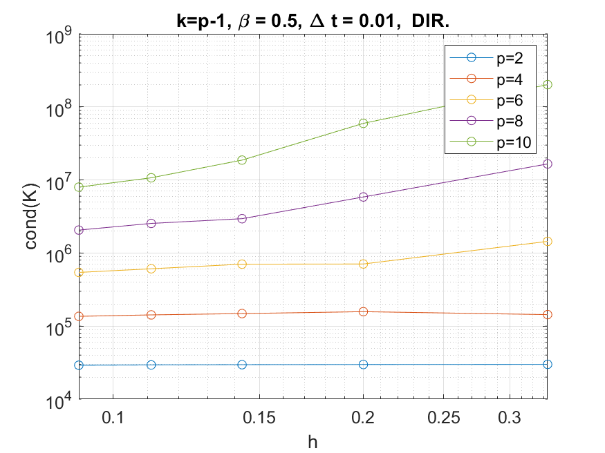
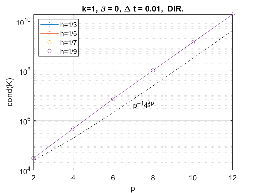
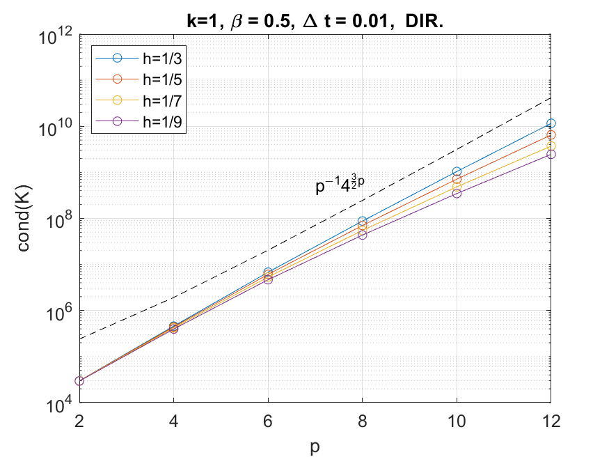
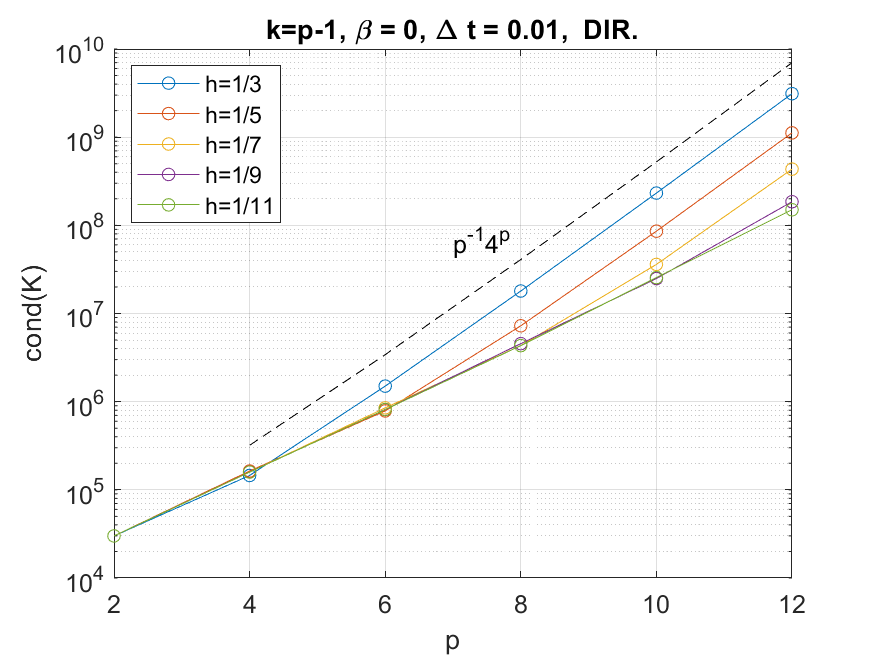
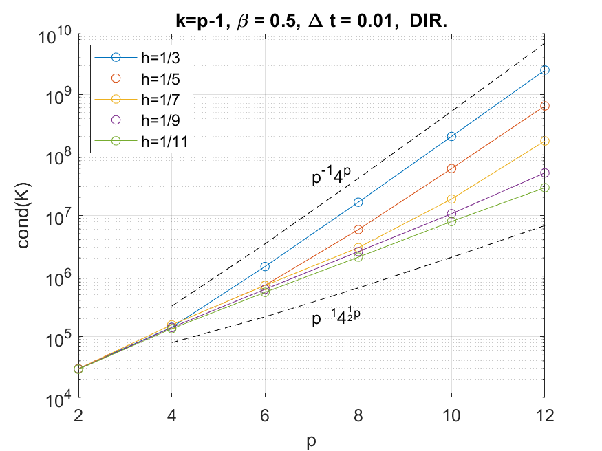
Figure 7: Condition number of the stiffness matrix for the acoustic wave problem with Dirichlet boundary conditions, $\Delta t=0.01$, $\gamma=0.5$, $\beta=0$ (explicit Newmark, left), $\beta=0.5$ (implicit Newmark, right). From the top to the bottom, vs.: (1) $h$, for $p=2,4,6,8,10$, $k=1$; (2) $h$, for $p=2,4,6,8,10$, $k=p-1$; (3) $p$, for $h=1/3,1/5,1/7,1/9$, $k=1$; (4) $p$, for $h=1/3,1/5,1/7,1/9,1/11$, $k=p-1$.

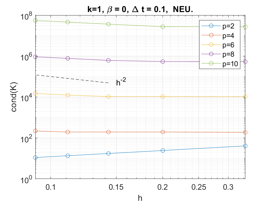
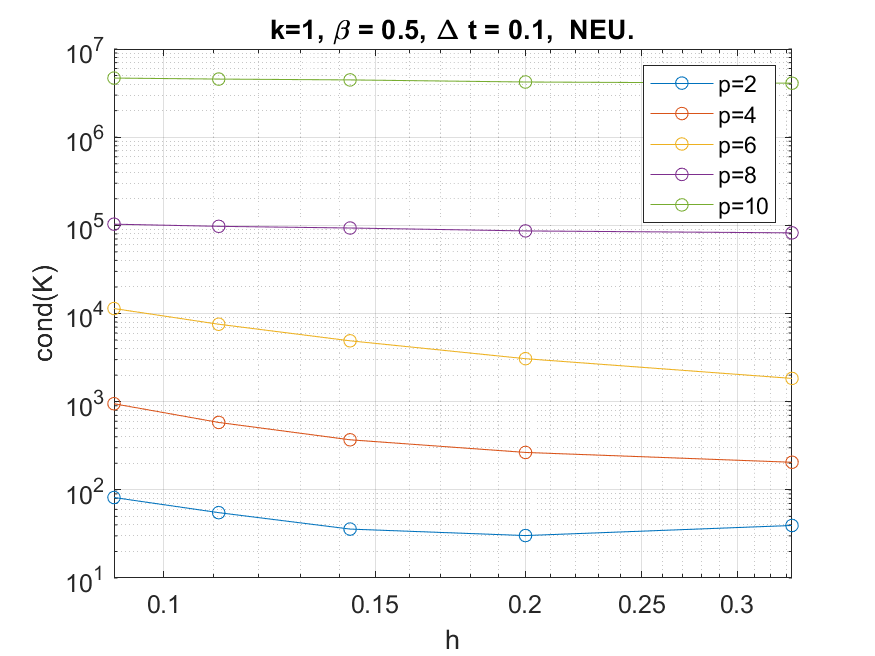
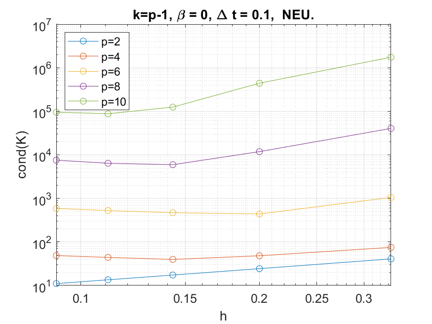
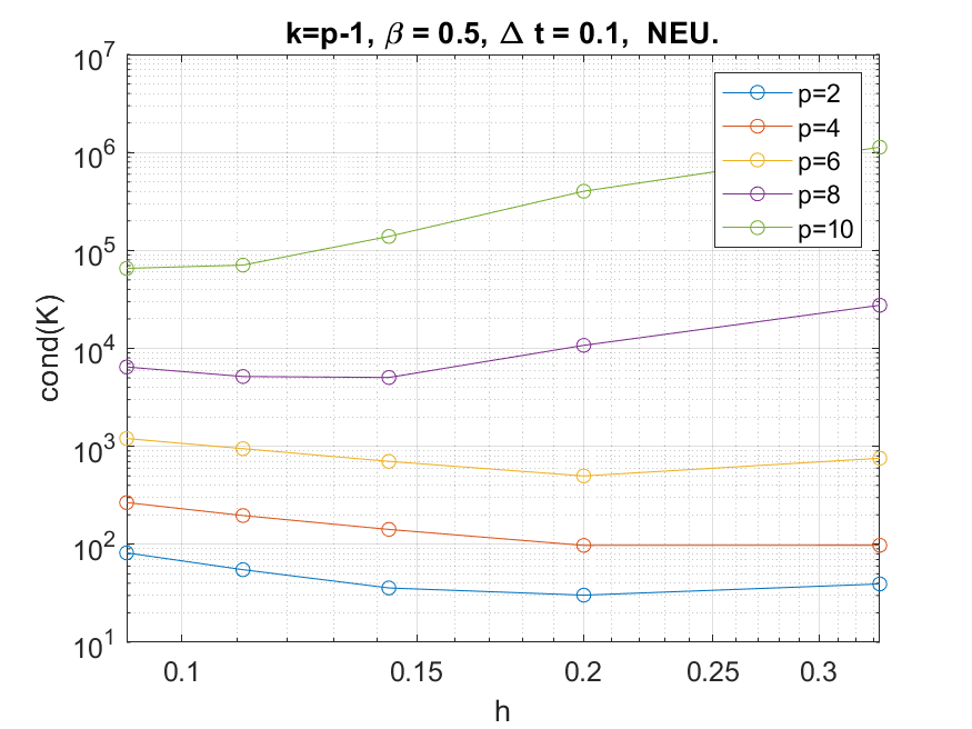
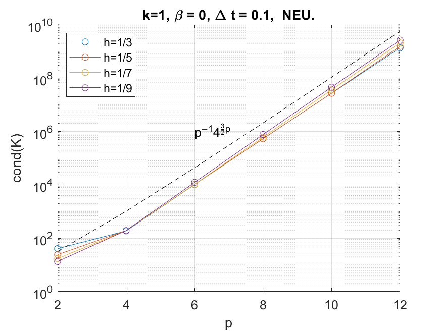
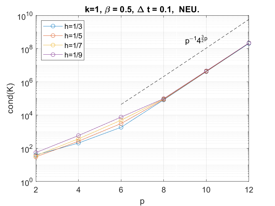
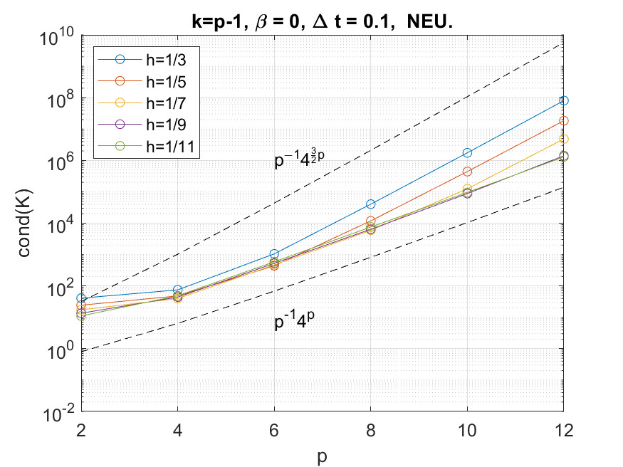
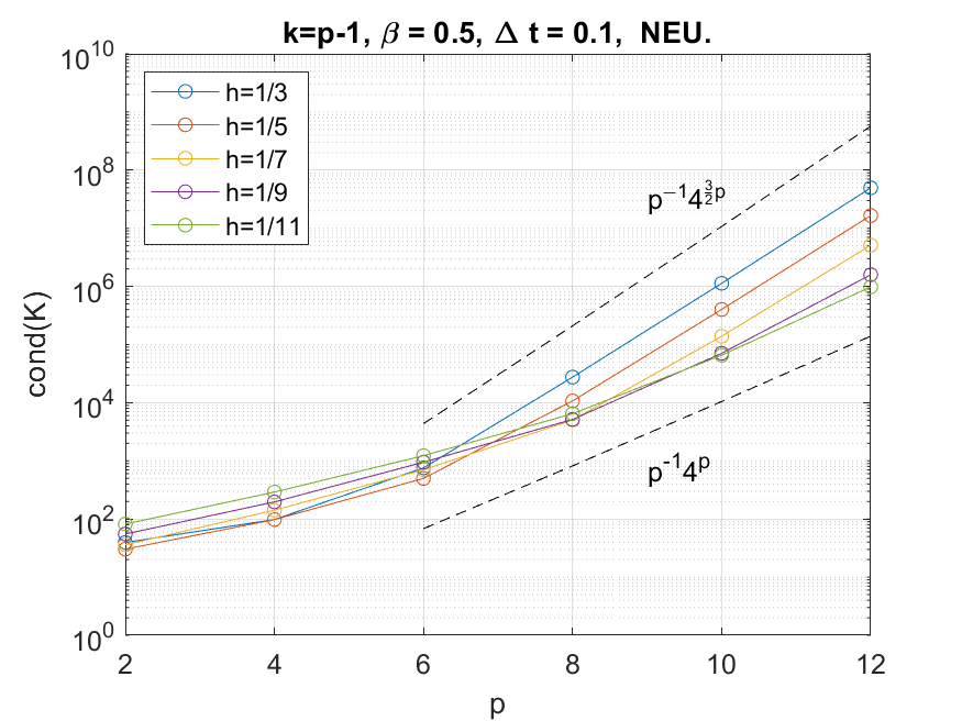
Figure 8: Condition number of the stiffness matrix for the acoustic wave problem with Neumann boundary conditions, $\Delta t=0.1$, $\gamma=0.5$, $\beta=0$ (explicit Newmark, left), $\beta=0.5$ (implicit Newmark, right). From the top to the bottom, vs.: (1) $h$, for $p=2,4,6,8,10$, $k=1$; (2) $h$, for $p=2,4,6,8,10$, $k=p-1$; (3) $p$, for $h=1/3,1/5,1/7,1/9$, $k=1$; (4) $p$, for $h=1/3,1/5,1/7,1/9,1/11$, $k=p-1$.

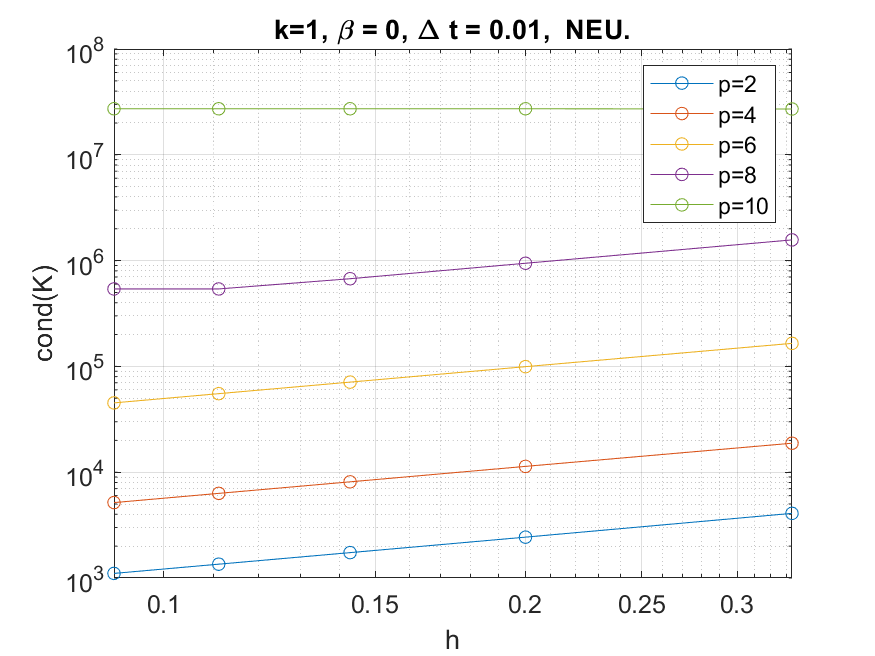
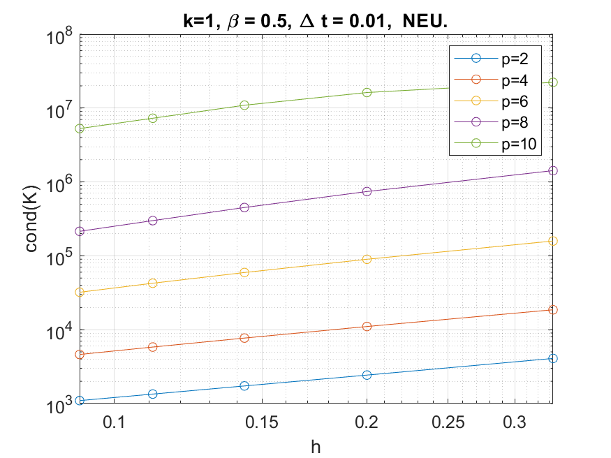
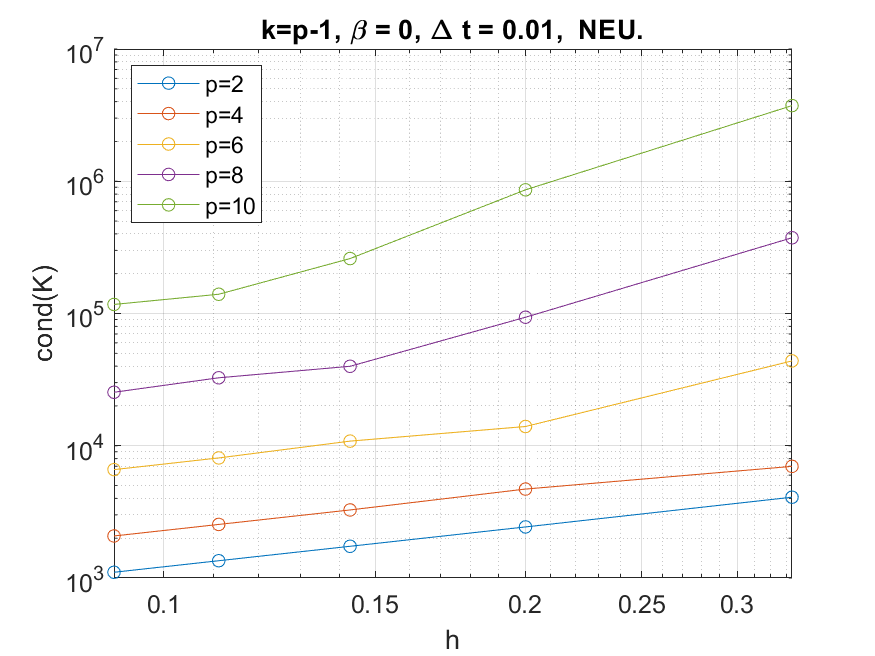
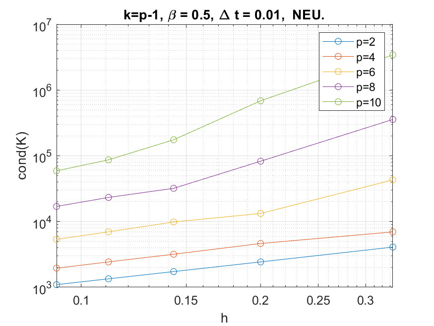
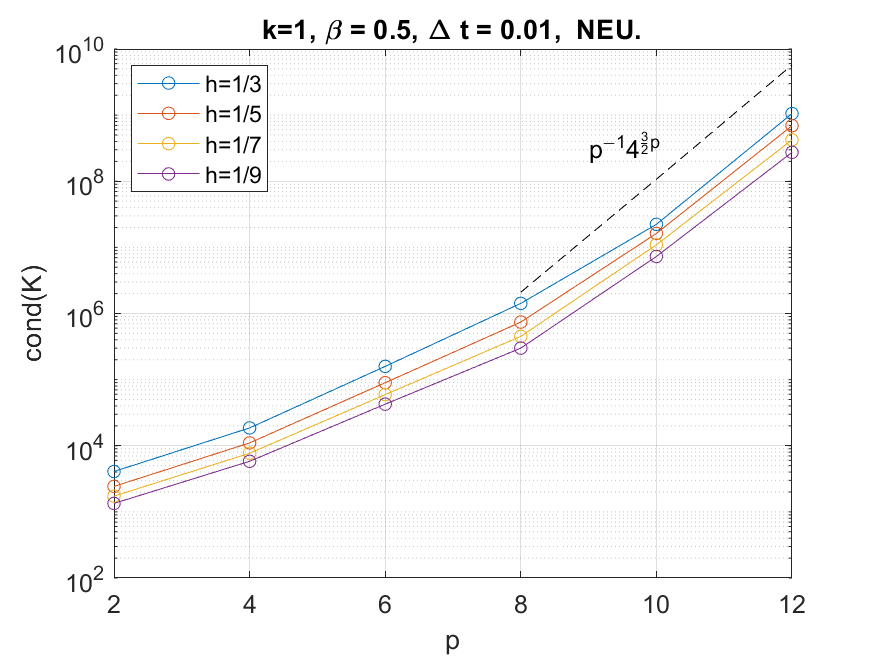
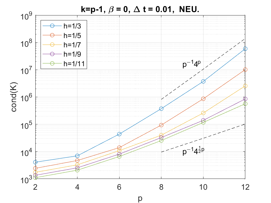
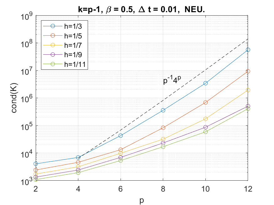
Figure 9: Condition number of the stiffness matrix for the acoustic wave problem with Neumann boundary conditions, $\Delta t=0.01$, $\gamma=0.5$, $\beta=0$ (explicit Newmark, left), $\beta=0.5$ (implicit Newmark, right). From the top to the bottom, vs.: (1) $h$, for $p=2,4,6,8,10$, $k=1$; (2) $h$, for $p=2,4,6,8,10$, $k=p-1$; (3) $p$, for $h=1/3,1/5,1/7,1/9$, $k=1$; (4) $p$, for $h=1/3,1/5,1/7,1/9,1/11$, $k=p-1$.

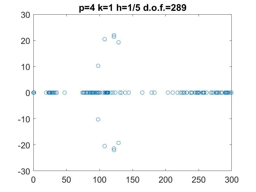
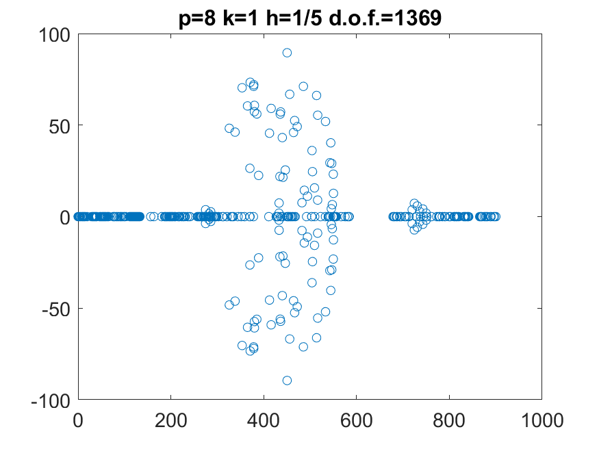
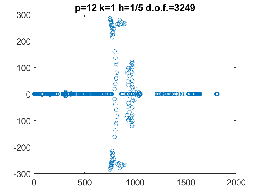
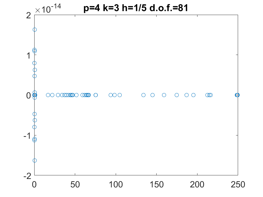
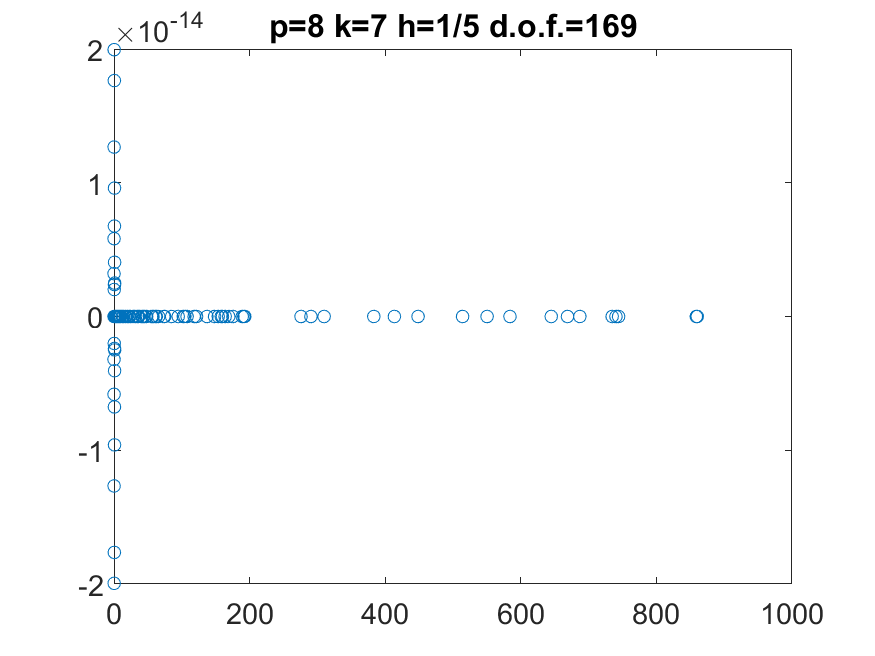
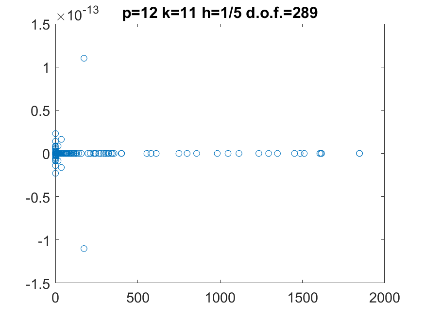
Figure 10: Stiffness matrix eigenvalue distribution in the complex plane for the acoustic wave problem with Dirichlet boundary conditions: $p=4$ (left), $p=8$ (center), $p=12$ (right), with $k=1$ (top) or $k=p-1$ (bottom), fixed $h=1/5$, $\Delta t=0.01$, $\gamma=0.5$, $\beta=0.5$.

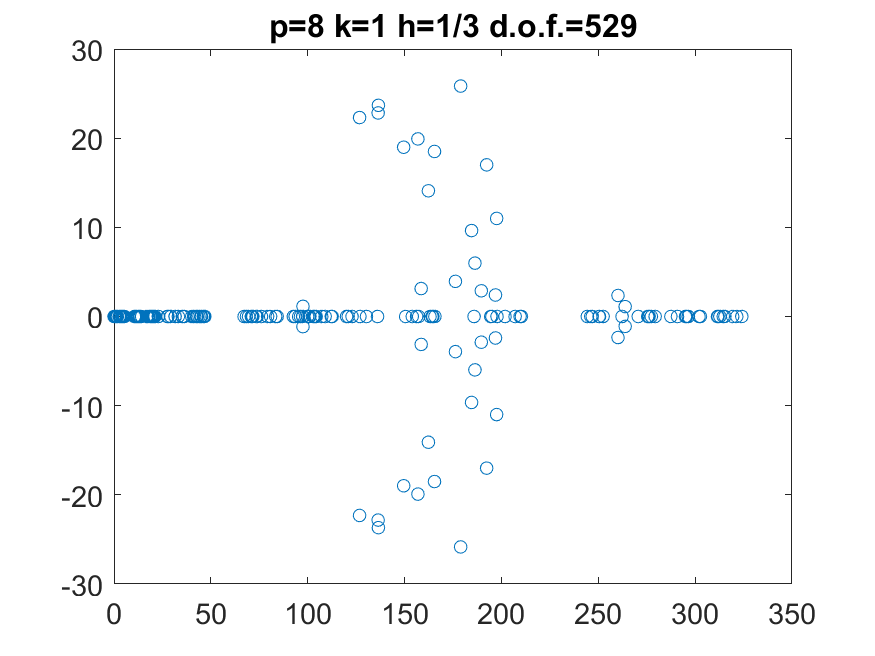
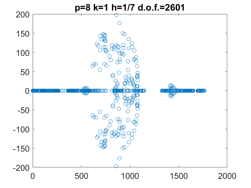
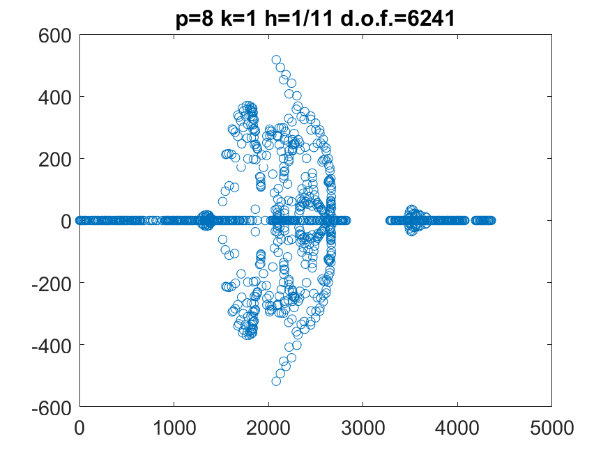
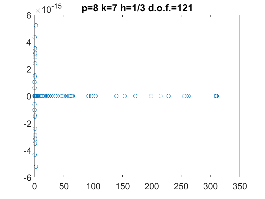
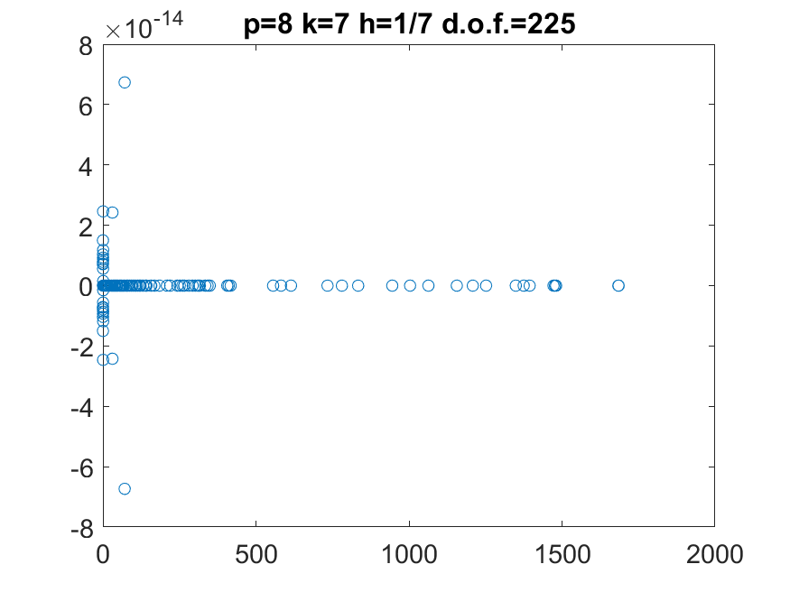
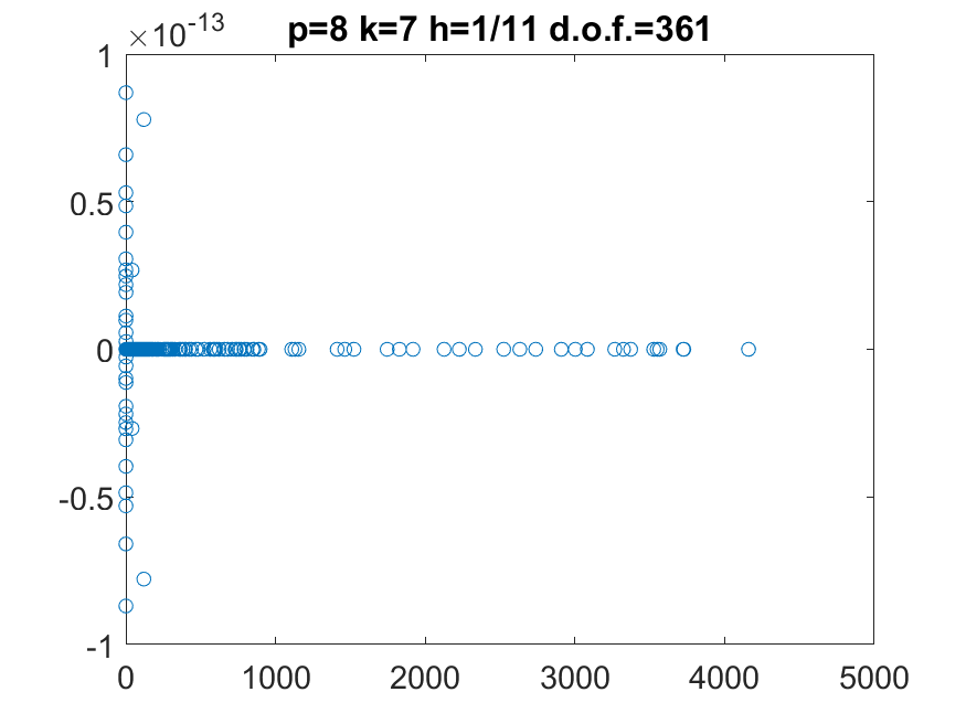
Figure 11: Stiffness matrix eigenvalue distribution in the complex plane for the acoustic wave problem with Dirichlet boundary conditions: $h=1/3$ (left), $1/h=7$ (center), $1/h=11$ (right), with $k=1$ (top) or $k=p-1$ (bottom), fixed $p=8$, $\Delta t=0.01$, $\gamma=0.5$, $\beta=0.5$.

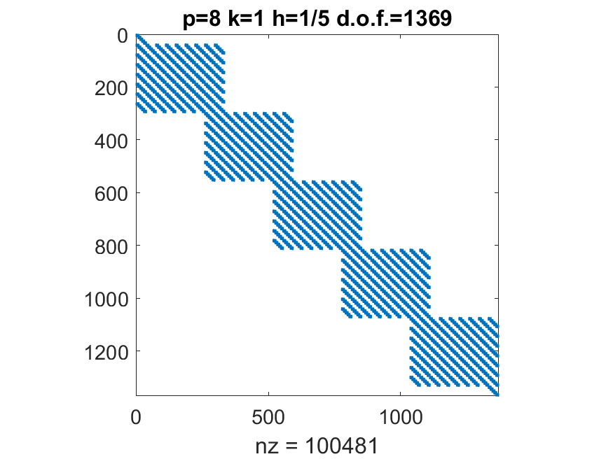
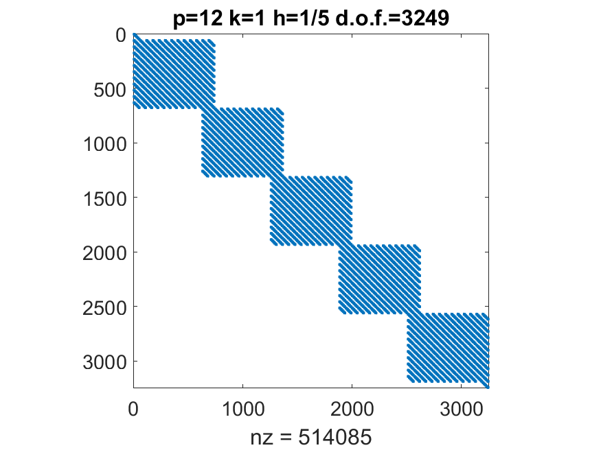
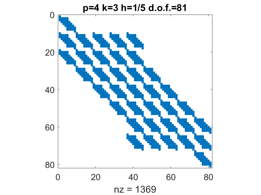
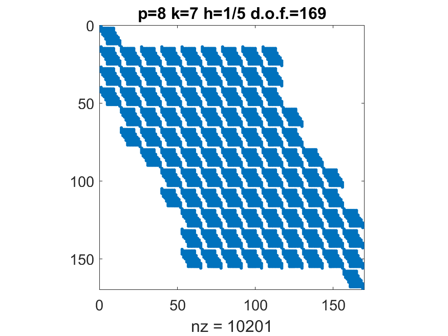
Figure 12: Stiffness matrix sparsity pattern for the acoustic wave problem with Dirichlet boundary conditions: $p=4$ (left), $p=8$ (center), $p=12$ (right), with $k=1$ (top) or $k=p-1$ (bottom), fixed $h=1/5$, $\Delta t=0.01$, $\gamma=0.5$, $\beta=0.5$.

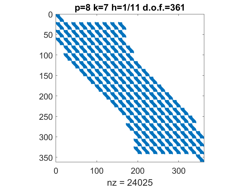
Figure 13: Stiffness matrix sparsity pattern for the acoustic wave problem with Dirichlet boundary conditions: for $h=1/3$ (left), $1/h=7$ (center), $1/h=11$ (right), with $k=1$ (top) or $k=p-1$ (bottom), fixed $p=8$, $\Delta t=0.01$, $\gamma=0.5$, $\beta=0.5$.

Eigenvalues and condition number of the stiffness matrix with absorbing boundary conditions.

In Fig. 14 and 15 we report the condition numbers cond($\cal K$) of the stiffness matrix for the acoustic wave problem with absorbing boundary conditions (4), using the same setting of Figs. 6 and 7, respectively. We observe that the results are analogous to those for Neumann conditions.

In Fig. 16 we report the condition numbers cond($\cal K$) of the stiffness matrix for the acoustic wave problem with different types of boundary conditions: absorbing (top), Dirichlet (center), Neumann (bottom). We vary the values of regularity $k$, and choose $\beta=0$ (explicit Newmark), $\gamma=0.5$, degree $p=12$, $\Delta t=0.1$ (left) or $\Delta t=0.01$ (right), and three different values of mesh size $h$. The results are analogous to those for the mass matrices in Fig. 1 for each type of boundary conditions.

In Fig. 17 and 18 we report the stiffness matrix $\cal K$ eigenvalue distribution in complex plane for the acoustic wave problem with absorbing boundary conditions, and explicit Newmark scheme ($\beta=0)$, for $\Delta t=0.01$ and $\gamma=0.5$. Results refer to the same parameter settings as in Figs. 10 and 11. The eigenvalues real parts belong to an interval $[0,r]$ with $r$ independent of all parameters $1/h$, $p$ and $k$. Here the value $r$ is much larger than in the case of Dirichlet boundary conditions. Furthermore, the real parts of complex eigenvalues are almost close to zero.

Figs. 19 and 20 report the sparsity pattern of the stiffness matrix $\cal K$ for the the acoustic wave problem with absorbing boundary conditions, explicit Newmark scheme ($\beta=0)$, for the same parameter settings as in Figs. 10 and 11, respectively. The results are similar, with block-diagonal matrices for minimal regularity and almost full matrices in the case of maximal regularity. Again, both d.o.f. and nz decrease for increasing regularity. In Figs. 21, 22, 23, and 24, we report the same data as in Figs. 17, 18, 19, and 20, respectively, for implicit Newmark scheme ($\beta=0.5)$, all other values of parameters being unchanged. The sparsity pattern are similar to the explicit case, but we observe definitely fewer complex eigenvalues.

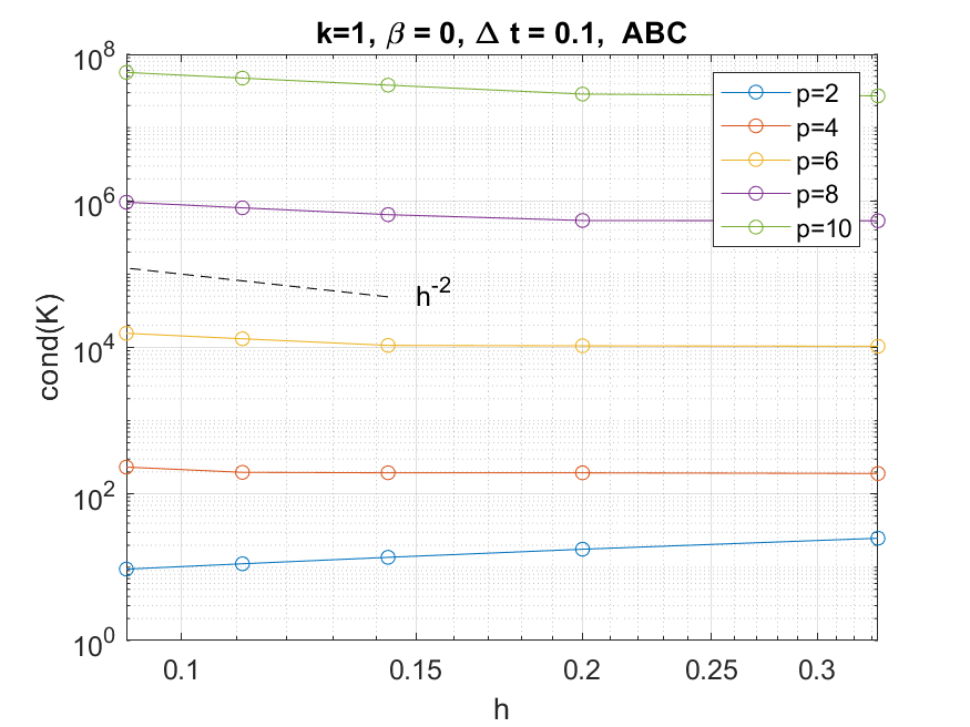
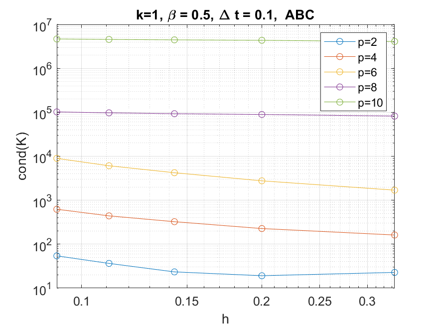
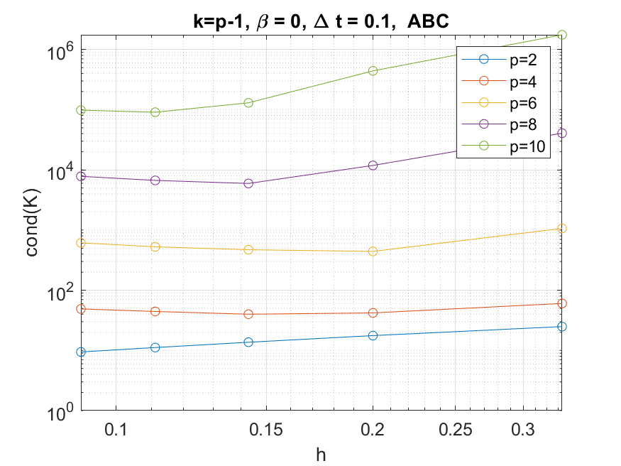
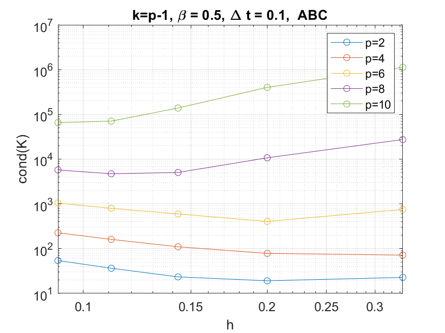
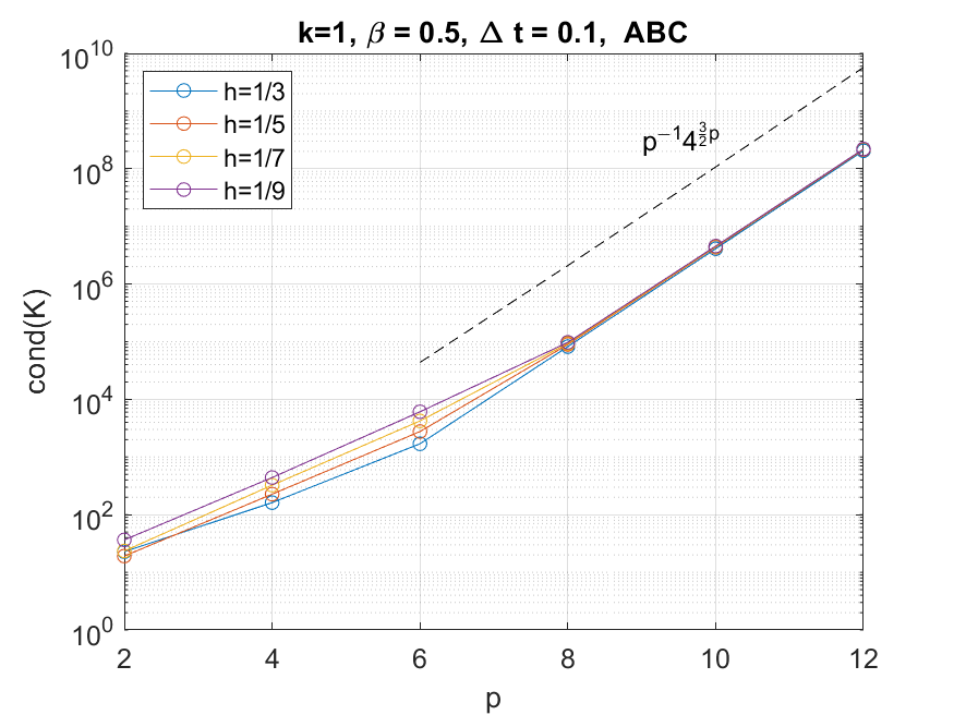
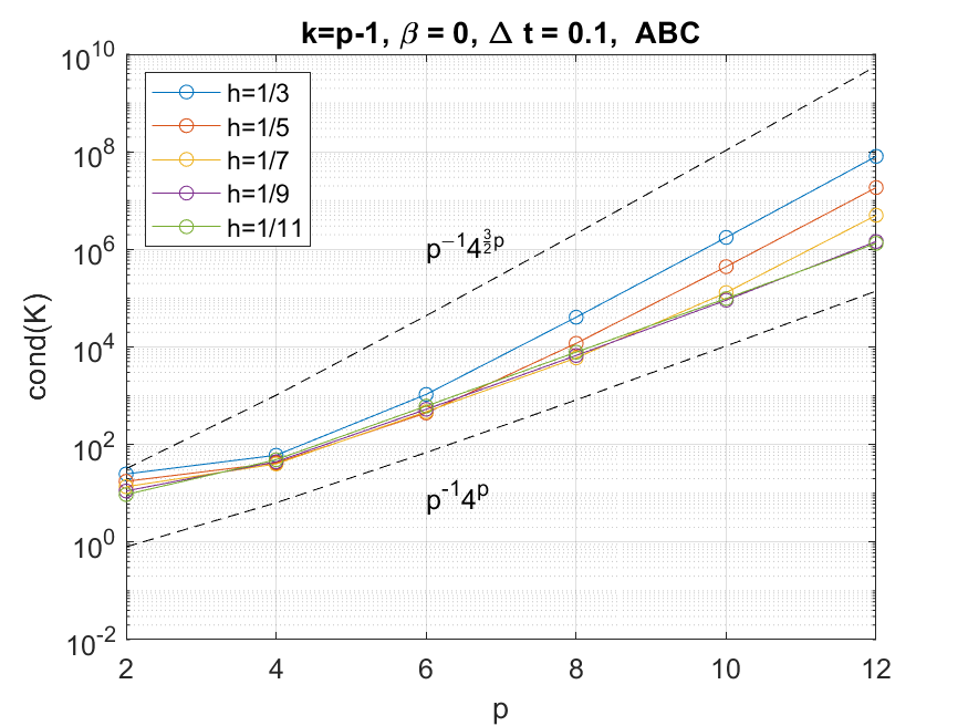
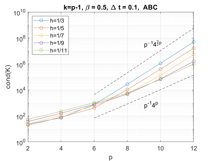
Figure 14: Condition number of the stiffness matrix for the acoustic wave problem with absorbing boundary conditions (4), $\Delta t=0.1$, $\gamma=0.5$, $\beta=0$ (explicit Newmark, left), $\beta=0.5$ (implicit Newmark, right). From the top to the bottom, vs.: (1) $h$, for $p=2,\ 4,\ 6,8,\ 10$, $k=1$; (2) $h$, for $p=2,\ 4,\ 6,8,\ 10$, $k=p-1$; (3) $p$, for $h=1/3,\ 1/5,\ 1/7,\ 1/9$, $k=1$; (4) $p$, for $h=1/3,\ 1/5,\ 1/7,\ 1/9,\ 1/11$, $k=p-1$.

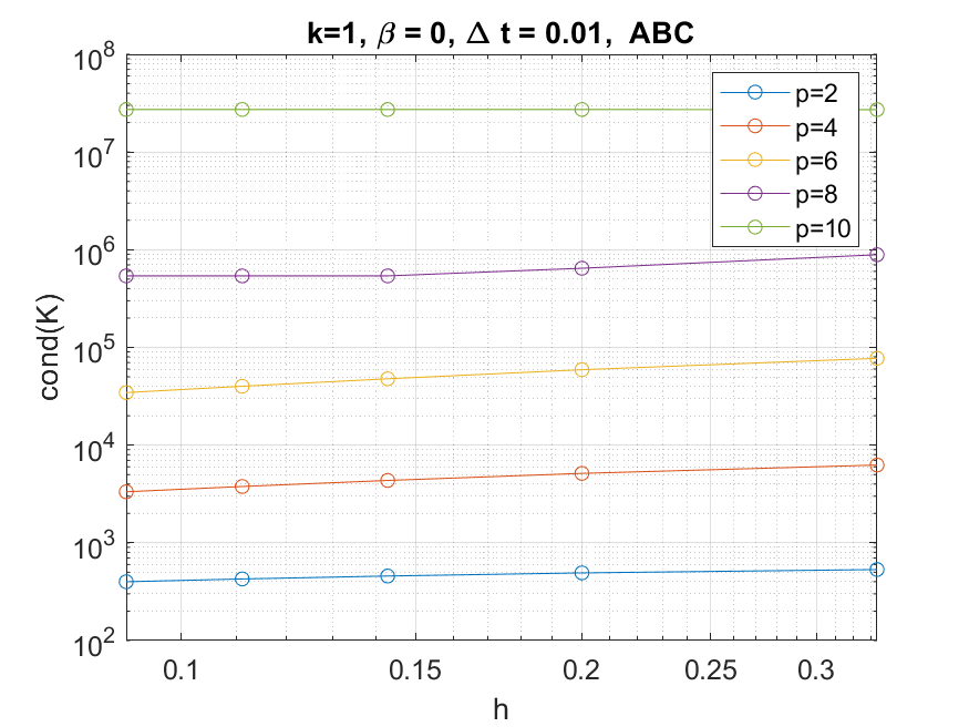
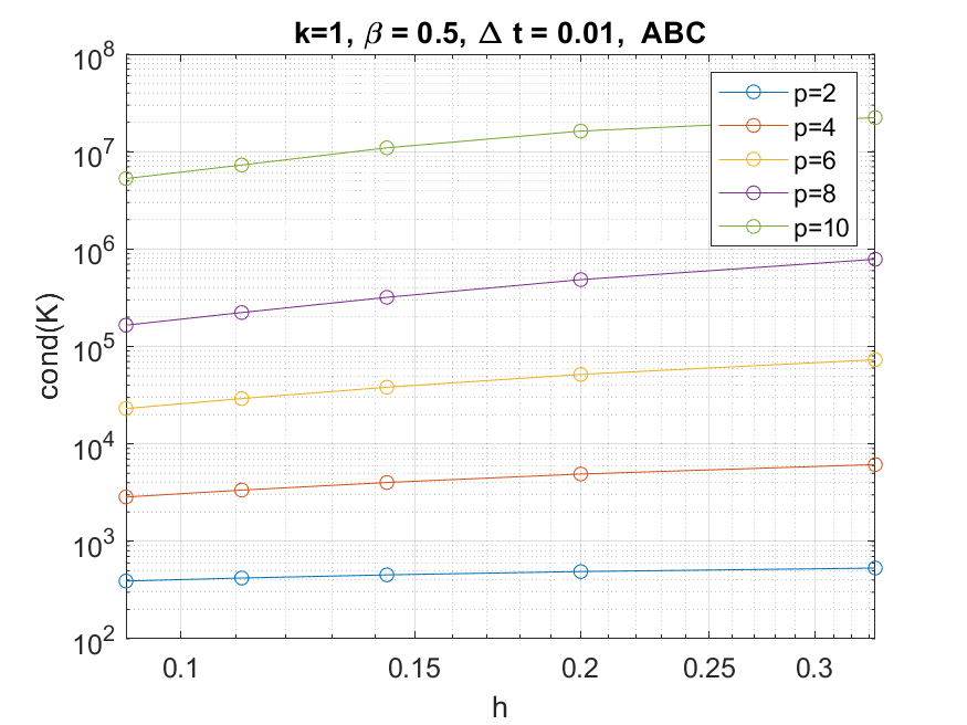
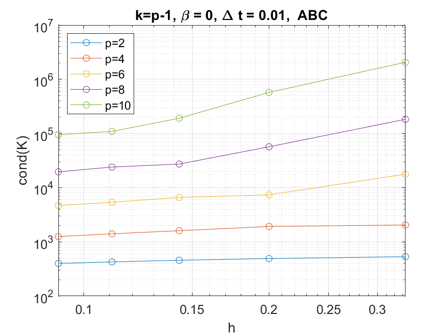
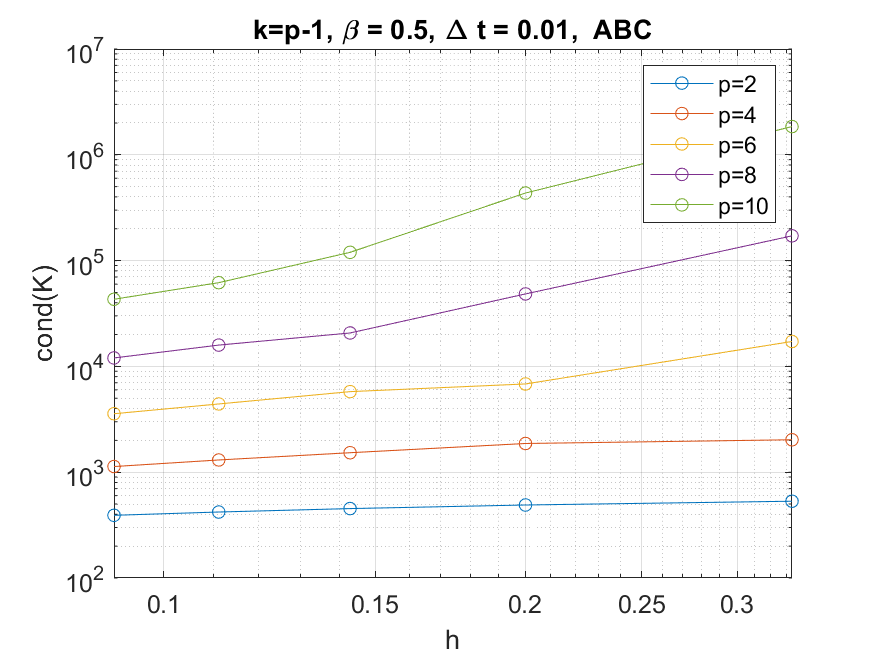
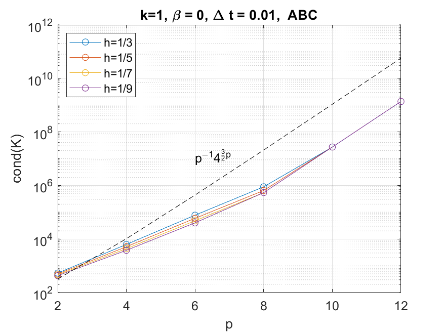
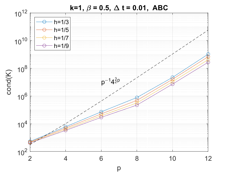
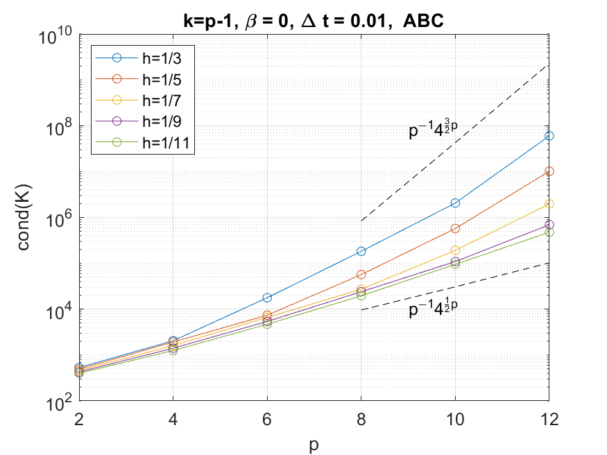
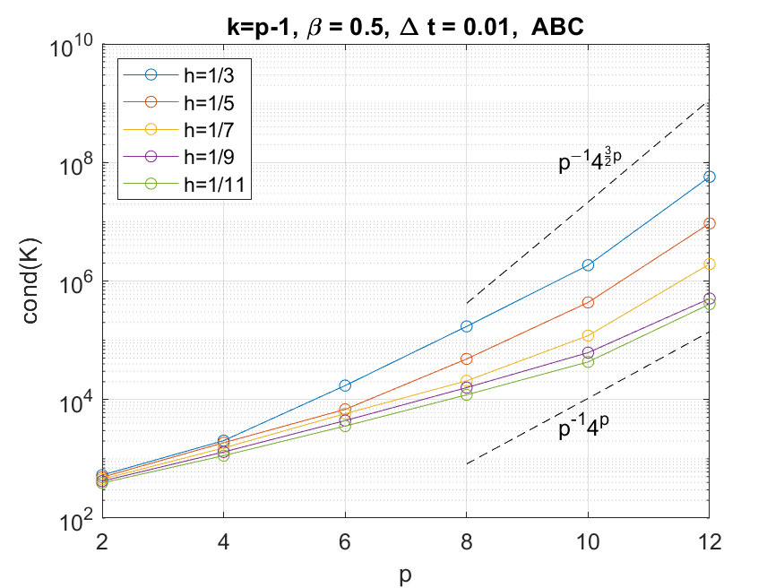
Figure 15: Condition number of the stiffness matrix for the acoustic wave problem with absorbing boundary conditions (4), $\Delta t=0.01$, $\gamma=0.5$, $\beta=0$ (explicit Newmark, left), $\beta=0.5$ (implicit Newmark, right). From the top to the bottom, vs.: (1) $h$, for $p=2,\ 4,\ 6,8,\ 10$, $k=1$; (2) $h$, for $p=2,\ 4,\ 6,8,\ 10$, $k=p-1$; (3) $p$, for $h=1/3,\ 1/5,\ 1/7,\ 1/9$, $k=1$; (4) $p$, for $h=1/3,\ 1/5,\ 1/7,\ 1/9,\ 1/11$, $k=p-1$.

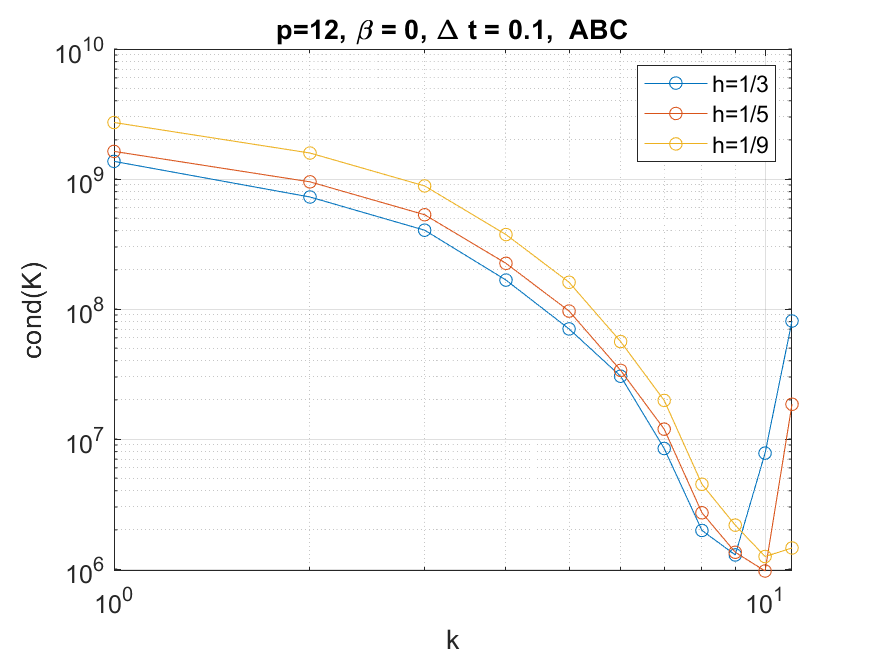
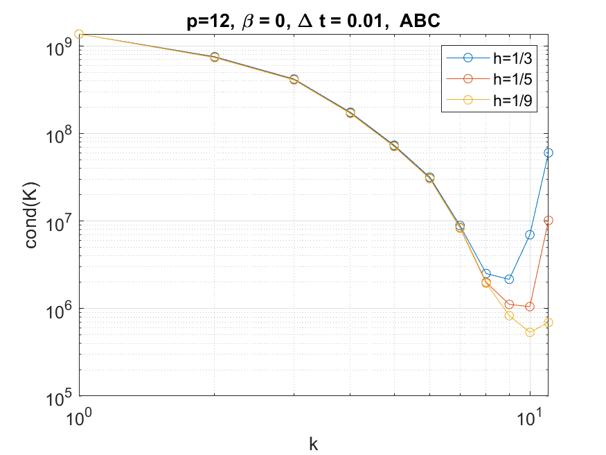
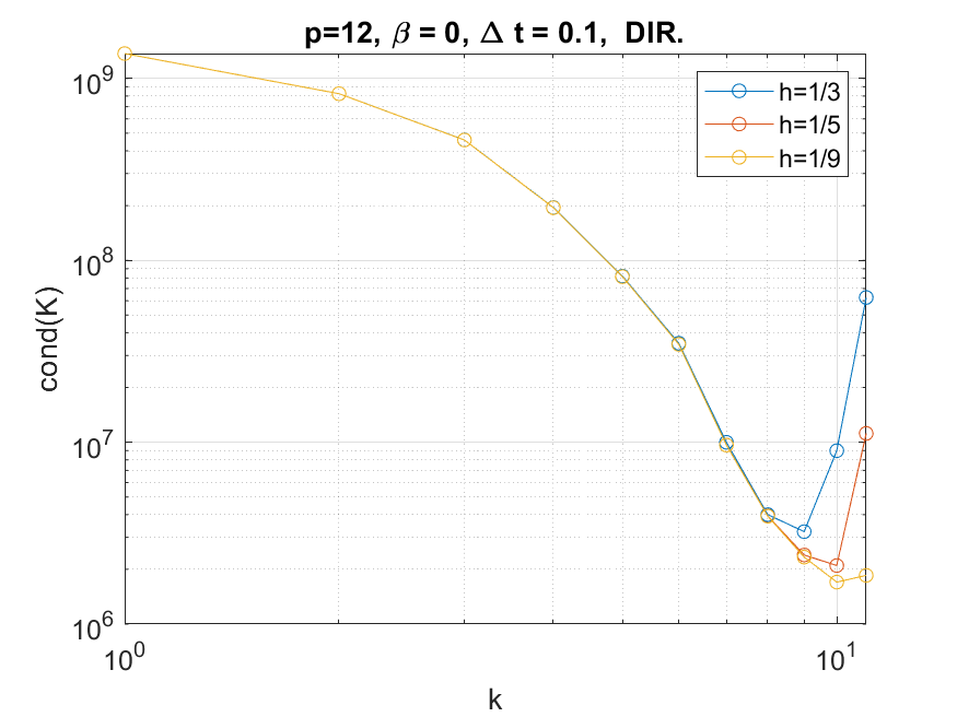
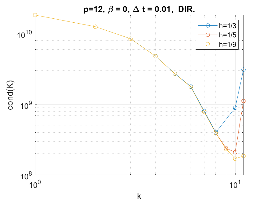
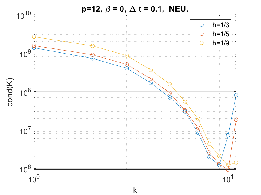
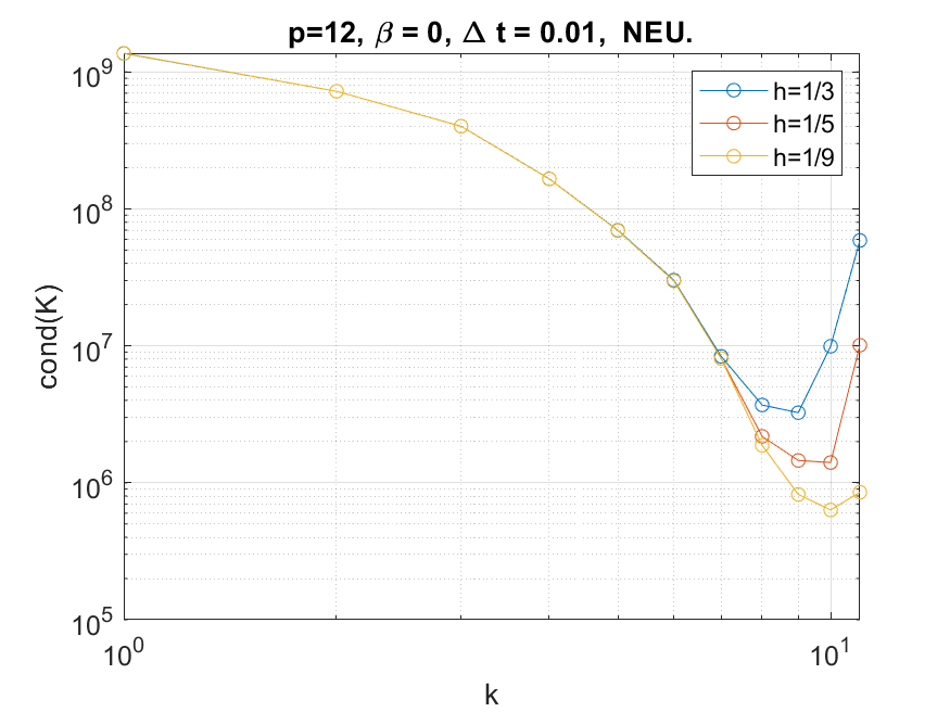
Figure 16: Condition numbers cond($\cal K$) of the stiffness matrix for the acoustic wave problem with different types of boundary conditions: absorbing (top), Dirichlet (center), Neumann (bottom), as a function of $k$, $\beta=0$ (explicit Newmark), $\gamma=0.5$, degree $p=12$, $\Delta t=0.1$ (left) and $\Delta t=0.01$ (right), $h=1/3,\ 1/5,\ 1/9$.

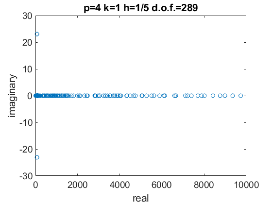
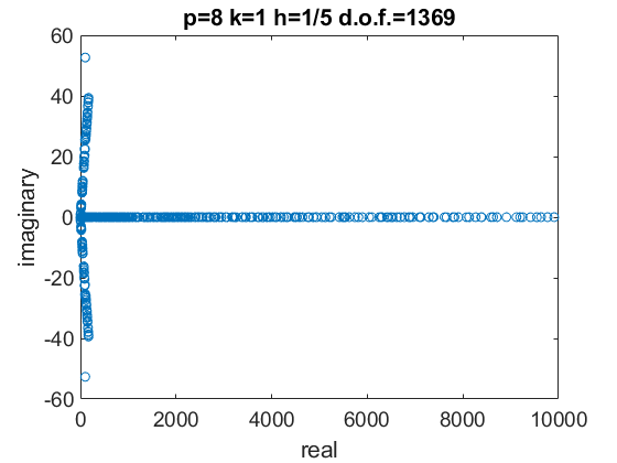
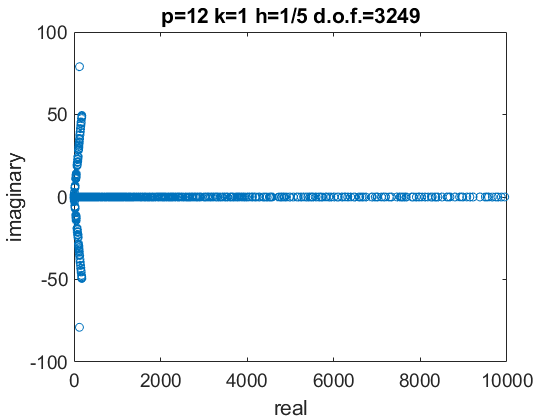
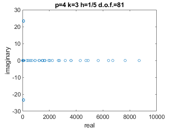
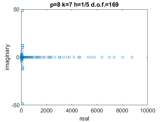
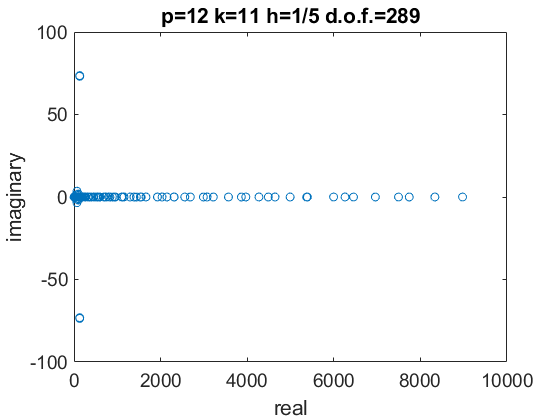
Figure 17: Stiffness matrix eigenvalue distribution in the complex plane for the acoustic wave problem with absorbing boundary conditions and explicit Newmark scheme ($\beta=0)$: $p=4$ (left), $p=8$ (center), $p=12$ (right), with $k=1$ (top) or $k=p-1$ (bottom), fixed $h=1/5$, $\Delta t=0.01$, $\gamma=0.5$.

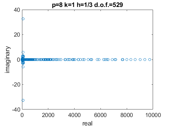
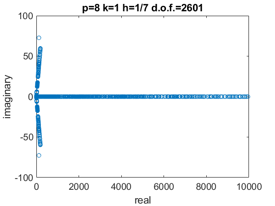
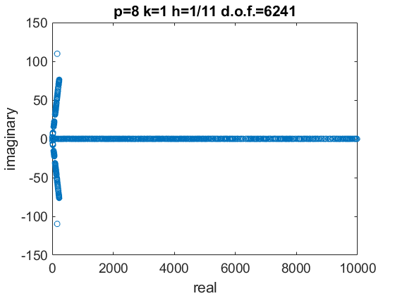
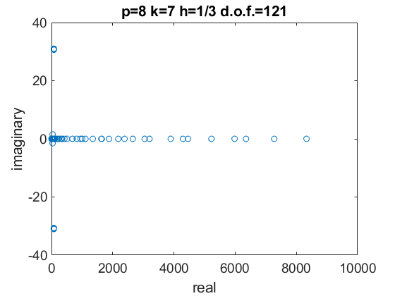
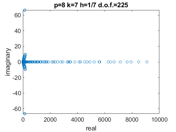
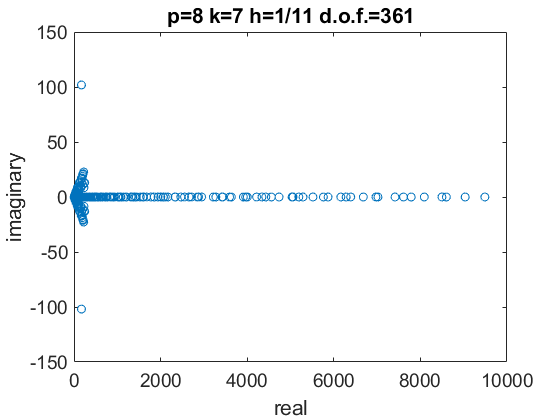
Figure 18: Eigenvalue distribution in the complex plane of stiffness matrix for the acoustic wave problem with absorbing boundary conditions and explicit Newmark scheme ($\beta=0)$: $h=1/3$ (left), $1/h=7$ (center), $1/h=11$ (right), with $k=1$ (top) or $k=p-1$ (bottom), fixed $p=8$, $\Delta t=0.01$, $\gamma=0.5$.

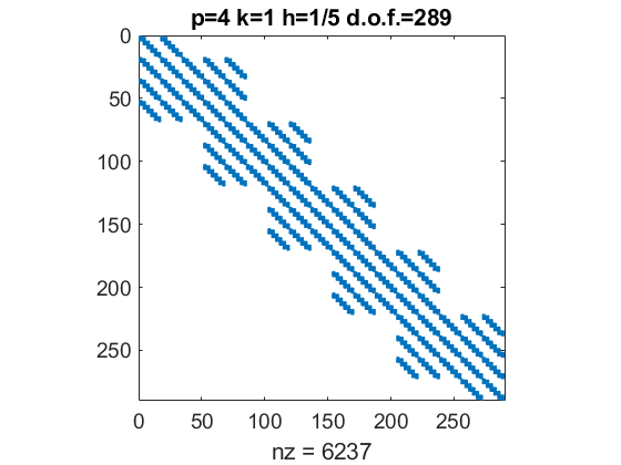
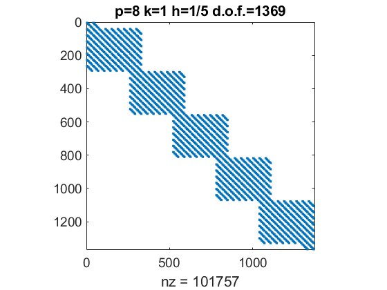
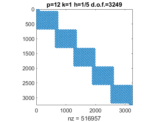
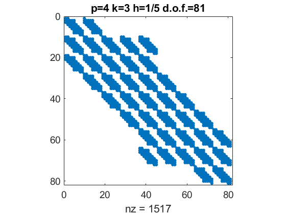
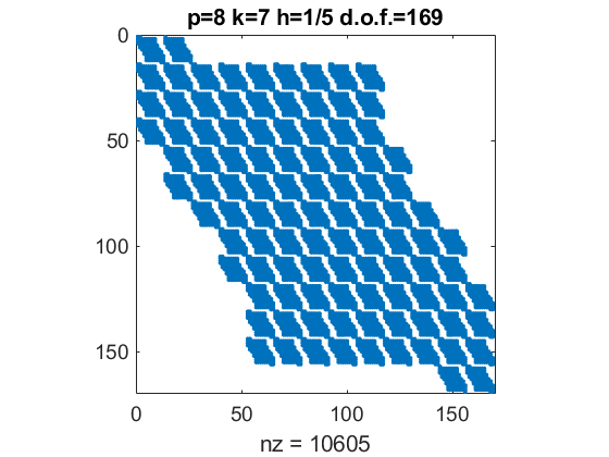
Figure 19: Stiffness matrix sparsity pattern for the acoustic wave problem with absorbing boundary conditions and explicit Newmark scheme ($\beta=0)$: $p=4$ (left), $p=8$ (center), $p=12$ (right), with $k=1$ (top) or $k=p-1$ (bottom), fixed $h=1/5$, $\Delta t=0.01$, $\gamma=0.5$.

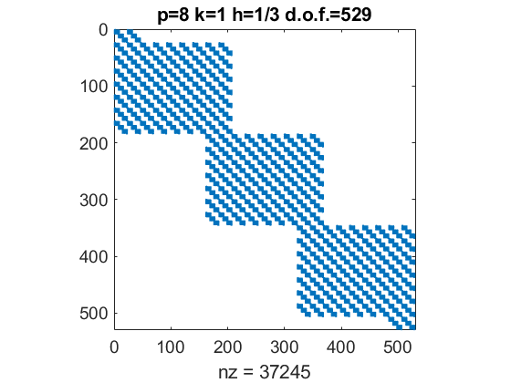
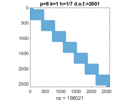
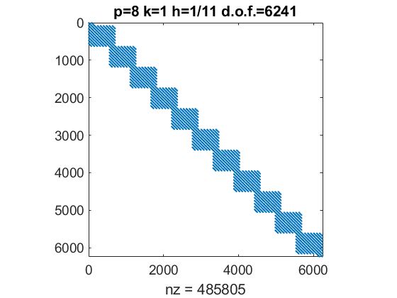
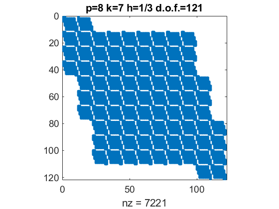
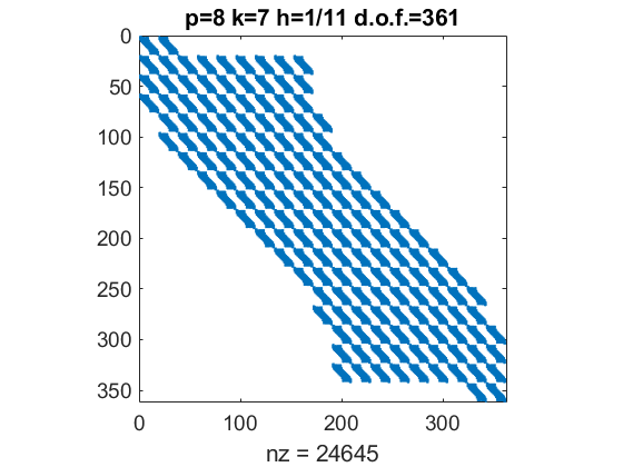
Figure 20: Stiffness matrix sparsity pattern for the acoustic wave problem with absorbing boundary conditions and explicit Newmark scheme ($\beta=0)$: $h=1/3$ (left), $1/h=7$ (center), $1/h=11$ (right), with $k=1$ (top) or $k=p-1$ (bottom), fixed $p=8$, $\Delta t=0.01$, $\gamma=0.5$.

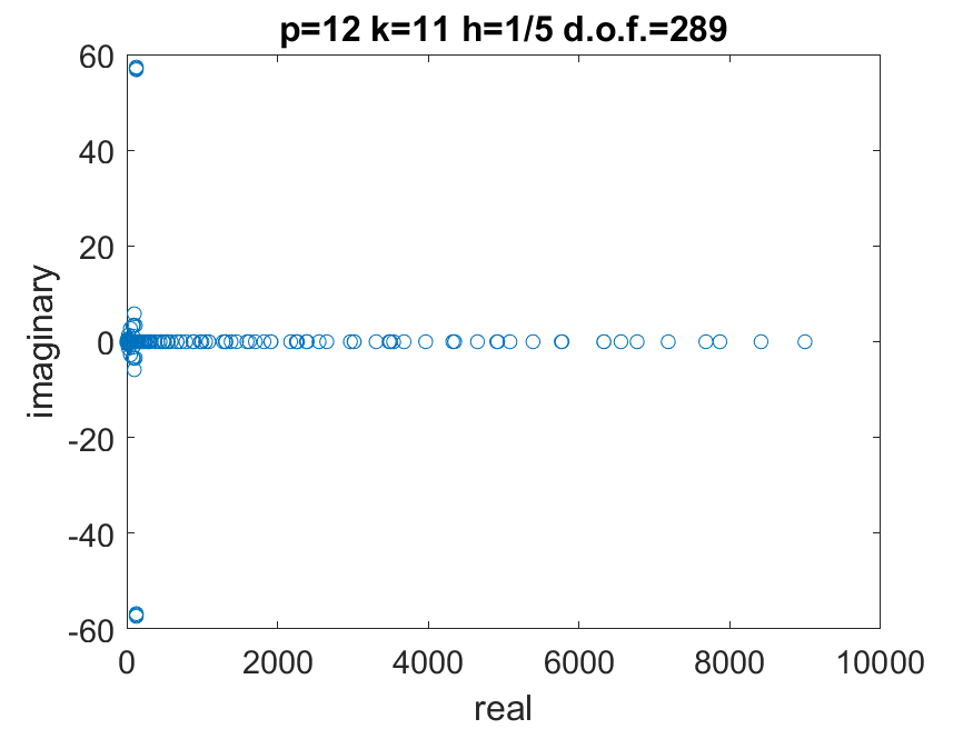
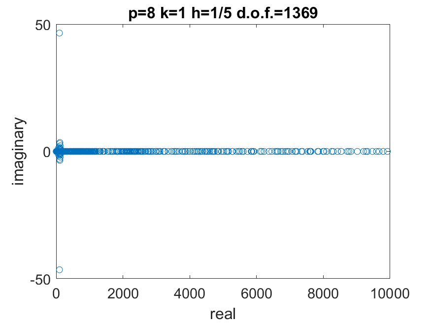
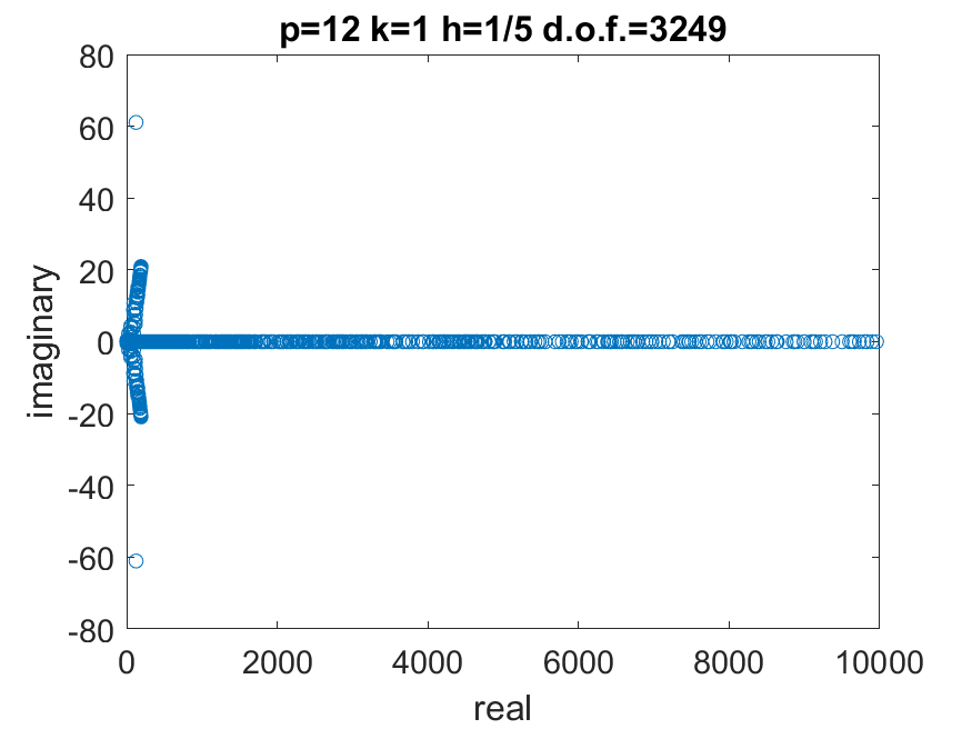
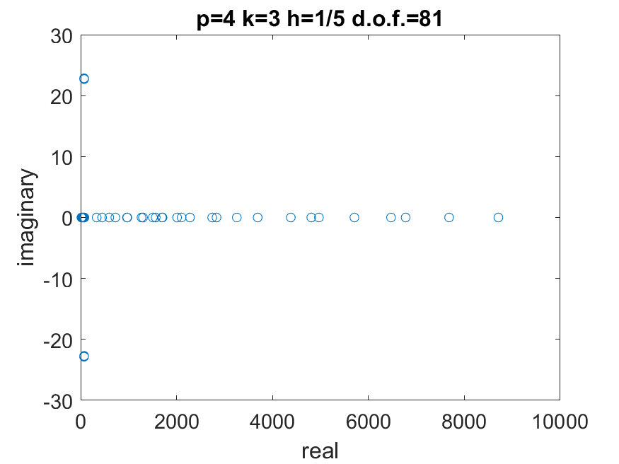
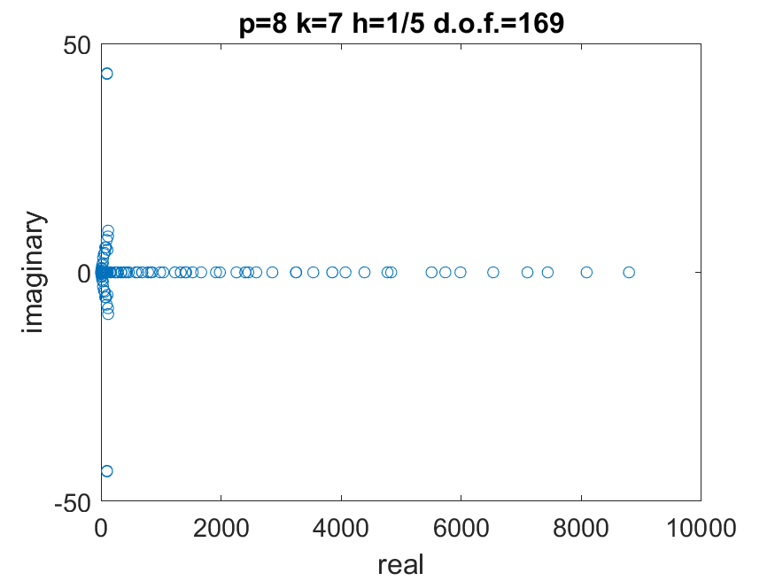
Figure 21: Stiffness matrix eigenvalue distribution in the complex plane for the acoustic wave problem with absorbing boundary conditions and implicit Newmark scheme ($\beta=0.5)$: $p=4$ (left), $p=8$ (center), $p=12$ (right), with $k=1$ (top) or $k=p-1$ (bottom), fixed $h=1/5$, $\Delta t=0.01$, $\gamma=0.5$.

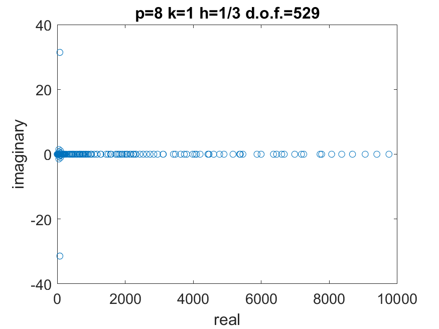
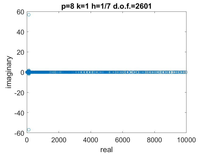
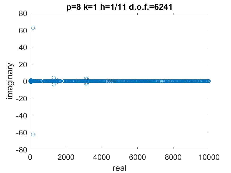
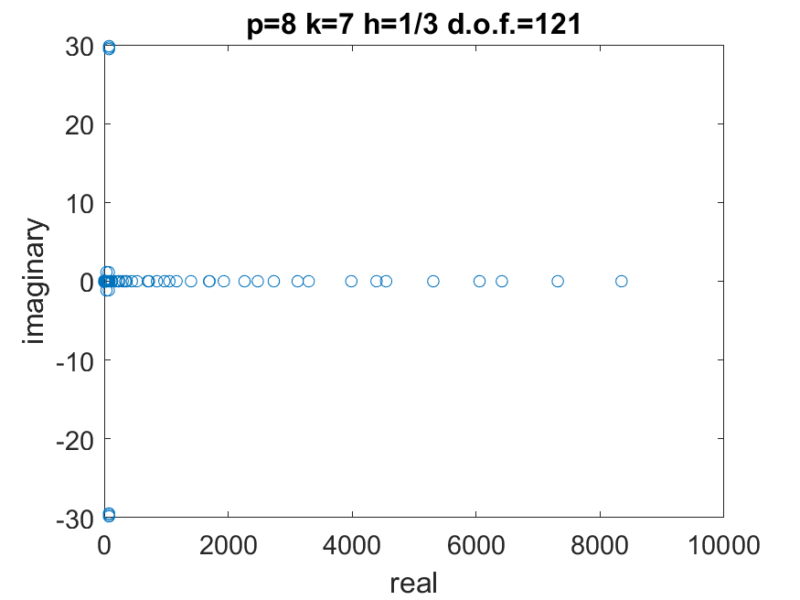
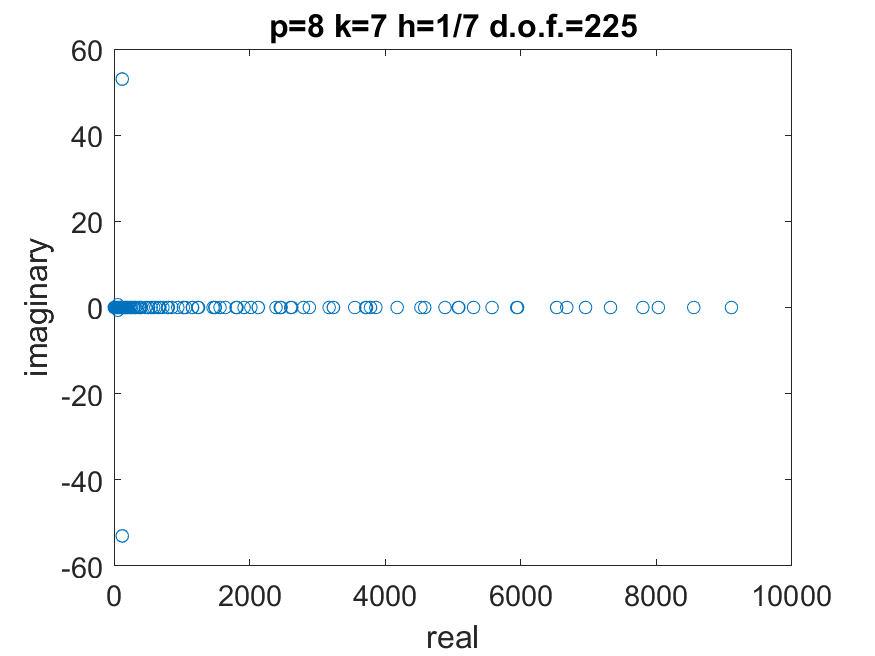
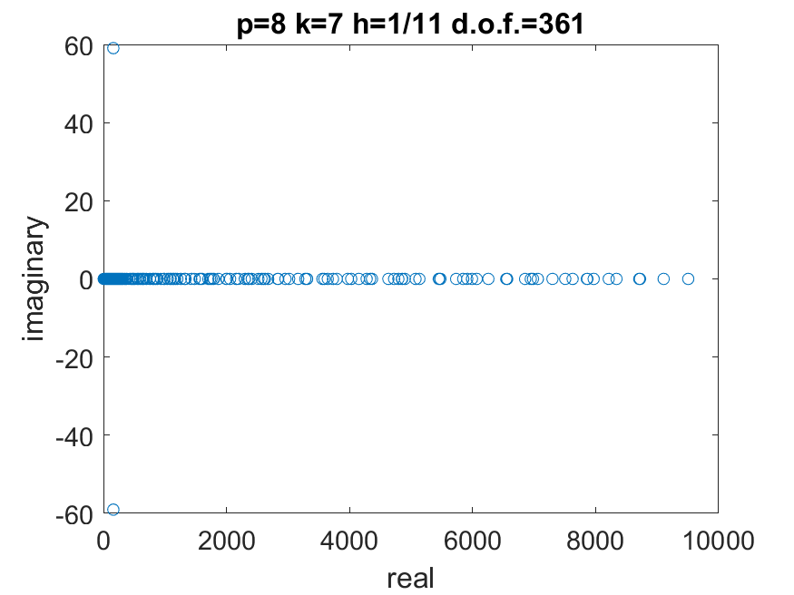
Figure 22: Stiffness matrix eigenvalue distribution in the complex plane for the acoustic wave problem with absorbing boundary conditions and implicit Newmark scheme ($\beta=0.5)$: $h=1/3$ (left), $1/h=7$ (center), $1/h=11$ (right), with $k=1$ (top) or $k=p-1$ (bottom), fixed $p=8$, $\Delta t=0.01$, $\gamma=0.5$.

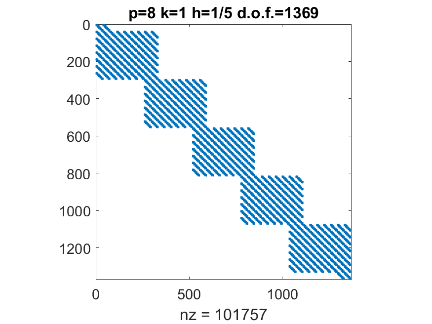
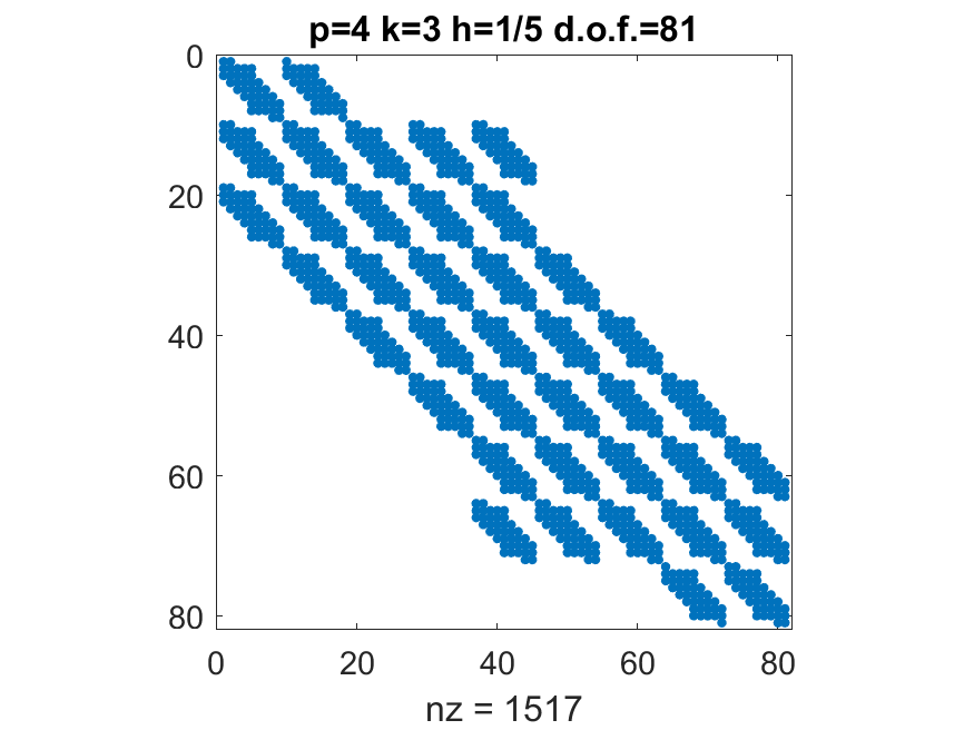
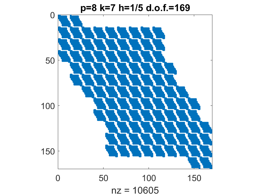
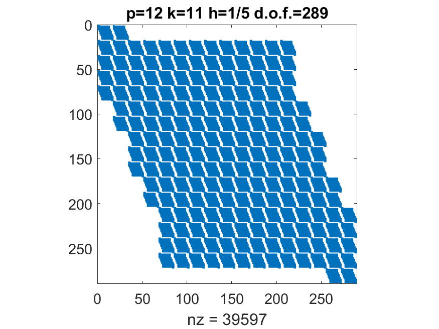
Figure 23: Stiffness matrix sparsity pattern for the acoustic wave problem with absorbing boundary conditions and implicit Newmark scheme ($\beta=0.5)$: $p=4$ (left), $p=8$ (center), $p=12$ (right), with $k=1$ (top) or $k=p-1$ (bottom), fixed $h=1/5$, $\Delta t=0.01$, $\gamma=0.5$.

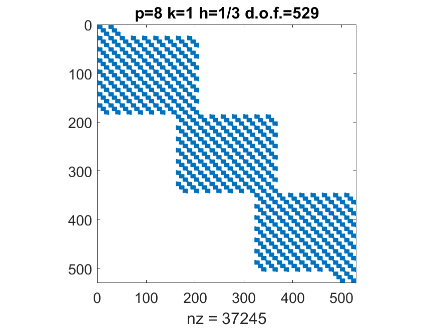
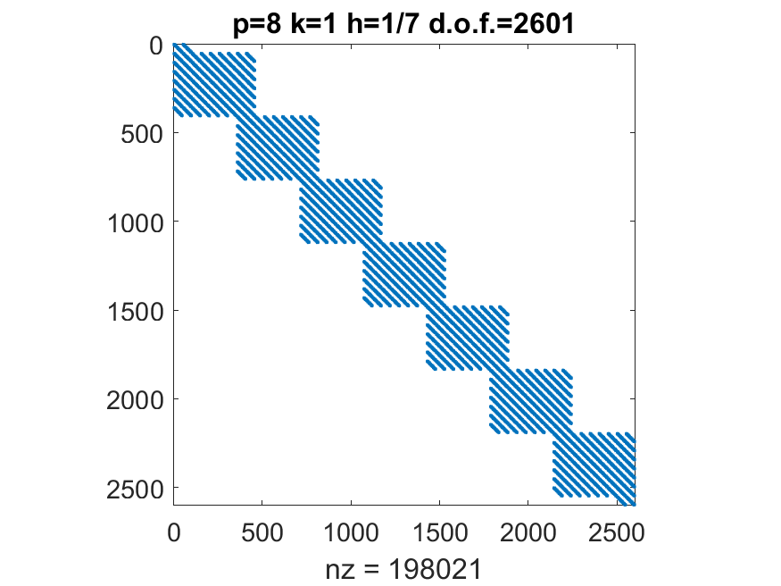
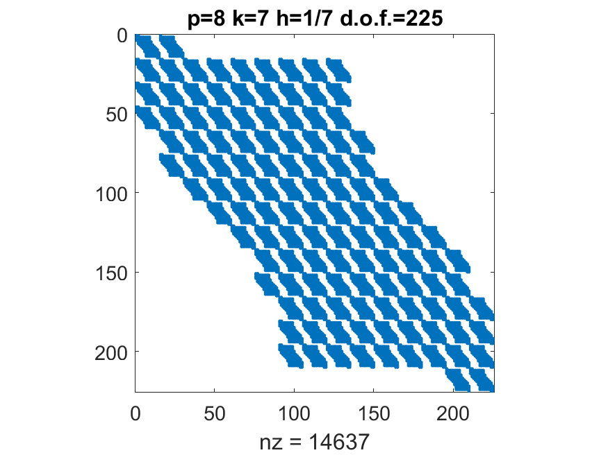
Figure 24: Stiffness matrix sparsity pattern for the acoustic wave problem with absorbing boundary conditions and implicit Newmark scheme ($\beta=0.5)$: $h=1/3$ (left), $1/h=7$ (center), $1/h=11$ (right), with $k=1$ (top) or $k=p-1$ (bottom), fixed $p=8$, $\Delta t=0.01$, $\gamma=0.5$.

6 Conclusions

In this paper we have considered the spectral properties of the mass and stiffness matrices related to the approximation of the acoustic wave equation with Dirichlet, Neumann and absorbing boundary conditions in the reference square domain by IGA collocation methods in space and Newmark advancing schemes in time, both explicit and implicit. Since no theoretical results are yet available in the literature for IGA collocation matrices, we have addressed a systematic numerical study of the eigenvalue distribution, condition numbers and sparsity of the mass and stiffness matrices varying the discretization parameters $p$, $h$, $k$, $\Delta t$, $\beta$, d.o.f. and nz. This analysis is of interest not only in order to estimate the maximum allowable time step $\Delta t$ for explicit Newmark schemes, but also for the possible investigation of efficient preconditioned iterative solutions of the linear systems arising at each step of the time advancing schemes, since the corresponding matrices are full and non-symmetric for both explicit and implicit methods.

Despite the lack of specific collocation bounds and estimates, we have compared some results of our tests with the theory and numerical experiments available for matrices resulting from IGA Galerkin approximation of the Laplacian with Dirichlet boundary conditions. Our results show that analogous estimates for the condition numbers of mass and stiffness matrices hold also for IGA collocation discretizations of acoustic wave problems, and in some case the collocation bounds are better than the Galerkin ones.

Limitations and future work. This study was confined to acoustic wave problems in the reference square, but we do not expect different trends and technical complexity in extending the tests to three dimensional domains, by using the tensor product structure of IGA collocation.
Future work will consider the issue of preconditioning the linear systems arising at each time step, as well as the extension of this work to elastic wave problems.

References

- [1] F. Auricchio, L. Beirão da Veiga, T.J.R. Hughes, A. Reali, G. Sangalli. Isogeometric Collocation Methods. Math. Mod. Meth. Appl. Sci., 20 (11): 2075–2107, 2010.
- [2] F. Auricchio, L. Beirão da Veiga, T.J.R. Hughes, A. Reali, G. Sangalli. Isogeometric collocation for elastostatics and explicit dynamics. Comput. Meth. Appl. Mech. Eng., 249–252: 2–14, 2012.
- [3] Y. Bazilevs, L. Beirão da Veiga, J.A. Cottrell, T.J.R. Hughes, G. Sangalli. Isogeometric analysis: approximation, stability and error estimates for -refined meshes. Math. Mod. Meth. Appl. Sci., 16:1–60, 2006.
- [4] L. Beirão da Veiga, A. Buffa, G. Sangalli, R. Vazquez. Mathematical analysis of variational isogeometric methods. Acta Numer., 157–287, 2014.
- [5] R. Clayton, B. Engquist. Absorbing boundary conditions for acoustic and elastic wave equations. Bull. Seism. Soc. Am., 67(6):1529–1540, 1977.
- [6] J.A. Cottrell, T.J.R. Hughes, Y. Bazilevs. Isogeometric Analysis. Towards integration of CAD and FEA. Wiley, 2009.
- [7] J. Cottrell, A. Reali, Y. Bazilevs, T.J.R. Hughes. Isogeometric Analysis of structural vibrations. Comput. Methods Appl. Mech. Engrg., 195:5257–5296, 2006.
- [8] L. Dedé, C. J aggli, A. Quarteroni. Isogeometric numerical dispersion analysis for two-dimensional elastic wave propagation. Comput. Methods Appl. Mech. Engrg., 284: 320–348, 2015.
- [9] C. De Falco, A. Reali, R. Vazquez. GeoPDEs: a research tool for Isogeometric Analysis of PDEs. Advances in Engineering Software, 42 (12), 1020-1034, 2011.
- [10] C. de Boor. A practical guide to splines. Springer, 2001.
- [11] S. Demko. On the existence of interpolation projectors onto spline spaces, J. of Approx. Theory, 43, 151–156, 1985.
- [12] B. Engquist, A. Majda. Radiation boundary conditions for acoustic and elastic wave equations. Commun. Pure Appl. Math., 32:313–357, 1979.
- [13] J. A. Evans, R. R. Hiemstra, T. J. R. Hughes, A. Reali. Explicit higher-order accurate isogeometric collocation methods for structural dynamics. Comput. Methods Appl. Mech. Engrg., 338(15): 208–240, 2018.
- [14] K. Gahalaut, S. Tomar. Condition number estimates for matrices arising in the isogeometric discretization. Tech. Report 2012-23, RICAM, 2012.
- [15] C. Garoni, C. Manni, F. Pelosi, S. Serra Capizzano, H. Speelers. On the spectrum of stiffness matrices arising from isogeometric analysis. Numer. Math. 127 (4): 751–799, 2014.
- [16] P. Gervasio, L. Dedé, O. Chanon, A. Quarteroni. A computational comparison between Isogeometric Analysis and Spectral Element Methods: accuracy and spectral properties. J. Sci. Comp., 83:1–45, 2020.
- [17] D. Givoli. Non-reflecting boundary conditions. J. Comput. Phys., 94(1):1–29, 1991.
- [18] H. Gomez, L. De Lorenzis. The variational collocation method. Comput. Methods Appl. Mech. Engrg., 309: 152–181, 2016.
- [19] T.J.R. Hughes, J.A. Cottrell, Y. Bazilevs. Isogeometric analysis: CAD, finite elements, NURBS, exact geometry, and mesh refinement. Comp. Meth. Appl. Mech. Engrg., 194, 4135–4195, 2005.
- [20] T.J.R. Hughes, A. Reali, G. Sangalli. Isogeometric methods in structural dynamics and wave propagation. In COMPDYN 2009, M. Papadrakakis et al. (eds.), 2009.
- [21] F. Ihlenburg. Finite element analysis of acoustic scattering. Applied Mathematical Sciences, 132. Springer-Verlag, Berlin, 1998.
- [22] M. C. Junger, D. Feit. Sound, Structures and their Interaction. MIT Press, Cambridge, MA, 1986.
- [23] D. Komatitsch, J. Ritsema, J. Tromp. Accurate solutions of wave propagation problems under impact loading by the standard, spectral and isogeometric high-order finite elements. Comparative study of accuracy of different space-discretization techniques. Finite Elem. Anal. Des., 88 : 67–89, 2014.
- [24] G. Loli, G. Sangalli, M. Tani. Easy and efficient preconditioning of the isogeometric mass matrix. Comput. Math. Appl., 2022, to appear.
- [25] R. Kruse, N. Nguyen-Thanh, L. De Lorenzis, T.J.R. Hughes. Isogeometric collocation for large deformation elasticity and frictional contact problems. Comp. Meth. Appl. Mech. Engrg., 296, 73–112, 2015.
- [26] M. Montardini, G. Sangalli, L. Tamellini. Optimal-order isogeometric collocation at Galerkin superconvergent points, Comput. Methods Appl. Mech. Engrg., 316: 741–757, 2017.
- [27] G. Mur. Absorbing boundary conditions for the finite–difference approximation of the time-domain electromagnetic–field equations. IEEE Trans. Elect. Compat., 23(4):377–382, 1981.
- [28] N. M. Newmark. A method of computation for structural dynamics. Proceedings of ASCE, Journal of Engineering Mechanics (EM3), 85:67–94, 1959.
- [29] A. Quarteroni, A. Tagliani, E. Zampieri. Generalized Galerkin approximations of elastic waves with absorbing boundary conditions. Comput. Methods Appl. Mech. Engrg., 163:323–341, 1998.
- [30] D.F. Rogers. An Introduction to NURBS With Historical Perspective. Academic Press, 2001.
- [31] L.L. Schumaker. Spline Functions: Basic Theory. 3rd Edition, Cambridge Mathematical Library, Cambridge University Press, Cambridge, 2007.
- [32] D. Schillinger, J. A. Evans, A Reali, M. A. Scott, T. J.R. Hughes. Isogeometric Collocation: cost comparison with Galerkin methods and extension to adaptive hierarchical NURBS discretizations. Comp. Meth. Appl. Mech. Engrg., 267:170–232, 2013.
- [33] R. Vazquez. A new design for the implementation of isogeometric analysis in Octave and Matlab: GeoPDEs 3.0. IMATI REPORT Series 16-02, 2016.
- [34] W. L. Wood. A further look at Newmark, Houbolt, etc., time-stepping formulae. Int. J. Numer. Meth. Engrg., 20: 1009–1017, 1984.
- [35] W. L. Wood. Practical time-stepping schemes. Clarendon Press, Oxford, 1990.
- [36] E. Zampieri, L. F. Pavarino. Explicit second order isogeometric discretizations for acoustic wave problems. Comput. Methods Appl. Mech. Engrg., 348: 776–795, 2019.
- [37] E. Zampieri, L. F. Pavarino. Isogeometric collocation discretizations for acoustic wave problems. Comput. Methods Appl. Mech. Engrg., 385: 114047, 2021.
- [38] S. Zhu, L. Dedé, A. Quarteroni. Isogeometric analysis and proper orthogonal decomposition for the acoustic wave equation. ESAIM: Math. Meth. Numer. Anal., 51: 1197–1221, 2017.