Topological superconductivity from doping a triplet quantum spin liquid in a flat band system

Abstract

We explore superconductivity in strongly interacting electrons on a decorated honeycomb lattice (DHL). An easy-plane ferromagnetic interaction arises from spin-orbit coupling in the Mott insulating phase, which favors a triplet resonance valence bond spin liquid state. Hole doping leads to partial occupation of a flat band and to triplet superconductivity. The order parameter is highly sensitive to the doping level and the interaction parameters, with $p+ip$, $f$ and $p+f$ superconductivity found, as the flat band leads to instabilities in multiple channels. Typically, first order transitions separate different superconducting phases, but a second order transition separates two time reversal symmetry breaking $p+ip$ phases with different Chern numbers ($\nu=0$ and 1). The Majorana edge modes in the topological ($\nu=1$) superconductor are almost localized due to the strong electronic correlations in a system with a flat band at the Fermi level. This suggests that these modes could be useful for topological quantum computing. The ‘hybrid’ $p+f$ state does not require two phase transitions as temperature is lowered. This is because the symmetry of the model is lowered in the $p$-wave phase, allowing arbitrary admixtures of $f$-wave basis functions as overtones. We show that the multiple sites per unit cell of the DHL, and hence multiple bands near the Fermi energy, lead to very different nodal structures in real and reciprocal space. We emphasize that this should be a generic feature of multi-site/multi-band superconductors.

I Introduction

Understanding the mechanism of superconductivity in strongly correlated materials remains a formidable challenge. For instance, high-$T_{c}$ cuprates [1, 2, 3], organics[4] and twisted bilayer graphene [5, 6] (TBG), display similar phase diagrams[7]. In these materials superconductivity emerges near to a Mott insulating phase, indicating the important role played by strong correlations on Cooper pairing. A common ingredient in these systems is the presence of antiferromagnetic interactions, which lead to Mott insulators with antiferromagnetic order, as in the cuprates, or quantum spin liquids, as in the organic materials $\kappa$-(BEDT-TTF)₂Cu(CN)₃ or $\kappa$-(BEDT-TTF)₂Ag(CN)₃ [8, 9, 4]. Such AF interaction is crucial to singlet $d$-wave (or $d+id$) superconductivity which, according to Andersons theory of high-$T_{c}$ superconductivity [10], can emerge when hole doping the resonance valence bond (RVB) Mott insulator on the square (triangular [11]) lattice [12]. The discovery of superconductivity in magic angle TBG [6] poses new questions about strongly correlated superconductivity in flat bands [13].

Definitive signatures of triplet pairing are rare outside the well understood triplet superfluidity [14, 15] in ³He. At present, there is no unambiguous evidence for, and increasing evidence against, triplet pairing in (former) candidate materials such as Sr₂RuO₄ [16, 17, 18], the quasi-one-dimensional (TMTSF)₂X Bechgaard salts[19] or A₂Cr₃As₃ [20, 21], (A=K, Rb, Cs). A reason for the scarcity of triplet superconductors is the antiferromagnetic (AFM) superexchange between spins which often dominates over ferromagnetic exchange processes, likely to stabilize triplet superconductivity. However, the superconductivity observed [22] in the ferromagnetic Mott insulators, CrXTe₃ with $X=$Si, Ge has been predicted to be of the triplet type [23]. Perhaps the most promising class of materials for observing triplet superconductors are the uranium based heavy fermion materials [24, 25], where superconductivity is often found near ferromagnetism.

Quantum spin liquids with ferromagnetic interactions cannot be described through standard singlet RVB theory. However, recent extensions to easy-plane ferromagnetic triangular lattices predict the existence of triplet resonance valence bond (tRVB) Mott insulators which can become unconventional $p+ip$-wave superconductors under hole doping[23]. On the other hand, in multiorbital systems such as the iron pnictides, Hunds coupling can induce an intra-atomic triplet RVB state [26]. In these cases, triplet superconductivity may arise under hole doping. This is allowed by the presence of an even number of atoms per unit cell, leading to a spatially staggered gap pattern, as proposed by Anderson [27] in the context of heavy fermion superconductivity.

Triplet pairing induced by ferromagnetic interactions may arise in certain organic and organometallic materials with unit cells containing many atoms. (EDT-TTF-CONH₂)₆[Re₆Se₈(CN)₆] [28], Mo₃S₇(dmit)₃ [29], and Rb₃TT$\cdot$2H₂O [30] crystals with layers of decorated honeycomb lattices (DHLs) can potentially host rich physics arising from the interplay of strong correlations, Dirac points, quadratic band touching points and flat bands [31, 32, 33, 34, 35]. This lattice also occurs in several metal organic frameworks and coordination polymers [35]. Indeed, unconventional singlet $f$-wave pairing has been found in an AFM $t$-$J$ model on the DHL [36]. However, the spin molecular-orbital coupling (SMOC) present in these systems,[37, 38, 39, 40] can lead to easy-plane ferromagnetic interactions favoring tRVB states. Hence, it is interesting to address the question of whether triplet superconductivity emerges in a strongly correlated easy-plane ferromagnetic model on a DHL. The possibility of finding non-trivial topological superconductivity as well as the role played by the flat bands deserve special attention.

In this paper we study a $t$-$J$ model on a DHL with XXZ interactions, which arise due to spin-orbit coupling. Exact diagonalization of small clusters shows that a tRVB spin liquid, is a competitive ground state of the model at half-filling. Hole doping this spin liquid state leads to partial occupation of a flat band. Based on this we apply the tRVB approach to search for superconductivity in the hole doped system. We find multiple triplet superconducting phases, including include $p+ip$, $p+f$, $f$. Presumably, the wide variety of superconducting phases is a consequence of the flat band leading to instabilities in multiple Cooper channels.

Interestingly, we find both topologically trivial and topological $p+ip$ superconductivity with Chern numbers, $\nu=0$ and 1 respectively. These phases are separated by a continuous phase transition, where nodes appear in the otherwise fully gapped $p+ip$ order parameter. In the topological superconductor phase the single Majorana edge mode expected for $\nu=1$ is almost localized since it traverses a tiny gap bounded by nearly flat bands.

We show that the $p+f$ state does not require a two superconducting phase transitions as the temperature is lowered. Rather the once the symmetry of the system is lowered by going into the $p$-wave superconducting phase, the $p$ and $f$ solutions belong to the same irreducible representation of the group describing the symmetry of the model. Therefore, $p$ and $f$ are overtones and the system can and does take advantage of this to lower its energy.

The DHL lattice has six sites per unit cell. Therefore, diagonalizing the Hamiltonian requires a Bogoliubov transformation, a Fourier transformation and a transformation from the multi-site basis to a multiband basis. We show that the latter leads to remarkably different nodal structures in real and reciprocal space. We emphasize that this is a very general phenomenon in multi-band superconductors.

We show that, at strong coupling (low doping), where the magnetic exchange is dominant, real space pairing dominates, leading to order parameters that are fully gapped or have only isolated nodal points in reciprocal space. In contrast, at weak coupling (high doping), where the superconductivity is dominated by the kinetic energy, the superconducting gap displays nodal points in reciprocal space.

The paper is organized as follows: in Sec II we introduce the anisotropic $t$-$J$ model on a DHL with XXZ magnetic exchange interactions. In Sec. III we show, using exact diagonalization of small clusters, that a tRVB spin liquid, is a competitive ground state of the model at half-filling. In Sec. IV we show that a wide variety triplet superconducting states emerge on hole-doping the tRVB, including a topological superconductor (TSC), and give a detailed characterization of these states. In Sec. V we characterize the TSC by calculating the topological invariants and Majorana edge modes. Finally, in Sec. VI we conclude our work by summarizing our main results and their relevance to actual materials realizing DHLs.

II Model

Our starting point is a $t$-$J$ model with easy-plane XXZ ferromagnetic exchange on the DHL:

$${\cal H} = -t\sum_{\alpha ij\sigma}P_{G}\left(c^{\dagger}_{\alpha i\sigma}c_{\alpha j,\sigma}+c^{\dagger}_{\alpha j\sigma}c_{\alpha i\sigma}\right)P_{G}$$ (1)

$$- t^{\prime}\sum_{\begin{subarray}{c}\langle A,B\rangle i\sigma\end{subarray}}P_{G}\left(c^{\dagger}_{Ai\sigma}c_{Bi\sigma}+c^{\dagger}_{Bi\sigma}c_{Ai\sigma}\right)P_{G}$$

$$- J\sum_{\alpha ij}\left(S^{x}_{\alpha i}S^{x}_{\alpha j}+S^{y}_{\alpha i}S^{y}_{\alpha j}-S^{z}_{\alpha i}S^{z}_{\alpha j}+{\frac{1}{4}}n_{\alpha i}n_{\alpha j}\right)$$

$$- J^{\prime}\sum_{\begin{subarray}{c}\langle A,B\rangle i\end{subarray}}\left(S^{x}_{Ai}S^{x}_{Bi}+S^{y}_{Ai}S^{y}_{Bi}-S^{z}_{Ai}S^{z}_{Bi}+{\frac{1}{4}}n_{Ai}n_{Bi}\right)$$

$$+ \mu\sum_{\alpha i\sigma}c^{\dagger}_{\alpha i\sigma}c_{\alpha i\sigma},$$

where $P_{G}=\Pi_{i}(1-n_{i\uparrow}n_{i\downarrow})$ is the Gutzwiller projection operator which excludes doubly occupied sites completely, $c^{(\dagger)}_{\alpha i\sigma}$ is the usual annihilation (creation) operator, and $S^{r}_{\alpha i}$ is the $r$th component of the spin operator. The $\alpha$-index runs over the two triangular clusters, while $i,j$ run over the three sites within each triangular clusters, with site numbering as illustrated in Fig. 1, and $\sigma$ denotes the spin of the electron. Angled brackets indicate that the sums are restricted to (triangles that contain) nearest-neighbor sites. We are interested in the properties of the model close to half-filling, so we write the electron density $n=1-\delta$, where $\delta$ is the density of holes doped into the half-filled DHL. We fix $t=1$ as the energy scale. The XXZ exchange couplings, $J,J^{\prime}>0$, lead to easy-plane ferromagnetic (FM) interactions and AFM longitudinal interaction.

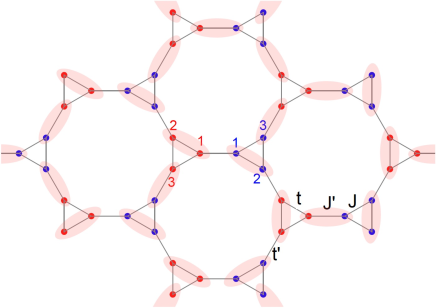
Figure 1: The $t$-$J$ model on the decorated honeycomb lattice. The unit cell consists of a A (red) and a B (blue) triangles with the sites numbered as shown. The parameters entering the model are illustrated. A particular triplet covering of the lattice entering the $|\text{tRVB}\rangle$ state of the model is shown.

A possible microscopic origin of the XXZ exchange interactions of model (1) can be found by considering a single s-like orbital with on site (Hubbard) interactions and SMOC. On transforming to real space SMOC is equivalent to an anisotropic Kane-Mele spin-orbit coupling. If we consider nearest neighbor (nn) interactions with a $z$ component of the spin-orbit coupling only we have

$$\mathcal{H}=i\lambda\sum_{\langle\alpha i\beta j\rangle}(c_{\alpha i\uparrow}^{\dagger}c_{\beta j\uparrow}-c_{\alpha i\downarrow}^{\dagger}c_{\beta j\downarrow})+U\sum_{i\alpha}n_{i\alpha\uparrow}n_{i\alpha\downarrow},$$ (2)

where $n_{i\alpha\sigma}=c_{i\alpha\sigma}^{\dagger}c_{i\alpha\sigma}$. In the large-$U$ limit, the Hubbard model maps onto an effective XXZ spin hamiltonian [41]

$$\mathcal{H}_{\text{XXZ}}=-{\frac{4\lambda^{2}}{U}}\sum_{\langle\alpha i\beta j\rangle}\left(S^{x}_{\alpha i}S^{x}_{\beta j}+S^{y}_{\alpha i}S^{y}_{\beta j}-S^{z}_{\alpha i}S^{z}_{\beta j}\right).$$ (3)

At half-filling, the Hubbard model (2) with $U\gg|\lambda|$ becomes an XXZ model with $J=4\lambda^{2}/U,J^{\prime}=4\lambda^{\prime 2}/U$, i.e. Eq. (1), as is corroborated by our exact denationalization (ED) calculations of Appendix D. On including direct the hopping terms $t$ and $t^{\prime}$ additional AFM exchange, Dzyaloshinskii-Moriya, and off diagonal exchange interactions will be introduced [37, 42, 43]. We neglect these interactions for simplicity. Thus Eq. (1) is a toy model for understanding the impact of SMOC on superconductivity. We further assume that $\lambda\propto t$ and $\lambda^{\prime}\propto t^{\prime}$ so that $J^{\prime}/J=(t^{\prime}/t)^{2}$ reducing the number of independent parameters in our Eq. (1). Other mechanisms for easy-plane ferromagnetic interaction have also been put forward recently, including interactions arising from the interplay of Hund’s and Kondo interactions in heavy fermions.[44]

We emphasize that different materials are known to span a wide range of the parameter space for this model. For example, in Mo₃S₇(dmit)₃ is in the trimerized limit: $t^{\prime}<t$ and $J^{\prime}<J$ [45, 38], whereas in (EDT-TTF-CONH₂)₆[Re₆Se₈(CN)₆] [28] and Rb₃TT$\cdot$2H₂O [30] are in the dimerized limit: $t^{\prime}>t$ and $J^{\prime}>J$. The physics of these two limits is known to differ markedly [32, 35]. Furthermore, at ambient pressure, (EDT-TTF-CONH₂)₆[Re₆Se₈(CN)₆] undergoes a metal-insulator transition as the temperature is lowered [28], whereas Mo₃S₇(dmit)₃ [29] and Rb₃TT$\cdot$2H₂O [30] are insulating at all temperatures at ambient pressure.

III Triplet RVB quantum spin liquid

We analyze the ground state of model (1) by using tRVB theory[46], which has recently applied to iron pnictides[26] and transition metal chalcogenides[23]. It is analogous to Andersons RVB theory of high-$T_{c}$ superconductivity to deal with strongly correlated models containing ferromagnetic exchange. Triplets rather than singlet bonds are the building blocks of the theory. The simplest form of the theory assumes that the ground state of the ferromagnetic undoped model is a quantum spin liquid in which spins are paired into triplets.

In general, such triplet RVB state can be expressed as:

$$|\text{tRVB}\rangle=\sum_{P}A_{P}|P_{t}\rangle,$$ (4)

where $|P_{t}\rangle=\Pi_{{ij}\in P}|ij\rangle$ and the $S_{z}=0$ spin triplet between sites $i,j$ is

$$|ij\rangle\equiv\frac{|i,\uparrow\rangle|j,\downarrow\rangle+|i,\downarrow\rangle|j,\uparrow\rangle}{\sqrt{2}},$$ (5)

where $|ij\rangle=-|ji\rangle$ due to the symmetry of triplets under inversion. Hence, the $|t\text{RVB}\rangle$ state is a quantum superposition of all possible coverings of the lattice into triplet valence bonds. The simplest version of the $|t\text{RVB}\rangle$ state involves triplets between nn spins only. One possible snapshot triplet configuration $|P_{t}\rangle$ entering $|t\text{RVB}\rangle$ is shown in Fig. 1.

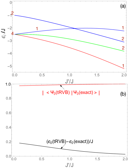
Figure 2: Exact triplet RVB analysis of the half-filled easy-axis XXZ ferromagnetic model on a six site (two triangle) cluster. (a) The dependence of the low energy spectrum of the model (1) on $J^{\prime}/J$. The numbers denote the exact energy level degeneracies. (b) The overlap between the exact ground state and the tRVB wavefunction for the six site cluster (given in Eq. (LABEL:eq:varRVB)), $|\langle\Psi_{0}(\text{tRVB})|\Psi_{0}(\text{exact})\rangle|$, and the difference between the exact ground state energy, $\epsilon_{0}(\text{exact})$, and the triplet RVB energy, $\epsilon_{0}(\text{tRVB})$.

III.1 Exact analysis of the triplet RVB in the DHL

We first concentrate on model (1) at half-filling, $\delta=0$, which becomes a easy-plane XXZ ferromagnetic model. Triplet RVB states in such spin model are explored by performing exact diagonalization on six-site (two-triangle) clusters. The dependence of the exact level spectra of the cluster with $J^{\prime}/J$ is shown in Fig. 2(a). For any $J^{\prime}/J\neq 0$ the four-fold ground state degeneracy found at $J^{\prime}=0$ is split so that the ground state becomes a non-degenerate $S=1,S_{z}=0$ triplet, as expected. The first excitation corresponds to a $S=1,S_{z}=\pm 1$ doublet. The splitting between the $S=1,S_{z}=0$ and $S=1,S_{z}=\pm 1$ states is increased by $J^{\prime}/J$. The ground state energy at $J^{\prime}=J$ is $\epsilon_{0}(\text{exact})=-3.541287J$, and the corresponding wavefunction is given in the Appendix. B.

We now consider a simple nn tRVB ansatz for the ground state wavefunction of the cluster, which consists on a linear combination of nn triplet valence bonds (VB) only:

$$|\text{tRVB}\rangle = |{A1B1}\rangle|{A2A3}\rangle|{B2B3}\rangle+|{A1A3}\rangle|{A2B2}\rangle|{B1B3}\rangle$$

$$+|{A1A2}\rangle|A3B3\rangle|B1B2\rangle-|A1B1\rangle|{A2B2}\rangle|{A3B3}\rangle,$$

with the corresponding energy

$$\epsilon_{0}(\text{nn-tRVB})={\langle\text{nn-tRVB}|\cal{H}_{\text{XXZ}}|\text{nn-tRVB}\rangle\over\langle\text{nn-tRVB}|\text{nn-tRVB}\rangle}.$$ (7)

For $J^{\prime}=J$ the overlap with the exact ground state is $\langle\Psi_{0}(\text{exact})|\text{nn-tRVB}\rangle=0.9747$, its energy is $\epsilon_{0}(\text{nn-tRVB})=-3.397058J$ which is $4.07\%$ higher than the exact ground state energy. In contrast, an RVB analysis of the Heisenberg antiferromagnetic model on the same cluster using nn singlet VBs would give a much more accurate description of the exact ground state: $\langle\Psi_{0}^{\text{HAFM}}(\text{exact})|\text{nn-RVB}\rangle=0.9988$ and $\epsilon^{HAFM}_{0}(nn-\text{RVB})=-3.04412J$. The energy of this RVB state is only $0.16\%$ higher than the exact ground state energy, $\epsilon^{HAFM}_{0}(\text{exact})=-3.052775J$. Hence, it appears that the nn RVB gives a much better description of the ground state of the AFM Heisenberg model than the nn-tRVB of the easy-plane XXZ magnetic exchange we consider in this work.

We therefore consider a more general nn tRVB ansatz:

$$|\text{tRVB}\rangle=\alpha\left(|A1B1\rangle|A2A3\rangle|B2B3\rangle+|A1A3\rangle|A2B2\rangle|B1B3\rangle\right.$$

$$\left.+|A1A2\rangle|A3B3\rangle|B1B2\rangle\right)-\beta|A1B1\rangle|A2B2\rangle|A3B3\rangle,$$

where $\alpha$ and $\beta$ are determined variationally. For $J^{\prime}=J$ we find an energy of $\epsilon_{0}(\text{tRVB})=-3.453257J$ which is only $2.5\%$ higher than the exact ground state energy. The overlap with the exact wavefunction is now $\langle\Psi_{0}(\text{exact})|\text{tRVB}\rangle=0.98849$, improving our previous result. For comparison a singlet-RVB version of (LABEL:eq:varRVB) for the Heisenberg antiferromagnet (HAF) recovers its exact ground state, i.e., $\langle\text{RVB}|\Psi^{\text{AFM}}_{0}(\text{exact})\rangle=1$, with an energy $\epsilon_{0}(\text{RVB})=\epsilon^{\text{AFM}}_{0}(\text{exact})=-5.302775J$.

short name	$\Gamma$	E	2C6	2C3	C2	3$\sigma_{v}$	3$\sigma_{d}$	Singlet superconducting order	Triplet superconducting order
$s$	A1	1	1	1	1	1	1	$\left[(1,1,1),(0,0,0),(1,1,1)\right]$, $\left[(0,0,0),(1,1,1),(0,0,0)\right]$
$i$	A2	1	1	1	1	-1	-1		[(1,1,1),(0,0,0),(1,1,1)]
$f$	B1	1	-1	1	-1	1	-1	[(-1,-1,-1),(0,0,0),(1,1,1)]	[(0,0,0),(-1,-1,-1),(0,0,0)]
$f^{\prime}$	B2	1	-1	1	-1	-1	1		[(1,1,1),(0,0,0),(-1,-1,-1)]
$p$	E1	2	1	-1	-2	0	0	$\left[(1,0,-1),(0,0,0),(-1,0,1)\right]$, $\left[(1,-1,0),(0,0,0),(-1,1,0)\right]$	$\left[(1,0,-1),(0,0,0),(-1,0,1)\right]$, $\left[(1,-1,0),(0,0,0),(-1,1,0)\right]$, $\left[(0,0,0),(2,-1,-1),(0,0,0)\right]$, $\left[(0,0,0),(0,1,-1),(0,0,0)\right]$
$d$	E2	2	-1	-1	2	0	0	$\left[(-1,0,1),(0,0,0),(-1,0,1)\right]$, $\left[(-1,1,0),(0,0,0),(-1,1,0)\right]$, $\left[(0,0,0),(-2,1,1),(0,0,0)\right]$, $\left[(0,0,0),(0,-1,1),(0,0,0)\right]$	$\left[(1,0,-1),(0,0,0),(1,0,-1)\right]$, $\left[(1,-1,0),(0,0,0),(1,-1,0)\right]$

Table 1: Character table of the C_6v with a list of the basis pairing functions allowed by symmetry in the singlet and triplet channels. The basis functions are expressed in terms of triplet/singlet pairing between nn sites of the lattice following the definitions of Fig. 3 and Eq. (12).

We extend the variational $|\text{tRVB}\rangle$ analysis to other $J^{\prime}\neq J$. The dependence of the overlap and the energy difference on $J^{\prime}/J$ shown in Fig. 2(b) indicates that the $|\text{tRVB}\rangle$ (Eq. (LABEL:eq:varRVB)) becomes a closer description of the exact ground state of the cluster as $J^{\prime}/J$ increases since $\langle\text{tRVB}|\Psi_{0}(\text{exact})\rangle\rightarrow 1$ and $\epsilon_{0}(\text{tRVB})-\epsilon_{0}(\text{exact})\rightarrow 0$. Furthermore, the large overlap found $\langle\text{tRVB}|\Psi_{0}(\text{exact})\rangle\sim 1$ between the tRVB state and the exact ground state in the whole $J^{\prime}/J>0$ range explored indicates that the $|\text{tRVB}\rangle$ is a good candidate for the ground state of the model.

The properties of quantum dimer models [47, 48] are independent of whether the dimers represent singlets or triplets. This suggest that dimerised states will be common to both singlet and triplet RVB theories. Therefore, it is interesting to note that two different valence bond solids are found in the antiferromagnetic Heisenberg model on the DHL: a valance bond solid with the full symmetry of the lattice for $J^{\prime}\gtrsim J$ and a valence bond solid with broken C₃ symmetry for $J^{\prime}\lesssim J$ [35, 49].

IV Triplet RVB superconductivity

Having established the tRVB state as a competitive ground state of the undoped model (1), we now consider the possibility of superconductivity mediated by the ferromagnetic part of the XXZ interaction. We first describe the pairing states allowed by the symmetries of the DHL. The most favorable superconducting states are then determined by a microscopic calculation. [26, 23]

IV.1 Symmetry group analysis of superconducting states

A general phenomenological formulation of superconductivity can be achieved using Ginzburg-Landau theory in which the order parameter is obtained from general symmetry arguments. The full symmetry group of our model (1) is $C_{6v}\otimes\mathcal{K}\otimes U(1)\otimes SU(2)$ where $\mathcal{K}$ is the time-reversal symmetry group.

On doping the triplets pairs in the tRVB wavefunction become mobile leading to triplet superconductivity. Note that this condensate contains only opposite spin pairing (OSP), in contrast to the equal spin pair (ESP) found in, say, the A-phase of ³He [15]. Thus, one can fully describe the superconductivity by a scalar order parameter $\Delta(\bm{k})$ instead of requiring the usual vector order parameter for a triplet superconductor, $\bm{d}(\bm{k})$. However, these are trivially related via $\bm{d}(\bm{k})=\Delta(\bm{k})\bm{\hat{z}}$, where $\bm{\hat{z}}$ is the unit vector in the longitudinal direction in spin-space. Thus, all states consider also break the SU(2) symmetry associated with spin rotation. This is unsurprising as the XXZ interaction arises from spin-orbit coupling.

We conveniently [50] express the elements of the $C_{6v}$ group in a 18-dimensional space generated by the pairing amplitudes, $\Delta_{\alpha{i\sigma},\beta{j\sigma^{\prime}}}=\langle c_{\alpha{i\sigma}}c_{\beta{j\sigma^{\prime}}}\rangle$ consistent with the translational symmetry of the lattice. Defining the 18-component vector

$${\bf\Delta}_{\uparrow\downarrow} = (\Delta_{A{1\uparrow},A{2\downarrow}},\Delta_{A{2\uparrow},A{1\downarrow}},\Delta_{A{1\uparrow},A{3\downarrow}},\Delta_{A{3\uparrow},A{1\downarrow}},$$ (9)

$$\Delta_{A{2\uparrow},A{3\downarrow}},\Delta_{A{3\uparrow},A{2\downarrow}},\Delta_{A{3\uparrow},B{3\downarrow}},\Delta_{B{3\uparrow},A{3\downarrow}},$$

$$\Delta_{A{2\uparrow},B{2\downarrow}},\Delta_{B{2\uparrow},A{2\downarrow}},\Delta_{A{1\uparrow},B{1\downarrow}},\Delta_{B{1\uparrow},A{1\downarrow}},$$

$$\Delta_{B{1\uparrow},B{2\downarrow}},\Delta_{B{2\uparrow},B{1\downarrow}},\Delta_{B{1\uparrow},B{3\downarrow}},\Delta_{B{3\uparrow},B{1\downarrow}},$$

$$\Delta_{B{2\uparrow},B{3\downarrow}},\Delta_{B{3\uparrow},B{2\downarrow}}),$$

the action of a group element in this representation, $R(a)$, on the pairing vector reads

$${\bf\Delta}^{\prime}_{\uparrow\downarrow}=R(a){\bf\Delta}_{\uparrow\downarrow}.$$ (10)

Since spin is explicitly retained in the pairing amplitudes this nomenclature allows one to consider both singlet and OSP triplet states combinations simultaneously. From the $R(a)$ obtained for all the elements, $a$, of the $C_{6v}$ character Table 1 we can obtain the projector operators on each of its irreducible representations

$$P^{(\mu)}={d_{\mu}\over g}\sum_{a}\chi^{(\mu)*}(a)R(a)$$ (11)

where $\chi^{(\mu)}(a)$ is the character of the $a$th element in the $\mu$th irreducible representation, $d_{\mu}$ is the dimension of the irreducible representation $\mu$, and $g$ is the number of symmetry elements of the group.

The representation of the $g=12$ elements of the $C_{6v}$ symmetry group in the space spanned by the pairing amplitudes consists of twelve $18\times 18$ matrices. The eigenvectors of the projector, $P^{(\mu)}$, with eigenvalue 1 describe basis functions of the six irreducible representations of the $C_{6v}$ group. These basis functions are included in Table 1. The pairing amplitudes between the sites given in Table 1 are expressed in terms of a three-component vector of three-component vectors,

$${\bf\Delta}=[{\bf\Delta}_{A},{\bf\Delta}_{X},{\bf\Delta}_{B}],$$ (12a)

where,

$${\bf\Delta}_{A} = (\Delta_{A1,A2},\Delta_{A3,A1},\Delta_{A2,A3}),$$ (12b)

$${\bf\Delta}_{X} = (\Delta_{A3,B3},\Delta_{A2,B2},\Delta_{A1,B1}),$$ (12c)

$${\bf\Delta}_{B} = (\Delta_{B1,B2},\Delta_{B3,B1},\Delta_{B2,B3}),$$ (12d)

where $\Delta_{\alpha i,\beta j}=(\Delta_{\alpha i\uparrow,\beta j\downarrow}+\Delta_{\alpha i\downarrow,\beta j\uparrow})/2$ for OSP triplet states and $\Delta_{\alpha i,\beta j}=(\Delta_{\alpha i\uparrow,\beta j\downarrow}-\Delta_{\alpha i\downarrow,\beta j\uparrow})/2$ for singlet pairing. The real space representation of ${\bf\Delta}$ is sketched in Fig. 3. The arrows in Fig. 3 describe the antisymmetry of the triplet pairs, $\Delta_{\beta j,\alpha i}=-\Delta_{\alpha i,\beta j}$; for singlet pairing , $\Delta_{\beta j,\alpha i}=\Delta_{\alpha i,\beta j}$ and the order in which the bond is taken does not matter, so the arrows have no meaning and can be ignored.

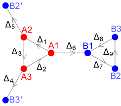
Figure 3: Real space pairing amplitudes, encoded in the $9$-dimensional vector, ${\bf\Delta}$, used in the mean-field analysis and linearized gap equations. The two triangular clusters in the unit cell are shown in red (A) and blue (B). For triplet superconductivity, the pairing amplitudes against the directions indicated by the arrows are minus the amplitudes along the arrow directions. In the singlet case arrows should be ignored since the pairing is non-directional.

IV.2 Mean-field OSP triplet RVB theory

With the considerations above we explore the possibility of triplet RVB superconductivity in our model (1). We perform a mean-field BCS decoupling of the magnetic terms in the hamiltonian. It is convenient to write the theory in terms of triplet bond operators [46, 26],

$$h_{\alpha i,\beta j}^{\dagger}={1\over\sqrt{2}}(c^{\dagger}_{\alpha i\uparrow}c^{\dagger}_{\beta j\downarrow}+c^{\dagger}_{\alpha i\downarrow}c^{\dagger}_{\beta j\uparrow}).$$ (13)

Whence, the XXZ exchange in model (1) can be expressed as

$$\sum_{\langle\alpha i,\beta j\rangle}(S^{x}_{\alpha i}S^{x}_{\beta j}+S^{y}_{\alpha i}S^{y}_{\beta j}-S^{z}_{\alpha i}S^{z}_{\beta j}+{n_{\alpha i}n_{\alpha j}\over 4})=\sum_{\langle\alpha i,\beta j\rangle}h_{\alpha i,\beta j}^{\dagger}h_{\alpha i,\beta j},$$ (14)

We consider a BCS decoupling of the hamiltonian described through the pairing amplitudes:

$$\Delta_{\alpha i,\beta j} = \langle h_{\alpha i,\beta j}\rangle.$$ (15)

The mean-field hamiltonian with the renormalization effects due to the no double occupancy constraint, is then,

$${\cal H}_{MF}={\cal H}_{t}+{\cal H}_{J}$$ (16)

where:

$${\cal H}_{t} = -{\tilde{t}}\sum_{{\bf k}\langle\alpha i,\alpha j\rangle,\sigma}\left(c^{\dagger}_{\alpha i\sigma}({\bf k})c_{\alpha j\sigma}({\bf k})+h.c.\right)-{\tilde{t}}^{\prime}\sum_{\begin{subarray}{c}{\bf k},\langle Ai,Bi\rangle,\sigma\end{subarray}}\left(e^{i{\bf k}\cdot{\bf\delta}_{Ai,Bi}}c^{\dagger}_{Ai\sigma}({\bf k})c_{Bi\sigma}({\bf k})+h.c.\right),$$

$${\cal H}_{J}= - {{\tilde{J}}\over\sqrt{2}}\sum_{{\bf k}\langle\alpha i,\alpha j\rangle}\left(\Delta_{\alpha i,\alpha j}c^{\dagger}_{\alpha i\uparrow}({\bf k})c^{\dagger}_{\alpha j\downarrow}(-{\bf k})-\Delta_{\alpha i,\alpha j}c^{\dagger}_{\alpha j\uparrow}({\bf k})c^{\dagger}_{\alpha i\downarrow}(-{\bf k})\right)+h.c.$$ (17)

$$- {{\tilde{J}}^{\prime}\over\sqrt{2}}\sum_{{\bf k}\langle Ai,Bi\rangle}\left(\Delta_{Ai,Bi}e^{i{\bf k}\cdot{\bf\delta}_{Ai,Bi}}c^{\dagger}_{Ai\uparrow}({\bf k})c^{\dagger}_{Bi\downarrow}(-{\bf k})-\Delta_{Ai,Bi}e^{-i{\bf k}\cdot{\bf\delta}_{Ai,Bi}}c^{\dagger}_{Bi\uparrow}({\bf k})c^{\dagger}_{Ai\downarrow}(-{\bf k})\right)+h.c.$$

$$+ {\tilde{J}}\sum_{\langle\alpha i,\alpha j\rangle}|\Delta_{\alpha i,\alpha j}|^{2}+{\tilde{J}}^{\prime}\sum_{\langle Ai,Bi\rangle}|\Delta_{Ai,Bi}|^{2}+\mu\sum_{\alpha{\bf k}\sigma}c^{\dagger}_{\alpha\sigma}({\bf k})c_{\alpha\sigma}({\bf k}),$$

where we have made the Gutzwiller approximation (GA), which yields renormalized parameters: ${\tilde{t}}/t={\tilde{t}}^{\prime}/t^{\prime}={2\delta/(1+\delta)}\equiv g_{t}$ and ${\tilde{J}}/J={\tilde{J}}^{\prime}/J^{\prime}={4/(1+\delta)^{2}}\equiv g_{J}$. The numbering of sites in two neighboring $A,B$ triangles together with the different pairing amplitudes entering the Gorkov decoupling are shown in Fig. 3.

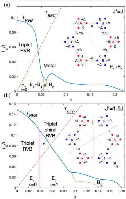
Figure 4: $T$ vs $\delta$ phase diagrams of the $t$-$J$ model (1) from triplet-RVB theory for (a) $J^{\prime}/J=1$ and (b) $J^{\prime}/J=1.5$. Superconductivity occurs when $T<T_{\text{BEC}}$ (red dashed line) and $T<T_{\text{RVB}}$ (blue line). While the transition at $T_{\text{RVB}}$ (blue solid line) is second order, the transitions between different superconducting orders can be first (green dotted lines) or second (green solid lines) order. A second order topological transition (pink solid line) separates E₁ ($\nu=0$) and E₁ ($\nu=1$) in (b). The insets in (a) and (b) illustrate the pairing patterns of the $p+f$ (E₁+B₁) and $f$ (B₂) solutions including their nodal lines in real space (black dashed lines). We have used $J=0.1t$ and $J^{\prime}/J=t^{\prime 2}/t^{2}$.

After diagonalization, the hamiltonian reads

$$H_{MF} = \sum_{m,{\bf k},\sigma}\omega_{m}({\bf k})\left(\gamma^{\dagger}_{m\sigma}({\bf k})\gamma_{m\sigma}({\bf k})-{1\over 2}\right)$$

$$+ {\tilde{J}}\sum_{\langle\alpha i,\alpha j\rangle}|\Delta_{\alpha i,\alpha j}|^{2}+{\tilde{J}}^{\prime}\sum_{\begin{subarray}{c}\langle Ai,Bi\rangle\end{subarray}}|\Delta_{Ai,Bi}|^{2}$$

where $\omega_{m}({\bf k})>0$ with $m=1,...,6$ are the positive Bogoliubov quasiparticle dispersions.

The free energy of the system is

$$\Phi = -{1\over\beta}\sum_{m,{\bf k},\sigma}\ln(1+e^{-\beta\omega_{m}({\bf k})})-\sum_{m,{\bf k}}\omega_{m}({\bf k})+6N_{s}\mu$$ (19)

$$+ {\tilde{J}}\sum_{\langle\alpha i,\alpha j\rangle}\left(|\Delta_{\alpha i,\alpha j}|^{2}\right)+{\tilde{J}}^{\prime}\sum_{\begin{subarray}{c}\langle Ai,Bi\rangle\end{subarray}}\left(|\Delta_{Ai,Bi}|^{2}\right)$$

From the minimization of the free energy we arrive at a set of self-consistent equations (SCEs):

$$\Delta_{\alpha i,\alpha j} = -{1\over{\tilde{J}}N_{s}}\sum_{m,{\bf k},\sigma}\left(f(\omega_{m}({\bf k}))-{1\over 2}\right)\left({\partial\omega_{m}({\bf k})\over\partial\Delta^{*}_{\alpha i,\alpha j}}\right),$$

$$\Delta_{Ai,Bi} = -{1\over{\tilde{J}}^{\prime}N_{s}}\sum_{m,{\bf k},\sigma}\left(f(\omega_{m}({\bf k}))-{1\over 2}\right)\left({\partial\omega_{m}({\bf k})\over\partial\Delta^{*}_{Ai,Bi}}\right),$$

$$\delta = -{1\over 6N_{s}}\sum_{m,{\bf k},\sigma}\left(f(\omega_{m}({\bf k}))-{1\over 2}\right)\left({\partial\omega_{m}({\bf k})\over\partial\mu}\right),$$

which we solve numerically.

IV.3 Phase diagrams and spinon dispersions

We now consider uniform metallic and superconducting solutions of the SCEs (LABEL:eq:sce). As in singlet RVB theory, there are two temperature scales: $T_{\text{RVB}}$ and $T_{\text{BEC}}$, which signify the onset of fermionic pairing and coherence respectively (the latter is corresponds to Bose-Einstein condensation in the slave boson reformulation of theory [52]).

tRVB theory allows us to characterize the superconducting states emerging in the $t$-$J$ model for different $J^{\prime}/J$ and $\delta$. The phase diagrams of the $J^{\prime}=J$ and $J^{\prime}=1.5J$ are shown in Fig. 4. The phase diagrams share similar qualitative features. At zero doping there is a ferromagnetic quantum spin liquid [37]. For $T<T_{\text{RVB}},T_{\text{BEC}}$ there is pairing and coherence, so we have triplet superconducting phases. For $T_{\text{RVB}}<T<T_{\text{BEC}}$ there is coherence but no pairing, and we have a conventional Fermi liquid. For $T_{\text{RVB}},T_{\text{BEC}}<T$ there is neither pairing nor coherence, so we have a strange metal. All of these phases are closely analogous to the phases in the same regimes of the singlet RVB theory [2].

However, for $T_{\text{BEC}}<T<T_{\text{RVB}}$, there is pairing but no coherence. In the singlet RVB theory this is interpreted as a spin gap or pseudogap [2]. In the tRVB theory we need to take care as we are dealing with triplet, rather than singlet, pairs. Furthermore, the strong SMOC assumed in the derivation of the XXZ model (Eq. (3)) implies that the ‘spins’ in our model are actually spin-orbit entangled pseudospins. Therefore, we expect a gap for longitudinal magnetic fields, but no gap for transverse magnetic fields in the tRVB pseudogap phase. This contrasts with the singlet-RVB state where the (pseudo)gap is apparent for any magnetic field direction. For the tRVB state for sufficiently large longitudinal fields (relative to the strength of the spin-orbit coupling) we expect, on general energetic grounds, a transition where the triplet order parameter rotates to be perpendicular to the field [53], this is analogous Fréedericksz transition in liquid crystals and ³He in slab geometries [54].

In both cases at the larger dopings at which weak coupling theory is relevant the most stable superconducting solution has $f$-wave (B₂) symmetry,

$${\bf\Delta}(\text{B}_{2})=[(1,1,1),(0,0,0),(-1,-1,-1)],$$ (21)

which is sketched in the inset of Fig. 4(b). As expected, given the scalar order parameter, this $f$-wave triplet superconducting solution displays three nodal lines in real space.

In the strong coupling regime, $\delta\rightarrow 0$, a $p+ip$ (E₁) superconducting phase is found to be the ground state for both exchange $J^{\prime}/J=1$ and $J^{\prime}/J=1.5$. This state displays a complex order parameter given by:

$${\bf\Delta}(\text{E}_{1})= [(1,0,-1),(0,0,0),(-1,0,1)]$$ (22)

$$+e^{i\alpha_{1}}[(1,-1,0),(0,0,0),(-1,1,0)]$$

$$-\Delta^{\prime}\big{(}e^{i\alpha_{2}}[(0,0,0),(2,-1,-1),(0,0,0)]$$

$$+\sqrt{3}e^{i\alpha_{1}}[(0,0,0),(0,1,-1),(0,0,0)]\big{)},$$

with lightly $\delta$-dependent phases around $\alpha_{1}=\pi/3$ and $\alpha_{2}=\pi/6$ (up to numerical accuracy) and the amplitude $\Delta^{\prime}$ strongly dependent on the doping. Clearly, this state breaks time reversal symmetry.

However, important differences between the two phase diagrams appear in the intermediate doping range. For $J^{\prime}=J$ the E₁ and B₂ pairing states are separated by two superconducting states obtained from the mixing of two different irreducible representations of Table 1. At $\delta>0.023$, a second order transition to a $p+f$ (E₁+B₁) symmetry superconducting state occurs, where

$${\bf\Delta}(\text{E}_{1}+\text{B}_{1})=[(1,0,-1),(-\alpha,\alpha^{\prime},-\alpha),(-1,0,1)],$$ (23)

has the lowest energy. The intertriangle amplitudes ratio $\alpha^{\prime}/\alpha$ has a doping dependence which is analyzed in Appendix C (see especially Fig. 15). By raising the doping above $\delta\sim 0.053$ a first order transition to a $p+f^{\prime}$ (E₁+B₂) pairing state occurs, which order parameter reads

$${\bf\Delta}(\text{E}_{1}+\text{B}_{2})=[(1,1,\eta),(-\xi,\xi,0),(-1,-1,\eta)],$$ (24)

with $0<\eta,\xi<1$. Then at $\delta=0.064$ the system transits to the pure f-wave (B₂) described above. These pairing states come from linear combinations of $p$ (E₁) and $f$ (either B₁ or B₂) superconducting solutions (see Table. 1).

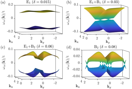
Figure 5: Mean-field BdG bands at a fixed temperature $T=0.01t$ for the different pairing symmetries at $J^{\prime}/J=1$. Only the occupied, $-\omega_{1}(\bf{k})$, and unoccupied, $\omega_{1}(\bf{k})$, bands closest to the Fermi level are shown for simplicity.

These ‘hybrid’ superconducting states are forbidden in the linearized gap equations (see discussion of $T_{c}$s in the following subsection), as every solution must transform according to a single representation of C_6v [55]. However, when the superconducting state lowers the symmetry of the system to ${\cal G}$, a subgroup of C_6v, then any harmonic transforming according to the same irreducible representation of ${\cal G}$ as the superconducting order parameter can mix without breaking additional symmetries and hence causing a phase transition (immediately) below $T_{c}$. A full mathematical discussion of this is given in Appendix C based on the the general framework [55]. For $p$-wave (E₁) solutions on the DHL the only other representations of C_6v that can mix are $f$-wave (B₁ and B₂). Thus, in $p+f^{(\prime)}$ states are common on the DHL as they often have lower energy than pure $p$-wave states.

For $J^{\prime}=1.5J$ the complex $p+ip$ solution (22) survives for much higher dopings relegating the B₂ state to a small doping region. The E₁ superconducting parameter increases rapidly as doping decreases ($||\bm{\Delta}(\text{E}_{1})||\gg 1$ for $\delta\rightarrow 0$). Furthermore, we find a second order transition at $\delta_{c}=0.039$ above which the $p+ip$ superconducting state becomes topologically non-trivial with a Chern number $\nu=1$. The $p+ip$ (E₁) topological superconductor, will be discussed in detail in Sec. V.

The superconducting order parameter in reciprocal space can be quite different to its real space counterpart as expected in a multiband system.[50] In Fig. 5 we show the doping dependence of the lowest energy BdG excitations for $J^{\prime}=J$. In marked contrast to one band systems, the nodal structure of the dispersions of the present multiband system (with many atoms per unit cell), is very different to the one in real space. For instance, the $f$-wave (B₂) solution of Fig. 5(d) displays only isolated nodal points in contrast to the three nodal lines occurring in real space. Similarly, the $p+f$ (E₁+B₁) state shown in 5(b) is characterized by two nodal points along $k_{y}=k_{x}$ in the BdG bands although the superconducting state has a single nodal line in real space (see inset of Fig. 4(a)). The $p+f$ (E₁+B₂) state is gapped over the entire Brillouin zone in contrast to the three nodal lines occurring in real space. Only in the $p+ip$ (E₁) superconducting phases the order parameter is found to be fully gapped consistently in real and reciprocal space as illustrated in Fig. 5(a) for $\delta=0.015$. At the critical lines of the Fig. 4 phase diagrams separating E₁ solutions with different topological properties nodal points occur.

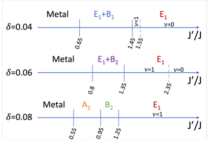
Figure 6: Dependence of superconducting states on dimerization/trimerization, $J^{\prime}/J$. The phase diagrams of model (1) at three different dopings: $\delta=0.04,0.06,0.08$ are shown at fixed $T=0.01$. We have used $J=0.1t$ and $J^{\prime}/J=t^{\prime 2}/t^{2}$.

Thus an overall trend emerges: at strong coupling, $\delta\rightarrow 0$, when the system is dominated by magnetic exchange the SC is characterized by either having isolated nodal points or being fully gapped. In contrast, the weak coupling solutions at large $\delta$ are dominated by the kinetic energy and the gap has nodal points in reciprocal space. Hence, gapless superconductivity is more common in the weak coupling regime than at strong coupling.

Hybrid and topological superconductivity are not peculiar to the specific $J^{\prime}/J$ explored in Fig. 4. The phase diagrams of Fig. 6 show that the hybrid E₁+B₁ and E₁+B₂ states occur at low $\delta\sim 0.04-0.06$ in an extend range of $J^{\prime}/J$, consistent with the analysis of Appendix C. At larger dopings, say $\delta=0.08$, pure A₂, B₂ and E₁ are favored, respectively, as $J^{\prime}/J$ increases consistent with the weak coupling analysis of Appendix A. On the other hand, topological $p+ip$ (E₁) superconductivity (with $\nu=1$) is favored in the dimerized regime, $J^{\prime}/J>1$, and increasing $\delta$, Fig. 6. As doping increases the topological transition to the trivial E₁ superconducting state ($\nu=0$) occurs deeper into the dimerized limit. Hence, hybrid and topological superconductivity are robust solutions of the SCE of model (1).

IV.4 Critical temperatures and superconducting pairing states

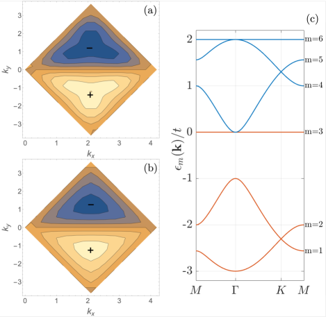
Figure 7: Triplet gap function projected onto the occupied bands closest to Fermi energy. The intraband gaps, $\Delta_{22}({\bf k})$ (a) and $\Delta_{33}({\bf k})$ (b) corresponding to the $f$-wave (B₂) solution for $\delta=0.09$ and $J^{\prime}=J$ are shown. Note the different scale of the pairing amplitude in the two figures: (a) -0.068-0.068; (b) -0.64-0.64. (c) Bare bands (eigenstates of $\mathcal{H}_{t}$, Eq. (17) for $\tilde{t}=t=\tilde{t}^{\prime}=t^{\prime}$) .

Additional understanding can be gained from a weak coupling microscopic analysis to obtain the $T_{c}$s of the different possible pairing solutions. The set of SCE (LABEL:eq:sce) can be linearized by expanding the quasiparticle energies around $T_{c}$. This yields

$$\omega_{m}({\bf k})=\epsilon_{m}({\bf k})+\sum_{n}{|\Delta_{mn}({\bf k})|^{2}\over\epsilon_{m}({\bf k})+\epsilon_{n}({\bf k})},$$ (25)

where the $\epsilon_{m}({\bf k})$ are the eigenvalues of the kinetic energy part of the mean-field part of the hamiltonian, ${\cal H}_{t}$, Eq. (17), with $m$ running from the lowest to highest energy band (shown in Fig. 7(c)). The gap functions projected onto the different bands, $\Delta_{mn}({\bf k})$, read:

$$\Delta_{mn}({\bf k})=\sum_{p}{\tilde{J}_{p}}\Omega^{p}_{mn}({\bf k})\Delta_{p},$$ (26)

where $m,n$ denote the different bands and $p=1,..,9$ with $\Delta_{p}$, the real space Cooper pairing amplitudes of Eq. (12), shown in Fig. 3, and ${\tilde{J}_{p}}={\tilde{J}}$ for $p=1,2,3$ and $p=7,8,9$ while ${\tilde{J}_{p}}={\tilde{J}^{\prime}}$ for $p=4,5,6$, and the $\Omega^{p}_{mn}({\bf k})$ are products of Bloch wavefunction coefficients defined in Eq. (A).

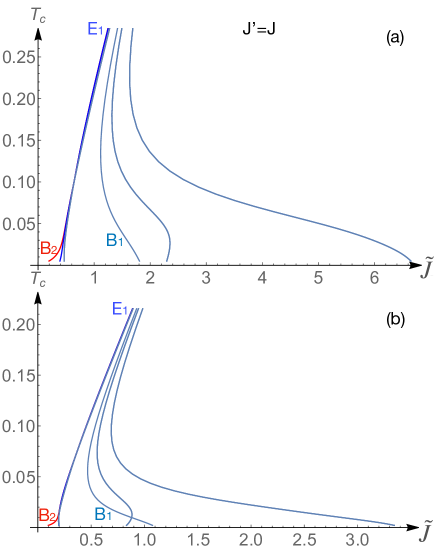
Figure 8: Dependence of the superconducting critical temperatures on the strength of the magnetic coupling, ${\tilde{J}}$ obtained from the linearized gap equations at $J^{\prime}=J$ for doping (a) $\delta=0.1$ and (b) $\delta=0.04$. The most favorable solution at a given ${\tilde{J}}$ occurs for the channel with the highest $T_{c}$. While the dominant superconducting solution at small coupling, ${\tilde{J}}\rightarrow 0$, is $f$-wave (B₂; red solid line), at large ${\tilde{J}}$, the doubly-degenerate $p$ wave (E₁; magenta solid line) solution is found. $t=1$ in these plots.

We can understand the differences between real and reciprocal space pairing by comparing the intra- and intra-band order parameters. The intraband gap functions, $\Delta_{mm}({\bf k})$, for $f$-wave (B₂) solutions for $J^{\prime}=J$ and $\delta=0.09$ with $m=2,3$, shown in Fig. 7, provide a typical example. The solution in ${\bf k}$-space projected onto the flat band at the Fermi energy, $m=3$, shows a $p_{y}$-wave structure (i.e., it is odd under $k_{y}\rightarrow-k_{y}$, but even under $k_{y}\rightarrow-k_{x}$) similar to the lowest energy BdG dispersion, Fig. 5(d). However, we also find large that the interband contributions, $|\Delta_{m3}({\bf k})|\lesssim 0.22$ for $m\neq 3$, can be quite large compared to the intraband contribution $|\Delta_{33}({\bf k})|\sim 0.64$. This is important for understand why the real space and reciprocal space pictures are so different. Even more remarkably, for $p+f$ (E₁+B₁) superconductivity, $\Delta_{33}({\bf k})=0$, which means that, the interband contributions $|\Delta_{m3}({\bf k})|$ are solely responsible the gap in the BdG spectrum, Fig. 5(b).

The set of linearized gap equations at T_c obtained by introducing the approximate BdG dispersions, $\omega_{m}({\bf k})$ in Eq. (LABEL:eq:sce), read

$$\Gamma{\bf{\tilde{\Delta}}}={1\over{\tilde{J}}}{\bf{\tilde{\Delta}}},$$ (27)

where ${\bf{\tilde{\Delta}}}=({\tilde{J}}\Delta_{A},{\tilde{J}}^{\prime}\Delta_{X},{\tilde{J}}\Delta_{B})$. Solving for the eigenvalues of (27), $1/{\tilde{J}}^{\lambda}$, we can conveniently obtain the dependence of T_c on ${\tilde{J}}$ in the different pairing channels: $\lambda$, described by the eigenvectors ${\tilde{\Delta}}_{\lambda}$ (see Appendix A for details). These eigenvectors can be classified according to the character table 1 as it should since the matrix $\Gamma$ respects the C_6v point group symmetry of the lattice.

The elements of the $9\times 9$ matrix $\Gamma$ are

$$\Gamma_{pq} = {1\over 2N_{s}}{\tilde{J}_{p}\over\tilde{J}}\sum_{m,n,{\bf k}}\tanh({\epsilon_{m}({\bf k})\over 2k_{B}T}){1\over\epsilon_{m}({\bf k})+\epsilon_{n}({\bf k})}$$ (28)

$$\times\left(\Omega^{*p}_{mn}({\bf k})\Omega^{q}_{mn}({\bf k})+\Omega^{p}_{mn}({\bf k})\Omega^{*q}_{mn}({\bf k})\right).$$

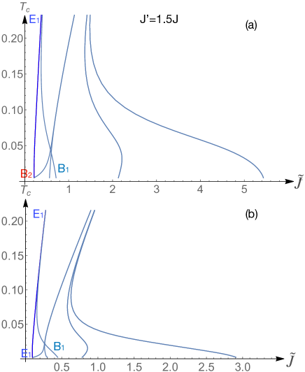
Figure 9: Dependence of the superconducting critical temperatures on ${\tilde{J}}$ obtained from the linearized gap equations at $J^{\prime}=1.5J$ for doping (a) $\delta=0.1$ and (b) $\delta=0.04$. While the dominant superconducting solution at weak coupling, ${\tilde{J}}\rightarrow 0$, the $p$-wave (E₁) and $f$-wave (B₂) solutions are degenerate within the accuracy of our calculations, for strong coupling the doubly-degenerate $p$-wave (E₁; magenta solid line) state has the highest $T_{c}$. $t=1$ in these plots.

We can gain insight into the phase diagrams of Fig. 4 obtained from the full SCE by analyzing the dependence of $T_{c}$ on the strength of the coupling, ${\tilde{J}}$, as obtained from the linearized gap equation (27). The $T_{c}$s obtained from (27) for $J^{\prime}=J$ and $J^{\prime}=1.5J$ are shown in Figs. 8 and 9 respectively. From these plots one can obtain useful information about the dominant pairing channel which is given by the one with the largest $T_{c}$ for a given ${\tilde{J}}$.

In the full phase diagrams of Fig. 4 as $\delta\rightarrow 0$ the effective coupling increases, ${\tilde{J}}/{\tilde{t}}\propto g_{J}/g_{t}\propto 1/\delta$ due to the effect of the GA projection. We consistently find that the $f$-wave (B₂) solution arises for large doping $\delta\sim 0.1-0.2$ in the solution of the SCEs indeed has the highest $T_{c}$ in the linearized equations as ${\tilde{J}}\rightarrow 0$, Figs. 8(a) and 9(a). As ${\tilde{J}}$ increases the $E_{1}$ has the highest $T_{c}$. However, the $T_{c}$’s of other solutions become very similar to the $T_{c}$ of the E₁ solution. This means that several superconducting solutions are numerically indistinguishable. The E₁, A₂, and B₂ solutions have nearly identical $T_{c}$s and the $T_{c}$ of the B₁ solution is becomes close to these as ${\tilde{J}}$ increases. This is consistent with the full non-linear SCE which while for $J^{\prime}=1.5J$ give a pure E₁ solution, for $J^{\prime}=J$ a E₁+B₁ combination eventually wins. The SCE also show that for $J^{\prime}=1.5J$ a complex combination of two E₁ is energetically favorable.

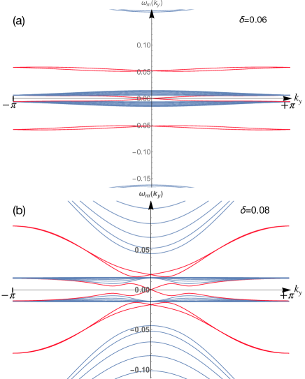
Figure 10: Topological edge states in the TSC (E₁) phase. The BdG band structure of a superconducting ribbon with zig-zag edges along the $y$-direction is shown for $J^{\prime}=1.5J$ and $\delta=0.06$ (top) and $\delta=0.08$ (bottom). The gapped BdG bands (blue) are traversed by surface edge states (red) crossing at $k_{y}=0$. Edge states are identified by direct comparison with the spectrum of the extended system. Note that as $t=1$ in these plots, the Majorana modes are extemely localized (i.e., the Majorana bands are extremely flat).

More details on the analysis of the $T_{c}$s are provided in Appendix A.

The ED pairing correlations at $\delta=0$ (see Appendix D) show that while the E₁ and B₁ solutions are dominant for $J^{\prime}/J>1/\sqrt{2}$, the A₂ and B₂ are favorable for $J^{\prime}/J<1/\sqrt{2}$. These limits are in good agreement with the present weak coupling analysis, considering the small six-site cluster analysed with ED.

V Topological superconductivity

Unambiguous signatures of non-trivial topology are found in both the presence of topological edge states and a non-zero topological bulk invariant, as guaranteed by the bulk-boundary correspondence. In the case of time reversal symmetry breaking superconductors the topological invariant is the Chern number $\nu$ which we evaluated as described in Appendix E. We find that the $p+ip$ (E₁) TSC phase has a Chern number, $\nu=1$, while the other phases discussed are non-topological, $\nu=0$.

From the Chern number calculation we conclude that the $p+ip$ (E₁) TSC has a single Majorana edge mode circulating around the edge of the sample. We obtain the edge states of a ribbon in the zig-zag geometry cut along the $y$-direction assuming the lattice orientation shown in Fig. 1. The ribbon is assumed to be in a superconducting state with pairing amplitudes given by the bulk solution, i.e., we do not perform a fully self-consistent calculation of the ribbon. We plot the projected BdG bands along the $k_{y}$ edge of a ribbon in the $p+ip$ (E₁) TSC state in Fig. 10. As well as the bulk bands, two edge states with opposite slopes (velocities) cross at $k_{y}=0$ inside the gap around zero energy. These correspond to the chiral edge state circulating in opposite directions on the two edges of the ribbon as expected for $\nu=1$. In contrast, no topological edge states are found in ribbons in the $f$-wave (B₂) and $p+f$ (E₁+B₁) superconducting phases as expected for $\nu=0$. Interestingly, the Majorana edge modes associated with the $p+ip$ (E₁) TSC are almost localized since it emerges within a small gap in nearly flat bands.

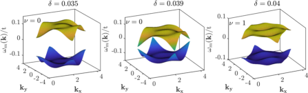
Figure 11: Dependence of the BdG bands, $\pm\omega_{1}({\bf k})$ on doping, $\delta$, across the low doping topological transition for $J^{\prime}/J=1.5$. At $T=0.01$ as $\delta$ increases from $\delta=0$ a topological gap with $\nu=1$ opens around $\delta_{c}\sim 0.385$ signalling the TSC(E₁) phase of Fig. 4.

A topological transition from the trivial $p+ip$ (E₁) superconductor to the topological $p+ip$ (E₁) superconductor occurs at $\delta_{c}\sim 0.039$ in the phase diagram 4 for $J^{\prime}=1.5J$. The smooth closing and reopening of the superconducting gap (see Fig. 11) is accompanied by the Chern number jump, $\Delta\nu=1$, which indicates a second order topological transition at $\delta_{c}$. At a larger $\delta$ ($\delta\approx 0.14$ at $T=0.01t$), a first order transition from the $p+ip$ (E₁) TSC to the non-topological $f$-wave (B₂) phase occurs. This contrasts with the doped Kitaev model[56] in which only first order transitions between superconducting states occur. At temperatures above the condensation temperature, $T>T_{\text{BEC}}$, the second order transition at $\delta_{c}$ becomes a transition from a tRVB to a chiral tRVB quantum spin liquid (see Fig. 4).

VI Conclusions

In this work we have found unconventional triplet superconductivity in an easy-axis XXZ ferromagnetic $t$-$J$ model on the DHL. The underlying mechanism is attributed to the preexistence of a tRVB spin liquid in the Mott phase which is suggested by numerical exact diagonalization calculations. The symmetry of the superconducting order parameter depends sensitively on both $J^{\prime}/J$ and doping. This is a direct consequence of the flat band, which favors many superconducting channels.

At small $\delta$ ferromagnetic interactions dominate leading to exotic phases including topological superconductivity. However, at large $\delta$ superconductivity is mainly weak coupling, and strongly influenced by band structure effects. A similar situation including topological superconductivity was predicted for hole doped Kitaev spin liquids with ferromagnetic exchange interactions.[56]

Generically, lines of first order transitions separate different superconducting phases. The important exception to this is the transition from topologically trivial $p+ip$ (E₁) superconductivity to topological $p+ip$ (E₁) superconductivity with Chern number, $\nu=1$. This transition is continuous, which is possible as both states transform according to the same irreducible representation of $C_{6v}$. This occurs in a two-dimensional representation is, perhaps, unsurprising in retrospect, as two-dimensional representations lead quite naturally to broken time reversal symmetry [57].

Topological superconductivity occurs in a broad doping range of the phase diagram being favored at large $J^{\prime}/J$. Critical temperatures of $T_{c}\sim 0.8J$ are reached at optimal hole doping, $\delta\sim 0.06$ for $J^{\prime}=1.5J$. The corresponding Majorana edge modes obtained at the lowest dopings are almost localized in two flat bands close to the Fermi level. This suggests that topological superconductivity in flat band materials could be useful for decoherence free topological quantum computing schemes based on localized Majorana modes.

We have shown that the nodal structures of the superconducting gap appear very different in real space and reciprocal space. This results from the need to transform from a real-space multi-site basis to a reciprocal space multi-band basis. There is nothing special about the DHL lattice in this regard. Therefore, we expect this to be observed in any superconductor where multiple (atomic [50] or molecular) orbitals at distinct sites contribute significant density of states near the Fermi energy.

It is also interesting that we observed $p+f$ superconductivity with only a single superconducting transition even though $p$-wave and $f$-wave superconductors belong to different representations of C_6v – the point group describing the DHL, E₁ and B₁ or B₂ respectively. This occurs because the dominant $p$ wave superconducting state lowers the symmetry of the system, such that the $p$-wave and $f$-wave belong to the same irreducible representation, i.e., they become overtones, and arbitrary admixtures are allowed without breaking additional symmetries. That this is possible has long been understood [55, 15], however there are still relatively few detailed calculations where this is observed.

A crucial ingredient of our model is the easy-plane ferromagnetic interaction which can arise in spin orbit Mott insulators. Although candidate materials such as Mo₃S₇(dmit)₃, (EDT-TTF-CONH₂)₆[Re₆Se₈(CN)₆], and Rb₃TT$\cdot$2H₂O host strong correlations on a DHL antiferromagnetic interactions are dominant. Increasing SMOC in these candidate materials, for example by synthesizing the Se analogue of Mo₃S₇(dmit)₃ or finding other spin orbit Mott insulators on DHLs are routes for realizing triplet superconductivity under hole doping. Hole doping has been achieved in certain organics[58] but only at a specific doping fixed by the chemistry of the constituents. Clearly, experimental progress in hole doping techniques are required to enlarge hole doping ranges in organic and organometallic materials and test our prediction of triplet topological superconductivity in the DHL.

Appendix A Superconducting critical temperatures and pairing symmetries

We now analyze the pairing symmetries and $T_{c}$s based on the weak coupling analysis of Section IV.4 of the main text.

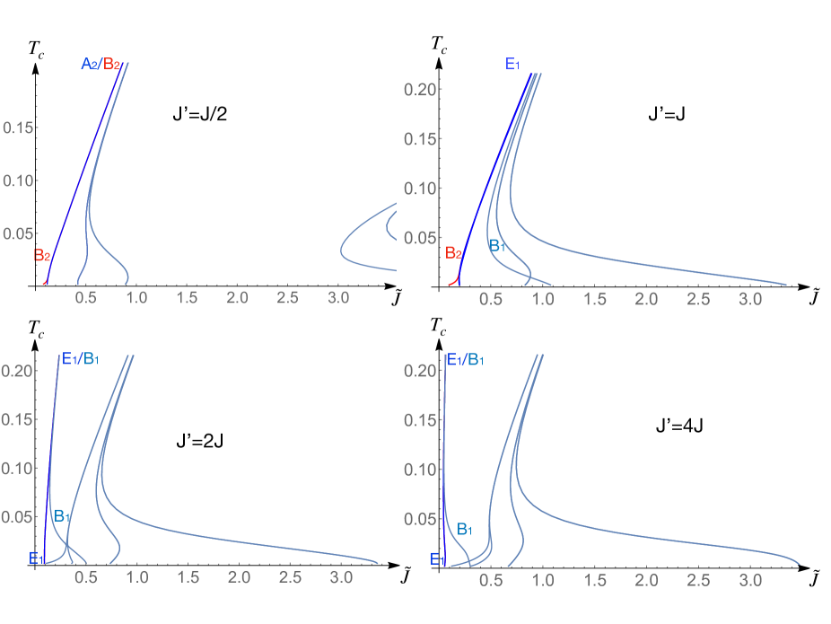
Figure 12: Dependence of the critical temperatures in different pairing channels on the strength of the magnetic coupling, ${\tilde{J}}$, for different ratios $J^{\prime}/J$ at $\delta=0.04$ obtained from the linearized gap equations. The most favorable solution at a given ${\tilde{J}}$ occurs for the channel with the highest $T_{c}$.

The matrix elements, $\Omega^{p}_{mn}({\bf k})$ in Eq. (28) read:

$$\Omega^{1}_{mn}({\bf k}) = C_{A1}^{*}(\epsilon_{m})C_{A2}(\epsilon_{n})+C_{A2}^{*}(\epsilon_{m})C_{A1}(\epsilon_{n})$$

$$\Omega^{2}_{mn}({\bf k}) = C_{A1}^{*}(\epsilon_{m})C_{A3}(\epsilon_{n})+C_{A3}^{*}(\epsilon_{m})C_{A1}(\epsilon_{n})$$

$$\Omega^{3}_{mn}({\bf k}) = C_{A2}^{*}(\epsilon_{m})C_{A3}(\epsilon_{n})+C_{A3}^{*}(\epsilon_{m})C_{A2}(\epsilon_{n})$$

$$\Omega^{4}_{mn}({\bf k}) = C_{A1}^{*}(\epsilon_{m})C_{B1}(\epsilon_{n})e^{i{\bf k}{\delta}_{1}}+C_{B1}^{*}(\epsilon_{m})C_{A1}(\epsilon_{n})e^{-i{\bf k}{\delta}_{1}}$$

$$\Omega^{5}_{mn}({\bf k}) = C_{A2}^{*}(\epsilon_{m})C_{B2}(\epsilon_{n})e^{i{\bf k}{\delta}_{2}}+C_{B2}^{*}(\epsilon_{m})C_{A2}(\epsilon_{n})e^{-i{\bf k}{\delta}_{2}}$$

$$\Omega^{6}_{mn}({\bf k}) = C_{A3}^{*}(\epsilon_{m})C_{B3}(\epsilon_{n})e^{i{\bf k}{\delta}_{3}}+C_{B3}^{*}(\epsilon_{m})C_{A3}(\epsilon_{n})e^{-i{\bf k}{\delta}_{3}}$$

$$\Omega^{7}_{mn}({\bf k}) = C_{B1}^{*}(\epsilon_{m})C_{B2}(\epsilon_{n})+C_{B2}^{*}(\epsilon_{m})C_{B1}(\epsilon_{n})$$

$$\Omega^{8}_{mn}({\bf k}) = C_{B1}^{*}(\epsilon_{m})C_{B3}(\epsilon_{n})+C_{B3}^{*}(\epsilon_{m})C_{B1}(\epsilon_{n})$$

$$\Omega^{9}_{mn}({\bf k}) = C_{B2}^{*}(\epsilon_{m})C_{B3}(\epsilon_{n})+C_{B3}^{*}(\epsilon_{m})C_{B2}(\epsilon_{n}),$$

where the $C_{i}(\epsilon_{m})$ are the Bloch wave coefficients of the $m$-band:

$$|\Psi_{m}({\bf k})\rangle={1\over\sqrt{N_{c}}}\sum_{\alpha,i}C_{\alpha i}(\epsilon_{m})\sum_{n}e^{i{\bf k}\cdot({\bf R}_{n}+{\bf d}_{\alpha i})}|\phi_{n\alpha i}\rangle,$$ (29)

where $|\phi_{n\alpha i}\rangle=|\phi({\bf r}-{\bf R}_{n}-d_{\alpha i})\rangle$. The symmetries of the pairing amplitudes are determined by these coefficients which carry the information of the lattice symmetries. From the eigenvalues of $\Gamma$, ${1\over{\tilde{J}}_{\lambda}}$, we obtain the Cooper pair formation energy, ${\tilde{J}}_{\lambda}$, in each channel pairing $\lambda$. The smaller the ${\tilde{J}}_{\lambda}$, the easier it is to form Cooper pairs in the corresponding channel. Hence, we can determine the dominant pairing channels allowed by symmetry given in Table 1.

We illustrate in detail the $J^{\prime}=J$ case which is amenable to analytical analysis. The structure of the $\Gamma$ matrix in Eq. (28) is:

$$\Gamma=\begin{pmatrix}A_{3\times 3}&B_{3\times 3}&C_{3\times 3}\\ B^{\intercal}_{3\times 3}&D_{3\times 3}&-B^{\intercal}_{3\times 3}\\ C_{3\times 3}&-B_{3\times 3}&A_{3\times 3}.\\ \end{pmatrix}$$

where:

$$A_{3\times 3}=\left(\begin{array}[]{ccc}a_{1}&a_{2}&a_{2}\\ a_{2}&a_{1}&a_{2}\\ a_{2}&a_{2}&a_{1}\\ \end{array}\right),$$ (33)

$$B_{3\times 3}=\left(\begin{array}[]{ccc}0&b_{1}&-b_{1}\\ -b_{1}&0&b_{1}\\ b_{1}&-b_{1}&0\\ \end{array}\right),$$ (37)

$$C_{3\times 3}=\left(\begin{array}[]{ccc}c_{1}&c_{2}&c_{2}\\ c_{2}&c_{1}&c_{2}\\ c_{2}&c_{2}&c_{1}\\ \end{array}\right),$$ (41)

and

$$D_{3\times 3}=\left(\begin{array}[]{ccc}d_{1}&d_{2}&d_{2}\\ d_{2}&d_{1}&d_{2}\\ d_{2}&d_{2}&d_{1}\\ \end{array}\right).$$ (45)

From the common eigenvectors: $\phi_{sym}$, of the $A,B,C,D$ matrices and their corresponding eigenvalues: $\tilde{a}_{sym},\tilde{b}_{sym},\tilde{c}_{sym}$ and $\tilde{d}_{sym}$ we can find solutions analytically. Introducing: $[\Delta_{\lambda}]^{\intercal}=(\phi_{sym},(0,0,0),\pm\phi_{sym})$ in Eq. (27) leads to the A₂ and B₂ solutions:

$$[\Delta(\text{A}_{2})]^{\intercal} \propto[(1,1,1),(0,0,0),(1,1,1)]$$

$$[\Delta(\text{B}_{2})]^{\intercal} \propto[(1,1,1),(0,0,0),(-1,-1,-1)]$$ (46)

with corresponding eigenvalues:

$${1\over{\tilde{J}}_{\text{A}_{2}}} =\tilde{a}_{sym}+\tilde{c}_{sym}=a_{1}+2a_{2}+(c_{1}+2c_{2}),$$

$${1\over{\tilde{J}}_{\text{B}_{2}}} =\tilde{a}_{sym}-\tilde{c}_{sym}=a_{1}+2a_{2}-(c_{1}+2c_{2}).$$ (47)

There are also two degenerate solutions of the E₂ type:

$$[\Delta(\text{E}_{2})]^{\intercal} \propto[(-1,0,1),(0,0,0),(-1,0,1)]$$

$$[\Delta(\text{E}_{2})]^{\intercal} \propto[(1,-1,0),(0,0,0),(1,-1,0)]$$ (48)

with the common eigenvalue:

$${1\over{\tilde{J}}_{\text{E}_{2}}}=a_{1}-a_{2}+c_{1}-c_{2}.$$ (49)

Finally, we find the B₁ solution:

$$[\Delta(\text{B}_{1})]^{\intercal}\propto[(0,0,0),(1,1,1),(0,0,0)],$$ (50)

with eigenvalue

$${1\over{\tilde{J}}_{\text{B}_{1}}}=d_{1}+2d_{2}.$$ (51)

So we have found five solutions of the type $[\Delta_{\lambda}]^{\intercal}=(\phi_{sym},(0,0,0),\pm\phi_{sym})$. There are four more solutions of the E₁ type:

$$[\Delta(\text{E}_{1}^{-})]^{\intercal} \propto((1,0,-1),(\beta,-2\beta,\beta),(-1,0,1))$$

$$[\Delta(\text{E}_{1}^{-})]^{\intercal} \propto((1,-1,0),(-\beta,-\beta,2\beta),(-1,1,0))$$

$$[\Delta(\text{E}_{1}^{+})]^{\intercal} \propto((1,0,-1),(-\alpha,2\alpha,-\alpha),(-1,0,1))$$

$$[\Delta(\text{E}_{1}^{+})]^{\intercal} \propto((1,-1,0),(\alpha,\alpha,-2\alpha),(1,-1,0))$$

where $\alpha\neq\beta$ in general. The above four states have corresponding eigenvalues:

$${1\over{\tilde{J}}_{\text{E}_{1}^{-}}} ={1\over 2}\left(a_{1}-a_{2}-c_{1}+c_{2}+d_{1}-d_{2}-\sqrt{(a_{1}-a_{2}-c_{1}+c_{2}+d_{1}-d_{2})^{2}+24b_{1}^{2}-4(a_{1}-a_{2}-c_{1}+c_{2})(d_{1}-d_{2})}\right)$$

$${1\over{\tilde{J}}_{\text{E}_{1}^{+}}} ={1\over 2}\left(a_{1}-a_{2}-c_{1}+c_{2}+d_{1}-d_{2}+\sqrt{(a_{1}-a_{2}-c_{1}+c_{2}+d_{1}-d_{2})^{2}+24b_{1}^{2}-4(a_{1}-a_{2}-c_{1}+c_{2})(d_{1}-d_{2})}\right)$$

In Fig. 12 we show the dependence of $T_{c}$ on the coupling strength for different anisotropies, $J^{\prime}/J=0.5,1,2$, and 4. We first discuss the results at weak coupling, ${\tilde{J}}\rightarrow 0$, which would correspond to large $\delta$ regime of Fig. 4 due to the GA projection. The $T_{c}$ of the B₂ solution (red solid line) is the highest for small ${\tilde{J}}$ when $J^{\prime},J=0.5,1$ or 1.5 (the weak coupling results for $J^{\prime}=1.5J$ and shown in Fig. 9). However, for $J^{\prime}=2J$, the E₁ solution becomes more stable than the B₂ as ${\tilde{J}}\rightarrow 0$. These results indicate that the B₂ solution is stable in a broad range of $J^{\prime}/J$ consistent with the full phase diagrams of Fig. 4.

On the other hand, as ${\tilde{J}}$ increases, other solutions become favoured. For $J^{\prime}=J/2$ the $T_{c}$s of the B₂ and the A₂ merge so that both solutions are favorable, for $J^{\prime}=J$ the E₁ is singled out having the highest $T_{c}$ among all solutions. We also note how the $T_{c}$ of the B₁ becomes the next most highest. In fact, for $J^{\prime}/J=2,4$, the $T_{c}$ of the B₁ converges to the $T_{c}$ of the E₁ within the ranges of the plot. This analysis is consistent with the E₁ and E₁+B₁ solutions found at small doping, $\delta$ in the phase diagrams of Fig. 4 and the competition between these solutions as $J^{\prime}/J$ is varied shown in the phase diagrams of Fig. 6.

Appendix B Exact diagonalization analysis

Here we give some details on the exact diagonalization calculations of model (1) at half-filling on small clusters. The ground state wavefunction and energy is compared with the $|\text{nn-tRVB}\rangle$ [Eq. (LABEL:eq:tRVB)]. On the six-site cluster we have 20 possible spin configurations:

$$|1\rangle = c^{\dagger}_{1\uparrow}c^{\dagger}_{2\uparrow}c^{\dagger}_{3\uparrow}c^{\dagger}_{4\downarrow}c^{\dagger}_{5\downarrow}c^{\dagger}_{6\downarrow}|0\rangle$$

$$|2\rangle = c^{\dagger}_{1\uparrow}c^{\dagger}_{2\uparrow}c^{\dagger}_{3\downarrow}c^{\dagger}_{4\uparrow}c^{\dagger}_{5\downarrow}c^{\dagger}_{6\downarrow}|0\rangle$$

$$|3\rangle = c^{\dagger}_{1\uparrow}c^{\dagger}_{2\uparrow}c^{\dagger}_{3\downarrow}c^{\dagger}_{4\downarrow}c^{\dagger}_{5\uparrow}c^{\dagger}_{6\downarrow}|0\rangle$$

$$|4\rangle = c^{\dagger}_{1\uparrow}c^{\dagger}_{2\uparrow}c^{\dagger}_{3\downarrow}c^{\dagger}_{4\downarrow}c^{\dagger}_{5\downarrow}c^{\dagger}_{6\uparrow}|0\rangle$$

$$|5\rangle = c^{\dagger}_{1\uparrow}c^{\dagger}_{2\downarrow}c^{\dagger}_{3\uparrow}c^{\dagger}_{4\uparrow}c^{\dagger}_{5\downarrow}c^{\dagger}_{6\downarrow}|0\rangle$$

$$|6\rangle = c^{\dagger}_{1\uparrow}c^{\dagger}_{2\downarrow}c^{\dagger}_{3\uparrow}c^{\dagger}_{4\downarrow}c^{\dagger}_{5\uparrow}c^{\dagger}_{6\downarrow}|0\rangle$$

$$|7\rangle = c^{\dagger}_{1\uparrow}c^{\dagger}_{2\downarrow}c^{\dagger}_{3\uparrow}c^{\dagger}_{4\downarrow}c^{\dagger}_{5\downarrow}c^{\dagger}_{6\uparrow}|0\rangle$$

$$|8\rangle = c^{\dagger}_{1\uparrow}c^{\dagger}_{2\downarrow}c^{\dagger}_{3\downarrow}c^{\dagger}_{4\uparrow}c^{\dagger}_{5\uparrow}c^{\dagger}_{6\downarrow}|0\rangle$$

$$|9\rangle = c^{\dagger}_{1\uparrow}c^{\dagger}_{2\downarrow}c^{\dagger}_{3\downarrow}c^{\dagger}_{4\uparrow}c^{\dagger}_{5\downarrow}c^{\dagger}_{6\uparrow}|0\rangle$$

$$|10\rangle = c^{\dagger}_{1\uparrow}c^{\dagger}_{2\downarrow}c^{\dagger}_{3\downarrow}c^{\dagger}_{4\downarrow}c^{\dagger}_{5\uparrow}c^{\dagger}_{6\uparrow}|0\rangle$$

$$|11\rangle = c^{\dagger}_{1\downarrow}c^{\dagger}_{2\uparrow}c^{\dagger}_{3\uparrow}c^{\dagger}_{4\uparrow}c^{\dagger}_{5\downarrow}c^{\dagger}_{6\downarrow}|0\rangle$$

$$|12\rangle = c^{\dagger}_{1\downarrow}c^{\dagger}_{2\uparrow}c^{\dagger}_{3\uparrow}c^{\dagger}_{4\downarrow}c^{\dagger}_{5\uparrow}c^{\dagger}_{6\downarrow}|0\rangle$$

$$|13\rangle = c^{\dagger}_{1\downarrow}c^{\dagger}_{2\uparrow}c^{\dagger}_{3\uparrow}c^{\dagger}_{4\downarrow}c^{\dagger}_{5\downarrow}c^{\dagger}_{6\uparrow}|0\rangle$$

$$|14\rangle = c^{\dagger}_{1\downarrow}c^{\dagger}_{2\uparrow}c^{\dagger}_{3\downarrow}c^{\dagger}_{4\uparrow}c^{\dagger}_{5\uparrow}c^{\dagger}_{6\downarrow}|0\rangle$$

$$|15\rangle = c^{\dagger}_{1\downarrow}c^{\dagger}_{2\uparrow}c^{\dagger}_{3\downarrow}c^{\dagger}_{4\uparrow}c^{\dagger}_{5\downarrow}c^{\dagger}_{6\uparrow}|0\rangle$$

$$|16\rangle = c^{\dagger}_{1\downarrow}c^{\dagger}_{2\uparrow}c^{\dagger}_{3\downarrow}c^{\dagger}_{4\downarrow}c^{\dagger}_{5\uparrow}c^{\dagger}_{6\uparrow}|0\rangle$$

$$|17\rangle = c^{\dagger}_{1\downarrow}c^{\dagger}_{2\downarrow}c^{\dagger}_{3\uparrow}c^{\dagger}_{4\uparrow}c^{\dagger}_{5\uparrow}c^{\dagger}_{6\downarrow}|0\rangle$$

$$|18\rangle = c^{\dagger}_{1\downarrow}c^{\dagger}_{2\downarrow}c^{\dagger}_{3\uparrow}c^{\dagger}_{4\uparrow}c^{\dagger}_{5\downarrow}c^{\dagger}_{6\uparrow}|0\rangle$$

$$|19\rangle = c^{\dagger}_{1\downarrow}c^{\dagger}_{2\downarrow}c^{\dagger}_{3\uparrow}c^{\dagger}_{4\downarrow}c^{\dagger}_{5\uparrow}c^{\dagger}_{6\uparrow}|0\rangle$$

$$|20\rangle = c^{\dagger}_{1\downarrow}c^{\dagger}_{2\downarrow}c^{\dagger}_{3\downarrow}c^{\dagger}_{4\uparrow}c^{\dagger}_{5\uparrow}c^{\dagger}_{6\uparrow}|0\rangle.$$ (52)

where $\ket{0}$ is the vacuum state. The ground state of the easy-plane ferromagnetic model is indeed the expected triplet $S=1,S_{z}=0$ which is described as:

$$|\Psi_{0}\rangle=\sum_{n}a_{n}|n\rangle.$$ (53)

where the coefficients are: $A=A_{17}=A_{22}=A_{15}=A_{11}=A_{36}=A_{4}=0.3165$; $B=A_{19}=A_{18}=A_{16}=A_{14}=A_{13}=A_{12}=A_{9}=A_{8}=A_{7}=A_{5}=A_{3}=A_{2}=0.17667$; and $C=A_{1}=A_{20}=0.1106$. The exact energy of the anisotropic FM model with $J^{\prime}=J$ is $\epsilon_{0}(\text{exact})=-3.541287J$. The exact wavefunction compares well with the normalized $|\text{nn-tRVB}\rangle$ state whose non-zero coefficients are $A=0.3638$ and $B=C=0.1212$ giving the overlap $|\langle\text{tRVB}|\Psi_{0}\rangle|=0.9747$ quoted in Sec. III.1.

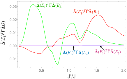
Figure 13: Dependence on $J^{\prime}/J$ of the hybridization between the gap functions associated with the irreducible representations of C_6v on the DHL. The matrix elements of Eq. (55) with $\lambda=\text{E}_{1}$ and $\lambda^{\prime}=\text{B}_{1},\text{B}_{2},\text{A}_{2}$ and E₂ are plotted for $\delta=0.04$ and $T/t=0.01<T_{c}$. Note that only the E₁-B₁ and E₁-B₂ matrix elements are non-zero indicating the possibility of hybrid $p+f$ (E₁+B₁ and E₁+B₂) superconducting states, and ruling out $p+i$ (E₁+A₂) or $p+d$ (E₁+E₂) superconductivity.

Appendix C Hybrid superconducting states

As well as the pure pairing states allowed by crystal symmetry, the SCE also yield solutions involving more than one irreducible representations of the C_6v group. As shown Fig. 4, two $p+f$ (E₁+B₁ and E₁+B₂) states occur for $J^{\prime}=J$. Naively one would expect that only solutions belonging to the same irreducible representation of the character table 1 are allowed. However, this is only true for the linearized gap equations (26) at $T_{c}$ since, in that case, the irreducible representations are eigenfunctions of the $\Gamma$-matrix. This is because Eq. (26) obeys the full C_6v symmetry of the DHL lattice (since it only depends on the bare band dispersions of the DHL).

However, for $T<T_{c}$, i.e., once superconductivity has set in, the C_6v symmetry of the system is spontaneously lowered to a new group, ${\cal G}$, which is a subgroup of C_6v. Thus, superconducting orders associated with different irreducible representations of C_6v may mix, if and only if the are in the same irreducible representation of ${\cal G}$. In order to explore possible mixing of superconducting orders we follow [55] and compute the matrix elements connecting different irreducible representations via a modified $\Gamma$ matrix that explicitly contains the symmetry breaking due to the superconducting order,

$${\tilde{\Gamma}}_{pq} = {1\over 2N_{s}}{\tilde{J}_{p}\over\tilde{J}}\sum_{m,n,{\bf k}}\tanh({\omega_{m}({\bf k})\over 2k_{B}T}){1\over\epsilon_{m}({\bf k})+\epsilon_{n}({\bf k})}$$ (54)

$$\times\left(\Omega^{*p}_{mn}({\bf k})\Omega^{q}_{mn}({\bf k})+\Omega^{p}_{mn}({\bf k})\Omega^{*q}_{mn}({\bf k})\right),$$

where $\omega_{m}({\bf k})$ is given by the second order expression (25) with $\Delta_{mn}({\bf k})$ evaluated with the real space gap function, $\Delta(\gamma)$. Note that this expression is appropriate to describe superconducting order below $T_{c}$ since $\omega_{m}({\bf k})$ enters this expression in the place of $\epsilon_{m}$ in the expression for $\Gamma$ (Eq. (28)).

Taking $\Delta(\lambda)$ as the dominant gap function, i.e., the one with the highest $T_{c}$, we evaluate matrix elements with the rest of gap functions of the character table 1. These matrix elements read:

$${\tilde{\bf\Delta}}(\lambda)^{T}\tilde{\Gamma}{\tilde{\bf\Delta}}(\lambda^{\prime}).$$ (55)

If the matrix element between ${\tilde{\Delta}}(\lambda)$ and ${\tilde{\Delta}}(\lambda^{\prime})$ is non-zero then the two pairing solutions are allowed to hybridize below $T_{c}$.

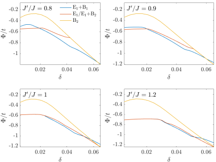
Figure 14: Dependence of the free energies on $\delta$ of the most favorable pairing states found in the SCE analysis.

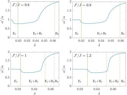
Figure 15: Dependence of the parameters in the E₁+B₁ order parameter (Eq. (23)), $\alpha^{\prime}/\alpha$, on $\delta$ for different $J^{\prime}/J$. The first (dotted green line) and second (solid green line) order transitions separating the superconducting states are found from the free energy analysis of Fig. 14.

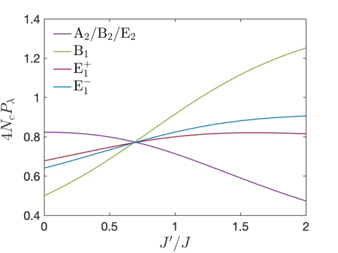
Figure 16: Triplet pairing correlations dependence on $J^{\prime}/J$ of the half-filled Hubbard model (2) on a six-site cluster. Note that the degeneracy of the E${}_{1}^{-}$ and E${}_{1}^{+}$ is lifted on the six-site cluster at this has C_2v symmetry rather than the C_6v symmetry of the full lattice. Nevertheless we retain the C_6v labels to retain straightforward connection to the rest of the manuscript.

As a relevant example to the phase diagrams of Fig. 4, we evaluate the matrix elements taking $\lambda=\text{E}_{1}$ since this is the most favorable pure state, i.e., the irreducible representation with the highest $T_{c}$ for large ${\tilde{J}}$ for $J^{\prime}/J=1$ or $1.5$ (see Fig. 8 and 9). The dependence of matrix elements on $J^{\prime}/J$ for $T=0.01t$ and a fixed hole doping of $\delta=0.05$ is shown in Fig. 13. We first note that while matrix elements between E₁ and B₁ or B₂ states are non-zero, there is no hybridization with A₂ and E₂ states. This shows that hybrid $p+f$ (E₁+B₁ or E₁+B₂) states are allowed below $T_{c}$ but $p+d$ (E₁+E₂) and $p+i$ (E₁+A₂) states are not. This is consistent with the phase diagrams, Fig. 4. Since the E₁/B₁ hybridization is comparable to the E₁/B₂ around $J^{\prime}=J$ we can expect both combinations to occur. On the other hand, although around $J^{\prime}=1.5J$ the E₁/B₁ hybridization is strong, it is the E₁ solution that wins in the SCE analysis as Fig. 4 shows.

The analysis above is then useful to predict which pairing states may combine below $T_{c}$ due to spontaneous symmetry breaking in the most favorable channel. This can be done before getting into the solution of the numerically cumbersome SCEs.

We now provide more details about the hybrid superconducting states obtained from the full SCEs. In Fig. 14 we compare the free energies of the most favorable states around $J^{\prime}/J=1$ where the hybrid superconducting states are stabilised consistent with the weak coupling analysis just provided above. For $J^{\prime}/J=0.8$ and $J^{\prime}/J=0.9$ the E₁+B₁ state has the lowest energy in the doping range $0.02<\delta<0.06$ sandwiched between an $E_{1}$ and a $B_{2}$. On the other hand, for $J^{\prime}/J=1$ and $J^{\prime}/J=1.2$, the E₁+B₂ hybrid state is most favorable between the E₁+B₁ and the B₂. A first order transition from the E₁+B₁ to the E₁ solution occurs at $\delta\sim 0.02$ for $J^{\prime}/J=0.8,0.9$, which becomes second order for $J^{\prime}/J=1,1.2$ consistent with the behavior shown in the phase diagrams of Fig.4.

Finally we consider in detail the properties of the E₁+B₁ state which is the most robust hybrid superconducting state found in the SCE. The dependence of $\alpha^{\prime}/\alpha$ ratios describing the mixed E₁+B₁ gap function (Eq. (23)) is plotted in Fig. 15 for the same $J^{\prime}/J$ as shown in Fig. 14. The smooth variation of $\alpha^{\prime}/\alpha$ with $\delta$ indicates that the hybrid E₁+B₁ state is not an artifact of the numerical solution of the SCE. Superconducting transitions occur concomitantly with the phase transitions identified from the free energies plotted in Fig 14 as expected.

Appendix D Pairing correlations from exact diagonalization on small clusters

Following our previous work [36] we explore unconventional triplet pairing using ED techniques on the half-filled Hubbard model with imaginary hopping amplitudes (2). As explained in Sec. II this model, at half-filling, maps onto the easy-plane ferromagnetic XXZ model (3). We have checked through ED calculations that indeed the two models share the same ground state for $U\gg t,t^{\prime}$.

In order to elucidate the pairing symmetry of the tRVB state as $\delta\rightarrow 0$ we compute the pairing correlations which can be obtained exactly by evaluating[59]:

$$P_{\lambda}=\frac{1}{4N_{c}}\sum_{\langle\alpha i,\beta j\rangle}\sum_{\langle\gamma k,\delta l\rangle}\Delta_{\alpha i,\beta j}(\lambda)\Delta_{\gamma k,\delta l}(\lambda)\left(\langle c_{\alpha i\uparrow}^{\dagger}c_{\beta j\downarrow}^{\dagger}c_{\gamma k\uparrow}c_{\delta l\downarrow}\rangle-\langle c^{\dagger}_{\alpha i\uparrow}c_{\gamma k\uparrow}\rangle\langle c^{\dagger}_{\beta j\downarrow}c_{\delta l\downarrow}\rangle\right)$$ (56)

where $N_{c}=6$, $\alpha,\beta,\gamma,\delta=A,B$, $i,j,k,l=1,2,3$ and $\lambda=1,...,9$. The nine-component vector $\Delta_{\lambda}$ contains the pairing solutions obtained from the linearized equations of Sec. IV.4 which are described in Appendix A. The correspondence between the vector components of ${\bf\Delta}$ and the Cooper paired bonds $(\alpha i,\beta j)$ are indicated in Eq. (12). As well as the expected value of the product of the creation and annihilation pairing operators, note that there is a substracted term which suppresses the contribution from the $i=j$ pairing amplitudes. Although these are substantial in small clusters, they are less important for quantifying actual superconducting correlations in the extended lattice.

Fig. 16 illustrates the dependence of the triplet pairing correlations of the half-filled Hubbard model (2) on a six-site cluster with $J^{\prime}/J\propto\lambda^{\prime 2}/\lambda^{2}$. The largest pairing correlations in a given channel, $\lambda$, $P_{\lambda}$, indicates that it is the most favorable at a given $J^{\prime}/J$. The pairing correlations associated with the spatial symmetries A₂, B₂ and E₂ are degenerate in the whole $J^{\prime}/J$ range explored due to the absence of intertriangle pairing amplitudes in these solutions making them indistinguishable on a six-site cluster. The results of Fig. 16 show that while the A₂, B₂ and E₂ solutions are favored for $J^{\prime}/J\leq 1/\sqrt{2}$, the $B_{1}$ followed by an $E_{1}$ dominates for $J^{\prime}/J>1/\sqrt{2}$. This change of solutions with $J^{\prime}/J$ is in overall qualitative agreement with the predictions of the linearized gap equations, Fig. 12.

Appendix E Chern number in superconducting states

In a discretized Brillouin zone, the total Chern number $\nu$ can be calculated from the Berry phases $\gamma_{nl}$ at each elementary placquette $l$. The Berry phase is the accumulated phase of the wave function along a closed $k$-path.

$$\gamma_{nl}=\imaginary\ln\prod_{j=0}^{N-1}\bra{u_{\bf{nk}_{j}}}\ket{u_{\bf{nk}_{j+1}}}$$ (57)

where $n$ is the band index and the loop chosen is rectangular with $N=4$. In the multiband case the wave functions overlap of all possible combinations must be taken into account. Thus we construct a $N_{c}\times N_{c}$ matrix at each step of the path, where $N_{c}$ is the number of occupied bands,. Then, the Berry phase is just the phase of the determinant of the product of these matrices along the loop. The Chern number is the sum over the first Brillouin zone (FBZ) of all those Berry phases:

$$\nu=\frac{1}{2\pi}\sum_{FBZ}\imaginary\ln\det\prod_{j=0}^{3}\bra{u_{\bf{mk}_{j}}}\ket{u_{\bf{nk}_{j+1}}}$$ (58)

where $1\leq m,n\leq N_{c}$.

The Chern number $\nu$ of a 2-dimensional superconductor with broken time-reversal symmetry can be computed following the exact procedure stated above but replacing $\ket{u_{nk}}$ by the Bogoliubov quasiparticle wave functions.[60]

References

- Norman et al. [2005] M. R. Norman, D. Pines, and C. Kallin, The pseudogap: friend or foe of high Tc?, Adv. Phys. 54, 715 (2005).
- Lee et al. [2006] P. A. Lee, N. Nagaosa, and X.-G. Wen, Doping a mott insulator: Physics of high-temperature superconductivity, Rev. Mod. Phys. 78, 17 (2006).
- Ogata and Fukuyama [2008] M. Ogata and H. Fukuyama, The t-J model for the oxide high-Tc superconductors, Rep. Prog. Phys. 71, 036501 (2008).
- Powell and McKenzie [2011] B. J. Powell and R. H. McKenzie, Quantum frustration in organic mott insulators: from spin liquids to unconventional superconductors, Rep. Prog. Phys. 74, 056501 (2011).
- Cao et al. [2018a] Y. Cao, V. Fatemi, A. Demir, S. Fang, S. L. Tomarken, J. Y. Luo, J. D. Sanchez-Yamagishi, K. Watanabe, T. Taniguchi, E. Kaxiras, R. C. Ashoori, and P. Jarillo-Herrero, Correlated insulator behaviour at half-filling in magic-angle graphene superlattices, Nature 556, 80 (2018a).
- Cao et al. [2018b] Y. Cao, V. Fatemi, S. Fang, K. Watanabe, T. Taniguchi, E. Kaxiras, and P. Jarillo-Herrero, Unconventional superconductivity in magic-angle graphene superlattices, Nature 556, 43 (2018b).
- McKenzie [1997] R. H. McKenzie, Similarities between organic and cuprate superconductors, Science 278, 820 (1997).
- Kurosaki et al. [2005] Y. Kurosaki, Y. Shimizu, K. Miyagawa, K. Kanoda, and G. Saito, Mott transition from a spin liquid to a fermi liquid in the spin-frustrated organic conductor , Phys. Rev. Lett. 95, 177001 (2005).
- Shimizu et al. [2016] Y. Shimizu, T. Hiramatsu, M. Maesato, A. Otsuka, H. Yamochi, A. Ono, M. Itoh, M. Yoshida, M. Takigawa, Y. Yoshida, and G. Saito, Pressure-tuned exchange coupling of a quantum spin liquid in the molecular triangular lattice , Phys. Rev. Lett. 117, 107203 (2016).
- Anderson [1987] P. W. Anderson, The resonating valence bond state in La2CuO4 and superconductivity, Science 235, 1196 (1987).
- Powell and McKenzie [2007] B. J. Powell and R. H. McKenzie, Symmetry of the superconducting order parameter in frustrated systems determined by the spatial anisotropy of spin correlations, Phys. Rev. Lett. 98, 027005 (2007).
- Anderson [1973] P. Anderson, Resonating valence bonds: A new kind of insulator?, Mater. Res. Bull. 8, 153 (1973).
- Balents et al. [2020] L. Balents, C. Dean, D. Efetov, and Y. A. F., Superconductivity and strong correlations in moiré flat bands, Nat. Phys. 16, 725–733 (2020).
- Leggett [2004] A. J. Leggett, Nobel lecture: Superfluid : the early days as seen by a theorist, Rev. Mod. Phys. 76, 999 (2004).
- Leggett [1975] A. J. Leggett, A theoretical description of the new phases of liquid , Rev. Mod. Phys. 47, 331 (1975).
- Mackenzie et al. [2017] A. P. Mackenzie, T. Scaffidi, C. W. Hicks, and Y. Maeno, Even odder after twenty-three years: the superconducting order parameter puzzle of Sr2RuO4, npj Quantum Mater. 2, 40 (2017).
- Mackenzie and Maeno [2003] A. P. Mackenzie and Y. Maeno, The superconductivity of and the physics of spin-triplet pairing, Rev. Mod. Phys. 75, 657 (2003).
- Pustogow et al. [2019] A. Pustogow, Y. Luo, A. Chronister, Y.-S. Su, D. A. Sokolov, F. Jerzembeck, A. P. Mackenzie, C. W. Hicks, N. Kikugawa, S. Raghu, E. D. Bauer, and S. E. Brown, Constraints on the superconducting order parameter in from oxygen-17 nuclear magnetic resonance, Nature 574, 72 (2019).
- Wosnitza [2019] J. Wosnitza, Superconductivity of organic charge-transfer salts, J. Low Temp. Phys. 197, 250 (2019).
- Bao et al. [2015] J.-K. Bao, J.-Y. Liu, C.-W. Ma, Z.-H. Meng, Z.-T. Tang, Y.-L. Sun, H.-F. Zhai, H. Jiang, H. Bai, C.-M. Feng, Z.-A. Xu, and G.-H. Cao, Superconductivity in quasi-one-dimensional with significant electron correlations, Phys. Rev. X 5, 011013 (2015).
- Yang et al. [2021] J. Yang, J. Luo, C. Yi, Y. Shi, Y. Zhou, and G. qing Zheng, Spin-triplet superconductivity in , Sci. Adv. 7, eabl4432 (2021).
- Cai et al. [2020] W. Cai, H. Sun, W. Xia, C. Wu, Y. Liu, H. Liu, Y. Gong, D.-X. Yao, Y. Guo, and M. Wang, Pressure-induced superconductivity and structural transition in ferromagnetic , Phys. Rev. B 102, 144525 (2020).
- König et al. [2022] E. J. König, Y. Komijani, and P. Coleman, Triplet resonating valence bond theory and transition metal chalcogenides, Phys. Rev. B 105, 075142 (2022).
- Lin Jiao et al. [2020] S. H. Lin Jiao, S. Ran, Z. Wang, J. O. Rodriguez, M. Sigrist, Z. Wang, N. P. Butch, and V. Madhavan, Chiral superconductivity in heavy-fermion metal UTe2, Nature 579, 523–527 (2020).
- Aoki et al. [2019] D. Aoki, K. Ishida, and J. Flouquet, Review of u-based ferromagnetic superconductors: Comparison between UGe2, urhge, and ucoge, Journal of the Physical Society of Japan 88, 022001 (2019), https://doi.org/10.7566/JPSJ.88.022001 .
- Coleman et al. [2020] P. Coleman, Y. Komijani, and E. J. König, Triplet resonating valence bond state and superconductivity in hund’s metals, Phys. Rev. Lett. 125, 077001 (2020).
- Anderson [1985] P. W. Anderson, Further consequences of symmetry in heavy-electron superconductors, Phys. Rev. B 32, 499 (1985).
- Baudron et al. [2005] S. A. Baudron, P. Batail, C. Coulon, R. Clérac, E. Canadell, V. Laukhin, R. Melzi, P. Wzietek, D. Jérome, P. Auban-Senzier, and S. Ravy, (edt-ttf-conh2)6[re6se8(cn)6], a metallic kagome-type organic–inorganic hybrid compound: Electronic instability, molecular motion, and charge localization, Journal of the American Chemical Society 127, 11785 (2005), pMID: 16104757, https://doi.org/10.1021/ja0523385 .
- Llusar et al. [2004] R. Llusar, S. Uriel, C. Vicent, J. M. Clemente-Juan, E. Coronado, C. J. Gómez-García, B. Braïda, and E. Canadell, Single-component magnetic conductors based on Mo3S7 trinuclear clusters with outer dithiolate ligands, J. Am. Chem. Soc. 126, 12076 (2004).
- Shuku et al. [2018] Y. Shuku, A. Mizuno, R. Ushiroguchi, C. S. Hyun, Y. J. Ryu, B.-K. An, J. E. Kwon, S. Y. Park, M. Tsuchiizu, and K. Awaga, An exotic band structure of a supramolecular honeycomb lattice formed by a pancake – interaction between triradical trianions of triptycene tribenzoquinone, Chem. Commun. 54, 3815 (2018).
- López and Merino [2020] M. F. López and J. Merino, Magnetism and topological phases in an interacting decorated honeycomb lattice with spin-orbit coupling, Phys. Rev. B 102, 035157 (2020).
- Nourse et al. [2021a] H. L. Nourse, R. H. McKenzie, and B. J. Powell, Multiple insulating states due to the interplay of strong correlations and lattice geometry in a single-orbital hubbard model, Phys. Rev. B 103, L081114 (2021a).
- Nourse et al. [2021b] H. L. Nourse, R. H. McKenzie, and B. J. Powell, Spin-0 mott insulator to metal to spin-1 mott insulator transition in the single-orbital hubbard model on the decorated honeycomb lattice, Phys. Rev. B 104, 075104 (2021b).
- Fernández López and Merino [2022] M. Fernández López and J. Merino, Bad topological semimetals in layered honeycomb compounds, Phys. Rev. B 105, 115138 (2022).
- Nourse et al. [2022] H. L. Nourse, R. H. McKenzie, and B. J. Powell, symmetry breaking metal-insulator transitions in a flat band in the half-filled hubbard model on the decorated honeycomb lattice, Phys. Rev. B 105, 205119 (2022).
- Merino et al. [2021] J. Merino, M. F. López, and B. J. Powell, Unconventional superconductivity near a flat band in organic and organometallic materials, Phys. Rev. B 103, 094517 (2021).
- Khosla et al. [2017] A. L. Khosla, A. C. Jacko, J. Merino, and B. J. Powell, Spin-orbit coupling and strong electronic correlations in cyclic molecules, Phys. Rev. B 95, 115109 (2017).
- Jacko et al. [2017] A. C. Jacko, A. L. Khosla, J. Merino, and B. J. Powell, Spin-orbit coupling in , Phys. Rev. B 95, 155120 (2017).
- Merino et al. [2017] J. Merino, A. C. Jacko, A. L. Khosla, and B. J. Powell, Effects of anisotropy in spin molecular-orbital coupling on effective spin models of trinuclear organometallic complexes, Phys. Rev. B 96, 205118 (2017).
- Powell et al. [2017] B. J. Powell, J. Merino, A. L. Khosla, and A. C. Jacko, Heisenberg and dzyaloshinskii-moriya interactions controlled by molecular packing in trinuclear organometallic clusters, Phys. Rev. B 95, 094432 (2017).
- Rachel and Le Hur [2010] S. Rachel and K. Le Hur, Topological insulators and mott physics from the hubbard interaction, Phys. Rev. B 82, 075106 (2010).
- Trebst and Hickey [2022] S. Trebst and C. Hickey, Kitaev materials, Physics Reports 950, 1 (2022).
- Winter et al. [2017] S. M. Winter, A. A. Tsirlin, M. Daghofer, J. van den Brink, Y. Singh, P. Gegenwart, and R. Valentí, Models and materials for generalized kitaev magnetism, Journal of Physics: Condensed Matter 29, 493002 (2017).
- Hazra and Coleman [2022] T. Hazra and P. Coleman, Triplet pairing mechanisms from Hund’s-Kondo models: applications to UTe2 and CeRh2As2 10.48550/arxiv.2205.13529 (2022).
- Jacko et al. [2015] A. C. Jacko, C. Janani, K. Koepernik, and B. J. Powell, Emergence of quasi-one-dimensional physics in a nearly-isotropic three-dimensional molecular crystal: Ab initio modeling of , Phys. Rev. B 91, 125140 (2015).
- Shindou and Momoi [2009] R. Shindou and T. Momoi, slave-boson formulation of spin nematic states in frustrated ferromagnets, Phys. Rev. B 80, 064410 (2009).
- Moessner and Raman [2011] R. Moessner and K. S. Raman, Quantum dimer models. In C Lacroix, P Mendels, F Mila (Eds.). Introduction to frustrated magnetism: Materials, experiments, theory (Springer, Berlin, Heidelberg, 2011) Chap. 17, pp. 437–479.
- Powell [2020] B. J. Powell, Emergent particles and gauge fields in quantum matter, Contemporary Physics 61, 96 (2020), https://doi.org/10.1080/00107514.2020.1832350 .
- Jahromi and Orús [2018] S. S. Jahromi and R. Orús, Spin- heisenberg antiferromagnet on the star lattice: Competing valence-bond-solid phases studied by means of tensor networks, Phys. Rev. B 98, 155108 (2018).
- Kaba and Sénéchal [2019] S.-O. Kaba and D. Sénéchal, Group-theoretical classification of superconducting states of strontium ruthenate, Phys. Rev. B 100, 214507 (2019).
- Note [1] The -wave superconducting state found in our previous paper [36] was incorrectly labeled as a B2 but is in fact a B1 (both are -wave states). The nodal structure corresponds to an cubic basis function.
- Kotliar and Liu [1988] G. Kotliar and J. Liu, Superexchange mechanism and d-wave superconductivity, Phys. Rev. B 38, 5142 (1988).
- Powell [2008] B. J. Powell, A phenomenological model of the superconducting state of the bechgaard salts, Journal of Physics: Condensed Matter 20, 345234 (2008).
- Vollhardt and Wolfle [1990] D. Vollhardt and P. Wolfle, The superfluid phases of helium 3 (CRC Press, 1990).
- Sigrist and Ueda [1991] M. Sigrist and K. Ueda, Phenomenological theory of unconventional superconductivity, Rev. Mod. Phys. 63, 239 (1991), pages 250-251.
- You et al. [2012] Y.-Z. You, I. Kimchi, and A. Vishwanath, Doping a spin-orbit mott insulator: Topological superconductivity from the kitaev-heisenberg model and possible application to (Na2/Li2)IrO3, Phys. Rev. B 86, 085145 (2012).
- Powell [2006] B. J. Powell, Mixed order parameters, accidental nodes and broken time reversal symmetry in organic superconductors: a group theoretical analysis, Journal of Physics: Condensed Matter 18, L575 (2006).
- Oike et al. [2017] H. Oike, Y. Suzuki, H. Taniguchi, Y. Seki, K. Miyagawa, and K. Kanoda, Anomalous metallic behaviour in the doped spin liquid candidate -(ET)4Hg2.89Br8, Nat. Commun. 8, 756 (2017).
- Merino and Gunnarsson [2014] J. Merino and O. Gunnarsson, Pseudogap and singlet formation in organic and cuprate superconductors, Phys. Rev. B 89, 245130 (2014).
- Lee et al. [2019] K. Lee, T. Hazra, M. Randeria, and N. Trivedi, Topological superconductivity in dirac honeycomb systems, Phys. Rev. B 99, 184514 (2019).