GAN you hear me?
Reclaiming unconditional speech synthesis from diffusion models

Abstract

We propose AudioStyleGAN (ASGAN), a new generative adversarial network (GAN) for unconditional speech synthesis. As in the StyleGAN family of image synthesis models, ASGAN maps sampled noise to a disentangled latent vector which is then mapped to a sequence of audio features so that signal aliasing is suppressed at every layer. To successfully train ASGAN, we introduce a number of new techniques, including a modification to adaptive discriminator augmentation to probabilistically skip discriminator updates. ASGAN achieves state-of-the-art results in unconditional speech synthesis on the Google Speech Commands dataset. It is also substantially faster than the top-performing diffusion models. Through a design that encourages disentanglement, ASGAN is able to perform voice conversion and speech editing without being explicitly trained to do so. ASGAN demonstrates that GANs are still highly competitive with diffusion models. Code, models, samples: https://github.com/RF5/simple-asgan/.

Index Terms—  Unconditional speech synthesis, generative adversarial networks, speech disentanglement, voice conversion.

1 Introduction

Unconditional speech synthesis is the task of generating coherent speech without any conditioning inputs such as text or speaker labels [1]. As in image synthesis [2], a well-performing unconditional speech synthesis model would have several useful applications: from latent interpolations between utterances and fine-grained tuning of different aspects of the generated speech, to audio compression and better probability density estimation of speech.

Spurred on by recent improvements in diffusion models [3] for images [4, 5, 6], there has been a substantial improvement in unconditional speech synthesis in the last few years. The current best-performing approaches are all trained as diffusion models [7, 8]. Before this, most studies used generative adversarial networks (GANs) [9] that map a latent vector to a sequence of speech features with a single forward pass through the model. However, performance was limited [1, 10], leading to GANs falling out of favour for this task.

Motivated by the StyleGAN literature [11, 12, 13] for image synthesis, we aim to reinvigorate GANs for unconditional speech synthesis. To this end, we propose AudioStyleGAN (ASGAN): a convolutional GAN which maps a single latent vector to a sequence of audio features, and is designed to have a disentangled latent space. The model is based in large part on StyleGAN3 [13], which we adapt for audio synthesis. Concretely, we adapt the style layers to remove signal aliasing caused by the non-linearities in the network. This is accomplished with anti-aliasing filters to ensure that the Nyquist$\mathchar 45\relax$Shannon sampling limits are met in each layer. We also propose a modification to adaptive discriminator augmentation [14] to stabilize training by randomly dropping discriminator updates based on a guiding signal.

Using objective metrics to measure the quality and diversity of generated samples [15, 2, 16], we show that ASGAN sets a new state-of-the-art in unconditional speech synthesis on the Google Speech Commands digits dataset [17]. It not only outperforms the best existing models, but is also faster to train and faster in inference. Mean opinion scores (MOS) also indicate that ASGAN’s generated utterances sound more natural (MOS: 3.68) than the existing best model (SaShiMi [7], MOS: 3.33).

Through ASGAN’s design, the model’s latent space is disentangled during training, enabling the model – without any additional training – to also perform voice conversion and speech editing in a zero-shot fashion. Objective metrics that measure latent space disentanglement indicate that ASGAN has smoother latent representations compared to existing diffusion models.

2 Related work

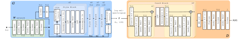
Fig. 1: The ASGAN generator (left) and discriminator (right). FF, LPF, Conv1D indicate Fourier feature [13], low-pass filter, and 1D convolution layers, respectively. The numbers above linear and convolutional layers indicate the number of output features/channels for that layer. Stacked blocks indicate a layer repeated sequentially, with the number of repeats indicated above the block (e.g. “x3”).

We start by distinguishing what we call unconditional speech synthesis to the related but different task of generative spoken language modeling (GSLM). In GSLM, a large autoregressive language model is typically trained on some discrete units (e.g. HuBERT [18] clusters or clustered spectrogram features), similar to how a language model is trained on text [19, 20]. While this also enables the generation of speech without any conditioning input, GSLM implies a model structure consisting of an encoder to discretize speech, a language model, and a decoder [21]. This means that during generation, you are bound by the discrete units in the model. E.g., it is not possible to interpolate between two utterances in a latent space or to directly control speaker characteristics during generation. If this is desired, additional components must be explicitly built into the model [20].

In contrast, in unconditional speech synthesis we do not assume any knowledge of particular aspects of speech beforehand. Instead of using some intermediate discretization step, such models typically use noise to directly generate speech, often via some latent representation. The latent space should ideally be disentangled, allowing for modelling and control of the generated speech. In contrast to GSLM, the synthesis model should learn to disentangle without being explicitly designed to control specific speech characteristics. In some sense this is a more challenging task than GSLM, which is why most unconditional speech synthesis models are still evaluated on short utterances of isolated spoken words [1] (as we also do here).

Within unconditional speech synthesis, a substantial body of work focuses on either autoregressive [22] models – generating a current sample based on previous outputs – or diffusion models [8]. Diffusion models iteratively de-noise a sampled signal into a waveform through a Markov chain with a constant number of steps [3]. At each inference step, the original noise signal is slightly de-noised until – in the last step – it resembles coherent speech. Autoregressive and diffusion models are relatively slow because they require repeated forward passes through the model during inference.

Earlier studies [1, 10] attempted to use GANs [9] for unconditional speech synthesis, which has the advantage of requiring only a single pass through the model. While results showed some initial promise, performance was poor in terms of speech quality and diversity, with the more recent diffusion models performing much better [7]. However, there have been substantial improvements in GAN-based modelling for image synthesis in the intervening years [14, 11, 12]. Our goal is to improve the performance of the earlier GAN-based unconditional speech synthesis models by adapting lessons from these recent image synthesis studies.

Some of these innovations in GANs are modality-agnostic: $R_{1}$ regularization [23] and exponential moving averaging of generator weights [24] can be directly transferred from the vision domain to speech. Other techniques, such as the carefully designed anti-aliasing filters between layers in StyleGAN3 [13] require specific adaptation; in contrast to images, there is little meaningful information in speech below 300 Hz, necessitating a redesign of the anti-aliasing filters.

In a very related research direction, Beguš [25, 10] has been studying how GAN-based unconditional speech synthesis models internally perform lexical and phonological learning, and how this relates to human learning. These studies, however, have been relying on the older GAN synthesis models. We hope that by developing better performing GANs for unconditional speech synthesis, such investigations will also be improved. Recently, [26] attempted to directly use StyleGAN2 for conditional and unconditional synthesis of emotional vocal bursts. This further motivates a reinvestigation of GANs, but here we look specifically at the generation of speech rather than paralinguistic sounds.

3 ASGAN: Audio Style GAN

Our model is based on the StyleGAN family of models [11] for image synthesis. We adapt and extend the approach to audio, and therefore dub our model AudioStyleGAN (ASGAN). The model follows the setup of a standard GAN with a single generator network $G$ and a single discriminator $D$ [9]. The generator $G$ accepts a vector $\mathbf{z}$ sampled from a normal distribution and processes it into a sequence of speech features $X$. In this work, we restrict the sequence of speech features $X$ to always have a fixed pre-specified duration. The discriminator $D$ accepts a sequence of speech features $X$ and yields a scalar output. $D$ is optimized to raise its output for $X$ sampled from real data and lower its output for $X$ produced by the generator. Meanwhile, $G$ is optimized to maximize $D(X)$ for $X$ sampled from the generator, i.e. when $X=G(\mathbf{z})$. The features $X$ are converted to a waveform using a pretrained HiFi-GAN vocoder [27]. During training, a new adaptive discriminator updating technique is added to ensure stability and convergence, as discussed in Sec. 4.

3.1 Generator

The architecture of the generator $G$ is shown on the left of Fig. 1. It consists of a latent mapping network $W$ that converts $\mathbf{z}$ to a disentangled latent space, a special Fourier feature (FF) layer which converts a single vector from this latent space into a sequence of cosine features of fixed length, and finally a convolutional encoder which iteratively refines the cosine features into the final speech features $X$.

Mapping network: The mapping network $W$ is a multi-layer perceptron with leaky ReLU activations. As input it takes in a vector sampled from a normal distribution $\mathbf{z}\sim Z=\mathcal{N}(\mathbf{0},\mathbf{I})$; we use a 512-dimensional multi-variate normal vector, $\mathbf{z}\in\mathbb{R}^{512}$. Passing $\mathbf{z}$ through the mapping network produces a latent vector $\mathbf{w}=W(\mathbf{z})$ of the same dimensionality as $\mathbf{z}$. As explained in [11], the primary purpose of $W$ is to learn to map noise to a linearly disentangled space, as this will allow for controllable and understandable synthesis. $W$ is coaxed into learning such a disentangled representation because it can only linearly modulate channels of the cosine features in each layer of the convolutional encoder (see details below). This means that $W$ must learn to map the random normal $Z$-space into a $W$-space that linearly disentangles common factors of speech variation.

Convolutional encoder: The convolutional encoder begins by linearly projecting $\mathbf{w}$ as the input to an FF layer [28]. We use the Gaussian Fourier feature mapping [28] and incorporate the transformation from StyleGAN3 [13]. The Gaussian FF layer samples a frequency and phase from a Gaussian distribution for each output channel. The layer then linearly projects the input vector to a vector of phases which are added to the random phases. The output is calculated as the cosine functions of these frequencies and phases, one frequency/phase for each output channel. The result is that $\mathbf{w}$ is converted into a sequence of vectors at the output of the FF layer. This is iteratively passed through several Style Blocks. In each Style Block layer, the input sequence is passed through a modulated convolution layer [12] whereby the final convolution kernel is computed by multiplying the layer’s learnt kernel with the style vector derived from $\mathbf{w}$, broadcasted over the length of the kernel. To ensure the signal does not experience aliasing due to the non-linearity, the leaky ReLU layers are surrounded by layers responsible for anti-aliasing (explained below). All these layers comprise a Style Block, which is repeated in groups of 5, 4, 3, and finally 2 blocks. The last block in each group upsamples by $4\times$ instead of $2\times$, thereby increasing the sequence length by a factor of 2 for each group. A final 1D convolution projects the output from the last group into the audio feature space (e.g. log mel-spectrogram or HuBERT features [18]), as illustrated in the middle of Fig. 1.

Anti-aliasing filters: From image synthesis with GANs [13], we know that the generator must include anti-aliasing filters for the signal propagating through the network to satisfy the Nyquist-Shannon sampling theorem. This is why, before and after a non-linearity, we include upsampling, low-pass filter (LPF), and downsampling layers in each Style Block. The motivation from [13] is that most non-linearities introduce arbitrarily high-frequency information into the output signal. The signal we are modelling (speech) is continuous, and the internal discrete-time features that are passed through the network is therefore a digital representation of this continuous signal. From the Nyquist-Shannon sampling theorem, we know that for such a discrete-time signal to accurately reconstruct the continuous signal, it must be bandlimited to $0.5\text{\,}\text{cycles/sample}$. If not, the generator can learn to use aliasing artifacts to fool the discriminator, to the detriment of the quality and control of the final output. To address this, we follow [13]: we approximate an ideal continuous LPF through the sequence of upsample, LPF, non-linearity, and downsample operations to ensure that the signal is bandlimited. We reason that the generator should ideally first focus on generating course features before generating good high-frequency details, which will inevitably contain more trace aliasing artifacts. So we design the filter cutoff to begin at a small value in the first Style Block, and increase gradually to near the critical Nyquist frequency in the final block.

3.2 Discriminator

The discriminator $D$ has a convolutional architecture similar to [12], taking a sequence of speech features $X$ as input and predicting whether it is generated by $G$ or sampled from the dataset. Concretely, $D$ consists of four ConvD Blocks and a network head, as show in Fig. 1. Each ConvD Block is comprised of 1D convolutions with skip connections, and a downsampling layer with an anti-aliasing LPF in the last skip connection. The LPF cutoff is set as the Nyquist frequency for all layers. The number of layers and channels are chosen so that $D$ has roughly the same number of parameters as $G$. $D$’s head consists of a minibatch standard deviation [24] layer and a 1D convolution layer before passing the flattened activations through a final linear projection head to arrive at the logits. Both $D$ and $G$ are trained using the non-saturating logistic loss [9].

3.3 Vocoder

Once the generator $G$ and discriminator $D$ are trained, we need a way to convert the speech features back to waveforms. For this we use a pretrained HiFi-GAN vocoder [27] that vocodes either log mel-scale spectrograms or HuBERT features [18].

4 Experimental Setup

4.1 Data

To compare to existing unconditional speech synthesis models, we use the Google Speech Commands dataset of isolated spoken words [17]. As in other studies [7, 8, 1], we use the subset corresponding to the ten spoken digits “zero” to “nine” (called SC09). The digits are spoken by various speakers under different channel conditions. This makes it a challenging benchmark for unconditional speech synthesis. All utterances are roughly a second long and are sampled at 16 kHz.

4.2 Evaluation metrics

We train and validate our models on the official training split from SC09. We then evaluate speech synthesis quality by seeing how well newly generated utterances match the distribution of the SC09 test split. We use metrics similar to those for image synthesis; they measure either the quality of generated utterances (realism compared to test data), or the diversity of generated utterances (how varied the utterances are relative to the test set), or a combination of both.

These metrics require extracting features or predictions from a supervised speech classifier network trained to classify the utterances from SC09. While there is no consistent pretrained classifier used for this purpose, we opt to use a ResNeXT architecture [29], similar to previous studies [7, 8]. The trained model has a 98.1% word classification accuracy on the SC09 test set, and we make the model available for future comparisons. Using either the classification output or 1024-dimensional features extracted from the penultimate layer in the classifier, we consider the following metrics.

Inception score (IS) measures the diversity and quality of generated samples by evaluating the Kullback-Leibler (KL) divergence between the label distribution from the classifier output and the mean label distribution over a set of generated utterances [15]. Modified Inception score (mIS) extends IS by incorporating a measure of intra-class diversity (in our case over the ten digits) to reward models with a higher intra-class entropy [30]. Fréchet Inception distance (FID) computes a measure of how well the distribution of generated utterances matches the train-set utterances by comparing the classifier features of generated and real data [2]. Activation maximization (AM) measures generator quality by comparing the KL divergence between the classifier class probabilities from real and generated data, while penalizing high classifier entropy samples produced by the generator [16]. Intuitively, this attempts to account for class imbalance in the training set and also intra-class diversity. All these metrics have been used in previous unconditional speech synthesis studies [7, 8].

A major motivation for ASGAN’s design is latent-space disentanglement. To evaluate this, we use two disentanglement metrics on the latent $Z$-space and $W$-space. Path length measures the mean $L_{2}$ distance moved by the classifier features when the latent point ($\mathbf{z}$ or $\mathbf{w}$) is randomly perturbed slightly, averaged over many perturbations [11]. A lower value indicates a smoother latent space. Linear separability utilizes a linear support vector machine (SVM) to classify the digit of a latent point. The metric is computed as the additional information (in terms of mean entropy) necessary to correctly classify an utterance (in terms of which digit is spoken) [11]. Again, a lower value indicates a more linearly disentangled latent space. These metrics are averaged over 5000 generated utterances for each model. As in [11], for linear separability we exclude half the generated utterances for which the ResNeXT classifier is least confident.

Finally, to give an indication of naturalness, we compute an estimated mean opinion score (eMOS) using a pretrained Wav2Vec2 small baseline from the recent VoiceMOS challenge [31]. This model is trained to predict the naturalness score that a human would assign to an utterance from 1 (least natural) to 5 (most natural). We also perform a subjective MOS evaluation using the same scale. Concretely, we utilize Amazon Mechanical Turk to obtain 240 opinion scores for each model with 12 speakers listening to each utterance.

4.3 Baselines

We compare to the following unconditional speech synthesis methods (Sec. 2): WaveGAN [1], DiffWave [8], autoregressive SaShiMi and Sashimi+DiffWave [7] (the current best performing model on SC09). For WaveGAN we use the trained model provided by the authors [1], while for DiffWave we use an open-source pretrained model. For the autoregressive SaShiMi model, we use the code provided by the authors to train an unconditional SaShiMi model on SC09 for 1.1M updates [7]. Finally, for SaShiMi+DiffWave, we modify the autoregressive SaShiMi code and combine it with DiffWave according to [7]; we train it on SC09 for 800k updates with the parameters in the original paper [7]. In all experiments, we perform direct sampling from the latent space for the GAN and diffusion models according to the original papers. For the autoregressive models, we directly sample from the predicted output distribution for each time-step sample.

4.4 ASGAN implementation

We train two variants of our model: a log mel-spectrogram based model and a HuBERT feature based model [18]. The former is shown in Fig. 1, where the model outputs 128 mel-frequency bins at a hop and window size of 10 ms and 64 ms, respectively. The HuBERT model is identical except that it only uses half the sequence length (since HuBERT features are 20 ms instead of the 10 ms spectrogram frames) and has a different number of output channels in the four groups of Style Blocks: $[1024,768,512,512]$ convolution channels instead of $[1024,512,256,128]$.

The HiFi-GAN vocoder for both the HuBERT and mel-spectrogram model is based on the original implementation [27]. The HuBERT HiFi-GAN is trained on the Librispeech train-clean-100 subset [32] to vocode activations from layer 6 of the HuBERT Base model [18]. The mel-spectrogram HiFi-GAN is trained on the Google Speech Commands dataset.

Both ASGAN variants are trained with Adam [33] ($\beta_{1}=0,\beta_{2}=0.99$), clipping gradient norms at 10, and a learning rate of $3\cdot 10^{-3}$ for 520k iterations with a batch size of 32. Several tricks are used to stabilize GAN training: (i) equalized learning rate [24], (ii) leaky ReLU activations with $\alpha=0.1$, (iii) exponential moving averaging for the generator weights [24], (iv) $R_{1}$ regularization [23], and (v) a 0.01-times smaller learning rate for the mapping network $W$ [13].

We also introduce a new technique for updating the discriminator. Concretely, we first scale $D$’s learning rate by 0.1 compared to the generator as otherwise we find it overwhelms $G$ early on in training. Additionally we employ a dynamic method for updating $D$, inspired by adaptive discriminator augmentation [14]: during each iteration, we skip $D$’s update with probability $p$. The probability $p$ is initialized at 0.1 and is updated every 16th generator step or whenever the discriminator is updated. We keep a running average $r_{t}$ of the proportion of $D$’s outputs on real data $D(X)$ that are positive (i.e. that $D$ can confidently identify as real). Then, if $r_{t}$ is greater than 0.6 we increment $p$ by 0.05 (capped at 1.0), and if $r_{t}$ is less than 0.6 we decrease $p$ by 0.05 (capped at 0.0). In this way we adaptively skip discriminator updates. When $D$ becomes too strong, $r_{t}$ and $p$ rise, and so $D$ is updated less frequently. When $D$ becomes too weak (i.e. fails to distinguish between real and fake inputs), then the opposite happens. We found this new modification to be critical for ensuring that the $D$ does not overwhelm $G$ during training.

We also use the traditional adaptive discriminator augmentation [14] where we apply the following transforms with the same probability $p$: (i) adding Gaussian noise with $\sigma=0.05$, (ii) random scaling by a factor of $1\pm 0.05$, and (iii) randomly replacing a subsequence of frames from the generated speech features with a subsequence of frames taken from a real speech feature sequence. This last augmentation is based on the fake-as-real GAN method [34] and is important to prevent gradient explosion later in training.

For the anti-aliasing LPF filters we use windowed sinc filters with a width-9 Kaiser window [35]. For the generator, the first Style Block has a cutoff at $f_{c}=0.125\ \text{cycles/sample}$ which is increased in an even logarithmic scale to $f_{c}=0.45\ \text{cycles/sample}$ in the second-to-last layer, keeping this value for the last two layers to fill in the last high frequency detail. Even in these last layers we use a cutoff below the Nyquist frequency. For the discriminator we are less concerned about aliasing as it does not generate a sequence, so we use a $f_{c}=0.5\ \text{cycles/sample}$ cutoff for all ConvD Blocks.

All models are trained on a single NVIDIA Quadro RTX 6000 using PyTorch 1.11.

5 Results: Unconditional speech synthesis

Table 1: Results measuring the quality and diversity of generated samples from unconditional speech synthesis models together with train/test set toplines for the SC09 dataset. Subjective MOS values with 95% confidence intervals are shown.

Model	IS$\ \uparrow$	mIS $\ \uparrow$	FID$\ \downarrow$	AM$\ \downarrow$	eMOS$\ \uparrow$	MOS$\ \uparrow$
Train set	$9.37$	$237.6$	$0$	$0.20$	$2.41$	$3.74\pm 0.12$
Test set	$9.36$	$242.3$	$0.01$	$0.20$	$2.43$	$3.88\pm 0.12$
WaveGAN [1]	$4.45$	$34.6$	$1.77$	$0.81$	$1.06$	$2.88\pm 0.16$
DiffWave [8]	$5.13$	$49.6$	$1.68$	$0.68$	$1.66$	$3.43\pm 0.14$
SaShiMi [7]	$3.74$	$18.9$	$2.11$	$0.99$	$1.58$	$3.19\pm 0.15$
SaShiMi+DiffWave	$5.44$	$60.8$	$1.01$	$0.61$	$1.89$	$3.33\pm 0.12$
ASGAN (mel-spec.)	$7.02$	$162.8$	$0.56$	$0.36$	$1.76$	$3.51\pm 0.13$
ASGAN (HuBERT)	$7.67$	$226.7$	$0.14$	$0.26$	$1.99$	$3.68\pm 0.13$

Table 2: Latent-space disentanglement and speed metrics. Speed is measured as the number of samples that can be generated per unit time on a single NVIDIA Quadro RTX 6000 using a batch size of 1 given in ksamples/sec. Some models do not have a $W$-space (WaveGAN) or any continuous latent space (SaShiMi).

	Path length $\downarrow$		Separability $\downarrow$
Model	$Z$	$W$	$Z$	$W$	Speed $\uparrow$
WaveGAN [1]	1.03$\cdot\text{10}^{\text{0}}$	—	4.86	—	2214.71
DiffWave [8]	2.72$\cdot\text{10}^{\text{6}}$	7.27$\cdot\text{10}^{\text{5}}$	6.09	6.58	0.83
SaShiMi [7]	—	—	—	—	0.14
SaShiMi+DiffWave	2.89$\cdot\text{10}^{\text{6}}$	1.24$\cdot\text{10}^{\text{6}}$	4.07	2.34	0.47
ASGAN (mel-spec.)	6.77$\cdot\text{10}^{\hphantom{\text{1}}}$	3.21$\cdot\text{10}^{\hphantom{\text{1}}}$	1.81	1.01	875.45
ASGAN (HuBERT)	3.50$\cdot\text{10}^{\hphantom{\text{1}}}$	1.84$\cdot\text{10}^{\hphantom{\text{1}}}$	1.40	1.00	816.27

(a) Voice conversion

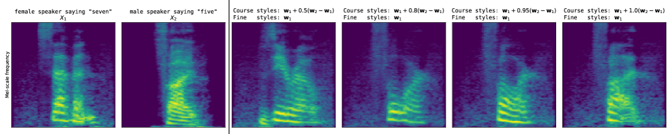
(b) Speech editing: Digit/content conversion

Fig. 2: Examples of ASGAN (HuBERT variant) performing unseen tasks on unseen speakers from the SC09 test set: (a) voice conversion and (b) speech editing. We encourage the reader to listen to audio samples at https://rf5.github.io/slt2022-asgan-demo.

Table 1 compares previous state-of-the-art unconditional speech synthesis approaches to the newly proposed ASGAN. As a reminder, IS, mIS, FID and AM measure generated speech diversity and quality relative to the test set; eMOS and MOS are measures of generated speech naturalness. We see that both variants of ASGAN outperforms the other models on most metrics. The HuBERT variant of ASGAN in particular performs best across all metrics. The improvement of the HuBERT ASGAN over the mel-spectrogram variant is likely because the high-level HuBERT speech representations make it easier for the model to disentangle common factors of speech variation. The previous best unconditional synthesis model, SaShiMi+DiffWave, still outperforms the other baseline models, and it appears to have comparable naturalness (similar eMOS and MOS) to the mel-spectrogram ASGAN variant. However, it appears to match the test set more poorly than either ASGAN variant on the other diversity metrics.

Latent space disentanglement and generation speed of each model are measured in Table 2. These results are more mixed, with WaveGAN being the fastest model and the one with the shortest latent $Z$-space path length. However, this is somewhat misleading since WaveGAN’s samples have low quality and poor diversity compared to the other models (see Table 1). This means that WaveGAN’s latent space is a poor representation of the true distribution of speech in the SC09 dataset, allowing it to have a very small path length as most paths do not span a diverse set of speech variation.

In terms of linear separability, ASGAN again yields substantial improvements over existing models. The results confirm that ASGAN has indeed learned a disentangled latent space – a primary motivation for the model’s design. Specifically, this shows that the idea from image synthesis of using the latent $\mathbf{w}$ vector to linearly modulate convolution kernels can also be applied to speech. This level of disentanglement allows ASGAN to be applied to tasks unseen during training, as described in the next section.

Regardless of performance, the speed of all the convolutional GAN models (WaveGan and ASGAN) is significantly better than the diffusion and autoregressive models. This highlights an additional benefit of utilizing convolutional GANs that produce utterances in a single inference call, as opposed to the many inference calls necessary with autoregressive or diffusion modelling.

6 Unseen tasks:
voice conversion and speech editing

To further showcase the disentangled latent space learned by ASGAN, here we qualitatively consider how it can be used to perform voice conversion and speech editing without any further training. Our goal is not to achieve state-of-the-art results on these tasks or to present a complete quantitative evaluation, but simply to illustrate the ability for our model to transfer to these unseen tasks.

For these tasks we wish to modify an already existing utterance which has not been produced by the generator $G$. To do this, we need to map the speech features back to the $G$’s latent $W$-space. This is done using a method similar to [12] whereby we optimize a $\mathbf{w}$ vector while keeping $G$ and the speech feature sequence $X$ fixed. Concretely, $\mathbf{w}$ is initialized to the mean $\bar{\mathbf{w}}=\mathbb{E}_{\mathbf{z}}[W(\mathbf{z})]$ and then fed through the network to produce a candidate sequence $\tilde{X}$. An $L_{2}$ loss between the candidate sequence $\tilde{X}$ and the target sequence $X$ is then optimized using Adam with the settings from [12].

We can modify several aspects of speech from seen or unseen speakers by performing style mixing [11]. Concretely, given speech features for two utterances $X_{1}$ and $X_{2}$ from potentially unseen speakers, we first project them to the latent space, obtaining $\mathbf{w}_{1}$ and $\mathbf{w}_{2}$. We can then use different $\mathbf{w}$ vectors as the input into each Style Block in Fig. 1. According to our design motivation in Sec. 3.1, the course styles (e.g. which word is said) are captured in the earlier layers and the fine styles (e.g. speaker identity, tone) in later layers. So, we can perform voice conversion from $X_{1}$’s speaker to $X_{2}$’s speaker by simply replacing the $\mathbf{w}$ vector in the last 5 modulated convolutions (fine styles) with $\mathbf{w}_{2}$, while using $\mathbf{w}_{1}$ in the earlier blocks (course styles). By doing the opposite, we can also do speech editing – the task of replacing the content of the words spoken (replacing $\mathbf{w}$ for course styles), but leaving the speaker identity intact (retaining $\mathbf{w}$ for fine styles). Furthermore, because the $W$-space is continuous, we can interpolate between replacing the course and fine styles to achieve varying degrees of voice conversion or speech editing.

An example of these tasks on unseen speakers on the SC09 test set is shown in Fig. 2. For these examples we use the truncation trick [11] in the $W$-space with truncation $\psi=0.3$. We encourage the reader to listen to the samples (link given in the caption).

7 Conclusion

We introduced ASGAN, a model for unconditional speech synthesis designed to learn a disentangled latent space. Specifically, we adapted existing and incorporated new GAN design and training techniques to enable ASGAN to outperform existing autoregressive and diffusion models. Experiments on the SC09 dataset validated this design, demonstrating that ASGAN outperforms previous state-of-the-art models on most metrics, while also being substantially faster. Further experiments also demonstrated the benefit of the disentangled latent space – ASGAN can, without any additional training, perform voice conversion and speech editing in a zero-shot fashion through linear operations in its latent space.

One major limitation of our work is scale: once trained, ASGAN can only generate utterances of a fixed length, and the model struggles to generate coherent full sentences on datasets with longer utterances (a limitation shared by existing unconditional synthesis models). Future work will aim to address this shortcoming by considering which aspects of ASGAN can be simplified or removed to improve scaling. Future work will also perform more thorough subjective evaluations to quantify how ASGAN performs on unseen tasks.

References

- [1] Chris Donahue, Julian McAuley, and Miller Puckette, “Adversarial audio synthesis,” in ICLR, 2018.
- [2] Martin Heusel, Hubert Ramsauer, Thomas Unterthiner, Bernhard Nessler, and Sepp Hochreiter, “GANs trained by a two time-scale update rule converge to a local Nash equilibrium,” in NeurIPS, 2017.
- [3] Jascha Sohl-Dickstein, Eric Weiss, Niru Maheswaranathan, and Surya Ganguli, “Deep unsupervised learning using nonequilibrium thermodynamics,” in ICML, 2015.
- [4] Aditya Ramesh, Mikhail Pavlov, Gabriel Goh, Scott Gray, Chelsea Voss, et al., “Zero-shot text-to-image generation,” in ICML, 2021.
- [5] Aditya Ramesh, Prafulla Dhariwal, Alex Nichol, Casey Chu, and Mark Chen, “Hierarchical text-conditional image generation with CLIP latents,” arXiv preprint arXiv:2204.06125, 2022.
- [6] Chitwan Saharia, William Chan, Saurabh Saxena, Lala Li, Jay Whang, et al., “Photorealistic text-to-image diffusion models with deep language understanding,” arXiv preprint arXiv:2205.11487, 2022.
- [7] Karan Goel, Albert Gu, Chris Donahue, and Christopher Ré, “It’s raw! Audio generation with state-space models,” arXiv preprint arXiv:2202.09729, 2022.
- [8] Zhifeng Kong, Wei Ping, Jiaji Huang, Kexin Zhao, and Bryan Catanzaro, “Diffwave: A versatile diffusion model for audio synthesis,” arXiv preprint arXiv:2009.09761, 2020.
- [9] Ian Goodfellow, Jean Pouget-Abadie, Mehdi Mirza, Bing Xu, David Warde-Farley, et al., “Generative adversarial nets,” in NeurIPS, 2014.
- [10] Gašper Beguš, “Generative adversarial phonology: Modeling unsupervised phonetic and phonological learning with neural networks,” Frontiers in artificial intelligence, vol. 3, 2020.
- [11] Tero Karras, Samuli Laine, and Timo Aila, “A style-based generator architecture for generative adversarial networks,” in CVPR, 2019.
- [12] Tero Karras, Samuli Laine, Miika Aittala, Janne Hellsten, Jaakko Lehtinen, et al., “Analyzing and improving the image quality of StyleGAN,” in CVPR, 2020.
- [13] Tero Karras, Miika Aittala, Samuli Laine, Erik Härkönen, Janne Hellsten, et al., “Alias-free generative adversarial networks,” in NeurIPS, 2021.
- [14] Tero Karras, Miika Aittala, Janne Hellsten, Samuli Laine, Jaakko Lehtinen, et al., “Training generative adversarial networks with limited data,” in NeurIPS, 2020.
- [15] Tim Salimans, Ian Goodfellow, Wojciech Zaremba, Vicki Cheung, Alec Radford, et al., “Improved techniques for training GANs,” in NeurIPS, 2016.
- [16] Zhiming Zhou, Han Cai, Shu Rong, Yuxuan Song, Kan Ren, et al., “Activation maximization generative adversarial nets,” in ICLR, 2018.
- [17] Pete Warden, “Speech commands: A dataset for limited-vocabulary speech recognition,” arXiv preprint arXiv:1804.03209, 2018.
- [18] Wei-Ning Hsu, Benjamin Bolte, Yao-Hung Hubert Tsai, Kushal Lakhotia, Ruslan Salakhutdinov, et al., “HuBERT: Self-supervised speech representation learning by masked prediction of hidden units,” arXiv preprint arXiv:2106.07447, 2021.
- [19] Adam Polyak, Yossi Adi, Jade Copet, Eugene Kharitonov, Kushal Lakhotia, Wei-Ning Hsu, Abdelrahman Mohamed, and Emmanuel Dupoux, “Speech resynthesis from discrete disentangled self-supervised representations,” in Interspeech, 2021.
- [20] Eugene Kharitonov, Ann Lee, Adam Polyak, Yossi Adi, Jade Copet, et al., “Text-free prosody-aware generative spoken language modeling,” in ACL, 2022.
- [21] Kushal Lakhotia, Evgeny Kharitonov, Wei-Ning Hsu, Yossi Adi, Adam Polyak, Benjamin Bolte, Tu-Anh Nguyen, Jade Copet, Alexei Baevski, Adelrahman Mohamed, et al., “Generative spoken language modeling from raw audio,” arXiv preprint arXiv:2102.01192, 2021.
- [22] Aaron van den Oord, Sander Dieleman, Heiga Zen, Karen Simonyan, Oriol Vinyals, et al., “WaveNet: A generative model for raw audio,” arXiv preprint arXiv:1609.03499, 2016.
- [23] Lars Mescheder, Andreas Geiger, and Sebastian Nowozin, “Which training methods for GANs do actually converge?,” in ICML, 2018.
- [24] Tero Karras, Timo Aila, Samuli Laine, and Jaakko Lehtinen, “Progressive growing of GANs for improved quality, stability, and variation,” in ICLR, 2018.
- [25] Gašper Beguš, “Local and non-local dependency learning and emergence of rule-like representations in speech data by deep convolutional generative adversarial networks,” Computer Speech & Language, vol. 71, 2022.
- [26] Marco Jiralerspong and Gauthier Gidel, “Generating diverse vocal bursts with StyleGAN2 and mel-spectrograms,” in ICML ExVo Generate, 2022.
- [27] Jungil Kong, Jaehyeon Kim, and Jaekyoung Bae, “HiFi-GAN: Generative adversarial networks for efficient and high fidelity speech synthesis,” in NeurIPS, 2020.
- [28] Matthew Tancik, Pratul P. Srinivasan, Ben Mildenhall, Sara Fridovich-Keil, Nithin Raghavan, et al., “Fourier features let networks learn high frequency functions in low dimensional domains,” in NeurIPS, 2020.
- [29] Saining Xie, Ross B Girshick, Piotr Dollár, Zhuowen Tu, and Kaiming He, “Aggregated residual transformations for deep neural networks,” in CVPR, 2017.
- [30] Swaminathan Gurumurthy, Ravi Kiran Sarvadevabhatla, and R Venkatesh Babu, “DeLiGAN: Generative adversarial networks for diverse and limited data,” in CVPR, 2017.
- [31] Wen-Chin Huang, Erica Cooper, Yu Tsao, Hsin-Min Wang, Tomoki Toda, et al., “The VoiceMOS challenge 2022,” arXiv preprint arXiv:2203.11389, 2022.
- [32] Vassil Panayotov, Guoguo Chen, Daniel Povey, and Sanjeev Khudanpur, “Librispeech: An ASR corpus based on public domain audio books,” in ICASSP, 2015.
- [33] Diederik P. Kingma and Jimmy Ba, “Adam: A method for stochastic optimization,” in ICLR, 2015.
- [34] Song Tao and J Wang, “Alleviation of gradient exploding in GANs: Fake can be real,” in CVPR, 2020.
- [35] James F Kaiser, “Digital filters,” in System analysis by digital computer, pp. 218–285. Wiley New York, NY, 1966.