Component-Wise Natural Gradient Descent - An Efficient Neural Network Optimization

Abstract

Natural Gradient Descent (NGD) is a second-order neural network training that preconditions the gradient descent with the inverse of the Fisher Information Matrix (FIM). Although NGD provides an efficient preconditioner, it is not practicable due to the expensive computation required when inverting the FIM. This paper proposes a new NGD variant algorithm named Component-Wise Natural Gradient Descent (CW-NGD). CW-NGD is composed of 2 steps. Similar to several existing works, the first step is to consider the FIM matrix as a block-diagonal matrix whose diagonal blocks correspond to the FIM of each layer’s weights. In the second step, unique to CW-NGD, we analyze the layer’s structure and further decompose the layer’s FIM into smaller segments whose derivatives are approximately independent. As a result, individual layers’ FIMs are approximated in a block-diagonal form that trivially supports the inversion. The segment decomposition strategy is varied by layer structure. Specifically, we analyze the dense and convolutional layers and design their decomposition strategies appropriately. In an experiment of training a network containing these 2 types of layers, we empirically prove that CW-NGD requires fewer iterations to converge compared to the state-of-the-art first-order and second-order methods.

I Introduction

Recently, Machine Learning has been rapidly growing and poses an inevitable role in modern society. Among various machine learning architectures, Neural Network is the most powerful and versatile architecture that commits to the success of machine learning nowadays. Especially since 2013, when ResNet [1], the first successful deep neural network, was introduced, Neural Network has been intensively investigated with regard to the number of layers, architectures, network and complexity, becoming one of the best-performing architectures in Machine Learning. Neural Network has been used in a wide range of applications, including image recognition, text recognition, speech recognition, natural language processing, machine translation, computer vision, and many others. Along with the involvement of a new network model, a crucial component in neural networks that attracts much researcher’s attention is the network training (optimization) algorithm, the research field investigating algorithms that finds the optimal weights of the network.

Gradient Descent (GD) is a popular network optimization family that optimizes the weight by following the steepest descent direction of the loss function. First-order GD methods precondition the direction with a scalar learning rate, usually defined via an adaptive strategy [2, 3, 4, 5, 6, 7], while second-order GD methods precondition the direction with the inverse of the Hessian matrix. Natural Gradient Descent (NGD) [8] is a second-order GD variant that uses the Fisher Information Matrix (FIM) [9] in the place of the Hessian. A great number of works [10, 11, 12, 13, 14, 15, 16, 17] have shown that NGD and its variants produce faster convergence than first-order GD. Besides, NGD requires fewer hyperparameters, thus simplifying the tuning process. However, the application of NGD is limited due to the burdensome calculation necessary for inverting the FIM. Reducing the amount of calculation in NGD and making it applicable in practice is an open active area of research. Tackling the challenge, we investigate a novel method named Component-Wise Natural Gradient Descent (CW-NGD), an improved variant of NGD that produces high accuracy results and requires a reasonable running time.

CW-NGD is composed of 2 steps. The first step, similar to several existing works [14, 15, 16, 17, 13, 18], is to consider the FIM matrix as a block-diagonal matrix whose diagonal blocks correspond to the FIM of each layer’s weights. In the second step, which is unique to CW-NGD, for dense and convolutional layers, we analyze the layer’s structure and further decompose the layer’s FIM into smaller segments whose derivatives are approximately independent. As a result, individual layers’ FIMs are approximated in a block-diagonal form that trivially supports the inversion.

In an experiment with a network containing convolutional and dense layers on the MNIST dataset, CW-NGD converges within fewer iterations than the best-known first-order and second-order optimization algorithms, Adam [2] and KFAC [14, 15, 16, 17], respectively.

In the next section, Section II, we discuss several existing works in the literature before describing our method in Section III. The experiment detail is provided in Section IV. Next, we discuss the results of our method in Section V. Finally, we summarize and discuss the future of our method in Section VI.

II Related Works

First-order optimization involves the use of a learning rate adaptive strategy: Adam, AdaMax, RMSProps, AdaDelta, AdaGrad, SGD with Nesterov’s accelerated gradient, Nadam [2, 3, 4, 5, 6, 7], etc. Some of them, for instance, Adam, AdaGrad [2], use the moving average of squared gradients as a heuristic of the FIM, the matrix contains the quadratic curvature of the loss function. Their prominent usage in practice and well-performed results highly promote the usefulness of the use of quadratic curve information in network optimization.

The initial idea of optimizing networks using quadratic curvature and dividing the network parameters into derivative-independent components was first proposed by Kurita et al.  in 1993 [19]. The motivation of the authors was to apply the iterative weighted least squares algorithm, which is usually used in Generalized Linear Model training, to network optimization. However, this approach supports only dense networks with a single hidden layer, and the experiment was on a simple XOR problem that has not been commonly used recently. Nonetheless, it inspired the recently introduced unit-wise FIM approximation [20].

NGD [8], proposed in 1998, later became the most prominent variant of the second-order method in Neural Network optimization. NGD uses the FIM as the preconditioner of the gradient descent update in the place of the Hessian matrix. While the Hessian preconditioner optimizes the Euclidean distance, the FIM preconditioner in NGD is created to adapt to the information geometry. It aims to minimize the distance in the probabilistic space, whose distance is defined by the Kullback-Leibler divergence. Although the initial motivation of NGD is not to approximate the Hessian, it was later proven that the FIM coincides with a generalized Gauss-Newton [21] approximation of the Hessian under overwhelmingly practical cases [22]. This coincidence explicitly implies the classification of NGD as a second-order optimization method.

NGD can produce a more efficient learning step compared to almost any first-order optimization method. However, the FIM inverting operation in NGD requires a significant computation time, which restricts the application of NGD to simple neural network models. To remedy this problem, several existing works [23, 20, 24, 14, 15, 16, 17, 18] have proposed various approximation schemes of the FIM for a cheap inversion. For instance, in 2015, inspired by [19] and theoretically evaluated by Amari et al. [24], Ollivier et al. [20] extended NGD with the unit-wise NGD method. The authors introduce a theoretical framework to build invariant algorithms, in which they treat NGD as an invariant method that optimizes the distance in Riemannian geometry. Based on the suggested framework, the authors grouped the update by the output nodes and calculated individual group’s FIM for each update, thus, ignoring the interaction among the node groups. However, the approach does not apply to the convolutional layer and is limited to simple neural network models due to the inefficient gradient calculation.

The more modern and practicable extension of NGD is KFAC, initially introduced in 2015 by James et al. [14, 15, 16, 17]. This is considered the state-of-the-art second-order method in neural network optimization. KFAC works by approximating the off-diagonal blocks of the FIM as zero, then factorizing the diagonal blocks as a Kronecker product of two smaller matrices. The second step reduces the computational cost of inverting the FIM. In contrast, it greatly reduces the accuracy of the approximation.

Besides NGD, which uses the FIM as the preconditioner, another research direction of second-order optimization is to approximate the Hessian preconditioner. The most well-known methods are Broyden Fletcher Goldfarb Shanno (BFGS) and L-BFGS methods [25]. These methods work on any differentiable function and, in reality, are used to optimize the neural network loss function. Instead of calculating the Hessian in every step, the former works by updating the Hessian matrix calculated in previous iterations. Although it is more computationally efficient than directly deriving the second-order derivative of the loss function, it requires storing the update vector in each step, hence is very memory-consuming. The latter was introduced to remedy that problem by only storing the update vector of k last iterations. Nevertheless, these methods are not used in practice for large-scale problems (large networks or large datasets), because they do not perform well in mini-batch settings and produce low-accuracy results [26].

In the case of dense layers, CW-NGD is identical to unit-wise NGD introduced in [20, 13, 24]. We explicitly declare our additional contributions as follows. Firstly, CW-NGD analyzes the layer’s structure to provide an efficient FIM-approximation scheme, while unit-wise NGD works by grouping the network weights into groups by output nodes. They accidentally turn out to be the same approximation scheme in the case of dense layers. Secondly, CW-NGD is applicable to convolutional layers while unit-wise is not. Thirdly, studies on unit-wise NGD [20, 13, 24] focus on theoretical analysis of the method and lack practical application analysis. In contrast, CW-NGD is verified with the MNIST dataset [27], which demonstrates the more potential practicability of CW-NGD over unit-wise NGD.

III Methodology

In this section, we first introduce several basic notations and the neural network definition in the first subsection. In the next subsection, we briefly introduce the NGD method, FIM definition, and layer-wise NGD. After that, we describe our proposed method Component-Wise Natural Gradient Descent (CW-NGD) in the following two subsections for the cases of dense and convolutional layers, respectively. Finally, we provide an efficient implementation for CW-NGD, evaluate the computational performance gained by CW-NGD, and discuss the potential parallelization capability of the method.

To be consistent with the notation of derivatives with respect to vector and matrix, we consider a vector as a row of elements. In other words, a vector from $\mathbb{R}^{n}$ space is equivalent to a $1\times n$ matrix in $\mathbb{R}^{1\times n}$.

III-A Neural Network Definition And Notations

We consider a neural network consisting of $L$ dense layers and a predictive exponential family distribution $r(y|z)$. Note: we refer to a distribution by its density function for convenience. $r(y|z)$ family covers the most popular use cases, for instance, $r(y|z)=\mathcal{N}(y,z,\sigma^{2})$ for least-squares regression, $r(y|z)=\sum_{c=1}^{c=C}y_{c}\frac{e^{z_{c}}}{\sum_{c=1}^{c=C}e^{z_{c}}}$ for C-class classification with $y$ is one-hot vector and $z_{c}$ is the $c$-th element of $z$. The network transforms an input $x=a_{0}\in\mathbb{R}^{n_{0}}$ to output $z=a_{L}\in\mathbb{R}^{n_{L}}$ through $L$ layers, and obtain the $y$ output’s probability by $r(y|z)$. For $l=1,2,\ldots,L$, $s_{l}=a_{l-1}W_{l}$, $a_{l}=\phi_{l}(s_{l})$ where $\phi_{l}(s_{l})$ is a (non-linear) activation function, $s_{l}\in\mathbb{R}^{n_{l}}$ is the pre-activation, $a_{l}\in\mathbb{R}^{n_{l}}$ is the (post-)activation, $W_{l}\in\mathbb{R}^{n_{l-1}\times n_{l}}$ is the weight matrix (Note: the bias term’s effect can be achieved by prepending a homogeneous value 1 to the activation vectors $a_{l}$).

The network parameter $\theta\in\mathbb{R}^{1\times(n_{0}n_{1}+n_{1}n_{2}+\cdots+n_{L-1}n_{L})}$ is defined by chaining all weight matrices $\theta=\left[\theta_{1}\cdots\theta_{L}\right]$ with $\theta_{l}=vec(W_{l})$ is a vectorization of $W_{l}^{\intercal}$ composed by chaining rows of matrix $W_{l}$ into a single row-vector. We define $\mathcal{D}_{\theta}=\nabla_{\theta}\left(-\log r_{\theta}(y|x)\right)$, function $f(x,\theta)=z$, and conditional distribution $r_{\theta}(y|x)=r(y|f(x,\theta))$ of the joint distribution $r_{\theta}(x,y)=r(x)r_{\theta}(y|x)$. Given a dataset of $P$ pairs of samples and associated labels $(x_{p},y_{p})$, let $\mathcal{D}_{\theta}^{(p)}=\nabla_{\theta}\left(-\log r_{\theta}(y_{p}|x_{p})\right)$.

To easily identify elements, we use the notation $\theta_{(l,i,j)}$ (or $\mathcal{D}_{\theta,(l,i,j)}$) to refer to the element of the flattened vector $\theta$ (or $\mathcal{D}_{\theta}$) corresponding to the cell of the $l$-th component matrix of $W_{l}$ (or $\mathcal{D}_{W_{l}}$) at $i$-th row and $j$-th column. Similarly, for matrix $M$ (e.g., the FIM $\mathcal{F}_{\theta}$ introduced in the next subsection) whose both dimensions are equal to the vectorized vector’s dimension, we use the notation $M_{(l_{1},i_{1},j_{1}),(l_{2},i_{2},j_{2})}$ (e.g., $\mathcal{F}_{\theta,(l_{1},i_{1},j_{1}),(l_{2},i_{2},j_{2})}$) to refer to the cell of $M$ at $(l_{1},i_{1},j_{1})$-th row and $(l_{2},i_{2},j_{2})$-th column.

III-B Fisher Information Matrix And Natural Gradient Descent

This subsection begins with the definitions of NGD and FIM. Then it describes the method of approximating FIM via a layer-wise block-diagonal matrix.

Gradient Descent is a family of network optimization methods that optimizes the weight by following the steepest descent, equivalently, the negative gradient, direction of the loss function. First-order optimizations precondition the direction with a scalar learning rate. Second-order optimizations precondition the direction with the inverse of the Hessian matrix. NGD[8] is a second-order optimization variant that uses the FIM[9] $\mathcal{F}_{\theta}$’s inverse as the preconditioner.

$$\mathcal{F}_{\theta} =\textstyle\sum_{p=1}^{p=P}\left({\mathcal{D}_{\theta}^{(p)}}^{\intercal}\mathcal{D}_{\theta}^{(p)}\right)$$ (1)

$$\mathcal{F}_{\theta}^{(stat)} =P\mathbb{E}_{x,y\sim r(x,y)}\left[\mathcal{D}_{\theta}^{\intercal}\mathcal{D}_{\theta}\right]$$ (2)

$$\mathcal{F}_{\theta}^{(EF)} =\textstyle\sum_{p=1}^{p=P}\mathbb{E}_{y\sim r(y|x_{p})}\left[\mathcal{D}_{\theta}|_{x=x_{p}}^{\intercal}\mathcal{D}_{\theta}|_{x=x_{p}}\right]$$ (3)

There is usually confusion among the 3 definitions of the FIM [22]. The definition given by Eq. 3 is called Empirical FIM (EF) by statisticians [28, 29] but is called FIM in Machine Learning literature [30, 31]. On the other hand, Eq. 2 is what statisticians call the FIM, while Eq. 1 is called EF in Machine Learning. We explicitly use the definition in Eq. 1 as FIM in this work for simplicity.

NGD provides an efficient preconditioner for the gradient descent in practice [10, 11, 12, 13, 14, 15, 16, 17]. However, its usage is limited due to the expensive calculation required to invert the FIM. The common workaround is to approximate the FIM as a block-diagonal matrix whose diagonal blocks are the FIM of each layer $\mathcal{F}_{\theta,l}$, such as in KFAC [14, 15, 16, 17].

$$\mathcal{F}_{\theta}=diag\left(\mathcal{F}_{\theta,1},\cdots,\mathcal{F}_{\theta,L}\right)$$

$$\mathcal{F}_{\theta}^{-1}=diag\left(\mathcal{F}_{\theta,1}^{-1},\cdots,\mathcal{F}_{\theta,L}^{-1}\right)$$

with $diag(A_{1},A_{2},\cdots,A_{n})$ is a block diagonal matrix whose diagonal blocks are $A_{1},A_{2},\ldots,A_{n}$ in the given order. By this approximation, instead of inverting one large $\mathcal{F}_{\theta}$, we can invert individual layer FIMs $\mathcal{F}_{\theta,l}$ ($l=1,2,\ldots,L$) and aggregate them into a block-diagonal matrix. However, in practice, $\mathcal{F}_{\theta,l}$ is usually large and still expensive to invert. KFAC [14, 15, 16, 17] remedies this by decomposing the layer FIM as a Kronecker product of smaller vectors, but it produces a low-accuracy approximation.

In the next subsections, we propose our method named Component-Wise Natural Gradient Descent (CW-NGD), a novel precise and practicable approximation of the layer FIMs which also supports the inversion trivially. Specifically, subsections III-C and III-D describe the method that applies to dense layers and convolutional layers, respectively.

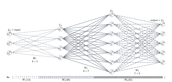
(a) Sample dense network

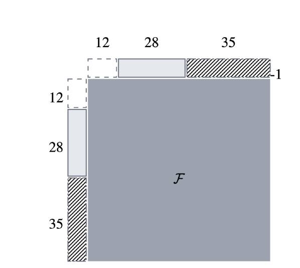
(b) Full FIM

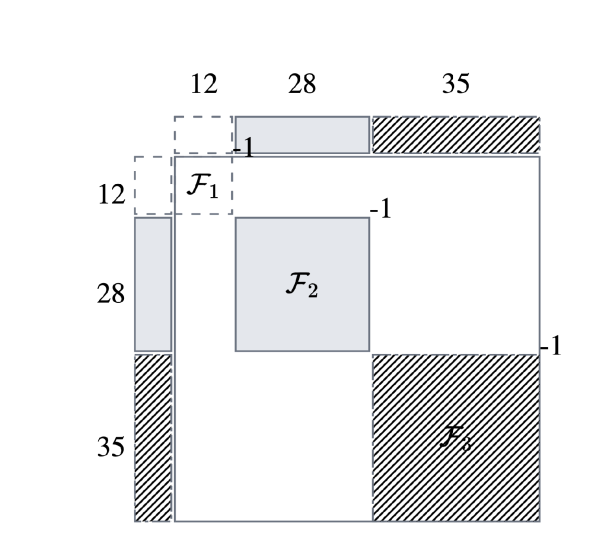
(c) Layer-Wise FIM

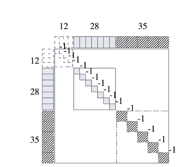
(d) CW-NGD: Component-Wise FIM

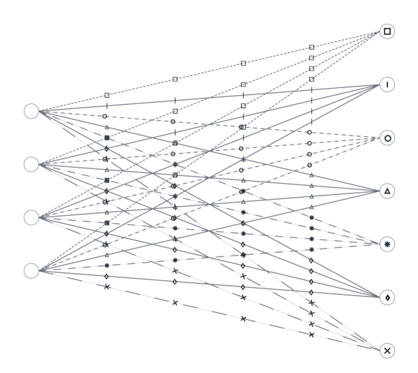
(e) Independent components

Figure 1: The approximation of a dense layer’s FIM and its inverse

III-C Approximate FIM Inverse for Dense Layer

For the sake of transparent interpretation, we consider a simple dense network illustrated in Figure 1(a). The original NGD algorithm requires inverting the FIM depicted in Figure 1(b). Figure 1(c) represents the Layer-Wise NGD algorithm family’s mechanism, where they approximate the FIM as a block-diagonal matrix and inverts each diagonal block. In CW-NGD, we divide the weight vector $\theta_{l}$ into groups in which elements of a group share the same output node (Figure 1(e)). Namely, we divide $\theta_{l}$ (or $\mathcal{D}_{\theta,l}$) into $n_{l}$ groups of elements $\theta_{l,:,i}$ (or $\mathcal{D}_{\theta,(l,:,i)}$) ($i=1,2,\ldots,n_{l}$). Thanks to the definition of the vectorization function $vec$ of the weight matrix, elements in the same group are consecutive in the vectorized presentation of the weight. This results in $\mathcal{F}_{\theta,l}$ being a $n_{l}$ by $n_{l}$ block matrix in which the $i$-th row and $j$-th block is $\mathcal{F}_{\theta,(l,:,i),(l,:,j)}$. By definition of $\mathcal{F}_{\theta}$ given in Eq. 1, we have:

$$\mathcal{F}_{\theta,(l,:,i),(l,:,j)} =\sum_{p=1}^{p=P}\left({\mathcal{D}_{\theta,(l,:,i)}^{(p)}}^{\intercal}\mathcal{D}_{\theta,(l,:,j)}^{(p)}\right)$$ (4)

There is a well-known assumption that holds very well in practice [32] called gradient independence assumption in the mean field theory. It is inspired by [33], first introduced in [34], and later applied in numerous studies in Deep Neural Networks [35, 36, 37, 32, 38, 39, 13]. Under this assumption, the network weight for backpropagation is assumed to be different from those used in forwarding propagation and identically independently sampled from the same distributions. That means their covariance is zero. For $i\neq j$, we have:

$$0 =cov(\mathcal{D}_{\theta,(l,:,i)},\mathcal{D}_{\theta,(l,:,j)})$$ (5)

$$0 =\mathbb{E}\left[\mathcal{D}_{\theta,(l,:,i)}^{\intercal}\mathcal{D}_{\theta,(l,:,j)}\right]-\mathbb{E}\left[\mathcal{D}_{\theta,(l,:,i)}\right]^{\intercal}\mathbb{E}\left[\mathcal{D}_{\theta,(l,:,j)}\right]$$ (6)

$$0 =\mathbb{E}\left[\mathcal{D}_{\theta,(l,:,i)}^{\intercal}\mathcal{D}_{\theta,(l,:,j)}\right]$$ (7)

The last equality is based on the zero expectation property of the score function [40] ($\mathbb{E}\left[\mathcal{D}_{\theta,(l,:,i)}\right]=0$) that satisfies under overwhelmingly the majority of the cases within the application of neural networks [41] and can be trivially proven using the Leibniz Integral Rule [42]. Evaluating the Eq. 7 with samples from dataset, we have $\sum_{p=1}^{p=P}\left({\mathcal{D}_{\theta,(l,:,i)}^{(p)}}^{\intercal}\mathcal{D}_{\theta,(l,:,j)}^{(p)}\right)=0$ for $i\neq j$. Correspondingly, off-diagonal blocks of layer FIM (Eq. 4) are zero. As a result, the dense layer’s FIM becomes a block-diagonal matrix whose inverse can be calculated by inverting its diagonal block sub-matrices within a reasonable time. Figure 1(d) reveals the mechanism of CW-NGD.

$$\mathcal{F}_{\theta,l}=diag(\mathcal{F}_{\theta,(l,:,1),(l,:,1)},\ldots,\mathcal{F}_{\theta,(l,:,n_{l}),(l,:,n_{l})})$$

$$\mathcal{F}_{\theta,l}^{-1}=diag(\mathcal{F}_{\theta,(l,:,1),(l,:,1)}^{-1},\ldots,\mathcal{F}_{\theta,(l,:,n_{l}),(l,:,n_{l})}^{-1})$$

In summary, in the CW-NGD method, we apply the derivative independence assumption to pairs of edges associated with different output nodes (Figure 1(e)). This division is based on the observation that elements across different groups do not directly contribute to the loss function at the $l$-th layer stage of the calculation in $f(x,\theta)$. To put it in another way, 2 elements belonging to 2 different groups contribute to different output nodes whose values are passed through the activation function before contributing to the same output node in the next layer. By the chaining rule which is used in backpropagation, the derivative with respect to the next layer’s output node must be multiplied with the derivative with respect to different output nodes in the current layer before being used to calculate the derivative with respect to these 2 elements. These analyses are further supported by our empirical result, which will be shown in Section V.

III-D Approximating the FIM for Convolutional Layers

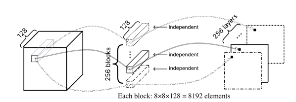
Figure 2: Sample CNN

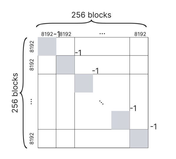
Figure 3: CW-NGD’s FIM’s approximation for CNN layers

This subsection focuses on approximating the FIM for convolutional layers. Figure 2 exposes the structure of a sample convolutional with filter size $8\times 8$, input layer having 128 channels, output layer having 256 channels. The array of blocks in the middle of Figure 2 represents the weight of the layer consisting of 256 blocks with each block having $8\times 8\times 128=8192$ scalar elements. Because convolutional layers have a different structure from dense layers, we need to adapt the notation accordingly. Most of the formulae are the same as of the dense layer case, though.

Suppose that between the $(l-1)$-th layer with $c_{l-1}$ channels and the $l$-th layer with $c_{l}$ channels, there is a 2D convolutional layer with a $k_{l}\times e_{l}$-size kernel. The convolutional layer has the weight tensor in a shape $k_{l}\times e_{l}\times c_{l-1}\times c_{l}$ and the bias in a shape $c_{l}$. Diverging from the case of dense layer, for the convolutional layer, we use the index notation $\theta_{l,r,h,i,o}$ (or $\mathcal{D}_{\theta,(l,r,h,i,o)}$) to refer to the element of the flattened vector $\theta$ (or $\mathcal{D}_{\theta}$) associated with the element of the weight of the $l$-th (convolutional) layer at $(r,h,i,o)$ index with $r,h$ being kernel’s indices and $i,o$ being input layer and output filter’s indices, respectively. For the bias element, we use the notations $\theta_{l,o}$ and $\mathcal{D}_{\theta,(l,o)}$ instead.

The associated layer FIM for this convolutional layer turns in a shape $(c_{l}+k_{l}e_{l}c_{l-1}c_{l})\times(c_{l}+k_{l}e_{l}c_{l-1}c_{l})$. We index this FIM using the notations $\mathcal{F}_{\theta,(l_{1},r_{1},h_{1},i_{1},o_{1}),(l_{2},r_{2},h_{2},i_{2},o_{2})}$, $\mathcal{F}_{\theta,(l_{1},r_{1},h_{1},i_{1},o_{1}),(l_{2},o_{2})}$, $\mathcal{F}_{\theta,(l_{1},o_{1}),(l_{2},r_{2},h_{2},i_{2},o_{2})}$, and $\mathcal{F}_{\theta,(l_{1},o_{1}),(l_{2},o_{2})}$ for respective pairs of element types described using the index notation for the weight tensor $\theta$.

The convolutional layer structure does not affect the generality of the derivative independence assumption and its derivation to the block-diagonal matrix approximation of the FIM described in Subsection III-C. All we need to do is to provide an appropriate grouping scheme for an efficient approximation. For the case of the dense layer, we divide the weight into groups by output node. In contrast, for the convolutional layer, we divide the weight and bias into groups by their output layers. In other words, $\mathcal{D}_{\theta,l}$ is divided into $c_{l}$ groups. For $o=1,2\cdots,c_{l}$, the $o$-th group contains 1 element of $\mathcal{D}_{\theta,(l,o)}$ and $k_{l}e_{l}c_{l-1}$ elements from $\mathcal{D}_{\theta,(l,:,:,:,o)}$. In the flattened representation of the weight tensor, we place the elements in each group consecutively, beginning with the bias element. Applying the derivative independence assumption, the FIM becomes a block-diagonal matrix consisting of $c_{l}$ blocks, each of which is a $(1+k_{l}e_{l}c_{l-1})\times(1+k_{l}e_{l}c_{l-1})$ matrix. In this form, the FIM can be inverted in a reasonable time. Figure 3 shows how the FIM and its inverse are approximated for the case of the sample convolutional layer.

The division strategy for the convolutional layer is designed in the same way as the dense layer case. In which elements belonging to different groups do not directly contribute to the forward propagation of the network at the same stage of the current layer. To put it another way, their values contribute to different output nodes whose values are passed through the activation function before contributing to the same output node in the next layer. Hence, in backpropagation, the derivative with respect to the next layer’s output node must be multiplied with the derivative of the activation function with respect to different output nodes in the current layer before being used to calculate the network loss’s derivative with respect to these 2 elements.

The mechanism of CW-NGD for convolutional layers clearly clarifies our contribution compared to the unit-wise NGD method [20, 24]. Unit-wise NGD coincides with CW-NGD in the case of dense layers. However, for convolutional layers, the layer has $W_{l}H_{l}c_{l}$ output nodes and many of them share the same weights, making unit-wise NGD impossible to group the weights by output nodes for update.

On the other hand, regarding the derivative independence assumption, it is theoretically possible to apply it to all pairs of different weight elements and yield FIM in form of a scalar diagonal matrix. [13] calls this method as entry-wise NGD, evaluates it on a crafted dataset and shows that it converges faster than the pure first-order methods (stochastic gradient descent), but slower than layer-wise NGD and unit-wise NGD. In our proposed method CW-NGD, we apply the derivative independence assumption to selected pairs of elements based on the grouping strategy which is designed based on the layer structure. Additionally, we empirically show that CW-NGD produces an efficient training convergence in a more practical dataset in Section V.

III-E Efficient CW-NGD Implementation and Discussion

Algorithm 1 Component-Wise Natural Gradient Descent

1:procedure CW-NGD($X\in\mathbb{R}^{P\times n_{0}}$, $Y\in\mathbb{R}^{P}$)

2:   $S,A\in\left[\mathbb{R}^{P\times n_{l}}\cup\mathbb{R}^{P\times r_{l}\times h_{l}\times c_{l}}\right]_{l=1,\ldots,L}\leftarrow$ ForwardProp($X$)

3:   $D_{a}\in\mathbb{R}^{P\times n_{L}}\cup\mathbb{R}^{P\times r_{L}\times h_{L}\times c_{L}}\leftarrow$ Cost^′($A_{[L]},Y$)

4:   delete $A_{[L]}$

5:   for $l$ from $L$ to 2 do

6:      $D_{s}\in\mathbb{R}^{P\times n_{l}}\cup\mathbb{R}^{P\times r_{l}\times h_{l}\times c_{l}}\leftarrow D_{a}\times act_{l}^{\prime}(S_{[l]})$

7:      $D_{a}\in\mathbb{R}^{P\times n_{l-1}}\cup\mathbb{R}^{P\times r_{l-1}\times h_{l-1}\times c_{l-1}}\leftarrow$ BackProp_l($D_{s}$)

8:      if layer_l is dense then

9:         $D_{W}\in\mathbb{R}^{P\times n_{l-1}\times n_{l}}\leftarrow A_{[l-1]}^{\intercal}\times D_{s}$

10:         $D_{W}^{\prime}\in\mathbb{R}^{n_{l}\times P\times n_{l-1}}\leftarrow$ Reshape($D_{W}$)

11:         $F\in\mathbb{R}^{n_{l}\times n_{l-1}\times n_{l-1}}\leftarrow D_{W}^{\prime\intercal}\times D_{W}^{\prime}$

12:         $D_{w}\in\mathbb{R}^{n_{l}\times n_{l-1}}\leftarrow$ Avg₁($D_{W}$)

13:         $D_{w}^{\prime}\in\mathbb{R}^{n_{l}\times 1\times n_{l-1}}\leftarrow$ Reshape($D_{w}$)

14:         $U^{\prime}\in\mathbb{R}^{n_{l}\times 1\times n_{l-1}}\leftarrow D_{w}^{\prime}\times\left(F+\gamma I\right)^{-1}$

15:         $U\in\mathbb{R}^{n_{l-1}\times n_{l}}\leftarrow$ Reshape($U^{\prime}$)

16:         $W_{l}\leftarrow W_{l}-\alpha U$

17:      else if layer_l is convolutional then

18:         $D_{W}\in\mathbb{R}^{P\times k_{l}\times e_{l}\times c_{l-1}\times c_{l}}\leftarrow$ Conv2DGrad($A_{[l-1]},D_{s}$)

19:         $D_{W}^{\prime}\in\mathbb{R}^{c_{l}\times P\times k_{l}e_{l}c_{l-1}}\leftarrow$ Reshape($D_{W}$)

20:         $F\in\mathbb{R}^{c_{l}\times k_{l}e_{l}c_{l-1}\times k_{l}e_{l}c_{l-1}}\leftarrow D_{W}^{\prime\intercal}\times D_{W}^{\prime}$

21:         $D_{w}\in\mathbb{R}^{k_{l}\times e_{l}\times c_{l-1}\times c_{l}}\leftarrow$ Avg₁($D_{W}$)

22:         $D_{w}^{\prime}\in\mathbb{R}^{c_{l}\times 1\times k_{l}e_{l}c_{l-1}}\leftarrow$ Reshape($D_{w}$)

23:         $U^{\prime}\in\mathbb{R}^{c_{l}\times 1\times k_{l}e_{l}c_{l-1}}\leftarrow D_{w}^{\prime}\times\left(F+\gamma I\right)^{-1}$

24:         $U\in\mathbb{R}^{k_{l}\times e_{l}\times c_{l-1}\times c_{l}}\leftarrow$ Reshape($U^{\prime}$)

25:         $W_{l}\leftarrow W_{l}-\alpha U$

26:      end if

27:      delete $A_{[l-1]},S_{[l]}$

28:   end for

29:end procedure

In this subsection, we provide an efficient implementation for CW-NGD. Next, we evaluate the computational complexity gained by the approximation in CW-NGD. Finally, we discuss the parallelization capabilities of CW-NGD with SIMD and MIMD.

Pseudocode of CW-NGD is described in Algorithm 1. CW-NGD takes two variables, inputs $X$ and labels $Y$, and updates the network weight with our proposed method. This procedure should be repeated multiple times, where the number of times is determined by the user. We drop the bias element for simplicity. In Algorithm 1, $P,\alpha,\gamma,I$ are batch size, scalar learning rate, scalar damping factor, and unit matrix of appropriate dimension, respectively. The notation $[]_{l=1,\ldots,L}$ denotes an array of $L$ element numbered by $l$ for example $S$ (or $A$), and $S_{[l]}$ (or $A_{[l]}$) refers to the $l$-th element of the array $S$ (or $A$). ForwardProp($X$) is the forward propagation of the network which returns $L$ elements arrays of pre-activation and (post-)activation evaluation of the network. The network might contain layers of other different types (MaxPooling, Flatten, etc.), but here we focus on and denote the 2 trainable types of dense ($\mathbb{R}^{P\times n_{l}}$) and convolutional ($\mathbb{R}^{P\times r_{l}\times h_{l}\times c_{l}}$) layers only. Cost^′($A_{[L]},Y$) is the derivative function of the cost function with respect to the last layer. The loop from Line 5 iterates from the last layer to the second layer, and carries out the backpropagation while inverting the FIM to precondition the gradient for updating the weights. In this for-loop, $act_{l}^{\prime}(S_{[l]})$ returns the Jacobian of the $l$-th layer’s activation function, BackProp_l($D_{s}$) is the backpropagation of the $l$-th layer which returns the derivative with respect to the previous layer (the $(n-1)$-th layer)’s (post-)activation. For matrix multiplication ($\times$), transpose(^⊺), and inversion(^-1) operations, when the operands are tensors of a dimension larger than 2, the operation is performed on the last two dimensions. For example, multiplying a $P\times N_{1}\times N_{2}$ tensor with a $P\times N_{2}\times N_{3}$ tensor results a $P\times N_{1}\times N_{3}$ tensor by aggregating results of $P$ multiplications of a $N_{1}\times N_{2}$ matrix with a $N_{2}\times N_{3}$ matrix. Avg₁($A$) is the average of the $A$ tensor along the first dimension. Reshape($A$) is the reshape function that re-arranges elements of the $A$ tensor into a tensor of a shape specified by the target shape on the left-hand side.

It is worth noting that the backpropagation (Line 7) calculates the derivative of the cost function with respect to each sample (post-)activation. This is different from the typical backpropagation in popular libraries that only supports calculating the sum of these derivatives. Besides, when taking the gradient (Line 12, Line 21), we use the average of the derivative with respect to the weight evaluated at each sample instead of the sum. The aggregation depends on how the loss across batch samples is aggregated. If the loss is averaged across samples, then the gradient should be averaged. Otherwise, when the loss is summed, the gradient should be summed as well. $\gamma$ is a scalar damping factor that is used (Line 14, Line 23) to prevent the FIM from becoming singular by decreasing its condition number. This technique is the well-known Tikhonov regularization [43] with the Tikhonov matrix being the identity matrix multiplied by $\gamma$. Tikhonov regularization is proven to be equivalent to imposing a sphere region called the trust region on the update vector [44]. So that, sometimes it is also called the trust region method. Tikhonov regularization is the first-to-use and very simple regularization method used in many quadratic curvature-related problems. In CW-NGD, we use a relatively small damping factor $\gamma$ and find it highly effective in making the FIMs invertible.

Next, we discuss the computational complexity gained by the approximation in CW-NGD and the memory complexity of the implementation. The computational complexity of CW-NGD is determined by the most expensive operation of inverting the FIM. In which, for each layer, we need to invert $n_{l}$ matrices of dimension $n_{l}\times n_{l}$ (dense) or invert $c_{l}$ matrices of dimension $k_{l}e_{l}c_{l-1}\times k_{l}e_{l}c_{l-1}$ (convolutional). Equivalently, the overall computation complexity is $\mathcal{O}(Ln_{l}^{4})+\mathcal{O}(Lk_{l}^{3}e_{l}^{3}c_{l}^{4})$, reduced $\mathcal{O}(max(L^{2}n_{l}^{2},L^{2}c_{l}^{2}))$ times from $\mathcal{O}(L^{3}n_{l}^{6})+\mathcal{O}(L^{3}k_{l}^{3}e_{l}^{3}c_{l}^{6})$ if we invert the full FIM.

From the memory perspective, we evaluate the individual FIM of each layer and update the layer’s weight during the backpropagation. We reuse many large-size variables such as $D_{W},D_{W}^{\prime},F,D_{w},D_{w}^{\prime},U^{\prime},U$, which efficiently reduces memory usage. Additionally, we remove the pre- and post-activations of each layer immediately after use (Line 4, Line 27).

Lastly, we discuss the parallelization capabilities of CW-NGD with SIMD and MIMD. The SIMD technique can be applied on various matrix operations, especially the FIM inversion (Line 14, Line 23). Moreover, the inverting operations of the FIM for individual layers and individual components are independent. So that they can be evaluated in parallel, and the computational complexity can be further scaled down to $Ln_{l}$ parallel processes for dense layer (or $Lc_{l}$ processes for convolutional layer) with each process’s computation complexity being $\mathcal{O}(n_{l}^{3})$ ($\mathcal{O}(k_{l}^{3}e_{l}^{3}c_{l}^{3})$ for convolutional layer).

Figure 4: Model used to train

IV Experiment

In this section, we describe the details of the conducted experiment including implementation framework, network architecture, dataset, training parameters, and the running environment.

To verify the effectiveness of our proposed method CW-NGD, we train the model described in Figure 4 on the MNIST dataset [27] using 3 different training methods: CW-NGD, KFAC [14, 15], and Adam [2]. The latter 2 methods are the state-of-the-art second-order and first-order optimization methods in the literature, respectively. The trained model starts with a convolutional layer and a max-pooling layer, followed by 2 dense layers. Kernel sizes, max pooling window size, and dense layer output sizes are all illustrated in Figure 4. Additionally, we use He Initialization [45] for all trainable weights.

Our implementation of CW-NGD is based on the latest TensorFlow [46] framework version 2.9.1. For Adam, we use the library call available in the framework. For KFAC, we use the implementation provided by Tensorflow team at [47] that requires Tensorflow version 1.15.

The experiment is conducted on the MNIST dataset [27] including 60,000 training samples and 10,000 testing samples, which are used to determine the training accuracy and validation accuracy described in Section V. We use the 1024 batch size and train the model in 100 epochs. In CW-NGD, we set learning rate $\alpha=1$ and damping factor $\gamma=0.0001$ according to Algorithm 1. For Adam, we use the parameter values and decay strategy provided in [47] tuned for the CIFAR10 dataset [48]: momentum $\beta=0.97$, learning rate: initialized at $2.24$ decaying to $0.0001$ at rate $0.9994$, epsilon: initialized at $0.183$ decaying to $10^{-8}$ at rate $0.9998$. Similarly, for KFAC, we use the parameter values and decay strategy provided in [47] tuned for the CIFAR10 dataset [48]: momentum $\beta=0.98$, learning rate: initialized at $0.23$ decaying to $0.0001$ at rate $0.9989$, damping factor: initialized at $0.289$ decaying to $10^{-6}$ at rate $0.9997$. Due to the resource constraint, we use the hyperparameter values tuned for CIFAR10 to use in this experiment which trains on the MNIST dataset for a heuristic comparison. This heuristic comparison is sufficient because the hyperparameters only affect the early iterations of the training.

Because the available KFAC implementation is implemented in the legacy Tensorflow version which requires a specific environment (CUDA 10.0, GCC 7.5.0), to simplify the experiment process, we run the experiment on 2 machines. One is equipped with a TITAN RTX GPU, and the other is equipped with a GTX 3080 GPU. The former is installed with Tensorflow version 2.9.1 (Python 3.10, CUDA 11.2, Cudnn 8.1, GCC 12.1.0) to evaluate CW-NGD and Adam, while the latter is installed with Tensorflow version 1.15 (Python 3.7, CUDA 10.0, Cudnn 7.4, GCC 7.5.0) to evaluate KFAC. In 2 machines, Tensorflow automatically selects and makes use of GPGPU for the training.

V Results

Optimization	CW-NGD	Adam	KFAC
[l]1st training iteration
training accuracy	87.97%	85.85%	90.32%
[l]2nd training iteration
training accuracy	98.03%	95.89%	95.68%
[l]Number of iterations
needed for convergence	13	49	38
training accuracy	100%	100%	100%
validation accuracy	98.96%	98.68%	98.32%

TABLE I: Comparison among 3 optimization methods

In this section, we discuss the experiment results of 3 optimization methods (CW-NGD, Adam, KFAC) based on the graphs shown in Figure 5, with several statistic results in Table I.

Figure 5(a) gives an overview of the training accuracy of the three optimization methods. The higher curve of CW-NGD indicates that it performs better than the other two methods by converging within fewer iterations. Specifically, CW-NGD converges at the 13th iteration, while the other two methods converge at the 49th and 38th iterations (Table I). In other words, CW-NGD requires nearly one-third fewer iterations to converge than the other two methods.

Additionally, in Figure 5(a), CW-NGD curve smoothly and monotonically rises without fluctuating. This result can be partially explained by the absence of decaying strategy in CW-NGD training. In contrast, the other two methods’ graphs fluctuate due to the involvement of decaying strategies. CW-NGD achieves a higher training accuracy than the other two methods even before the first fluctuation, implying that CW-NGD produces a higher precondition for the gradient update compared to the other two methods. Table I shows that CW-NGD starts with a lower training accuracy than KFAC, better than Adam, then immediately gets a better training accuracy than both from the second iteration.

Regarding the validation accuracy, Figure 5(b) clearly indicates that CW-NGD outperforms the other two methods. To be precise, CW-NGD’s final validation accuracy is 98.96% while the other two methods’ final validation accuracies are lower and are 98.68% and 98.32%, respectively (Table I). Moreover, CW-NGD’s validation accuracy curve fluctuates less than the other two methods suggesting that CW-NGD’s produced gradient update precondition is more stable than the other two methods.

(a) Training Accuracy

(b) Validation Accuracy

Figure 5: Accuracy comparison among 3 optimization methods (higher is better)

VI Conclusion

In this work, we propose a novel method, named Component-Wise Natural Gradient Descent (CW-NGD), for training neural networks. CW-NGD is a second-order optimization that works by approximating the Fisher Information Matrix (FIM) required during the training as a block-diagonal matrix. Each block matrix in the diagonal corresponds to the FIM of a group of network weights in a layer. We introduce grouping strategies for CW-NGD that efficiently works on dense and convolutional layers. Our investigations show that CW-NGD runs in a reasonable time while preserving the accuracy of the model at a high level.

We provide the detail of an efficient implementation of CW-NGD that generates the FIM, inverts it, and updates the weights while doing the backpropagation. The implementation also reduces memory usage by reusing several large-size variables.

In an experiment that compares the number of iterations required for training convergence, we show that CW-NGD outperforms KFAC and Adam, 2 state-of-the-art second-order and first-order optimization methods in the literature, respectively. Specifically, CW-NGD only requires one-third of the iterations required by KFAC or Adam to converge.

In another experiment, we compare the validation accuracy of the 3 methods. The results reveal that CW-NGD clearly has the highest validation accuracy.

From the performance perspective, theoretically, the matrix inversion of the FIM can be divided into independent subproblems corresponding to the individual FIM of a component, each of which can be solved by a single process. This indicates the potential for a high parallelization level of CW-NGD. In the future, we will investigate a distributed solution of CW-NGD. Additionally, we will also extend CW-NGD to support layers other than dense and convolution. Besides, we are going to evaluate CW-NGD on more sophisticated datasets such as CIFAR10 [48], CIFAR100 [48], ImageNet [49], etc.

References

- [1] K. He, X. Zhang, S. Ren, and J. Sun, “Identity mappings in deep residual networks,” in Computer Vision – ECCV 2016. Springer International Publishing, 2016.
- [2] D. P. Kingma and J. Ba, “Adam: A method for stochastic optimization,” in 3rd International Conference on Learning Representations, ICLR 2015, San Diego, CA, USA, May 7-9, 2015, Conference Track Proceedings, 2015.
- [3] K. S. Geoffrey Hinton, Ni@sh Srivastava. Neural networks for machine learning, overview of mini-batch gradient descent. [Online]. Available: http://www.cs.toronto.edu/ tijmen/csc321/slides/lecture_slides_lec6.pdf
- [4] M. D. Zeiler, “Adadelta: An adaptive learning rate method,” ArXiv, 2012.
- [5] J. Duchi, E. Hazan, and Y. Singer, “Adaptive subgradient methods for online learning and stochastic optimization,” J. Mach. Learn. Res., 2011.
- [6] I. Sutskever, J. Martens, G. Dahl, and G. Hinton, “On the importance of initialization and momentum in deep learning,” in Proceedings of the 30th International Conference on Machine Learning, 2013.
- [7] S. Li, D. Li, and Y. Zhang, “Incorporating nesterov’s momentum into distributed adaptive gradient method for online optimization,” in 2021 China Automation Congress (CAC), 2021.
- [8] S.-i. Amari, “Natural Gradient Works Efficiently in Learning,” Neural Computation, 1998.
- [9] L. LeCam, Asymptotic methods in statistical decision theory, ser. Springer series in statistics. New York, NY [u.a.]: Springer, 1986.
-
[10]
A. Bernacchia, M. Lengyel, and G. Hennequin, “Exact natural gradient in deep
linear networks and its application to the nonlinear case,” in
Advances in Neural Information Processing Systems, S. Bengio,
H. Wallach, H. Larochelle, K. Grauman, N. Cesa-Bianchi, and R. Garnett, Eds.,
vol. 31. Curran Associates, Inc.,
2018. [Online]. Available:
https://proceedings.neurips.cc/paper/2018/file/
7f018eb7b301a66658931cb8a93fd6e8-Paper.pdf -
[11]
G. Zhang, J. Martens, and R. B. Grosse, “Fast convergence of natural gradient
descent for over-parameterized neural networks,” in Advances in Neural
Information Processing Systems, H. Wallach, H. Larochelle, A. Beygelzimer,
F. d'Alché-Buc, E. Fox, and R. Garnett, Eds.,
vol. 32. Curran Associates, Inc.,
2019. [Online]. Available:
https://proceedings.neurips.cc/paper/2019/file/
1da546f25222c1ee710cf7e2f7a3ff0c-Paper.pdf - [12] T. Cai, R. Gao, J. Hou, S. Chen, D. Wang, D. He, Z. Zhang, and L. Wang, “Gram-gauss-newton method: Learning overparameterized neural networks for regression problems,” 2019. [Online]. Available: https://arxiv.org/abs/1905.11675
- [13] R. Karakida and K. Osawa, “Understanding approximate fisher information for fast convergence of natural gradient descent in wide neural networks,” in Proceedings of the 34th International Conference on Neural Information Processing Systems, 2020.
- [14] J. Martens and R. Grosse, “Optimizing neural networks with kronecker-factored approximate curvature,” in Proceedings of the 32nd International Conference on Machine Learning, ser. Proceedings of Machine Learning Research, F. Bach and D. Blei, Eds., vol. 37. Lille, France: PMLR, 07–09 Jul 2015, pp. 2408–2417. [Online]. Available: https://proceedings.mlr.press/v37/martens15.html
- [15] R. Grosse and J. Martens, “A kronecker-factored approximate fisher matrix for convolution layers,” in Proceedings of the 33rd International Conference on International Conference on Machine Learning - Volume 48, ser. ICML’16. JMLR.org, 2016, p. 573–582.
- [16] J. Ba, R. Grosse, and J. Martens, “Distributed second-order optimization using kronecker-factored approximations,” in International Conference on Learning Representations, 2017. [Online]. Available: https://openreview.net/forum?id=SkkTMpjex
- [17] J. Martens, J. Ba, and M. Johnson, “Kronecker-factored curvature approximations for recurrent neural networks,” in International Conference on Learning Representations, 2018. [Online]. Available: https://openreview.net/forum?id=HyMTkQZAb
- [18] T. Heskes, “On ”natural” learning and pruning in multilayered perceptrons,” Neural Computation, vol. 12, 01 2000.
- [19] T. Kurita, “Iterative weighted least squares algorithms for neural networks classifiers,” in Algorithmic Learning Theory, 1993.
- [20] Y. Ollivier, “Riemannian metrics for neural networks I: feedforward networks,” Information and Inference: A Journal of the IMA, 2015.
- [21] N. Schraudolph, “Fast curvature matrix-vector products for second-order gradient descent,” Neural computation, 2002.
- [22] F. Kunstner, P. Hennig, and L. Balles, “Limitations of the empirical fisher approximation for natural gradient descent,” in Advances in Neural Information Processing Systems, 2019.
-
[23]
N. Roux, P.-a. Manzagol, and Y. Bengio, “Topmoumoute online natural gradient
algorithm,” in Advances in Neural Information Processing Systems,
J. Platt, D. Koller, Y. Singer, and S. Roweis, Eds., vol. 20. Curran Associates, Inc., 2007. [Online]. Available:
https://proceedings.neurips.cc/paper/2007/file/
9f61408e3afb633e50cdf1b20de6f466-Paper.pdf - [24] S.-i. Amari, R. Karakida, and M. Oizumi, “Fisher information and natural gradient learning in random deep networks,” in Proceedings of the Twenty-Second International Conference on Artificial Intelligence and Statistics, 2019.
- [25] D. C. Liu and J. Nocedal, “On the limited memory bfgs method for large scale optimization,” Mathematical programming, 1989.
- [26] A. S. Berahas, J. Nocedal, and M. Takac, “A multi-batch l-bfgs method for machine learning,” in Advances in Neural Information Processing Systems, 2016.
- [27] Y. LeCun and C. Cortes, “MNIST handwritten digit database,” 2010. [Online]. Available: http://yann.lecun.com/exdb/mnist/
- [28] H. Park, S.-I. Amari, and K. Fukumizu, “Adaptive natural gradient learning algorithms for various stochastic models,” Neural Networks, 2000.
- [29] R. Karakida, S. Akaho, and S.-i. Amari, “Universal statistics of fisher information in deep neural networks: Mean field approach,” in Proceedings of the Twenty-Second International Conference on Artificial Intelligence and Statistics, ser. Proceedings of Machine Learning Research, K. Chaudhuri and M. Sugiyama, Eds., vol. 89. PMLR, 16–18 Apr 2019, pp. 1032–1041. [Online]. Available: https://proceedings.mlr.press/v89/karakida19a.html
- [30] J. Martens, “New insights and perspectives on the natural gradient method,” Journal of Machine Learning Research, 2020.
- [31] R. Pascanu and Y. Bengio, “Revisiting natural gradient for deep networks,” in In International Conference on Learning Representations, 2014.
- [32] G. Yang and S. S. Schoenholz, “Mean field residual networks: On the edge of chaos,” in Proceedings of the 31st International Conference on Neural Information Processing Systems, ser. NIPS’17. Red Hook, NY, USA: Curran Associates Inc., 2017, p. 2865–2873.
- [33] T. P. Lillicrap, D. Cownden, D. B. Tweed, and C. J. Akerman, “Random feedback weights support learning in deep neural networks,” ArXiv, vol. abs/1411.0247, 2014.
- [34] S. S. Schoenholz, J. Gilmer, S. Ganguli, and J. Sohl-Dickstein, “Deep information propagation,” arXiv preprint arXiv:1611.01232, 2016.
- [35] G. Yang, “Scaling limits of wide neural networks with weight sharing: Gaussian process behavior, gradient independence, and neural tangent kernel derivation,” CoRR, vol. abs/1902.04760, 2019. [Online]. Available: http://arxiv.org/abs/1902.04760
- [36] W. Huang, R. Y. D. Xu, W. Du, Y. Zeng, and Y. Zhao, “Mean field theory for deep dropout networks: digging up gradient backpropagation deeply,” 24th European Conference on Artificial Intelligence - ECAI 2020, 2020.
- [37] G. Yang and S. S. Schoenholz, “Deep mean field theory: Layerwise variance and width variation as methods to control gradient explosion,” in ICLR 2018, 2018.
- [38] L. Xiao, Y. Bahri, J. Sohl-Dickstein, S. Schoenholz, and J. Pennington, “Dynamical isometry and a mean field theory of cnns: How to train 10,000-layer vanilla convolutional neural networks,” 06 2018.
-
[39]
R. Karakida, S. Akaho, and S.-i. Amari, “The normalization method for
alleviating pathological sharpness in wide neural networks,” in
Advances in Neural Information Processing Systems, H. Wallach,
H. Larochelle, A. Beygelzimer, F. d'Alché-Buc, E. Fox,
and R. Garnett, Eds., vol. 32. Curran
Associates, Inc., 2019. [Online]. Available:
https://proceedings.neurips.cc/paper/2019/file/
9edda0fd4d983bf975935cfd492fd50b-Paper.pdf -
[40]
G. Enderlein, “Wilks, s. s.: Mathematical statistics. j. wiley and sons, new
york–london 1962; 644 s., 98 s,” Biometrische Zeitschrift, vol. 6,
no. 3, pp. 214–215, 1964. [Online]. Available:
https://onlinelibrary.wiley.com/doi/abs/10.1002/
bimj.19640060317 - [41] A. Rothman. Derivations of the fisher information. [Online]. Available: https://towardsdatascience.com/derivations-of-the-fisher-information-bc81c82f12f6
- [42] D. Williams, Probability with Martingales., ser. Cambridge mathematical textbooks. Cambridge University Press, 1991.
- [43] P. Kennedy, A Guide to Econometrics, 5th Edition, ser. MIT Press Books. The MIT Press, 2003, vol. 1, no. 026261183x. [Online]. Available: https://ideas.repec.org/b/mtp/titles/026261183x.html
- [44] J. Nocedal and S. J. Wright, Numerical Optimization, 2nd ed. New York, NY, USA: Springer, 2006.
- [45] K. He, X. Zhang, S. Ren, and J. Sun, “Delving deep into rectifiers: Surpassing human-level performance on imagenet classification,” in 2015 IEEE International Conference on Computer Vision (ICCV), 2015, pp. 1026–1034.
- [46] M. Abadi, A. Agarwal, P. Barham, E. Brevdo, Z. Chen, C. Citro, G. S. Corrado, A. Davis, J. Dean, M. Devin, S. Ghemawat, I. Goodfellow, A. Harp, G. Irving, M. Isard, Y. Jia, R. Jozefowicz, L. Kaiser, M. Kudlur, J. Levenberg, D. Mané, R. Monga, S. Moore, D. Murray, C. Olah, M. Schuster, J. Shlens, B. Steiner, I. Sutskever, K. Talwar, P. Tucker, V. Vanhoucke, V. Vasudevan, F. Viégas, O. Vinyals, P. Warden, M. Wattenberg, M. Wicke, Y. Yu, and X. Zheng, “TensorFlow: Large-scale machine learning on heterogeneous systems,” 2015, software available from tensorflow.org. [Online]. Available: https://www.tensorflow.org/
- [47] T. Team, “K-fac: Kronecker-factored approximate curvature,” https://github.com/tensorflow/kfac, 2022.
- [48] A. Krizhevsky, V. Nair, and G. Hinton, “Cifar-10 (canadian institute for advanced research).” [Online]. Available: http://www.cs.toronto.edu/ kriz/cifar.html
- [49] J. Deng, W. Dong, R. Socher, L.-J. Li, K. Li, and L. Fei-Fei, “Imagenet: A large-scale hierarchical image database,” in 2009 IEEE Conference on Computer Vision and Pattern Recognition, 2009.