Factors of Influence of the Overestimation Bias of Q-Learning

Abstract

We study whether the learning rate $\alpha$, the discount factor $\gamma$ and the reward signal $r$ have an influence on the overestimation bias of the Q-Learning algorithm. Our preliminary results in environments which are stochastic and that require the use of neural networks as function approximators, show that all three parameters influence overestimation significantly. By carefully tuning $\alpha$ and $\gamma$, and by using an exponential moving average of $r$ in Q-Learning’s temporal difference target, we show that the algorithm can learn value estimates that are more accurate than the ones of several other popular model-free methods that have addressed its overestimation bias in the past.

1 Introduction and Preliminaries

Reinforcement Learning (RL) is a machine learning paradigm that aims to train agents such that they can interact with an environment and maximize a numerical reward signal. While there exist numerous ways of learning from interaction, in model-free RL this is achieved by learning value functions that estimate how good it is for an agent to be in a certain state, or how good it is for the agent to take a certain action in a particular state (Sutton & Barto, 2018). The goodness/badness of state-action pairs is typically expressed in terms of expected future rewards: the higher the expected value of a state-action tuple, the better it is for the RL agent to perform a certain action in a given state. Estimating state-action values accurately is therefore key when it comes to model-free RL, as it is in fact the agent’s value functions that define its actions and, as a result, allow it to interact optimally with its environment.

To express such concepts more formally, let us define the RL setting as a Markov Decision Process (MDP) represented by the following tuple $(\mathcal{S},\mathcal{A},P,r,\gamma)$ (Puterman, 2014). Its components are a state space $\mathcal{S}$, an action space $\mathcal{A}$, a transition probability distribution $P$, that defines the probability for an agent to visit state $s$ given action $a$ at time step $t$, $p(s_{t+1}|s_{t},a_{t})$, a reward signal $r$, coming from the reward function $\Re(s_{t},a_{t},s_{t+1})$, and a discount factor $\gamma\in[0,1)$. The actions of the RL agent are selected based on its policy $\pi:\mathcal{S}\rightarrow\mathcal{A}$ that maps each state to an action. For every state $s\in\mathcal{S}$, under policy $\pi$ the agent’s state-value function $V^{\pi}:\mathcal{S}\rightarrow\mathds{R}$ is defined as:

$$V^{\pi}(s)=\mathds{E}\bigg{[}\sum_{k=0}^{\infty}\gamma^{k}r_{t+k}\bigg{|}s_{t}=s,\pi\bigg{]},$$ (1)

while its state-action value function $Q:\mathcal{S}\times\mathcal{A}\rightarrow\mathds{R}$ is defined as:

$$Q^{\pi}(s,a)=\mathds{E}\bigg{[}\sum_{k=0}^{\infty}\gamma^{k}r_{t+k}\bigg{|}s_{t}=s,a_{t}=a,\pi\bigg{]}.$$ (2)

The main goal for the agent is to find a policy $\pi^{*}$ that realizes the optimal expected return:

$$V^{*}(s)=\underset{\pi}{\max}\>V^{\pi}(s),\ \text{for all}\ s\in\mathcal{S}$$ (3)

and the optimal $Q$ value function:

$$Q^{*}(s,a)=\underset{\pi}{\max}\>Q^{\pi}(s,a)\ \text{for all}\ s\in\mathcal{S}\ \text{and}\ a\in\mathcal{A}.$$ (4)

Learning these value functions is a well-studied problem in RL (Szepesvári, 2010; Sutton & Barto, 2018), and several algorithms have been proposed to do so. The arguably most popular one is Q-Learning (Watkins & Dayan, 1992) which keeps track of an estimate of the optimal state-action value function $Q:\mathcal{S}\times\mathcal{A}\rightarrow\mathds{R}$ and given a RL trajectory $\langle s_{t},a_{t},r_{t},s_{t+1}\rangle$ updates $Q(s_{t},a_{t})$ with respect to the greedy target $r_{t}+\gamma\max_{a\in\mathcal{A}}Q(s_{t+1},a)$. Despite guaranteeing convergence to $Q^{*}(s,a)$ with probability $1$, Q-Learning is characterized by some biases that can prevent the agent from learning (Thrun & Schwartz, 1993; Van Hasselt, 2010; Lu et al., 2018).

1.1 The Overestimation Bias of Q-Learning

Among such biases, the arguably most studied one is its overestimation bias: due to the maximization operator in its Temporal Difference (TD) target $\max_{a\in\mathcal{A}}Q(s_{t+1},a)$, Q-Learning estimates the expected maximum value of a state, instead of its maximum expected value, an issue which as discussed by Van Hasselt (2011) dates back to research in order statistics (Clark, 1961). As a result, most recent work aimed to reduce Q-Learning’s overestimation bias by replacing its $\max$ operator: Maxmin Q-Learning (Lan et al., 2020) controls it by trying to reduce the estimated variance of the different state-action values; whereas Variation Resistant Q-Learning (Pentaliotis & Wiering, 2021) does so by keeping track of past state-action value estimates that can then be used when constructing the TD-target of the algorithm. On a similar note, Karimpanal et al. (2021) also define a novel TD-target which is a convex combination of a pessimistic and an optimistic term. A relatively older approach is that of Van Hasselt (2010) who introduced the double estimator approach where one estimator is used for choosing the maximizing action while the other is used for determining its value. This approach plays a central role in his Double Q-Learning algorithm as well as in the more recent Weighted Double Q-Learning (Zhang et al., 2017), Double Delayed Q-Learning (Abed-alguni & Ottom, 2018) and Self-Correcting Q-Learning algorithms (Zhu & Rigotti, 2021). The recent rise of Deep Reinforcement Learning has shown that the overestimation bias of Q-Learning plays an even more important role when model-free RL algorithms are combined with deep neural networks, which in turn has resulted in a large body of works that have studied this phenomenon outside the tabular RL setting (Van Hasselt et al., 2016; Fujimoto et al., 2018; Kim et al., 2019; Cini et al., 2020; Sabatelli et al., 2020; Peer et al., 2021).

2 Methods

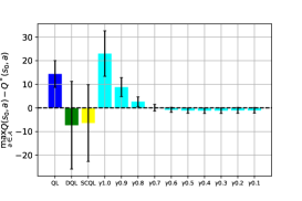
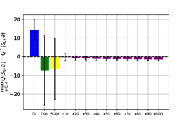
Figure 1: From left to right: our results showing that on the gridworld environment different values of $\alpha$, $\gamma$ and $x$ have an impact on the overestimation bias of Q-Learning. All factors of influence are compared against regular Q-Learning (blue), Double Q-Learning (green) and Self-Correcting Q-Learning (yellow).

While, as explained earlier, reducing Q-Learning’s overestimation bias has been mainly done by focusing on its $\max$ operator, in this paper, we take a different approach. Before introducing it, let us recall that Q-Learning learns $Q^{*}(s,a)$ as follows:

$$Q(s_{t},a_{t}):=Q(s_{t},a_{t})+\alpha\big{[}r_{t}+\gamma\>\underset{a\in\mathcal{A}}{\max}\>Q(s_{t+1},a)-\\ Q(s_{t},a_{t})\big{]}.$$ (5)

2.1 Factors of Influence

Instead of replacing the maximization estimator, we investigate whether overestimation can be prevented by tuning the following parameters:

1. The learning rate $\alpha$ also denoted as the step-size parameter, controls the extent to which a certain state-action tuple gets updated with respect to the TD-target. Typically, small values imply slow convergence, while larger values may lead to divergence (Pirotta et al., 2013). It is well known that Q-Learning’s maximization estimator enhances the divergence of the algorithm, therefore we investigate whether its overestimation can be controlled by adopting learning rates which are low and fixed instead of linearly or exponentially decaying as done by Van Hasselt (2010).

2. The discount factor $\gamma$ enables to control the trade-off between immediate and long term rewards. While for many years it was considered best practice to set $\gamma$ to a constant value as close as possible to $1$, more recent research has demonstrated that this might not always be the best approach (Van Seijen et al., 2019). In fact a constant value of $\gamma$ has proven to yield time-inconsistent behaviours (Lattimore & Hutter, 2014), failures in modelling agent’s preferences (Pitis, 2019) and sub-optimal exploration (François-Lavet et al., 2015). As mentioned by Fedus et al. (2019) there seems to be a growing tension between the original $\gamma$ formulation and current RL research, which, however, has not yet been studied from an overestimation bias perspective, a limitation which we start addressing in this work.

3. The reward signal $r_{t}$ causes overestimation in environments where rewards are stochastic. The larger the variance in stochastic rewards, the higher the potential for overoptimistic values to accumulate and propagate through the system. However, if one averages the reward observed for a certain state-action pair over time, these averaged values would deviate from the true mean with a smaller variance. Therefore, we examine if overestimation can be reduced by using an exponential moving average in Q-Learning’s TD-target which is computed as follows

   $$\hat{r}(s)\mathrel{+}=\frac{1}{x}(r(t)-\hat{r}(s)),$$ (6)

   where $x$ is a static hyperparameter determining the degree of weighting decrease.

2.2 Experimental Setup

We examine the effect on overestimation and performance of keeping $\alpha$ low and static, lowering $\gamma$, and using and averaged reward signal $\hat{r}$ instead of $r_{t}$ in three different environments, and compare the performance of Q-Learning (QL) to that of Double Q-Learning (Van Hasselt, 2010) (DQL) and Self-Correcting Q-Learning (Zhu & Rigotti, 2021) (SCQL). For the tabular setting, we use the Gridworld environment initially proposed by Van Hasselt (2010). The environment is a $3\times 3$ grid with stochastic rewards in non-terminal states of a Bernoulli distribution $r\in[-12,10]$ and a fixed reward of 5 in the terminal state. We also test the effect of $\alpha,\gamma$ and $\hat{r}$ on the OpenAI gym (Brockman et al., 2016) Blackjack-v0 environment, which simulates Blackjack including its stochastic state transitions and stochastic rewards. Lastly, we consider the function approximator case where we train a Deep-Q Network (Mnih et al., 2015) on the CartPole-v0 environment. In this environment, the value of the learning rate, and whether it is static or decaying, has already been shown to have a significant effect on overestimation (Chen et al., 2021). Our contribution here is examining the effect of the discount factor on overestimation. Note that, as rewards are deterministic, the method of replacing $r_{t}$ with $\hat{r}$ is not relevant here. We assess the impact of the aforementioned factors of influence by measuring the average gained reward obtained by the agent throughout training, as well as by quantifying the degree of overestimation by comparing $\max_{a\in\mathcal{A}}Q(s_{0},a)$ to $Q^{*}(s_{0},a)$. The latter is reported for all environments in Table 1 where we compute $\max_{a\in\mathcal{A}}Q(s_{0},a)-Q^{*}(s_{0},a)$: negative values mean that the tested algorithms suffer from underestimation bias, whereas positive values mean overestimation.

3 Results

Gridworld

In the Gridworld environment, the optimal policy is to reach the goal state in 4 steps. Considering the stochastic rewards $r\in[-12,10]$ in non-terminal states, the correct value for $\max_{a\in\mathcal{A}}Q(s_{0},a)$ under $\pi^{*}$ for $\gamma=0.95$ is $5\gamma^{4}+\sum_{k=0}^{3}(-1)\gamma^{k}\approx 0.36$ (see black line in the first plot of Fig.2). In the same figure we can see that QL trained with a dynamic $\alpha$ (blue line) produces an average estimate of $\approx 14.75$, therefore severely suffering from overestimation, whereas DQL and SCQL suffer from underestimation bias as they learn an estimate of $\approx-7.58$ and $-6.68$ respectively (see green and yellow lines). In Fig.1 we show what happens when experimenting with different values for $\alpha$ and $\gamma$ and, when computing $\hat{r}$ with different values of $x$. We can clearly see that all three parameters have a significant impact on Q-Learning’s overestimation bias. Different values of $\alpha$ and $x$ result in very minor overestimation and underestimation (first and third plots of Fig.1), whereas the lower the value of $\gamma$ (see second plot of Fig.1), the less Q-Learning overestimates. Note however that lower values of $\gamma$ might not always allow Q-Learning to learn the optimal policy. For our experiments we found that best results were obtained with setting $\gamma$ to $0.6$ (second plot of Fig.2). When it comes to $\alpha$ and $x$, Q-Learning estimates and performs best with $\alpha=0.05$ and $x=70$ (first and third plot of Fig.2). As mentioned earlier, all factors of influence reduce Q-learning’s overestimation bias, as summarized in Table 1, while also increasing the obtained reward significantly.

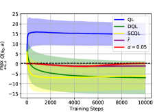
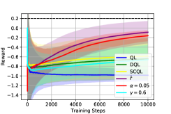
Figure 2: In clockwise order, our results showing that i) overestimation, as well as underestimation, can be prevented by using a constant value of $\alpha=0.05$ and by maintaining an exponential moving average estimate $\hat{r}$; ii) $\gamma=0.6$ allows Q-Learning to not overestimate; and iii) QL trained with either $\alpha=0.05$, $\gamma=0.6$ or $x=70$ outperforms regular QL, DQL and SCQL.

Blackjack

In Blackjack the optimal policy is known as basic strategy (Baldwin et al., 1956) and results in an average reward of $-0.045$. We determine the degree of overestimation of the different algorithms by setting $\gamma=1$ and by subtracting the average of the starting state Q values weighted by the occurrence, by the optimal performance. For this experiment we only consider $\gamma=1$ as the number of steps it takes to finish an episode and receive the reward is irrelevant to the strategy. We again observe that DQL and SCQL suffer from underestimation bias (see second row of Table 1) which, as shown by the reward plot in Fig.3, results in suboptimal performance. Because these algorithms underestimate state-action values, they tend to pursue a more defensive strategy that makes the agent stand its hand instead of drawing a new card.

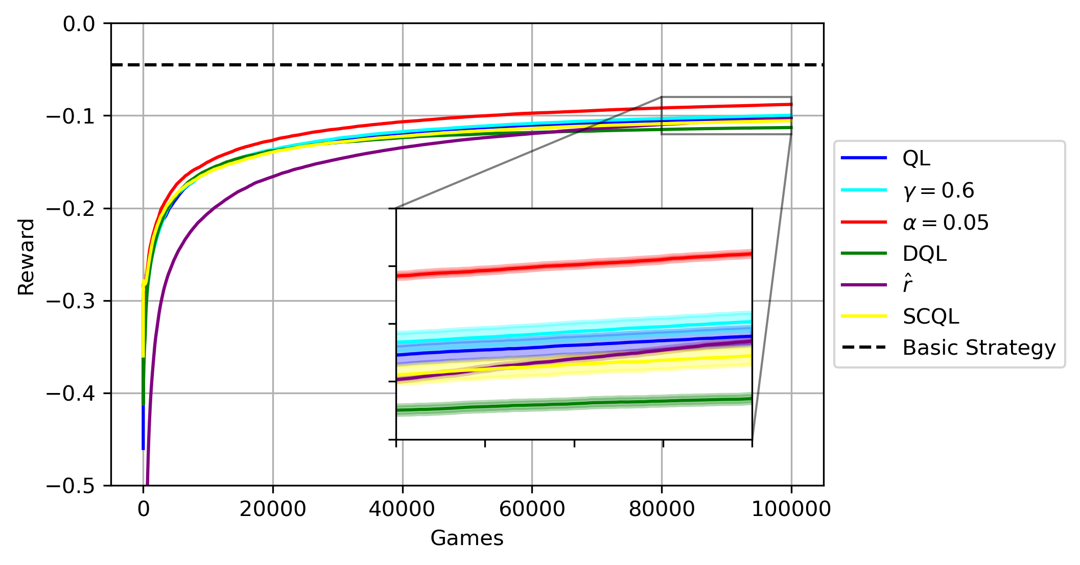
Figure 3: The rewards obtained by all algorithms on OpenAI’s Blackjack-v0 environment.

A static $\alpha$ and $\hat{r}$ slightly result in overestimation, which however does not prevent the algorithms from outperforming DQL and SCQL (see Fig.3). Surprisingly, also $\gamma=0.6$ results in better performance, however for this experiment we do not compute the degree of overestimation because of the complexity of the state space.

Deep Q-Learning

As there are multiple sources of stochasticity in neural networks, it is well known that Deep Q-learning suffers from overestimation even in fully deterministic environments (Van Hasselt et al., 2016). We investigate whether this could be prevented by lowering the discount factor. We find that on the Cartpole-v0 environment for $\gamma=0.999$, the algorithm performs well but estimations of the starting state (given $\gamma=0.999$ and a maximal cumulative reward of $200$ the optimal Q value is $\sum_{k}^{200}1\times\gamma^{k}\approx 181.35$) are highly varied and overly optimistic (see blue line of first plot of Fig.4). In the same plot we can also observe that Deep Double Q-Learning and Deep Self-Correcting Q-Learning suffer from the same underestimation bias that we already observed in the Gridworld environment (yellow and green lines). However, simply setting $\gamma=0.97$ improves the estimation significantly (second plot of Fig.4) without being detrimental to the overall performance of the algorithm (see third plot of Fig.4) which performs on par with a DQN, DDQN and SCQL agent trained with $\gamma=0.999$.

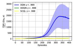
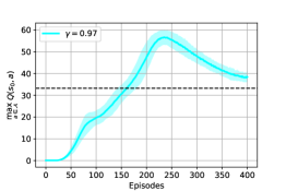
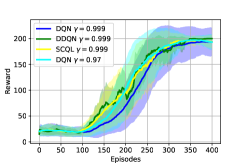
Figure 4: In clockwise order the results showing that: i) DQN suffers from severe overestimation when compared to DDQN and SCQL; ii) training a DQN agent with $\gamma=0.97$ mitigates this overestimation bias significantly; iii) a DQN agent trained with $\gamma=0.97$ performs just as well as all other algorithms trained with $\gamma=0.999$.

Table 1: Our results assessing the degree of overestimation of the different algorithms for all tested environments. We report $\max_{a\in\mathcal{A}}Q(s_{0},a)-Q^{*}(s_{0},a)$ where values $<0$ mean that the algorithms suffer from underestimation bias whereas values $>0$ mean overestimation.

	QL	DQL	SCQL	$\alpha$	$\gamma$	$\hat{r}$
Gridworld	+14.43	-7.22	-6.36	+0.095	+1.25	-1.42
Blackjack	+0.008	-0.080	-0.001	+0.026	-	+0.031
Cartpole	+1459.3	-131.9	-132.3	-	+3.47	-

4 Summary

We have studied the role of the learning rate $\alpha$, the discount factor $\gamma$ and the reward signal $r$ under the lens of the overestimation bias that characterizes the popular Q-Learning algorithm. Our results suggest that all three factors of influence play a significant role in Q-Learning’s estimations. As a result, we have provided initial intuition on how to set such parameters in order to prevent overestimation from happening in the tabular setting as well as in the function approximator one. We believe that stochasticity is among the core problems which causes Q-Learning’s $\max$ operator to overestimate, however, if one can work around the impact of stochasticity, as we tried with our methods, one can reduce overestimation without changing the maximization operator. By considering $\alpha,\gamma$ and $\hat{r}$ one can prevent overestimation in an easy, computationally not-intensive way as, differently from methods such as Double Q-Learning and Self-Correcting Q-Learning, there is no need to keep track of a second state-action table. Opportunities for future research are testing the methods on more environments, investigating the effects of an annealing exponential moving average value, and further investigating the applicability of our methods in the Deep Reinforcement Learning regime. Our goal there is to study the effects of $\alpha,\gamma$ and $\hat{r}$ with respect to the Deadly Triad of Deep Reinforcement Learning (Van Hasselt et al., 2018) and potentially construct a version of the DQN algorithm that does not require the use of a target network.

5 Appendix

For the function approximator case we replicate the network architecture and hyperparameters from Chen et al. (2021). Agents are trained for 400 episodes. The exploration strategy is epsilon greedy with an epsilon value that decreases linearly from 1.0 to 0.0. The network is an MLP with a first hidden layer of 48 units and second hidden layer of 96 units. The batch size is 512, and the target network is updated every 64 steps. Adam is used as an optimizer with standard values of $\beta_{1}=0.9$ and $\beta_{2}=0.999$. The learning rate is 0.0001.

All code to replicate the results is available at: https://github.com/overestimationbias/Factors-of-Influence-of-the-Overestimation-Bias

References

- Abed-alguni & Ottom (2018) Abed-alguni, B. H. and Ottom, M. A. Double delayed q-learning. International Journal of Artificial Intelligence, 16(2):41–59, 2018.
- Baldwin et al. (1956) Baldwin, R. R., Cantey, W. E., Maisel, H., and McDermott, J. P. The optimum strategy in blackjack. Journal of the American Statistical Association, 51(275):429–439, 1956.
- Brockman et al. (2016) Brockman, G., Cheung, V., Pettersson, L., Schneider, J., Schulman, J., Tang, J., and Zaremba, W. Openai gym. arXiv preprint arXiv:1606.01540, 2016.
- Chen et al. (2021) Chen, Y., Schomaker, L., and Wiering, M. A. An investigation into the effect of the learning rate on overestimation bias of connectionist q-learning. In ICAART (2), pp. 107–118, 2021.
- Cini et al. (2020) Cini, A., D’Eramo, C., Peters, J., and Alippi, C. Deep reinforcement learning with weighted q-learning. arXiv preprint arXiv:2003.09280, 2020.
- Clark (1961) Clark, C. E. The greatest of a finite set of random variables. Operations Research, 9(2):145–162, 1961.
- Fedus et al. (2019) Fedus, W., Gelada, C., Bengio, Y., Bellemare, M. G., and Larochelle, H. Hyperbolic discounting and learning over multiple horizons. arXiv preprint arXiv:1902.06865, 2019.
- François-Lavet et al. (2015) François-Lavet, V., Fonteneau, R., and Ernst, D. How to discount deep reinforcement learning: Towards new dynamic strategies. arXiv preprint arXiv:1512.02011, 2015.
- Fujimoto et al. (2018) Fujimoto, S., Hoof, H., and Meger, D. Addressing function approximation error in actor-critic methods. In International conference on machine learning, pp. 1587–1596. PMLR, 2018.
- Karimpanal et al. (2021) Karimpanal, T. G., Le, H., Abdolshah, M., Rana, S., Gupta, S., Tran, T., and Venkatesh, S. Balanced q-learning: Combining the influence of optimistic and pessimistic targets. arXiv preprint arXiv:2111.02787, 2021.
- Kim et al. (2019) Kim, S., Asadi, K., Littman, M., and Konidaris, G. Deepmellow: removing the need for a target network in deep q-learning. In Proceedings of the Twenty Eighth International Joint Conference on Artificial Intelligence, 2019.
- Lan et al. (2020) Lan, Q., Pan, Y., Fyshe, A., and White, M. Maxmin q-learning: Controlling the estimation bias of q-learning. arXiv preprint arXiv:2002.06487, 2020.
- Lattimore & Hutter (2014) Lattimore, T. and Hutter, M. General time consistent discounting. Theoretical Computer Science, 519:140–154, 2014.
- Lu et al. (2018) Lu, T., Schuurmans, D., and Boutilier, C. Non-delusional q-learning and value-iteration. Advances in neural information processing systems, 31, 2018.
- Mnih et al. (2015) Mnih, V., Kavukcuoglu, K., Silver, D., Rusu, A. A., Veness, J., Bellemare, M. G., Graves, A., Riedmiller, M., Fidjeland, A. K., Ostrovski, G., et al. Human-level control through deep reinforcement learning. nature, 518(7540):529–533, 2015.
- Peer et al. (2021) Peer, O., Tessler, C., Merlis, N., and Meir, R. Ensemble bootstrapping for q-learning. In International Conference on Machine Learning, pp. 8454–8463. PMLR, 2021.
- Pentaliotis & Wiering (2021) Pentaliotis, A. and Wiering, M. A. Variation-resistant q-learning: Controlling and utilizing estimation bias in reinforcement learning for better performance. 2021.
- Pirotta et al. (2013) Pirotta, M., Restelli, M., and Bascetta, L. Adaptive step-size for policy gradient methods. Advances in Neural Information Processing Systems, 26, 2013.
- Pitis (2019) Pitis, S. Rethinking the discount factor in reinforcement learning: A decision theoretic approach. In Proceedings of the AAAI Conference on Artificial Intelligence, volume 33, pp. 7949–7956, 2019.
- Puterman (2014) Puterman, M. L. Markov decision processes: discrete stochastic dynamic programming. John Wiley & Sons, 2014.
- Sabatelli et al. (2020) Sabatelli, M., Louppe, G., Geurts, P., and Wiering, M. A. The deep quality-value family of deep reinforcement learning algorithms. In 2020 International Joint Conference on Neural Networks (IJCNN), pp. 1–8. IEEE, 2020.
- Sutton & Barto (2018) Sutton, R. S. and Barto, A. G. Reinforcement learning: An introduction. 2018.
- Szepesvári (2010) Szepesvári, C. Algorithms for reinforcement learning. Synthesis lectures on artificial intelligence and machine learning, 4(1):1–103, 2010.
- Thrun & Schwartz (1993) Thrun, S. and Schwartz, A. Issues in using function approximation for reinforcement learning. In Proceedings of the 1993 Connectionist Models Summer School Hillsdale, NJ. Lawrence Erlbaum, volume 6, 1993.
- Van Hasselt (2010) Van Hasselt, H. Double q-learning. In Advances in neural information processing systems, pp. 2613–2621, 2010.
- Van Hasselt et al. (2016) Van Hasselt, H., Guez, A., and Silver, D. Deep reinforcement learning with double q-learning. In Proceedings of the AAAI conference on artificial intelligence, volume 30, 2016.
- Van Hasselt et al. (2018) Van Hasselt, H., Doron, Y., Strub, F., Hessel, M., Sonnerat, N., and Modayil, J. Deep reinforcement learning and the deadly triad. arXiv preprint arXiv:1812.02648, 2018.
- Van Hasselt (2011) Van Hasselt, H. P. Insights in reinforcement rearning: formal analysis and empirical evaluation of temporal-difference learning algorithms. PhD thesis, University Utrecht, 2011.
- Van Seijen et al. (2019) Van Seijen, H., Fatemi, M., and Tavakoli, A. Using a logarithmic mapping to enable lower discount factors in reinforcement learning. Advances in Neural Information Processing Systems, 32, 2019.
- Watkins & Dayan (1992) Watkins, C. J. and Dayan, P. Q-learning. Machine learning, 8(3-4):279–292, 1992.
- Zhang et al. (2017) Zhang, Z., Pan, Z., and Kochenderfer, M. J. Weighted double q-learning. In IJCAI, pp. 3455–3461, 2017.
- Zhu & Rigotti (2021) Zhu, R. and Rigotti, M. Self-correcting q-learning. In Proceedings of the AAAI Conference on Artificial Intelligence, volume 35, pp. 11185–11192, 2021.