Digital twins for city simulation: Automatic, efficient, and robust mesh generation for large-scale city modeling and simulation

Abstract

The concept of creating digital twins, connected digital models of physical systems, is gaining increasing attention for modeling and simulation of whole cities. The basis for building a digital twin of a city is the generation of a 3D city model, often represented as a mesh. Creating and updating such models is a tedious process that requires manual work and considerable effort, especially in the modeling of building geometries. In the current paper, we present a novel algorithm and implementation for automatic, efficient, and robust mesh generation for large-scale city modeling and simulation. The algorithm relies on standard, publicly available data, in particular 2D cadastral maps (building footprints) and 3D point clouds obtained from aerial scanning. The algorithm generates LoD1.2 city models in the form of both triangular surface meshes, suitable for visualisation, and high-quality tetrahedral volume meshes, suitable for simulation. Our tests demonstrate good performance and scaling and indicate good avenues for further optimization based on parallelisation. The long-term goal is a generic digital twin of cities volume mesh generator that provides (nearly) real-time mesh manipulation in LoD2.x.

1 Introduction

1.1 Digital twins and 3D city models

The need for creating digital replicas of physical systems has been around for decades [1] and the term twin was introduced already by NASA’s Apollo program [2]. In tandem, the term Digital Twin (DT) has been attracting significant attention in the last few years, especially in the context of the urban environment [1]. Behind the contemporary term lies mostly what software engineers refer to as plain old data, derived from multiple sources, stitched together in various forms and ready for consumption for different needs of the end-users of the twin. On the city scale, since the DT is required to serve a variety of purposes, including multi-physics simulations [3, 4], what-if scenarios [5, 6] and life-cycle analysis [7, 8], a common groundwork for the different means of the consumption of data is of great importance; even if the digital twin needs to adapt to which data is being analysed, the common denominator is a 3D city model [9].

3D city models generally enclose buildings and other built objects (road networks, green areas etc.). Often the process of 3D model creation is a manual or semi-manual process that is both tedious, time-consuming, and error-prone. Moreover, man-made city models tend to become outdated since their creation is a one-time project. Hence, creating and maintaining DTs is a challenging task [10, 11, 12, 13, 14]. The desired outcome is an automatically generated detailed 3D city model, or even multiple 3D models serving various analysis needs and purposes. The input to the process can be aerial imagery, topographic data, 3D LiDAR data, or a fusion of them. This 3D-fication process is a multi-step procedure and depending on the available input data and methods used, the quality of the outcome may vary greatly. For a complete, end-to-end solution, the pipeline involves developing robust systems for building detection, rooftop recognition, geometry modeling, and, eventually, mesh generation.

1.2 Contribution of this work

In the present work, we tackle the problem of creating LoD1.2 [15] 3D models of any urban environment in the form of both triangular surface meshes and tetrahedral volume meshes. The mesh generation is based on publicly available datasets from the Swedish Mapping, Cadastral and Land Registration Authority (https://www.lantmateriet.se) or any other similar repository that adheres to the same standards.

Our mesh generation strategy is unique in that it generates not only triangulated surfaces but also conforming tetrahedral volume meshes, suitable for high-performance simulations of, e.g., urban wind comfort and air quality by computational fluid dynamics (CFD). Such simulations require the 3D model generation to not only provide a surface model but also a high-quality computational volume mesh that is watertight, conforming, and satisfies a certain minimal angle condition.

The long-term goal is the creation of an automated process by which the computational mesh is generated as part of an interactive simulation environment. The demand for interactivity implies that the mesh generation be both efficient, i.e., the mesh generation should require minimal time as part of a simulation pipeline, and robust, i.e., the mesh generation pipeline should never break down as a result of bad or unexpected input data. The algorithms and software presented in the present work partially solve these goals and avenues for future optimisations are discussed to reach the long-term goal of (near) real-time generation of 3D models and meshes.

Our implementation DTCC Builder [16] is part of the Digital Twin Platform developed at the Digital Twin Cities Centre (https://dtcc.chalmers.se) and is available as free/open-source software (under the permissive MIT license).

1.3 Related work

The topic of automated creation of 3D city models from raw input data has received increasing attention in recent years [17], and there are many examples of 3D city models being created for specific consumption. For example in [18], a 3D model of the Beytepe Campus of Hacettepe University was generated and visualized using both Cesium and Potree JavaScript libraries. The authors initially used stereo photographs from an airplane which helped them generate a dense point cloud. Then, the point cloud was converted to a Digital Surface Model (DSM). The DSM was complemented by manually generating 106 building footprints from the stereo images. Finally, the DSM was combined with the building footprints in order to generate 3D building geometries in LoD1.2.

In [19], a 3D model of the city of Duisburg in the year 1566 was generated. To generate the 3D model of the city in that particular year, the authors used close-range terrestrial laser scanning on a wooden model of the city that exists in a cultural historic museum. The point cloud created by the scanning was combined with ortho-images of the wooden model to create 3D models of the buildings. Another example using LiDAR data is presented in [20] for analysis of the solar potential of building roofs in an urban 3D model.

In the same spirit, Lindberg et al. [21] present a model for estimating shortwave irradiance on ground, roofs and building walls. To showcase the results, the authors generated a 3D visualisation of an area in Gothenburg, Sweden. The ground and building DSMs were derived using geodata; two sets of data were used to derive the DSM, one LiDAR dataset for the ground heights and one high level of detail 3D vector layer describing the roof structures. Additional LiDAR datasets were used to generate a canopy DSM representing the height of bushes and/or trees and then the authors used the OpenGL library in R to showcase the results. Jian and Fan [22] present a simulation of harmful gas diffusion in 3D environment of an urban area. The authors performed their simulations in a generated model provided by Digital Earth Scientific Platform [23].

Striving to provide a more generic approach, the authors of [24] present a workflow for generating 3D models for any city. The researchers created a 3D city model in LoD1 for a part of the city of Ahmedabad in India. Initially, the contributors created DEMs using photogrammetry from satellite stereo images. Then, Automatic Terrain Extraction (ATE) was used to automatically extract DTMs from the generated DEMs. To automatically extract building footprints from high resolution satellite imagery, the authors used a combination of commercial software, Arc GIS and eCognition. In [25], a novel validated method for GIS based automated dynamic urban building energy simulations is presented. The authors visualize the city of Gleisdorf in 3D to highlight power consumption of all buildings. GIS data were collected to visualize the 2D building geometry. Then, a 2.5D geometry was generated from the 2D geometry and the height of the laser scanning for each building. Afterwards, building heights were assigned to each building directly in QGIS.

In [26], a different approach is used whereby the 3D city model is created from a Building Information Model (BIM) [27]. The authors present a workflow going from BIM to a 3D city model, but rely on the input data being handmade Industry Foundation Classes (IFCs). The authors conclude that the process is both time consuming and resource expensive, emphasizing the complexity of 3D city model creation. Alomia et al. [28] present the integration of procedural modeling and GIS for the development of a 3D city model. The workflow consists of geographic data capture of the area of interest on which building footprints are identified. Then, a mesh extrusion takes places to generate LoD1 buildings.

In [29], a technique for upgrading large-scale 2D GIS landscape representations into schematic 3D models is presented. The workflow uses a readily available 2D vector model along with elevation data. Geometric objects are generated from geo-processing tools and footprint shape extrusion results in LoD1 buildings. Additionally, the authors enriched the resulting model with some LoD2 assets that were modeled and photo-textured. In [30] a system that is capable of integrating, analysing and visualising 3D point clouds is presented. The implementation also provides pre-processing and analysis features to perform object class segmentation. In [31], a workflow to create a landscape model and 3D buildings based on old maps, plans, drawings and photographs is presented. The authors combined GIS techniques, 3D CAD software and procedural modelling tools.

In 2021, Ledoux et al. released open-source software [11, 14] that allows the automated 3D reconstruction of city models by using 2D topographical datasets which elevates them to the height obtained by point clouds. The end result is, according to the developers, “…surface(s) that aim(s) to be error-free: no self-intersections, no gaps, etc”. The same group very recently extended their work and released a new piece of open-source software City4CFD [32]. The code reconstructs terrain, buildings and surface layers (including water, roads, and vegetation) by combining 2D geographical datasets and LiDAR elevation data. The resulting geometry is then used as input to an external unstructured finite volume mesh generator and is used for CFD simulations using the OpenFOAM package [33]. The end-goal of these contributions is creating 3D models that can be used for more advanced analysis and simulation and not only for visualisation. This goal is shared by the present work.

1.4 Outline of this paper

In the remainder of this paper, we first present the results of our work on an automated process for efficient and robust 3D city model generation. The results consist of an overview of the algorithm and software, followed by a benchmark study on both synthetic and real-world data. We next discuss the performance and limitations of the algoritm and software based on the results the benchmark study. We then move on to presenting in some detail the algorithm for 3D city model generation, consisting of a pipeline of preprocessing and mesh generation steps. Finally, we comment on the implementation and how to obtain the software.

2 Results

2.1 Overview of algorithm and software

The starting point for our mesh generation pipeline is a cadastral map, i.e., a set of 2D polygonal building footprints, and a corresponding 3D point cloud, i.e., a set of 3D points. The cadastral map is assumed to be given in the standard shapefile (.shp) format and the point cloud is assumed to be given in the standard LAS (.las or .laz) format. Such data are readily available for most cities and in particular for the whole of Sweden from the Swedish Mapping, Cadastral and Land Registration Authority where we have sourced our data.

Given these two datasets, in combination with a 3D bounding box, our algorithm generates a tetrahedral mesh of the volume defined by the intersection of the bounding box and the empty space above and between the buildings and the ground. From the tetrahedral volume mesh, we also extract a triangular surface mesh by computing the boundary of the tetrahedral volume mesh. This mesh is automatically watertight and boundary conforming in the sense that the triangles on building surfaces necessarily align with the triangle surface (TIN) representing the ground.

In Figure 1, we demonstrate our algorithm for a pair of demo datasets. The first dataset named Majorna is a $2.5\text{\,}\mathrm{km}$ $\times$ $2.5\text{\,}\mathrm{km}$ large area in central Gothenburg, Sweden. This dataset is publicly available from the Swedish Mapping, Cadastral and Land Registration Authority. The dataset is also available as part of the distribution of our software [16]. The second dataset is a synthetically generated (randomized) city model which allows the building density to be controlled via a parameter. The figure shows the end result of the mesh generation pipeline as triangular surface meshes obtained by extracting the boundary of the generated tetrahedral volume meshes. Note that we show the surface meshes rather than the volume meshes since the surface meshes are more readily visualised.

Our mesh generation algorithm relies on two key ideas. First, the mesh generation is reduced from a 3D problem to a 2D problem by taking advantage of the cylindrical geometry of extruded 2D footprints; a 2D mesh respecting the boundaries of the buildings is generated by a 2D mesh generator and then layered to form a 3D mesh. Second, the 3D mesh is adapted to the geometries of building and ground by solving a partial differential equation (PDE) with the ground and building heights as boundary conditions (mesh smoothing). Together these two ideas enable the creation of a both efficient and robust pipeline for automated large-scale mesh generation from raw data. Our algorithm is described in detail in the Methods section of our paper.

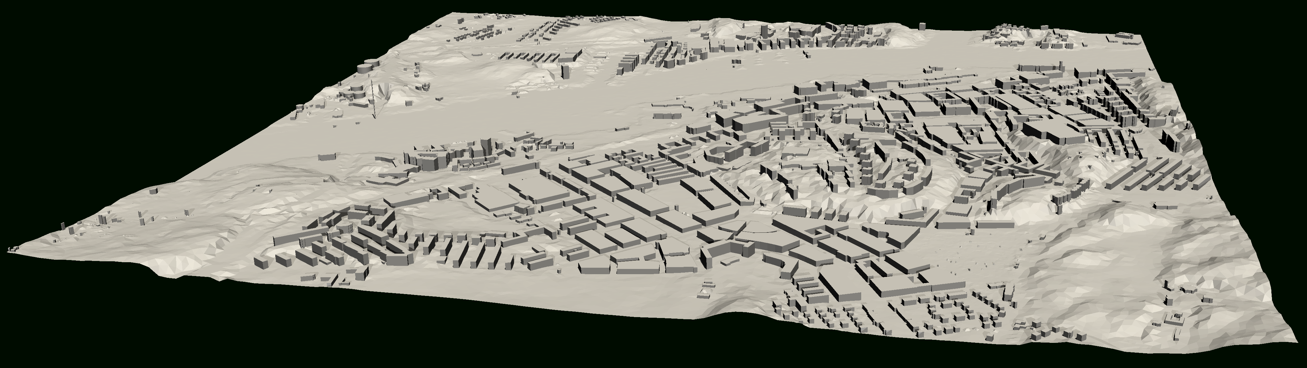
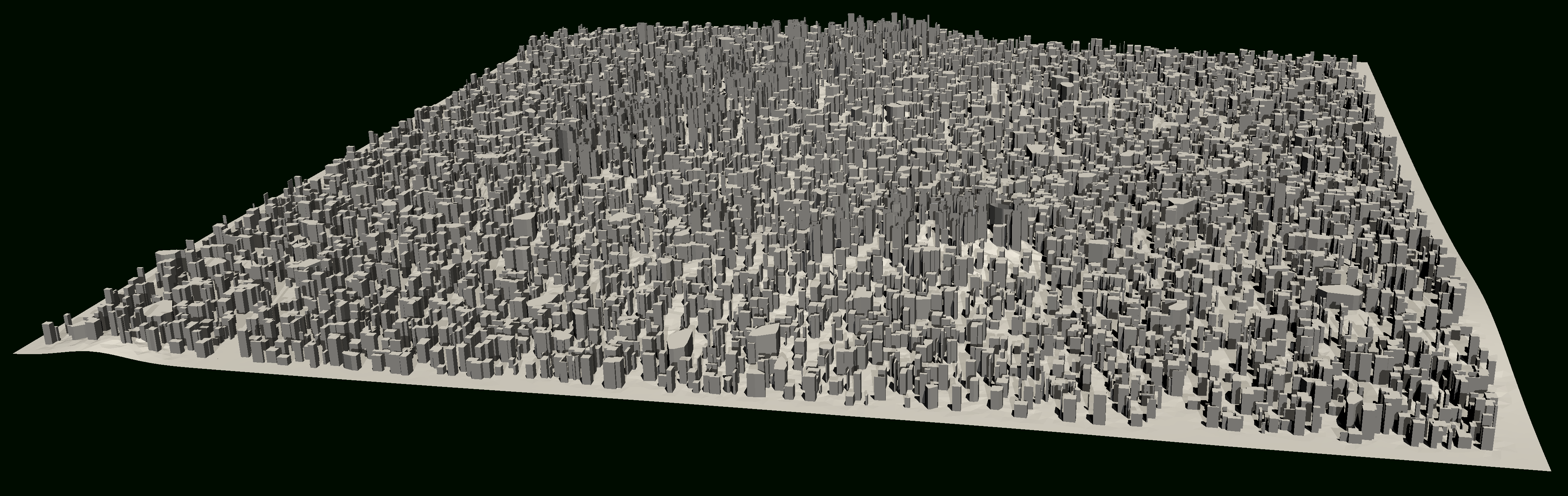
Figure 1: Top: Surface mesh of Majorna in Gothenburg Sweden. The city model consists of $3096$ buildings. Bottom: Surface mesh of a synthetic city model with $11\,585$ randomly placed buildings. Both models cover an area of size $2.5\text{\,}\mathrm{km}$ $\times$ $2.5\text{\,}\mathrm{km}$.

2.2 Benchmark study

To evaluate the efficiency and detect possible bottlenecks of our mesh generation pipeline, we conduct a benchmark study consisting of two different experiments. We investigate (a) how the computational cost scales with the mesh resolution (number of cells generated) and (b) how the computational cost scales with the number of buildings for a fixed area. For (a), we use a public dataset bundle from the Swedish Mapping, Cadastral and Land Registration Authority of an area located in Central Gothenburg, Sweden, a district called Majorna. For (b), we create a synthetic city, by placing $N$ randomly positioned buildings on a square tile the same size as the Majorna test case. Both configurations span the same area of $6.25\text{\,}\mathrm{k}\mathrm{m}^{2}$.

All benchmark cases were run on the same compute node powered by a Xeon^® Silver 4110 CPU @ 2.10GHz using a single thread. The maximum memory footprint was approximately 64 GB and 2 GB for the Majorna and synthetic city datasets, respectively.

The results of the benchmarks study are summarised in Figure 2 and Figure 3. The different steps (2.1–3.5) refer to the steps in our mesh generation pipeline described in the Methods section. We only measure the cost of steps 2.x and 3.x since steps 1.x consist of initial preprocessing.

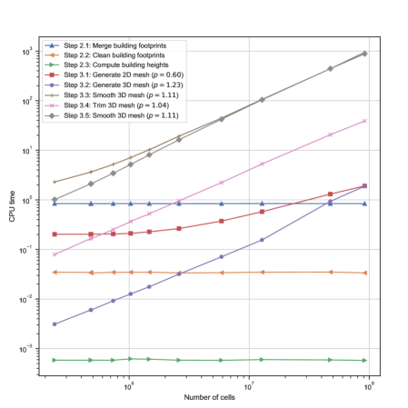
Figure 2: Benchmark study (a): Computational cost (CPU time) as function of the number of cells (tetrahedra) generated for the different steps of our mesh generation pipeline for the Majorna dataset.

Figure 3: Benchmark study (b): Computational cost (CPU time) as function of the number of buildings for the different steps of our mesh generation pipelline for the synthetic dataset.

3 Discussion

3.1 Findings

Our algorithm and implementation has proven to be generic and robust for a range of mesh resolutions, building densities, and also data quality. A substantial amount of work has gone into cleaning and filtering of data to ensure that the algorithm runs smoothly even for bad quality data. However, bad input data will lead to unexpected results. This can be seen in the top left corner of Figure 1 which shows a spike in the generated mesh. This spike is the result of a property being located at the site of one of the $107\text{\,}\mathrm{m}$ tall pylons of a bridge (Älvsborgsbron in Gothenburg, Sweden). This and other cases may be handled by more extensive filtering of the input data, such as ignoring detected “buildings” with aspect ratios larger than some limit.

Looking at the results of the benchmark study in Figure 2, we note that, as expected, the computational cost of Steps 2.1–2.3 is independent of the mesh resolution since those steps relate the cleaning and extraction of building heights from the raw data. For Steps 3.2–3.5, we see that the cost $T=T(N)$ as function of the number of cells is linear in $N$ ($p=1$ for $T\sim N^{p}$). For Step 3.1, the 2D mesh generation step, the cost scales like $N^{0.6}$, which agrees with linear scaling in the number of 2D cells generated ($N^{2/3}$). We conclude that the scaling of all steps of the mesh generation pipeline are optimal.

Turning now to Figure 3, the cost as function of the number of buildings, we see again good scaling for all steps; the cost of mesh generation is essentially constant as function of the number of buildings, as long as the city model contains a moderate number of buildings. When the number of buildings grow and the city model becomes very dense, the costs start to increase for all steps. For Steps 2.1–2.3, we expect a linear growth for all steps. This is also the case, except for Step 2.1 which exhibits an initial linear growth (when the number of buildings is small to moderate) and then a quadratic growth (for very dense city models). The quadratic growth at the extreme end is expected, even if binning is used (see Algorithm 1 below) since at the extreme, each building needs to be merged with all other buildings. This increase in cost is unproblematic since it only appears in extreme cases and the cost of merging is dominated by other costs (see Figure 2). For Steps 3.1–3.5, the costs start to grow when the number of buildings becomes large as a result of the city model becoming more complex and resulting in more cells being generated.

In summary, the results show optimal scaling in terms of both mesh resolution and the number of buildings. At the same time, there are large opportunities for optimisation through parallelism which we intend to investigate in future work.

3.2 Limitations

Substantial work has been put into or mesh generation pipeline. Nonetheless, there are known limitations that may be addressed in future work. We comment on some of these limitations here.

Only LoD1.2 supported

Our mesh generation pipeline currently only supports LoD1.2 city models (flat roofs). Work on extending the mesh generation pipeline to LoD1.3 and LoD2.x is in progress, based on a combination of machine learning for rooftop segmentation from orthophotos and 3D model generation from pointcloud data. Further extension to LoD3 would require street level imagery in order to get information about the building façades [34].

Lack of parallelism

Our implementation does not currently support any parallelism. One of the immediate planned steps is to extensively profile, optimize, and decide suitable parallelisation strategies for the different steps of the mesh generation pipeline. Parallelism will open up new possibilities, e.g., meshing of the whole of Sweden in tiles and stitching them together, in order to create a watertight mesh on a national level, similar to the 3D version of the Register of Buildings and Addresses of the Netherlands (https://3dbag.nl).

Lack of underground meshing

Our implementation only considers ground and buildings and does not take into account infrastructure like bridges or green areas. In addition, we currently only consider mesh generation of the volume above ground. In future work, we plan to also consider mesh generation of volumes below ground which is of importance for geotechnical simulation [35].

4 Methods

4.1 Overview of the mesh generation pipeline

The meshing pipeline consists of three main steps: (1) city model generation based on cadastral (2D) data and point cloud (3D) data; (2) simplification of the city model generated in the first step; and (3) mesh generation based on the simplified city model from the second step.

4.2 Step 1: Generate city model

In the first step of the mesh generation pipeline, 2D building footprints are extracted from the cadastral data and building heights are computed by sampling the point cloud for points that fall inside the building footprints. This results in a LoD1.2 city model represented as polygonal prisms $P\times[h_{0},h_{1}]$, where $P$ is the 2D polygon representing the building, $h_{0}$ is the ground height at the centre of the building, and $h_{1}$ is the absolute computed height of the building.

The processing pipeline involves several essential steps as outlined in Table 1. We comment briefly on some of these steps; full details are provided in the open-source implementation of the mesh generation pipeline [16].

Step 1.1	Read point cloud data (several LAS/LAZ files)
Step 1.2	Read building footprints (SHP file)
Step 1.3	Compute digital terrain map (DTM)
Step 1.4	Clean building footprints
Step 1.5	Extract building points (from point cloud data)
Step 1.6	Compute building heights (from building points and DTM)
Step 1.7	Export city model

Table 1: Essential substeps for Step 1: Generate city model.

Step 1.3: Compute digital terrain map (DTM)

The digital terrain map (DTM) is computed from the point cloud data by first constructing a regular 2D grid of the domain. The grid size is configurable and is set by default to $1\text{\,}\mathrm{m}$. We iterate over all the points in the point cloud and assign each point to a bin associated with its closest grid point. We then compute the mean of the heights ($z$-components) for each bin to set the mean of each grid point. This step is computationally inexpensive (of linear complexity) as it only involves iterating once over the point cloud. If the point cloud is of low quality (sparse), it may happen that the bins are empty for some grid points. To fill in the values for the missing grid points, the generation of the DTM is completed by a flood fill starting from the grid points on the boundary of empty regions. The generated DTM may be sampled at arbitrary points within the computational domain and returns the value at the given point by bilinear interpolation using the four closest grid points (which may be computed without searching).

Step 1.4: Clean building footprints

Each building footprint (polygon) is processed to ensure that the polygons are closed, oriented (counter clock-wise) and that there are no duplicate vertices or consecutive parallel edges. This step is necessary since the raw data typically contains a mix of closed and non-closed polygons with multiple duplicate vertices and edges.

Step 1.5: Extract building points (from point cloud data)

For each building, we extract all points of the point cloud that fall within a margin of the the building footprint. This step is potentially costly since a naïve implementation would involve searching through the entire point cloud for each building. To avoid a costly search, we build for both the set of building footprints and the point cloud an axis-algined bounding box (AABB) tree and then compute the collision between the two AABB trees following standard algorithms from computational geometry [36]. The result of the collision between the two trees is a list of collision candidates; that is, a list of pairs consisting of a point and a bounding box. Each such pair signifies a point from the point cloud found to be located within the bounding box of a building footprint.

Once the collision candidates have been computed, the candidates are filtered to check whether the points actually fall within the corresponding building footprint (not just within its bounding box). This filtering relies on a point-in-polygon algorithm, which is efficiently implemented based on computing the quadrant angle [37] for each such point in relation to the polygon.

The filtered points are classified as either “roof points” or “ground points”. Roof points are those that fall within the building footprint and have LiDAR point classification 6 (Building). Ground points are those that fall outside the building footprint but closer than a configurable margin (by default $1\text{\,}\mathrm{m}$) to the building footprint and have LiDAR point classification 2 or 9 (Ground or Water). Both roof points and ground points are filtered for outliers, removing all points that fall outside two standard deviations.

Step 1.6: Compute building heights (from building points and DTM)

Building heights are computed by examining for each building its ground points and building points from the previous step. The ground height $h_{0}$ of the building is set to the 10th percentile of the ground points and the roof height $h_{1}$ is set to the 90th percentile of the roof points. If ground points are missing, then the ground height $h_{0}$ is computed by sampling the DTM at the center of the building footprint. Finally, the generated city model is exported to a simple JSON format.

4.3 Step 2: Simplify city model

The result of Step 1 is a clean LoD1.2 city model consisting of a set of buildings, each defined by a 2D polygonal footprint, a ground height and a roof height, together with a digital terrain map that may be sampled to give the ground height at any point within the computational domain. However, before a mesh can be generated from the city model, the city model must be simplified. Simplification is necessary since building footprints may be located at arbitrarily small distances or even overlap, which may cause the mesh generation to either break down or become prohibitively costly by needing to resolve tiny gaps between buildings. The key steps in the simplification are outlined in Table 2.

Step 2.1	Merge building footprints
Step 2.2	Clean building footprints
Step 2.3	Compute building heights
Step 2.4	Export city model

Table 2: Essential substeps for Step 2: Simplify city model.

Step 2.1: Merge building footprints

To prevent very small or even zero distances between buildings, all pairs of buildings that are closer than a configurable threshold distance (by default $1\text{\,}\mathrm{m}$) are merged into a single building.

The merging process is outlined in Algorithm 1. The algorithm starts from the city model generated in Step 1 and adds all buildings to a queue. It then proceeds to pop the first building from the queue and iterates over all other buildings. If the distance between any such pair of buildings is found to be closer than the threshold distance $\varepsilon>0$, the two building footprints are merged using Algorithm 2 (described below) and the new building is pushed to (added to the back of) the queue. The algorithm proceeds until the queue is empty.

Algorithm 1 MergeCityModel (for details, refer to [16])

1:Array $[P_{i}]_{i=1}^{n}$ of building footprint polygons

2:Threshold distance $\varepsilon>0$

3:Initialize regular grid with resolution $h>\varepsilon$

4:for $i\in[1,n]$ do

5:    $\mathcal{B}_{i}\leftarrow$ bins (grid points) closer than $h$ to $P_{i}$

6:end for

7:Initialize empty $queue$

8:for $i\in[1,n]$ do

9:    Push $i$ to $queue$

10:end for

11:while $queue$ not empty do

12:    Pop $i$ from $queue$

13:    $\mathcal{J}\leftarrow\{j\in[1,n]\;|\;\mathcal{B}_{i}\cap\mathcal{B}_{j}\neq\emptyset\}$

14:    for $j\in\mathcal{J}$ do

15:         if $i\neq j$ and $P_{j}$ not empty then

16:             if $\|P_{i}-P_{j}\|<\varepsilon$ then

17:                 $P_{i}\leftarrow$ MergePolygons($P_{i}$, $P_{j}$)

18:                 Push $i$ to $queue$

19:                 $\mathcal{B}_{i}\leftarrow$ bins (grid points) closer than $h$ to $P_{i}$

20:                 $P_{j}\leftarrow\emptyset$

21:             end if

22:         end if

23:    end for

24:end while

A simple binning strategy is used to avoid the otherwise quadratic cost associated with searching all buildings for overlap/closeness. The binning is based on covering the computational domain by a regular grid and associating each building (polygon footprint) to all bins (grid points) such that the (bounding box of) the polygon is closer than the grid size $h$. This ensures that two buildings closer than the threshold $\varepsilon>0$ must always be associated with a common bin (grid point), as long as $h>\varepsilon$. Particular care is required in the binning implementation to ensure that the binning works correctly in the face of numerical rounding errors. As long as $h>\varepsilon$, the grid size is arbitrary and numerical experiments indicate that a factor $1$ to $4$ times the mean building footprint diameter is a good choice. Our current implementation uses the factor $4$.

Algorithm 2 takes two building footprints (polygons) and returns a single, simple polygon by heuristically merging the two polygons. Note that only in the case of two intersecting polygonal domains is it clear what shape the merging algorithm should create, namely the (polygonal boundary of the) union of the two polygonal domains. In all other cases, if the polygons do not intersect, a heuristic choice must be made as to how a new shape should be created from the two building footprints. Algorithm 2 first attempts to compute the union of the two polygons. If the resulting shape is acceptable, the union is returned; a shape is acceptable if it is a simple polygon and the following two conditions are met: (i) no two distinct vertices are separated by less than the threshold $\varepsilon$ and (ii) no vertex is closer than $\varepsilon$ to an edge of which it is not an endpoint. If the union is not acceptible, the algorithm projects the vertices of each of the two polygons onto the edges of the other polygon (only for vertices that are deemed close to the other polygon); see Algorithm 3. The convex hull of those projected vertices defines a patch $P$ and the union $A\cup B\cup P$ is then tested for acceptance in the same way. If the patch is not accepted, then the patch is grown iteratively (by including more vertices). If this process fails, the algorithm checks the union of the convex hulls of both polygons, and in the worst-case scenaro, the convex hull of the two polygons is used.

Algorithms 1–3 are implemented as part of DTCC Builder [16]. For geometric predicates and set operations, the GEOS is a C/C++ library is used. [38]

Algorithm 2 MergePolygons (for details, refer to [16])

1:Polygon $A$ and polygon $B$

2:Threshold distance $\varepsilon>0$ $\triangleright$ Default value used is $\varepsilon=1\mathrm{m}$

3:Maximum iterations $N>0$ $\triangleright$ Default value used is $N=3$

4:$C\leftarrow A\cup B$ $\triangleright$ Compute union $C$ of $A$ and $B$

5:if IsValid($C$, $\varepsilon$) then $\triangleright$ Check if $C$ should be accepted

6:    return $C$

7:end if

8:for $k\in[1,N]$ do $\triangleright$ Iterate with increasing threshold

9:    $P_{A}\leftarrow\text{VertexProjections($A$, $B$, $\varepsilon$)}$ $\triangleright$ Compute projection of vertices of $A$ onto $B$

10:    $P_{B}\leftarrow\text{VertexProjections($B$, $A$, $\varepsilon$)}$ $\triangleright$ Compute projection of vertices of $B$ onto $A$

11:    $P\leftarrow$ ConvexHull($P_{A}\cup P_{B}$) $\triangleright$ Compute convex hull $P$ of vertex projections

12:    $C\leftarrow A\cup B\cup P$ $\triangleright$ Compute union $C$ of $A$, $B$ and $P$

13:    if IsValid($C$, $\varepsilon$) then $\triangleright$ Check if $C$ should be accepted

14:         return $C$

15:    end if

16:    $\varepsilon\leftarrow 2\varepsilon$ $\triangleright$ Increase tolerance

17:end for

18:$C\leftarrow\text{ConvexHull($A$)}\cup\text{ConvexHull($B$)}$ $\triangleright$ Compute union $C$ of convex hulls

19:if IsValid($C$, $\varepsilon$) then $\triangleright$ Check if $C$ should be accepted

20:    return $C$

21:end if

22:$C\leftarrow\text{ConvexHull($A\cup B$)}$ $\triangleright$ Fall back to convex hull of union

23:return $C$

Algorithm 3 VertexProjections (for details, refer to [16])

1:Polygon $A$ and polygon $B$

2:Threshold distance $\varepsilon>0$ $\triangleright$ Default value used is $\varepsilon=1\mathrm{m}$

3:$P\leftarrow\emptyset$ $\triangleright$ Initialize empty set of points

4:for $v\in\mathrm{Vertices}(A)$ do $\triangleright$ Iterate over vertices of $A$

5:    for $e\in\mathrm{Edges}(B)$ do $\triangleright$ Iterate over edges of $B$

6:         $p\leftarrow\operatorname*{arg\,min}_{q\in e}\|v-q\|$ $\triangleright$ Compute closest point on edge

7:         if $\|v-p\|<\varepsilon$ then $\triangleright$ Check if point is close enough

8:             $P\leftarrow P\cup\{p\}$ $\triangleright$ Add point

9:         end if

10:    end for

11:end for

A number of examples of merged polygons generated by Algorithm 2 are provided in Figure 4 (simple test cases) and Figure 5 (real-world data). The algorithm handles the majority of building polygons very well but occasionally fails in a few corner cases. It then falls back to computing the convex hull of the two buildings, which is often a satisfactory resolution.

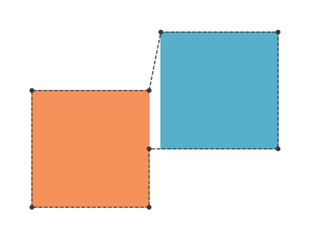
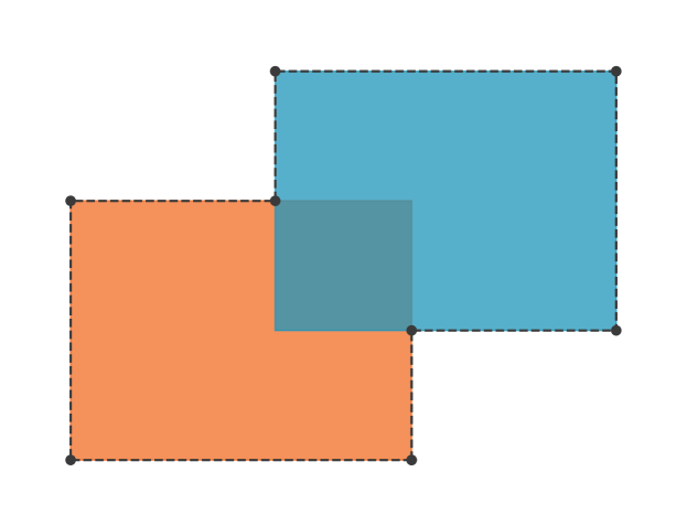
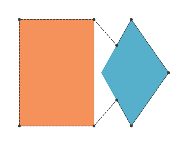
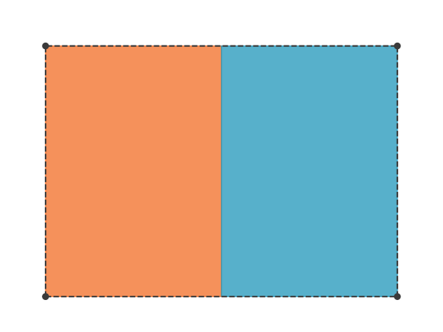
Figure 4: Examples of merged building footprints generated by Algorithm 2 for a selection of simple test cases. In each panel, the two colored shapes show the two polygons to be merged and the dashed line and marked vertices show the result of the merging algorithm.

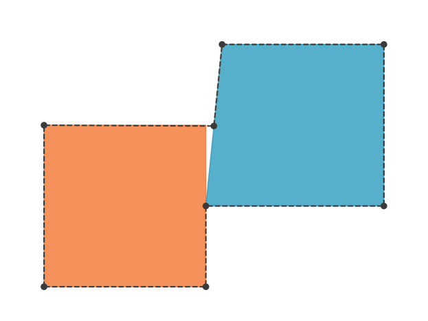
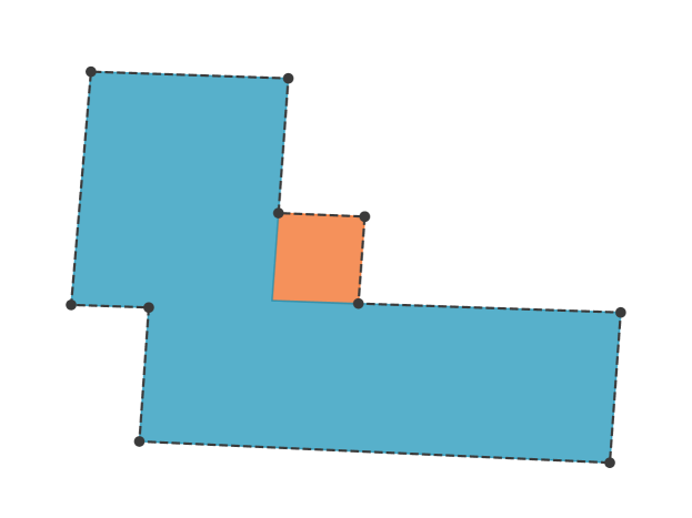
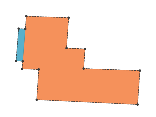
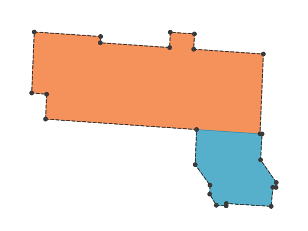
Figure 5: Examples of merged building footprints generated by Algorithm 2 for the Hammarkullen test case. In each panel, the two colored shapes show the two polygons to be merged and the dashed line and marked vertices show the result of the merging algorithm.

Steps 2.2–2.4

Step 2.1 potentially reduces the number buildings in the city model when two or more buildings are merged into a single building. After having completed Step 2.1, the city model is once again cleaned in Step 2.2 (same as Step 1.4) and then all building heights are recomputed; when two buildings are merged, their ground points and roof points (computed in Step 1.6) are also merged and used for (re)computing the heights in Step 2.3. Finally, the city model is (re)exported to JSON format in Step 2.4.

4.4 Step 3: Generate city mesh

After the completion of Step 2, the city model has been generated, cleaned and simplified and is now suitable as input for the mesh generation step. The key idea of the mesh generation is to first generate a 2D mesh that respects the footprints of the building footprints and then layer and transform the 2D mesh to create a 3D volume mesh of the city model. The key steps in the mesh generation process are outlined in Table 3.

Step 3.1	Generate 2D mesh
Step 3.2	Generate 3D mesh (layer 2D mesh)
Step 3.3	Smooth 3D mesh (set ground height)
Step 3.4	Trim 3D mesh (remove building interiors)
Step 3.5	Smooth 3D mesh (set ground and building heights)
Step 3.6	Export mesh

Table 3: Essential substeps for Step 3: Generate city mesh.

Step 3.1: Generate 2D mesh

A 2D mesh is generated of the computational domain (a bounding box enclosing the city model) that respects the footprint of each building of the (simplified) city model from Step 2. The mesh is generated by including the edges of all building footprints as segments that must be included in the triangular mesh generated by the 2D mesh generator. The 2D mesh generator used is Triangle [39], which is a well-proven, robust and efficient 2D mesh generator that generates triangular meshes of high quality. Figure 6 illustrates the output of Step 3.1.

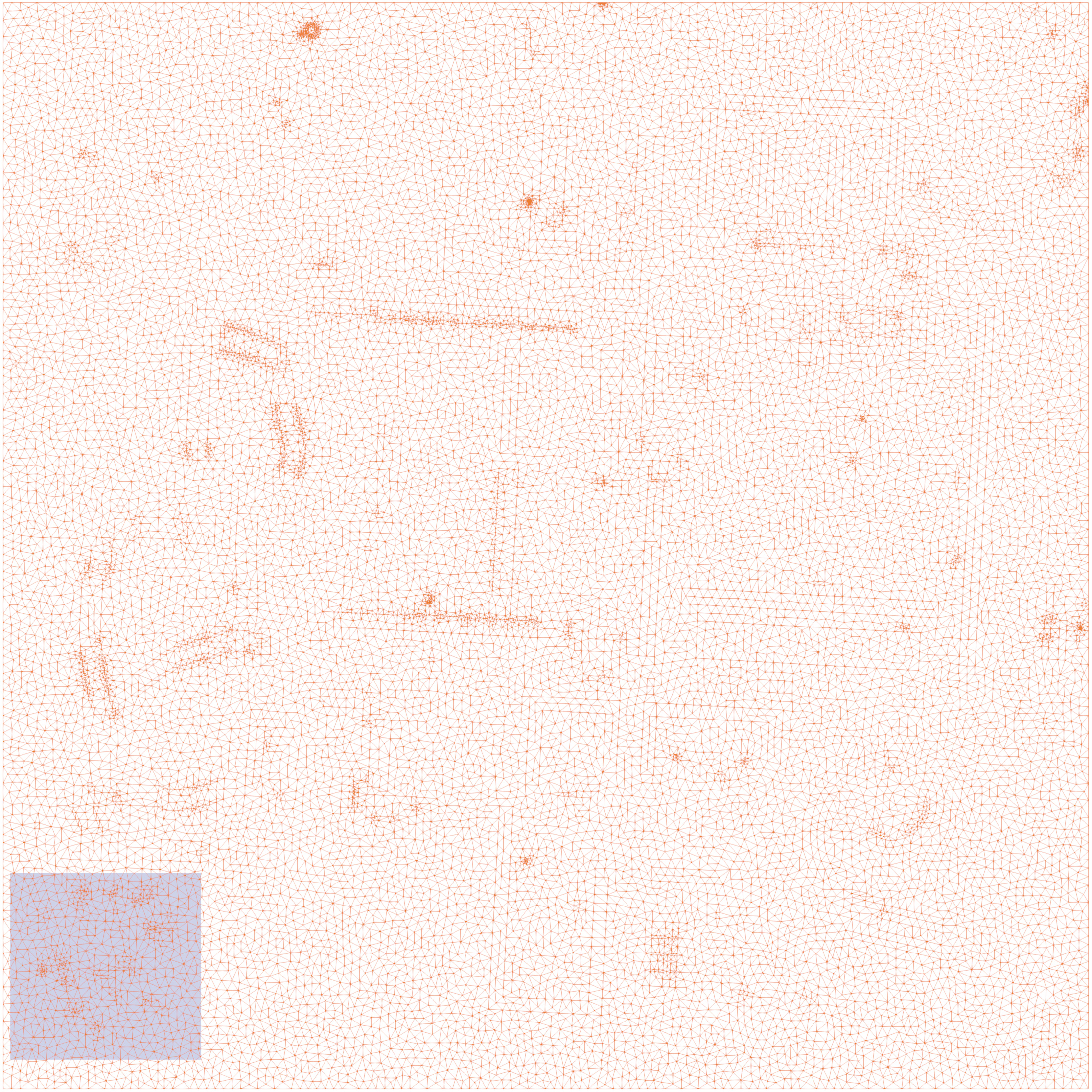
(a) Full view

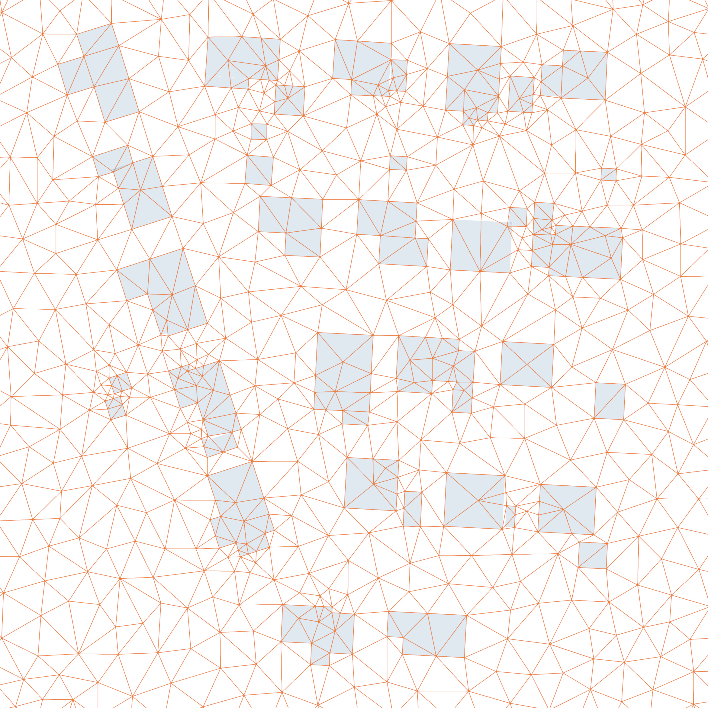
(b) Detail

Figure 6: Output from Step 3.1 in the 3D mesh generation process for the Hammarkullen test case.

Step 3.2: Generate 3D mesh (layer 2D mesh)

Once the 2D mesh is generated, a 3D mesh is created by layering the 2D mesh. The distance between the layers is set to the same mesh size used for the 2D mesh generation in Step 3.1 and the number of layers is determined by a given height of the computational domain.

The layering creates a 3D mesh of triangular prisms. Each such prism is then divided into three tetrahedra. By following a consistent numbering scheme of the triangles in the triangular mesh, we may ensure that the generated 3D tetrahedral mesh is conforming; that is, the intersection between each pair of tetrahedra is either the empty set, a common vertex, a common edge, or a common face (no hanging nodes).

To be precise, let $u_{1}$, $u_{2}$, $u_{3}$ be the indices of the three vertices that define a triangle in any given layer, and let $v_{1}$, $v_{2}$, $v_{3}$ be the indices for the corresponding triangle in the next layer. It is assumed that the vertices of each triangle are sorted by global vertex index such that $u_{1}<u_{2}<u_{3}$ and $v_{1}<v_{2}<v_{3}$. We then divide the prism defined by the two triangles into three tetrahedra by

$$T_{1} =(u_{1},u_{2},u_{3},v_{3})$$ (1)

$$T_{2} =(u_{1},v_{2},u_{2},v_{3})$$ (2)

$$T_{3} =(u_{1},v_{1},v_{2},v_{3})$$ (3)

This numbering, in combination with the requirement that each triangle be sorted by global vertex index, ensures that the tetrahedra created from any two neighboring triangular prisms are matching on their common boundary. See Figure 7 for an illustration.

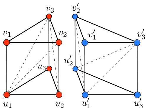
Figure 7: The triangular prisms created by layering the 2D mesh are divided into three tetrahedra in such a way that the tetrahedra generated from two neighboring prisms are always matching on the common boundary.

The result of Step 3.2 is a tetrahedral (volume) 3D mesh of the bounding box of the computational domain, where the tetrahedral faces are ensured to respect the building boundaries. Figure 8(a) illustrates the output of Step 3.2.

Step 3.3: Smooth 3D mesh (set ground height)

The 3D mesh generated in Step 3.2 is next transformed to take the topography of the city into account; that is, the mesh is transformed to set the ground height as defined by the digital terrain map (DTM) generated in Step 1.3. Note that we cannot simply displace the mesh vertices at ground level to account for the ground height, since this would (potentially and very likely) generate inverted tetrahedra by pushing the vertices in the first layer past the vertices in the second layer and beyond. Instead, we employ Laplacian mesh smoothing [40] with the ground height as a boundary condition. This results in a smooth transformation of the mesh that displaces the vertices in all layers, with the vertices in the first layer set to the height given by the DTM.

Laplacian smoothing is based on solving a partial differential equation (PDE), the solution of which defines the displacement of each vertex of the mesh. To define the PDE, let $\Omega$ be the computational domain defined by the 3D mesh, let $\Gamma_{\mathrm{G}}$ be the ground layer of the domain, and let $\mathrm{DTM}:\mathbb{R}^{2}\to\mathbb{R}$ be the function defining the digital terrain map, defining the ground height at any given point.

We solve the following boundary value problem for the $z$-displacement of the 3D mesh:

$$-\Delta u =0 \text{in }\Omega$$ (4)

$$u(x,y,z) =\mathrm{DTM}(x,y)-z \text{on }\Gamma_{\mathrm{G}}$$ (5)

$$\partial_{n}u(x,y,z) =0 \text{on }\partial\Omega\setminus\Gamma_{\mathrm{G}}$$ (6)

Note that we thus solve a boundary value problem with the differential ground height as a strong (Dirichlet) boundary condition at the bottom of the computational domain, and homogeneous Neumann conditions on the remaining boundary. The boundary value problem is defined and solved using FEniCS [41] with linear ($P_{1}$) elements. The linear system is solved using the BiCGSTAB Krylov method [42] and an algebraic multigrid (AMG) preconditioner.

Once the solution has been computed, the $z$-displacement $u$ is added to each vertex of the 3D mesh to obtain a transformed mesh that respects the ground height. Figure 8(b) illustrates the output of Step 3.3.

Step 3.4: Trim 3D mesh (remove building interiors)

The mesh obtained from Step 3.3 respects the ground height and the faces of all tetrahedra respect the building boundaries. However, the mesh still covers the entire computational domain, including the interior of buildings. In Step 3.4, we trim the 3D mesh to remove all tetrahedra from building interiors. Figure 8(c) illustrates the output of Step 3.4.

Step 3.5: Smooth 3D mesh (set ground and building heights)

The mesh obtained from Step 3.4 is almost complete. However, the trimming process can only decide to either keep or remove tetrahedra. As a result, the height of each building will be set to the height of the closest layer, and the height of each building will be correct only to within the mesh size used define the layer distance. To obtain correct building heights, we once again perform Laplacian smoothing as in Step 3.3, this time by solving the following boundary value problem:

$$-\Delta u =0 \text{in }\Omega$$ (7)

$$u(x,y,z) =\mathrm{DTM}(x,y)-z \text{on }\Gamma_{\mathrm{G}}$$ (8)

$$u(x,y,z) =\mathrm{BH}(x,y)-z \text{on }\Gamma_{\mathrm{R}}$$ (9)

$$\partial_{n}u(x,y,z) =0 \text{on }\partial\Omega\setminus(\Gamma_{\mathrm{G}}\cup\Gamma_{\mathrm{R}})$$ (10)

where $\Gamma_{\mathrm{R}}$ is the part of the boundary touching building roof tops and where $\mathrm{BH}:\mathbb{R}^{2}\to\mathbb{R}$ is a function defining the (absolute) building heights (computed in Step 2.3).

Note that in total two smoothing steps are performed, both before (Step 3.2) and after (Step 3.4) trimming the mesh from tetrahedra inside buildings. Two steps are essential to avoid the generation of inverted tetrahedra; if the first smothing step is skipped and only the second smoothing step is performed, then the second smoothing step will be too agressive and will result in inverted tetrahedra in regions close to building roof tops.

The result of Step 3.5 is the final tetrahedral 3D volume mesh of the city model. The mesh is stored as a list of vertex positions and a list of tetrahedral vertex indices as in [43]. The mesh discretizes the volume defined by subtracting from a bounding box of the city model both the ground and the buildings. Figure 8(d) illustrates the output of Step 3.5.

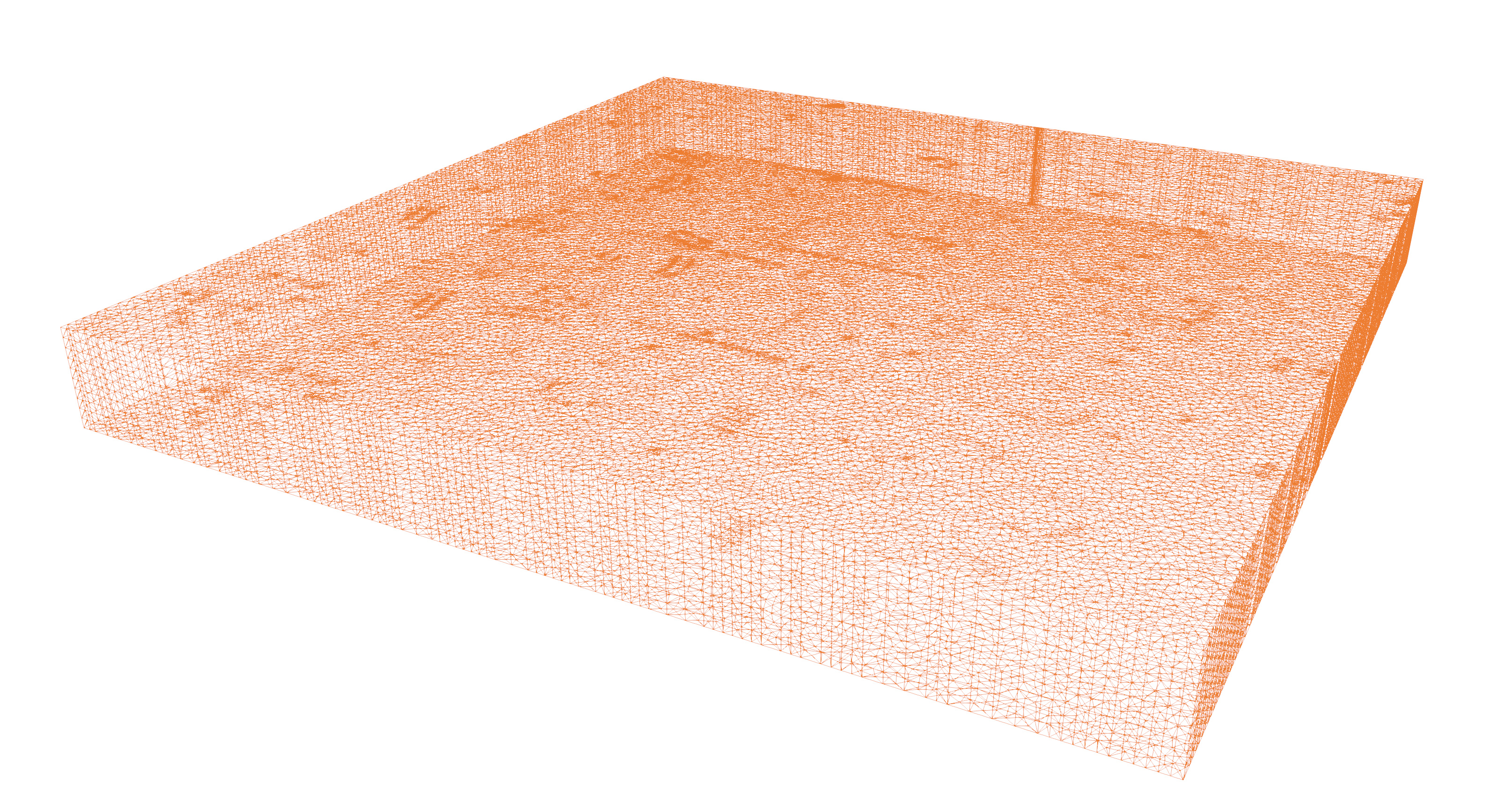
(a) Step 3.2

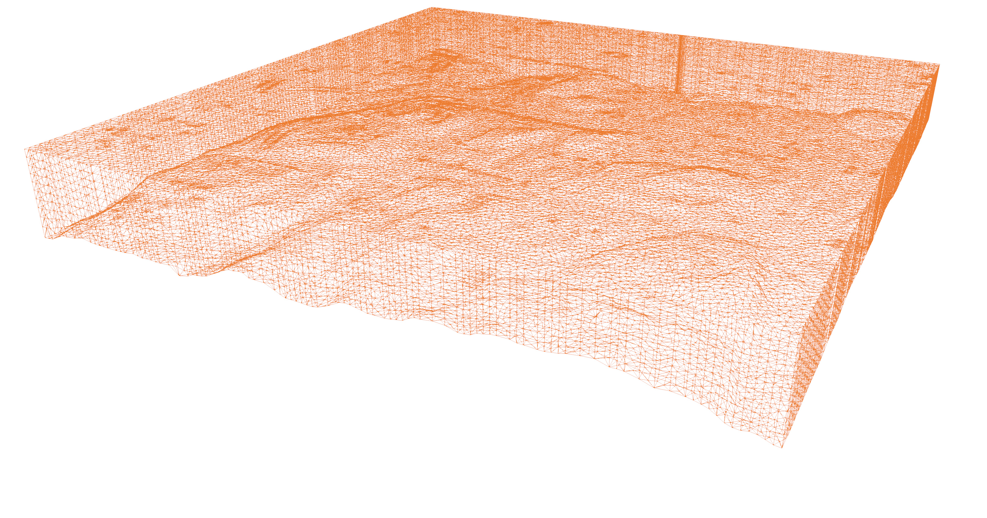
(b) Step 3.3

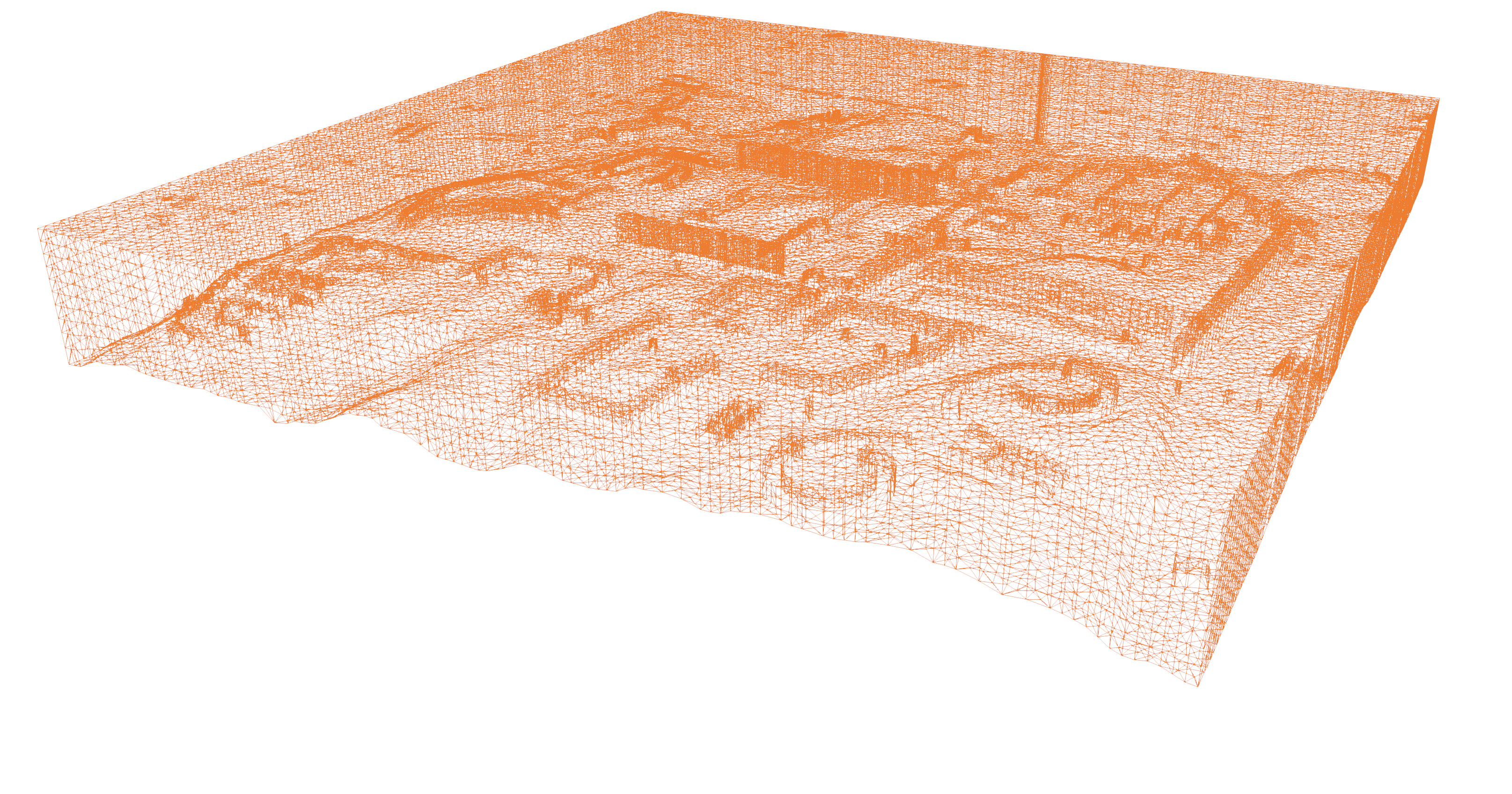
(c) Step 3.4

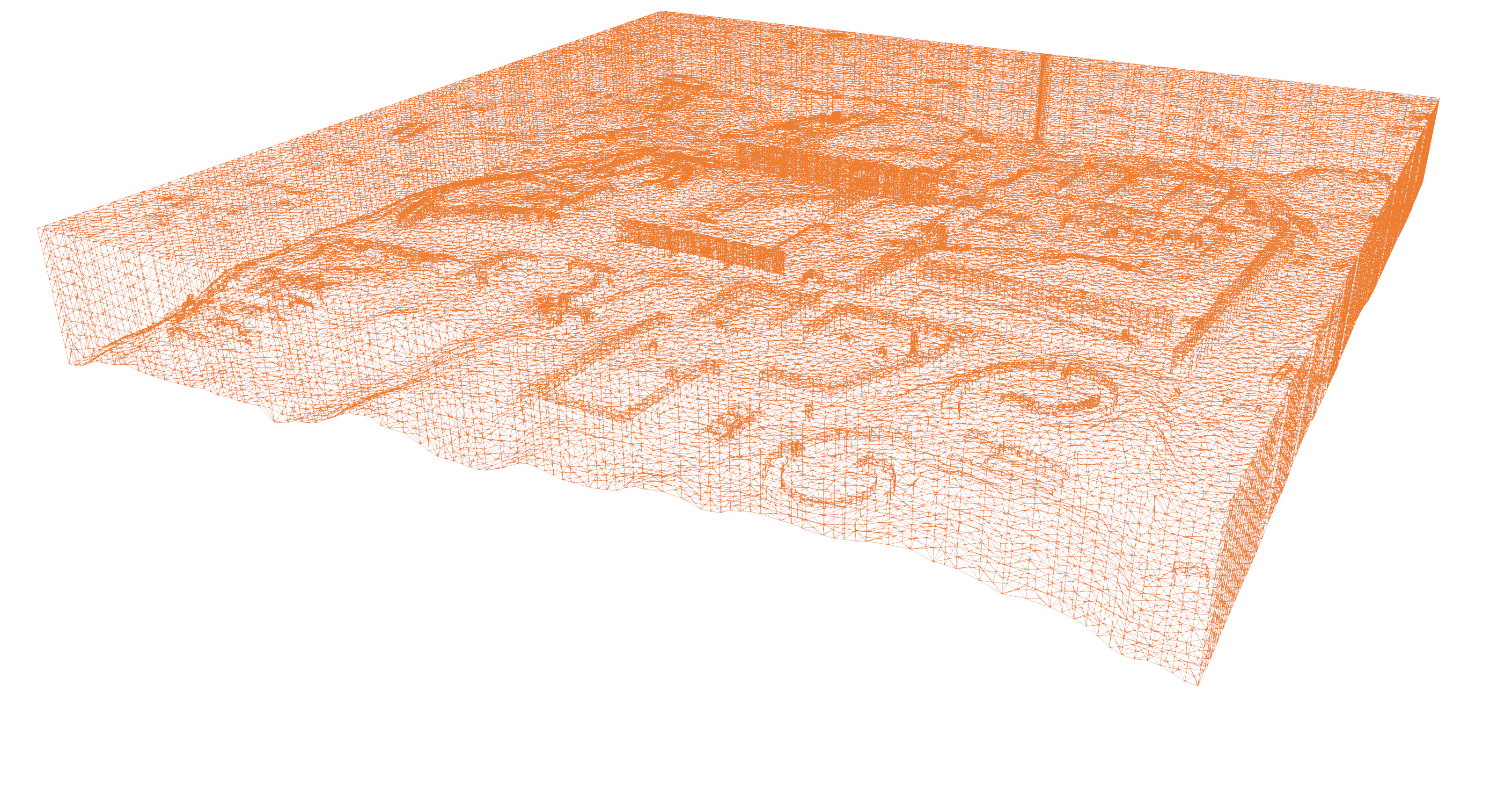
(d) Step 3.5

Figure 8: Output from Steps 3.2–3.5 in the 3D mesh generation process for the Hammarkullen test case.

4.5 Data sources

All data used in this study are public data obtained from the Swedish Mapping, Cadastral and Land Registration Authority. In particular, we have used the dataset "Lantmäteriet:
Laserdata NH 2019" in LAZ format for point clouds and the dataset "Lantmäteriet:
Fastighetskartan bebyggelse 2020" in SHP format for cadastral data (building footprints). The data are in reference to the standard coordinate system for Sweden, EPSG:3006 also known as SWEREF99 TM. The resolution of the point clouds used is specified to between 0.5 and 1 points per square meter. Two different datasets were used in this study, Majorna and Hammarkullen, two regions in Gotheburg, Sweden. The dataset Majorna, used for the benchmark study, is freely distributable from Lantmäteriet and can be accessed through the Git repository of our implementation [16]. The dataset Hammarkullen, used for illustrations in the Methods section, is public data but requires a license from Lantmäteriet and may thus not be shared as part of our implementation.

4.6 Implementation

The algorithms described in this paper are implemented as part of the open-source (MIT license) digital twin platform developed at the the Digital Twin Cities Centre
(https://dtcc.chalmers.se). In particular, the software and data used to generate the results presented in this paper are availalable as part of DTCC Builder version [16]. The algorithms are implemented in C++ and use several open-source packages, notably FEniCS [41] for solving PDEs, Triangle [39] for 2D mesh generation, and GEOS [38] for geometric operations.

5 Acknowledgments

Both authors gratefully acknowledge valuable input from Dag Wästberg on geodata processing, Jorge Gil and Nikos Pitsianis for insightful discussions, and Orfeas Eleftheriou and Sanjay Somanath for valuable assistance with this study. This work is part of the Digital Twin Cities Centre supported by Sweden’s Innovation Agency Vinnova under Grant No. 2019-00041.

References

- [1] Bernd Ketzler, Vasilis Naserentin, Fabio Latino, Christopher Zangelidis, Liane Thuvander, and Anders Logg. Digital Twins for Cities: A State of the Art Review. Built Environment, 46(4):547–573, 2020.
- [2] Mengnan Liu, Shuiliang Fang, Huiyue Dong, and Cunzhi Xu. Review of digital twin about concepts, technologies, and industrial applications. Journal of Manufacturing Systems, 58:346–361, January 2021.
- [3] Hamid Reza Ranjbar, Ali Reza Gharagozlou, and Ali Reza Vafaei Nejad. 3D Analysis and Investigation of Traffic Noise Impact from Hemmat Highway Located in Tehran on Buildings and Surrounding Areas. Journal of Geographic Information System, 04(04):322–334, 2012.
- [4] Esther Rivas, Jose Luis Santiago, Yolanda Lechón, Fernando Martín, Arturo Ariño, Juan José Pons, and Jesús Miguel Santamaría. CFD modelling of air quality in Pamplona City (Spain): Assessment, stations spatial representativeness and health impacts valuation. Science of The Total Environment, 649:1362–1380, February 2019.
- [5] Jean-Marie Bahu, Andreas Koch, Enrique Kremers, and Syed Monjur Murshed. Towards a 3D spatial urban energy modelling approach. International Journal of 3-D Information Modeling (IJ3DIM), 3(3):1–16, 2014.
- [6] Alina Galimshina, Maliki Moustapha, Alexander Hollberg, Pierryves Padey, Sébastien Lasvaux, Bruno Sudret, and Guillaume Habert. What is the optimal robust environmental and cost-effective solution for building renovation? Not the usual one. Energy and Buildings, 251:111329, 2021.
- [7] Aneta Strzalka, Jürgen Bogdahn, Volker Coors, and Ursula Eicker. 3D City modeling for urban scale heating energy demand forecasting. HVAC and R Research, 17(4):526–539, 2011.
- [8] Felix Heisel, Joseph McGranahan, Joseph Ferdinando, and Timur Dogan. High-resolution combined building stock and building energy modeling to evaluate whole-life carbon emissions and saving potentials at the building and urban scale. Resources, Conservation and Recycling, 177:106000, 2022.
- [9] C. Pettit, I. Widjaja, P. Russoa, R. Sinnott, R. Stimson, and M. Tomko. VISUALISATION SUPPORT FOR EXPLORING URBAN SPACE AND PLACE. Technical report.
- [10] Zhihang Yao, Claus Nagel, Felix Kunde, György Hudra, Philipp Willkomm, Andreas Donaubauer, Thomas Adolphi, and Thomas H. Kolbe. 3DCityDB - a 3D geodatabase solution for the management, analysis, and visualization of semantic 3D city models based on CityGML. Open Geospatial Data, Software and Standards, 2018.
- [11] Hugo Ledoux, Ken Arroyo Ohori, Kavisha Kumar, Balázs Dukai, Anna Labetski, and Stelios Vitalis. CityJSON: A compact and easy-to-use encoding of the CityGML data model. Open Geospatial Data, Software and Standards, 2019.
- [12] Ken Arroyo Ohori, Filip Biljecki, Kavisha Kumar, Hugo Ledoux, and Jantien Stoter. Modeling cities and landscapes in 3D with CityGML. In Building Information Modeling, pages 199–215. Springer, 2018.
- [13] F. Biljecki, H. Ledoux, X. Du, J. Stoter, K. H. Soon, and V. H. S. Khoo. THE MOST COMMON GEOMETRIC and SEMANTIC ERRORS in CITYGML DATASETS. In ISPRS Annals of the Photogrammetry, Remote Sensing and Spatial Information Sciences, volume 4, pages 13–22. Copernicus GmbH, October 2016.
- [14] Hugo Ledoux, Filip Biljecki, Balázs Dukai, Kavisha Kumar, Ravi Peters, Jantien Stoter, and Tom Commandeur. 3dfier: Automatic reconstruction of 3D city models. Journal of Open Source Software, 6(57):2866, January 2021.
- [15] Filip Biljecki, Hugo Ledoux, Jantien Stoter, and Junqiao Zhao. Formalisation of the level of detail in 3D city modelling. Computers, Environment and Urban Systems, 48:1–15, 2014.
- [16] Anders Logg, Vasilis Naserentin, and Dag Wästberg. DTCC Builder. Digital Twin Cities Centre, 2022.
- [17] Ruisheng Wang, Jiju Peethambaran, and Dong Chen. LiDAR Point Clouds to 3-D Urban Models : A Review. IEEE Journal of Selected Topics in Applied Earth Observations and Remote Sensing, 11(2):606–627, February 2018.
- [18] Mehmet Buyukdemircioglu and Sultan Kocaman. A 3D campus application based on city models and WebGL. In International Archives of the Photogrammetry, Remote Sensing and Spatial Information Sciences - ISPRS Archives, volume 42, pages 161–165. International Society for Photogrammetry and Remote Sensing, November 2018.
- [19] Felix Tschirschwitz, Christian Richerzhagen, Heinz Jürgen Przybilla, and Thomas P. Kersten. Duisburg 1566: Transferring a Historic 3D City Model from Google Earth into a Virtual Reality Application. PFG - Journal of Photogrammetry, Remote Sensing and Geoinformation Science, 87(1-2):47–56, June 2019.
- [20] Iñaki Prieto, Jose Luis Izkara, and Elena Usobiaga. The application of LiDAR data for the solar potential analysis based on urban 3D model. Remote Sensing, 11(20), October 2019.
- [21] Fredrik Lindberg, Per Jonsson, Tsuyoshi Honjo, and Dag Wästberg. Solar energy on building envelopes - 3D modelling in a 2D environment. Solar Energy, 115:369–378, May 2015.
- [22] H. Jian and X. Fan. Three-dimensional visualization of harmful gas diffusion in an urban area. In IOP Conference Series: Earth and Environmental Science, volume 18. Institute of Physics Publishing, 2014.
- [23] Guo Huadong. DIGITAL EARTH SCIENCE PLATFORM: DESP/CAS. Technical report.
- [24] N. R. Rajpriya, Anjana Vyas, and S. A. Sharma. Generation of 3D model for Urban area using Ikonos and Cartosat-1 satellite imageries with RS and GIS techniques. In International Archives of the Photogrammetry, Remote Sensing and Spatial Information Sciences - ISPRS Archives, volume 40, pages 899–906. International Society for Photogrammetry and Remote Sensing, 2014.
- [25] P. Nageler, G. Zahrer, R. Heimrath, T. Mach, F. Mauthner, I. Leusbrock, H. Schranzhofer, and C. Hochenauer. Novel validated method for GIS based automated dynamic urban building energy simulations. Energy, 139:142–154, 2017.
- [26] Yiqun Chen, Erfan Shooraj, Abbas Rajabifard, and Soheil Sabri. From IFC to 3D Tiles: An Integrated Open-Source Solution for Visualising BIMs on Cesium.
- [27] Tomo Cerovsek. A review and outlook for a ‘Building Information Model’ (BIM): A multi-standpoint framework for technological development. Advanced Engineering Informatics, 25(2):224–244, April 2011.
- [28] Gustavo Alomia, Xun Luo, Claudia Zuniga, Andres Navarro Cadavid, and Carlos Lozano-Garzon. Automatic 3D urban installation generation in virtual cities. In Proceedings - 2019 International Conference on Virtual Reality and Visualization, ICVRV 2019, pages 217–222. Institute of Electrical and Electronics Engineers Inc., November 2019.
- [29] Nikolas Prechtel. On strategies and automation in upgrading 2D to 3D landscape representations. Cartography and Geographic Information Science, 42(3):244–258, May 2015.
- [30] Rico Richter and Jürgen Döllner. Concepts and techniques for integration, analysis and visualization of massive 3D point clouds. Computers, Environment and Urban Systems, 45:114–124, 2014.
- [31] Pavel Tobiáš, Jiří Cajthaml, and Jiří Krejčí. Rapid reconstruction of historical urban landscape: The surroundings of Czech chateaux and castles. Journal of Cultural Heritage, 30:1–9, March 2018.
- [32] Ivan Pađen, Clara García-Sánchez, and Hugo Ledoux. Towards automatic reconstruction of 3D city models tailored for urban flow simulations. Frontiers in Built Environment, 8, 2022.
- [33] H. G. Weller, G. Tabor, H. Jasak, and C. Fureby. A tensorial approach to computational continuum mechanics using object-oriented techniques. Computers in Physics, 12(6):620–631, November 1998.
- [34] Nikolai Kolibarov, Vasilis Naserentin, Dag Wastberg, Dessislava Petrova-Antonova, Sylvia Illieva, and Anders Logg. Towards LOD2+ Digital Twin for Cities Generation. In IFAC Workshop on Control for Smart Cities, 2022.
- [35] Johannes Tornborg, Mats Karlsson, Anders Kullingsjö, and Minna Karstunen. Modelling the construction and long-term response of Göta Tunnel. Computers and Geotechnics, 134:104027, 2021.
- [36] Christer Ericson. Real-Time Collision Detection. Crc Press, 2004.
- [37] Kai Hormann and Alexander Agathos. The point in polygon problem for arbitrary polygons. Computational geometry, 20(3):131–144, 2001.
- [38] GEOS contributors. GEOS Coordinate Transformation Software Library. Open Source Geospatial Foundation, 2021.
- [39] Jonathan Richard Shewchuk. Triangle: Engineering a 2D quality mesh generator and Delaunay triangulator. In Workshop on Applied Computational Geometry, pages 203–222. Springer, 1996.
- [40] David A Field. Laplacian smoothing and Delaunay triangulations. Communications in applied numerical methods, 4(6):709–712, 1988.
- [41] Anders Logg, Kent-Andre Mardal, and Garth Wells. Automated Solution of Differential Equations by the Finite Element Method: The FEniCS Book, volume 84. Springer Science & Business Media, 2012.
- [42] Henk A Van der Vorst. Bi-CGSTAB: A fast and smoothly converging variant of Bi-CG for the solution of nonsymmetric linear systems. SIAM Journal on scientific and Statistical Computing, 13(2):631–644, 1992.
- [43] Anders Logg. Efficient representation of computational meshes. International Journal of Computational Science and Engineering, 4(4), 2009.