Estimation of Doubly-Dispersive Channels in Linearly Precoded Multicarrier Systems Using Smoothness Regularization

Abstract

In this paper, we propose a novel channel estimation scheme for pulse-shaped multicarrier systems using smoothness regularization for ultra-reliable low-latency communication (URLLC). It can be applied to any multicarrier system with or without linear precoding to estimate challenging doubly-dispersive channels. A recently proposed modulation scheme using orthogonal precoding is orthogonal time-frequency and space modulation (OTFS). In OTFS, pilot and data symbols are placed in delay-Doppler (DD) domain and are jointly precoded to the time-frequency (TF) domain. On the one hand, such orthogonal precoding increases the achievable channel estimation accuracy and enables high TF diversity at the receiver. On the other hand, it introduces leakage effects which requires extensive leakage suppression when the piloting is jointly precoded with the data. To avoid this, we propose to precode the data symbols only, place pilot symbols without precoding into the TF domain, and estimate the channel coefficients by interpolating smooth functions from the pilot samples. Furthermore, we present a piloting scheme enabling a smooth control of the number and position of the pilot symbols. Our numerical results suggest that the proposed scheme provides accurate channel estimation with reduced signaling overhead compared to standard estimators using Wiener filtering in the discrete DD domain.

I Introduction

Future mobile multicarrier systems have to meet a large variety of requirements. They are driven by increasingly demanding applications. Especially, the connectivity of high mobility devices such as automated vehicles poses a challenge. Automated vehicles have very strict requirements regarding the quality of the communication which is commonly referred to as quality of service (QoS) [1]. In particular, ultra-reliable low-latency communication (URLLC) plays an important role in this context [2]. It is essential for automated vehicles that sufficient QoS parameters, such as latency and data rate, are reliably provided and this even in high mobility scenarios. In these scenarios, the wireless channel is considered to be doubly-dispersive, i.e., varying in both time and frequency. In addition, efficiency plays an essential role due to limitations of the available spectrum as it is already foreseen that the 5th generation wireless system (5G) cannot fulfill future spectrum needs [3]. For this reason, it is important to aim at improved efficiency during the development of future mobile multicarrier systems. It does not suffice to focus exclusively on improvements at higher layers; the physical layer must also be addressed. For example, it is desirable to reduce signaling overhead, e.g., the number of pilot signals, and to increase the reliability of the multicarrier system to avoid packet retransmissions. In this paper, we focus on physical layer enhancements by proposing a novel channel estimation scheme and utilizing linear precoding.

To address those challenges, we need to improve the transceiver structure of multicarrier systems taking pulse-shaping filters into account. Nowadays, orthogonal frequency-division multiplexing modulation (OFDM) is broadly used, e.g., in the 4th generation wireless system (4G), 5G, and wireless local area network (WiFi). OFDM uses rectangular pulses at the transmitter and receiver filterbank.With this setup, time-invariant channels reduce to convolution operators which are easily manageable, but OFDM suffers significant performance losses, when the channel is time-variant [4, 5]. In this context, orthogonal time-frequency and space modulation (OTFS) has been introduced by Hadani et. al. [6]. It uses the discrete symplectic Fourier transform (DSFT) as orthogonal precoding transform to precode symbols over the entire time-frequency (TF) domain. This approach is very distinct as data and pilot symbols are both placed in the delay-Doppler (DD) domain and are jointly orthogonal precoded [7]. Several studies show that OTFS significantly outperforms OFDM in terms of bit error rate (BER) performance [8, 9, 10, 11]. This is due to the fact that the joint orthogonal precoding enables high TF diversity. In particular the achievable channel estimation accuracy is increased, since a pilot symbol placed in the DD domain probes each TF coefficient [12, 13]. However, it also comes with some disadvantages. Firstly, channel estimation suffers under leakage effects when it is done in the discrete DD domain [14]. Secondly, resource allocation becomes less flexible regarding multiuser aspects [15]. Thirdly, the overhead for piloting in the uplink grows proportionally to the number of users [16]. This motivates the approach followed in this paper, which is to apply precoding to the data but not the pilot symbols. Although we loose some TF diversity this way, we gain the flexibility to choose any precoding for the data symbols without affecting the piloting scheme. In [17], it is shown that aside from the DSFT any other orthogonal precoding, i.e., 2D orthogonal transform, yields the same high TF diversity, e.g., the low-complexity 2D fast Walsh-Hadamard transform (2D-FWHT).

In particular, the estimation of doubly-dispersive channels is a very important aspect for future multicarrier systems especially when TF symbols are precoded. Since the provision of an accurate channel state information (CSI) and the usage of an appropriate equalizer is essential to enable high TF diversity gains. Vehicular channels are considered to be doubly-dispersive, underspread, and often also to be sparse in the continuous DD domain following the wide-sense stationary uncorrelated scattering (WSSUS) model [18]. A channel is underspread if all delay shifts and Doppler shifts are contained within a small region, i.e., both are relatively small. The channel is sparse when only a few point-like scatterers in the continuous DD domain exist. For pulse-shaped multicarrier filterbanks, the inherent sparsity of the channel cannot be harnessed using any form of discrete Fourier transform (DFT) for channel estimation in the discrete DD domain [19, 20, 14]. A common way to estimate the channel is to get the least-squares (LS) estimator from the pilot samples and to smooth them by means of the Wiener filtering in the discrete DD domain, which is commonly referred to as linear minimum mean square error (LMMSE) estimator or Markov estimator [21, 22]. This approach however suffers under leakage effects [23, 20]. Leakage effects are caused by the presence of both fractional Doppler shifts and fractional delay shifts which are not consistent with the discrete nature of the DSFT [14].

To cope with leakage effects and to promote sparsity, more complex estimation schemes are commonly followed. In this scope, compressed sensing or even super resolution are possible schemes, see for example [23, 24], respectively. In [25], Rasheed et al. propose a compressed sensing based algorithm using orthogonal matching and modified subspace pursuit to estimate the time-varying channels. A framework for sparse Bayesian learning with Laplace priors and a new piloting scheme has been introduced by Zhao et al. in [26], where they consider fractional Doppler shifts but not fractional delay shifts. An off-grid sparse signal recovery to estimate the original channel rather than the effective discrete channel in the DD domain is proposed in [27]. In [28], an iterative optimization method is presented by Liu et. al., where a message passing signal recovery algorithm is utilized for channel estimation which takes fractional Doppler shifts but not fractional delay shifts into account. The listed schemes are rather complex, require high computing power, and consider longer time intervals, e.g., are computed adaptively over multiple frames, which does not suite well to URLLC in the context of rapidly changing vehicular channels, as it is known that the WSSUS assumption only holds for a limited duration and bandwidth [29]. This makes channel estimation challenging and requires channel estimation on a per frame basis [10]. Computationally complex and iterative optimization methods are therefore not considered in the presented paper.

Focusing on low-complexity estimators for URLLC, a common choice is the estimation of the channel main diagonal (CMD) on a per frame basis. This can be done by using an LMMSE estimator which however suffers from leakage effects. In this paper, we propose a novel CMD estimator in the TF domain in contrast to the estimation in the DD domain used for OTFS and DFT based schemes for OFDM. We place pilot symbols in the TF domain to enable higher flexibility and reduced overhead for pilot signaling. However, the pilot and data symbols still need to be properly arranged within a rectangular frame. To apply fast orthogonal precoding transformations, we typically require the input dimension to be to the power of two which equals the number of data symbols. Therefore, the placement of the pilot symbols is not obvious. To control the number and position of the pilot symbols, we propose an algorithm and a so called accordion pilot placement to place pilots in between the precoded symbols in the TF domain. The main contributions of this paper can be summarized as follows:

• We study pulse-shaped multicarrier systems with linear precoding for URLLC over doubly-dispersive channels,

• we numerically compare different linear precoding transformations,

• we propose a novel smoothness optimized estimation scheme of the CMD coefficients which minimizes the energy of the discrete Hessian and takes the ratio between the delay spread and Doppler spread, the self-interference power, and receiver noise into account, and

• we introduce a pilot placement scheme, i.e., accordion pilot placement, which enables a smooth control of the number and position of the pilot symbols.

I-A Paper Organization

In Section II, the Gabor signaling and doubly-dispersive channel model is introduced. Linear precoding transforms and their diversity gain are discussed in Section III. In Section  IV, we detail channel estimation, leakage effects, equalization, data recovery, and the proposed channel estimation scheme. The accordion pilot placement is presented in Section V. In Section VI, we show our numerical results. Finally, we summarize our conclusions in Section VII.

I-B Notational Remarks

Random variable vectors, 2D-arrays and matrices are denoted with bold letters. Superscripts $(\cdot)^{*}$ and $(\cdot)^{H}$ denote the complex conjugate and the Hermitian transpose, respectively. Let $\ast$ denote the non-cyclic 2D convolution which only returns the valid part. The column-wise vectorization operator, the absolute value, the euclidean norm, and the Frobenius norm is denoted as $\operatorname{vec}\{\cdot\}$, $|\cdot|$, $\|\cdot\|_{2}$, and $\|\cdot\|_{\text{F}}$, respectively. We denote $\delta(\cdot)$ as the Dirac distribution, $\odot$ as the Hadamard product, $\mathbb{E}\{\cdot\}$ as expectation operation, and $j^{2}=-1$. We denote the indices of down-converted received signal by $(\bar{\cdot})$.

II System Model

In this section, we introduce the system model which includes the doubly-dispersive channel and the input-output mapping of the information resources. We use a time-continuous Gabor (Weyl-Heisenberg) signaling to derive a discrete system model for the pulse-shaped multicarrier scheme. We define the Gabor grid $\Lambda=F\mathbb{Z}_{M}\times T\mathbb{Z}_{N}$ with frequency step size $F>0$ and time step size $T>0$.The indices $\mathcal{I}=\mathbb{Z}_{M}\times\mathbb{Z}_{N}$ run over the cyclic groups $\mathbb{Z}_{M}=\mathbb{Z}/M\mathbb{Z}$ (integers of modulo $M$) and $\mathbb{Z}_{N}=\mathbb{Z}/N\mathbb{Z}$ (integers of modulo $N$) taking in total $M$ frequency steps and $N$ time steps into account. The overall frame duration $T_{f}$ and bandwidth $B$ are given by the products $TN$ and $FM$, respectively. Regular Gabor grids can be categorized into three types depending on their TF product $TF$: Oversampling if $TF<1$, critical sampling for $TF=1$, and undersampling if $TF>1$.

Let us denote the complex-valued pulse-shaping filters for synthesis and analysis as $\gamma(t)$ and $g(t)$, respectively. We design the pulses to be biorthogonal to obtain a perfect reconstruction in the absence of noise and channel distortions, i.e.,

$$\int g(t)^{\ast}\gamma(t-nT)e^{2\pi jmFt}\mathop{\kern 0.0pt\mathrm{d}}\!{}t=\begin{cases}1,&m=n=0\\ 0,&\text{else}\end{cases},$$ (1)

At the receiver the orthogonality is typically lost due to channel dispersion which in turn causes self-interference [30, 31, 32, 4, 33, 34, 10].

At the transmitter, the Gabor filterbank uses the synthesis pulse $\gamma(t)$ to synthesize the transmit signal, i.e.,

$$f_{\text{Tx}}(t)\coloneqq\sum_{({m},{n})\in\mathcal{I}}x_{m,n}\gamma(t-nT)\mathrm{e}^{2\pi jmFt},$$ (2)

where ${\color[rgb]{0,0,0}\bm{x}=}\{x_{m,n}\}_{(m,n)\in\mathcal{I}}$ is the 2D-array of the TF symbols containing data and pilot symbols. The data symbols are modulated and encoded sequences of letters from a given alphabet generated by an information source. In contrast to the data symbols, the pilot symbols are known at the receiver and are coming from a different alphabet.

The doubly-dispersive channel model in the continuous DD domain with a total of $R$ multipaths can be expressed as

$$\eta(\tau,\nu)\coloneqq\sum_{r\in\mathcal{J}}\eta_{r}\delta(\tau-\tau_{r})\delta(\nu-\nu_{r}),$$ (3)

where the index set $\mathcal{J}=\{1,\dots,R\}$ associated with each path corresponds, respectively, to the delay shifts $\tau_{r}$, the Doppler shifts $\nu_{r}$, and the complex-valued attenuation factors $\eta_{r}$. The assumption of the channel being underspread implies that all tuples $(\tau_{r},\nu_{r})$ are contained within a small region referred to as spreading region $\mathcal{U}\subset[0,\tau_{\text{max}}]\times[-\nu_{\text{max}},\nu_{\text{max}}]$ such that $|\mathcal{U}|=2\tau_{\text{max}}\nu_{\text{max}}\ll 1$, where $\tau_{\text{max}}$ and $\nu_{\text{max}}$ correspond to the largest delay spread and largest Doppler spread, respectively [18]. In the time domain, the channel in (3) acts on the transmit signal in (2) as a time-varying convolution. Hence the received signal yields

$$f_{\text{Rx}}(t)\coloneqq\sum_{r\in\mathcal{J}}\eta_{r}f_{\text{Tx}}(t-\tau_{r})\mathrm{e}^{2\pi j\nu_{r}t}.$$ (4)

The receiver analyzes the signal using another Gabor filterbank. We assume it uses the same Gabor grid as the transmitter and can only differ in the choice of the analysis pulse $g(t)$. Then, we can describe the measured 2D-array of the TF symbols ${\color[rgb]{0,0,0}\bm{y}=}\{y_{\bar{m},\bar{n}}\}_{(\bar{m},\bar{n})\in\mathcal{I}}$ by

$$y_{\bar{m},\bar{n}}=\int g^{\ast}(t-\bar{n}T)\mathrm{e}^{-2\pi j\bar{m}Ft}f_{\text{Rx}}(t)\mathop{\kern 0.0pt\mathrm{d}}\!{}t+w_{\bar{m},\bar{n}},\\ =\!\!\iiint\!\!g^{\ast}\!(t-\bar{n}T)\mathrm{e}^{j2\pi t(\nu-\bar{m}F)}\eta(\tau,\nu)f_{\text{Tx}}(t-\tau)d\tau d\nu dt+w_{\bar{m},\bar{n}},\\ =\sum_{r\in\mathcal{J}}\eta_{r}\underbrace{\int g^{\ast}(t-\bar{n}T)\mathrm{e}^{2\pi jt(\nu_{r}-\bar{m}F)}f_{\text{Tx}}(t-\tau_{r})\mathop{\kern 0.0pt\mathrm{d}}\!{}t}_{\eqqcolon y_{\bar{m},\bar{n}}(\tau_{r},\nu_{r})}+w_{\bar{m},\bar{n}},$$ (5)

where ${\color[rgb]{0,0,0}\bm{y}(\tau,\nu)=}\{y_{\bar{m},\bar{n}}(\tau,\nu)\}_{(\bar{m},\bar{n})\in\mathcal{I}}$ is the 2D-array of the receiver response to a single unit amplitude scatterer where $\tau$ is the delay shift, $\nu$ is the Doppler shift, and ${\color[rgb]{0,0,0}\bm{w}=}\{w_{\bar{m},\bar{n}}\}_{(\bar{m},\bar{n})\in\mathcal{I}}$ is the 2D-array of the noise. In our system model, we assume that the measured noise samples $w_{\bar{m},\bar{n}}$ are uncorrelated zero-mean random variables with variance $\sigma^{2}>0$. The unit receiver response in (5) further evaluates to

$$y_{\bar{m},\bar{n}}(\tau,\nu)=\int g^{\ast}(t-\bar{n}T)\mathrm{e}^{j2\pi t(\nu-\bar{m}F)}\\ \times\sum_{({m},{n})\in\mathcal{I}}x_{m,n}\gamma(t-\tau-nT)\mathrm{e}^{2\pi jmF(t-\tau)}dt,\\ =\sum_{({m},{n})\in\mathcal{I}}x_{m,n}\\ \times\!\!\underbrace{\int g^{\ast}(t-\bar{n}T)\gamma(t-\tau-nT)\mathrm{e}^{2\pi j(t\nu-\bar{m}Ft+mFt-mF\tau)}\mathop{\kern 0.0pt\mathrm{d}}\!{}t}_{\eqqcolon\phi_{(m,n),(\bar{m},\bar{n})}(\tau,\nu)},$$ (6)

where ${\color[rgb]{0,0,0}\bm{\phi}(\tau,\nu)=}\{\phi_{(m,n),(\bar{m},\bar{n})}(\tau,\nu)\}_{(m,n),(\bar{m},\bar{n})\in\mathcal{I}}$ is the effective channel matrix corresponding to a single unit amplitude scatterer. It can be written as

$$\begin{split}\phi_{(m,n),(\bar{m},\bar{n})}(\tau,\nu)=\mathrm{e}^{2\pi j(\bar{n}T\nu-mF\tau+TF\bar{n}\Delta m)}\\ \times\int g^{\ast}(t)\gamma(t-\tau-\Delta nT)\mathrm{e}^{2\pi jt(\nu+\Delta mF)}\mathop{\kern 0.0pt\mathrm{d}}\!{}t,\end{split}$$ (7)

where $\Delta n=n-\bar{n}$ and $\Delta m=m-\bar{m}$ for convenience. Observe that the integral in (7) corresponds to the cross ambiguity function of $\gamma$ and $g$ which we define as

$$A_{\gamma,g}(\tau,\nu)\coloneqq\int g(t)^{\ast}\gamma(t-\tau)e^{2\pi j\nu t}dt.$$ (8)

The 2D-array of CMD coefficients ${\color[rgb]{0,0,0}\bm{h}(\tau,\nu)=}\{h_{\bar{m},\bar{n}}(\tau,\nu)\}_{(\bar{m},\bar{n})\in\mathcal{I}}$ with respect to a single unit scatterer for $\Delta m=0$ and $\Delta n=0$ is given as

$$h_{\bar{m},\bar{n}}(\tau,\nu)\coloneqq\phi_{(\bar{m},\bar{n}),(\bar{m},\bar{n})}(\tau,\nu).$$ (9)

Due to the assumption of an underspread channel, the diagonal elements of the effective channel matrix are dominant [31, 32, 33, 34]. This motivates the use of CMD estimation which is significantly less complex than maximum-likelihood estimation or iterative interference cancellation methods. Exact orthogonality of the pulses in the integral of (7) would imply that the effective channel matrix reduces to a diagonal matrix. This, however, cannot be achieved in pulse-shaped multicarrier systems independently of $(\tau,\nu)$ due to the intrinsic limitations of the cross ambiguity function [10, 13]. To cope with this, we separate the off-diagonal terms in (7) which cause the observed self-interference due to both inter-carrier and inter-symbol interference. More specifically, we define the self-interference associated with a single unit amplitude scatterer as

$$z_{\bar{m},\bar{n}}(\tau,\nu)\coloneqq\sum_{\begin{subarray}{c}\mathclap{(m,n)\in\mathcal{I}}\\ (m,n)\neq(\bar{m},\bar{n})\end{subarray}}x_{m,n}\phi_{(m,n),(\bar{m},\bar{n})}(\tau,\nu).$$ (10)

Then, we can write (6) with (9) and (10) as

$$y_{\bar{m},\bar{n}}(\tau,\nu)=x_{\bar{m},\bar{n}}h_{\bar{m},\bar{n}}(\tau,\nu)+z_{\bar{m},\bar{n}}(\tau,\nu),$$ (11)

Finally, we can write the input-output relation in (5) with (11) as

$$\bm{y} =\bm{x}\odot\sum_{r\in\mathcal{J}}\eta_{r}\bm{h}(\tau_{r},\nu_{r})+\sum_{r\in\mathcal{J}}\eta_{r}\bm{z}(\tau_{r},\nu_{r})+\bm{w},$$ (12)

$$=\bm{x}\odot\bm{h}+\bm{z}+\bm{w},$$ (13)

where $\bm{h}=\{h_{\bar{m},\bar{n}}\}_{(\bar{m},\bar{n})\in\mathcal{I}}$ and $\bm{z}=\{z_{\bar{m},\bar{n}}\}_{(\bar{m},\bar{n})\in\mathcal{I}}$ is the 2D-array of the CMD and the 2D-array of self-interference, respectively. We assume that the long-term expectation of the power over the normalized and zero-mean TF symbols gives $\mathbb{E}\{|x_{m,n}|^{2}\}=1$. Therefore, we model the distribution of $z_{\bar{m},\bar{n}}$ as other random variables with uncorrelated zero mean noise and with (unknown) variance $\sigma_{z}^{2}>0$, which does not depend on $\bar{m}$ and $\bar{n}$ [34, 13].

III Linear Precoding and TF Diversity

We can significantly improve the performance of the multicarrier system by using a so-called linear precoding also referred to as spreading. We point out that our model can be easily extended to include redundancy (i.e., number of rows is greater than number of columns of the precoding matrix) but, for the sake of simplicity, we restrict ourselves to orthogonal transforms. Precoding and decoding are applied to the TF symbols prior to Gabor synthesis and after Gabor analysis, respectively. Generally, we refer to any energy-preserving linear mapping from information symbols $\bm{X}$ to TF symbols $\bm{x}$ as linear precoding and its inversion as linear decoding, accordingly. The key idea behind precoding is to intermingle information symbols such that each TF symbol contains information on all information symbols, which turns out to enable high TF diversity at the receiver [17, 35]. The precoding distributes equalization errors and self-interference evenly across all information symbols, so that per symbol modulation works more reliable. This is important since – for example – the equalization error becomes locally large near zero-crossings of the CMD coefficients. In turn, the BER is significantly reduced.

OTFS is a notable example that applies jointly orthogonal precoding to both data and pilot symbols. In OTFS, all symbols $\bm{X}=\{X_{\ell,k}\}_{(\ell,k)\in\mathcal{I}^{\circ}}$ are placed in the DD domain and then transformed into the TF domain by applying the 2D discrete symplectic Fourier transform (2D-DSFT), i.e.,

$$x_{m,n}=\frac{1}{\sqrt{NM}}\sum_{(\ell,k)\in\mathcal{I}^{\circ}}X_{\ell,k}e^{-j2\pi(\frac{n\ell}{N}-\frac{mk}{M})},$$ (14)

where we use $\mathcal{I}^{\circ}=\mathbb{Z}_{N}\times\mathbb{Z}_{M}$ as indices of the adjoint grid $\Lambda^{\circ}=T^{-1}\mathbb{Z}_{N}\times F^{-1}\mathbb{Z}_{M}$ corresponding to the DD domain. The 2D-DSFT in 14 is its own inverse as a result of opposite exponential sign, the flipping of the axes, and normalization; hence, orthogonal precoding and orthogonal decoding are the same operation. To some extent, the choice of the 2D-DSFT for orthogonal precoding is motivated by 6 and 13, which show that

$$(\bar{m},\bar{n})\mapsto h_{\bar{m},\bar{n}}=\sum_{r\in\mathcal{J}}\eta_{r}\mathrm{e}^{2\pi j(\bar{n}T\nu_{r}-\bar{m}F\tau_{r})}\\ \times\int g^{\ast}(t)\gamma(t-\tau_{r})\mathrm{e}^{2\pi jt\nu_{r}}\mathop{\kern 0.0pt\mathrm{d}}\!{}t$$ (15)

are the samples of a low-frequency 2D trigonometric polynomial which corresponds to Dirac pulses in the continuous DD domain. Many OTFS channel estimation schemes aim at making use of this fact, and it has been topic of many research to harness the sparsity of the channel [36, 37]. Since our proposed channel estimation scheme only precodes data symbols, the orthogonal basis function is independent of the proposed piloting scheme and the choice of it is arbitrary as long as maximum TF diversity is achieved.

IV Channel Estimation and Equalization

In this section, we discuss the estimation of doubly-dispersive channels and leakage effects. We present the proposed channel estimator using smoothness optimization and detail its design choice as well as pilot signaling, equalization, and data recovery.

IV-A Leakage effects

In pulse-shaped multicarrier systems, the sparsity of the channel diminishes after applying discrete Fourier transforms to the received symbols after the Gabor analysis filterbank. To see this, we compute the 2D-array of the CMD for a $(\tau,\nu)$-scatterer in DD domain by applying the 2D-DSFT to $h_{\bar{m},\bar{n}}(\tau,\nu)$ in (9) as [14]

$$H_{\bar{\ell},\bar{k}}(\tau,\nu)=\sum_{(\bar{m},\bar{n})\in\mathcal{I}}h_{\bar{m},\bar{n}}(\tau,\nu)\,\mathrm{e}^{-2\pi j(\frac{\bar{m}\bar{k}}{M}-\frac{\bar{n}\bar{\ell}}{N})},\\ =A_{\gamma,g}(\tau,\nu)\sum_{\bar{n}=0}^{N-1}\mathrm{e}^{2\pi j\frac{\bar{n}(\bar{\ell}+NT\nu)}{N}}\sum_{\bar{m}=0}^{M-1}\mathrm{e}^{-2\pi j\frac{\bar{m}(\bar{k}+MF\tau)}{M}},\\ =A_{\gamma,g}(\tau,\nu)D_{N}\left(\frac{\bar{\ell}+NT\nu}{N}\right){D_{M}\left(\frac{-\bar{k}-MF\tau}{M}\right)},$$ (16)

where $D_{K}$ corresponds to the Dirichlet kernel for an integer $K>0$ which is defined to be

$$D_{K}(t)\coloneqq\sum_{k=0}^{K-1}\mathrm{e}^{2\pi jkt}=\begin{cases}K,&\text{if }t\in\mathbb{Z},\\ \mathrm{e}^{\pi j(K-1)t}\frac{\sin(\pi Kt)}{\sin(\pi t)},&\text{otherwise.}\end{cases}$$ (17)

The 2D-array ${\color[rgb]{0,0,0}\bm{H}(\tau,\nu)=}\{H_{\bar{\ell},\bar{k}}(\tau,\nu)\}_{(\bar{\ell},\bar{k})\in\mathcal{I}^{\circ}}$ is only sparse if both $NT\nu$ and $MF\tau$ are integers. This is exactly not the case when fractional delay shifts and fractional Doppler shifts are present, thereby causing the observed leakage effects. Moreover, discrete Fourier transforms assume that their input samples stem from a bandlimited and periodic function, which is not true in our setup. The observed leakage of an individual scatterer follows the shape of the poorly localized Dirichlet kernel for the most part, whereas the design of the cross ambiguity function has a comparably marginal impact on it, see also [14]. This degrades the performance of the channel estimation significantly unless more expensive leakage suppression techniques are applied, cf. [38, 14].

IV-B General piloting scheme

Our goal is to estimate the CMD coefficients $\bm{h}$ from the pilot symbols of the received frame $\bm{y}$ in (13). Motivated by the 2D orthogonal precoding via the 2D-DSFT, we let the data symbols originate from a 2D data frame indexed by a Gabor grid $\mathcal{I}^{\prime}=\mathbb{Z}_{M^{\prime}}\times\mathbb{Z}_{N^{\prime}}$ with $M^{\prime}\leq M$ and $N^{\prime}\leq N$. Then, the symbols from the data frame are multiplexed with the pilots into the TF frame. Therefore, we define the index set of the data symbols in the TF frame as $\mathcal{D}\subset\mathcal{I}$ satisfying $\#\mathcal{D}=\#\mathcal{I}^{\prime}=M^{\prime}N^{\prime}$. For the indices of the pilot symbols, we take the complement set $\mathcal{P}=\mathcal{I}\setminus\mathcal{D}$ and put $P=\#\mathcal{P}$ as the number of pilots. We choose arbitrary bijective maps $\kappa_{d}:\mathcal{D}\to\mathcal{I}^{\prime}$ and $\kappa_{p}:\mathcal{P}\to\{1,\dots,P\}$ which describe how the data and pilot symbols are mapped onto the transmitted and received TF frame. We illustrate this mapping in Fig. 1.

Figure 1: Multi- and demultiplexing of the pilot vector and precoded data frame in the TF domain.

Given a fully precoded 2D-array $\bm{x}^{\prime}=\{x^{\prime}_{m^{\prime},n^{\prime}}\}_{(m^{\prime},n^{\prime})\in\mathcal{I}^{\prime}}$ of data symbols and a vector of pilot symbols $\bm{p}\in\mathbb{C}^{P}$, we define the content of the TF frame by the following multiplexing:

$$x_{m,n}=\begin{cases}x^{\prime}_{\kappa_{d}(m,n)},&\text{if }(m,n)\in\mathcal{D},\\ p_{\kappa_{p}(m,n)},&\text{if }(m,n)\in\mathcal{P}.\end{cases}$$ (18)

The ordering of the elements $\bm{x}^{\prime}$ does not impact the achievable TF diversity gain when using orthogonal precoding transformations [17]. For this reason the choice of $\kappa_{d}$ and $\kappa_{p}$ does not impact the performance, whereas the size of $\mathcal{D}$ and $\mathcal{P}$ does.

At the receiver, we can then extract the distorted pilot vector $\bm{q}\in\mathbb{C}^{P\times 1}$ from the received frame in (13) by

$$q_{s}=y_{\kappa_{p}^{-1}(s)}\qquad s=1,\dots,P.$$ (19)

Then, we can estimate the channel from (19) by different schemes as described in the following subsections.

IV-C Standard LMMSE estimator

The LMMSE estimator, which is a DFT-based estimator, follows a regularized LS scheme as discussed in [21, 39, 40]. This scheme assumes that most of the energy of CMD coefficients is concentrated near the origin in the DD domain. The least-squares reconstruction is then performed on a subset of the DD domain which we refer to as reconstruction grid. We reduce the degrees of freedom by enforcing the estimated CMD to be zero outside the reconstruction grid, which we define as

$$\mathcal{K}=\{-Q,\dots,Q\}\times\{-W_{\text{n}},\dots,W\}\subset\mathcal{I}^{\circ},$$ (20)

where $Q$ and $W$ specify the reconstruction grid for the expected shifts in Doppler domain and delay domain, respectively. They need to be selected such that $Q>\nu_{\text{max}}TN$ and $W>\tau_{\text{max}}FM$. However, due to the poor resolution of the Dirichlet kernel in (16), fractional shifts are smeared over the DD grid. As a consequence, the reconstruction grid has to be expanded. In the case of smeared Doppler shifts, we just increase $Q$ since they are generally distributed symmetrically to the origin. In contrast, delay shifts are distributed asymmetrically. Therefore, we introduce the parameter $W_{\text{n}}$ to consider smeared delays close to the origin.

We start with the initial partial CMD estimate $\bm{h}^{\text{pilot}}\in\mathbb{C}^{P}$ given as

$$h^{\text{pilot}}_{s}=q_{s}/p_{s}\qquad s=1,\dots,P.$$ (21)

To complete the CMD estimate, we search for the best LS fit among all CMD s which are supported on the reconstruction grid. For this, we define a sub-matrix $\bm{C}\in\mathbb{C}^{P\times 2Q(W+W_{\text{n}})}$ of the 2D-DSFT to link the reconstruction grid to the pilot symbols in TF domain as

$$C_{(\bar{m},\bar{n}),(\bar{\ell},\bar{k})}=\frac{1}{\sqrt{NM}}e^{-j2\pi(\frac{\bar{n}\bar{\ell}}{N}-\frac{\bar{m}\bar{k}}{M})},$$ (22)

where $(\bar{m},\bar{n})\in\mathcal{P}\,\,\text{and}\,\,(\bar{\ell},\bar{k})\in\mathcal{K}$. With this in hand, we can formulate the optimization problem as

$$\operatornamewithlimits{min}_{\bm{\tilde{H}}}\|\bm{h}^{\text{pilot}}-\bm{C}\operatorname{vec}\{\tilde{\bm{H}}\}\|^{2}_{2},$$ (23)

where $\bm{\tilde{H}}=\{{\tilde{H}}_{\bar{\ell},\bar{k}}\}_{(\bar{\ell},\bar{k})\in\mathcal{K}}$ is the 2D-array of the estimated CMD. The optimization problem in (23), has a closed form solution which is given by

$$\tilde{\bm{H}}^{\text{LMMSE}}=(\bm{C}^{\text{H}}\bm{C}+\bm{I}\sigma^{2})^{-1}\bm{C}^{\text{H}}\bm{h}^{\text{pilot}},$$ (24)

where $\bm{I}$ is the $2Q(W+W_{\text{n}})\times 2Q(W+W_{\text{n}})$ identity matrix. Finally, we transform the estimated CMD coefficients of (24) to the TF domain by applying a 2D-DSFT, i.e.,

$$\tilde{{h}}^{\text{LMMSE}}_{\bar{m},\bar{n}}=\frac{1}{\sqrt{NM}}\sum_{(\bar{\ell},\bar{k})\in\mathcal{K}}\tilde{{H}}^{\text{LMMSE}}_{\bar{\ell},\bar{k}}e^{-j2\pi(\frac{\bar{n}\bar{\ell}}{N}-\frac{\bar{m}\bar{k}}{M})}.$$ (25)

IV-D Proposed smoothness regularized channel estimator

We propose to estimate the CMD coefficients in the TF domain to avoid leakage observed in the discrete DD domain. Our scheme estimates the channel by interpolating smooth functions from the received pilot symbols. This is achieved by a novel regularizer which minimizes the energy of the second order derivatives. To justify this, we point out that in (15) the channel in the continuous DD domain consists of samples which are 2D trigonometric polynomials and low-frequency meaning that they are relatively slow changing compared to the frame size. In general, it is known that the second order derivative is a measure for the smoothness of functions. To smooth such functions, it is a common approach to minimize the second order derivative of the samples. The proposed channel estimation scheme follows this approach.

We compute the second order discrete derivatives using non-cyclic convolutions with kernels of the size $3\times 3$. Specifically in our setup, the 2D convolution of an array $\bm{E}=\{E_{\bar{m},\bar{n}}\}$ of size $(M+2)\times(N+2)$ with a $3\times 3$ kernel $\bm{\Phi}=\{\Phi_{\bar{m},\bar{n}}\}$ is the array

$$[\bm{E}\ast\bm{\Phi}]_{\bar{m},\bar{n}}=\sum_{\bar{\ell}=-1}^{1}\sum_{\bar{k}=-1}^{1}E_{\bar{m}-\bar{\ell}+1,\bar{n}-\bar{k}+1}\Phi_{\bar{\ell}+1,\bar{k}+1},$$ (26)

$$\quad\bar{m}=0,\ldots,M-1,\quad\bar{n}=0,\ldots N-1,$$ (27)

of size $M\times N$, i.e., we consider the valid part of the convolution. We define the kernels as

$$\begin{split}\bm{\Phi}_{\text{tt}}&=\begin{bmatrix}\phantom{-}0&\phantom{-}0&\phantom{-}0\phantom{-}\\ -1&\phantom{-}2&-1\phantom{-}\\ \phantom{-}0&\phantom{-}0&\phantom{-}0\phantom{-}\end{bmatrix},\quad\bm{\Phi}_{\text{ff}}=\begin{bmatrix}\phantom{-}0&-1&\phantom{-}0\phantom{-}\\ \phantom{-}0&\phantom{-}2&\phantom{-}0\phantom{-}\\ \phantom{-}0&-1&\phantom{-}0\phantom{-}\end{bmatrix},\\ \bm{\Phi}_{\text{tf}}&=\begin{bmatrix}-1&\phantom{-}1&\phantom{-}0\phantom{-}\\ \phantom{-}1&-1&\phantom{-}0\phantom{-}\\ \phantom{-}0&\phantom{-}0&\phantom{-}0\phantom{-}\end{bmatrix},\end{split}$$ (28)

where $\bm{\Phi}_{\text{ff}},\bm{\Phi}_{\text{tt}}$ and $\bm{\Phi}_{\text{tf}}$ correspond to the second order partial derivatives with respect to frequency, time and mixed dimensions, respectively. With this in hand, we define the discrete weighted Hessian with $\bar{m}=0,\ldots,M-1,\bar{n}=0,\ldots,N-1$ as

$$\bm{Q}^{\alpha,\beta}_{\bm{E}}(\bar{m},\bar{n})=\begin{bmatrix}\alpha^{2}\bm{[}\bm{E}\ast\bm{\Phi}_{\text{ff}}]_{\bar{m},\bar{n}}&\alpha\beta[\bm{E}\ast\bm{\Phi}_{\text{tf}}]_{\bar{m},\bar{n}}\\ \alpha\beta[\bm{E}\ast\bm{\Phi}_{\text{tf}}]_{\bar{m},\bar{n}}&\beta^{2}[\bm{E}\ast\bm{\Phi}_{\text{tt}}]_{\bar{m},\bar{n}}\end{bmatrix},$$ (29)

where the scaling parameters $\alpha,\beta>0$ assist in compensating channel modes which we detail in Section IV-E.

The proposed channel estimator provides a solution to the optimization problem given as

$$\begin{split}&\operatornamewithlimits{min}_{\bm{h}^{\text{ex}}}\sum_{\bar{m}=0}^{M-1}\sum_{\bar{n}=0}^{N-1}\|\bm{Q}^{\alpha,\beta}_{\bm{h}^{\text{ex}}}(\bar{m},\bar{n})\|_{\text{F}}^{2}\\ &\operatorname{subject\ to}\quad\begin{cases}{\bm{h}^{\text{ex}}}\in\mathbb{C}^{(M+2)\times(N+2)},\\ \sum_{s=1}^{P}|h^{\text{pilot}}_{s}-h^{\text{ex}}_{\kappa_{p}^{-1}(s)}|^{2}\leq\delta,\end{cases}\end{split}$$ (30)

where $\delta$ is a relaxation parameter and $h^{\text{ex}}$ is an array containing the CMD estimate with appropriate padding to compensate for the size reduction from the convolution. The optimization problem in (30) is a convex constrained LS problem which can effectively be solved by standard methods [41]. The actual CMD estimate $\tilde{\bm{h}}$ is then obtained by truncating $\bm{h}^{\text{ex}}$ at the frame boundaries, i.e.,

$$\tilde{h}_{\bar{m},\bar{n}}=h^{\text{ex}}_{\bar{m},\bar{n}},\quad\bar{m}=1,\ldots,M,\bar{n}=1,\ldots N.$$ (31)

IV-E Awareness of the channel mode

The scaling factors $\alpha$ and $\beta$ in (30) control the preferred channel mode for the reconstruction, defined below. Let us briefly explain the intuition behind the weighting. The 2D-array of the CMD coefficients is in fact a sampling of an underlying differentiable function $h(f,t)$ as shown in (15). In essence, the mode of a channel is given by the ratio of its 2D-support in the DD domain. Suppose $h(f,t)$ is approximately supported on the rectangular box $[-\beta,\beta]\times[-\alpha,\alpha]$ in DD domain. Writing $h(\alpha f,\beta t)=u(f,t)$, we have that $u$ in DD domain is supported on the unit square $[-1,1]\times[-1,1]$ and its mode is balanced between delay domain and Doppler domain. In 30, it is beneficial to regularize on the Hessian of $u$ rather than $h$ as the regularizing term does not favor any particular direction. By standard calculus, we know that the (continuous) Hessian matrix of $u$ at the point $(f,t)\in\mathbb{R}^{2}$ is given by

$$\begin{bmatrix}\alpha^{2}\frac{\partial^{2}}{\partial f^{2}}h(\alpha f,\beta t)&\alpha\beta\frac{\partial^{2}}{\partial f\partial t}h(\alpha f,\beta t)\\ \alpha\beta\frac{\partial^{2}}{\partial f\partial t}h(\alpha f,\beta t)&\beta^{2}\frac{\partial^{2}}{\partial t^{2}}h(\alpha f,\beta t)\end{bmatrix}.$$ (32)

As we only have access to the (discrete) Hessian of $\bm{h}$, we include additional scaling into the optimization manually, obtaining the weighted discrete Hessian matrix as in 29.

In summary, given that the doubly-dispersive channel in (3) has maximum delay spread $\tau_{\text{max}}$ and maximum Doppler spread $\nu_{\text{max}}$, a reasonable choice is to put $\alpha=\nu_{\text{max}}$ and $\beta=\tau_{\text{max}}$. However, depending on other factors, for example, if the contribution of many scatterers is negligible, the parameters should be adjusted accordingly.

IV-F Noise-awareness

We relaxed the data fidelity term in 30 to mitigate noisy measurements. The relaxation parameter $\delta$ needs to match the expected error given as

$$\delta=\mathbb{E}\bigl{\{}\sum_{s=1}^{P}|h_{s}^{\text{pilot}}-h_{\kappa_{p}^{-1}(s)}|^{2}\bigr{\}}.$$ (33)

Considering (21) with noise and self-interference, we get the initial CMD estimation as

$$h^{\text{pilot}}_{s}=\frac{q_{s}}{p_{s}}=h_{\kappa_{p}^{-1}(s)}+\frac{z_{\kappa_{p}^{-1}(s)}}{p_{s}}+\frac{w_{\kappa_{p}^{-1}(s)}}{p_{s}}$$ (34)

and thus

$$\begin{split}\mathbb{E}\bigl{\{}|h_{s}^{\text{pilot}}-h_{\kappa_{p}^{-1}(s)}|^{2}\bigr{\}}&=\frac{\mathbb{E}\bigl{\{}|z_{\kappa_{p}^{-1}(s)}|^{2}\bigr{\}}}{|p_{s}|^{2}}+\frac{\mathbb{E}\bigl{\{}|w_{\kappa_{p}^{-1}(s)}|^{2}\bigr{\}}}{|p_{s}|^{2}},\\ &=(\sigma_{z}^{2}+\sigma^{2})|p_{s}|^{-2}.\end{split}$$ (35)

Hence, we choose the relaxation parameter as

$$\delta=(\sigma_{z}^{2}+\sigma^{2})\sum_{s=1}^{P}|p_{s}|^{-2}.$$ (36)

We can simplify (36) to $\delta=(\sigma^{2}+\sigma_{z}^{2})P$, by considering the pilots to be normalized to unit energy per symbols, i.e., $\mathbb{E}\{|p_{s}|^{2}\}=1$.

IV-G Pilot placement

Most relevant to the performance of the proposed channel estimation scheme is the choice of pilot positions, represented by the set $\mathcal{P}$. As we optimize second order derivatives, we have to be aware that the approximation error in $\bm{h}^{\text{ex}}$ tends to grow quadratically in the distance to the nearest pilot. For that reason, it is best if $\mathcal{P}$ is distributed as uniformly as possible within $\mathcal{I}$. This matter is complicated by the fact that orthogonal precoding transformations, such as the DSFT or fast Walsh-Hadamard transform (FWHT), work best if $M^{\prime}$ and $N^{\prime}$ are powers of $2$. We are therefore targeting a transmit frame size of $M\times N$ and have $P=NM-N^{\prime}M^{\prime}$ pilots. It is however not obvious how to distribute these uniformly in general. To remedy this, we propose a piloting scheme in Section V.

IV-H Complexity of estimators

Let us discuss some complexity aspects of the considered optimization problems. For the standard LMMSE estimator, we need to solve the unconstrained linear LS problem in (23). The complexity of (23) usually grows cubically with the frame size, i.e., by $(NM)^{3}$. However, due to the closed form solution in (24) the LS estimator matrix can be computed for each $\sigma^{2}$ offline. Then, the LS problem is reduced to a matrix vector product for a fixed $\sigma^{2}$. Regarding the complexity of the proposed estimator scheme, we need to solve the optimization problem in 30. The problem in 30 is however a constrained LS problem and does not have a closed form solution. By using Tikhonov regularization [42], we can convert the constraint problem in 30 into an unconstrained LS problems as

$$\begin{split}&\operatornamewithlimits{min}_{\bm{h}^{\text{ex}}}\sum_{\bar{m}=0}^{M-1}\sum_{\bar{n}=0}^{N-1}\|\bm{Q}^{\alpha,\beta}_{\bm{h}^{\text{ex}}}(\bar{m},\bar{n})\|_{F}^{2}+\Omega\sum_{s=1}^{P}|h^{\text{pilot}}_{s}-h^{\text{ex}}_{\kappa_{p}^{-1}(s)}|^{2},\end{split}$$ (37)

where $\Omega$ is another regularization parameter. Then, for each $\Omega$ a closed form solution exists which can be computed offline as for the LMMSE estimator.

IV-I Other considerations of the proposed estimator

Let us discuss some other design choices and aspects of the proposed channel estimator in 30. Our first design decision is to extend the optimization variable $\bm{h}^{\text{ex}}$ rather than using padded convolution. Regarding the most common padding techniques for convolution, we observe that:

• Zero-padding causes a significant amplitude drop near the frame boundaries, which does not fit our model for $\bm{h}$ as seen in 13.

• Mirror-padding favors solutions that are flat at the frame boundaries. Although performing better than zero-padding, it still yields inferior estimations compared to the extension approach.

• Circular padding leads to a leakage effect similarly to the OTFS piloting scheme in DD domain, cf. Section IV-A.

Let us explain the specific choice of minimizing the energy of the second order derivative. Minimizing the gradient does not yield satisfactory results, as the trigonometric polynomials making up the true solution are not close to being (piece-wise) linear. Using higher order derivatives requires more and larger kernels and therefore more computational time and memory. In addition, the derivatives are less stable and often cause unreasonably large values to appear in the solution, especially near the frame boundaries. In fact, we found no significant improvements in performance for third order derivatives and even worse performance for derivatives of greater order.

IV-J Equalization and data recovery

Let us detail the equalizer to construct the transmitted TF frame from the received TF frame with the estimated channel and the recovery of the transmitted bits. The choice of a suitable equalization should be made based on the selected channel estimation scheme. Recall that we estimate the CMD and not the effective channel matrix with off-diagonal terms. We furthermore aim at a data recovery on a per frame basis not considering iterative schemes. This makes one-tap equalization to a suitable scheme which we follow in this paper. We use a linear minimum mean square error (MMSE) equalizer and get the equalized TF frame as

$$\hat{x}_{\bar{m},\bar{n}}=\tilde{h}_{\bar{m},\bar{n}}^{\ast}y_{\bar{m},\bar{n}}(|\tilde{h}_{\bar{m},\bar{n}}|^{2}+\sigma^{2})^{-1}.$$ (38)

We demultiplex the TF frame to extract the precoded data frame $\hat{\bm{x}}^{\prime}\in\mathbb{C}^{M^{\prime}N^{\prime}}$ by

$$\hat{x}^{\prime}_{\bar{m}^{\prime},\bar{n}^{\prime}}=\hat{x}_{\kappa_{d}^{-1}(\bar{m}^{\prime},\bar{n}^{\prime})}\qquad(\bar{m}^{\prime},\bar{n}^{\prime})\in\mathcal{I}^{\prime}.$$ (39)

Then, $\hat{\bm{x}}^{\prime}$ is linearly decoded, demodulated and decoded, yielding the transmitted information bits.

Figure 2: Structure of lineally precoded multicarrier systems including channel estimation.

V Accordion pilot placement

In this section, we introduce the proposed accordion pilot placement. Let us explain the choice of this name. At the transmitter, the precoded data frame is spread out to place pilots between the data symbols. This is required to properly estimate the channel. At the receiver, the pilots are then extracted and despreading is applied to obtain the initial data frame. This procedure is similar to the movement of an accordion and explains its naming. The fundamental idea of the proposed pilot placement is to use a fixed amount of pilots $P^{\prime}$ in each row (or column) and successively shift the positions circularly by some fixed hop size $\mu\in\mathbb{Z}$. We have to carefully choose a suitable hop size, otherwise pilots remain clustered.

V-A General idea of using lattices

To explain the idea behind finding a suitable candidate for the shift $\mu$, we assume for now that $N^{\prime}$ is divisible by $P^{\prime}$. Then, we can construct $\mathcal{P}$ from a lattice on $\mathbb{Z}^{2}$ of the form

$$\Lambda^{\lambda,\mu}=\left\{\left[\ell,\lambda k+\mu\ell\right]^{\intercal}:k,\ell\in\mathbb{Z}\right\}$$ (40)

and consider the restriction of the pilot indices by

$$\mathcal{P}=\Lambda^{\lambda,\mu}\cap\mathcal{I},$$ (41)

where $\lambda=(N^{\prime}+P^{\prime})/P^{\prime}$ is the distance between two pilots within each row and $\mu\in\mathbb{Z}$ is the circular shift from row to row. We target to find the most appropriate $\mu$. For a given set $\mathcal{P}$, we consider the minimal distance between mutually distinct points given by

$$d(\mathcal{P})=\min_{u\neq v\in\mathcal{P}}\|u-v\|_{2}.$$ (42)

We may say $\mathcal{P}$ is uniformly distributed in the index grid $\mathcal{I}$, if it maximizes the minimal distance, i.e., $\mathcal{P}$ is a solution to

$$\max_{\mathcal{P}\subset\mathcal{I}}\ d(\mathcal{P}),\quad\text{s.t.}\quad\#\mathcal{P}=P.$$ (43)

Unfortunately, $d(\mathcal{P})$ can not be computed easily, but $d(\Lambda^{\lambda,\mu})$ can. We therefore rather solve

$$\max_{\mu\in\mathbb{Z}}\ d(\Lambda^{\lambda,\mu}).$$ (44)

Note that $\Lambda^{\lambda,\mu}$ contains $0$ and we simply have

$$d(\Lambda^{\lambda,\mu})^{2} =\min_{0\neq v\in\Lambda^{\lambda,\mu}}\|v\|_{2}^{2}$$ (45)

$$=\min_{0\neq(k,\ell)\in\mathbb{Z}^{2}}\ell^{2}+(\lambda k+\mu\ell)^{2}.$$ (46)

Computing the squared minimal distance is actually a quadratic integer optimization problem. For fixed $\ell\in\mathbb{Z}$, it is easy to compute a minimizer $k_{\mu,\ell}$ like

$$k_{\mu,\ell}=\begin{cases}\operatorname{round}({\mu\ell}/{\lambda}),&\text{if }\ell\neq 0,\\ \pm 1,&\text{if }\ell=0.\end{cases}$$ (47)

Moreover, any solution $(k,\ell)$ to 46 satisfies

$$\ell^{2}\leq\ell^{2}+(\lambda k+\mu\ell)^{2}\leq d(\Lambda^{\lambda,\mu})^{2}\leq\lambda^{2},$$ (48)

i.e., we have $\ell\in\{-\lambda,\dots,\lambda\}$. It therefore suffices to compute

$$d(\Lambda^{\lambda,\mu})^{2}=\min_{\ell=-\lambda,\dots,\lambda}\ell^{2}+(\lambda k_{\mu,\ell}+\mu\ell)^{2},$$ (49)

which is fast to compute for any given $\mu$. Finally, because $\Lambda^{\lambda,\mu}=\Lambda^{\lambda,\mu+\lambda}$ for all $\lambda\in\mathbb{Z}$, we can restrict the search space to $\mu=0,\dots,\lambda-1$ and obtain the optimal shift by solving

$$\mu_{\text{opt}}=\operatorname*{argmax}_{\mu=0,\dots,\lambda-1}\ \min_{\ell=-\lambda,\dots,\lambda}\ell^{2}+(\lambda k_{\mu,\ell}+\mu\ell)^{2}.$$ (50)

V-B General algorithm

We have seen how to construct $\mathcal{P}$ in an ideal case, i.e., if the $P^{\prime}$ pilots distribute uniformly along each row of length $N=N^{\prime}+P^{\prime}$. The general algorithm to find a fitting accordion placement is given in Algorithm 1. The key idea is to determine the ideal shift value for an approximate lattice by rounding $\lambda$ first and then computing $\mu$ according to 50 for the idealized setting, as seen in 3, 4, 5 and 6 of Algorithm 1. In 8, we place pilots as uniformly as possible in a single row using rounding. From 10 onwards, we take the row indices $\mathcal{R}$ and shift them circularly by $\mu$ and append the new indices to $\mathcal{P}$. An example of the proposed accordion placement is shown in Fig. 3.

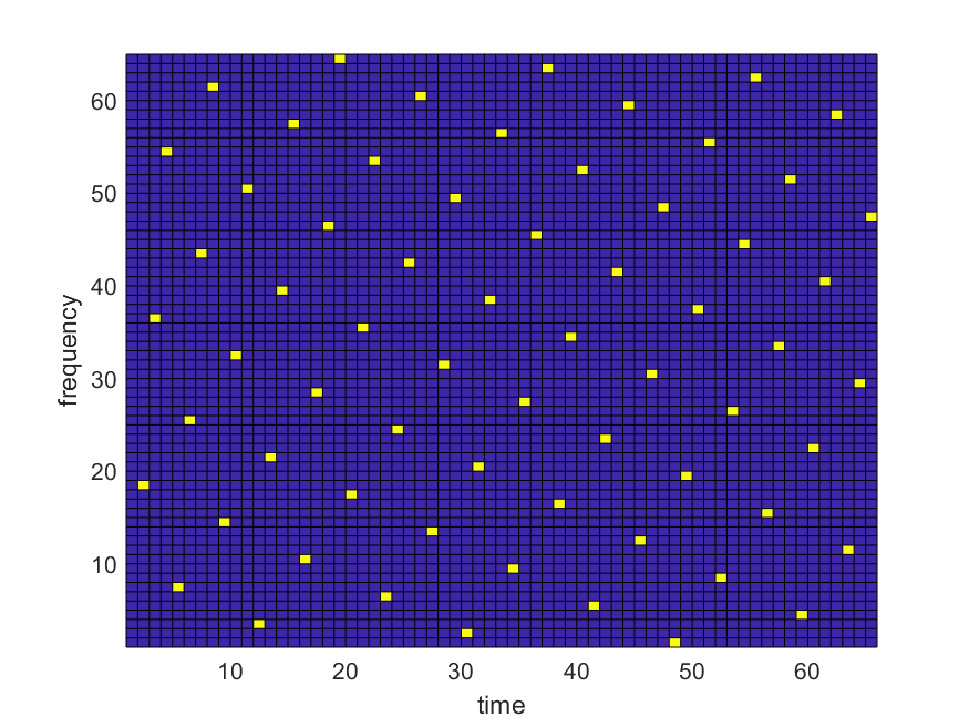
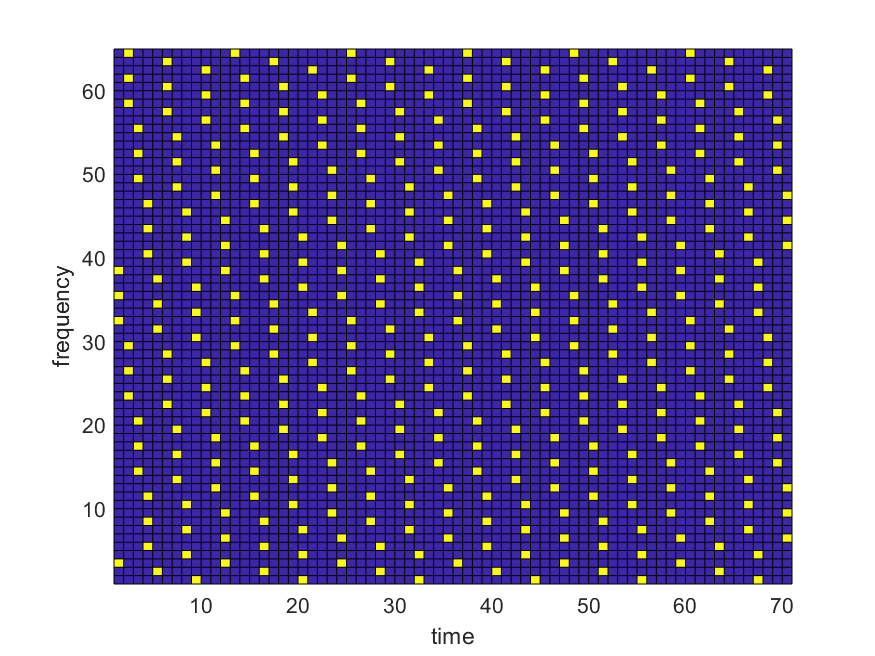
Figure 3: Generated pilot placement according to Algorithm 1 for $M^{\prime}=N^{\prime}=64$ and $P^{\prime}=1$ (left) and $P^{\prime}=6$ (right). The transmit frame size is $64\times 65$ (left) and $64\times 70$ (right).

Algorithm 1 Accordion pilot placement

1:Data frame size $(M^{\prime},N^{\prime})$ and pilots per row $P^{\prime}$.

2:Pilot indices $\mathcal{P}\subset\mathcal{I}$, transmit frame size $(M,N)$.

3:$M\leftarrow M^{\prime}$

4:$N\leftarrow N^{\prime}+P^{\prime}$

5:$\lambda\leftarrow\operatorname{round}(N/P^{\prime})$

6:$\displaystyle\mu_{\text{opt}}\leftarrow\operatorname*{argmax}_{\mu=0,\dots,\lambda-1}\ \min_{\ell=-\lambda,\dots,\lambda}\ell^{2}+(\lambda k_{\mu,\ell}+\mu\ell)^{2}$

7:       where $k_{\mu,\ell}$ as defined in 47.

8:$\mathcal{R}\leftarrow\left\{\operatorname{round}(\bar{n}N/P^{\prime}):\bar{n}=0,\dots,P^{\prime}-1\right\}$

9:$\mathcal{P}^{(0)}\leftarrow\varnothing$

10:for $\bar{m}=1,\dots,M$ do

11:     $\mathcal{R}^{(\bar{m})}\leftarrow\left(\mu\bar{m}+\mathcal{R}\right)\mod{N}$

12:     $\mathcal{P}^{(\bar{m})}\leftarrow\mathcal{P}^{(\bar{m}-1)}\cup\left\{(\bar{m},\bar{n}):\bar{n}\in\mathcal{R}^{(\bar{m})}\right\}$

13:end for

14:$\mathcal{P}\leftarrow\mathcal{P}^{(M)}$

VI Numerical simulations and results

In this section, we present the simulation setup and numerical results. We compare the performance of different linear precoding transformations and evaluate the proposed channel estimation scheme.

VI-A Numerical simulation setup

For the numerical evaluation, we choose a typical URLLC scenario in which a vehicle receives short-frame messages from a base station [10]. In this scenario, the vehicle has to reliably recover the transmitted bits from each frame. To do so, the channel is estimated and equalized on a per frame basis.

To evaluate pulse-shaped multicarrier systems in high-mobility scenarios, the right choice of the simulation setup is essential. In Table I, we list the selected simulation and system parameters. We use the geometric-statistical channel simulator QuaDRiGa to generate the channels [43]. To obtain doubly-dispersive channels, we update the channel samples generated by the simulator within the duration of one frame. The channel then becomes time-variant at higher velocities. We therefore configure the simulator to update the channel samples at a rate of $\nicefrac{{1}}{{B}}$=0.2 $\mu$s. For the channel model, we choose the 3GPP 38.901 UMi non line-of-sight (NLOS) model which takes $R$=58 multipaths into account. All together, the high sampling rate, the NLOS scenario, and high velocities allow us to obtain highly time-variant channels with our simulation setup.

To realize the pulse-shaped multicarrier system, we use LTFAT which provides a transceiver structure based on a polyphase implementation of filtering [44]. We choose a TF product of $TF=1.25$ to balance the trade-off between the signal to interference ratio and spectral efficiency [45]. In the TF domain, we design the short-frame to consist of $N=64$ time steps and $M=64$ frequency steps [14]. We use a bandwidth of $B=5$ MHz and a frame duration of $T_{f}=1$ ms. This results in a time step size of $T=16\,\mu$s and a frequency step size of $F=78.125$ kHz which are also referred to as symbol length and subcarrier spacing, respectively. At the Gabor filterbank, we utilize orthogonalized Gaussian-like pulses to synthetize and analyze the transmitted and received signal in the time domain, respectively. These pulses are generated by orthogonalizing a prototype pulse on a tight Gabor frame which is commonly referred to as $S^{-1/2}$-trick [34, 46]. These pulses are identical by construction, i.e., $\gamma=g$, and each pulse is orthogonal to its translations on the TF grid. From the channel simulator, we get 58 multipaths with 5120 time samples for each of them. The total length of these channel samples corresponds to the duration of one frame, i.e., $T_{f}$=1 ms. Then, we apply a time-varying convolution between the transmit signal and each multipath and obtain the superposition of all of them as received signal. To assure a cyclic convolution, we add a block cyclic prefix to the samples with appropriate length.

TABLE I: Simulation and system parameters

Parameter	Notation	Value/description
Carrier frequency	$f_{c}$	5.9 GHz
Bandwidth	$B$	5 MHz
Frame duration	$T_{f}$	1 ms
Time step size	$T$	16 $\mu$s
Frequency step size	$F$	78.125 kHz
Number of time steps	$N$	64
Number of frequency steps	$M$	64
Modulation scheme	-	QPSK
Time-frequency product	$TF$	1.25
Synthesis and analysis pulse	$\gamma$ = $g$	orthogonalized Gaussian-like
Channel simulator	-	QuaDRIGa v2.4.0 [43]
Channel model	-	3GPP 38.901 UMi NLOS

(a) Relative symbol mean square error

(b) Uncoded bit error rate

(c) Normalized maximal symbol-error deviation

Figure 4: Performance comparison of different linear precoding transformations at 12 dB SNR assuming full CSI of CMD.

(a) Uncoded BER using 256 pilot symbols

(b) Coded BER (convolutional hard-decision decoding at rate of $\nicefrac{{1}}{{3}}$ ) using 256 pilot symbols.

(c) Uncoded BER using 512 pilot symbols

(d) Coded BER (convolutional hard-decision decoding at rate of $\nicefrac{{1}}{{3}}$ ) using 512 pilot symbols.

Figure 5: BER as a function of the SNR for different channel estimation schemes at relative velocity of $\Delta v=200\,\nicefrac{{\text{km}}}{{\text{h}}}$.

VI-B Comparison of distinct linear precoding setups

We numerically investigate the impact of applying different linear precoding transformations to the data frame, the gained TF diversity, and how this gain depends on the size of precoded data frame. Let us therefore detail the distinct setups considered in this subsection. Since we focus on precoding, we only place data symbols into the TF frame and assume full CSI knowledge of the CMD at the receiver. The perfect CMD is used for MMSE equalization as detailed in (38). To precode the data frame, we apply the DSFT, FWHT and fast Fourier transform (FFT) each as a 1D and 2D transformation, and we consider random precoding and without precoding as well. In addition, we study setups in which we subdivide the TF frame into two, four, and eight sub-frames (SF) corresponding to SF-2, SF-4, and SF-8, respectively. Fig. 6 depicts the TF frame in which the three considered SF structures are shown. The data frame is divided by the number of SF into smaller data frames. Each is then separately precoded and mapped to the corresponding SF. The approach of using precoded SF is particularly interesting for URLLC, as it provides higher flexibility. For example, a vehicle can already process single SF to recover the transmitted bits before receiving the entire frame. From another perspective, the SF can be used in multiuser scenarios improving reliability and providing higher flexibly than OTFS. This however comes at a price. Recall that by applying precoding to the data symbols, we increase the reliability of modulation or in other words we gain TF diversity. This is due to the fact that equalization errors and self-interference are distributed over all symbols. By reducing the size of the precoded data frame, we also decrease the potential TF diversity. To measure the impact of TF diversity gain on the precoded symbols, let us use the normalized maximal symbol-error deviation (NMSED) as metric.

Figure 6: TF frame with three different sub-frames (SF) structures. SF-2 consist of two times N=32 and M=64 symbols, SF-4 of four times N=16 and M=64 symbols, and SF-8 of eight times N=8 and M=64 symbols. In each SF the data symbols are separately precoded.

In Fig. 4, we study the mean square error (MSE), the uncoded BER, the NMSED as a function of the velocity for all investigated setups. Fig. 4a depicts the relative symbol MSE and shows that it is the same for all setups. Fig. 4b shows that all precoding functions achieve the same low BER when applied to the entire TF frame. In particular, 1D and 2D precoding lead to the same BER performance. We observe in general significant performance gains of precoded data frames compared to data frames without precoding. In the case of SF, we can observe that the BER increases by approximately 3 to 4 dB for each subdivision of the TF frame. The reason behind this behaviour can be explained when looking at NMSED in Fig. 4c. The precoding ensures that the error energy from self-interference and equalization near zero-crossings of $\bm{h}$ are equally distributed across all symbols in the TF frame.

TABLE II: Overview of investigated channel estimator schemes

Estimator	Description
LMMSE	Standard LMMSE estimator with noise-awareness
SRH	Minimizing isotropic ($\alpha=\beta$) second deviate in (30)
SRH-NA	Minimizing isotropic second deviate in (30) with noise-awareness by using the relaxation parameter $\delta$
SRH-MA	Minimizing the anisotropic second deviate in (30) with mode-awareness by using the scaling parameter $\alpha$ and $\beta$
SRH-MNA	Combining both SRH-NA and SRH-MA
perfect CMD	Assuming full CSI of the CMD

VI-C Performance of channel estimation

Let us evaluate the performance of channel estimation in a linearly precoded multicarrier system which is shown in Fig. 2. We place both pilot and precoded data symbols into the TF frame. We utilize the FWHT to precode the data frame which offers reduced implementation complexity compared to DSFT precoding [47]. The choice of precoding is however arbitrary since any other linear transformation leads to the same TF diversity gain as shown in Section VI-B. The pilot symbols are placed according to Algorithm 1. We estimate the CMD and use MMSE equalization to revert the distortion incurred by doubly-dispersive channel. We study the proposed channel estimation scheme by solving the optimization problem in (30) in four different configurations and denote them as follows: smoothness regularized Hessian (SRH), smoothness regularized Hessian with noise-awareness (SRH-NA), smoothness regularized Hessian with mode-awareness (SRH-MA), and smoothness regularized Hessian with mode- and noise-awareness (SRH-MNA). This allows us to study the impact of taking noise-awareness as well as the mode-awarness into account. We detail the investigated estimators in Table II.

Fig. 5 depicts the uncoded and coded BER as function of SNR for different numbers of pilot symbols using convolutional hard-decision decoding at rate of $\nicefrac{{1}}{{3}}$ in the latter case. In Fig. 5a, we show the uncoded BER using 256 pilots. Fig. 5b illustrates that with coding an error-free transmission is only achieved for the perfect CMD, SRH-MNA, and SRH-MA estimators at a SNR of 10.5 dB, 12 dB, and 13 dB, respectively. For all remaining estimators, an error floor between $-35$ and $-38$ dB is reached. Fig. 5c depicts the uncoded BER when 512 pilot symbols are used. By doubling the number of pilot symbols to 512, the standard LMMSE estimator performance is improved. Fig. 5d illustrates that with coding an error-free transmission is only achieved for the perfect CMD, SRH-MNA, and SRH-MA estimator at a SNR of 10.5 dB, 11 dB, and 13.2 dB, respectively. For all remaining estimators, an error floor between $-46$ and $-48$ dB is reached. Fig. 7 shows the uncoded BER as a function of the number of pilot symbols at a SNR of 15 dB with a relative velocity between 100 and 400 $\nicefrac{{\text{km}}}{{\text{h}}}$.

VII Conclusions

We proposed a novel channel main diagonal estimator scheme which minimizes the energy of the second order derivatives. This scheme considered noise including self-interference power and the ratio of the channel spreading region for anisotropic regularization of the weighted Hessian matrix. The use of Tikhonov regularization allowed us to obtain an unconstrained least-squares problem where a closed form solution for each noise parameter exists and can be computed offline. We introduced a new pilot placement scheme that enables a more efficient use of resources and improved channel estimation. The numerical results showed that the proposed scheme allows an accurate channel estimation and equalization of received short-frame messages even in highly time-varying communication scenarios.

(a) Uncode BER at $\Delta v=100\,\nicefrac{{\text{km}}}{{\text{h}}}$

(b) Uncode BER at $\Delta v=200\,\nicefrac{{\text{km}}}{{\text{h}}}$

(c) Uncode BER at $\Delta v=400\,\nicefrac{{\text{km}}}{{\text{h}}}$

Figure 7: BER as a function of the number of pilots in NLOS vehicular scenarios at a SNR of 15 dB for distinct channel estimators.

Andreas Pfadler received the M.Sc. degree in Telecommunication Engineering with specialization in wireless communications from the Polytechnic University of Catalonia (UPC), Barcelona, Spain, in 2018. He is a communication expert and function developer for automated driving at Volkswagen Commercial Vehicles and is currently pursuing the Ph.D. degree in vehicular communications with the Technische Universität of Berlin, under the supervision of Prof. Dr.-Ing. S. Stanczak. He has been involved in several research projects as the European project 5GCroCo and the German national project 5G NetMobil. His research interests include antennas, signal processing, predictive quality of service, new waveforms and wave propagation.

Tom Szollmann received the M.Sc. degree in mathematics with specialization in functional analysis and probability theory from the Technical University of Berlin in 2021. He is currently pursuing the Ph.D. degree in data management of vehicular communication in the context of automated driving at Volkswagen Commercial Vehicles under the supervision of Prof. G. Caire Ph.D., from the Technical University of Berlin. His research interests include signal processing, wireless channel estimation, predictive quality of service and machine learning.

Peter Jung (Member IEEE, Member VDE/ITG) received the Dipl.-Phys. in high energy physics in 2000 from Humboldt University, Berlin, Germany, in cooperation with DESY Hamburg. Since 2001 he has been with the Department of Broadband Mobile Communication Networks, Fraunhofer Institute for Telecommunications, Heinrich-Hertz-Institut (HHI) and since 2004 with Fraunhofer German-Sino Lab for Mobile Communications. He received the Dr.-rer.nat (Ph.D.) degree in 2007 (on Weyl–Heisenberg representations in communication theory) at the Technical University of Berlin (TUB), Germany. P. Jung is working under DFG grants at TUB in the field of signal processing, information and communication theory and data science. In 2021 he was a visiting professor at TU Munich and associated with the Munich AI Future Lab (AI4EO). His current research interests are in the area compressed sensing, machine learning, time–frequency analysis, dimension reduction and randomized algorithms. He is giving lectures in compressed sensing, estimation theory and inverse problems.

SŁAWOMIR STAŃCZAK is Professor of Network Information Theory at the Technical University of Berlin and Head of the Wireless Communications and Networks Department at the Fraunhofer Heinrich Hertz Institute (HHI). Prof. Stanczak is co-author of two books and more than 200 peer-reviewed journal articles and conference papers in the field of information theory, wireless communications, signal processing, and machine learning. Prof. Stanczak received research grants from the German Research Foundation and the Best Paper Award from the German Society for Telecommunications in 2014. He was an associate editor of the IEEE Transactions on Signal Processing from 2012 to 2015 and chair of the ITU-T Focus Group on Machine Learning for Future Networks including 5G from 2017 to 2020. Since 2020 Prof. Stanczak is chairman of the 5G Berlin association and since 2021 he is coordinator of the projects 6G-RIC (Research & Innovation Cluster) and CampusOS.

References

- [1] A. Kousaridas, R. P. Manjunath, J. Perdomo, C. Zhou, E. Zielinski, S. Schmitz, and A. Pfadler, “QoS Prediction for 5G Connected and Automated Driving,” IEEE Commun. Mag., vol. 59, no. 9, 2021.
- [2] Z. Li, M. A. Uusitalo, H. Shariatmadari, and B. Singh, “5G URLLC: Design challenges and system concepts,” in 2018 15th int. symposium on wireless commun. systems (ISWCS), pp. 1–6, IEEE, 2018.
- [3] S. Euler, A. Pfadler, L. F. Ferreira, and H. Zhao, “Spectrum Needs of Cooperative, Connected and Automated Mobility,” in 2021 IEEE 93rd Veh. Technol. Conf. (VTC2021-Spring), pp. 1–6, 2021.
- [4] P. Jung and G. Wunder, “On Time-Variant Distortions in Multicarrier with Application to Frequency Offsets and Phase Noise,” IEEE Trans. on Commun., vol. 53, pp. 1561–1570, sep 2005.
- [5] T. Wang, J. G. Proakis, E. Masry, and J. R. Zeidler, “Performance degradation of OFDM systems due to Doppler spreading,” IEEE Trans. on Wireless Commun., vol. 5, no. 6, 2006.
- [6] R. Hadani, S. Rakib, M. Tsatsanis, A. Monk, A. J. Goldsmith, A. F. Molisch, and R. Calderbank, “Orthogonal time frequency space modulation,” in 2017 IEEE Wireless Commun. and Netw. Conf. (WCNC), pp. 1–6, IEEE, 2017.
- [7] P. Raviteja, K. T. Phan, and Y. Hong, “Embedded pilot-aided channel estimation for OTFS in delay–Doppler channels,” IEEE Trans. on Veh. Technol., vol. 68, no. 5, pp. 4906–4917, 2019.
- [8] P. Raviteja, Y. Hong, E. Viterbo, and E. Biglieri, “Practical pulse-shaping waveforms for reduced-cyclic-prefix OTFS,” IEEE Trans. on Veh. Technol., vol. 68, no. 1, pp. 957–961, 2018.
- [9] A. Nimr, M. Chafii, M. Matthe, and G. Fettweis, “Extended GFDM Framework: OTFS and GFDM Comparison,” in 2018 IEEE Global Commnun. Conf. (GLOBECOM), pp. 1–6, 2018.
- [10] A. Pfadler, P. Jung, and S. Stanczak, “Pulse-Shaped OTFS for V2X Short-Frame Communication with Tuned One-Tap Equalization,” in WSA 2020; 24rd Int. ITG Workshop on Smart Antennas, pp. 1–6, VDE, 2020.
- [11] L. Gaudio, G. Colavolpe, and G. Caire, “OTFS vs. OFDM in the Presence of Sparsity: A Fair Comparison,” IEEE Trans. on Wireless Commun., vol. 21, no. 6, pp. 4410–4423, 2021.
- [12] P. Raviteja, K. T. Phan, Y. Hong, and E. Viterbo, “Interference cancellation and iterative detection for orthogonal time frequency space modulation,” IEEE Trans. on Wireless Commun., vol. 17, no. 10, pp. 6501–6515, 2018.
- [13] A. Pfadler, P. Jung, T. Szollmann, and S. Stanczak, “Pulse-Shaped OTFS over Doubly-Dispersive Channels: One-Tap vs. Full LMMSE Equalizers,” in 2021 IEEE Int. Conf. on Commun. Workshops (ICC Workshops), pp. 1–6, 2021.
- [14] A. Pfadler, T. Szollmann, P. Jung, and S. Stanczak, “Leakage suppression in pulse-shaped otfs delay-doppler-pilot channel estimation,” IEEE Wireless Commun. Lett., pp. 1–1, 2022.
- [15] R. M. Augustine and A. Chockalingam, “Interleaved time-frequency multiple access using otfs modulation,” in 2019 IEEE 90th Veh. Technol. Conf. (VTC2019-Fall), pp. 1–5, 2019.
- [16] A. Thomas, K. Deka, P. Raviteja, and S. Sharma, “Convolutional Sparse Coding based Channel Estimation for OTFS-SCMA in Uplink,” IEEE Trans. on Commun., pp. 1–1, 2022.
- [17] T. Zemen, M. Hofer, D. Loeschenbrand, and C. Pacher, “Iterative detection for orthogonal precoding in doubly selective channels,” in 2018 IEEE 29th Annual Int. Symp. on Pers., Indoor and Mobile Radio Commun. (PIMRC), pp. 1–7, IEEE, 2018.
- [18] P. Bello, “Characterization of Randomly Time-Variant Linear Channels,” IEEE Trans. on Commun. Syst., vol. 11, no. 4, pp. 360–393, 1963.
- [19] J. Seo, S. Jang, J. Yang, W. Jeon, and D. K. Kim, “Analysis of Pilot-Aided Channel Estimation with Optimal Leakage Suppression for OFDM Systems,” IEEE Trans. Lett., vol. 14, no. 9, pp. 809–811, 2010.
- [20] X. Xiong, B. Jiang, X. Gao, and X. You, “DFT-Based Channel Estimator for OFDM Systems with Leakage Estimation,” IEEE Trans. Lett., vol. 17, no. 8, pp. 1592–1595, 2013.
- [21] P. Hoeher, S. Kaiser, and P. Robertson, “Two-dimensional pilot-symbol-aided channel estimation by wiener filtering,” in 1997 IEEE int. conf. on acoustics, speech, and signal processing, vol. 3, IEEE, 1997.
- [22] V. Savaux and Y. Louët, “LMMSE channel estimation in OFDM context: a review,” IET Signal Processing, vol. 11, no. 2, pp. 123–134, 2017.
- [23] G. Taubock, F. Hlawatsch, D. Eiwen, and H. Rauhut, “Compressive estimation of doubly selective channels in multicarrier systems: Leakage effects and sparsity-enhancing processing,” IEEE J. of Sel. Topics in Signal Proces., vol. 4, no. 2, pp. 255–271, 2010.
- [24] R. Beinert, P. Jung, G. Steidl, and T. Szollmann, “Super-resolution for doubly-dispersive channel estimation,” Sampling Theory, Signal Processing, and Data Analysis, vol. 19, no. 2, 2021.
- [25] O. K. Rasheed, G. D. Surabhi, and A. Chockalingam, “Sparse Delay-Doppler Channel Estimation in Rapidly Time-Varying Channels for Multiuser OTFS on the Uplink,” in 2020 IEEE 91st Veh. Technol. Conf. (VTC2020-Spring), pp. 1–5, 2020.
- [26] L. Zhao, W.-J. Gao, and W. Guo, “Sparse Bayesian Learning of Delay-Doppler Channel for OTFS System,” IEEE Commun. Lett., vol. 24, no. 12, pp. 2766–2769, 2020.
- [27] Z. Wei, W. Yuan, S. Li, J. Yuan, and D. W. K. Ng, “Off-grid channel estimation with sparse bayesian learning for otfs systems,” IEEE Trans. on Wireless Commun., pp. 1–1, 2022.
- [28] F. Liu, Z. Yuan, Q. Guo, Z. Wang, and P. Sun, “Message Passing-Based Structured Sparse Signal Recovery for Estimation of OTFS Channels With Fractional Doppler Shifts,” IEEE Trans. on Wireless Commun., vol. 20, no. 12, pp. 7773–7785, 2021.
- [29] L. Bernadó, T. Zemen, F. Tufvesson, A. F. Molisch, and C. F. Mecklenbräuker, “The (in-) validity of the WSSUS assumption in vehicular radio channels,” in 2012 IEEE 23rd Int. Symposium on Personal, Indoor and Mobile Radio Commun. - (PIMRC), pp. 1757–1762, 2012.
- [30] W. Kozek, “Matched Weyl-Heisenberg expansions of nonstationary environments,” 1996.
- [31] W. Kozek and A. F. Molisch, “Nonorthogonal pulseshapes for multicarrier communications in doubly dispersive channels,” IEEE J. on Sel. Areas in Commun., vol. 16, pp. 1579–1589, Oct 1998.
- [32] K. Liu, T. Kadous, and A. M. Sayeed, “Orthogonal time-frequency signaling over doubly dispersive channels,” IEEE Trans. on Inf. Theory, vol. 50, no. 11, pp. 2583–2603, 2004.
- [33] P. Jung, Weyl–Heisenberg Representations in Communication Theory. PhD thesis, Technical University Berlin, 2007. https://depositonce.tu-berlin.de/handle/11303/1948.
- [34] P. Jung and G. Wunder, “WSSUS pulse design problem in multicarrier transmission,” IEEE Trans. on Commun., vol. 55, no. 9, 2007.
- [35] T. Thaj and E. Viterbo, “Orthogonal time sequency multiplexing modulation,” in 2021 IEEE Wireless Trans. and Netw. Conf. (WCNC), pp. 1–7, 2021.
- [36] M. Zhang, F. Wang, X. Yuan, and L. Chen, “2D Structured Turbo Compressed Sensing for Channel Estimation in OTFS Systems,” in 2018 IEEE Int. Conf. on Commun. Syst. (ICCS), pp. 45–49, 2018.
- [37] W. Shen, L. Dai, J. An, P. Fan, and R. W. Heath, “Channel Estimation for Orthogonal Time Frequency Space (OTFS) Massive MIMO,” IEEE Trans. on Signal Processing, vol. 67, no. 16, 2019.
- [38] Z. Wei, W. Yuan, S. Li, J. Yuan, and D. W. K. Ng, “Transmitter and Receiver Window Designs for Orthogonal Time-Frequency Space Modulation,” IEEE Trans. on Commun., vol. 69, no. 4, 2021.
- [39] D. G. Luenberger, Optimization by vector space methods. John Wiley & Sons, 1997.
- [40] P. Jung, W. Schuele, and G. Wunder, “Robust path detection for the LTE downlink based on compressed sensing,” in 14th Int. OFDM-Workshop, Hamburg, 2009.
- [41] S. Boyd, S. P. Boyd, and L. Vandenberghe, Convex optimization. Cambridge university press, 2004.
- [42] G. H. Golub, P. C. Hansen, and D. P. O’Leary, “Tikhonov regularization and total least squares,” SIAM journal on matrix analysis and applications, vol. 21, no. 1, pp. 185–194, 1999.
- [43] S. Jaeckel, L. Raschkowski, K. Börner, and L. Thiele, “QuaDRiGa: A 3-D multi-cell channel model with time evolution for enabling virtual field trials,” IEEE Trans. on Antennas and Propag., vol. 62, no. 6, 2014.
- [44] Z. Průša, P. L. Søndergaard, N. Holighaus, C. Wiesmeyr, and P. Balazs, “The Large Time-Frequency Analysis Toolbox 2.0,” in Sound, Music, and Motion, LNCS, pp. 419–442, Springer Int. Publishing, 2014.
- [45] G. Matz, D. Schafhuber, K. Grochenig, M. Hartmann, and F. Hlawatsch, “Analysis, optimization, and implementation of low-interference wireless multicarrier systems,” IEEE Trans. on Wireless Commun., vol. 6, no. 5, pp. 1921–1931, 2007.
- [46] A. Sahin, I. Guvenc, and H. Arslan, “A Survey on Multicarrier Communications: Prototype Filters, Lattice Structures, and Implementation Aspects,” IEEE Trans. Surveys & Tutorials, vol. 16, no. 3, 2014.
- [47] R. Bomfin, M. Chafii, A. Nimr, and G. Fettweis, “A Robust Baseband Transceiver Design for Doubly-Dispersive Channels,” IEEE Trans. on Wireless Commun., vol. 20, no. 8, pp. 4781–4796, 2021.