New and simplified manual controls for projection and slice tours, with application to exploring classification boundaries in high dimensions

Abstract

This paper describes new user controls for examining high-dimensional data using low-dimensional linear projections and slices. A user can interactively change the contribution of a given variable to a low-dimensional projection, which is useful for exploring the sensitivity of structure to particular variables. The user can also interactively shift the center of a slice, for example, to explore how structure changes in local subspaces. The Mathematica package as well as example notebooks are provided, which contain functions enabling the user to experiment with these new manual controls, with one specifically for exploring regions and boundaries produced by classification models. The advantage of Mathematica is its linear algebra capabilities, and interactive cursor location controls. Some limited implementation has also been made available in the R package tourr.

1 Introduction

From a statistical perspective 3D is a rare data dimension, so unlike in most 3D rotation computer graphics applications, the more useful methods for data analysis need to work for arbitrary dimension. A good approach is to show projections from an arbitrary dimensional space to create dynamic data visualizations called tours. Tours involve views of high-dimensional ($p$) data with low-dimensional ($d$) projections. In his original paper on the grand tour, Asimov (1985) provided several algorithms for tour paths that could theoretically show the viewer the data from all sides. Prior to Asimov’s work, there were numerous preparatory developments including Fisherkeller, Friedman, and Tukey (1974)’s PRIM-9. PRIM-9 had user-controlled rotations on coordinate axes, allowing one to manually tour through low-dimensional projections. (A video illustrating the capabilities is available through video library of ASA Statistical Graphics Section (2022).) Steering through all possible projections is impossible, unlike Asimov’s tours which allows one to quickly see many, many different projections. After Asimov there have been many tour developments, which are summarized in Lee et al. (2021).

One such direction of work develops the ideas from PRIM-9, to provide manual control of a tour. Cook and Buja (1997) describe controls for 1D (or 2D) projections, respectively in a 2D (or 3D) manipulation space, allowing the user to select any variable axis, and rotate it into, or out of, or around the projection through horizontal, vertical, oblique, radial or angular changes in value. Spyrison and Cook (2020) refined this algorithm and implemented it to generate radial tour animation sequences.

Manual controls are especially useful for assessing sensitivity of structure to particular elements of the projection. There are many places where it is useful. In exploratory data analysis, where one sees clusters in a projection, one may ask whether some variables can be removed from the projection without affecting the clustering. For interpreting models, one can reduce or increase a variable’s contribution to examine the variable importance. Having the user interact with a projection is extremely valuable for understanding high-dimensional data. However, these algorithms have two problems: (1) the pre-processing of creating a manipulation space overly complicates the algorithm, (2) extending to higher dimensional control is difficult.

Another potentially useful manual control, is to allow the user to choose the position of the center of a slice. The slice tour was introduced in Laa, Cook, and Valencia (2020). It operates by converting the projection plane into a slice, by removing or de-emphasizing points that are further than a fixed orthogonal distance from the plane. The projection plane is usually thought of as passing through the center of the data. Manual control would allow the user to change the position of the center point, by shifting it along a coordinate axis, while keeping the orientation of the projection plane fixed. The purpose would be to explore how or if the shape of the data, in the space orthogonal to the projection, changes as one gets away from the center. It would also allow the user to interactively decide on the thickness of the slice.

This paper explains the new manual controls for projection and slice tours. The next section describes the new algorithm for manual control, for both projections and slices. The use of these methods is illustrated to compare and contrast boundaries constructed by different classifiers. The software section describes a mathematica package that is used for the application, and describes the interactive environment that would be desirable within R as new technology becomes available. The paper is accompanied by an appendix with more details and adjustments to the manual controls, and three Mathematica notebooks that can be used to reproduce the application.

2 How to construct a manual tour

A manual tour allows the user to alter the coefficients of one (or more) variables contributing to a $d$ dimensional projection. The initial ingredients are an orthonormal basis ($A_{p\times d}$) defining the projection of the data, and a variable id ($m\in\{1,...,p\}$) specifying which coefficient will be changed. A method to update the values of the component ($m^{th}$ row of $A_{p\times d}$) of the controlled variable $V_{m}$ is then needed.

2.1 Existing methods

The methods for updating component values in Cook and Buja (1997) (and utilized in Spyrison and Cook (2020)) are prescribed primarily for a 2D projection, to take advantage of (then) newly developed 3D trackball controls made available for computer gaming. The first step was to construct a 3D manipulation space from a 2D projection. In this space, the coefficient of the controlled variable ranges between -1 and 1. Movements of a cursor are recorded and converted into changes in the values of $V_{m}$ thus changing the displayed 2D projection. The algorithm also provided constraints to horizontal, vertical, radial or angular motions only. The construction of the manipulation space overly complicates the manual controls, especially when considering possible techniques that will apply to arbitrary $d$.

2.2 A new simpler and broadly applicable approach

The new approach emerged from experiments on the tour using the linear algebra capabilities, and relatively new interactive graphics interface, available in Mathematica (Wolfram Research, Inc. 2022). The components corresponding to $V_{m}$ are directly controlled by cursor movement, which updates row $m$ of $A$. The updated matrix is then orthonormalised.

2.2.1 Algorithm

1. Provide $A$, and $m$. (Note that $m$ could also be automatically chosen as the component that is closest to the cursor position.)

2. Change values in row $m$, for example, if $d=2$ gives

   $$A^{*}=[\boldsymbol{a}^{*}_{1}~{}\boldsymbol{a}^{*}_{2}]=\left[\begin{array}[]{cc}a_{11}&a_{12}\\ \vdots&\vdots\\ a^{*}_{m1}&a^{*}_{m2}\\ \vdots&\vdots\\ a_{p1}&a_{p2}\end{array}\right].$$

   A large change in these values would correspond to making a large jump from the current projection. Small changes would correspond to tracking a cursor, making small jumps from the current projection.

3. Orthonormalise $A^{*}$, using Gram-Schmidt.

   1. Normalise $\boldsymbol{a}^{*}_{1}$ and $\boldsymbol{a}^{*}_{2}$.

   2. $\boldsymbol{a}^{*}_{2}=\boldsymbol{a}^{*}_{2}-(\boldsymbol{a}^{*}_{1}\cdot\boldsymbol{a}^{*}_{2})\boldsymbol{a}^{*}_{1}$.

This algorithm will produce the changes to a projection as illustrated in Figure 1. The controlled variable, $V_{m}$, corresponds to the black line, and sequential changes to row $m$ of $A$ can be seen to roughly follow a specified position (orange dot). Changes in the other components happen as a result of the orthonormalisation, but are uncontrolled.

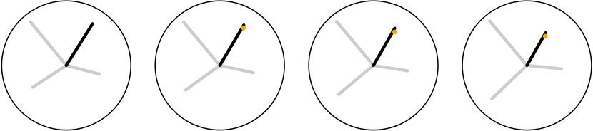
Figure 1: Sequence of projections where contribution of one variable is controlled (black) is changed using unconstrained orthonormalisation. The dot (orange) indicates the chosen values for the controlled variable. It can be seen that the actual axis does not precisely match the chosen position, but it is close.

2.3 Refinements to enforce exact position

The problem with the new simple method is that it is not faithful to the precise values for $V_{m}$ because the orthonormalisation will change them. Even though these changes are for the most part imperceptible, one may wish to avoid them and there are numerous ways that this can be enforced, a few are detailed in the Appendix. These primarily differ in how the remaining variables are adjusted during orthonormalisation.

2.4 Manual control for slices

To better explore the space we combine the manual controls for the projection with manual controls for slicing. A slice is a section of the data that is defined by a projection, a center point that is anchoring it in the high-dimensional space and the slice thickness $h$ (Laa, Cook, and Valencia 2020). A data point is inside the slice if its orthogonal distance from the projection plane (passing through the center point) is below the thickness $h$. This orthogonal distance is computed in terms of the component that is normal on the projection plane. For $\mathbf{x}_{i}$ a $p$ dimensional data point and $\mathbf{c}$ the center point (in the same $p$ dimensional space) we compute the orthogonal distance as

$$v_{i}^{2}=||\mathbf{x}_{i}^{\prime}-\mathbf{c}^{\prime}||^{2}=\mathbf{x}_{i}^{\prime 2}+\mathbf{c}^{\prime 2}-2\mathbf{x}_{i}^{\prime}\cdot\mathbf{c}^{\prime},$$ (1)

with $\mathbf{c}^{\prime}=\mathbf{c}-(\mathbf{c}\cdot\mathbf{a}_{1})\mathbf{a}_{1}-(\mathbf{c}\cdot\mathbf{a}_{2})\mathbf{a}_{2}$, $\mathbf{x}_{i}^{\prime}=\mathbf{x}_{i}-(\mathbf{x}_{i}\cdot\mathbf{a}_{1})\mathbf{a}_{1}-(\mathbf{x}_{i}\cdot\mathbf{a}_{2})\mathbf{a}_{2}$ and $\mathbf{a}_{k},k=1,2(=d)$ denoting the columns of the projection matrix, $\mathbf{A}=(\mathbf{a}_{1},\mathbf{a}_{2})$.

2.4.1 Shifting the center

A natural starting point is to place $\mathbf{c}$ in the center of the data distribution, but shifting it away from the mean can provide additional insights. In the case of a single orthogonal direction on the projection plane we can pick a sequence of center points $\mathbf{c}$ in steps along that direction to move the slice and fully cover the data space. This no longer works in higher-dimensional spaces, and we can think of picking one direction and shifting the slice along the component orthogonal to the projection plane.

2.4.2 Changing the thickness

In addition it is also useful to interactively change the slice thickness $h$ (also called the slice radius), in particular to find the preferred value for exploring the input data. For guidance the estimates of the number of points inside the slice as a function of the original sample size $N$ and the number of dimensions $p$ from Laa et al. (2022) can be used: in case of a uniform distribution inside a sphere of radius $R$ a slice with thickness $h$ will contain $N_{S}$ points, with

$$N_{S}(h,p,R,N)=\frac{N}{2}\left(\frac{h}{R}\right)^{p-2}\left(p-(p-2)\left(\frac{h}{R}\right)^{2}\right).$$ (2)

3 Software

The implementation of the manual tour as suggested here requires the visualization of the current projection in terms of an axis display (see Figure 1 for an example). This display should be able to track the mouse position and adjust the projection based on the user selection. The user can select one axis (corresponding to one variable) by clicking on it, and then adjust the position of that axis by dragging it during the click event. In practice the closest axis will be selected, and the dragging results in tracking of the mouse position which will update the projection in small steps, such that no further interpolation is required.

The interactions in the axis display need to be mapped back onto the current projection matrix, which will then be orthonormalized before feeding back into the axis display. A second, linked display shows the projected data in sync with the updates from the axis display.

In addition, we also want to be able to look at slices of the data and select slicing parameters interactively. Here we have implemented a switch to change between projection and slice view, a slider that adjusts the slice thickness $h$ (dubbed height in the Mathematica package) and a numeric input to specify the center point $c$ explicitly. The display will update based on these inputs, in particular the view will jump to a new slice when $c$ is changed (though an interpolation might also be useful).

One might implement such an interactive interface via R Shiny, but in particular the tracking of the mouse position in small increments might pose a challenge. Here we found the dynamic graphics interface from Mathematica to be especially useful. In the following we first describe the relevant Mathematica functionalities and how they were used in the implementation, followed by a brief sketch of how the new approaches are implemented in the tourr package. There is hope that better interactivity will be available for R soon, which might allow for implementation of the techniques developed in Mathematica.

3.1 Mathematica package

Mathematica provides much utility and versatility, such as inbuilt data visualization, data manipulation and analysis, dynamic functionality, and symbolic and numeric computation. Most of this inbuilt functionality is user-friendly and described in the Mathematica documentation; typically, numerous examples are provided within the documentation, and some possible issues are outlined there.

Importantly for our work, it is relatively simple to create dynamic objects via the inbuilt commands Manipulate or DynamicModule. Control objects, such as sliders, locator panes, and input fields, can then be used on dynamic variables, and when there is a change in the dynamic variable the dynamic objects which contain that variable will be updated. This is the essential ingredient for this implementation of the manual tour.

The most relevant inbuilt Mathematica function for our purpose is the LocatorPane. This creates a region on the screen where the position of the mouse is captured and then converted to input that updates the graphics functions, enabling the manual navigation of the tour.

The examples presented in the application section below (and attached in notebook format in the supplementary material) all use our primary new function, SliceDynamic. This function typically accepts grouped data in the form of a matrix where the second last column details the name of the group and the last column details the group index (which can be one if there is only one group). After specifying the initial slice thickness and the slice range, the user is presented with an interactive display in which the control objects appear on the left and the slice visualization appears on the right. The user can change the orientation of the slice via the locator pane, which changes the projection matrix; a slider controls the slice thickness; and there is an input field, which changes the slice center. The user can also change the appearance of the plot by zooming into the center or changing the point size with the sliders provided. It is worth noting that this zoom works best with data that has been centered and scaled. The projected data can be displayed to contrast it with the slice by ticking a box. The explicit projection matrix can also be displayed via another checkbox. This is especially useful when we wish to import a projection that was identified as interesting in the manual exploration into a later study, as shown in the applications below.

Details about the implementation and usage instructions are given in the Appendix.

3.2 Extensions to the R package tourr

The R package tourr (Wickham et al. 2011) provides numerous types of tours. An additional function, radial_tour() has been constructed that will generate a sequence of projections that will decrease the coordinates for $V_{m}$ to $\boldsymbol{0}$ and back to the original values. It is applicable for any projection dimension, $d$. Changing slice center manually can be accomplished with the new function, manual_slice(). This changes the value of the center point ($\mathbf{c}$) of the slice, along a selected variable axis. It slices from the center of the data out to one side, back to the center, out to the opposite side, and then back to the center. The appendix contains a discussion of a possible visual guide for the slice center location.

4 Application

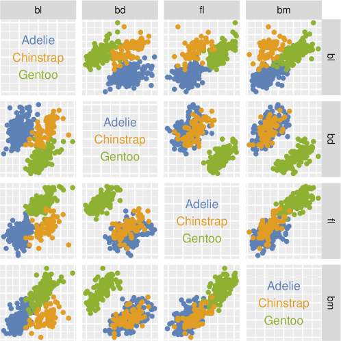
Figure 2: Scatterplot matrix of the (standardised) penguins data. The three species are reasonably different in size, with Gentoo distinguised from the other two on body depth relative to flipper length and body mass.

To illustrate the usefulness of the manual controls we use the 4D penguins data (Horst, Hill, and Gorman 2020) and look at classification models following Wickham, Cook, and Hofmann (2015). We will show how classification boundaries can be explored and better understood on projections and slices through 4D space. Figure 2 shows a scatterplot matrix of this data. There are four variables (bl = bill_length_mm, bd = bill_depth_mm, fl = flipper_length_mm, bm = body_mass_g) measuring the size of the penguins from three species (Adelie, Chinstrap and Gentoo). The scatterplot matrix shows that the three species appear to be likely separable, and that at least the Gentoo can be distinguished from the other two species when bd is paired with fl or bm. The steps for exploring boundaries in this example are as follows:

1. Build your classification model.

2. Predict the class for a dense grid of values covering the data space.

3. Examine projections, using a manual tour so that the contribution of any variable is controlled.

4. Slice through the center, to explore where the boundaries will likely meet.

5. Move the slice by changing the center in the direction of a single variable to explore the extent of a boundary for a single group relative to a variable.

4.1 Constructing the 4D prediction regions

We use the classifly package (Wickham 2022) to generate predictions across the 4D cube spanned by the data, with two classification models: linear discriminant analysis (LDA) and random forest (RF). Both the data and the model points in the grid are centered and scaled (standard deviation $=1$).

4.2 Exploring projections manually

We start by exploring the projections of the model prediction. Figure 3 summarizes the process. Rotating manually the view, we can visualize the location of predictions for each of the three species, and also get a sense of the difference between the two models. To illustrate this difference, we have manually rotated the projection for the RF model (left plot) to identify a view that shows the non-linear but block-type structure that is typical of this type of model. This particular projection ($A_{1}$) is exported so that it can later be used to show the LDA model (middle plot) and the actual data (right plot). What can be seen is the linearity of the LDA model, where the boundaries are linear and oblique to the variable axes. And, interestingly, this particular projection of the original data shows very distinct clusters of the three species. That means, the obscuring of the boundaries between groups for both of the models is driven by what is happening in the orthogonal space to the plane of the selected projection.

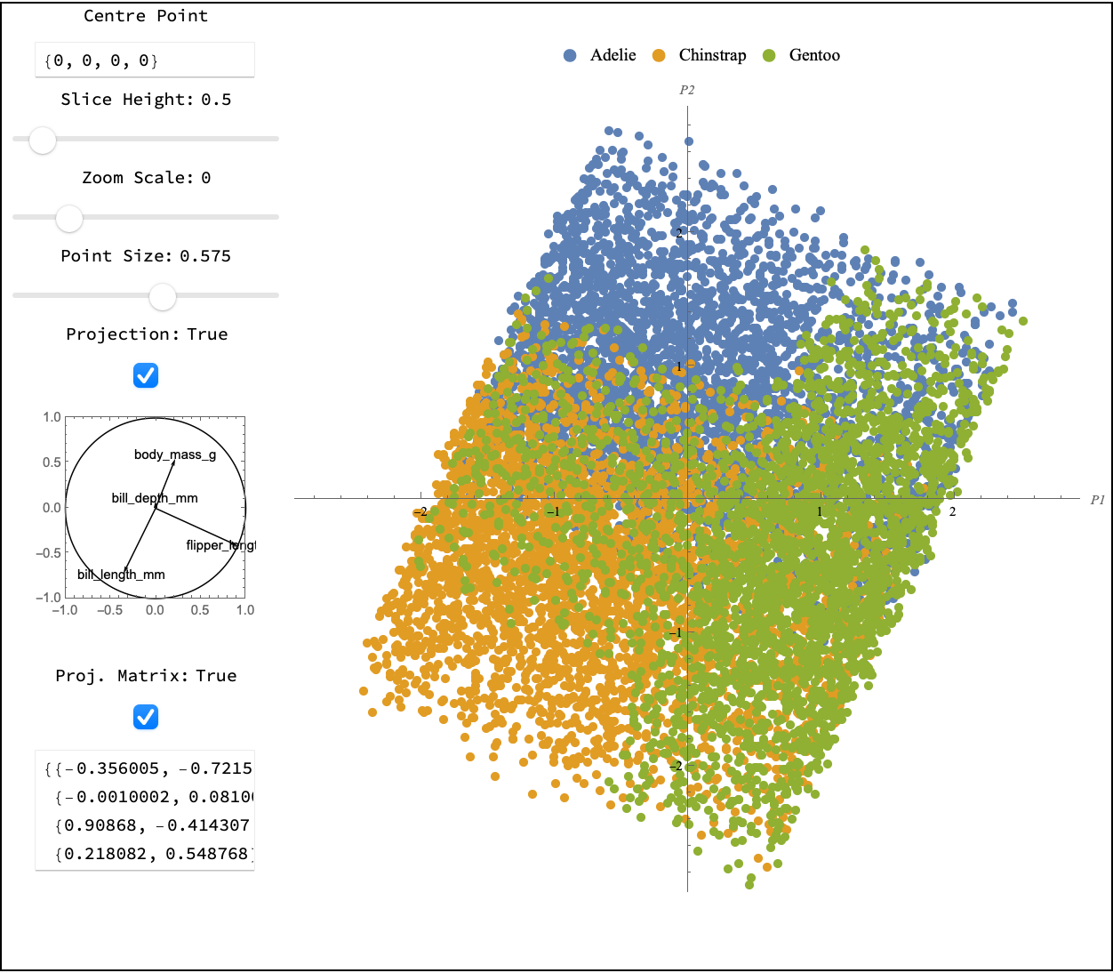
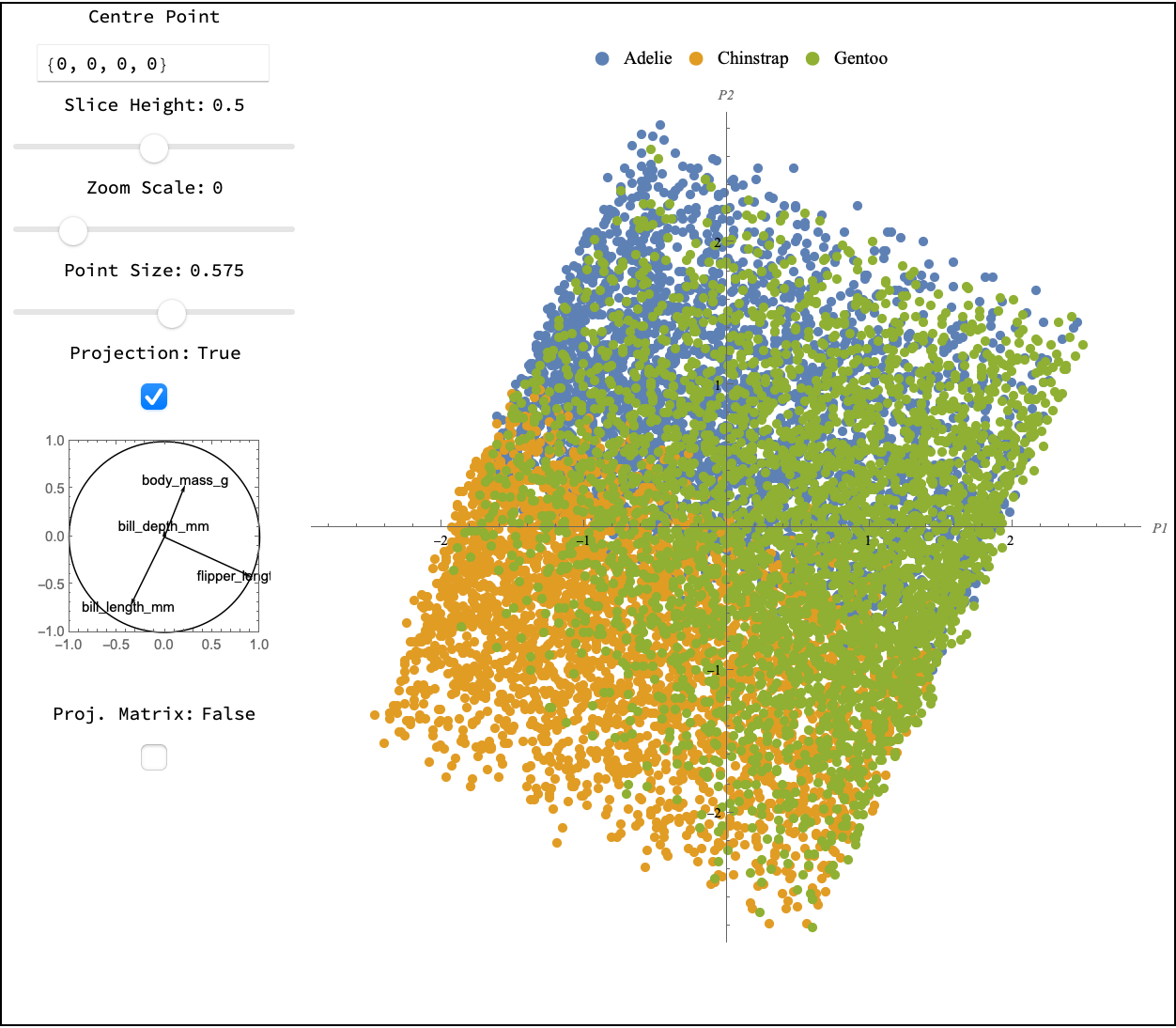
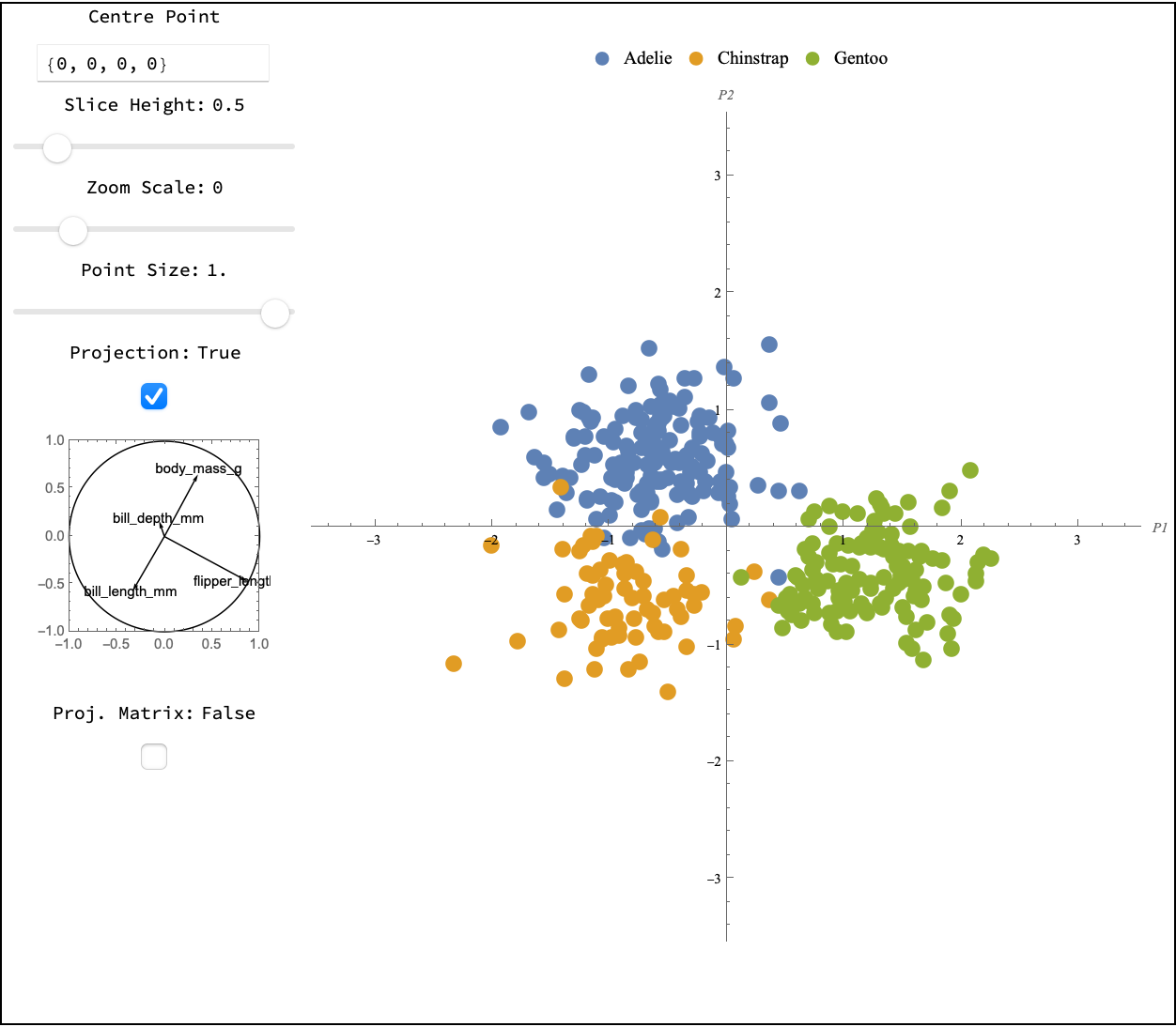
Figure 3: Projection identified using the manual tour, because it reveals an interesting structure in the predictions from the RF model (left). We can clearly see a block structure, while the LDA model (middle) produces linear boundaries. The three groups are nicely separated in this projection of the data (right).

This example can be reproduced with the code in penguins_exploring_manually.nb and a run through is shown in the video at https://vimeo.com/747585410.

4.3 Slicing through the center

We now continue the investigation by slicing orthogonally to the projection $A_{1}$. For both models we look at a thin ($h=0.5$) slice through the center, $\mathbf{c}^{0}=(0,0,0,0)$. At first we explore how changing the projection away from $A_{1}$ can help with understanding the boundary better. For our example, notice that $A_{1}$ does not contain any contribution from the second variable (bd), so we will first rotate this variable into the view.

Figure 4 shows snapshots of the exploration. The top row is the initial projection ($A_{1}$ and $\mathbf{c}^{0}$), and the bottom row is a later projection containing more of bd (new projection $A_{2}$ while keeping the center fixed at $\mathbf{c}^{0}$). The columns correspond to the two models, with RF on the left and LDA on the right.

Both models have some overlap at the center for the thin slice based on $A_{1}$ (despite the small value for $h$). The second slice (based on $A_{2}$) mostly resolves this overlap and reveals the primary differences between the models. The boundary between Adelie (blue) and Chinstrap (yellow) is very similar for both models. The boundary between Chinstrap and Gentoo (green) is where they differ.

The RF is almost straight in this view, as something we might expect from a tree model where splitting occurs on single variables only. However, it is straight in a combination of the second and third variable (bd and fl). By examining the scatterplot matrix, we can understand how this boundary was built: on each of bd and fl it is possible to cut on a value where most of the Gentoo penguins are different from the other two species for any tree, and likely only one is needed. Thus the forest construction is providing a sample of trees that use one variable or the other variable to split, producing the blocky boundary on the combination of the two.

In contrast, the LDA boundary has an oblique split between the two, and roughly divides the space into three similarly sized areas. It is almost like a textbook illustration of how LDA works for two variables (2D) where by assuming the clusters have equal variance-covariance, it places a boundary half-way between the group means.

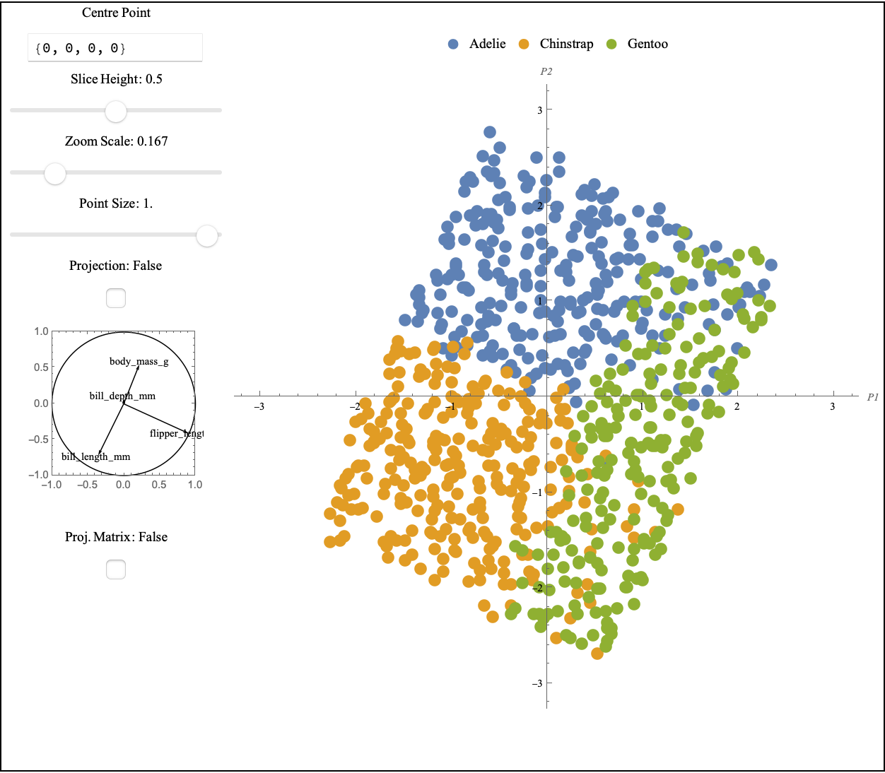
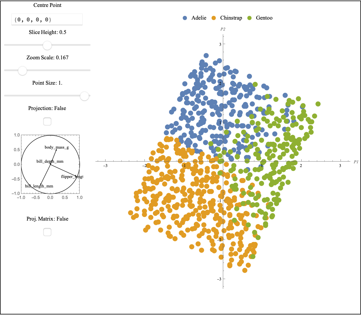
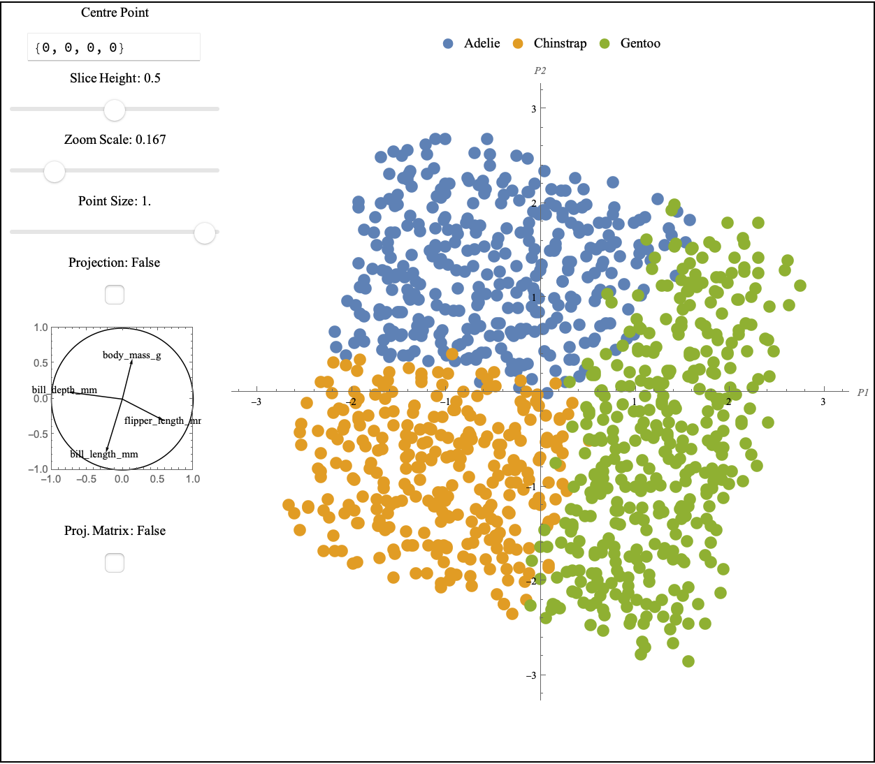
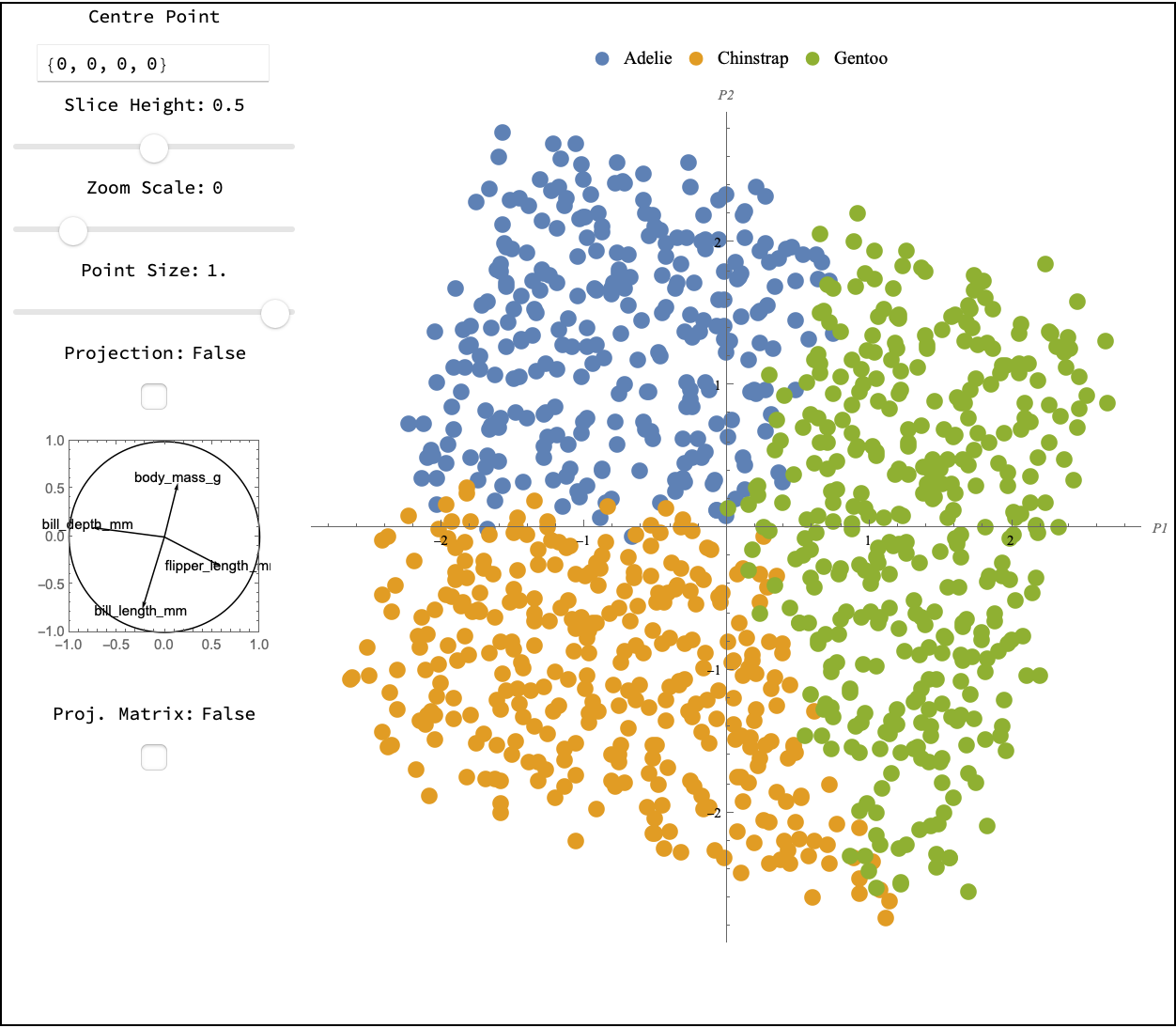
Figure 4: Comparing slices based on two projections $A_{1}$ (top row) and $A_{2}$ (bottom row), for the two models RF (left) and LDA (right). With $A_{1}$ we see two groups overlap (green - Gentoo with yellow - Chinstrap), while the rotation to $A_{2}$ results in clear boundaries inside the slice. The boundary between Adelie (blue) and Chinstrap (yellow) is similar for both models but very different between Chinstrap and Gentoo (green).

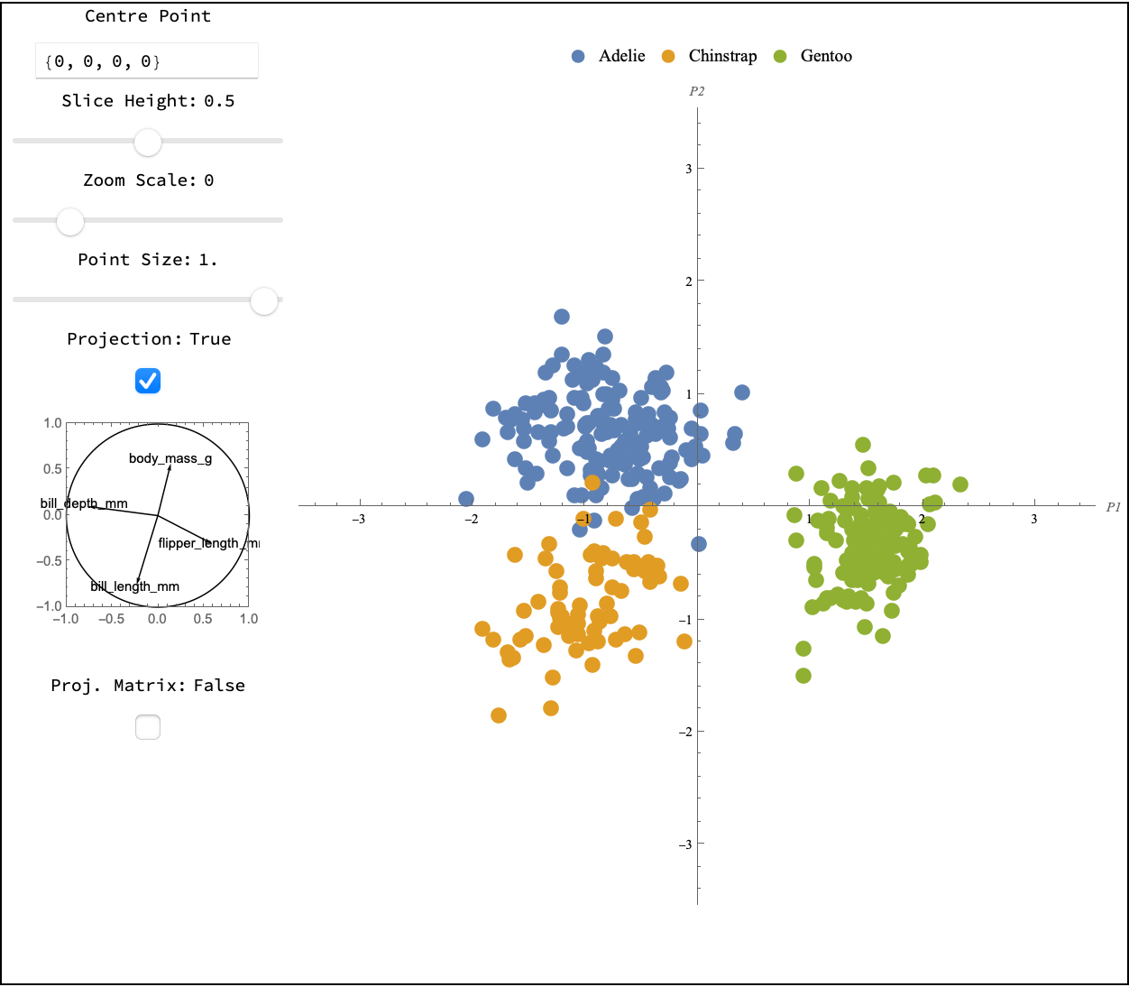
Figure 5: Projection of the data based on $A_{2}$. Compared to projecting onto $A_{1}$ we see that the green observations (Gentoo) are more separated from the other two species.

Finally, to determine which model describes the boundaries better, compare them with the $A_{2}$ projection of the data (Figure 5). Gentoo is more separated from the other two in this projection, and one can imagine that the trees in the forest has greedily grasped any one of many places to make a split to separate the group. It might be argued though the that RF boundary is cut too close to the Chinstrap species, and might lead to some unnecessary misclassification with new data. The LDA boundary is better placed for all species.

This example can be reproduced with the code in penguins_slicing_through_center.nb and a run through is shown in the first part of the video at https://vimeo.com/747590472.

4.4 Shifting the slice center

We have seen that starting from $A_{1}$ using the manual controls to change the contribution of the second variable we could find a clear separation boundary indicating the relation between this variable (bill depth) and the Gentoo penguin species. Instead of rotating to a different projection, we might also change the view by moving the slice along one axis in the 4D space. Here we will continue our exploration of the dependence on bd and move the slice defined by $A_{1}$ to either large positive or negative values ($c^{\pm}_{bd}=\pm 1.5$ after centering and scaling). Thus we define $\mathbf{c}^{\pm}=(0,c^{\pm}_{bd},0,0)$. Here we will also look at slices of the observed data points, using a thicker slice ($h=1.5$) to capture enough points in a given view.

We start by a comparison of the two models and the data distribution shifting to $\mathbf{c}^{+}$, thus the slice is localized towards high values of bill depth in Figure 6. We can see that all three slices (the two models and the data) contain almost no points from the third class (green, Gentoo), and that the decision boundary between the two models is very similar.

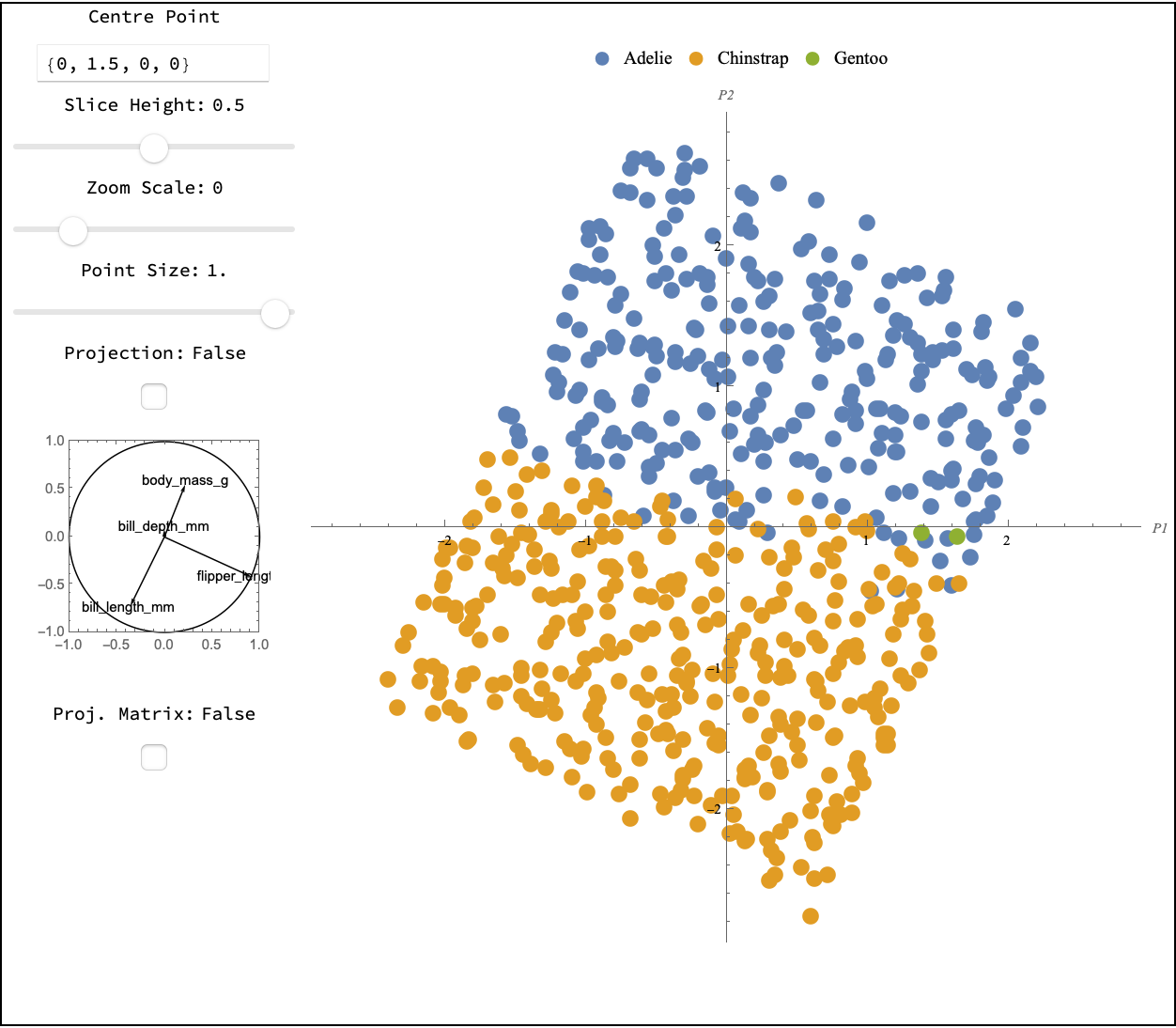
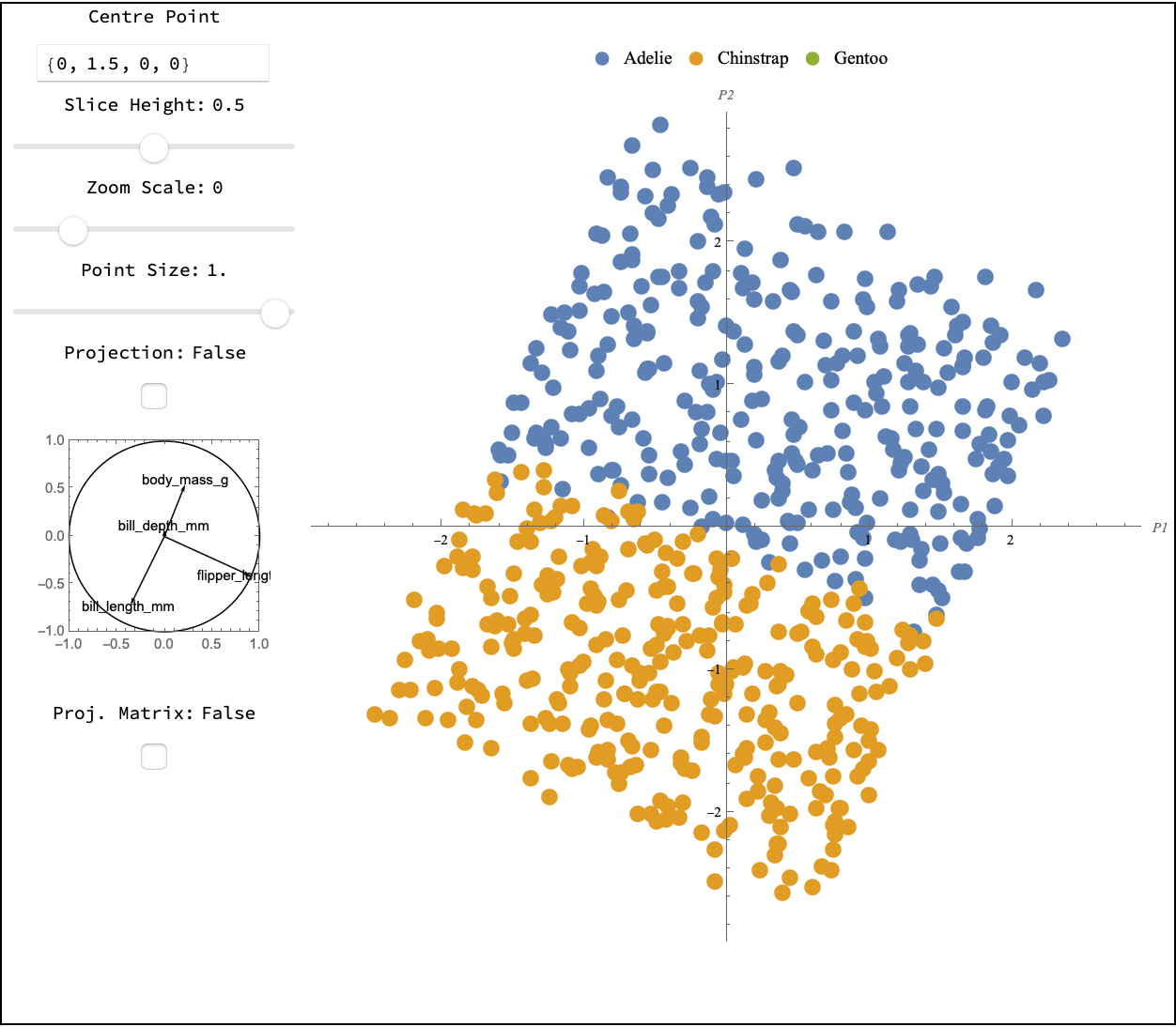
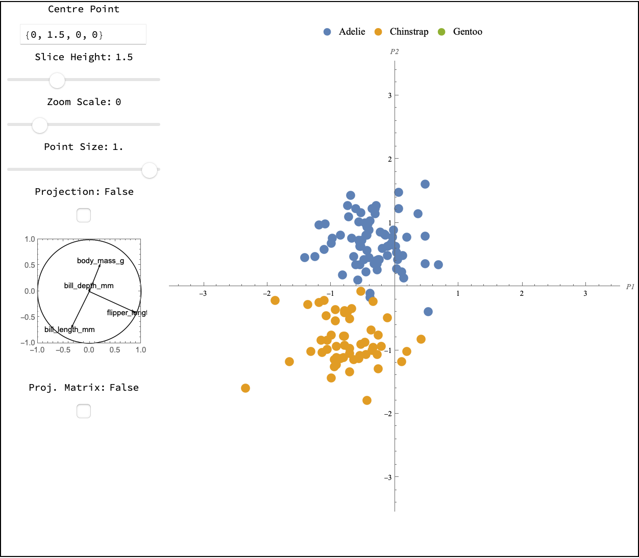
Figure 6: Shifting the slice center in the positive direction of bill depth produces regions that have no Gentoo (green). The two models have similar boundaries except that the RF is more of a step function.

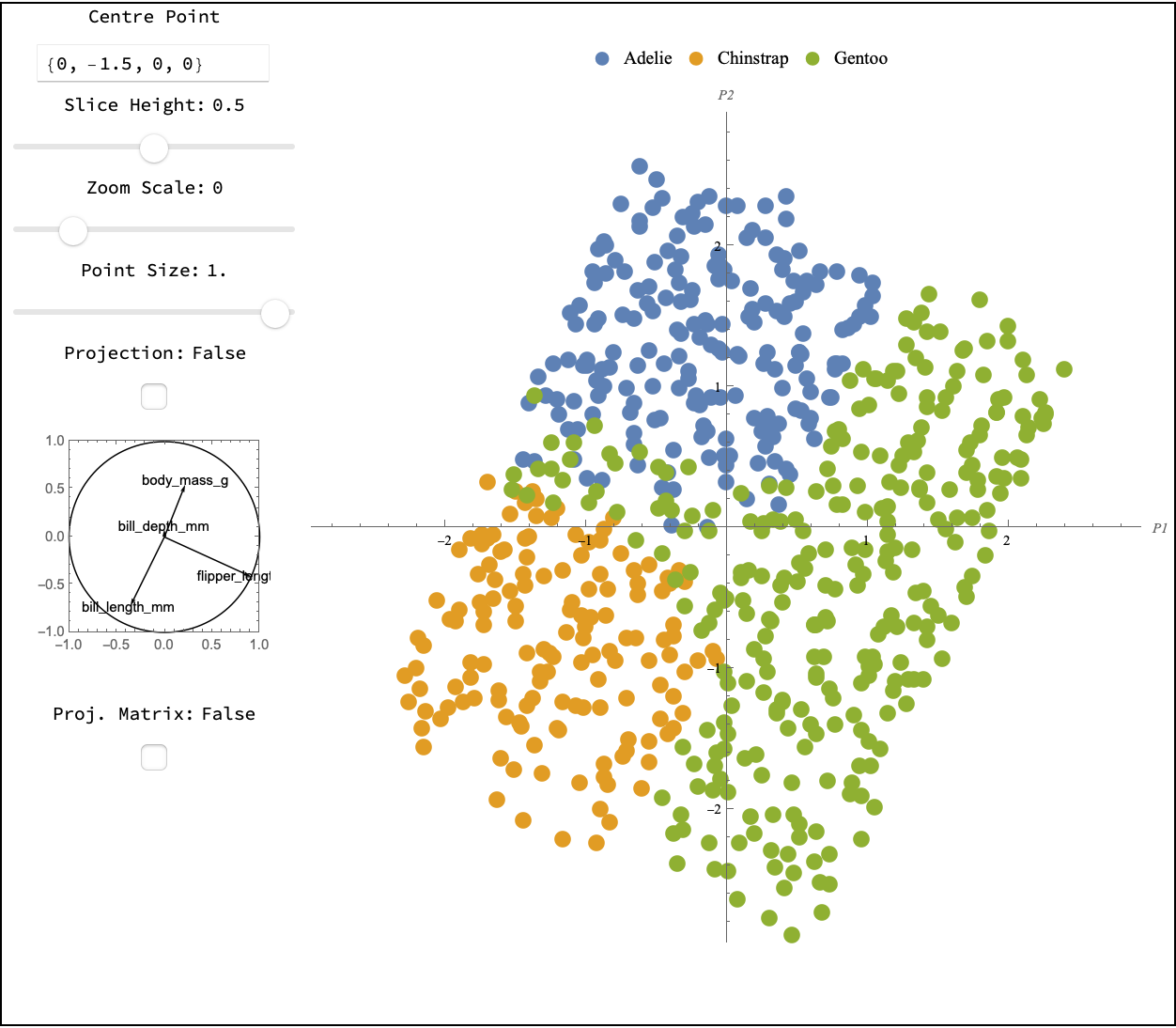
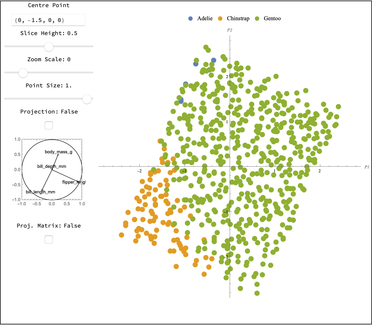
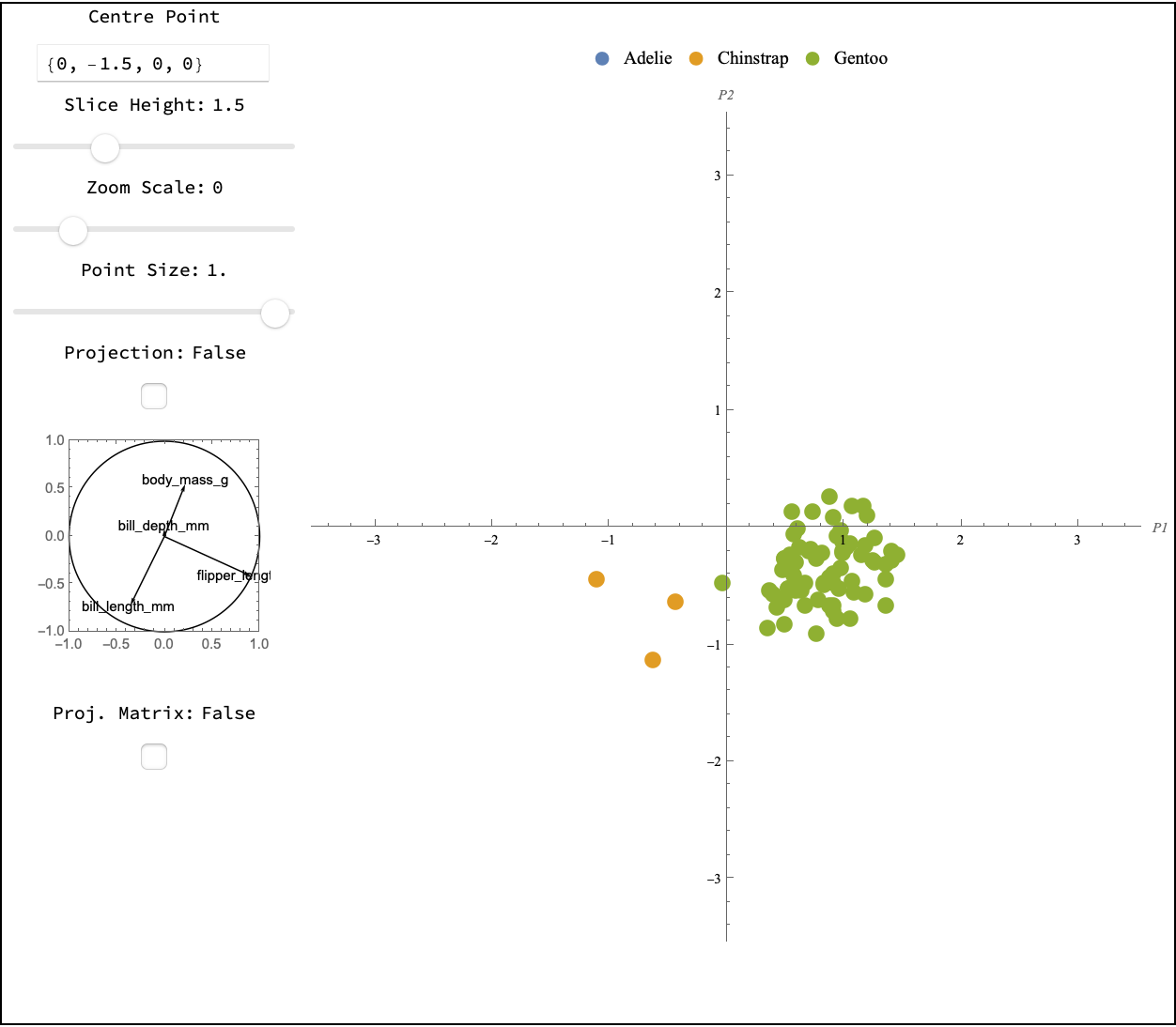
Figure 7: Shifting the slice center in the negative direction of bill depth produces regions that are mostly Gentoo (green). The two models have very different boundaries: the nonlinear potential of RF can be seen here where still some subspaces would predict to be Adelie and Chinstrap.

A more interesting comparison is found for $\mathbf{c}^{-}$, thus the slice localized towards low values of bill depth, shown in Figure 7. The RF model (left) predicts all three species within this slice, with an interesting boundary for the third class (green, Gentoo). On the other hand the LDA model (middle) predominantly predicts the third class within the slice, this appears to be enforced through the linear structure of the model. Looking finally at the thick slice through the data we see that there are primarily observations from this class within the slice we can conclude that the two models have filled in the “empty” space (where we do not have any training observations) in very different ways and according to what we might expect given the model structure.

Finally it is interesting to compare the slice views to the projection of the models seen in Fig. 3 to better understand how the boundaries change along the bd direction and where the differences in the projections come from.

This example can be reproduced with the code in penguins_shifting_slice_center.nb and a run through is shown in the second part of the video at https://vimeo.com/747590472.

5 Discussion

This short note has described new technology for manually interacting with tours. The manual control of projection coefficients is most useful for assessing variable importance to perceived structure, but can be generally used for steering a viewer through high-dimensional space. Changing the center of a slice manually enables exploring the space orthogonal to a projection, specifically in the direction of a single variable. This is a new tool, and as shown in the example, when used with the slice tour can be very useful for understanding boundaries of classifiers. This is also likely a useful method for examining low-dimensional non-linear manifolds, and also functions of multiple parameters.

Mathematica provided a useful sandbox to experiment with the ideas presented in this paper. Most of the data, though, is first constructed using R, especially the classification boundaries. If new technology for interactive graphics becomes available in R it would be useful to create a tighter coupling of models and visualization to allow exploring and comparing fits.

Supplementary material

The source material and animated gifs for this paper are available at https://github.com/uschiLaa/mmtour.

The supplementary materials include:

• The Mathematica source code defining the new functions in mmtour.wl.

• Three Mathematica notebooks with the code used in the application (corresponding to the three subsections).

• Appendix with additional details about manual controls, and Mathematica functions.

• Animations illustrating the manual tour and slicing, matching the static figures in the paper. These are also available at https://vimeo.com/747585410 and https://vimeo.com/747590472.

Appendix A Refinements to enforce exact position

The problem with the new simple method (Algorithm 1) is that the precise values for $V_{m}$ cannot be specified because the orthonormalisation will change them.

A.1 Adjustment method 1

A small modification to algorithm 1 will maintain the components of $V_{m}$ precisely (Figure 8). It is as follows:

1. Provide $A$, and $m$.

2. Change values in row $m$, giving $A^{*}$.

3. Store row $m$ separately, and zero the values of row $m$ in $A^{*}$, giving $A^{*0}$.

4. Orthonormalise $A^{*0}$, using Gram-Schmidt.

5. Replace row $m$ with the original values, giving $A^{**}$.

6. For $d=2$, adjust the values of ${\boldmath a}^{**}_{.2}$ using

$$a^{**}_{j2}+\frac{a_{m1}a_{m2}}{p-1},j=1,...,p,j\neq m.$$

which ensures that

$$\sum_{j=1,j\neq m}^{p}a^{**}_{j1}a^{**}_{j2}+a_{m1}a_{m2}=0.$$

If $d>2$ the process would be sequentially repeated in the same manner that Gram-Schmidt is applied sequentially to orthormalise the columns of a matrix. If $d=1$ no orthonormalisation is needed, and the projection vector would simply need to be normalized after each adjustment.

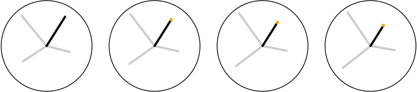
Figure 8: Manual controls with algorithm 2. The precise location of the axis is maintained.

A.2 Adjustment method 2

For $d=2$ projections, the projection matrix is the sub-matrix $A$, of $O$ (an orthonormal basis for the p-dimensional space), formed by its first two columns as illustrated in Eq. (A1) . Whereas orthonormality of the basis for the p-dimensional space is given by $e_{i}\cdot e_{j}=\delta_{ij},{i,j,=1,\cdots,p}$, orthonormality of the projection matrix is expressed as $\sum_{k=1}^{p}a_{ki}a_{kj}=\delta_{ij},~{}{i,j=1,2},~{}{k=1,\cdots,p}$. Movement of the cursor takes the two components ${a_{m1},a_{m2}}$ into a selected new value ${a^{*}_{m1},a^{*}_{m2}}$. Although the motion is constrained by $a^{*2}_{m1}+a^{*2}_{m2}\leq 1$, this is not sufficient to guarantee orthonormality of the new projection matrix. One possible algorithm to achieve this is

1. Cursor movement takes ${a_{m1},a_{m2}}\to{a^{*}_{m1},a^{*}_{m2}}$, called $V_{m}$ above.

2. The freedom to change the components $a_{m3}\cdots a_{mp}$ (the columns of $O$ not corresponding to the projection matrix $A$) is used to select a new orthonormal basis as follows:

   1. For row $m$ one chooses $a^{*}_{m3}=\sqrt{1-a^{*2}_{m1}-a^{*2}_{m1}},~{}a^{*}_{m,k>3}=0$

   2. For other rows, $a_{i\neq m,j\geq 3}$ random selections in the range $(-1,1)$ are made.

   3. The Gram-Schmidt algorithm is then used to obtain an orthonormal basis taking $e_{m}$ as the first vector (which is already normalized), and then proceeding as usual $e_{1}\to e_{1}-(e_{1}\cdot e_{m})e_{m}$, $e_{1}\to e_{1}/(e_{1}\cdot e_{1})$, etc, resulting in $A^{**}$.

3. this results in the orthonormal basis $O^{*}$ and a new projection matrix with $A^{**}_{m1}=a^{*}_{m1},~{}A^{**}_{m2}=a^{*}_{m2}$.

The random completion of $O$ outside the projection matrix provides an exploration of dimensions orthogonal to the projection plane. However, it renders projections in a way that is not continuous and may be distracting. This can be alleviated by replacing the random completion with a rule restricting the size of the jumps, for example in step (b) the values $a_{i\neq m,j\geq 3}$ can be left unchanged before orthogonalisation.

We could also take a similar approach without completing the basis, through rotation within the $d$-dimensional hyperplane defined by the new projection. In that case we would again start from $A^{*}$ as above, and then rotate the basis such that the first direction is aligned with the selected variable $m$. Applying Gram-Schmid within that basis definition will not alter the direction for the first vector, thus the direction of $m$ remains fixed to what was selected with the cursor. By adjusting the normalization procedure we can also ensure that the lenght remains as selcted manually by the user.

Appendix B Slice center guide

The slice center, $c$, from Equation 1 in the main paper, is a point in the $p$-dimensional space. By default, it is placed in the center of the data (Figure 9 A). Moving this along a variable axis moves the slice outwards from the center of the data (Figure 9 B, C). The visual display of the center position is a form of star plot as suggested useful in Hurley, O’Connell, and Domijan (2022), where the position of the point is marked by a polygon on radial axes indicating its position relative to the variable minimum to maximum values.

Figure 9: Visual guide for the slice center. Variable axes are displayed in polar coordinates, where the center corresponds to minimum value and outer end corresponds to maximum value. The position of the center corresponds to the dark polygon. If the center is at the center of the data, this will be displayed as a regular polygon (A), and plots B, C show it’s position when moving the center along one axis.

Appendix C Software details

Here we describe the functions implemented in the Mathematica package mmtour.wl. The main function and its arguments are given below:

SliceDynamic[data, projmat, height, heightRange, legendQ(=1), flagQ(=1), colorFunc(=ColorData[97])]

• data: A data matrix, potentially with grouping that has a label (string) and a flag (numerical) in the last two columns.

• projmat: The initial projection matrix. It is possible to start with a random projection with the input “random” (including the quotes) in this entry field.

• height: The initial height of the slice.

• heightRange: The range of slice heights to be explored.

• legendQ: A flag signaling whether the data matrix includes a column with group labels (1) or not (0).

• flagQ: A flag signaling whether the data matrix includes a numerical flag for the groups.

• colorFunc: specifies the color mapping for the different groups.

The first four arguments are required. As possible starting values we suggest using a random input projection, and selecting slice height parameters using the estimate given in Section 2.4.2 of the paper.

The function renders a manual tour with controls that allow the user to navigate through different projections. For a given projection, a slider permits the user to change the slice width within its range and a separate box switches the view to a projection. The user can also change the center point of slices; the size of the points rendered and the scale of the plot through sliders. An additional box displays the coordinates of the projection matrix explicitly.

This function can be used for ungrouped data by setting legendQ and flagQ to 0. To remove a group from the visual display, the user can choose specific colors for the entry colorFunc. For example, {Red,White,Green} would display groups 1 (red) and 3 (green) while making 2 invisible.

The package includes the additional functions not used in the example application: ProjectionPlot, Projected2DSliderPlot, and VisualiseSliceDyanmic.

ProjectionPlot is very similar to SliceDynamic, except it only displays projections. Using it instead of SliceDynamic simplifies the display and is more efficient. The interface is slightly different, the data file should not contain labels for groups, if these are desired they are passed through the optional argument legendNames as {“group 1”, “group 2”,…}, for example. The function and its arguments are given below:

ProjectionPlot[data, projmat, legendNames(={}), colorFunc(=ColorData[97])]

• data: A data matrix with one or more groups labeled by a flag (numerical, last column).

• projmat: The initial projection matrix. It is possible to start with a random projection with the input “random” (including the quotes) in this entry field.

• legendNames: an optional list of labels for the groups.

• colorFunc: specifies the color mapping for the different groups.

ProjectedLocatorPlot displays the interactive controls slightly differently. Several locator panes are displayed above the display of the projected data and each one corresponds to a row in the projection matrix. The updating behavior of the projection is the same as in ProjectionPlot. The function and its arguments are given below:

ProjectedLocatorPlot[data, projmat, legendNames(={}), colorFunc(=ColorData[97])]

• data: A data matrix with one or more groups labeled by a flag (numerical, last column).

• projmat: The initial projection matrix. It is possible to start with a random projection with the input “random” (including the quotes) in this entry field.

• legendNames: an optional list of labels for the groups.

• colorFunc: specifies the color mapping for the different groups.

Finally VisualiseSliceDynamic allows to discern which points exist inside the slice and outside it. This function differs from SliceDynamic in that it looks at only one data set but displays both the points inside and outside the slice. The display panel allows the user to specify the size of both sets of points (inside and outside) along with the slice height, center point and zoom level. The function and its arguments are given below:

VisualiseSliceDynamic[data, projmat, height, heightRange]

• data: A data matrix containing only one group. In this case the data matrix should not contain column labels.

• projmat: The initial projection matrix. It is possible to start with a random projection with the input “random” (including the quotes) in this entry field.

• height: The initial height of the slice.

• heightRange: The range of slice heights to be explored.

The points inside the slice are shown in black whereas those outside the slice are shown in light blue, with labels indicating this.

References

- ASA Statistical Graphics Section (2022) ASA Statistical Graphics Section. 2022. “Video Library.” https://community.amstat.org/jointscsg-section/media/videos.
- Asimov (1985) Asimov, D. 1985. “The Grand Tour: A Tool for Viewing Multidimensional Data.” SIAM Journal of Scientific and Statistical Computing 6 (1): 128–143.
- Cook and Buja (1997) Cook, Dianne, and Andreas Buja. 1997. “Manual Controls for High-Dimensional Data Projections.” Journal of Computational and Graphical Statistics 6 (4): 464–480. http://www.jstor.org/stable/1390747.
- Emerson et al. (2013) Emerson, John W., Walton A. Green, Barret Schloerke, Jason Crowley, Dianne Cook, Heike Hofmann, and Hadley Wickham. 2013. “The Generalized Pairs Plot.” Journal of Computational and Graphical Statistics 22 (1): 79–91. Accessed 2022-07-14. http://www.jstor.org/stable/43304816.
- Fisherkeller, Friedman, and Tukey (1974) Fisherkeller, M.A., J.H. Friedman, and J.W. Tukey. 1974. “PRIM-9, an interactive multidimensional data display and analysis system.” In The Collected Works of John W. Tukey: Graphics 1965-1985, Volume V, edited by William S. Cleveland, 340–346.
- Horst, Hill, and Gorman (2020) Horst, Allison Marie, Alison Presmanes Hill, and Kristen B Gorman. 2020. palmerpenguins: Palmer Archipelago (Antarctica) penguin data. R package version 0.1.0, https://allisonhorst.github.io/palmerpenguins/.
- Hurley, O’Connell, and Domijan (2022) Hurley, Catherine B., Mark O’Connell, and Katarina Domijan. 2022. “Interactive Slice Visualization for Exploring Machine Learning Models.” Journal of Computational and Graphical Statistics 31 (1): 1–13. https://doi.org/10.1080/10618600.2021.1983439.
- Laa et al. (2022) Laa, Ursula, Dianne Cook, Andreas Buja, and German Valencia. 2022. “Hole or Grain? A Section Pursuit Index for Finding Hidden Structure in Multiple Dimensions.” Journal of Computational and Graphical Statistics 0 (0): 1–14. https://doi.org/10.1080/10618600.2022.2035230.
- Laa, Cook, and Valencia (2020) Laa, Ursula, Dianne Cook, and German Valencia. 2020. “A Slice Tour for Finding Hollowness in High-Dimensional Data.” Journal of Computational and Graphical Statistics 29 (3): 681–687. https://doi.org/10.1080/10618600.2020.1777140.
- Lee et al. (2021) Lee, Stuart, Dianne Cook, Natalia da Silva, Ursula Laa, Earo Wang, Nick Spyrison, and H. Sherry Zhang. 2021. “Advanced Review: The State-of-the-Art on Tours for Dynamic Visualization of High-dimensional Data.” arXiv:2104.08016 [cs, stat] http://arxiv.org/abs/2104.08016.
- Spyrison and Cook (2020) Spyrison, Nicholas, and Dianne Cook. 2020. “spinifex: an R Package for Creating a Manual Tour of Low-dimensional Projections of Multivariate Data.” The R Journal 12 (1): 243. https://journal.r-project.org/archive/2020/RJ-2020-027/index.html.
- Wickham (2016) Wickham, Hadley. 2016. ggplot2: Elegant Graphics for Data Analysis. Springer-Verlag New York. https://ggplot2.tidyverse.org.
- Wickham (2022) Wickham, Hadley. 2022. classifly: Explore Classification Models in High Dimensions. R package version 0.4.1, https://CRAN.R-project.org/package=classifly.
- Wickham, Cook, and Hofmann (2015) Wickham, Hadley, Dianne Cook, and Heike Hofmann. 2015. “Visualizing statistical models: Removing the blindfold.” Statistical Analysis and Data Mining: The ASA Data Science Journal 8 (4): 203–225. https://onlinelibrary.wiley.com/doi/abs/10.1002/sam.11271.
- Wickham et al. (2011) Wickham, Hadley, Dianne Cook, Heike Hofmann, and Andreas Buja. 2011. “tourr: An R Package for Exploring Multivariate Data with Projections.” Journal of Statistical Software 40 (2): 1–18. http://www.jstatsoft.org/v40/i02/.
- Wolfram Research, Inc. (2022) Wolfram Research, Inc. 2022. Mathematica, Version 13.1. Champaign, IL. https://www.wolfram.com/mathematica.
- Xie (2015) Xie, Yihui. 2015. Dynamic Documents with R and knitr. 2nd ed. Boca Raton, Florida: Chapman and Hall/CRC. https://yihui.name/knitr/.
- Xie, Allaire, and Grolemund (2018) Xie, Yihui, Joseph J. Allaire, and Garrett Grolemund. 2018. R Markdown: The Definitive Guide. Chapman and Hall/CRC. https://bookdown.org/yihui/rmarkdown.